Journal of Macroeconomics 31 (2009) 509–522

Contents lists available at ScienceDirect

Journal of Macroeconomics

journal homepage: www.elsevier .com/locate / jmacro

The investment tax credit and irreversible investment

Sumru Altug a,*, Fanny S. Demers b, Michel Demers b

a Koç University and Centre for Economic Policy Research, Rumelifeneri Yolu, Sariyer 34450, Istanbul, Turkeyb Carleton University, 1125 Colonel By Drive, Ottawa, Ontario, Canada K1S 5B6

a r t i c l e i n f o a b s t r a c t

Article history:Received 1 February 2008Accepted 5 January 2009Available online 14 January 2009

JEL classification:E22E6H2H3

Keywords:Irreversible investmentInvestment tax creditTax policyChanges in persistenceIncreases in risk

0164-0704/$ - see front matter � 2009 Elsevier Incdoi:10.1016/j.jmacro.2009.01.001

* Corresponding author. Tel.: +90 2123381673; faE-mail address: saltug@ku.edu.tr (S. Altug).

1 Among these we may note Lucas (1976), Abel (19to which we refer below. For a current review of tax

We examine the impact of random changes in investment tax credit (ITC) policy on theirreversible investment decisions of a monopolistically competitive firm facing demanduncertainty. We examine the impact of increases in risk and changes in persistence inthe ITC policy on investment behavior. Our results indicate that a temporary ITC (lowerpolicy persistence) generally increases the variability of investment both in the shortand the long-run. It lowers investment in the short-run and raises it in the long-run. Thus,perhaps surprisingly, a temporary ITC does not always lead to higher investment butalways leads to more volatile investment. Policy-makers may thus face a long-run trade-off between the level and the volatility of investment. We also find that increases in riskdefined in terms of mean-preserving spreads may lead to lower investment.

� 2009 Elsevier Inc. All rights reserved.

1. Introduction

Governments frequently modify tax laws, be it with the intent of stabilizing the economy through countercyclical actions,of stimulating the level of investment and long-run growth, of changing the composition of investment or of reducing itsvolatility. In a recent paper, Romer and Romer (2007b) argue that tax changes have a much stronger impact on real GDP thanfound in previous studies. They show that a 1% increase in taxes (as a percentage of GDP) reduces real GDP by 2–3% in USpostwar data, and they trace the source of this effect to the strong (negative) impact of the tax change on investment. Thus,investment seems to be the component of GDP that is the most sensitive to tax changes. The investment tax credit (ITC) hasbeen a popular fiscal tool to influence the level of investment for reasons of macro-stabilization or to stimulate specific sec-tors. While there has not been any ITC at the federal level since 1986, more recently there has been some support for thenotion of reintroducing an ITC as a cost-effective way of stimulating investment. In addition, there are a very large numberof sector-specific ITC measures that are provided at the state level.

Few papers have investigated the impact of tax policy uncertainty on investment decisions.1 Yet, this topic is of theoret-ical, empirical and policy importance for developed, semi-industrialized and transition economies alike. For example, since tax

. All rights reserved.

x: +90 2123381659.

82), Bizer and Judd (1989), Aizenman and Marion (1993), and more recently, Hassett and Metcalf (1999),policy, see Hassett and Hubbard (2002).

510 S. Altug et al. / Journal of Macroeconomics 31 (2009) 509–522

policy often responds to economic conditions, firms may assign a positive probability that an investment tax credit (ITC) couldbe put in place should aggregate investment decline or should long-run growth issues become a public concern. Alternativelyfirms may anticipate a reduction or elimination of the ITC should there be an overheating of the economy.2 Such considerationswould affect both the timing and the amount of investment undertaken by firms. Uncertainty about the ITC could be expectedto have an even more pronounced impact when investment is irreversible.

In this paper, we examine the impact of changes in the ITC in a framework where investment decisions are irreversible,and where firms must decide on whether to invest, and if so, how much. Hence, uncertainty may affect both the timing ofinvestment (the extensive margin) and the quantity of investment (the intensive margin). In our framework, a change in thecurrent value of the ITC affects investment directly through the current cost of investing and also by its informational con-tent as it signals higher or lower values of future ITCs. Due to irreversibility, the anticipation of future tax changes affectsinvestment by altering the expected marginal value of capital and the endogenous risk premium or option value of waiting.

We focus on the impact of changes in the persistence and volatility of the ITC. Hassett and Metcalf (1999) observe that theITC seems to be better characterized by a stationary Poisson process in US post-war data. They assume in their study that theITC follows a 2-state Poisson process, and analyse the impact of a mean-preserving spread (MPS) in this setting. We too assumethat the ITC follows a Poisson process. However, US postwar data show that ITC changes may be more accurately characterizedas a three-state process. Romer and Romer (2007a) provide a very extensive documentation of all tax changes in post-war USdata.3 For the period between 1946 and 1996, we note from their study that an ITC was first introduced in 1962 as a permanentmeasure, and was generally in effect from 1962 until the tax reform of 1986. During this period, the ITC went through severalchanges some of which were announced as being temporary and others permanent. It was temporarily suspended in 1966 forapproximately one year, reinstated in 1967 (with a higher ceiling), repealed in 1969, reinstated (and temporarily increased) in1971, reduced permanently in 1982 and finally repealed in the 1986 tax reform. There was no ITC between 1946 and 1962 andbetween 1986 and 1996. Thus, focusing on the period between 1946 and 1996, we may characterize the ITC as an on–off Poissonprocess with three states: a low state (ITC off), a high state (ITC on and high) and a medium state (ITC on but lower).4 Hence, weconsider a three-state (high/medium/low) Poisson process5 to investigate the impact of both greater persistence and volatility.

It may alternatively be argued that when policy changes, the probability of another change occurring very soon thereaftershould be low since it takes at least four quarters to implement a new fiscal policy. By contrast, the probability of a changeshould be much higher if the policy has been in place for a substantial amount of time. In order to capture this effect, weconsider an alternative non-Poisson third order Markovian process for the ITC where the ITC state is duration-dependent:the longer a given ITC state has been in place, the lower the probability of remaining in that state. The impact of persistenceand volatility is investigated in this model as well.

We first consider the impact of changes in the persistence of the ITC. In a context of certainty, the impact of higher taxincentives depend on whether they are temporary or permanent. A temporary ITC is typically expected to have a greater im-pact than a permanent one because it induces an intertemporal reallocation of investment. Under uncertainty, we examine theimpact of the permanence of an ITC by investigating how changes in the persistence of tax incentives affect investment. Weshow that more temporary ITCs (lower policy persistence) lead to greater variability of investment. In addition, using numer-ical simulations, we also show that more temporary ITC’s do not always lead to higher investment, but always lead to greatervariability. When setting the ITC, policy-makers may face a trade-off between higher versus more stable investment.

We next consider the impact of increases in risk in the ITC. In their analysis of mean-preserving spreads (MPS) in the ITCwhen firms must optimally choose the time to undertake an irreversible investment project, Hassett and Metcalf (1999) findthat an increase in tax risk actually reduces the time to invest. Hence, they conclude that greater randomness in the ITC in-creases investment. We show that Hasset and Metcalf’s findings can be attributed in our framework to the impact of a ‘‘cur-rent cost” effect of a change in tax policy as firms seek to take advantage of higher than average tax incentives. We also showthat in the context of the three-state Poisson model, when the firm faces uncertainty not only with respect to the timing ofthe change in the ITC (as in the two-state Poisson model), but also with respect to the direction and magnitude of the changein the ITC, greater randomness in the ITC in the sense of a mean-preserving spread lowers investment.

The remainder of this paper is organized as follows: Sections 2 and 3 present the theoretical framework and the simula-tion results, respectively, while Section 4 concludes.

2. The theoretical framework

Consider the problem of a monopolistically competitive risk neutral firm that faces uncertainty in its environment arisingfrom shocks to demand and from randomness in tax policy.

2 Numerous tax provisions affect corporate investment, three of the most noteworthy being the statutory corporate profits tax rate, depreciation allowanceschedules, and the investment tax credit (ITC). All three affect the tax wedge, or the percentage of the purchase price of investment that the firm must pay. Anexamination of US tax policy shows that the tax wedge has been volatile at times partly as a result of changes in the ITC.

3 See also Altug et al. (2004) for an analysis of the ‘‘tax wedge” affecting real investment decisions.4 Specifically, the ITC changes can be categorized as:1946—1961|fflfflfflfflfflfflfflfflffl{zfflfflfflfflfflfflfflfflffl}

no ITC

1962—1965|fflfflfflfflfflfflfflfflffl{zfflfflfflfflfflfflfflfflffl}med ITC

1966—1967|fflfflfflfflfflfflfflfflffl{zfflfflfflfflfflfflfflfflffl}no ITC

1967—1968|fflfflfflfflfflfflfflfflffl{zfflfflfflfflfflfflfflfflffl}high ITC

1969—1970|fflfflfflfflfflfflfflfflffl{zfflfflfflfflfflfflfflfflffl}no ITC

1971—1981|fflfflfflfflfflfflfflfflffl{zfflfflfflfflfflfflfflfflffl}high ITC

1982—1985|fflfflfflfflfflfflfflfflffl{zfflfflfflfflfflfflfflfflffl}med ITC

1986—1996|fflfflfflfflfflfflfflfflffl{zfflfflfflfflfflfflfflfflffl}no ITC

.

5 More accurately, we assume the ITC follows a mixed Poisson process. A change in the ITC occurs in accordance with a Poisson jump process as in Hassettand Metcalf (1999), but conditional on a change occurring, the value of the ITC is itself random and may take on one of two values. In HM, conditional on achange occurring, the value of the ITC is known to the firm.

S. Altug et al. / Journal of Macroeconomics 31 (2009) 509–522 511

Assume that the firm’s production function is given by FðAt ;Kt ; LtÞ, where At denotes a random technology shock, Kt de-notes the stock of capital, and Lt a vector of variable inputs. Also assume that the firm faces a constant elasticity demandfunction. The choice of variable inputs L�ðKt ;at ;At ;wtÞ involves a static maximization problem under certainty. Define theshort-run profit function PðKt ;at ;At ;wtÞ as a function of the current capital stock Kt , the shock to demand at , the technologyshock At , and the vector of variable input prices wt . P is continuous in Kt , at , At , wt , increasing in Kt , at , and At , decreasing inwt , and strictly concave in Kt . Henceforth we suppress At and wt as arguments of P.

Let st denote the corporate tax rate at time t, Dx;t�x depreciation allowances per dollar invested for tax purposes for capitalequipment of age x on the basis of the tax law effective at time t � x, and T the life of the equipment. Let it denote the nominalrate of interest, r the real rate of interest and pe

t the expected rate of inflation where it ¼ r þ pet . Define zt as the present value

of tax deductions on new investment, where zt ¼PT

n¼1stþnDn;tð1þ itÞ�n. Letting pkt denote the purchase price of investment

goods, and ct denote the stochastic ITC, we can define pIt � ð1� ct � ztÞpk

t as the tax-adjusted price of investment. Note thatthe term ð1� ct � ztÞ is the ‘‘stochastic tax wedge” or after-tax percentage of pk

t that the firm pays for investment goods. Wecan now express the firm’s after-tax cash flow as Rt ¼ ð1� stÞPðKt;at ;At ;wtÞ � pI

tIt where It is the firm’s gross investmentmeasured in physical units. The corporate tax rate affects the firm’s net cash flow and the tax allowed deductions for depre-ciation, while the ITC alters the relative price of new and used investment goods.

The focus of our analysis is an examination of random changes in ITC policy in the presence of demand uncertainty andirreversibility. We consider two types of ITC policy: exogenous and endogenous. When policy is exogenous, ctþ1 is a seriallycorrelated random variable which depends only on the past value ct . However, when policy is endogenous the distribution ofctþ1 will also depend on at , thus capturing the countercyclical nature of policy. Considering both cases let Gcðctþ1jct ;atÞ bethe distribution function of ctþ1. We also assume that at and ct are mutually independent and that at is a serially correlatedrandom variable, with distribution Gaðatþ1jatÞ. Both Gcðctþ1jct ;atÞ and Gaðatþ1jatÞ are known to the firm.6 The time paths of allprices and productivity are known to the firm. Denote by Et the expectation operator using the conditional distributions of atþ1

and ctþ1. Using dynamic programming, we can express the firm’s optimality problem recursively:

6 Thapolicy.

7 Ut �

VðKt; ct ;atÞ ¼maxItð1� stÞPðKt;atÞ � pI

tIt þ bEtVðKtþ1; ctþ1;atþ1Þ� �

subject to the irreversibility constraint It P 0 and the law of motion of capital, Ktþ1 ¼ ð1� dÞKt þ It , where Kt is given and d,0 < d < 1 is the deterministic depreciation rate, Also, b ¼ ð1þ rÞ�1, 0 < b < 1. (For brevity, we supress At and wt as state vari-ables.) Let VK denote the partial derivative of V with respect to K. The first-order necessary and sufficient conditions for theoptimization problem at time t are

�pIt þ bEtVKðKtþ1; ctþ1;atþ1Þ 6 0; with equality for I�t > 0: ð1Þ

Define at by

pIt ¼ b

Z 1

0

Z 1

0VKðð1� dÞKt ; ctþ1;atþ1ÞdGaðatþ1jatÞdGcðctþ1jct ; atÞ ð2Þ

For any Kt , ct , pkt ;G

aðatþ1jatÞ, and Gcðctþ1jct ;atÞ there is a critical or threshold value, atð�Þ such that the expected marginalvalue of capital conditional on at is equal to pI

t with zero investment. For at 6 at there is zero investment while for at >

at , It > 0. Using the envelope theorem, the shadow price of capital is given by

VKðKtþ1; ctþ1;atþ1Þ ¼ ð1� stþ1ÞPKðKtþ1;atþ1Þ þ ð1� dÞmin pItþ1;bEtþ1VKðð1� dÞKtþ1; ctþ2;atþ2Þ

� �: ð3Þ

Assume I�t > 0. After substituting for VK and b, (1) can be re-arranged as

ct þUt ¼ 1� stþ1ð ÞEtPK Ktþ1;atþ1;At;wtð Þ ð4Þ

where PK is the partial derivative of P with respect to Ktþ1. The right-hand side of (4) is the marginal benefit of investing anadditional unit. The left-hand side is the total cost of investing which is the sum of the Jorgensonian cost of capital,ct ¼ pI

tðr þ dÞ � ð1� dÞðEtpItþ1 � pI

tÞ, and of Ut , an endogenous and time-varying marginal risk premium. With irreversibleinvestment and uncertainty about future demand and the after-tax costs of investing, firms are cautious. They prefer to in-vest less than they would if they could sell excess capital, for fear of being stuck with too much capital.7 The optimality con-dition (1) can be presented alternatively as

pIt þ bCL

K Ktþ1; pItþ1

� �¼ Nt þ!t � bEt 1� stþ1ð ÞPK Ktþ1;atþ1;htþ1ð Þ þ b 1� dð ÞEtþ1VKðð1� dÞKtþ1; ctþ2;atþ2Þ

� �ð5Þ

where CLK is the marginal call option, Nt is the expected marginal value of capital if the firm neither invests nor disinvests

from t þ 1 onward, and simply allows its capital stock to depreciate, while !t represents the increase in the expected mar-ginal value of capital due to future growth options available to the firm. The marginal call option, CL

K is an additional cost thatmust be taken into account when investment is irreversible since by investing one additional unit at t, the firm loses theoption to wait and invest that unit at t þ 1. This additional cost discourages investment. It plays a role analogous to the exog-enous marginal cost of adjustment but is endogenous and time-varying. See Demers et al. (2003).

t is, there is no subjective uncertainty with respect to tax policy. We analyse this issue in a companion paper where we allow for learning about taxSee Altug et al. (2007b). In Altug et al. (1999) we analyze the case of subjective uncertainty with respect to the unknown costs of investing.ð1� dÞfEt pk

tþ1 � Et min½pktþ1; bEtþ1VK ðð1� dÞKtþ1Þ�g, and captures the forward-looking nature of the firm’s problem. (See Demers, 1991).

512 S. Altug et al. / Journal of Macroeconomics 31 (2009) 509–522

The first-order conditions permit us to obtain oIt=oct , i.e., the impact of a change in the current ITC on current investment.When ct is serially independent and policy is exogenous, a higher current ITC has a current cost reducing effect, and stimulatesinvestment.8 When there is serial dependence, however, a change in ct will also have an additional information effect since itaffects both the distribution function Gcðctþ1jct;atÞ and the future marginal value of capital VK . That is, assuming I�t > 0, andintegrating the numerator by parts we obtain

8 Asslead to

9 Mo10 It c

price ofseriallyTherefo

11 Tha12 As

whereconditi

oIt

oct¼ pk

t

�bR

VKK dGaðatþ1jatÞdGcðctþ1jct ;atÞ�

bR

VKcGcctðctþ1jct ;atÞdctþ1

�bR

VKK dGaðatþ1jatÞdGcðctþ1jct ;atÞð6Þ

the first term being the positive cost reducing effect and the second, the information effect. The sign of the information effectdepends on the sign of VKc and of Gc

ct� oG=oct , the shift in the distribution of ctþ1 caused by an increase in ct . When ctþ1 is

positively serially correlated (p.s.c.), the higher the current value of ct , the higher is the probability of observing a high valueof the ITC next period, and Gc

ct6 0.9 Furthermore, in this case VKc < 010 so that the information effect is negative. Intuitively,

the expectation of ‘‘good times” ahead, reduces the urgency to invest today. This effect dampens the impact of the positive costreducing effect, and as a result the total impact of an increase in ct on current investment is ambiguous. However, our simu-lation results indicate that the cost effect dominates in most cases, so that oIt=oct > 0, and an increase in the current ITC in-creases current investment under positive serial correlation. In the case of negative serial correlation (n.c.), Gc

ctP 0.11

Assuming (in accordance with our simulation results) that VKc < 0, the information effect is positive so that both the costand the information effects are conducive to stimulating current investment, and oIt=oct > 0. In this case, an increase in the cur-rent ITC will increase current investment.

To sum up: this analysis indicates that an increase in the ITC today does not automatically lead to an increase in investment.The impact depends crucially on the characteristics of the distribution of the ITC and on how expectations of the future are affectedby this change.

Consider now a change in government where the new administration is favourable to increasing the ITC without speci-fying its exact level. Such a situation can be characterized as an exogenous FSD shift in the distribution of the future ITC, suchthat all the moments of the new distribution are now larger. In other words, the probability of a higher future ITC increaseswith a shift in the distribution and the firm now expects a higher ITC on average, but is also more uncertain of its true value.For a given observed value of ct , ctþ1 is said to be ‘‘stochastically larger” under the new distribution cGc than under Gc, orequivalently, cGc dominates Gc by FSD. The impact of such a shift depends on the sign of VKc. Since VKc < 0 when c is p.s.c.or i.i.d., the firm delays and reduces current investment under cGc12 since it expects more generous incentives in the future.The same is true for the case of negative serial correlation if VKc < 0.

When the ITC is endogenous, under countercyclical policy a high state of demand at t will lead to a lower ITC at t + 1, thatis, Gc

atP 0. Thus, if the state of demand is higher at t, say a0t > at , Gcðctþ1jct ;a0tÞ will be stochastically smaller than

Gcðctþ1jct ;atÞ. Thus, if VKc < 0 then Ið�;Gcðctþ1jct ;a0tÞÞ > Ið�;Gcðctþ1jct ;atÞÞ. Current investment will rise in anticipation of fu-ture cuts in the ITC.

2.1. Changes in persistence

In a context of certainty, the impact of a larger ITC depends on whether it is temporary or permanent. A temporary ITC istypically expected to have a greater impact because it induces an intertemporal reallocation of investment. Under uncer-tainty, since the ITC is random, the permanence of an ITC is examined by investigating changes in the persistence of theITC process. Greater policy persistence in the ITC makes it more likely that current tax incentives will be maintained inthe future. In this section we show that changes in the persistence of the ITC may affect not only the magnitude but alsothe volatility of investment.

Consider two possible distributions for ct such that the distribution ðGc2Þ is more persistent than the original distributionðGc1Þ and where ct 2 ½cL; cH�. We use the FSD-ranking of these distributions and the sign of oIt=oct , which we discussed earlierin Section 2, to establish the impact of greater persistence on the variability of investment. Note that conditional on ct ¼ cL

uming an interior solution at time t, oIt=oct ¼ pkt �b

RVKK dGaðatþ1jatÞdGcðctþ1Þ

� ��1> 0. In the case of a corner solution at time t, an increase in ct will

a lower incidence of a binding constraint.re specifically, Gcðctþ1jc0t ;atÞ dominates Gcðctþ1jct ;atÞ in the sense of first-order stochastic dominance (FSD) for all c0t P ct , for any given at and for all t.an be shown that VKc is unambiguously negative when c is positively serially correlated or when it is i.i.d. With positive correlation, a lower after-taxinvestment at t þ 1 raises capital accumulation at t þ 1 and a higher ITC at t þ 1 signals an even higher one in the future. However, when c is negativelycorrelated, a higher ITC signals a lower one in the future, so that VKc is theoretically indeterminate. Our simulation results indicate that VKc < 0.

re, our discussion below will focus on the case VKc < 0.t is, Gcðctþ1jct ;atÞ dominates Gcðctþ1jc0t ;atÞ by FSD for all c0t P ct and for all at .can be easily shown,Z

VK ðKtþ1; ctþ1;atþ1ÞðdcGc ðctþ1jct ;atÞ � dGcðctþ1jct ;atÞÞdGaðatþ1jatÞ ¼Z

VKcðKtþ1; ctþ1;atþ1ÞðGcðctþ1jct ;atÞ � cGc ðctþ1jct ;atÞÞdctþ1 < 0 when VKc < 0:

the equality follows from using integration by parts. Hence, denoting the optimal investment under Gc and cGc by I�Gc and I�bGc, from the first-order

on (1), I�bG < I�G when VKc < 0.

S. Altug et al. / Journal of Macroeconomics 31 (2009) 509–522 513

the distribution function exhibiting greater persistence ðGc2Þ attaches greater probability to lower realizations of ctþ1 thanGc1. In this case, Gc1ðctþ1jcL;atÞ dominates Gc2ðctþ1jcL;atÞ by FSD for any at , and in view of our discussion in Section 2,IðKt ; cL;Gc1Þ < IðKt ; cL;Gc2Þ.13 However, conditional on ct ¼ cH , Gc2 assigns greater probability to high realizations of ctþ1 thanGc1 and hence now Gc2ðctþ1jcH;atÞ dominates Gc1ðctþ1jcH;atÞ by FSD for any at . In this case, IðKt ; cH;Gc1Þ > IðKt ; cH;Gc2Þ. Sincethe policy function IðKt ; ct ;G

c1Þ is continuous in ct , there exists some c such that IðKt ; c;Gc1Þ ¼ IðKt ; c;Gc2Þ, andIðKt ; c;Gc1Þ < IðKt; c;Gc2Þ for cL

6 c < c, while IðKt; c;Gc1Þ > IðKt ; c;Gc2Þ for c < c 6 cH .Turning to the inaction zone, proceeding analogously we can show: (1) conditional on cL, at is lower with Gc2 and the

size of the inaction zone falls: aðKt ; cL;Gc2Þ 6 aðKt ; cL;Gc1Þ; (2) conditional on cH , at is higher with Gc2 and the size of theinaction zone increases: aðKt ; cH;Gc2ÞP aðKt ; cH;Gc1Þ. When the ITC is low there are fewer states of demand for which itis optimal to refrain from investing when the ITC becomes more persistent. Conversely, when the ITC is high and morepersistent there are more states of demand for which it is propitious not to invest. By continuity, there exists some csuch that aðKt ; c;Gc1Þ ¼ aðKt ; c;Gc2Þ, and aðKt ; c;Gc1Þ > aðKt ; c;Gc2Þ for cL

6 c < c, and aðKt ; c;Gc1Þ < aðKt ; c;Gc2Þ forc < c 6 cH .

We summarize our results as follows:

Proposition 1

(i) When oIt=oct > 014 greater persistence in the ITC induces lower variability of investment, that is,IðKt ; cH;Gc1ÞP IðKt; cH ;Gc2ÞP IðKt ; cL;Gc2ÞP IðKt ; cL;Gc1Þ and aðKt ; cH;Gc1Þ 6 aðKt ; cH;Gc2Þ 6 aðKt ; cL;Gc2Þ 6 aðKt ; cL;Gc1Þ.

(ii) When oIt=oct < 015 greater persistence in the ITC induces greater variability of investment, that is,IðKt ; cL;Gc2ÞP IðKt ; cL;Gc1ÞP IðKt ; cH;Gc1ÞP IðKt ; cH;Gc2Þ and aðKt ; cL;Gc2Þ 6 aðKt ; cL;Gc1Þ 6 aðKt ; cH;Gc1Þ 6 aðKt ; cH;Gc2Þ.

As we noted above, our simulations reveal oIt=oct > 0. Therefore, by Proposition 1 more permanent incentives lower thevariability of investment. Conversely, resorting to temporary incentives increases fluctuations in investment. However, sincewe cannot conclude a priori that a temporary ITC will have a greater impact on the average level of investment nor on theaverage size of the inaction zone we will ascertain this by using simulations in Section 3.16

2.2. Increases in risk and persistence: A Poisson model for the ITC

Hassett and Metcalf (1999) note that in US post-war data the ITC seems to be characterized by a stationary Poisson pro-cess, randomly switching from a high to a low state. The 2-state Poisson model assumes that the investment tax credit cantake on two possible values (or ‘‘states”), cH > cL. The number of changes in the ITC expected in a given time period is equalto ki for i ¼ L;H. Alternatively, we can say that the expected persistence of a given state i is 1=ki. In addition, the probability ofobserving at least one change in the ITC in the next period is 1� e�ki for i ¼ L;H, and the probability of no change is e�ki

where 1=ki represents the persistence of state i. In this paper we will consider a more general stationary Poisson process suchthat the probability of at least one change in the ITC in the next period is 1� e�ki as in the 2-state case, but conditional on achange occurring, the ITC is random, and may take on one of two possible values different from the current one. This impliesthat overall, the ITC may take on three possible values which we label high, medium and low with cH > cM > cL. Thus, con-ditional on being in the low state there is a positive probability pLM of moving to a middle state, and ð1� pLMÞ probability ofmoving to a high state, should there be a change in the ITC. The transition matrix for this ‘‘3-state Poisson” model can bewritten as

13 Her

where t14 Tha15 Tha16 Thi

technol(2002).

P ¼

e�kL pLMð1� e�kL Þ ð1� pLMÞð1� e�kL Þ

pMLð1� e�kM Þ e�kM ð1� pMLÞð1� e�kM Þ

ð1� pHMÞð1� e�kH Þ pHMð1� e�kH Þ e�kH

2664

3775: ð7Þ

In our simulations, we take p ¼ 0:5 for all cases.To address endogenous policy changes, we allow the persistence of an ITCstate to be a function of at , the state of demand facing the firm, by letting kH

t ¼ �kþ /ðat � �aÞ, kMt ¼ �kþ /ðat � �aÞ and

kLt ¼ �k� /ðat � �aÞ where �k is the exogenous component of persistence common to all three states, �a denotes the average

e we are considering the case of VKc < 0. This result follows from the fact that

bZ

VK ðKtþ1; ctþ1;atþ1ÞdGc1ðctþ1jcLÞdGaðatþ1jatÞ 6 bZ

VK ðKtþ1; ctþ1;atþ1ÞdGc2ðctþ1jcLÞdGaðatþ1jatÞ 6 ð1� cL � ztÞpkt ;

he first inequality follows from FSD dominance of Gc1 over Gc2 with VKc < 0, and the second inequality comes from the first-order condition.t is, when ct is positively correlated and the cost effect dominates, or when ct is negatively correlated and VKc < 0.t is, when ct is positively serially correlated and the information effect dominates, or ct is negatively correlated and VKc > 0.s is in contrast with results obtained under certainty. For example, in a cost of adjustment model under certainty with a decreasing returns to scaleogy and perfect competition Abel (1982) demonstrates that a temporary ITC has a greater impact on current investment. See also Hassett and Hubbard

514 S. Altug et al. / Journal of Macroeconomics 31 (2009) 509–522

state of demand and / denotes the strength of the response to deviations from average demand.17 Note that k becomes time-varying in this framework. Thus, during a boom when at is high relatively to �a, kH

t rises and the persistence of the ITC falls (theITC becomes more temporary). Conversely, during a recession at is low relatively to �a, kH

t falls and the ITC becomes more per-sistent. The same is true for kM . If the economy is in a low ITC state, kL

t falls with an increase in a and rises with a fall in a. That is,the persistence of a low ITC states increases if there is a boom and falls if there is a recession. We note that the exogenous policymodel is a special case of the endogenous policy model. Hence, we analyse persistence and the impact of increases in risk underthe more general endogenous policy model.18 We analyse policy persistence as well as increases in risk in the ITC in thiscontext.

The merits of this approach are two fold. First, as evidenced by Romer and Romer’s (2007a) recent analysis of post-war UStax policy, a three-state model seems to better characterize US post-war experience regarding the ITC relative to a two-statemodel. Secondly, the three-state case permits an analysis of the firm’s behaviour when it is confronted with uncertainty bothwith respect to the timing of the change in the ITC and with respect to the magnitude or direction of the change. Note that inthe two-state Poisson model, the firm is uncertain as to when or whether a change in the ITC will occur. However, condi-tional on being in the high state, the firm knows with certainty that if the ITC changes, it will fall and that it will take theknown value cL. Similarly, conditional on being in the low state, it knows with certainty that the ITC will increase to cH ifthere is a change in the ITC. By contrast, in the three-state case, if a change in the ITC occurs, conditional on being in thehigh state, the firm knows that the ITC will fall, but does not know whether it will take on the value cM or cL. Conditionalon being in the low state, the firm knows that the ITC will rise, but does not know whether it will take on the value cM

or cH . Furthermore, the firm faces even greater uncertainty when it is in the middle state since it does not even knowwhether the ITC will rise or fall should a change occur. In this middle state, it is also possible to change the distributionof the ITC without changing its current value, thus eliminating the ‘‘current cost reducing” effect. This permits us to isolatethe risk effect. As a result, we are able to capture the impact of greater risk alone and we find that a MPS in the ITC reducesinvestment in the long-run as we show in Section 3 below.

2.3. Duration dependence

By portraying changes in policy as Poisson processes, we are in fact assuming that the probability of a change in the ITC isindependent of its duration, that is, of how long it has been in place. It may alternatively be argued that when policy changes,the probability of another change occurring very soon thereafter should be low since it takes at least four quarters to imple-ment a new fiscal policy. By contrast, the probability of a change should be much higher if the policy has been in place for asubstantial amount of time. According to this argument, the probability of changes in policy should be dependent on thelength of stay in a given state. Introducing duration dependence makes the process non-Poisson. In order to maintain therecursive structure of the model, we introduce duration dependence as follows.19 Let d denote the duration of the stay ina particular state to date. Suppose that an ITC remains unchanged on average for three years, so that we let the maximum valueof the duration parameter be 3. This determines the memory of the system. The state vector at t is given by fðst ; dtÞg wherest ¼ L;M;H denotes the ITC state and d ¼ 1;2;3 denotes the duration ‘‘state”. By introducing the duration parameter as an addi-tional state variable, we are in fact reducing a 3rd order Markov process (since the probability depends on the previous threestates) to a first-order process, and we are thus maintaining the recursive structure of the model. This system with 3 ITC statesand a maximum duration parameter of 3 yields a sparse 9 � 9 transition probability matrix. We provide the full matrix in Table5 in the Appendix. The law of motion of the duration parameter is

17 Wedemand

18 In fendoge

19 DurDurlanddepend

20 Alteadvanta

dt ¼ 1 if st–st�1

dt ¼ dt�1 þ 1 if st ¼ st�1 and dt�1 < 3 ð8Þdt ¼ dt�1 if st ¼ st�1 and dt�1 ¼ 3

The transition probabilities are expressed as follows.We express the probability of observing no change in the ITC at time tconditional on being (say) in the low state at time t � 1 and conditional on (say) dt�1 ¼ 1, as probðLt ;2jLt�1;1Þ ¼ e�kLþaL�bL1

where aL is a constant and bL is a parameter indicating the sensitivity to duration.20 According to this specification, the prob-ability of remaining in the same state diminishes as the duration in that state increases. The specification must satisfy therestrictions that each entry in the transition matrix must be positive and less than one (since it represents a probability),and the sum over the states must be equal to one for each time period. Note that this specification also nests the case whichis duration independent by letting a ¼ 0 and b ¼ 0. For example, with �k ¼ 0:35, a ¼ 0:5 and b ¼ 0:3 we get:

also performed simulations with an alternative specification where kLt ¼ �k� /at ; k

M ¼ �kþ /at , kHt ¼ �kþ /at and responds directly to the level of

. The results were very similar to the deviations case.act, we performed numerical simulations for both the endogenous and exogenous cases, but since the results are very similar, we only report thenous policy results.ation dependence has been introduced in Markov-switching models of GNP growth rates (see for example, Diebold et al. (1994), Filardo (1994) and

and McCurdy (1994)). In this paper we follow the approach of Durland and McCurdy. See Altug et al. (2007a) for an alternative model of durationence in a regime-switching model of political risk.rnatively, we could have used a different specification for the transition probabilities, namely, e�kLþaL�bL dt�1

1þe�kLþaL�bL dt�1. However, our current specification has the

ge of nesting the Poisson model.

Table 1Parameter values.

� g b d s w pk A q rm

�3.607 0.346 0.947 0.13 0.4817 8 1.18 6 0.75 0.1323

S. Altug et al. / Journal of Macroeconomics 31 (2009) 509–522 515

e�0:35þ0:5�0:3ð1Þ ¼ 0:860 71, e�0:35þ0:5�0:3ð2Þ ¼ 0:637 63, e�0:35þ0:5�0:3ð3Þ ¼ 0:472 37 as d ¼ 1;2 and 3 respectively. Thus, as d in-creases, the probability of remaining in the same state decreases. Below, we investigate the impact of persistence and of in-creases in risk with this duration-dependent model as well.

3. Numerical results

The simulations assume a constant returns to scale Cobb–Douglas production function: Yt ¼ AtKgt L1�g

t where 0 < g < 1.The inverse market demand function is given by pt ¼ ðatÞ�

1eðYtÞ

1e where e < �1 is the price elasticity of demand and at is

the stochastic state of demand.Table 1 shows the baseline parameter values used in the simulations. Our simulations apply to US manufacturing. We

identify the elasticity of demand from markup estimates for US manufacturing industries. The constant values for w, pk,and A, are obtained using manufacturing data on real wages, the real price of capital, and an estimate of the Solow residual.Our model abstracts from general equilibrium considerations, which would affect the discount factor for the firm’s futurecash flows. We consider a constant discount factor, namely, b ¼ 0:947, which implies an annual real interest rate ofr ¼ 5:6%. We assume that lnðatÞ follows a stationary ARð1Þ process with a mean of zero, autoregressive parameterq ¼ 0:75, and unconditional standard deviation ra ¼ 0:2. (The implied conditional standard deviation is rm ¼ 0:1323.) Weapproximate the continuous ARð1Þ process for the demand shock with a discrete Markov chain following the approach de-scribed by Tauchen (1986). There are 100 points in the capital stock grid and 100 points in the grid for the demand shock.

We focus on tax incentives for shorter-lived assets such as producers’ durable equipment of various categories. Thus, weset the depreciation rate d equal to 0.13 as the average depreciation rate for equipment assets considered by Jorgenson andYun (1991), Table 3.19, p.79. Likewise, ct and the present value of depreciation allowances, zt , are measured as the averagerates of the ITC and of depreciation allowances for equipment assets. We consider alternative processes for the ITC and thestochastic tax wedge over the period 1946–1996. For the case of a discrete ITC, we set z equal to its sample average over theentire period, that is, z ¼ 0:40. Finally, we set the corporate tax rate, s, equal to its average value for the sample period 1946–1996, that is, s ¼ 0:4817. Thus, we abstract from variations in the corporate tax rate st .

3.1. Changes in persistence

Table 2 shows the parameterizations for the 3-state Poisson model used in our analysis for endogenous policy. Looking atthe first column for the specifications, we consider one distribution where cL ¼ cM ¼ cH (distribution I, the certainty case),and two distributions where cL < cM < cH and the values of the ITC differ between the three states. In particular, in distri-bution II, cL ¼ 0:05, cM ¼ 0:10 and cH ¼ 0:15 while in distribution III, cL ¼ 0:0, cM ¼ 0:10 and cH ¼ 0:20. Note that the uncon-ditional mean of c is the same in all of these distributions since the unconditional probability of each state is 0.334. We alsoconsider three sets of values for the parameter �k, going from �k ¼ 1:0968 (the ITC lasts on average about one year), to �k ¼ 0:35(the ITC lasts on average 3 years) to �k ¼ 0:2 (the ITC lasts on average 5 years). We have taken the value of / ¼ 0:08.21 Column1 reports the incidence of a binding irreversibility constraint conditional on observing cL cM , or cH respectively (and hence implyPrðIt > 0Þ for each state,) while column 2 reports the amount of investment undertaken by the firm in each state, provided It > 0,that is, provided the irreversibility constraint is not binding and the firm decides to invest. In column 4 we calculate E(I), averageinvestment across ITC states at time t for each distribution. The calculation EðItÞ where EðItÞ ¼ PrðIt > 0ÞEðItjIt > 0Þ takes intoaccount the average incidence of a binding irreversibility constraint (reported in column 3). Column 5 indicates the coefficientof variation (CV) of investment for each distribution and each value of �k. Columns 6 and 7 provide the long-run results. We cal-culate long-run average investment over several periods for each distribution assuming the firm starts with a medium level ofinitial capital stock kmed

0 , and also measure the coefficient of variation in each case.Clearly, when cL ¼ cM ¼ cH ¼ 0:10 (the certainty case) policy is the most persistent (in fact, constant) and the average le-

vel of investment at time t is 0.395 with a CV of 0.91 regardless of the value of �k. Also the long-run average level of invest-ment is 0.178 with a CV of 0.77 (as indicated in column 7).

We first note that a policy where the ITC is permanent, that is, one where the ITC is maintained at 10% at all times, gen-erally leads to lower investment than one where there are fluctuations in the ITC.22 However, this comes at the cost of greater

21 The exogenous and endogenous policy results are quite similar. We have also performed simulations with / ¼ 0:15 and 0.30, and obtained the samequalitative (and even quantitative) results. For economy of space, we do not report them here. They are available upon request.

22 One exception is the case of k ¼ 1:0986, where (both for endogenous and exogenous policy) average short-run investment actually falls relative to thecertainty case for distribution II, while its variability greatly increases.

Table 2Impact of persistence: 3-state Poisson model, endogenous policy, ð/ ¼ 0:08Þ.

Specification Short-run Long-run ðkmed0 Þ

For cL; cM ; cH Over all c Over all c

(1) (2) (3) (4) (5) (6) (7)For all �k EðIt=0Þ EðItÞ EðIt ¼ 0Þ EðItÞ CV EðItÞ CV

I. cL ¼ cM ¼ cH ¼ 0:1034,34,34 0.395,0.395,0.395 34.3 0.395 0.91 0.178 0.77(6,6,6) (0.12,0.12,0.12) (6) (0.12) (0.1) (0.03) (0.2)

II. cL ¼ 0:05; cM ¼ 0:10; cH ¼ 0:15�k ¼ 1:0986 71,44,18 0.044,0.248,0.793 44 0.361 1.31 0.214 1.64

(6,6,5) (0.02,0.08,0.16) (6) (0.09) (0.1) (0.05) (0.3)

�k ¼ 0:35 56,37,18 0.125,0.350,0.800 37 0.423 1.11 0.205 1.40(6,6,5) (0.05,0.10,0.17) (5) (0.10) (0.1) (0.06) (0.4)

�k ¼ 0:2 51,35,19 0.169,0.374,0.760 35 0.434 1.05 0.195 1.19(6,6,5) (0.06,0.11,0.17) (6) (0.11) (0.11) (0.06) (0.4)

III. cL ¼ 0:00; cM ¼ 0:10; cH ¼ 0:20�k ¼ 1:0986 92,54,8 0.003,0.140,1.20 52 0.446 1.47 0.284 1.85

(28,6,5) (0.003,0.05,0.22) (4) (0.09) (0.09) (0.07) (0.45)

�k ¼ 0:35 73,41,7 0.037,0.278,1.27 40 0.530 1.28 0.249 1.76(6,6,4) (0.02,0.08,0.22) (5) (0.11) (0.09) (0.10) (0.6)

�k ¼ 0:2 65,38,7 0.072,0.334,1.24 37 0.547 1.19 0.231 1.47(6,6,5) (0.03,0.09,0.23) (5) (0.12) (0.1) (0.11) (0.6)

516 S. Altug et al. / Journal of Macroeconomics 31 (2009) 509–522

variability. We can see that the CV substantially increases as we move from a permanent ITC to one that varies. This is true bothfor the short-run (column 5) and for the long-run (column 7). Given a variable ITC, however, Table 2 also reveals that persistenceof policy matters. Looking at the level of investment in the short-run (column 4), and at its variability in the short-run (column5) we observe that for a given distribution of c, the greater is persistence, (i.e, the lower is �k), the larger is average investment inthe short-run and the lower its variability. In the long-run, as capital adjustments take place, the greater is persistence the smal-ler is average investment, and the lower its variability (column 6 and 7). These short-run and long-run results confirm our earliertheoretical analysis for oIt=oct > 0 in Section 2.1 that greater persistence leads to lower variability. We note that while the var-iability of investment falls with greater persistence both in the short-run and the long-run (in accordance with our theoreticalprediction) the level of investment risesin the short-run but falls in the long-run as persistence increases. This result holds forboth distributions II and III.23 Hence, the usual prediction of higher investment for more temporary ITC applies in the long-runbut not in the short-run. Thus, considering the response of investment averaged over all values of the ITC, we find that less per-sistent ITC processes stimulate investment in the long-run at the same time as they increase its variability. Consequently, ourresults indicate that policy-makers face a trade-off in the long-run between a higher level of investment versus more stableinvestment.

We also examine how variations in �k affect the size of the inaction zone both by looking at the incidence of the bindingconstraint in Table 2 and also by looking at the impact of persistence on the boundary value of the inaction zone, a. First,column 1 indicates the incidence of a binding irreversibility constraint (out of 100) conditional on cL; cM and cH , respectively.We note that the lower the persistence of the ITC state, the greater the incidence of a binding constraint conditional on cL.The same conclusion may be observed in the case of cM , though the impact of persistence is less pronounced.When we con-dition on cH the numerical results become more sensitive to the actual value of cH than to the degree of persistence. Thus, theinaction zone is greatly reduced as the value of cH increases from 0.15 to 0.20. For a given value of cH the inaction zone re-mains the same regardless of the degree of persistence. Column 3 provides the incidence of a binding irreversibility con-straint averaged over all three c values. Here we observe that the inaction zone clearly increases as the ITC state becomesless persistent.

We also analyse the impact of persistence on the boundary value of the inaction zone, a. We report these results in graph-ical form. As can be seen from panels (a, b, and c) of Fig. 1, conditional on cL, the value of a (for a given capital stock) riseswith lower persistence. Thus the inaction zone is larger with lower persistence.This is also true in the case of cM , though theimpact of persistence is smaller. In the case of cH , as panel (c) of Fig. 1 shows, greater persistence leads to a higher a but theimpact of persistence is much less pronounced than in the case of lower levels of the ITC. That is, in the case of cH the inactionzones for the three values of persistence almost coincide. It is clear from Fig. 1 that our analysis of a confirms our theoretical

23 We have also investigated the response of investment to a change in the persistence of one state while keeping the persistence of the other one constant.We find that, in general, the above results are confirmed.

0 20 40 60 80 1000

50

100

capital

alph

ahat

gamma−L, Dist. II

0 20 40 60 80 1000

50

100

capital

alph

ahat

gamma−M, Dist. II

0 20 40 60 80 1000

50

100

capital

alph

ahat

gamma−H, Dist. II

lambda=1.0986lambda=0.35lambda=0.2

Fig. 1. The impact of persistence on the boundary value of the inaction zone (Distribution II).

S. Altug et al. / Journal of Macroeconomics 31 (2009) 509–522 517

predictions about a in Section 2. Fig. 1 also confirms the above remarks about the inaction zone based on column 1 of Table 2.The inaction zone becomes much smaller as the value of the ITC increases from cL to cH . Analysing the impact of persistenceon a for distribution III leads to a similar result: the inaction zone further increases for cL and to a lesser extent for cM ,

0 20 40 60 80 1000

50

100

capital

alph

ahat

gamma−L, Dist. III

0 20 40 60 80 1000

50

100

capital

alph

ahat

gamma−M, Dist. III

0 20 40 60 80 1000

50

100

capital

alph

ahat

gamma−H, Dist. III

lambda=1.0986lambda=0.35lambda=0.2

Fig. 2. The impact of persistence on the boundary value of the inaction zone (Distribution III).

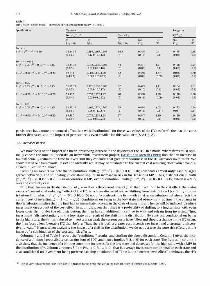
Table 3The 3-state Poisson model – Increases in risk, endogenous policy ð/ ¼ 0:08Þ.

Specification Short-run Long-run

For cL; cM ; cH Over all c kmed0 ; cM

0

(1) (2) (3) (4) (5) (6) (7)EðIt ¼ 0Þ EðItÞ EðIt ¼ 0Þ EðItÞ CV EðItÞ CV

For all kI. cL ¼ cM ¼ cH ¼ 0:10 34,34,34 0.395,0.395,0.395 34.3 0.395 0.91 0.178 0.68

(6,6,6) (0.12,0.12,0.12) (6) (0.12) (0.1) (0.03) (0.2)

For k ¼ 1:0986II. cL ¼ 0:05; cM ¼ 0:10; cH ¼ 0:15 71,44,18 0.044,0.248,0.793 44 0.361 1.31 0.128 0.57

(6,6,5) (0.02,0.08,0.16) (6) (0.09) (0.1) (0.02) (0.2)

III. cL ¼ 0:00; cM ¼ 0:10; cH ¼ 0:20 92,54,8 0.003,0.140,1.20 52 0.446 1.47 0.085 0.70(28,6,5) (0.003,0.05,0.22) (4) (0.09) (0.09) (0.02) (0.2)

For k ¼ 0:35II. cL ¼ 0:05; cM ¼ 0:10; cH ¼ 0:15 56,37,18 0.125,0.350,0.800 37 0.423 1.11 0.164 0.61

(6,6,5) (0.05,0.10,0.17) (5) (0.10) (0.1) (0.03) (0.2)

III. cL ¼ 0:00; cM ¼ 0:10; cH ¼ 0:20 73,41,7 0.037,0.278,1.27 40 0.530 1.28 0.138 0.56(6,6,4) (0.02,0.08,0.22) (5) (0.11) (0.09) (0.02) (0.2)

For k ¼ 0:2II. cL ¼ 0:05; cM ¼ 0:10; cH ¼ 0:15 51,35,19 0.169,0.374,0.760 35 0.434 1.05 0.173 0.64

(6,6,5) (0.06,0.11,0.17) (6) (0.11) (0.11) 0.03 0.2

III. cL ¼ 0:00; cM ¼ 0:10; cH ¼ 0:20 65,38,7 0.072,0.334,1.24 37 0.547 1.19 0.159 0.60(6,6,5) (0.03,0.09,0.23) (5) (0.12) (0.1) (0.03) (0.2)

518 S. Altug et al. / Journal of Macroeconomics 31 (2009) 509–522

persistence has a more pronounced effect than with distribution II for these two values of the ITC; as for cH , the inaction zonefurther decreases, and the impact of persistence is even smaller for this value of c (See Fig. 2).

3.2. Increases in risk

We now focus on the impact of a mean-preserving increase in the riskiness of the ITC. In a model where firms must opti-mally choose the time to undertake an irreversible investment project, Hassett and Metcalf (1999) find that an increase intax risk actually reduces the time to invest and they conclude that greater randomness in the ITC increases investment. Weshow that in our framework, Hasset and Metcalf’s result may be attributed to the current cost reducing effect which we dis-cussed in Section 2.1 above.

Focusing on Table 3, we note that distribution I with ðcL; cM ; cHÞ ¼ ð0:10;0:10;0:10Þ constitutes a ‘‘certainty” case. A largerspread between cL and cH holding cM constant implies an increase in risk in the sense of a MPS. Thus, distributions III withðcL; cM ; cHÞ ¼ ð0:0;0:15;0:20Þ is an unconditional MPS over distribution II with ðcL; cM ; cHÞ ¼ ð0:05;0:10;0:15Þ which is a MPSover the certainty case.

Note that changes in the distribution of ct also affects the current level of ct , so that in addition to the risk effect, there alsoexists a ‘‘current cost reducing ” effect of the ITC which we discussed above. Shifting from distribution I (certainty) to dis-tribution II for which ðcL; cM; cHÞ ¼ ð0:5;0:10;0:15Þ not only confronts the firm with a riskier distribution but also affects thecurrent cost of investing pI

t ¼ ð1� zt � ctÞpKt . Conditional on being in the low state and observing cL at time t, the change in

the distribution implies that the firm has an immediate increase in the costs of investing and hence will be induced to reduceinvestment on account of the cost effect. In addition, given that there is a probability of shifting to a higher state with evenlower costs than under the old distribution, the firm has an additional incentive to wait and refrain from investing. Thus,investment falls substantially in the low state as a result of the shift in the distribution. By contrast, conditional on beingin the high state, the firm is induced to invest a great deal: the current costs have fallen and should a change in the ITC occur,the firm faces a less favorable ITC than before. Thus, there is both a greater cost incentive to invest and a stronger disincen-tive to wait.24 Hence, when analysing the impact of a shift in the distribution, we do not observe the pure risk effect, but theimpact of a combination of the cost and risk effects.

Columns 1 and 2 of Table 3 report the ‘‘conditional” results, and confirm the above discussion. Column 1 gives the inci-dence of a binding irreversibility constraint (out of 100) and hence implies PrðIt > 0Þ for each state. The figures in column 1also show that the incidence of a binding constraint increases for the low state and decreases for the high state with a MPS inthe distribution of c. Column 2 reports EðItÞ ¼ PrðIt > 0ÞEðItjIt > 0Þ, that is, average investment conditional on each state andalso conditional on investment being positive. Looking at column 2 of Table 3, the ‘‘current level effect” dominates the risk

24 This is very similar to the ‘‘use it or lose it” situation facing firms that are in the high ITC state in Hassett and Metcalf (1999).

0 20 40 60 80 1000

50

100

capital

alph

ahat

lambda=1.0986

Dist. IIDist. III

0 20 40 60 80 1000

50

100

capital

alph

ahat

lambda=0.35

0 20 40 60 80 1000

50

100

capital

alph

ahat

lambda=0.2

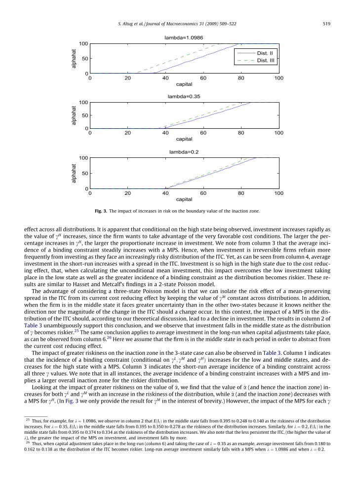
Fig. 3. The impact of increases in risk on the boundary value of the inaction zone.

S. Altug et al. / Journal of Macroeconomics 31 (2009) 509–522 519

effect across all distributions. It is apparent that conditional on the high state being observed, investment increases rapidly asthe value of cH increases, since the firm wants to take advantage of the very favorable cost conditions. The larger the per-centage increases in cH , the larger the proportionate increase in investment. We note from column 3 that the average inci-dence of a binding constraint steadily increases with a MPS. Hence, when investment is irreversible firms refrain morefrequently from investing as they face an increasingly risky distribution of the ITC. Yet, as can be seen from column 4, averageinvestment in the short-run increases with a spread in the ITC. Investment is so high in the high state due to the cost reduc-ing effect, that, when calculating the unconditional mean investment, this impact overcomes the low investment takingplace in the low state as well as the greater incidence of a binding constraint as the distribution becomes riskier. These re-sults are similar to Hasset and Metcalf’s findings in a 2-state Poisson model.

The advantage of considering a three-state Poisson model is that we can isolate the risk effect of a mean-preservingspread in the ITC from its current cost reducing effect by keeping the value of cM constant across distributions. In addition,when the firm is in the middle state it faces greater uncertainty than in the other two-states because it knows neither thedirection nor the magnitude of the change in the ITC should a change occur. In this context, the impact of a MPS in the dis-tribution of the ITC should, according to our theoretical discussion, lead to a decline in investment. The results in column 2 ofTable 3 unambiguously support this conclusion, and we observe that investment falls in the middle state as the distributionof c becomes riskier.25 The same conclusion applies to average investment in the long-run when capital adjustments take place,as can be observed from column 6.26 Here we assume that the firm is in the middle state in each period in order to abstract fromthe current cost reducing effect.

The impact of greater riskiness on the inaction zone in the 3-state case can also be observed in Table 3. Column 1 indicatesthat the incidence of a binding constraint (conditional on cL; cM and cHÞ increases for the low and middle states, and de-creases for the high state with a MPS. Column 3 indicates the short-run average incidence of a binding constraint acrossall three c values. We note that in all instances, the average incidence of a binding constraint increases with a MPS and im-plies a larger overall inaction zone for the riskier distribution.

Looking at the impact of greater riskiness on the value of a, we find that the value of a (and hence the inaction zone) in-creases for both cL and cM with an increase in the riskiness of the distribution, while a (and the inaction zone) decreases witha MPS for cH . (In Fig. 3 we only provide the result for cM in the interest of brevity.) However, the impact of the MPS for each c

25 Thus, for example, for k ¼ 1:0986, we observe in column 2 that EðItÞ in the middle state falls from 0.395 to 0.248 to 0.140 as the riskiness of the distributionincreases. For k ¼ 0:35, EðItÞ in the middle state falls from 0.395 to 0.350 to 0.278 as the riskiness of the distribution increases. Similarly, for k ¼ 0:2, EðItÞ in themiddle state falls from 0.395 to 0.374 to 0.334 as the riskiness of the distribution increases. We also note that the less persistent the ITC, (the higher the value ofk), the greater the impact of the MPS on investment, and investment falls by more.

26 Thus, when capital adjustment takes place in the long-run (column 6) and taking the case of k ¼ 0:35 as an example, average investment falls from 0.180 to0.162 to 0.138 as the distribution of the ITC becomes riskier. Long-run average investment similarly falls with a MPS when k ¼ 1:0986 and when k ¼ 0:2.

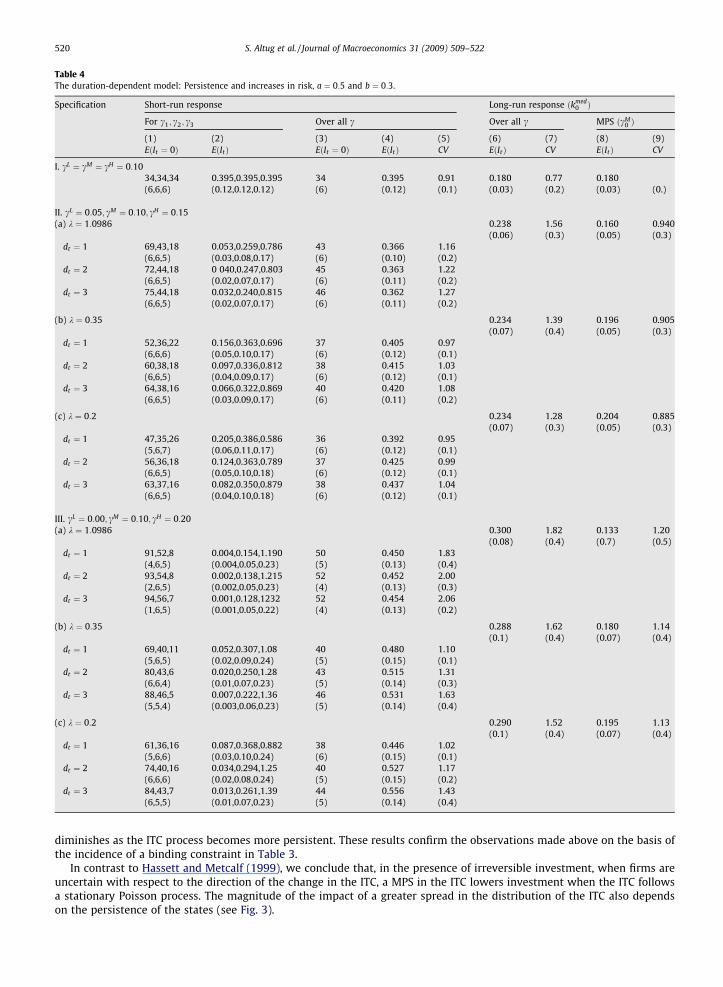
Table 4The duration-dependent model: Persistence and increases in risk, a ¼ 0:5 and b ¼ 0:3.

Specification Short-run response Long-run response ðkmed0 Þ

For c1; c2; c3 Over all c Over all c MPS ðcM0 Þ

(1) (2) (3) (4) (5) (6) (7) (8) (9)EðIt ¼ 0Þ EðItÞ EðIt ¼ 0Þ EðItÞ CV EðItÞ CV EðItÞ CV

I. cL ¼ cM ¼ cH ¼ 0:1034,34,34 0.395,0.395,0.395 34 0.395 0.91 0.180 0.77 0.180(6,6,6) (0.12,0.12,0.12) (6) (0.12) (0.1) (0.03) (0.2) (0.03) (0.)

II. cL ¼ 0:05; cM ¼ 0:10; cH ¼ 0:15(a) k ¼ 1:0986 0.238 1.56 0.160 0.940

(0.06) (0.3) (0.05) (0.3)dt ¼ 1 69,43,18 0.053,0.259,0.786 43 0.366 1.16

(6,6,5) (0.03,0.08,0.17) (6) (0.10) (0.2)dt ¼ 2 72,44,18 0 040,0.247,0.803 45 0.363 1.22

(6,6,5) (0.02,0.07,0.17) (6) (0.11) (0.2)dt ¼ 3 75,44,18 0.032,0.240,0.815 46 0.362 1.27

(6,6,5) (0.02,0.07,0.17) (6) (0.11) (0.2)

(b) k ¼ 0:35 0.234 1.39 0.196 0.905(0.07) (0.4) (0.05) (0.3)

dt ¼ 1 52,36,22 0.156,0.363,0.696 37 0.405 0.97(6,6,6) (0.05,0.10,0.17) (6) (0.12) (0.1)

dt ¼ 2 60,38,18 0.097,0.336,0.812 38 0.415 1.03(6,6,5) (0.04,0.09,0.17) (6) (0.12) (0.1)

dt ¼ 3 64,38,16 0.066,0.322,0.869 40 0.420 1.08(6,6,5) (0.03,0.09,0.17) (6) (0.11) (0.2)

(c) k ¼ 0:2 0.234 1.28 0.204 0.885(0.07) (0.3) (0.05) (0.3)

dt ¼ 1 47,35,26 0.205,0.386,0.586 36 0.392 0.95(5,6,7) (0.06,0.11,0.17) (6) (0.12) (0.1)

dt ¼ 2 56,36,18 0.124,0.363,0.789 37 0.425 0.99(6,6,5) (0.05,0.10,0.18) (6) (0.12) (0.1)

dt ¼ 3 63,37,16 0.082,0.350,0.879 38 0.437 1.04(6,6,5) (0.04,0.10,0.18) (6) (0.12) (0.1)

III. cL ¼ 0:00; cM ¼ 0:10; cH ¼ 0:20(a) k ¼ 1:0986 0.300 1.82 0.133 1.20

(0.08) (0.4) (0.7) (0.5)dt ¼ 1 91,52,8 0.004,0.154,1.190 50 0.450 1.83

(4,6,5) (0.004,0.05,0.23) (5) (0.13) (0.4)dt ¼ 2 93,54,8 0.002,0.138,1.215 52 0.452 2.00

(2,6,5) (0.002,0.05,0.23) (4) (0.13) (0.3)dt ¼ 3 94,56,7 0.001,0.128,1232 52 0.454 2.06

(1,6,5) (0.001,0.05,0.22) (4) (0.13) (0.2)

(b) k ¼ 0:35 0.288 1.62 0.180 1.14(0.1) (0.4) (0.07) (0.4)

dt ¼ 1 69,40,11 0.052,0.307,1.08 40 0.480 1.10(5,6,5) (0.02,0.09,0.24) (5) (0.15) (0.1)

dt ¼ 2 80,43,6 0.020,0.250,1.28 43 0.515 1.31(6,6,4) (0.01,0.07,0.23) (5) (0.14) (0.3)

dt ¼ 3 88,46,5 0.007,0.222,1.36 46 0.531 1.63(5,5,4) (0.003,0.06,0.23) (5) (0.14) (0.4)

(c) k ¼ 0:2 0.290 1.52 0.195 1.13(0.1) (0.4) (0.07) (0.4)

dt ¼ 1 61,36,16 0.087,0.368,0.882 38 0.446 1.02(5,6,6) (0.03,0.10,0.24) (6) (0.15) (0.1)

dt ¼ 2 74,40,16 0.034,0.294,1.25 40 0.527 1.17(6,6,6) (0.02,0.08,0.24) (5) (0.15) (0.2)

dt ¼ 3 84,43,7 0.013,0.261,1.39 44 0.556 1.43(6,5,5) (0.01,0.07,0.23) (5) (0.14) (0.4)

520 S. Altug et al. / Journal of Macroeconomics 31 (2009) 509–522

diminishes as the ITC process becomes more persistent. These results confirm the observations made above on the basis ofthe incidence of a binding constraint in Table 3.

In contrast to Hassett and Metcalf (1999), we conclude that, in the presence of irreversible investment, when firms areuncertain with respect to the direction of the change in the ITC, a MPS in the ITC lowers investment when the ITC followsa stationary Poisson process. The magnitude of the impact of a greater spread in the distribution of the ITC also dependson the persistence of the states (see Fig. 3).

S. Altug et al. / Journal of Macroeconomics 31 (2009) 509–522 521

3.3. The model with duration dependence

In this section we investigate numerically the impact of greater persistence and greater riskiness in the model with dura-tion dependence described in Section 2.3 above. For ease of comparison with our Poisson model, we consider the same valuesof k, namely k ¼ 1:0986;0:35 and 0.2 even though the k’s no longer represent arrival rates. We also let a ¼ 0:5 and b ¼ 0:3.From Table 4 Column 5, reporting the value of the CV, we observe that for each value of k, variability increases as the dura-tion parameter d increases from 1 to 3 since the probability of remaining in the same state (and hence its persistence) falls asd increases. Comparing across k values, the probability of remaining in the same state is highest when k ¼ 0:2 (except for thecertainty case), and we observe that in this case the CV values are also the lowest at each value of d. Thus, for example, in thecase of distribution II, k ¼ 0:2 yields the lowest CV values of 0.95,0.99 and 1.04 for d ¼ 1;2;3, respectively. This result con-firms once more our theoretical prediction that greater persistence leads to lower volatility of investment. Column 3 revealsthat for each k value, the incidence of a binding constraint rises (and the inaction zone increases) as d increases. In otherwords, as the probability of remaining in the same state next period falls, the inaction zone increases. The same resultmay be observed across k values, with the largest inaction zone being observed for k ¼ 1:0986 and the smallest for k ¼ 0:2.

With respect to the impact of increases in risk, Table 4 Column 2 reveals that conditional on cM , for each value of k and foreach level of the parameter d, investment is lower for distribution III relative to distribution II and relative to distribution I(the certainty case). Thus, for example, for k ¼ 0:35, conditional on cM , investment falls from 0.395 in the certainty case to(0.363, 0.336, and 0.322) (for d ¼ 1;2;3, respectively) in the case of distribution II and to (0.307, 0.250, and 0.222) (ford ¼ 1;2;3, respectively) in the case of distribution III. In the long-run as column 8 reveals, assuming as before that the firmfinds itself in the middle state at each date, averaging over all d values, investment is lower for distribution III relative todistribution II for each value of k. These results indicate that our conclusions for the exogenous and endogenous policy mod-els without duration dependence are also confirmed in the duration-dependent model (see Table 4).

4. Conclusions

In this paper we have investigated the impact of changes in persistence and volatility of the ITC on the irreversible invest-ment decisions of firms. We have first assumed that the ITC follows a three-state (high/medium/low) Poisson process. In acontext of certainty, the impact of a larger ITC depends on whether it is temporary or permanent. A temporary ITC is typicallyexpected to have a greater impact because it induces an intertemporal reallocation of investment. In a context of uncertainITC policy, we examined the impact of the permanence of an ITC by investigating how changes in the persistence of taxincentives affect investment. We showed theoretically that more temporary ITCs (lower policy persistence) lead to greatervariability of investment. In addition, using numerical simulations, we also showed that more temporary ITC’s do not alwayslead to higher investment, but always lead to greater variability. Thus, when setting the ITC, policy-makers may face a di-lemma since there may be a long-run trade-off between higher versus more stable investment. Considering the impact ofincreases in risk in the ITC our simulation results show that when the firm faces uncertainty not only with respect to thetiming of the change in the ITC (as in the two-state Poisson model), but also with respect to the direction and magnitudeof the change in the ITC, greater randomness in the ITC in the sense of a mean-preserving spread lowers investment.

We then considered an alternative non-Poisson third order Markovian process for the ITC where the ITC state is duration-dependent: the longer a given ITC state has been in place, the lower the probability of remaining in that state. In this setting,when policy changes, the probability of another immediate change is low but it increases as time passes. Our simulationswith this model confirmed our conclusions for the Poisson model with respect to the impact of policy persistence andvolatility.

We have ignored general and market equilibrium considerations and have assumed a myopic type of behaviour on thepart of firms. However, our approach is supported by Smit and Ankum (1993), Leahy (1993) and Grenadier (2002).27 In amodel of competitive interactions among firms Leahy has shown that myopic firms that ignore the impact of other firms’s ac-tions result in the same critical boundaries that trigger investment as a model in which firms correctly anticipate the strategiesof other firms. Grenadier (2002) has extended Leahy’s principle of optimality of myopic behavior to a dynamic oligopoly underuncertainty.

We have not analyzed the possible feedback between aggregate investment and ITC policy. If the ITC is raised, succeedingin stimulating aggregate investment more than policy-makers anticipated, the government may wish to alter the ITC in fu-ture periods. However, firms anticipating this time-inconsistency will expect the government’s reaction and react accord-ingly, thus reducing the initial expansionary effect of the ITC.28 Our paper has ignored this feedback, a full exploration ofwhich will require a separate investigation. We also have abstracted from time-to-build in investment. Since investment instructures is often characterized by time to build, it would be interesting to examine ITC policy in this context.29

27 We are grateful to a referee for emphasizing that point.28 See Cherian and Perotti (2001). who analyze asset prices when there is uncertainty with respect to the future course of government policy.29 Time-to-build (TTB) has been examined in general equilibrium models which abstract from the irreversibility of investment by Kydland and Prescott (1982)

and Altug (1993). Demers et al. (2003), Section 4.7, develop a model of the firm with irreversible investment and TTB and analyze demand uncertainty.

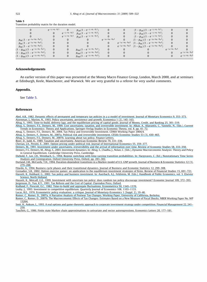
Table 5Transition probability matrix for the duration model.

0 e�kLþaL�bL1 0 pLMð1� e�kLþaL�bL 1Þ 0 0 ð1� pLMÞð1� e�kLþaL�bL1Þ 0 00 0 e�kLþaL�bL 2 pLMð1� e�kLþaL�bL 2Þ 0 0 ð1� pLMÞð1� e�kLþaL�bL2Þ 0 00 0 e�kLþaL�bL 3 pLMð1� e�kLþaL�bL 3Þ 0 0 ð1� pLMÞð1� e�kLþaL�bL3Þ 0 0

pMLð1� e�kMþaM�bM 1Þ 0 0 0 e�kMþaM�bM 1 0 ð1� pMLÞð1� e�kMþaM�bM 1Þ 0 0pMLð1� e�kMþaM�bM 2Þ 0 0 0 0 e�kMþaM�bM 2 ð1� pMLÞð1� e�kMþaM�bM 2Þ 0 0pMLð1� e�kMþaM�bM 3Þ 0 0 0 0 e�kMþaM�bM 3 ð1� pMLÞð1� e�kMþaM�bM 3Þ 0 0

ð1� pHMÞð1� e�kHþaH�bH 1Þ 0 0 pHMð1� e�kHþaH�bH 1Þ 0 0 0 e�kHþaH�bH 1 0ð1� pHMÞð1� e�kHþaH�bH 2Þ 0 0 pHMð1� e�kHþaH�bH 2Þ 0 0 0 0 e�kHþaH�bH 2

ð1� pHMÞð1� e�kHþaH�bH 3Þ 0 0 pHMð1� e�kHþaH�bH 3Þ 0 0 0 0 e�kHþaH�bH 3

522 S. Altug et al. / Journal of Macroeconomics 31 (2009) 509–522

Acknowledgements

An earlier version of this paper was presented at the Money Macro Finance Group, London, March 2000, and at seminarsat Edinburgh, Keele, Manchester, and Warwick. We are very grateful to a referee for very useful comments.

Appendix.

See Table 5.

References

Abel, A.B., 1982. Dynamic effects of permanent and temporary tax policies in a q model of investment. Journal of Monetary Economics 9, 353–373.Aizenman, J., Marion, N., 1993. Policy uncertainty, persistence and growth. Economica 1 (2), 145–163.Altug, S., 1993. Time-to-build, delivery lags, and the equilibrium pricing of capital goods. Journal of Money, Credit, and Banking 25, 301–319.Altug, S., Demers, F.S., Demers, M., 1999. Cost uncertainty, taxation, and irreversible investment. In: Alkan, A., Aliprantis, C., Yannelis, N., (Eds.), Current

Trends in Economics: Theory and Applications. Springer-Verlag Studies in Economic Theory, vol. 8. pp. 41–72.Altug, S., Demers, F.S., Demers, M., 2004. Tax Policy and Irreversible Investment. CDMA Working Paper 2004/4.Altug, S., Demers, F., Demers, M., 2007a. Political risk and irreversible investment. CESifo Economic Studies 53 (3), 430–465.Altug, S., Demers, F.S., Demers, M., 2007b. Learning about tax policy. Finance Letters.Bizer, D., Judd, K., 1989. Taxation and uncertainty. American Economic Review 79, 331–336.Cherian, J.A., Perotti, E., 2001. Option pricing under political risk. Journal of International Economics 55, 359–377.Demers, M., 1991. Investment under uncertainty, irreversibility and the arrival of information over time. Review of Economic Studies 58, 333–350.Demers, F.S., Demers, M., Altug, S., 2003. Investment dynamics. In: Altug, S., Chadha, J., Nolan, C. (Eds.), Dynamic Macroeconomic Analysis: Theory and Policy

in General Equilibrium. Cambridge University Press, Cambridge.Diebold, F., Lee, J.H., Weinbach, G., 1994. Regime switching with time-varying transition probabilities. In: Hargreaves, C. (Ed.), Nonstationary Time Series

Analysis and Cointegration. Oxford University Press, Oxford, pp. 283–302.Durland, J.M., McCurdy, T.H., 1994. Duration-dependent transitions in a Markov model of U.S. GNP growth. Journal of Business & Economic Statistics 12 (3),

279–288.Filardo, A., 1994. Business cycle phases and their transitional dynamics. Journal of Business and Economic Statistics 12, 299–308.Grenadier, S.R., 2002. Option exercise games: an application to the equilibrium investment strategies of firms. Review of Financial Studies 15, 691–721.Hassett, K., Hubbard, G., 2002. Tax policy and business investment. In: Auerbach, A.J., Feldstein, M. (Eds.), Handbook of Public Economics, vol. 3. Elsevier

Science, North Holland.Hassett, K., Metcalf, G.E., 1999. Investment with uncertain tax policy: does random tax policy discourage investment? Economic Journal 109, 372–393.Jorgenson, D., Yun, K.Y., 1991. Tax Reform and the Cost of Capital. Clarendon Press, Oxford.Kydland, F., Prescott, E.C., 1982. Time-to-build and aggregate fluctuations. Econometrica 50, 1345–1370.Leahy, J., 1993. Investment in competitive equilibrium. Quarterly Journal of Economics 108, 1103–1133.Lucas, R.E., 1976. Econometric policy evaluation: a critique. Journal of Monetary-Economics 1 (Suppl. 2), 19–46.Romer, C., Romer, D., 2007a. A Narrative Analysis of Postwar Tax Changes. Working Paper, University of California, Berkeley.Romer, C., Romer, D., 2007b. The Macroeconomic Effects of Tax Changes: Estimates Based on a New Measure of Fiscal Shocks. NBER Working Paper No. WP

13264.Smit, H., Ankum, L., 1993. A real options and game-theoretic approach to corporate investment strategy under competition. Financial Management 22, 241–

250.Tauchen, G., 1986. Finite state Markov chain approximations to univariate and vector autoregressions. Economics Letters 20, 177–181.