A short report about international

carry trade

Fuqi Mao s3465824

Ziwen Hu s3463538

Guohuang Chen s3446218

Jiarui Sui s3464448

i

ii

Table of contents

1. Introduction............................1

2. Theoretical framework...................2

3. Carry trade analysis....................3

3.1.......................Data introduction

3

3.2.....................Model establishment

4

3.3........................Model limitation

5

4. Conclusion..............................7

5. Reference...............................7

iii

1. Introduction

This report is going to verify a specific carry trade

strategy as JPY/AUD in the international finance

market. Given the globalization process advanced, it’s

convenient to transfer from one country’s currency to

another country’s currency. Once the two countries’

fiscal and monetary policies have difference, one

country might have a higher risk free interest rate

than another. If the interest rate gap can be wide

enough to cover the transaction cost and the expected

foreign exchange rate movement, there is a chance to

borrow the low interest rate currency and invest in the

high risk currency to enjoy the interest spread. Such

procedure is called ‘currency carry trade’, or ‘carry

trade’ for simplicity (Galati, Heath & McGuire 2007).

1

Theoretically, the carry trade can be performed between

any two currencies whose countries have different free

interest policies. Today, it has become a popular

trading strategy and attracted many attentions from

financial traders around the world. Many professional

financial information providers like Bloomberg or

financial agents will issue their reports to recommend

the possible carry trade opportunities.

The establishment of carry trade mainly depends on two

factors: the interest yield spread and the exchange

rate movement. Generally, it would be best to borrow

one low interest and depreciating currency to invest

another high interest and appreciating currency, so the

trader can enjoy both the interest and currency premium

2

(Galati, Heath & McGuire 2007). Currently, one possible

carry trade strategy is to borrow JPY to invest in AUD

government bond. From Bloomberg, it’s recommended that

such carry trade strategy can earn premium given the

current interest spread and FX expectation. And once

the trader utilized the leverage, its return will

become much higher. However, such trading strategy

still needs to be under examination before it’s

actually executed.

The following content will be arranged as follows.

After the background introduction, there is a short

explanation for data gathered for analysis. And then a

single equation model for econometric analysis will be

established. It then will be used to forecast the

3

JPY/AUD exchange rate movement in the next 12 months.

Based on the combination of current interest rate and

expected exchange rate movement, it will drawn on the

conclusion about whether and how such carry trade

strategy can provide premium to the trader. Finally,

some limitations and significant risks for such carry

trade strategy will be emphasized. And a short

conclusion will be drawn at the end.

2. Theoretical framework

The carry trade strategy is the result of international

financial market development, which provided a

convenient environment for the cross border transaction

(Levich 2001). With the help of carry trade, the fiscal

and monetary policy difference between various

4

countries will be flattened. In an open international

financial market, one country cannot consider its

fiscal and monetary policy independently without

considering other countries’ reaction, or else the

deviation will be utilized by the arbitrage force from

international traders (Spilimbergo et al 2009).

From the above introduction, it’s obvious that the

success of carry trade depended on two factors as

interest yield spread and the exchange rate movement.

For the short term trading period like 12 months, the

interest from both borrowing and investment can be seen

as relatively fixed (Duffie & Singleton 1997). So the

key thing is left to the exchange rate movement. There

are many theories and models to explain the current and

5

future exchange rate movement like the Covered Interest

Parity (‘CIP’), Purchasing Power Parity (‘PPP’), the

Balance of Payments (‘BoP’) model, partial supply and

demand model, asset market approach and international

Fisher, etc (Obstfeld, Rogoff & Wren-lewis 1996). Each

method cover one or a few important factors to

determine exchange rate movement, but it might also

lack the comprehensiveness to precisely explain the

exchange rate fluctuation.

For example, the CIP argued that the FX rate

fluctuation between the spot rate and forward rate

should equal to the interest rate difference. That is

id- if = Fxt – Fx0. Or else there is an arbitrage opportunity

to make the carry trade. And the PPP explained that the

6

inflation spread shall be the determination of the FX

rate fluctuation. Or else the business man can buy low

and sell high. That is, they will transport the goods

from one country to another to make arbitrage profit.

In this report, it will use the PPP as basic principle

to build the econometric model.

PPP has two versions: absolute PPP and relative PPP

(Obstfeld, Rogoff & Wren-lewis 1996). The absolute PPP

argued that all commercial goods in different countries

should be the same price by exchange rate. That is

Pd/Pf=FX0. But such theory neglected the transaction

cost and other factors like taxation which could make

the price level different.

7

On another version, the relative PPP admitted the

current exchange rate had correctly reflected all

factors available, yet the exchange rate movement can

still be determined by the inflation spread. That it

only predicted the exchange rate movement in future.

That is △P=△FX. Comparing to absolute PPP, the

relative PPP has a more relax assumption and thus has a

stronger explanation power than absolute PPP. And its

effectiveness has been proved by many researchers (Imbs

et al 2005).

3. Carry trade analysis

3.1. Data introduction

Under the PPP theory, the exchange rate can be

forecasted by the expectation of inflation in both

8

countries. Since it’s going to forecast the exchange

rate in 12 months, it’s appropriate to use the annual

data. Per Svensson (1997), inflation is a time series

data which followed a cyclic patter that fluctuated

around the historical average level. Because of that,

it’s needed to collect enough historical data to

identify the cyclic pattern, that in this report it’s

going to use 20 years as the time frame of data.

It’s going to use the consumer price index (‘CPI’) in

Australia and Japan to represent the inflation

situation, which is a commonly used and well

acknowledged indicator to measure the inflation. Both

governments have a complete record of CPI data which

can be retrieved from internet (ABS 2014; Official

9

statistics of Japan 2014).

3.2. Model establishment

Based on the relative PPP theory, the movement of

exchange rate is determined by the inflation difference

between the countries, but there will be some other

factors to affect the exchange rate, too. Because of

that, the initial econometric equation can be drafted

as:

△FX=a+b△P+ ε

Such model assumed that the expected exchange rate

fluctuation is determined by the known inflation

difference between two countries. In the model, there

are two important variables.

10

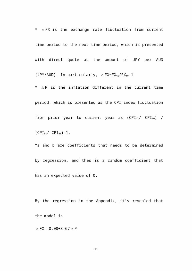
* △FX is the exchange rate fluctuation from current

time period to the next time period, which is presented

with direct quote as the amount of JPY per AUD

(JPY/AUD). In particularly, △FX=FXt1/FXt0-1

* △P is the inflation different in the current time

period, which is presented as the CPI index fluctuation

from prior year to current year as (CPIf1/ CPIf0) /

(CPId1/ CPId0)-1.

*a and b are coefficients that needs to be determined

by regression, and theε is a random coefficient that

has an expected value of 0.

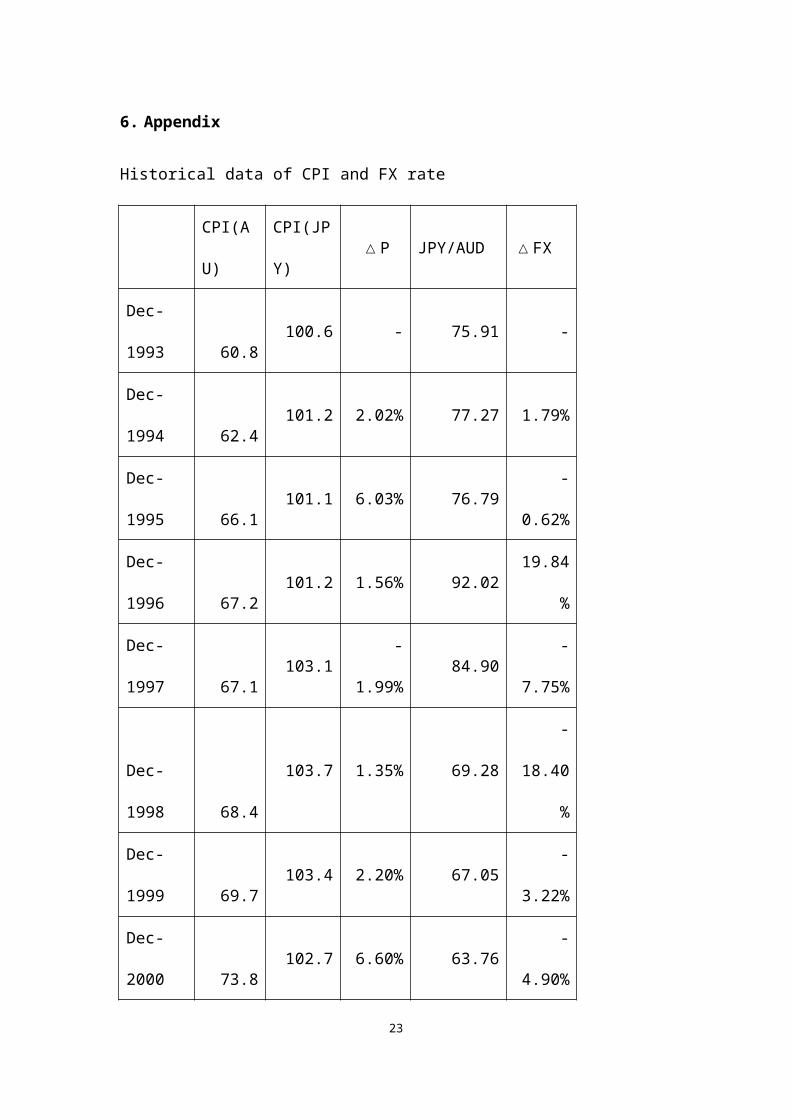
By the regression in the Appendix, it’s revealed that

the model is

△FX=-0.08+3.67△P

11

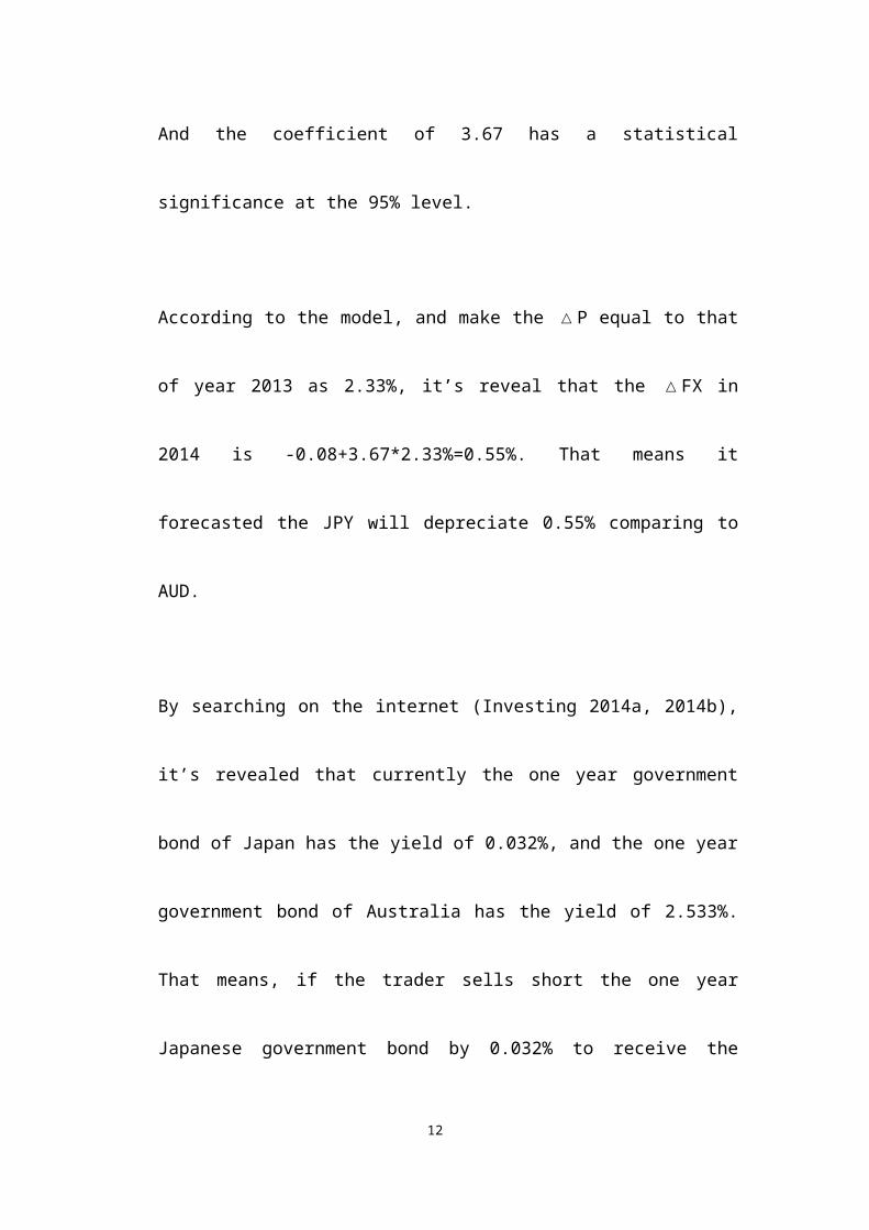
And the coefficient of 3.67 has a statistical

significance at the 95% level.

According to the model, and make the △P equal to that

of year 2013 as 2.33%, it’s reveal that the △FX in

2014 is -0.08+3.67*2.33%=0.55%. That means it

forecasted the JPY will depreciate 0.55% comparing to

AUD.

By searching on the internet (Investing 2014a, 2014b),

it’s revealed that currently the one year government

bond of Japan has the yield of 0.032%, and the one year

government bond of Australia has the yield of 2.533%.

That means, if the trader sells short the one year

Japanese government bond by 0.032% to receive the

12

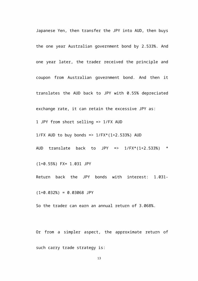
Japanese Yen, then transfer the JPY into AUD, then buys

the one year Australian government bond by 2.533%. And

one year later, the trader received the principle and

coupon from Australian government bond. And then it

translates the AUD back to JPY with 0.55% depreciated

exchange rate, it can retain the excessive JPY as:

1 JPY from short selling => 1/FX AUD

1/FX AUD to buy bonds => 1/FX*(1+2.533%) AUD

AUD translate back to JPY => 1/FX*(1+2.533%) *

(1+0.55%) FX= 1.031 JPY

Return back the JPY bonds with interest: 1.031-

(1+0.032%) = 0.03068 JPY

So the trader can earn an annual return of 3.068%.

Or from a simpler aspect, the approximate return of

such carry trade strategy is:

13

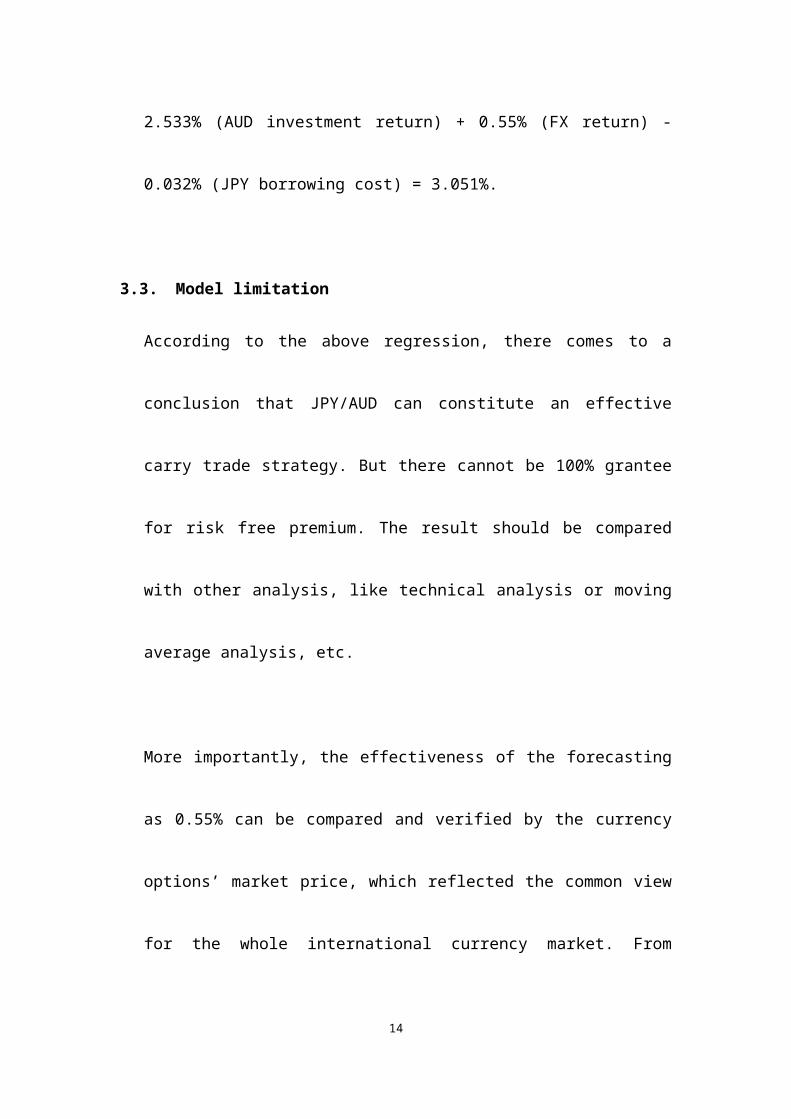
2.533% (AUD investment return) + 0.55% (FX return) -

0.032% (JPY borrowing cost) = 3.051%.

3.3. Model limitation

According to the above regression, there comes to a

conclusion that JPY/AUD can constitute an effective

carry trade strategy. But there cannot be 100% grantee

for risk free premium. The result should be compared

with other analysis, like technical analysis or moving

average analysis, etc.

More importantly, the effectiveness of the forecasting

as 0.55% can be compared and verified by the currency

options’ market price, which reflected the common view

for the whole international currency market. From

14

internet (CMEgroup 2014), it’s revealed that the

current one year option for JPY/AUD in Sep 2015 is

priced at 91.32, that comparing to the current JPY/AUD

as 93.46, JPY is believed to have a 2.28% appreciation

in the next 12 months. Such deviation can be explained

by the following limitations of the econometric model.

First of all, the model’s power can be weaken by the

poor data quality. As a model based on historical data,

its quality is only as good as the input data itself

(Wang & Strong 1996). All the data used for modeling

came from the mass scale statistics, which can be

inaccurate and mistaken. If one or a few data is

mistaken, the regression result might be different. And

that will significantly affect the forecast result. To

15

some extent, it might cause a total different

conclusion because of the different exchange rate

forecasting.

Second, the model assumed that only the relative

inflation can have significant power to affect the

exchange rate movement, that the residual term as ε is

expected to be zero. Such assumption might be wrong.

That in some particular time period, there might be

some other factors to affect the exchange rate, like

the balance of payments. That might result in a

significant deviation between the real value and the

forecasting result.

Most importantly, the regression model is based on the

16

historical data, which only represented the truth of

the past but not the trend in the future (Rousseeuw &

Leroy 2005). Once there comes any new factors in the

future, its consequence cannot be integrated into the

model. One of the new factors is the government

decision, which is not always reasonable and might be

totally unpredictable by the historical data. For

example, in 2013 the Abe regime has begun to execute a

new round of simulative package which has not been

performed before (Ujikane & Otsuma 2013). Such new

policy was not reflected by the historical data before

2013, so its consequence to the JPY currency will also

be out of the prediction range of the regression model.

Because of the deviation of current option quotes and

17

volatile of the governmental policy from Japan, it

might be keep alert before executing the JPY/AUD carry

trade.

4. Conclusion

In conclusion, the development of international

currency market has provided many chances in the cross

border investment. The carry trade strategy is to use

the low interest cost currency to invest in high

interest currency to earn premium. The key to the

success of carry trade strategy is to correctly

forecast the foreign exchange rate in the future. For

one possible strategy as JPY/AUD carry trade, it

collected the relative PPP theoretical framework by

historical inflation data in Japanese and Australia.

18

And then it regressed their relations with the JPY/AUD

exchange rate fluctuation, as well as trying to

forecast the exchange rate in the next 12 months. The

regression and forecast result supported the carry

trade strategy, while the market price of currency

option has quite a deviation from the forecast result.

Given the econometric model might have several

limitations, it had better to review the strategy again

with other supplemental analysis.

19

5. Reference

ABS 2014, 6401.0 - Consumer Price Index, viewed 11th Otc 2014,

<http://www.abs.gov.au/AUSSTATS/abs@.nsf/DetailsPage/

6401.0Jun%202014?OpenDocument>.

CMEgroup 2014, Australian Dollar/Japanese Yen Futures Quotes, viewed

11th Otc 2014,

<http://www.cmegroup.com/trading/fx/g10/australian-

dollar-japanese-yen.html>.

Duffie, D & Singleton, KJ 1997, ‘An econometric model of

the term structure of interest‐rate swap yields’, The

Journal of Finance, vol.52, no.4, pp.1287-1321.

Galati, G, Heath, A & McGuire, P 2007, ‘Evidence of carry

trade activity’, BIS Quarterly Review, vol.3,no.1, pp.27-41.

20

Imbs, J, Mumtaz, H, Ravn, MO & Rey, H 2005, ‘PPP strikes

back: Aggregation and the real exchange rate’, The quarterly

journal of economics, vol.120, no.1,pp.1-43.

Investing 2014a, Australia 1-Year Bond Yield, viewed 11th Otc

2014,

< http://www.investing.com/rates-bonds/australia-1-year-

bond-yield>.

Investing 2014b, Japan 1-Year Bond Yield, viewed 11th Otc 2014,

< http://www.investing.com/rates-bonds/japan-1-year-bond-

yield>.

Levich, RM 2001, International financial markets. McGraw-Hill,

Irwin.

Obstfeld, M, Rogoff, KS & Wren-lewis, S 1996, Foundations of

international macroeconomics. MIT press, Cambridge.

Official statistics of Japan 2014, 2010-Base Consumer Price

Index, viewed 11th Otc 2014,

<http://www.e-stat.go.jp/SG1/estat/ListE.do?

21

bid=000001033700&cycode=0>.

Rousseeuw, PJ & Leroy, AM 2005, Robust regression and outlier

detection. John Wiley & Sons, New York.

Spilimbergo, MA, Symansky, MSA, Cottarelli, MC &

Blanchard, OJ 2009, Fiscal policy for the crisis. International

Monetary Fund, New York.

Svensson, LE 1997, ‘Inflation forecast targeting:

Implementing and monitoring inflation targets’, European

economic review, vol.41, no.6, pp. 1111-1146.

Ujikane, K & Otsuma, M 2013, Japan’s Abe unveils 10.3 trillion Yen

fiscal stimulus,viewed 10th Oct 2014,

<http://www.bloomberg.com/news/2013-01-11/japan-s-abe-

unveils-10-3-trillion-yen-fiscal-boost-to-growth.html>.

Wang, RY & Strong, DM 1996, ‘Beyond accuracy: What data

quality means to data consumers’, Journal of management

information systems, vol. 12, no.4, pp. 5-33.

22

6. Appendix

Historical data of CPI and FX rate

CPI(A

U)

CPI(JP

Y)△P JPY/AUD △FX

Dec-

1993 60.8100.6 - 75.91 -

Dec-

1994 62.4101.2 2.02% 77.27 1.79%

Dec-

1995 66.1101.1 6.03% 76.79

-

0.62%

Dec-

1996 67.2101.2 1.56% 92.02

19.84

%

Dec-

1997 67.1103.1

-

1.99%84.90

-

7.75%

Dec-

1998 68.4

103.7 1.35% 69.28

-

18.40

%

Dec-

1999 69.7103.4 2.20% 67.05

-

3.22%

Dec-

2000 73.8102.7 6.60% 63.76

-

4.90%

23

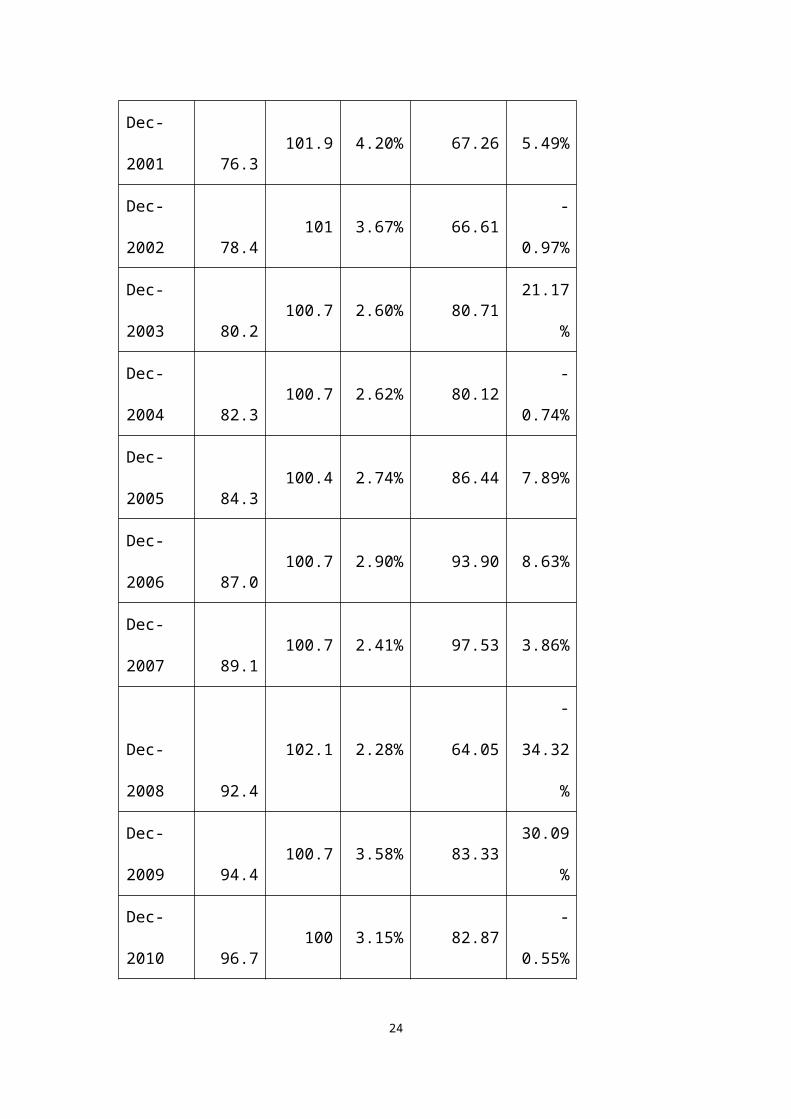
Dec-

2001 76.3101.9 4.20% 67.26 5.49%

Dec-

2002 78.4101 3.67% 66.61

-

0.97%

Dec-

2003 80.2100.7 2.60% 80.71

21.17

%

Dec-

2004 82.3100.7 2.62% 80.12

-

0.74%

Dec-

2005 84.3100.4 2.74% 86.44 7.89%

Dec-

2006 87.0100.7 2.90% 93.90 8.63%

Dec-

2007 89.1100.7 2.41% 97.53 3.86%

Dec-

2008 92.4

102.1 2.28% 64.05

-

34.32

%

Dec-

2009 94.4100.7 3.58% 83.33

30.09

%

Dec-

2010 96.7100 3.15% 82.87

-

0.55%

24

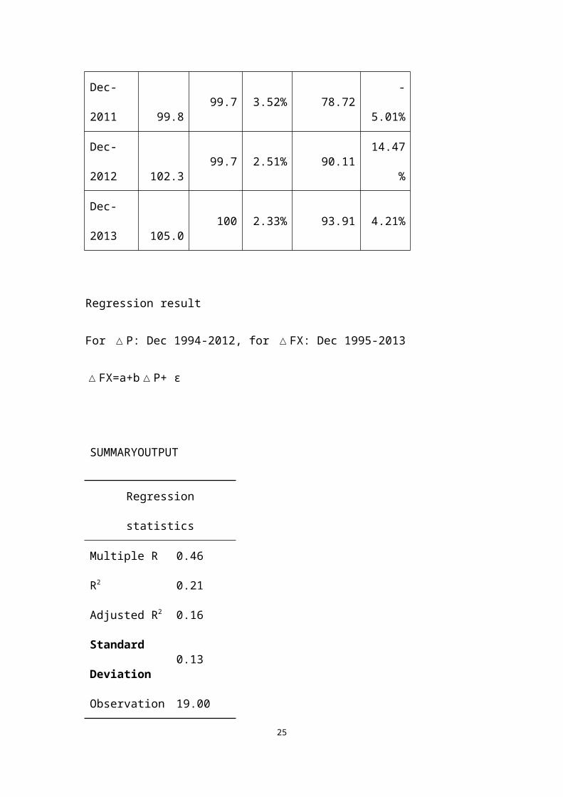
Dec-

2011 99.899.7 3.52% 78.72

-

5.01%

Dec-

2012 102.399.7 2.51% 90.11

14.47

%

Dec-

2013 105.0100 2.33% 93.91 4.21%

Regression result

For △P: Dec 1994-2012, for △FX: Dec 1995-2013

△FX=a+b△P+ ε

SUMMARYOUTPUT

Regression

statistics

Multiple R 0.46

R2 0.21

Adjusted R2 0.16

Standard

Deviation0.13

Observation 19.00

25

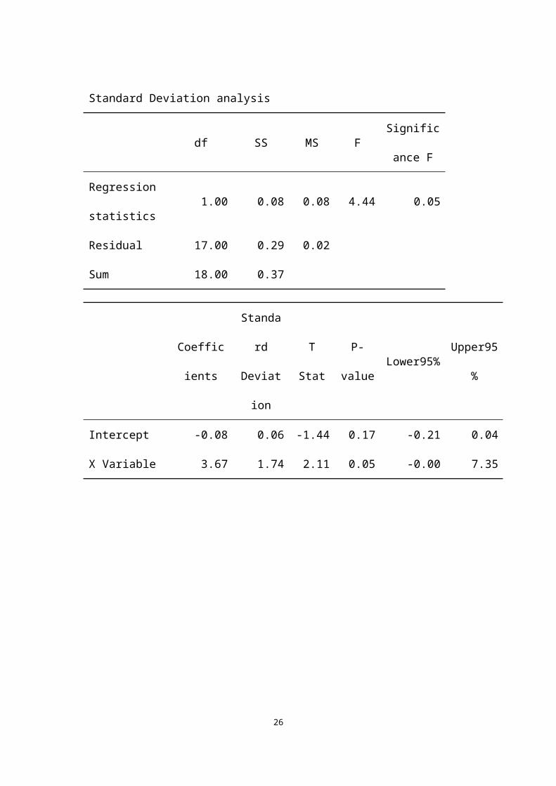
Standard Deviation analysis

df SS MS FSignific

ance F

Regression

statistics1.00 0.08 0.08 4.44 0.05

Residual 17.00 0.29 0.02

Sum 18.00 0.37

Coeffic

ients

Standa

rd

Deviat

ion

T

Stat

P-

valueLower95%

Upper95

%

Intercept -0.08 0.06 -1.44 0.17 -0.21 0.04

X Variable 3.67 1.74 2.11 0.05 -0.00 7.35

26