Embed Size (px)
Citation preview

Managerial FinanceReal estate investingGuest Editor: Don T. Johnson
Volume 32 Number 12 2006
ISSN 0307-4358
www.emeraldinsight.com
mf cover (i).qxd 09/10/2006 08:36 Page 1

Access this journal online _________________________ 951
Editorial advisory board___________________________ 952
GUEST EDITORIAL
Real estate investingDon T. Johnson________________________________________________ 953
Mean-variance analysis with REITs in mixed assetportfolios: the return interval and the time periodused for the estimation of inputsDoug Waggle and Gisung Moon __________________________________ 955
The turn-of-the-month effect in real estateinvestment trusts (REITs)William S. Compton, Don T. Johnson and Robert A. Kunkel____________ 969
REIT capital structure: is it market imposed?K. Michael Casey, Glenna Sumner and James Packer _________________ 981
Managerial Finance
Real estate investing
Guest EditorDon T. Johnson
ISSN 0307-4358
Volume 32Number 122006
CONTENTS
The current and past volumes of this journal are available at:
www.emeraldinsight.com/0307-4358.htmYou can also search more than 100 additional Emerald journals inEmerald Fulltext (www.emeraldinsight.com/ft) and EmeraldManagement Xtra (www.emeraldinsight.com/emx)
See page following contents for full details of what your access includes.
Access this journal electronically

Manager characteristics and real estate mutual fundreturns, risk and feesJames Philpot and Craig A. Peterson_______________________________ 988
The strong building: a case study in directinvestmentWalt A. Nelson ________________________________________________ 997
CONTENTScontinued

As a subscriber to this journal, you can benefit from instant,electronic access to this title via Emerald Fulltext or EmeraldManagement Xtra. Your access includes a variety of features thatincrease the value of your journal subscription.
How to access this journal electronicallyTo benefit from electronic access to this journal, please [email protected] A set of login details will then beprovided to you. Should you wish to access via IP, pleaseprovide these details in your e-mail. Once registration iscompleted, your institution will have instant access to all articlesthrough the journal’s Table of Contents page atwww.emeraldinsight.com/0307-4358.htm More informationabout the journal is also available at www.emeraldinsight.com/mf.htm
Our liberal institution-wide licence allows everyone within yourinstitution to access your journal electronically, making yoursubscription more cost-effective. Our web site has beendesigned to provide you with a comprehensive, simple systemthat needs only minimum administration. Access is available viaIP authentication or username and password.
Key features of Emerald electronic journals
Automatic permission to make up to 25 copies of individualarticlesThis facility can be used for training purposes, course notes,seminars etc. This only applies to articles of which Emerald ownscopyright. For further details visit www.emeraldinsight.com/copyright
Online publishing and archivingAs well as current volumes of the journal, you can also gainaccess to past volumes on the internet via Emerald Fulltext orEmerald Management Xtra. You can browse or search thesedatabases for relevant articles.
Key readingsThis feature provides abstracts of related articles chosen by thejournal editor, selected to provide readers with current awarenessof interesting articles from other publications in the field.
Non-article contentMaterial in our journals such as product information, industrytrends, company news, conferences, etc. is available online andcan be accessed by users.
Reference linkingDirect links from the journal article references to abstracts of themost influential articles cited. Where possible, this link is to thefull text of the article.
E-mail an articleAllows users to e-mail links to relevant and interesting articles toanother computer for later use, reference or printing purposes.
Structured abstractsEmerald structured abstracts provide consistent, clear andinformative summaries of the content of the articles, allowingfaster evaluation of papers.
Additional complimentary services availableYour access includes a variety of features that add to thefunctionality and value of your journal subscription:
E-mail alert servicesThese services allow you to be kept up to date with the latestadditions to the journal via e-mail, as soon as new materialenters the database. Further information about the servicesavailable can be found at www.emeraldinsight.com/alerts
ConnectionsAn online meeting place for the research community whereresearchers present their own work and interests and seek otherresearchers for future projects. Register yourself or search ourdatabase of researchers at www.emeraldinsight.com/connections
Emerald online training servicesYou can also access this journal online. Visitwww.emeraldinsight.com/training and take an Emerald onlinetour to help you get the most from your subscription.
Choice of accessElectronic access to this journal is available via a number ofchannels. Our web site www.emeraldinsight.com is therecommended means of electronic access, as it provides fullysearchable and value added access to the complete content ofthe journal. However, you can also access and search the articlecontent of this journal through the following journal deliveryservices:
EBSCOHost Electronic Journals Serviceejournals.ebsco.com
Informatics J-Gatewww.j-gate.informindia.co.in
Ingentawww.ingenta.com
Minerva Electronic Online Serviceswww.minerva.at
OCLC FirstSearchwww.oclc.org/firstsearch
SilverLinkerwww.ovid.com
SwetsWisewww.swetswise.com
Emerald Customer SupportFor customer support and technical help contact:E-mail [email protected] www.emeraldinsight.com/customercharterTel +44 (0) 1274 785278Fax +44 (0) 1274 785204
www.emeraldinsight.com/mf.htm

MF32,12
952
Managerial FinanceVol. 32 No. 12, 2006p. 952#Emerald Group Publishing Limited0307-4358
EDITORIAL ADVISORY BOARD
Professor Kofi A. AmoatengNC Central University, Durham, USA
Professor Felix AyadiJesse E. Jones School of Business, Texas SouthernUniversity, USA
Professor Mohamed E. BayouThe University of Michigan-Dearborn, USA
Dr Andre de KorvinUniversity of Houston-Downtown, USA
Dr Colin J. DoddsSaint Mary’s University, Halifax, Nova Scotia,Canada
Professor John DoukasOld Dominion University, Norfolk, Virginia, USA
Professor Uric DufreneIndiana University Southeast, New Albany,Indiana, USA
Professor Ali M. FatemiDe Paul University, Chicago, Illinois, USA
Professor Iftekhar HasanNew Jersey Institute of Technology, USA
Professor Suk H. KimUniversity of Detroit Mercy, Detroit, USA
Professor John LeavinsUniversity of Houston-Downtown, USA
Professor R. Charles MoyerWake Forest University, Winston-Salem, NorthCarolina, USA
Dr Khursheed OmerUniversity of Houston-Downtown, USA
Professor Moses L. PavaYeshiva University, New York, USA
Professor George C. PhilipatosThe University of Tennessee, Knoxville, Tennessee,USA
Professor David RayomeNorthern Michigan University, USA
Professor Alan ReinsteinWayne State University, Detroit, Michigan, USA
Professor Ahmed Riahi-BelkaouiThe University of Illinois at Chicago, USA
Professor Mauricio RodriguezTexas Christian University, Fort Worth, Texas,USA
Professor Salil K. SarkarHenderson State University, Arkadelphia,Arkansas, USA
Professor Atul A. SaxenaMercer University, Georgia, USA
Professor Philip H. SiegelMonmouth University, New Jersey, USA
Professor Kevin J. SiglerThe University of North Carolina at Wilmington,USA
Professor Gordon WillsInternational Management Centres, UK
Professor Stephen A. ZeffRice University, Texas, USA

Real estateinvesting
953
Managerial FinanceVol. 32 No. 12, 2006
pp. 953-954# Emerald Group Publishing Limited
0307-4358DOI 10.1108/03074350610710445
GUEST EDITORIAL
Real estate investingDon T. Johnson
Department of Finance, Western Illinois University,Macomb, Illinois, USA
Abstract
Purpose – Aims to explain the rationale for producing an issue on the topic of real estate investingand how these articles fit together.Design/methodology/approach – Essay format.Findings – Real estate is probably the largest category of assets for investors and the works in thisissue will assist in the decision making processes of real estate investors.Research limitations/implications – Each of these papers covers only a limited topic and moreresearch in the area is needed.Practical implications – These papers could change how asset allocation studies are conducted;allow investors to make superior returns around the turn of the month on real estate investmenttrusts (REITs); alter the capital structure of REITs; seek out real estate mutual funds with highermanagement fees (because they were associated with higher returns); invest directly in real estateproperties.Originality/value – All five of these papers either examine areas that have not been reviewed byresearchers previously, or find results that may result in different investment decisions.
Keywords Real estate, Assets management, Investments
Paper type Viewpoint
This issue of Managerial Finance is dedicated to the study of real estate investments.Real estate accounts for approximately two-thirds of the national wealth of the UnitedStates and over 25 per cent of the gross domestic product. Experts attribute about 25per cent of the worth of publicly traded corporations to their investments in real estate.Recent studies by the Census Bureau and other organizations have identified real estateas the largest holding for a large percentage of households in the United States. Clearly,issues surrounding real estate investing are of considerable interest to many partiesincluding individual investors, institutional investors and even corporations who ownreal estate as part of their operations. I believe that these and other parties will find thearticles in this issue to be notably useful in their real estate decision making.
In the first article in this issue, Waggle and Moon (2006) examine how using variousreturn intervals affect optimal portfolio allocation decisions where the portfolio maycontain real estate investment trusts (REITs). Much asset allocation research has beenpublished but different studies often arbitrarily select different return intervals.Waggle andMoon (2006) show, at least with regards to REITs, that changing the returnperiod from an annual interval to semiannual, quarterly or monthly can dramaticallychange the optimal portfolio allocation recommendations in substantial part due tosystematically understated annual volatility. By challenging the haphazard selection ofreturn intervals, the Waggle and Moon (2006) work may change how asset allocationdecisions are made in the future.
The second paper by Compton et al. (2006), examines both equity and mortgageREIT returns around the turn of the month (TOM). We employ a battery of bothparametric and nonparametric statistical tests that address the concerns ofdistributional violations raised in previous studies. The results reveal dramatic andsignificant positive returns on REIT stocks around the TOM. The results may indicate
The current issue and full text archive of this journal is available atwww.emeraldinsight.com/0307-4358.htm

MF32,12
954
an opportunity for investors to help bring efficiency to the market by making andtaking profits in REIT stocks around the TOM.
Casey et al. (2006) scrutinize the capital structure of REITs in the third paper of thisissue. Using REITs as a proxy for nontax-driven capital structure decisions (since theyavoid corporate taxation by paying out most of their earnings), they find evidence thatREITs’ capital structures are influenced by various market factors such as price-to-book ratios, institutional ownership and price-to-cash flow ratios. Further, they findthat different types of REITs utilize different capital structures. Managers andinvestors may be able to use the information in this article to optimize REIT values.
The fourth paper by Philpot and Peterson (2006) examines how the characteristics ofthe managers of real estate mutual funds are associated with the funds’ performances,risk levels andmanagement fees. Contrary tomuch research using non-real estate mutualfunds, Philpot and Peterson (2006) find that real estate funds with higher managementfees produce higher fund returns. They also find that team-managed funds have lowerreturns and that there is little evidence of returns being positively related to a manager’sexperience or certification. The Philpot and Peterson (2006) results differ in several waysfrom those most commonly found by researchers studying the broad mutual fundindustry and thus researchers and investors in the specialized real estate mutual fundsmay find their work to be quite informative and useful.
Finally, Nelson (2006) explores the topic of direct real estate investing which, despitethe popularity and high profile of indirect investing vehicles such as REITs, is still themost common avenue for individuals and institutions to add real estate exposure to theirportfolios. Nelson (2006) discusses the comparative advantages and problems of directreal estate investing vis-a-vis indirect investing. He then takes us through an actualinvestment case involving a mixed use building in the upperMidwestern United States.
Many thanks go to Dr Richard Dobbins for offering me the opportunity to assemblethis issue of Managerial Finance. Additional thanks go to Michael Casey for acting asSpecial Editor on my article with William Compton and Robert Kunkel. Finally, Iespecially want to thank the numerous anonymous reviewers who gave of their timeand effort to read and screen the submissions for this issue. They identified the bestpapers among the works submitted and then improved the papers in this issue byrecognizing problems and suggesting ways for the authors to improve their articles.
References
Casey, M., Sumner, G. and Packer, J. (2006), ‘‘REIT capital structure: is it market imposed?’’,Managerial Finance, Vol. 32.
Compton, W., Kunkel, R. and Johnson, D. (2006), ‘‘The turn-of-the-month effect in real estateinvestment trusts (REITs)’’,Managerial Finance, Vol. 32.
Nelson, W. (2006), ‘‘The strong building: a case study in direct investment’’, Managerial Finance,Vol. 32.
Philpot, J. and Peterson, C. (2006), ‘‘Manager characteristics and real estate mutual fund returns,risk and fees’’,Managerial Finance, Vol. 32.
Waggle, D. and Moon, G. (2006), ‘‘Mean-variance analysis with REITs in mixed asset portfolios:the return interval and the time period used for the estimation of inputs’’, ManagerialFinance, Vol. 32.

Mean-varianceanalysis
955
Managerial FinanceVol. 32 No. 12, 2006
pp. 955-968# Emerald Group Publishing Limited
0307-4358DOI 10.1108/03074350610710454
Mean-variance analysis withREITs in mixed asset portfoliosThe return interval and the time period
used for the estimation of inputs
Doug WaggleDepartment of Accounting and Finance, University of West Florida,
Pensacola, Florida, USA, and
Gisung MoonBerry College, Mount Berry, Georgia, USA
Abstract
Purpose – Aims to test to determine whether the selection of the historical return time interval(monthly, quarterly, semiannual, or annual) used for calculating real estate investment trust (REIT)returns has a significant effect on optimal portfolio allocations.Design/methodology/approach – Using a mean-variance utility function, optimal allocations toportfolios of stocks, bonds, bills, and REITs across different levels of assumed investor risk aversion arecalculated. The average historical returns, standard deviations, and correlations (assuming differenttime intervals) of the various asset classes are used as mean-variance inputs. Results are also comparedusing more recent data, since 1988, with, data from the full REIT history, which goes back to 1972.Findings – Using the more recent REIT datarather than the full dataset results in optimal allocationsto REITs that are considerably higher. Likewise, using monthly and quarterly returns tends tounderstate the variability of REITs and leads to higher portfolio allocations.Research limitations/implications – The results of this study are based on the limited historicalreturn data that are currently available for REITs. The results of future time periods may not prove tobe consistent with the findings.Practical implications – Numerous research papers arbitrarily decide to employ monthly orquarterly returns in their analyses to increase the number of REIT observations they have available.These shorter interval returns are generally annualized. This paper addresses the consequences ofthose decisions.Originality/value – It has been shown that the decision to use return estimation intervals shorter thana year does have dramatic consequences on the results obtained and, therefore, must be carefullyconsidered and justified.
Keywords Assets management, Real estate, Returns
Paper type Research paper
IntroductionEstimates of the means and standard deviations of security returns and thecorrelations of those return series are essential to many portfolio decisions. Investorstypically use historical calculations of this return series data as proxies for expectedvalues. In widely used mean-variance analysis, historical return series data isemployed to determine optimal portfolio allocations to various assets or asset classes.With mean-variance analysis investors can determine portfolio weights that maximizereturns for given risk levels or that minimize risk for given return levels.
Despite the widespread use of historical data related to asset returns, there are nohard and fast rules as to exactly how these historical figures should be determined.Many researchers will base calculations on annual return series, but others mayarbitrarily use monthly or quarterly data in order to gain more observation points.
The current issue and full text archive of this journal is available atwww.emeraldinsight.com/0307-4358.htm

MF32,12
956
Some researchers use the entire historical return series available, while others mayargue that one particular time period is more applicable than another.
The primary focus of our paper pertains to portfolio choices relating to equity realestate investment trusts (EREITs) in mixed-asset portfolios. Using mean-varianceanalysis with stocks, bonds, cash, and EREITs, we test to see if using return data(means, standard deviations, and correlation coefficients) calculated from differentreturn intervals (monthly, quarterly, semiannul, and annual) affects optimal portfolioallocations. If, for instance, using monthly or quarterly vs annual returns (over thesame historical time period) to calculate mean-variance inputs has no impact onoptimal portfolio allocations, then researchers should feel comfortable using theshorter return intervals with the resulting additional observations. If, on the otherhand, using shorter return intervals has a significant impact on the portfolioallocations, researchers should provide support for their return interval choice. This is,particularly, applicable if the return interval used for estimation purposes differs fromthe estimated holding period. The available historical return data for real estateinvestment trusts (REITs) is very limited compared to that of stocks, bonds, and cash,but many argue that the more recent observations are more relevant due to theevolution of REITs over time. For our analysis, we also examine the impact on mean-variance efficient portfolios if return series data is derived from the full history ofEREITs as compared to the more recent time period.
The rest of the paper continues as follows: The next section provides somebackground on REITs and examines their place in the portfolio, as well as the impactsof the time interval on correlations, standard deviations and betas. After that wediscuss our data and the basic statistics we calculated. Included in this section are theannual and annualized mean and standard deviation calculations, as well ascorrelation matrices calculated using different return intervals. In our methodologysection, we explain the mean-variance utility function that we employ. Our results andanalysis are followed by our conclusions.
Literature reviewREITsREITs are corporations with a special tax classification that allows them to avoidpaying taxes on their earnings as long as certain criteria are met. REITs must invest ineither direct ownership of real estate or in financing of real estate by holdingmortgages. These corporations must also distribute at least 90 per cent of theirearnings to their shareholders each year as dividends. Shareholders then pay theirtaxes at their individual income tax rates. The vast majority of REITs are EREITswhich own and operate income producing real estate. Mortgage REITs either lendmoney directly to real estate owners or purchase mortgages or mortgage-backedbonds. Hybrid REITs are involved in a combination of real estate ownership andfinancing. The National Association of Real Estate Investment Trusts (NAREIT)provides more information on REITs at www.nareit.com.
REITs are also called real estate stocks and were created to give small investorsthe opportunity to invest in large commercial properties. Corgel et al. (1995) suggestthat real estate literature supports the notion that REITs incorporate some of thecharacteristics of both real estate and stock. Liang (1998) shows that REITs historicallybehaved similarly to a portfolio of 40 per cent small capitalization stocks and 60 per centbonds, but that REITs became more unique over the last five years of his study period.Peterson and Hsieh (1997) find that EREIT returns were related to risk premiums on

Mean-varianceanalysis
957
common stocks. Ziering et al. (1999) noted a downward trend in the correlation betweenstocks and REITs, which they expected to continue. Seiler et al. (1999) go as far as tosuggest that private real estate and EREITs behave differently and should be treatedas entirely separate asset classes. Seiler et al. (2001) further show that EREITs are notsuitable for rebalancing or diversifying private real estate portfolios. Clayton andMacKinnon (2001), on the other hand, found that in the 1990s REIT returns wereclosely linked to the real estate asset class suggesting that they may be an acceptablesubstitute for real estate in the portfolio. One of the major differences between REITreturns and those of private real estate is that while the returns of REITs are based onmarket prices, return series for private real estate are generally based on appraisals.Gyourko and Keim (1993) suggested that the market-based returns of REITs actuallycapture information about changes in real estate values ahead of the returns derivedfrom appraisals.
Real estate and REITs in the portfolioReal estate has a definite role in the portfolios of institutions and individuals. There aremany works such as Fogler (1984), Firstinberg et al. (1988), Ennis and Burik (1991), andKallberg et al. (1996) which suggest optimal allocations to real estate of approximately10 to 20 per cent of the overall investment portfolio. On the opposite end of thespectrum, Webb et al. (1988) argue that two-thirds of investment wealth should beallocated to real estate with the remainder going to financial assets such as stocks andbonds. Giliberto (1992) employs mean-variance analysis to show that if gross realestate returns ranged from 10 to 12 per cent, then portfolio allocations to real estate of5-15 per cent could be justified. Bajtelsmit and Worzala (1995) examine 159 pensionfunds and find actual allocations to real estate that ranged from 0 to 17 per cent with anaverage allocation of only 4.4 per cent. Ziering and McIntosh (1997) and Hudson-Wilson (2001) both show that public real estate (REITs) and private real estate providesignificant diversification benefits in mixed asset portfolios. Waggle and Johnson(2003) consider a single family home to be a key real estate component of an individualinvestor’s portfolio and examine the affects on allocations to the traditional portfolio.Goodman (2003) and Waggle and Johnson (2004) demonstrate that REITs providediversification benefits to individual investors when the family home is considered asan asset.
Correlations, returns, and standard deviationsThe returns, standard deviations, and correlation coefficients of asset classes allchange over time. Ziering and McIntosh (1997) observe that the relationships betweenthe S&P 500, long-term government bonds, REITs, and real estate changeddramatically over their 1972-1995 study period. Dopfel (2003) likewise sawconsiderable changes between the correlations of stocks and bonds from 1929 throughJune 2003. While the typical stock-bond correlation coefficient is assumed to be about+0.4, Dopfel notes many three-year periods where the correlation was actuallynegative. Waggle and Moon (2005) prove the importance of the stock-bond correlationon asset allocation decisions. Wainscott (1990) derives stock-bond correlationcoefficients using rolling one, three, five, and ten-year periods. Not surprisingly, theswings in the one-year correlations are much larger, but there were still periods whereeven the ten-year correlations are negative.
We found very few works examining the use of different return intervals incalculating correlation coefficients. Levy et al. (2001) note that with serial correlation,

MF32,12
958
the time interval selected for calculating correlation coefficients may affect the results.Levy et al. also show that when one variable is multiplicative and the other is additivethe choice of return interval used can impact the correlation coefficient calculationseven if all random variables are independent over time. When both variables aremultiplicative as in our study, Levy and Schwartz (1997) suggest that the correlationcoefficient decreases as the time interval increases. For example, the correlationcoefficient for a pair of independent assets decreases if quarterly returns are usedinstead of monthly returns in the calculation or if annual returns are used instead ofquarterly returns.
Giliberto (2003) used the National Council of Real Estate Investment Fiduciaries(NCREIF) property index to show that when there is significant, positiveautocorrelation in the return series, using monthly or quarterly returns to estimateannual variability would lead to understatement of the volatility of the asset class.NCREIF’s quarterly returns had a very high 0.68 serial correlation, based on one-monthlagged returns. Annualizing the quarterly standard deviation of the NCREIF propertyindex suggests an annual standard deviation of 3.4 per cent. Giliberto’s simulationwork shows that the actual annual volatility is more likely to be in the 7 per cent to 8per cent range. In this case annualized quarterly figures understate volatility by morethen 50 per cent. Giliberto suggests that this should not be an issue with stocks sincethey have low serial correlation of 0.03.
The calculation of a security’s beta includes the correlation of the security with themarket portfolio, so some of the literature on beta applies to our analysis. In the case ofbeta, as with correlation coefficients, there seem to be arbitrary decisions regarding thereturn interval and the estimation time period to be used. Lamb and Northington (2001)surveyed various data sources to determine their methods for calculating securitybetas. Value Line and Standard and Poor’s use a five-year calculation window, whileBloomberg uses only a two-year estimation period. While the use of monthly returns incalculating beta is the norm, Value Line and Bloomberg both use weekly returns, whileBridge and Argus use daily returns.
Levhari and Levy (1977) provide a theoretical examination of betas assumingdifferent return intervals in their calculations. They find that for betas less than one,longer interval betas are higher than shorter interval betas (for example, monthly vsdaily betas). For betas greater than one, they believe the opposite to be true. Theirconclusions are supported by the empirical work of Levy (1984), but challenged byempirical works by Hawawini and Vora (1981) and Saniga et al. (1981). Hawawini andVora (1982) calculated betas with several different methodologies and using daily,weekly, biweekly, and monthly returns and compared their calculated prior periodbetas to daily betas calculated from the subsequent 600 days. Prior period betascalculated based on daily returns were found to have the highest correlation with thesubsequent betas. Reilly and Wright (1988) compared Value Line’s weekly betas toMerrill Lynch’s monthly betas and concluded that there were differences between thetwo related to the return interval used and security size factors. Chang and Weiss(1991) found differences between quarterly and semi-annual betas. Groenewold andFraser (2000) compared a two-year beta estimation period to the standard five-yearestimation period and concluded that the latter provided more useful estimates.
Data and basic statisticsWe employ monthly, quarterly, semiannual, and annual historical return data forEREITs, large-company stocks, long-term government bonds, and treasury bills for

Mean-varianceanalysis
959
the 1972-2002 period. Rather than mixing mortgage and equity REITs in our analysis,we chose to focus exclusively on the more common EREITs. The 1972 start date isconstrained by the availability of EREIT returns. We obtained total returns (capitalgains and dividends) of large company stocks, long-term government bonds, and UStreasury bills from Ibbotson Associate’s SBBI 2003 Yearbook. Hereafter, we will referto them simply as stocks, bonds, and cash, respectively. We use the total return data forEREITs obtained from the NAREIT.
After calculating means and standard deviations based on monthly, quarterly, andsemiannual returns, we annualized all of the estimates. The annualized return rA iscalculated as follows:
rA ¼ ð1þ rnÞn � 1 ð1Þ
where rn is mean return for the return interval and n is the number of periods there areper year. The commonly used annualized standard deviation �A calculated is as follows:
�A ¼ffiffiffin
p�n ð2Þ
where �n is the standard deviation of the return interval. The multi-period standarddeviation calculation assumes that each period’s returns are independent and identicallydistributed.
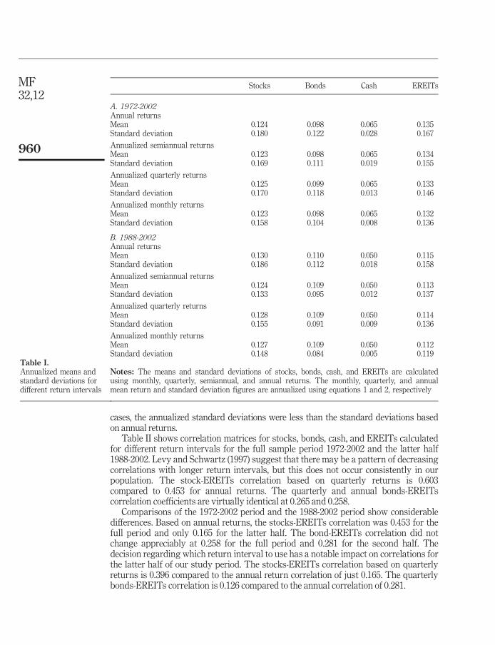
Table I, panel A shows the means and standard deviations of the returns of stocks,bonds, cash, and EREITs for the full 1972-2002 period. The first set of figures showsthe calculations based on annual returns and then there are annualized calculationsbased on semiannual, quarterly, and monthly returns as described above. Based onannual returns, stocks have a mean return of 12.4 per cent and a standard deviation of18.0 per cent. The mean and standard deviation of bonds are 9.8 and 12.2 per cent,respectively. The mean return for cash is 6.5 per cent with a standard deviation of 2.8per cent. For the full period EREITs are the dominant asset with a higher return thanstocks and a lower standard deviation. EREITs had a mean return of 13.5 per cent anda standard deviation of 16.7 per cent.
The annualized mean returns differ only trivially from the annual means, but this isnot the case for the annualized standard deviations. The annualized standard deviationcalculations all understate their annual counterparts. The standard deviationcalculations for EREITs and cash both increase steadily as the return intervalincreases. This could be explained by a lack of independence of the various returnseries as noted by Giliberto (2003). Lagged monthly stock returns are, however,virtually uncorrelated with a serial correlation figure of �0.014. The serial correlationfigures for bonds, cash, and EREITs are all positive with values of 0.081, 0.941, and0.109, respectively. Some of the differences between the annualized and annualcalculations are consistent with the Levhari and Levy (1977) observations on beta. Thehigh serial correlation of cash explains the striking differences between the annualizedstandard deviations and the standard deviation of the annual returns. The monthlyannualized standard deviation for cash is 0.008 compared to the standard deviation ofannual returns of 0.028.
Observations for the second half of our study period 1988 through 2002 arecomparable to the full sample. It is notable that EREITs no longer dominate stocks in thissample period. EREITs have less risk than stocks, but they also have a lower return. Themean return of EREITs was 11.5 per cent compared to 13.0 per cent for stocks. Thestandard deviations of stocks and EREITs were 18.6 and 15.8 per cent, respectively. In all
MF32,12
960
cases, the annualized standard deviations were less than the standard deviations basedon annual returns.
Table II shows correlation matrices for stocks, bonds, cash, and EREITs calculatedfor different return intervals for the full sample period 1972-2002 and the latter half1988-2002. Levy and Schwartz (1997) suggest that there may be a pattern of decreasingcorrelations with longer return intervals, but this does not occur consistently in ourpopulation. The stock-EREITs correlation based on quarterly returns is 0.603compared to 0.453 for annual returns. The quarterly and annual bonds-EREITscorrelation coefficients are virtually identical at 0.265 and 0.258.
Comparisons of the 1972-2002 period and the 1988-2002 period show considerabledifferences. Based on annual returns, the stocks-EREITs correlation was 0.453 for thefull period and only 0.165 for the latter half. The bond-EREITs correlation did notchange appreciably at 0.258 for the full period and 0.281 for the second half. Thedecision regarding which return interval to use has a notable impact on correlations forthe latter half of our study period. The stocks-EREITs correlation based on quarterlyreturns is 0.396 compared to the annual return correlation of just 0.165. The quarterlybonds-EREITs correlation is 0.126 compared to the annual correlation of 0.281.
Table I.Annualized means andstandard deviations fordifferent return intervals
Stocks Bonds Cash EREITs
A. 1972-2002Annual returnsMean 0.124 0.098 0.065 0.135Standard deviation 0.180 0.122 0.028 0.167
Annualized semiannual returnsMean 0.123 0.098 0.065 0.134Standard deviation 0.169 0.111 0.019 0.155
Annualized quarterly returnsMean 0.125 0.099 0.065 0.133Standard deviation 0.170 0.118 0.013 0.146
Annualized monthly returnsMean 0.123 0.098 0.065 0.132Standard deviation 0.158 0.104 0.008 0.136
B. 1988-2002Annual returnsMean 0.130 0.110 0.050 0.115Standard deviation 0.186 0.112 0.018 0.158
Annualized semiannual returnsMean 0.124 0.109 0.050 0.113Standard deviation 0.133 0.095 0.012 0.137
Annualized quarterly returnsMean 0.128 0.109 0.050 0.114Standard deviation 0.155 0.091 0.009 0.136
Annualized monthly returnsMean 0.127 0.109 0.050 0.112Standard deviation 0.148 0.084 0.005 0.119
Notes: The means and standard deviations of stocks, bonds, cash, and EREITs are calculatedusing monthly, quarterly, semiannual, and annual returns. The monthly, quarterly, and annualmean return and standard deviation figures are annualized using equations 1 and 2, respectively

Mean-varianceanalysis
961
Methodology
Rational investors prefer higher returns and seek to avoid risk or variability of the returns.Using mean-variance analysis, investors can choose portfolio combinations that providethe maximum expected return for a given level of risk or, alternatively, the minimum levelof risk for a given expected return. Risk is measured by the portfolio’s variance or standarddeviation. In our analysis, we employ a common mean-variance utility function that is a
function of both expected portfolio return rp and the variance of the portfolio return � 2p .
Investors seek tomaximize utility bymaximizing the following function:
rp �1
2A�2 ð3Þ
Table II.Correlation matrices fordifferent return intervals
Stocks Bonds Cash
A. 1972-2002Annual returnsBonds 0.302Cash 0.092 �0.014EREITs 0.453 0.258 0.070
Semiannual returnsBonds 0.268Cash 0.030 �0.019EREITs 0.599 0.246 0.003
Quarterly returnsBonds 0.217Cash �0.022 0.010EREITs 0.603 0.265 �0.039
Monthly returnsBonds 0.253Cash �0.020 0.058EREITs 0.527 0.165 �0.044
B. 1988-2002Annual returnsBonds 0.215Cash 0.445 0.129EREITs 0.165 0.281 �0.064
Semiannual returnsBonds 0.161Cash 0.390 0.085EREITs 0.148 0.169 �0.078
Quarterly returnsBonds �0.083Cash 0.157 0.122EREITs 0.396 0.126 �0.079
Monthly returnsBonds 0.134Cash 0.119 0.064EREITs 0.363 0.138 �0.048
Note: The correlation matrices for stocks, bonds, cash, and EREITs are calculated using monthly,quarterly, semiannual, and annual returns

MF32,12
962
The coefficient A is a measure of the individual investor’s level of relative risk aversion.Low values of A are consistent with a higher tolerance for risk, while higher values for Aequate to higher degrees of risk aversion. The expected portfolio return and standarddeviation are calculated as
rp ¼Xn
i¼1
wiri ð4Þ
�2p ¼
Xn
i�1
Xn
j¼1
wiwj�ij�i�j ð5Þ
wheren= the total number of assets in the portfolio,
ri= the expected return of the asset (stocks, bonds, cash, or EREITs),
wi= the portfolio weight of the ith asset,
wj= the portfolio weight of the jth asset, and
�ij= the correlation coefficient of assets i and j.
The utility function is subject to some constraints. For our purposes, the entireportfolio is comprised of stocks, bonds, cash, and EREITs; and all of these assets areincluded in our analysis, so the asset weights must equal 100 per cent of the portfolio or
Xn
i¼1
wi ¼ 1
We do not permit shorting of asset classes in our optimal portfolio solutions, so for all i,wi � 0.
Investors choose the portfolio weights wi that maximize the mean-variance utilityfunction given their individual perceptions toward risk as measured by A. We examineoptimal portfolio combinations for stocks, bonds, cash, and EREITs using the mean,standard deviation, and correlation matrix data based on annual returns and annualizedmonthly, quarterly, and semiannual returns. We also examine mean-variance outputbased on unadjusted monthly, quarterly, and semiannual data, but it did not varyappreciably from the annualized data and is not reported. We look at the full sampleperiod from 1972 to 2002 and the second half of the period from 1988 to 2002. We want todetermine if there are any differences in calculated optimal portfolio allocations, andEREITs in particular, related to the estimation period and/or the return interval used.
Results and analysisOur results show that optimal allocations to a mixed-asset portfolio of stocks, bonds,cash, and EREITs are impacted dramatically by both the estimation period and thereturn interval used. Table III shows optimal portfolio weights for our four assetclasses with different mean-variance input calculations for different assumed levels ofrisk aversion with A set at levels of 1, 2, 3, 5, 8, and 10. For the full sample period of1972-2002 shown in panel A, EREITs play a dominant role in the portfolio due to theirhigh return and low risk relative to stocks. While EREITs still have significantportfolio weights using the data from just the more recent 1988-2002 period, panel Bshows that in this case the optimal allocations to EREITs dropped by 50 per cent or
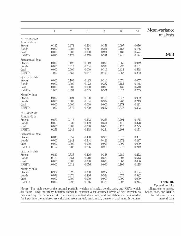
Mean-varianceanalysis
963
Table III.Optimal porfolio
allocations to stocks,bonds, cash, and REITs
for different returninterval data
1 2 3 5 8 10
A. 1972-2002Annual dataStocks 0.117 0.271 0.224 0.158 0.097 0.076Bonds 0.000 0.006 0.217 0.261 0.182 0.156Cash 0.000 0.000 0.000 0.201 0.480 0.574EREITs 0.883 0.723 0.559 0.381 0.241 0.194
Semiannual dataStocks 0.000 0.128 0.119 0.099 0.061 0.049Bonds 0.000 0.015 0.234 0.334 0.220 0.181Cash 0.000 0.000 0.000 0.113 0.432 0.538EREITs 1.000 0.857 0.647 0.453 0.287 0.232
Quarterly dataStocks 0.000 0.106 0.123 0.113 0.071 0.057Bonds 0.000 0.000 0.172 0.287 0.182 0.148Cash 0.000 0.000 0.000 0.099 0.430 0.540EREITs 1.000 0.894 0.705 0.501 0.317 0.255
Monthly dataStocks 0.000 0.121 0.138 0.112 0.077 0.062Bonds 0.000 0.000 0.134 0.332 0.267 0.213Cash 0.000 0.000 0.000 0.000 0.278 0.421EREITs 1.000 0.879 0.729 0.557 0.378 0.303
B. 1988-2002Annual dataStocks 0.671 0.418 0.333 0.266 0.204 0.155Bonds 0.069 0.339 0.429 0.501 0.471 0.378Cash 0.000 0.000 0.000 0.000 0.117 0.295EREITs 0.259 0.243 0.238 0.234 0.208 0.171
Semiannual dataStocks 0.843 0.557 0.450 0.365 0.317 0.301Bonds 0.000 0.241 0.344 0.426 0.472 0.487Cash 0.000 0.000 0.000 0.000 0.000 0.000EREITs 0.157 0.202 0.206 0.210 0.212 0.212
Quarterly dataStocks 0.811 0.535 0.426 0.338 0.289 0.272Bonds 0.189 0.451 0.518 0.572 0.603 0.613Cash 0.000 0.000 0.000 0.000 0.000 0.000EREITs 0.000 0.014 0.056 0.090 0.109 0.115
Monthly dataStocks 0.922 0.526 0.388 0.277 0.215 0.194Bonds 0.078 0.376 0.466 0.538 0.579 0.592Cash 0.000 0.000 0.000 0.000 0.000 0.000EREITs 0.000 0.098 0.146 0.185 0.207 0.214
Notes: The table reports the optimal portfolio weights of stocks, bonds, cash, and REITs whichare found using the utility function shown in equation 3 for assumed levels of risk aversion asmeasured by the parameter A. The means, standard deviations, and correlation matrices neededfor input into the analyses are calculated from annual, semiannual, quarterly, and monthly returns

MF32,12
964
more in many cases. The comparisons are most striking for more aggressive investorswith A equal to 3 or less. If the more recent history of EREITs is, in fact, moreindicative of their true nature, then using the full historical dataset could bias anyresults obtained.
Using monthly and quarterly returns instead of annual returns also has a notableimpact on optimal portfolio allocations. With the full dataset and A= 3, optimalallocations to EREITs range from 55.9 per cent with annual data to 72.9 per cent withmonthly data. For our most conservative investor with A=10, suggested allocations toEREITs range from 19.4 per cent to 30.3 per cent depending on the return interval used.The general pattern of the recommended portfolio weights is the shorter the returninterval used, the higher the optimal allocation to EREITs.
The differences due to the return intervals employed are even more pronounced usingthe more recent data as shown in panel B. While there are only minor differences in theoptimal portfolio recommendations obtained using annual and semiannual data, thedifferences are quite notable when comparing optimal portfolio weights based on annualand quarterly returns. With A=2, the recommended portfolio weights for EREITs are24.3 per cent and 1.4 per cent for annual and quarterly return intervals, respectively. Formore aggressive investors with A=8, optimal portfolio weights for EREITs are 20.8 percent with the annual data and just 10.9 per cent with quarterly data. One thought might bethat since the annual results are based on only 15 observations, there may not be sufficientdata points on which to draw conclusions. Comparing the optimal portfolio allocationsbased on quarterly returns (60 observations) vs those based on monthly returns (180observations) also reveals widely varying recommendations regarding EREITs. Exceptfor the case of A=1, all of the optimal portfolio allocations to EREITs using quarterlyinputs are 47 per cent or more less than those derivedwith monthly inputs.
Part of the divergence in the estimates of optimal portfolio weights shown in Table IIIis attributable to the annualized standard deviation figures and part is due to thedifferences in the correlation matrices obtained from the various return intervals used.The differences between the annual and annualized return figures are trivial. To removeany systematic bias associated with the annualized standard deviation calculations, weredid Table III using the mean and standard deviation figures from the annual returns. Inother words, the annual mean and standard deviation figures are used as mean-varianceinputs along with correlation matrices based on annual, semiannual, quarterly, andmonthly returns. The results of this work are shown in Table IV. For the full dataset,shown in panel A, the optimal allocations to EREITs are now comparable regardless ofthe estimation interval used. Presumably, in this case, the bulk of the differences betweenthem were associated with the annualized standard deviation calculations. For the morerecent dataset, shown in panel B, the changes do not provide a resolution. Results withannual and semiannual correlation matrices are still comparable, but the comparisonsbreak down with monthly and quarterly correlation matrices. Allocations to EREITs areconsiderably higher when using monthly correlation data as compared to quarterly data.
An examination of the correlation matrices shown in panel B of Table II reveals thefactors driving the divergences. Using monthly and quarterly returns, the stocks-EREITs correlation coefficients are quite comparable at 0.363 and 0.396, respectively.These figures are both more than double the correlations based on semiannual (0.148)and annual (0.165) returns. These relatively high monthly and quarterly correlationcoefficients make EREITs appear less attractive relative to stocks and bonds. Thedifference between the monthly and quarterly recommendations is likely to be drivenby the stocks-bonds correlation. On a monthly basis, the stocks-bonds correlation

Mean-varianceanalysis
965
Table IV.Optimal portfolio
allocations to stocks,bonds, cash, and REITsusing annual means and
standard deviations,with correlation matrices
based on annual,semiannual, quarterly,and monthly returns
1 2 3 5 8 10
A. 1972-2002Annual correlation matrixStocks 0.117 0.271 0.224 0.158 0.097 0.076Bonds 0.000 0.006 0.217 0.261 0.182 0.156Cash 0.000 0.000 0.000 0.201 0.480 0.574EREITs 0.883 0.723 0.559 0.381 0.241 0.194
Semiannual correlation matrixStocks 0.000 0.151 0.139 0.101 0.063 0.051Bonds 0.000 0.093 0.282 0.285 0.195 0.166Cash 0.000 0.000 0.000 0.227 0.493 0.582EREITs 1.000 0.756 0.579 0.387 0.248 0.202
Quarterly correlation matrixStocks 0.000 0.155 0.155 0.119 0.078 0.064Bonds 0.000 0.090 0.279 0.276 0.186 0.156Cash 0.000 0.000 0.000 0.233 0.497 0.585EREITs 1.000 0.755 0.565 0.372 0.239 0.195
Monthly correlation matrixStocks 0.058 0.189 0.160 0.120 0.078 0.064Bonds 0.000 0.101 0.280 0.312 0.205 0.170Cash 0.000 0.000 0.000 0.171 0.460 0.556EREITs 0.942 0.710 0.559 0.396 0.257 0.211
B. 1988-2002Annual correlation matrixStocks 0.671 0.418 0.333 0.266 0.204 0.155Bonds 0.069 0.339 0.429 0.501 0.471 0.378Cash 0.000 0.000 0.000 0.000 0.117 0.295EREITs 0.259 0.243 0.238 0.234 0.208 0.171
Semiannual correlation matrixStocks 0.650 0.406 0.325 0.260 0.216 0.166Bonds 0.109 0.349 0.429 0.493 0.506 0.407Cash 0.000 0.000 0.000 0.000 0.039 0.231EREITs 0.241 0.245 0.246 0.247 0.239 0.196
Quarterly correlation matrixStocks 0.670 0.444 0.365 0.301 0.265 0.218Bonds 0.330 0.488 0.535 0.573 0.594 0.502Cash 0.000 0.000 0.000 0.000 0.000 0.156EREITs 0.000 0.068 0.100 0.126 0.141 0.124
Monthly correlation matrixStocks 0.667 0.400 0.310 0.239 0.186 0.147Bonds 0.240 0.436 0.501 0.553 0.526 0.423Cash 0.000 0.000 0.000 0.000 0.089 0.266EREITs 0.093 0.165 0.189 0.208 0.199 0.163
Notes: The table reports the optimal portfolio weights of stocks, bonds, cash, and REITs whichare found using the utility function shown in equation 3 for assumed levels of risk aversion asmeasured by the parameter A. In all cases, the means and standard deviations are based onannual returns. The correlation matrices needed for input into the analyses are calculated fromannual, semiannual, quarterly, and monthly returns

MF32,12
966
coefficient is 0.134 compared to �0.083 on a quarterly basis. Obviously a lowercorrelation provides more diversification benefits, and thus, assets with a lowercorrelation become more attractive. Rather than EREITs being particularly lessdesirable in the quarterly case, it is just that stocks and bonds are more desirable.
ConclusionsMany researchers arbitrarily pick different sample periods or return intervals indetermining means, standard deviations, and correlation coefficients of asset returns tobe used in their analyses. If the estimation period and return interval used do not affectthe outcomes of the studies, then this would not be a problem. Our study with a mixed-asset portfolio including EREITs, however, suggests that both the estimation periodand the return interval employed can severely impact optimal portfoliorecommendations in mean-variance analysis.
We believe that researchers should carefully consider and justify the estimationperiod used. If, as is often suggested for REITs, more recent data is more relevant dueto the changing nature of the particular environment, then this argument should besupported and employed. Our mean-variance analysis demonstrates the importance ofthe estimation period used. With mean-variance input data from our full sample periodof 1972-2002 compared to just the more recent 1988-2002 data, recommendationsregarding EREITs changed considerably. For the full period, EREITs dominate stockswith a higher return and lower risk, and this is not the case for the more current data.
The return interval (annual, semiannual, quarterly, or monthly) used for thecalculation of mean-variance inputs also plays an important role in portfolio decisions.Decisions based on either annual or semi-annual data are generally comparable in thecase of EREITs, but results using commonly employed quarterly or monthly returnintervals diverge dramatically. Optimal portfolio recommendations based on annualand quarterly inputs varied the most, but recommendations for aggressive investorsbased on either annual or monthly data also varied considerably.
While we point out differences associated with employing various estimationintervals, we are comfortable making only limited statements as to whether oneestimation interval is better than another. In the case of standard deviations,annualized figures based on semiannual, quarterly, and monthly standard deviationssystematically understate the true annual volatility. If the desired holding period is ayear, then we believe the annual return and standard deviation figures should be used.The standard deviation based on monthly returns would be appropriate if the desiredholding period was a month. As to whether or not correlation coefficients based onmonthly and quarterly returns are applicable to annual holding periods, we suggestthat further research is necessary. Our results, though, show marked differences in thecorrelation matrices based on the return intervals employed. It may be that usingmonthly or quarterly returns provides additional observations of the true nature of therelationship between asset returns, but it could also be that short-term observationsare really not applicable to longer periods.
References
Bajtelsmit, V.L. and Worzala, E.M. (1995), ‘‘Real estate allocations in pension fund portfolios’’,Journal of Real Estate Portfolio Management, Vol. 1, pp. 25-38.
Chang, W.C. and Weiss, D.E. (1991), ‘‘An examination of the time series properties of beta in themarket model’’, Journal of the American Statistical Association, Vol. 86, pp. 883-90.

Mean-varianceanalysis
967
Clayton, J. and MacKinnon, G. (2001), ‘‘The time varying nature of the link between REIT, realestate and financial asset returns’’, Journal of Real Estate Portfolio Management, Vol. 7No. 1, pp. 43-54.
Corgel, J.B., McIntosh, W. and Ott, S.H. (1995), ‘‘Real estate investment trusts: a review of thefinancial economics literature’’, Journal of Real Estate Literature, Vol. 3, pp. 13-43.
Dopfel, F.E. (2003), ‘‘Asset allocation in a lower stock-bond correlation environment’’, Journal ofPortfolio Management, Vol. 30, pp. 25-38.
Ennis, R.M. and Burik, P. (1991), ‘‘Pension fund real estate investment under a simple equilibriumpricing model’’, Financial Analysts Journal, Vol. 47, pp. 20-30.
Firstinberg, P., Ross, S. and Zisler, R. (1988), ‘‘Real estate: the whole story’’, Journal of PortfolioManagement, Vol. 14 No. 3, pp. 22-34.
Fogler, H.R. (1984), ‘‘20% in real estate: can theory justify it?’’, Journal of Portfolio Management,Vol. 7, pp. 6-13.
Giliberto, S.M. (1992), ‘‘The allocation of real estate to future mixed-asset institutional portfolios’’,Journal of Real Estate Research, Vol. 7 No. 4, pp. 423-32.
Giliberto, S.M. (2003), ‘‘Assessing real estate volatility’’, Journal of Portfolio Management, Vol. 31No. 4 Summer 2005, September 2005, Special Real Estate Issue, pp. 122-8.
Goodman, J. (2003), ‘‘Homeownership and investment in real estate stocks’’, Journal of Real EstatePortfolio Management, Vol. 9 No. 2, pp. 93-105.
Groenewold, N. and Fraser, P. (2000), ‘‘Calculating beta: how well does the ‘five-year rule ofthumb’ do?’’, Journal of Business Finance and Accounting, Vol. 27 No. 7, pp. 953-81.
Gyourko, J. and Keim, D.B. (1993), ‘‘Risk and return in real estate: evidence from a real estatestock index’’, Financial Analysts Journal, Vol. 49 No. 5, pp. 39-46.
Hawawini, G.A. and Vora, A. (1981), ‘‘The capital asset pricing model and the investment horizon:comment’’,The Review of Economics and Statistics, Vol. 63, pp. 633-6.
Hawawini, G.A. and Vora, A. (1982), ‘‘Investment horizon, diversification, and the efficiency ofalternative beta forecasts’’,The Journal of Financial Research, Vol. 5 No. 1, pp. 1-15.
Hudson-Wilson, S. (2001), ‘‘Why real estate?’’, Journal of Portfolio Management, Vol. 27, pp. 20-32.
Kallberg, J.G., Liu, C.H. and Greig, W.D. (1996), ‘‘The role of real estate in the portfolio allocationprocess’’, Real Estate Economics, Vol. 24, pp. 359-77.
Lamb, R.P. and Northington, K. (2001), ‘‘The root of reported betas’’, Journal of Investing, Vol. 10No. 3, pp. 50-3.
Levhari, D. and Levy, H. (1977), ‘‘The capital asset pricing model and the investment horizon’’,The Review of Economics and Statistics, Vol. 59, pp. 92-104.
Levy, H. (1984), ‘‘Measuring risk and performance over alternative investment horizons’’,Financial Analysts Journal, Vol. 40, pp. 61-8.
Levy, H., Guttman, I. and Tkatch, I. (2001), ‘‘Regression, correlation, and the time interval:additive-multiplicative framework’’,Management Science, Vol. 47 No. 8, pp. 1150-9.
Levy, H. and Schwartz, G. (1997), ‘‘Correlation and the time interval over which the variables aremeasured’’, Journal of Econometrics, Vol. 76 No. 1, pp. 341-50.
Liang, Y. (1998), ‘‘REIT style and performance’’, Journal of Real Estate Portfolio Management,Vol. 4 No. 1, pp. 69-78.
Peterson, J.D. and Hsieh, C. (1997), ‘‘Do common risk factors in the returns on stocks and bondsexplain returns on REITs?’’, Real Estate Economics, Vol. 25 No. 2, pp. 321-45.
Reilly, F.K. and Wright, D.J. (1988), ‘‘A comparison of published betas’’, Journal of PortfolioManagement, Vol. 14 No. 3, pp. 64-9.

MF32,12
968
Saniga, E.M., McInish, T.H. and Gouldey, B.K. (1981), ‘‘The effect of differencing interval lengthon beta’’,The Journal of Financial Research, Vol. 4 No. 2, pp. 129-35.
Seiler, M.J., Webb, J.R. and Myer, F.C. (1999), ‘‘Diversification issues in real estate’’, Journal of RealEstate Literature, Vol. 7, pp. 163-79.
Seiler, M.J., Webb, J.R. and Myer, F.C. (2001), ‘‘Can private real estate portfolios be rebalanced/diversified using equity REITshares?’’, Journal of Real Estate Portfolio Management, Vol. 7No. 1, pp. 25-41.
Waggle, D. and Johnson, D.T. (2003), ‘‘The impact of the single-family home on portfoliodecisions’’, Financial Services Review, Vol. 12 No. 3, pp. 201-18.
Waggle, D. and Johnson, D.T. (2004), ‘‘Home ownership and the decision to invest in REITs’’,Journal of Real Estate Portfolio Management, Vol. 10 No. 2, pp. 129-44.
Waggle, D. and Moon, G. (2005), ‘‘Expected stock returns, the stock-bond correlation, and optimalasset allocations’’, Financial Services Review, Vol. 14 No. 3, pp. 253-67.
Wainscott, C.B. (1990), ‘‘The stock-bond correlation and its implications for asset allocation’’,Financial Analysts Journal, Vol. 46, pp. 55-79.
Webb, J.R., Curcio, R.J. and Rubens, J.H. (1988), ‘‘Diversification gains from including real estatein mixed-asset portfolios’’, Decision Sciences, Vol. 19 No. 3, pp. 434-52.
Ziering, B. and McIntosh, W. (1997), ‘‘Revisiting the case for including core real estate in a mixed-asset portfolio’’, Real Estate Finance, Vol. 14, pp. 14-22.
Ziering, B., Liang, Y. and McIntosh, W. (1999), ‘‘REIT correlations with capital market indexes:separating signal from noise’’, Real Estate Finance, Vol. 15 No. 4, pp. 61-7.
Corresponding authorDougWaggle can be contacted at: [email protected]
To purchase reprints of this article please e-mail: [email protected] visit our web site for further details: www.emeraldinsight.com/reprints

The TOM effectin REITs
969
Managerial FinanceVol. 32 No. 12, 2006
pp. 969-980# Emerald Group Publishing Limited
0307-4358DOI 10.1108/03074350610710463
The turn-of-the-month effectin real estate investment
trusts (REITs)William S. Compton
Cameron School of Business, University of North Carolina at Wilmington,Wilmington, North Carolina, USA
Don T. JohnsonCollege of Business and Technology, Western Illinois University,
Macomb, Illinois, USA, and
Robert A. KunkelCollege of Business Administration, University of Wisconsin at Oshkosh,
Oshkosh, Wisconsin, USA
Abstract
Purpose – This study seeks to examine the market returns of five domestic real estate investmenttrust (REIT) indices to determine whether they exhibit a turn-of-the-month (TOM) effect.Design/methodology/approach – A test is carried out for the TOM effect by employing a batteryof parametric and non-parametric statistical tests that address the concerns of distributionalassumption violations. An OLS regression model compares the TOM returns with the rest-of-the-month (ROM) returns and an ANOVA model examines the TOM period while controlling for monthlyseasonalities. A non-parametric t-test examines whether the TOM returns are greater than the ROMreturns and a Wilcoxon signed rank test examines the matched-pairs of TOM and ROM returns.Findings – A TOM effect in all five domestic REIT indices is found: real estate 50 REIT, all-REIT,equity REIT, hybrid REIT, and mortgage REIT. More specifically, the six-day TOM period, onaverage, accounts for over 100 per cent of the monthly return for the three non-mortgage REITs,while the ROM period generates a negative return. Additionally, the TOM returns are greater thanthe ROM returns in 75 per cent of the months.Research limitations/implications – The data are limited to five-years of daily returns and fivedifferent indices. Thus, the results could be biased on the selected time period.Practical implications – These results are important to REIT portfolio managers and investors.Domestic REIT markets experience a TOM effect from which investors and portfolio managers canbenefit.Orginality/value – The daily returns of all five major domestic REIT indices are examined. Dataare evaluated which include daily returns after the passage of the REIT Modernization Act of 1999that resulted in numerous changes for REITs. Whether the TOM effect can be detected with bothparametric and non-parametric tests is examined.
Keywords Real estate, Investment funds, Calendar events
Paper type Research paper
IntroductionOver the years researchers have analyzed the stock markets and identified manycalendar anomalies including the turn-of-the-month (TOM) effect[1]. Since then,researchers have found the TOM effect not only in domestic stock returns, but alsoin international stocks and domestic bonds. Several studies show that financialmarkets respond efficiently to these market anomalies by trading them out ofexistence (Agrawal and Tandon, 1994; Chow et al., 1997; Fortune, 1998; Jordan andJordan, 1991; Kamara, 1997; Riepe, 1998). Other research concludes these marketanomalies are confined to specific periods or are driven by a few outliers in the data.
The current issue and full text archive of this journal is available atwww.emeraldinsight.com/0307-4358.htm

MF32,12
970
Some of these studies suggest that market anomalies may simply be artifacts ofextensive data mining while other studies question the test methodologies sometimesused to confirm market anomalies, given the violations of OLS assumptions that havebeen identified in return distributions (Alford and Guffey, 1996; Connolly, 1989; Lindleyand Liano, 1997; Pearce, 1996; Singleton and Wingender, 1994; Sullivan et al., 2001;Kunkel et al., 2003).
One way to response to these criticisms is to test new data with more robustmethodologies. For example, if the TOM effect can be shown to exist not only in thedomestic stock market, but also in the international stock markets and bond markets,then there is solid support for a TOM effect. Additionally, if tests more robust toviolations of the OLS assumptions can identify a TOM effect in the market, then thereis even stronger support for a TOM effect. In this study we examine the daily returns offive real estate investment trust (REIT) indices to determine whether there is a TOMeffect or if investors have traded it out of existence. Using robust parametric and non-parametric tests, we find a strong TOM effect in all five indices. Additionally, we findthe TOM effect is independent of the January effect and is not driven by outlier returnsin a few months. More specifically, we find the six-day TOM period generates, onaverage, over 100 per cent of the monthly return for the three non-mortgage REITindices which means the rest-of-the-month (ROM) period is generating a negativereturn[2]. Additionally, we find the TOM returns are greater than the ROM period inalmost 75 per cent of the months.
Literature reviewAriel (1987) was the first to identify the TOM effect in stock returns. He evaluates thedaily returns over the years 1963 to 1981 for an equal-weighted (EW) stock index andvalue-weighted (VW) stock index. Ariel defines the first half of the month to include thelast trading day of the previous month and the first eight trading days of the month. Hefinds the first half of the month return is significantly greater than the last half of themonth return. More specifically, Ariel finds the 19 year cumulative returns for the firsthalf of the month to be 2552 per cent and 565 per cent on the EWand VW stock indices,respectively, while the last half of the month cumulative returns are negative for boththe EW and VW stock indices. Furthermore, Ariel finds an exceptionally strong TOMperiod in the last trading day and first four trading days of the month. Additionally, hefinds the TOM effect cannot be explained by the January effect and small-firm effect.
Lakonishok and Smidt (1988) use 90 years of daily stock returns from 1897 to 1987to examine several calendar effects including the TOM effect. They analyze the eightdays around the turn of the month and find a strong TOM effect. More specifically,they find the 0.473 per cent average four-day TOM return to be significantly greaterthan the 0.016 per cent average four-day return. They also find that over 56 per cent ofthe TOM returns are positive compared to less than 52 per cent for the average day.
The search for a TOM effect has expanded to include the domestic bond marketsand the international stock markets. Jordan and Jordan (1991) examine daily bondreturns over the years 1963 to 1986 for the Dow Jones Composite Bond Average whichis a long-term corporate bond index and find the TOM return to be 0.62 basis pointscompared to a negative return (�0.38 basis points) for the ROM return. However, thedifference is not significant at the ten per cent level. Cadsby and Ratner (1992) examinedaily stock returns in ten countries to determine if a TOM effect exists and find a TOMeffect in the stock returns of six countries: Australia, Canada, Germany, Switzerland,the United Kingdom, and the United States. However, they find no TOM effect in

The TOM effectin REITs
971
France, Hong Kong, Italy, or Japan. They also conclude the TOM effect is independentof the turn-of-the-year effect and not unique to the United States stock market. Kunkelet al. (2003) examine daily stock returns in 19 countries with standard regressionmodel, a general linear model, and a Wilcoxon signed rank (WSR) nonparametric test.They find a TOM effect in 16 of the 19 countries.
Several studies have analyzed what economic forces might be driving the TOMeffect while others have illustrated how investors can exploit the TOM effect.Lakonishok and Smidt (1988) conclude the TOM effect may be a liquidity effect that isdriven by pension fund managers buying and selling at the TOM. Ogden (1990) findsevidence that the liquidity effect is driving the TOM effect and concludes the‘‘standardization of payments system’’ in the United States is responsible for this TOMeffect. Cash receipts at the TOM include wages, retirement contributions, rent, interestand principal payments, and dividends. Much of these funds are quickly reinvested inthe stock market which results in a surge in stock returns at the TOM. Henzel andZiemba (1996) and Kunkel and Compton (1998) illustrate how the TOM effect can beexploited by institutional investors and individual investors, respectively. Both studiesuse a switching strategy where funds are invested in an equity portfolio during theTOM and invested in a interest bearing cash account during the ROM. The switchingstrategy not only generates a higher return, but also has lower return volatility.
Several papers have looked at various market anomalies in REIT returns. Colwelland Park (1990) examine daily returns over 1964 to 1986 for an equity REIT portfolioand a mortgage REIT portfolio. While they find a January effect in a portfolio of smallREITs, they find the January effect disappears in a portfolio of large REITs. They alsofind January returns for the mortgage REIT portfolio are greater than those for theequity REIT portfolio. McIntosh et al. (1991) examine daily returns over 1974 to 1988for three REIT portfolios and find a small-firm effect. Liu and Mei (1992) also examinea REIT portfolio using returns from 1971 to 1989 and find a strong January effect.Friday and Peterson (1997) examine the monthly returns over 1973 to 1993 for equity,mortgage, and hybrid REITs. They find a January effect for all sizes andclassifications. They also conclude the January effect is associated with the tax-lossselling effect.
Redman et al. (1997) examine the daily returns over 1986 to 1993 for a portfolio ofREITs and find a January effect, a TOM effect, a day-of-the-week effect, and a pre-holiday effect. To test for the TOM effect, they use a standard regression model andKruskal-Wallis test. They find the TOM return is significantly greater than zero whilethe ROM return is not significantly different from zero. Friday and Higgins (2000)examine the daily returns over 1970 to 1995 for REITs and find a day-of-the-weekeffect. They also find autocorrelated returns from Friday to Monday in equity REITs,but not for mortgage REITs. Connors et al. (2002) also evaluate REITs for seasonalpatterns by examining their daily returns over 1994 to 1999. They examine severalREIT portfolios with standard regression models and find a TOM effect and holidayeffect, but find no January effect or Monday effect.
In this study we update previous research on REITs in several ways. First, weexamine the daily returns of all five major domestic REIT indices: real estate 50, allREITs, equity REITs, hybrid REITs, and mortgage REITs. Second, we evaluate recentdata which includes daily returns after the passage of the REIT Modernization Act of1999 that resulted in numerous changes for REITs. For example, REITs could now ownup to 100 per cent of the stock of certain taxable REITsubsidiaries and the act lowered theminimum distribution requirement from 95 per cent to 90 per cent. Lastly, we examine

MF32,12
972
whether the TOM effect can be detected with both parametric and non-parametrictests. Thus, we address concerns levied by Connolly (1989), Lindley and Liano (1997),Sullivan et al. (2001) and others who revealed potential problems with standardparametric tests.
DataThe REIT industry was created in 1960 by Congress to give investors the ability toinvest in large-scale commercial properties. A REIT is a firm that owns (and oftenoperates) income producing real estate and distributes at least 90 per cent of its taxableincome to the shareholders. The REIT industry has recently experienced rapid growthwith its market capitalization growing from $8.7 billion in 1990 to $224 billion in 2003.Investors can purchase REITs that are traded on the New York Stock Exchange(NYSE), the American Stock Exchange (AMEX), and the Nasdaq Stock Market. In 2003REITs were included in various S&P indices with the S&P 500 Index, the S&P 400Mid-Cap Index, and the S&P 600 Small-Cap Index containing six, seven, and eightREITs, respectively. The commercial real estate industry continues to play a vital rolein the US economy and in 2002, it accounted for 7.2 per cent of the GDP.
In this study, we analyze daily returns of five REIT indices: real estate 50 REIT, allREIT, equity REIT, hybrid REIT, and mortgage REIT. The real estate 50 indexcontains 50 REITs that represent the most widely held REITs. The index was started inJanuary 2000 with 100 REITs (public equity 100) and was reduced to 50 REITs startingin January 2002. The All REIT index is the most comprehensive index and includesall tax-qualified REITs that trade on the NYSE, the AMEX, or the Nasdaq NationalMarket List. As of year-end 2003, the all REIT index contained 171 REITs with amarket capitalization of $224 billion. The 171 REITs invest in all nine differentproperty sectors: industrial/office, retail, residential, diversified, lodging/resorts, selfstorage, health care, specialty, and mortgage. See Figure 1 for a breakdown of theproperty sectors. The equity REIT index includes REITs that own and operate incomeproducing real estate while the Mortgage REIT index includes REITs that lend money
Industrial/Office26%
Retail26%
Residential15%
Diversified8%
Lodging/Resorts4%
Self Storage3%
Health Care6%
Specialty5%
Mortgage7%
Figure 1.REIT sectors and per centof market capitalization($241 billion as of January31, 2004)
The TOM effectin REITs
973
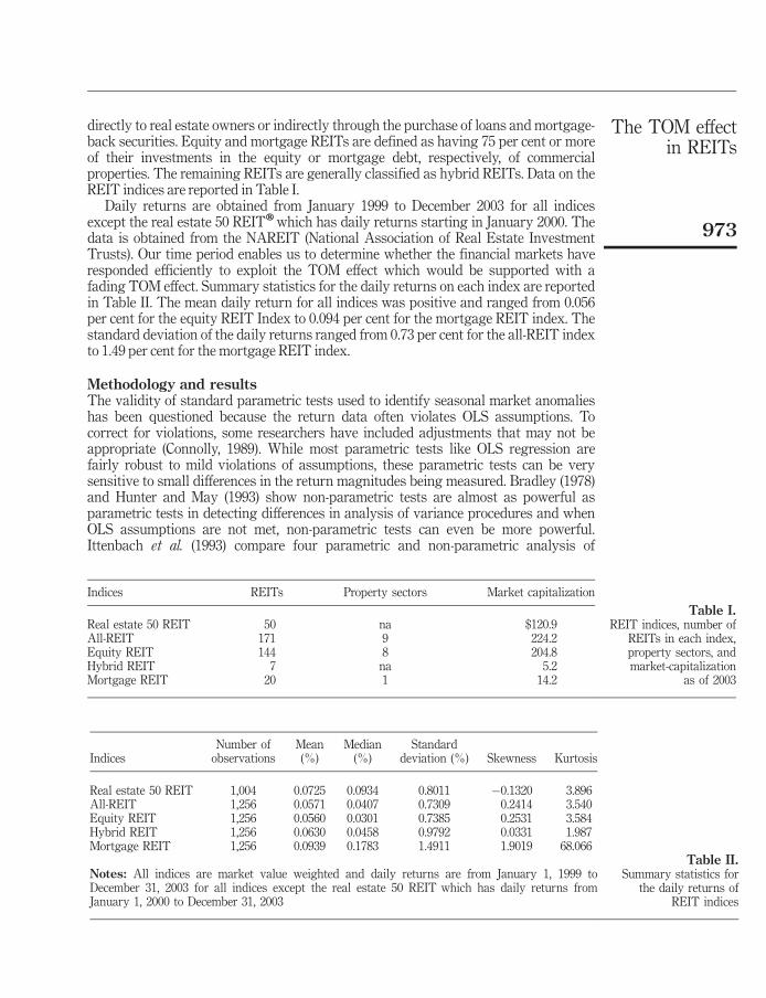
directly to real estate owners or indirectly through the purchase of loans and mortgage-back securities. Equity and mortgage REITs are defined as having 75 per cent or moreof their investments in the equity or mortgage debt, respectively, of commercialproperties. The remaining REITs are generally classified as hybrid REITs. Data on theREIT indices are reported in Table I.
Daily returns are obtained from January 1999 to December 2003 for all indicesexcept the real estate 50 REIT�which has daily returns starting in January 2000. Thedata is obtained from the NAREIT (National Association of Real Estate InvestmentTrusts). Our time period enables us to determine whether the financial markets haveresponded efficiently to exploit the TOM effect which would be supported with afading TOM effect. Summary statistics for the daily returns on each index are reportedin Table II. The mean daily return for all indices was positive and ranged from 0.056per cent for the equity REIT Index to 0.094 per cent for the mortgage REIT index. Thestandard deviation of the daily returns ranged from 0.73 per cent for the all-REIT indexto 1.49 per cent for the mortgage REIT index.
Methodology and resultsThe validity of standard parametric tests used to identify seasonal market anomalieshas been questioned because the return data often violates OLS assumptions. Tocorrect for violations, some researchers have included adjustments that may not beappropriate (Connolly, 1989). While most parametric tests like OLS regression arefairly robust to mild violations of assumptions, these parametric tests can be verysensitive to small differences in the return magnitudes being measured. Bradley (1978)and Hunter and May (1993) show non-parametric tests are almost as powerful asparametric tests in detecting differences in analysis of variance procedures and whenOLS assumptions are not met, non-parametric tests can even be more powerful.Ittenbach et al. (1993) compare four parametric and non-parametric analysis of
Table II.Summary statistics for
the daily returns ofREIT indices
IndicesNumber ofobservations
Mean(%)
Median(%)
Standarddeviation (%) Skewness Kurtosis
Real estate 50 REIT 1,004 0.0725 0.0934 0.8011 �0.1320 3.896All-REIT 1,256 0.0571 0.0407 0.7309 0.2414 3.540Equity REIT 1,256 0.0560 0.0301 0.7385 0.2531 3.584Hybrid REIT 1,256 0.0630 0.0458 0.9792 0.0331 1.987Mortgage REIT 1,256 0.0939 0.1783 1.4911 1.9019 68.066
Notes: All indices are market value weighted and daily returns are from January 1, 1999 toDecember 31, 2003 for all indices except the real estate 50 REIT which has daily returns fromJanuary 1, 2000 to December 31, 2003
Table I.REIT indices, number of
REITs in each index,property sectors, andmarket-capitalization
as of 2003
Indices REITs Property sectors Market capitalization
Real estate 50 REIT 50 na $120.9All-REIT 171 9 224.2Equity REIT 144 8 204.8Hybrid REIT 7 na 5.2Mortgage REIT 20 1 14.2

MF32,12
974
variance procedures and find the patterns of significance and statistical power to bealmost identical in three of the four approaches. Additionally, they find the non-parametric multivariate analysis of variance procedure showed a slight advantageover the other techniques. Non-parametric tests have been applied in anomaly studies,including Gultekin and Gultekin (1983), Agrawal and Tandon (1994), Alford andGuffey (1996), Ko (1998) and Kunkel et al. (2003).
When the data in Table II is examined, we find excess kurtosis and positiveskewness in the returns of four of the five REIT indices. We then test for normalityusing the Kolmogorov-Smirnov and Bowman-Shelton tests. The Kolmogorov-Smirnovtest compares the observed cumulative return distribution of the raw return data to ahypothesized cumulative distribution while the Bowman-Shelton test examines thedegree of skewness and kurtosis in the return distributions. The normal distributionassumption is rejected by both tests at the one per cent level for all REIT indices. Toaddress concerns of non-normal distributions, we use both parametric and non-parametric tests to analyze the returns of the REIT indices.
Day-of-the-month seasonalityTo examine the day-of-the-month seasonality, we test the 18 trading days around theTOM with the following OLS regression to determine if any of the mean daily returnsare significantly different from zero:
Rt ¼ ��9D�9;t þ ��8D�8;t þ � � � þ �8D8;t þ �9D9;t þ "t ð1Þ
where Rt is the return on day t; Di,t are binary dummy variables for the first and lastnine trading days of each month where D�9,t corresponds to trading day �9, D�8,t
corresponds to trading day �8, continuing through D9,t which corresponds to tradingday +9. The coefficients, ��9 to �9, represent the mean returns for the 18 trading days,and "t is the error term. While we focus on the 18 trading days surrounding the TOM,none of the other days outside that range, which range from zero to five days in anyparticular month, changed our results.
The regression results are reported in Table III and show that most significantpositive returns cluster around the TOM period, trading days �4 through +2. Over thissix-day TOM period, all indices have at least one return that is positive and significantlydifferent from zero and most indices have two to five returns that are positive andsignificantly different from zero. The table’s last column to the right shows the F-testresult which indicates there is a day-of-the-month effect for each REIT index. We reportgeneral statistics for the six-day TOM period and the 12-day ROMperiod in Table IV.
To test for a TOM effect, we use four parametric and non-parametric tests. The firsttest is a parametric OLS regression of returns onto a dummy variable for the TOMperiod. The second test is a parametric three-way analysis of variance (ANOVA) thattests the TOM period while controlling for the interaction effects of months and years.The third test is a non-parametric t-test to determine if the TOM return is greater thanthe ROM period in most months. The fourth test is a non-parametric WSR test thatexamines paired difference and controls for a January effect (or monthly effect).
OLS regression modelThe first parametric test used to identify a TOM effect is the following OLS regressionthat compares the TOM returns to the ROM returns:
Rt ¼ �þ �DTOM þ "t ð2Þ

The TOM effectin REITs
975
Table III.Mean percentage returns
for the trading daysof the month on
REIT indices
Indices
�6
�5
�4
�3
�2
�1
12
34
56
F-test(p-value)
Realestate
50REIT
A�0.147
0.143
0.215*
0.394*
0.201*
0.127
0.279*
0.218*
0.062
0.103
�0.043
�0.108
2.18
(0.0032)
All-REIT
B�0.119
0.088
0.171*
0.308*
0.132
0.257*
0.219*
0.152*
0.049
0.048
�0.050
�0.052
2.23
(0.0023)
EquityREIT
B�0.126
0.077
0.160*
0.322*
0.129
0.229*
0.231*
0.166*
0.051
0.046
�0.063
�0.057
2.20
(0.0027)
HybridREIT
B�0.159
0.216*
0.179
0.020
0.172
0.529*
0.157
0.030
�0.091
0.112
0.187
�0.197
2.35
(0.0012)
MortgageREIT
B0.110
0.318*
0.419*
0.167
0.165
0.880*
�0.106
�0.138
0.027
0.051
0.064
0.095
1.10
(0.0046)
Notes:*Significantat
the10
per
centlevel
foratw
o-tailed
t-test
that
thereturn
isdifferentfrom
zero.Regardingreturnson
tradingdays(�
9,�8,
�7,
+7,
+8,
+9),thereis
only
onetradingday
whichexperiencesapositivereturn
that
issignificantlydifferentfrom
zero.That
return
ison
tradingday
+9
oftheHybridREIT.Regardingtheother
REITs,noneof
theirreturnson
tradingdays�9,
�8,
�7,
+7,
+8,
+9aresignificantlydifferentfrom
zero

MF32,12
976
where Rt is the return on day t; � is the intercept representing the mean return for theROM period, DTOM is a binary dummy variable for the TOM period, the coefficients �represents the difference between the mean TOM return and the mean ROM return,and "t is the error term.
The F-test results are reported in Table V and show that five indices have positiveTOM returns. Furthermore, the results show the ROM return for the indices are notsignificantly different from zero. The F-statistic for each regression allows us to rejectthe null hypothesis of equality of mean returns between the TOM period and ROMperiod for all five indices. Thus, our first test finds a TOM effect in the five indices.
Next we evaluate whether a January effect could explain the high TOM returns.While studies on the January effect show stock returns are significantly higher inJanuary than the rest of the year, many studies report these higher returns aregenerated in the first few days of January. However, some studies show the TOM effectis not driven by the January effect ( Jordan and Jordan, 1991; Pettengill and Jordan,1988; Boudreaux, 1995). To test if the TOM effect exists independent of any Januaryeffect, we run the regression in equation 2 without January returns. We find that all fiveindices still show a significant TOM effect.
ANOVA modelOur next test of the TOM effect is a two-way analysis of variance model that directlycontrols for possible seasonal patterns across months. Due to the unbalanced design ofthe test, we use a general linear model procedure (GLM) which is a flexible androbust technique that detects if the TOM effect found with OLS regression is a result
Table IV.Summary statistics forthe returns over theTOM and ROM periods
Indices
TOMmean(%)
TOMstandarddeviation
(%)TOM
skewnessTOM
kurtosisROM
mean (%)
ROMstandarddeviation
(%)ROM
skewnessROM
kurtosis
Real estate50 REIT 0.239 0.843 0.530 4.592 �0.009 0.768 �0.691 3.626All-REIT 0.206 0.761 0.594 4.422 �0.019 0.682 �0.357 2.566Equity REIT 0.206 0.769 0.578 4.487 �0.022 0.688 �0.358 2.445Hybrid REIT 0.181 0.942 0.146 0.713 0.010 0.956 0.111 2.430Mortgage REIT 0.231 1.771 6.745 93.361 0.062 1.251 �0.551 7.735
Table V.Tests for the TOM effect
Indices Alpha Beta F-testGLMp-value
Non-parametrict-test
WSR testp-value
Real estate 50 REIT �0.009 0.248* 18.62* 0.001 72.9* 0.001All-REIT �0.019 0.225* 24.13* 0.001 75.0* 0.001Equity REIT �0.022 0.229* 24.42* 0.001 78.3* 0.001Hybrid REIT 0.010 0.171* 7.77* 0.024 65.0** 0.009Mortgage REIT 0.062 0.169*** 3.28*** 0.096 58.3*** 0.106
Notes: The alpha, beta and F-test values are from the OLS regression model. *Significant at the1 per cent level; **significant at the 5 per cent level; ***significant at the 10 per cent level

The TOM effectin REITs
977
of the interaction of a monthly effect such as the January effect. The GLM model is asfollows:
Rt ¼X
RPeriod;t þX
RMonth;t þ "t ð3Þ
where RPeriod represents returns for the TOM and ROM periods and RMonth accountsfor any interaction effects due to a monthly effect. In Table V we report the F-testresults across periods (TOM versus ROM) and show the null hypothesis is rejected forall five REIT indices at the one per cent significance level. This supports a strong TOMeffect in all five REIT indices, even after accounting for differences across months.
Non-parametric t-testOur next test of the TOM effect is a non-parametric (or binomial) t-test to determine ifthe TOM return is greater than the ROM return in more than 50 per cent of the months.The equation for the non-parametric t-test is:
� ¼ p� 0:5
½ð0:5Þð0:5Þ=n�0:5ð4Þ
where p is the observed sample proportion, n is the sample size, and (n� 1) is thedegrees of freedom.
We find the TOM return is greater than the ROM return in over 70 per cent of themonths for the three non-mortgage REIT indices: real estate 50 REIT, all-REIT, andequity REIT. For the non-mortgage REIT indices, we find the TOM return is greaterthan the corresponding ROM return in 75 per cent of the months with a range from 73per cent for the real estate 50 REIT Index to 78 per cent for the equity REIT index. TheTOM return is greater in 65 per cent and 58 per cent of the months for the hybrid REITand mortgage REIT, respectively. In Table V we report the t-test results and find theTOM return is greater than the ROM return in more than 50 per cent of the months.Thus, the third test supports a TOM effect in all five REIT indices.
WSR testOur last test is the WSR test which is a non-parametric paired differences test.The WSR test parallels the layout of the parametric two-way ANOVA, but does notassume the data is normally distributed as does the regression and ANOVAprocedures. The WSR procedure tests the difference in medians rather than means, isbased only on the ranks of the paired differences between TOM and ROM returns, andcontrols implicitly for differences across months. This means the WSR procedure ismore robust than a regression or two-way ANOVA when the data is not normallydistributed or there is a violation of homogeneous variance in the data because theWSR test considers only the ranks of return differences while ignoring differences inreturn magnitude.
The WSR test consists of sorting the absolute values of the differences from smallestto largest, assigning ranks to the absolute values, and finding the sum of the ranks of thepositive differences, which under the null hypothesis should be about the same as thesum of the ranks of the negative differences. If sum of ranks for the positive and negativedifferences are not the same, then the WSR test will be significant even if the magnitudeis small. The WSR test statistic is asymptotically distributed as a chi-squared with k� 1degrees of freedom. The WSR test results are reported in Table V and show a strongTOM effect in all the REIT indices, except the mortgage REIT index.

MF32,12
978
ConclusionWe obtain daily returns from 1999 to 2003 on five domestic REIT indices. We test forthe TOM effect by employing a battery of parametric and non-parametric statisticaltests that address the concerns of distributional assumption violations raised inprevious studies. The first test is a parametric OLS regression model that compares theTOM returns to the ROM returns. The second test is a parametric analysis of variance(ANOVA) model that examines the TOM period while controlling for monthlyseasonalities. The third test is a non-parametric t-test that examines whether the TOMreturn is greater than the ROM return in more than 50 per cent of the months. Thefourth test is a non-parametric WSR test that examines the matched-paired of TOMand ROM returns.
All four tests find a strong TOM effect in four of the five domestic REIT indices: realestate 50 REIT, all-REIT, equity REIT, and hybrid REIT. More specifically, we find thesix-day TOM period, on average, accounts for over 100 per cent of the monthly returnfor the three non-mortgage REITs while the ROM period generates a negative return.Additionally, their TOM returns are greater than the ROM return in 75 per cent of themonths. We also find the hybrid REIT index (a mix of equity and mortgage REITs)exhibits a TOM effect. However, the results for the mortgage REIT Index are mixed.While the parametric tests conclude there is a TOM effect the nonparametric WSR testdoes not find a TOM effect. In summary, it is clear the TOM effect is a phenomenonthat can be found not only in domestic stock markets, international stock markets, anddomestic bond markets, but also in domestic non-mortgage REITmarkets.
Notes
1. Calendar anomalies include: January effect (Rozeff and Kinney, 1976; Keim, 1983; Roll,1983; Reinganum, 1983), weekend effect (Cross, 1973; French, 1980; Gibbons and Hess,1981; Keim and Stambaugh, 1984); TOM effect (Ariel, 1987); holiday effect (Ariel, 1990);Friday the Thirteenth effect (Kolb and Rodriguez, 1987).
2. Our results are similar to Agrawal and Tandon (1994) and Kunkel et al. (2003) whofound in many countries that the TOM period can generate between 70 and 87 per centof the monthly return.
References
Agrawal, A. and Tandon, K. (1994), ‘‘Anomalies or illusions? Evidence from stock markets ineighteen countries’’, Journal of International Money and Finance, Vol. 12, pp. 83-106.
Alford, A. and Guffey, D. (1996), ‘‘A re-examination of international seasonalities’’, Journal ofFinancial Economics, Vol. 5, pp. 1-17.
Ariel, R. (1987), ‘‘A monthly effect in stock returns’’, Journal of Financial Economics, Vol. 18,pp. 161-74.
Ariel, R. (1990), ‘‘High stock returns before holidays’’, Journal of Finance, Vol. 45, pp. 1611-26.
Boudreaux, D. (1995), ‘‘The monthly effect in international stock markets: evidence andimplications’’, Journal of Financial and Strategic Decisions, Vol. 8, pp. 15-20.
Bradley, J. (1978), Distribution Free Statistical Tests, Prentice-Hall, Englewood Cliffs, NJ.
Cadsby, C. and Ratner, M. (1992), ‘‘Turn-of-month and pre-holiday effects on stock returns: someinternational evidence’’, Journal of Banking and Finance, Vol. 16, pp. 497-509.
Chow, E., Hsiao, P. and Solt, M. (1997), ‘‘Trading returns for the weekend effect using intradaydata’’, Journal of Business Finance and Accounting, Vol. 24, pp. 425-44.

The TOM effectin REITs
979
Colwell, P. and Park, H. (1990), ‘‘Seasonality and size effects: the case of real-estate-relatedinvestment’’, Journal of Real Estate Finance and Economics, Vol. 3, pp. 251-9.
Connolly, R. (1989), ‘‘An examination of the robustness of the weekend effect’’, Journal ofFinancial and Quantitative Analysis, Vol. 24, pp. 133-69.
Connors, D., Jackman, M., Lamb, R. and Rosenberg, S. (2002), ‘‘Calendar anomalies in the stockreturns of real estate investment trust’’, Briefings in Real Estate Finance, Vol. 6, pp. 61-71.
Cross, F. (1973), ‘‘The behavior of stock price on Fridays and Mondays’’, Financial AnalystsJournal, Vol. 29, pp. 67-9.
Fortune, P. (1998), ‘‘Weekends can be rough: revisiting the weekend effect in stock prices’’, FederalReserve Bank of Boston, working paper no. 98-6.
French, K. (1980), ‘‘Stock returns and the weekend effect’’, Journal of Financial Economics, Vol. 8,pp. 55-69.
Friday, H. and Higgins, E. (2000), ‘‘The day of the week effect in real estate investment trusts’’,Journal of Real Estate Portfolio Management, Vol. l, pp. 273-81.
Friday, H. and Peterson, D. (1997), ‘‘January return seasonality in real estate investment trusts:information vs. tax-loss selling effects’’, The Journal of Financial Research, Vol. 20,pp. 33-51.
Gibbons, M. and Hess, P. (1981), ‘‘Day of the week effects and asset returns’’, Journal of Business,Vol. 54, pp. 579-96.
Gultekin, M. and Gultekin, N. (1983), ‘‘Stock market seasonality: international evidence’’, Journalof Financial Economics, Vol. 12, pp. 469-81.
Hensel, R. and Ziemba, W. (1996), ‘‘Investment results from exploiting TOM effects’’, Journal ofPortfolio Management, Vol. 22, pp. 17-23.
Hunter, M. and May, R. (1993), ‘‘Some myths concerning parametric and nonparametric tests’’,Canadian Psychology, Vol. 34, pp. 384-9.
Ittenbach, R., Chayer, D., Bruininks, R., Thurlow, M. and Beirne-Smith, M. (1993), ‘‘Adjustment ofyoung adults with mental retardation in community settings: comparison of parametricand nonparametric statistical techniques’’, American Journal on Mental Retardation,Vol. 97, pp. 607-15.
Jordan, S. and Jordan, B. (1991), ‘‘Seasonality in daily bond returns’’, Journal of Financial andQuantitative Analysis, Vol. 26, pp. 269-85.
Kamara, A. (1997), ‘‘New evidence on the Monday seasonal in stock returns’’, Journal of Business,Vol. 70, pp. 63-84.
Keim, D. (1983), ‘‘Size-related anomalies and stock return seasonality: further empirical evidence’’,Journal of Financial Economics, Vol. 12, pp. 13-32.
Keim, D. and Stambaugh, R. (1984), ‘‘A further investigation of the weekend effect in stockreturns’’, Journal of Finance, Vol. 39, pp. 819-35.
Ko, K. (1998), ‘‘Strategic international diversification and monthly seasonality’’, Journal ofBusiness Finance and Accounting, Vol. 25, pp. 203-21.
Kolb, R. and Rodriguez, R. (1987), ‘‘Friday the thirteenth: part vii – a note’’, Journal of Finance,Vol. 43, pp. 1385-7.
Kunkel, R. and Compton, W. (1998), ‘‘A tax-free exploitation of the TOM effect: C.R.E.F’’, FinancialServices Review, Vol. 7, pp. 11-23.
Kunkel, R., Compton, W. and Beyer, S. (2003), ‘‘The turn-of-the-month effect still lives: theinternational evidence’’, International Review of Financial Analysis, Vol. 12, pp. 207-21.
Lakonishok, J. and Smidt, S. (1988), ‘‘Are seasonal anomalies real? A ninety-year perspective’’,Review of Financial Studies, Vol. 1, pp. 403-25.

MF32,12
980
Lindley, J. and Liano, K. (1997), ‘‘An evaluation of anomalies across years: significance versususefulness’’, working paper no. 97-03.
Liu, C. and Mei, J. (1992), ‘‘The predictability of returns on equity REITs and their co-movementswith other assets’’, Journal of Real Estate Finance and Economics, Vol. 5, pp. 401-18.
McIntosh, W., Liang, Y. and Tompkins, D. (1991), ‘‘An examination of the small-firm effect withinthe REIT industry’’,The Journal of Real Estate Research, Vol. 6, pp. 9-17.
Ogden, J. (1990), ‘‘Turn-of-month evaluations of liquid profits and stock returns: a commonexplanation for the monthly and January effects’’, Journal of Finance, Vol. 45, pp. 1259-72.
Pearce, D. (1996), ‘‘The robustness of calendar anomalies in daily stock returns’’, Journal ofEconomics and Finance, Vol. 20, pp. 69-80.
Pettengill, G. and Jordan, B. (1988), ‘‘A comprehensive examination of volume effects andseasonality in daily security returns’’, Journal of Financial Research, Vol. 11, pp. 57-70.
Redman, A., Manakyan, H. and Liano, K. (1997), ‘‘Real estate investment trusts and calendaranomalies’’, Journal of Real Estate Research, Vol. 14, pp. 19-27.
Reinganum, M. (1983), ‘‘The anomalous stock market behavior of small firms in January:empirical tests for tax-loss selling effects’’, Journal of Financial Economics, Vol. 12,pp. 89-104.
Riepe, M. (1998), ‘‘Is publicity killing the January effect?’’, Journal of Financial Planning, Vol. 11,pp. 64-70.
Roll, R. (1983), ‘‘Vas ist das? The turn of the year effect and the return premium of small firms’’,Journal of Portfolio Management, Vol. 9, pp. 18-28.
Rozeff, M. and Kinney, W. (1976), ‘‘Capital market seasonality: the case of stock returns’’, Journalof Financial Economics, Vol. 3, pp. 379-402.
Singleton, J. and Wingender, J. (1994), ‘‘The nonparallel weekend effect in the stock and bondmarkets’’, Journal of Financial Research, Vol. 17, pp. 531-8.
Sullivan, R., Timmermann, A. andWhite, H. (2001), ‘‘Dangers of data mining: the case of calendareffects in stock returns’’, Journal of Econometrics, Vol. 105, pp. 249-86.
Corresponding authorRobert A. Kunkel can be contacted at: [email protected]
To purchase reprints of this article please e-mail: [email protected] visit our web site for further details: www.emeraldinsight.com/reprints

REIT capitalstructure
981
Managerial FinanceVol. 32 No. 12, 2006
pp. 981-987# Emerald Group Publishing Limited
0307-4358DOI 10.1108/03074350610710472
REIT capital structure: is itmarket imposed?
K. Michael CaseyDepartment of Economics, Finance, Insurance and Risk Management,College of Business Administration, University of Central Arkansas,
Conway, Arkansas, USA, and
Glenna Sumner and James PackerHenderson State University, Arkadelphia, Arkansas, USA
Abstract
Purpose – This study sets out to focus on the identification of determinants of real estate limitedpartnership (REIT) capital structure from a market perspective.Design/methodology/approach – This study uses ordinary least squares regression to testwhether REIT capital structure is impacted by various market variables.Findings – The findings indicate that investors do appear to be attracted to specific debtcharacteristics of REITs or, simply put, REIT capital structure is influenced by market factors. REITdebt levels appear to be directly influenced by the price-to-book ratio and are inversely related to thepercentage of institutional ownership and price-to-cash flow. Forecast growth rates do not appear tosignificantly influence debt while the type of REIT (mortgage, retail, etc.) does appear to influence thelevel of debt.Research limitations/implications – Small sample size limits applicability of results, so furtherresearch with larger datasets is appropriate.Practical implications – Investors do appear to consider capital structure when purchasing REITs.REIT managers should consider this when determining whether to incur additional debt.Originality/value – The determination of various market factors linked to REIT capital structure.
Keywords Real estate, Capital structure, Market forces, Debt financing
Paper type Research paper
1. IntroductionThe concept of an optimal capital structure for business firms remains a cornerstone offinancial economics theory since the seminal works of Modigliani and Miller (1958;1963) that focused on tax benefits and other costs of debt. While many aspects of thecorporate capital structure puzzle have been filled in, many questions remain. Theemphasis in current research has shifted to nontax-driven capital structure theories asextensively surveyed by Harris and Raviv (1991). While they reviewed over 150 paperson the topic (just since the mid-1970s), that number is now in the hundreds.
One of the four identified models or categories of the determinants of capitalstructure within the nontax theories is the agency theory approach and a desire toreduce the conflicts of interest that arise among the parties to the firm. Jensen andMeckling (1976) assert that as management owns less and less of a firm’s equity,conflicts of two types arise. Conflict one is between managers and shareholders.Conflict two is between equity holders and debt holders.
The conflict between management and equity holders arises when managers ownless than 100 per cent of the equity. In that commonplace instance, managers do notreceive 100 per cent of the gain when their actions enhance firm value. Therefore,management has an incentive to consume excessive levels of perquisites such ascorporate limos, apartments, aircraft, etc. This inefficiency is naturally mitigated thelarger management’s ownership position. Increases in the portion of the firm financed
The current issue and full text archive of this journal is available atwww.emeraldinsight.com/0307-4358.htm

MF32,12
982
by debt thereby increase the manager’s equity share and somewhat mitigatesmanagement’s loss from the manager-equity holder conflict.
The second conflict arises because equity holders have some incentive to invest inless-than-optimal projects. Larger than normal returns from an investment are morelikely to be captured by equity holders than by debt holders. Additionally, bankruptcycosts can be increased if equity holders ‘‘shoot the moon’’ with risky investments anddebt holders can be penalized. Several authors have also pointed out that agency costscan be mitigated through managerial incentives in compensations plans or convertibledebt (see Brander and Poitevin (1989), Dybvig and Zender (1989), Narayanan (1987)and Haugen and Senbet (1987)).
However, a firm seeking external capital (either equity or debt) receives the scrutinyof these respective capital markets. Monitoring functions automatically take place thathelp ensure that management behaves in a manner consistent with maximizingshareholder wealth. Additionally, debt can also reduce agency costs by reducing freecash flow and forcing management to operate more efficiently to service the debt andreduce the threat of bankruptcy. Stultz (1990), Jensen (1986), and Maloney et al. (1993)all provide arguments supporting the assertion that debt can improve managerialdecision-making.
Another factor that may work to mitigate agency costs and influence capitalstructure is institutional ownership. Demsetz (1983) and Shliefer and Vishny (1986)suggest that institutional investors have natural incentives to monitor management.Agarwal and Mandelker (1990), Brickley et al. (1988) and McIntyre and Rao (1993) allreport evidence of various aspects of the firm being influenced by institutionalinvestors. Friend and Lang (1988) suggest that managers can be motivated by a higherdebt ratio demanded by at least one large non-managerial shareholder.
Chaganti and Damanpour (1991) and Grier and Zychowicz (1994) both find aninverse relationship between the level of institutional ownership and debt. Grier andZychowicz contend that aggressive monitoring of managers by institutional ownersthrough the corporate governance process may ‘‘substitute’’ for the monitoring role ofdebt. Perhaps large block shareholders have advantages in monitoring corporateactivity that individual investors do not have.
However, contrary findings are presented by Casey and Anderson (1997) whoexamine capital structure in the petroleum industry and conclude that ‘‘higher levels ofinstitutional ownership are significantly related to higher levels of debt’’. Certainly,though, their result may turn out to be industry specific.
Many studies report that industries tend to have target capital structures. Bowenet al. (1982), Bradley et al. (1984), Long and Malitz (1985), Kester (1986), and Titman andWessels (1988) all find a link between industry affiliation and capital structure. Scottand Johnson’s 1982 survey of CFOs finds that leverage determination is ‘‘benchmarked’’with industry average factors. Logically, industry capital structure could evolvebecause exogenous variables tend to impact similar firms in similar ways.
Other researchers target only one industry at a time. McCue (1992) investigateshospital capital structure and Sharpe (1995) studies Australian trading banks. Capitalstructure determinants for real estate limited partnerships (REITs) have gotten someattention.
Maris and Elayan (1990) examine the relationship between capital structure and thecost of capital in REITs from 1981 to 1987. They report a ‘‘leverage clientele effect’’ asan incentive for REITs to use debt. A study by Theis and Casey (1999) comes theclosest to a recent examination of REIT-like firms by analyzing property management

REIT capitalstructure
983
firms in the UK. Their findings indicate that debt is inversely related to percentage ofshares closely held, dividend yield and the price-to-book ratio.
REITs appear to be an ideal proxy for nontax-driven capital structure researchsince they commonly avoid corporate taxation. Additionally, in cases of being held inportfolios of pension funds, endowments, IRAs, 401Ks, etc. REITs can avoid personaltaxes for many years.
In addition to Maris and Elayan (1990), the Bradley et al. (1984) study includes asub-sample of REITs and finds that REITs are more heavily leveraged than 16 of the 25industries they studied from the 1960s and 1970s. Howe and Shilling (1988) reportpositive wealth effects from announcements of REIT debt offerings. Providing acounter argument, Jaffe (1991) examines real estate partnerships and REITs anddetermines that capital structure does not influence firm value. Hamill’s (1993) findingsagree with Howe and Shilling in terms of REIT capital structure and the relationshipwith value.
Allen’s (1995) examination of RELPs finds a negative link between growth rates andnondebt tax shields and a firm’s level of debt. However, research identifying theimportant capital structure determinants for REITs is scarce. In addition toinstitutional ownership, this study examines other market variables suggested by theliterature that might impact capital structure decisions for REITs including: price-to-book, price-to-cash flow, dividend yield, and forecast revenue growth. We also include adummy variable coded one for mortgage REITs to see if REIT type impacts capitalstructure.
The rest of the paper is organized as follows. Section II discusses the dataand methodology. Section III analyzes the findings and section IV provides someconclusions and makes recommendations.
2. Data and methodologyThe data for this study were obtained from various free online sources such as ReutersMultex Investor and Yahoo Finance. A full set of data is available for 89 REITs listedon US stock exchanges. The methodology is a linear regression model with onedependent and six independent variables. A presentation of the model follows:
DEBTj ¼ �þX
�iXij þ "
where DEBT ¼ debt to equity ratio, and Xij represents each independent variable i,for each firm j. These variables are:
GROWTH=% forecast five year growth rate in revenues;INSTIT=% institutional ownership;PBOOK=price-to-book ratio;PCASHFLOW=price-to-cash flow ratio;DIVY=% dividend yield;MORTGAGE=dummy variable coded 1 for mortgage REITs, 0 otherwise;"= an error term.
A more detailed discussion of the variables and their measurement follows. Thedependent variable, DEBT, is the percentage of long-term debt in the capital structureof each REIT for their most recent reporting period typically ending in 2003.
GROWTH is the consensus analyst forecast five-year growth rate in revenues.Firms expecting higher growth rates are assumed to also have greater needs for capital
MF32,12
984
and thus would be expected to incur additional debt. We would expect GROWTH to bepositively related to debt levels. However, Allen (1995), in his study of RELP capitalstructure, found the relationship between growth and debt to be negative.
INSTIT is the percentage of equity held by institutional owners. Grier andZychowicz (1994) find the relationship between level of institutional ownership anddebt to be negative. Their study maintains that institutional ownership may substitutefor the monitoring role of debt in the agency model. Additionally, their study concludedthat institutional owners may actually influence debt levels.
PBOOK[1], or the price-to-book ratio, is a recent market price divided by the bookvalue per share. Fama and French (1995) find that firms with higher PBOOK ratiostend to generate higher returns and are also generally growth stocks. Therefore,PBOOK could serve as an investor proxy for future growth. Growth firms may beforced into the external market for additional debt financing, particularly in the REITindustry with greater stability of cash flows.
PCASHFLOW, or the price-to-cash flow ratio, should serve as a proxy for investorinterest in a company. REITs with higher PCASHFLOW ratios could be consideredinvestor favorites. The justification for including this variable is to examine whetherinvestors are attracted to higher or lower debt REITs. The sign could, therefore, bepositive or negative.
DIVY, or dividend yield (most recent annualized dividend divided by price), isanother variable expected to proxy investor interest in the firm. Higher yields couldsignal lower levels of investor enthusiasm as a dollar of dividends received a lowermarket valuation. This variable is also included to determine whether investors areattracted to a certain REIT capital structure. This sign could also be positive ornegative.
MORTGAGE, a dummy variable for mortgage REITs, was also included due to thecash flow certainty differences between mortgage REITs and other classes. MortgageREITs are expected to carry higher levels of debt because of the predictability of cashflows.
3. Empirical resultsTable I presents the ordinary least squares regression results achieved from runningvariations of the previously specified model. All three models are significant at the 0.05level or better. However, it is obvious that model three, where a dummy variable formortgage REITs was included, is far superior to the other two models. Theexplanatory power of the model increases from 0.158 (model 1) to 0.414 with theaddition of the dummy variable MORTGAGE.
Note that the individual variables representing institutional ownership (INSTIT)and PCASHFLOW are both negative and significant in model one. However, when thedummy variable MORTGAGE is included, the model loses the significance attributedto institutional ownership. Conversely, PBook remains positive and significant in allthree models.
Also note that forecast growth rates are not significant in any model, contrary toexpectations about future growth serving as an indicator of financing needs. Dividendyield, also related to growth prospects, was also not significant in model 2.
4. ConclusionsThe finding of a significant inverse relationship between institutional ownership anddebt in model 1 partially confirms the research of Chiganti and Damanpour (1991) and

REIT capitalstructure
985
Grier and Zychowicz (1994), at least as it pertains to REITs. However, when dividendyield or mortgage REIT variables are included, institutional ownership turnsinsignificant. This finding indicates that while for most REITs institutional ownersmight prefer lower levels of debt it appears that mortgage REITs are considered to beenough lower in risk, probably due to the predictability in cash flows and theavailability of mortgage insurance, to support higher levels of debt.
The significance of the variable PCASHFLOW, and the inverse relationship, in allthree models is intriguing. As PCASHFLOW increases debt levels go down. Investorsappear to bid up the price of non-mortgage REITs relative to each dollar of cash flowdepending on debt levels. The implications are that non-mortgage REITs should optfor lower levels of debt, while mortgage REITs should take on additional debt.
The positive relationship between debt and price-to-book is also interesting. It ispossible that PBOOK is not a good proxy for investor growth expectations. However,this finding could be explained at least partially by the age of the assets. Non-mortgageREITs, in particular, could be carrying older assets that are closer to being paid for andthus investors will bid up the price relative to the book value. This discrepancybetween true market value of the assets and book value could also inflate the debt toequity ratio and create this relationship.
When considering the overall models, investors appear to gravitate towards certaincapital structures and REIT market values should reflect these preferences. Capitalstructure, at least for REITs, should be considered by managers attempting to optimizevalue and also investors looking for REITs likely to appreciate.
This area of investigation could be greatly expanded with additional data and thusis one limitation of this study. Further research could explore many other agencyfactors shown to impact capital structure in other industries.
Note
1. An anonymous reviewer suggested this variable might be correlated with GROWTH.Analysis of the correlation matrix indicates low correlation between the two growthmeasures with a coefficient of 0.251.
Table I.REIT industry OLS
regression results forthe period ending2003 T-values are
in parentheses(Dependent =Debt)
Model: Debtj ¼ B0 þX
B1Xij þ e
Variables Regression model 1 Regression model 2 Regression model 3
CONSTANT 1.507 (1.598) 1.074 (0.917) 1.093 (1.372)GROWTH 0.186 (1.415) 0.172 (1.294) 0.111 (1.000)INSTIT �1.858E-02 (�1.768)* �1.724E-02 (�1.555) �1.020E-02 (�1.136)PBOOK 1.140 (2.685)* 1.107 (2.581)* 0.929 (2.588)*P CASH FLOW �0.184 (�2.296)* �0.166 (�1.995)* �0.122 (�1.779)*DIVY 3.572E-02 (0.660)MORTGAGE 5.178 (5.291)*
F-statistic (p-value) 3.046 (0.023) 2.460 (0.042) 9.047 (0.000)
R2 0.158 0.163 0.414
Notes: *Significant at the 0.10 level or better; DEBT=debt to equity ratio; GROWTH=% forecastfive year growth rate in revenues; INSTIT=% institutional ownership; PBOOK=price-to-bookratio; P CASH FLOW=price-to-cash flow ratio; DIVY=dividend yield; MORTGAGE=dummyvariable coded 1 for mortgage REITs, 0 otherwise

MF32,12
986
References
Agarwal, A. and Mandelker, G.N. (1990), ‘‘Large shareholders and the monitoring of managers:the case of antitakeover amendments’’, Journal of Financial and Quantitative Analysis,Vol. 25, pp. 143-61.
Allen, M.T. (1995), ‘‘Capital structure determinants in real estate limited partnerships’’, TheFinancial Review, Vol. 30 No. 3, pp. 399-426.
Bowen, R., Daly, L. and Huber, C., Jr. (1982), ‘‘Evidence on the existence and determinants of inter-industry differences in leverage’’, Financial Management, Vol. 11, pp. 10-20.
Bradley, M., Jarrell, G. and Kim, E.H. (1984), ‘‘On the existence of an optimal capital structure:theory and evidence’’, Journal of Finance, Vol. 39, pp. 857-78.
Brander, J. and Poitevin, M. (1989), ‘‘Managerial compensation and the agency costs of debtfinance’’, working paper, University of British Columbia.
Brickley, J.A., Lease, R.C. and Smith, C.W., Jr. (1988), ‘‘Ownership structure and the monitoringof managers’’, Journal of Financial Economics, Vol. 20, pp. 267-91.
Casey, K.M. and Anderson, D.C. (1997), ‘‘A note on institutional ownership and capital structure:evidence from the petroleum industry’’,Oil and Gas Tax Quarterly, Vol. 45 No. 4, pp. 727-36.
Chaganti, R. and Damanpour, F. (1991), ‘‘Institutional ownership, capital structure, and firmperformance’’, Strategic Management Journal, Vol. 12, pp. 479-91.
Demsetz, H. (1983), ‘‘The structure of ownership and the theory of the firm’’, Journal of Law andEconomics, Vol. 26, pp. 375-90.
Dybvig, P. and Zender, J. (1989), ‘‘Capital structure and dividend irrelevance with asymmetricinformation’’, working paper, Yale School of Organization and Management.
Fama, E.F. and French, K.R. (1995), ‘‘Size and book-to-market factors in earnings and returns’’,Journal of Finance, Vol. 50, pp. 141-55.
Friend, I. and Lang, L. (1988), ‘‘An empirical test of the impact of management self-interest oncorporate capital structure’’, Journal of Finance, Vol. 43, pp. 271-81.
Grier, P. and Zychowicz, E.J. (1994), ‘‘Institutional investors, corporate discipline, and the role ofdebt’’, Journal of Economics and Business, Vol. 46, pp. 1-11.
Hamill, J.R. (1993), ‘‘A note on taxes and capital structure of partnerships, REITs, and relatedentities’’, Journal of Real Estate Research, Vol. 8, pp. 279-86.
Harris, M. and Raviv, A. (1991), ‘‘The theory of capital structure’’, The Journal of Finance, Vol. 46No. 1, pp. 297-355.
Haugen, R. and Senbet, L. (1987), ‘‘On the resolution of agency problems by complex financialinstruments: a reply’’, Journal of Finance, Vol. 42, pp. 1091-5.
Howe, J.S. and Shilling, J.D. (1988), ‘‘Capital structure theory and REIT security offerings’’, Journalof Finance, Vol. 43 No. 4, pp. 983-93.
Jaffe, J.F. (1991), ‘‘Taxes and the capital structure of partnerships, REITs and related entities’’,Journal of Finance, Vol. 46, pp. 401-7.
Jensen, M.C. and Meckling, W. (1976), ‘‘Theory of the firm: management behavior, agency costsand capital structure’’, Journal of Financial EconomicsVol. 3, pp. 305-60.
Jensen, M.C. (1986), ‘‘Agency costs of free cash flow, corporate finance and takeovers’’, AmericanEconomic Review, Vol. 76, pp. 323-9.
Kester, W.C. (1986), ‘‘Capital and ownership structure: the comparison of United States andJapanese manufacturing corporations’’, Financial Management, Vol. 15, pp. 5-16.
Long, M. and Malitz, E. (1985), ‘‘The investment-financing nexus: some empirical evidence’’,Midland Corporate Finance Journal, Vol. 3, pp. 53-9.

REIT capitalstructure
987
Maloney, M., McCormick, R.E. and Mitchell, M.L. (1993), ‘‘Managerial decision making andcapital structure’’, Journal of Business, Vol. 66 No. 2, pp. 189-217.
Maris, B.A. and Elayan, F.A. (1990), ‘‘Capital structure and the cost of capital for untaxed firms:the case of REITs’’,AREUEA Journal, Vol. 18 No. 1, pp. 22-39.
McCue, M.J. (1992), ‘‘Determinants of capital structure’’, Hospital and Health ServicesAdministration, Vol. 37, pp. 333-46.
McIntyre, J.E., Jr. and Rao, V.K. (1993), ‘‘The effects of institutional ownership on bank CEOcompensation’’, Journal of Business and Economic Perspectives, Vol. 19 No. 2, pp. 25-31.
Modigliani, F. and Miller, M.H. (1958), ‘‘The cost of capital, corporation finance, and the theory ofinvestment’’,American Economic Review, Vol. 53 No. 3, pp. 261-97.
Modigliani, F. and Miller, M.H. (1963), ‘‘Corporate income taxes and the cost of capital’’, AmericanEconomic Review, Vol. 53 No. 3, pp. 433-43.
Narayanan, M.P. (1987), ‘‘On the resolution of agency problems by complex financial instruments:a comment’’, Journal of Finance, Vol. 42, pp. 1083-90.
Sharpe, I.G. (1995), ‘‘Determinants of capital structure of australian trading banks’’, Asian PacificJournal of Management, Vol. 12, pp. 97-121.
Shleifer, A. and Vishny, R. (1986), ‘‘Large shareholders and corporate control’’, Journal of PoliticalEconomy, Vol. 94, pp. 461-88.
Stultz, R. (1990), ‘‘Managerial discretion and optimal financing policies’’, Journal of FinancialEconomics, Vol. 26, pp. 3-27.
Theis, J. and Casey, M. (1999), ‘‘An empirical investigation of agency relationships and capitalstructure of property management firms in the UK’’, Journal of Property Investment andFinance, Vol. 17 No. 1, pp. 27-34.
Titman, S. and Wessels, R. (1988), ‘‘The determinants of capital structure choice’’, The Journal ofFinance, Vol. 43, pp. 1-20.
Further reading
Financial Economists Roundtable (1998), Statement on Institutional Investors and CorporateGovernance, Annual meeting in July 1998, Boothbay Harbor, Maine, pp. 1-5.
Oppenheimer, P. (2000), ‘‘An investigation of current debt levels of equity REITs’’, Journal of RealEstate Portfolio Management, Vol. 6 No. 3, pp. 225-37.
Corresponding authorK. Michael Casey can be contacted at: [email protected]
To purchase reprints of this article please e-mail: [email protected] visit our web site for further details: www.emeraldinsight.com/reprints

MF32,12
988
Managerial FinanceVol. 32 No. 12, 2006pp. 988-996# Emerald Group Publishing Limited0307-4358DOI 10.1108/03074350610710481
Manager characteristics and realestate mutual fund returns,
risk and feesJames Philpot
Missouri State University, Springfield, Missouri, USA, and
Craig A. PetersonWestern Michigan University, Grand Rapids, Michigan, USA
Abstract
Purpose – The purpose of this paper is to analyze the effects of individual manager characteristicson real estate mutual fund (REMF) performance. Human capital theory predicts that factors likeeducation, experience and professional certifications improve skill sets and thus performance.Conversely, capital markets theory suggests that these things may be irrelevant in the managementof mutual funds.Design/methodology/approach – A total of 63 REMFs were sampled over the period 2001-2003and equations were estimate regressing, alternatively, risk-adjusted return, market risk andmanagement fees on a series of fund variables and manager characteristics including the manager’stenure, whether the fund manager holds a professional certification, whether the manager hasspecific real estate experience, and whether the fund is team-managed.Findings – Modest evidence is found that team-managed funds have lower risk-adjusted returnsthan solo-managed funds. Managers with longer tenure tend to pursue higher market risk levels, andthere is no relation between manager characteristics and management fees.Research limitations/implications – This study considers only one cross-sectional time period.Future research might use longitudinal data.Practical implications – Despite real estate being a specialized field of finance, there is little if anysupport for the predictions of human capital theory that experience, education and training result ingreater performance among managers of REMFs.Originality/value – This paper extends prior work in mutual fund management characteristics andfund performance to real estate funds.
Keywords Real estate, Managers, Human capital, Market economy
Paper type Research paper
IntroductionThe real estate segment has been one of the fastest-growing in the mutual fundindustry. In 1991, Morningstar reports that there were nine such mutual funds withcombined total assets of $200 million. By 2003, excluding multi-share class funds, therewere over 70 real estate sector mutual funds with combined net assets of almost $20billion. Growth in the sector has been due to two factors: investors increasingly use realestate as a diversifying tool within an equity portfolio, and during the past severalyears, the real estate sector has been a high performer that has attracted increasedinvestment.
As the size of the sector increases, so does investor interest in identifyingperformance-related characteristics of individual real estate mutual funds (REMFs).Prior work has identified several factors that influence REMF returns. We examineREMF manager-specific characteristics and their effects on fund returns, risk and fees.Our analysis provides insight into the value of human capital in this segment of themutual fund industry.
The current issue and full text archive of this journal is available atwww.emeraldinsight.com/0307-4358.htm

Managercharacteristicsand REMFs
989
Fund and manager characteristics and performanceA large number of studies examine performance-related characteristics of mutualfunds. Generally, these studies examine the performance effects of any number of fund-specific variables, including prior returns, size, fees and portfolio turnover. Recently, amuch smaller number of studies have examined performance-related characteristics ofREMFs. O’Neal and Page (2000) examine a sample of 28 REMFs and find that theaverage fund does not provide positive abnormal returns when measured against amulti-index model. They also find that individual fund abnormal returns are inverselyrelated to fund expense ratios and directly related to the fund’s portfolio turnover rate.The findings regarding overall performance and expense ratios are consistent with anefficient asset market, while the turnover finding is not and suggests that uniquemanager skill exists in REMFs.
Similarly, Gallo et al. (2000) find evidence of REMF manager skill. They examinefund asset allocation among sectors within the real estate market and find that REMFmanagers on average show skill in selecting the best performing sectors, and that theallocation of fund assets among sectors explains most of the abnormal performance intheir sampled funds. Kallberg et al. (2000) also find evidence of management value in asample of 44 REMFs over the period 1987-1998. The funds in their sample havepositive average abnormal returns, and fund managers tend to show greater out-performance during down markets than in rising markets. Further, like the O’Neal andPage (2000) findings, Kallberg et al. find that abnormal returns are positively related toactive management as measured by portfolio turnover. These findings tend to supportthe existence of manager skill in REMFs.
Evidence from more recent time periods, however, calls these findings into question.Lin and Yung (2004) examine a sample of REMFs over the time period 1993-2001, andfind that the average abnormal returns are statistically non-positive, and that theperformance of any given fund is largely determined by the returns to the real estatesector. They do find some evidence of performance persistence among individualREMFs, but find no relation between individual fund performance and individual fundcharacteristics.
Pursuing a slightly different research tack, Golec (1996) examines managementeffectiveness by studying the relationship between individual manager characteristicsand fund performance characteristics for a sample of 530 mutual funds with a varietyof fund objectives (including growth, growth and income, balanced, etc. but notREMFs). Golec finds that individual fund risk-adjusted performance is directly relatedto manager youth, tenure and education level. Also, large management fees do notdecrease performance; this finding is consistent with the prospect that managers whodistinguish themselves by their ability extract higher fees from fund investors as aresult.
REMF managementWe examine REMF manager characteristics and fund performance characteristics,after Golec (1996). Efficient markets theory suggests that, given information symmetryand after adjusting for risk, fund managers’ returns should be independent of fundmanager characteristics. However, human capital theory posits that experience,education, training, and job structure all have effects on productivity. Thus aninvestigation of relations between REMF manager characteristics and individualREMF performance, risk and fees may provide insight to potential REMF investors,but also to students of capital markets and management theory.

MF32,12
990
An investigation of REMF managers differs from an investigation of general mutualfund managers because of the specific market segmentation nature of the REMFindustry. That is, the REMF manager is concerned with only a single segment of theequity market, yet that segment is highly specialized. Thus, there may be competinghypotheses about the value of managerial expertise in REMFs. On the one hand, thesingle-sector nature of REMF management may make managing a REMF easier than atypical equity growth or income fund, since there is only one major sector to monitor.Alternately, because the real estate sector is very specialized, there may be a need (andgreater return and compensation) for managers with specialized real estate expertise.
Data and methodWe sample real estate mutual funds listed in Morningstar Mutual Funds in February,2004. In the event of multi-share-class mutual funds we include the ‘‘A’’ class (typicallyhaving a front load and no deferred charges or 12b-1 fees), or if the fund does not usethis taxonomy, we include data for the share class that is indicated as intended for saleto retail individual investors. After Golec (1996), we use a three-year performanceperiod (2001-2003). Such a short time period limits the effects of survival bias that arecommon in mutual fund studies. This sampling procedure yields 63 REMFs.
For each of the 63 sampled funds, we collect observations for the followingvariables:
(1) ALPHA is the fund’s CAPM risk-adjusted return vs the S&P 500 index.
(2) BETA is the fund’s CAPM beta vs the S&P 500 index.
(3) MGMTFEE (management fee) is that part of total fund expenses that iscompensation for management.
(4) TURNOVER is the fund’s portfolio turnover rate.
(5) ASSETS is the fund’s total net assets, in millions of dollars.
(6) TENURE is the tenure, in years, of the fund’s manager. If the fund is managedby more than one named manager, then the most senior is used. If the fund isteam managed with no named manager, then tenure equals three years.
(7) CERTIFICATION takes the value 1 if any manager indicates a professionalcertification (CPA, CFA, or CFP), 0 otherwise.
(8) TEAM takes the value 1 if the fund has more than one manager, 0 otherwise.
(9) EXPERIENCE takes the value 1 if any manager of the fund indicates real estateexperience other than managing a REMF (e.g. broker, leasing manager,appraiser), 0 otherwise.
Each of the first three variables will serve as a dependent variable in separateequations. In addition, ALPHA and MGMTFEE will serve as independent variables inother equations. Selection of these variables follows Golec (1996). We examinemanagement fees rather than expenses because although the two are correlated,management fees better measure manager compensation, which is of greater interestto our analysis. We also exclude loads and 12b-1 fees as explanatory variables becauseour selection of ‘‘A’’ class shares largely controls for such charges. TURNOVER andASSETS are often cited as mutual fund performance explanatory variables (withinconsistent findings). TENURE, CERTIFICATION, TEAM and EXPERIENCE aremanager-specific variables, and their inclusion generally follows the Golec analysis.

Managercharacteristicsand REMFs
991
An exception is the CERTIFICATION variable, which is designed to measure managereducation. Golec measures manager education by whether the manager has an MBAdegree. Because the MBA has become ubiquitous among fund managers, we use threeleading financial certifications as a measure of advanced education. Specific modelsand hypothesized relations among variables are developed in greater detail in thediscussion of the results.
Table I contains sample descriptive statistics. Interestingly, the sample had verylarge positive abnormal returns over the sample period. This is not surprising, giventhat these alphas are measured vs the S&P 500 index, and that during the sampleperiod the real estate sector outperformed the equity sector as a whole. When returnsare measured against the Wilshire REIT index, the average alpha falls to only 2.0 percent. It is well known that single-index models may not be adequate for measuringabsolute abnormal performance; however, our study requires only a relative measure ofrisk-adjusted performance that will provide a ranking of funds. Also, the alphasmeasured vs the S&P 500 are strongly correlated (�=0.804) with the alphas measuredvs theWilshire REIT index.
The mean values of management-specific variables are also noteworthy. Theaverage tenure of the REMF manager (or senior manager) is 5.71 years. Just over one-fourth of the REMFs had a manager who reports holding a professional certification(CPA, CFA or CFP). Almost half of the REMFs are managed by a team, being eithermultiple named managers or an anonymous committee. Finally, 31.7 per cent of thesampled REMFs list at least one manager who has real estate experience other thanmanaging a REMF. Most frequently, this experience is in appraisal, lease managementor real estate lending.
ResultsWe examine the effects of REMF manager characteristics on REMF returns, risk andfees by estimating three regression equations. Our primary estimation method isordinary least squares (OLS). However, in the model specifications some explanatoryvariables may be endogenous, that is they are also determined by the dependentvariable and thus correlated with the model error term. For example, asset size maydetermine performance, yet good performance may in turn attract assets to the fund. Insuch a situation, standard OLS estimates may be inconsistent, inefficient and biased.We confirm the OLS results using a three-stage least squares (3SLS) method similar toGolec (1996). In our estimations, the 3SLS parameter estimates did not differ in sign orsignificance relative to the OLS estimates. Therefore, for simplicity, we report the OLSestimates only.
Table I.Sample statistics for
variables used inregression analyses of63 REMFs: 2001-2003
Variable Mean Minimum Maximum
ALPHA 18.65% 14.24% 34.31%BETA 0.239 0.17 0.77MGMTFEE 0.79% 0.26% 1.72%TURNOVER 88.27% 2.0% 2,478.0%ASSETS (millions) $427.87 4,409.0 5.0TENURE (years) 5.71 0 23CERTIFICATION 26.9% NA NATEAM 49.2% NA NAEXPERIENCE 31.7% NA NA

MF32,12
992
PerformanceOur first estimation examines the effect of manager characteristics on fundperformance. The dependent variable, ALPHA, is the fund’s three-year CAPMabnormal return measured against the S&P 500 index, and is modeled as:
ALPHA ¼ f: (MGMTFEE, TURNOVER, ASSETS, TENURE;
CERTIFICATION, TEAM, EXPERIENCE)
While conventional wisdom (and several studies) suggests that mutual fundperformance is inversely related to fund expense ratios, we focus only on themanagement fee component of expenses. There are competing hypotheses regardingmanagement fees. The first is the traditional argument used for expense ratios – in anefficient market, funds with higher fees will have lower returns. Alternately, if certainmanagers show superior skill, we would expect them to capitalize by charging higherfees; this is the ‘‘you get what you pay for’’ argument. Table II contains regressioncoefficient estimates. The MGMTFEE coefficient is positive and significant (t= 2.354),indicating that the better compensated managers do provide better performance. Thisfinding agrees with Golec’s (1996) findings concerning equity funds in general.
The next two variables, TURNOVER and ASSETS, are commonly examined inmutual fund studies. Conventional wisdom suggests that in an efficient market,excessive trading (high turnover) will increase costs faster than returns, and thusdecrease net returns. Similarly, in equity mutual funds, large asset size is seen ashampering the fund’s ability to take significant positions in high-growth issues, thusdecreasing returns. Kallberg et al. (2000) find the opposite in both cases in their studyof REMFs. In our sample and time period, however, we find no effect of either variableon fund performance.
The last four variables, TENURE, CERTIFICATION, TEAM and EXPERIENCE,are designed to measure management qualification and capability. Under humancapital theory, TENURE is would be expected to positively affect returns, and Golec(1996) finds this is the case in equity funds. Humans tend to learn the longer they havebeen at an activity, and this knowledge should result in better performance. On theother hand, efficient market theory would suggest that barring an informationadvantage, tenure should have no effect on performance. Our result indicates norelation between REMFmanager tenure and performance. Similarly, CERTIFICATIONmeasures manager education level. Golec (1996) finds that managers who hold MBA
Table II.Regression coefficientestimates, t-statistics andp-values for model ofdependent variableALPHA for 63 REMFsover the period2001-2003
Variable Coefficient t-statistic p-value
Intercept 14.7746 7.095 <0.0001MGMTFEE 4.9049 2.354 0.0221TURNOVER 0.0011 0.720 0.4744ASSETS 0.0003 0.052 0.9587TENURE 0.1572 1.213 0.2304CERTIFICATION 0.7137 0.708 0.4818TEAM �1.7336 �1.863 0.0678EXPERIENCE �1.1643 �1.186 0.2407
Note: Model adjusted R2 = 0.1286; model F=2.307; p=0.0388

Managercharacteristicsand REMFs
993
degrees produce better returns than non-MBAs. We use certification (Certified PublicAccountant, Certified Financial Planner, or Chartered Financial Analyst) rather thaneducation level, as the MBA degree has since become very widespread as a degree forfund managers. Our results indicate that professional certification has no affect onREMF excess returns.
Almost half of the funds in our sample are managed by more than one manager.There are competing hypotheses regarding team management in mutual funds. Thefirst is that more managers equates with more experience and insight, and thus shouldincrease returns. The alternative is that when mutual funds are team managed,individual manager agency problems increase because returns responsibility is spreadamong more than one manager. We find modest evidence of the agency prediction(t=�1.863; p-value = 0.0678), that is, team-managed funds may tend to underperformsolo-managed REMFs.
Real estate is a unique and well-defined sector of the broader equity market. This isevidenced by the large number of licenses (e.g. salesperson, broker, or appraiser) andcertifications (GRI, etc.) available to real estate professionals. As such, it is possiblethat a REMF manager with a specialized real estate background may be better suitedto managing a REMF than someone with a general equity investment background. Ourdata do not support this conjecture, as there is no performance difference among fundsbased on manager real estate experience.
RiskWe also examine the effects of manager and fund characteristics on the risk levelsassumed by fund managers. The dependent variable BETA is the REMF’s three-yearCAPM beta measured against the S&P 500 index, and it is modeled as:
BETA ¼ f: (MGMTFEE, TURNOVER, ASSETS, TENURE,
CERTIFICATION, TEAM, EXPERIENCE)
Table III contains estimation results. Mutual funds that charge high management feesmay have incentive to take higher levels of risk than lower-fee funds. Since managersare likely to be evaluated based on net returns, high-fee funds must produce high grossreturns in order to offset their fees. In an efficient market, that would equate to a higherlevel of systematic risk for higher-management fee funds. Our sample confirms this
Table III.Regression coefficient
estimates, t-statistics andp-values for model ofdependent variable
BETA for 63 REMFsover the period
2001-2003
Variable Coefficient t-statistic p-value
Intercept 0.0824 1.286 0.129MGMTFEE 0.1855 2.890 0.006TURNOVER 0.0008 1.834 0.072ASSETS 0.0001 0.238 0.812TENURE 0.0110 2.739 0.008CERTIFICATION �0.0305 �0.982 0.329TEAM �0.0107 �0.374 0.709EXPERIENCE 0.0031 0.104 0.918
Note: Model adjusted R2 = 0.1933; model F=3.124; p=0.008

MF32,12
994
result, with the REMFs’ systematic risk being directly related to their management fees(t= 2.890).
We would also expect funds that pursue a strategy of active trading (high portfolioturnover) to have higher risk than passively-managed REMFs. A fund manager whodoes not expect to hold positions for very long may be more likely to take on greaterrisk and actively monitor these risky positions, being willing quickly to take gains orcut losses. There is at best slight evidence that the funds in our sample follow thispattern, with BETA marginally related to TURNOVER (t= 1.834; p-value = 0.072).Given the very small coefficient estimate value (0.0008), it is unlikely that there is apractical relation between turnover and risk levels in REMFs.
A mutual fund’s size may affect it’s manager’s risk-taking propensity. Gorman(1991) has suggested that managers of large mutual funds may find it in their bestinterest to minimize risk and maximize their asset-based compensation by attractingand maintaining existing accounts. We find no relationship between fund size and risk.
All of the manager-specific variables are expected to be directly related to fund risklevels. Managers with longer tenure in their positions are likely more secure in theirpositions, and would be comfortable subjecting the fund to a high-risk level. Team-managed funds may show greater risk than individually managed funds becauseresponsibility for potential losses is spread among multiple managers. Managers withadvanced certifications or real estate specific experience would both predict investmentexpertise and individual manager comfort with risk, and thus would be expected to bedirectly related to REMF risk levels. Of these four variables, only TENURE appears tohave a relationship to systematic risk, with longer-serving managers pursuing higherrisk levels.
Management feesFinally, we consider the effects of manager and fund characteristics on REMFmanagement fees. The dependent variable MGMTFEE is the REMF’s management feecomponent of expenses expressed as a percent of net assets, and it is modeled as:
MGMTFEE ¼ f: (ALPHA, TURNOVER, ASSETS, TENURE;
CERTIFICATION, TEAM, EXPERIENCE)
REMF managers who exhibit superior performance should be able to extract highermanagement fees from their customers. As the estimates in Table IV show, this is the
Table IV.Regression coefficientestimates, t-statistics andp-values for model ofdependent variableMGMTFEE for 63REMFs over the period2001-2003
Variable Coefficient t-statistic p-value
Intercept 0.4842 2.928 0.0050ALPHA 0.0187 2.355 0.0221TURNOVER <0.0001 0.079 0.9372ASSETS �0.0009 �2.308 0.0248TENURE 0.0015 0.179 0.8578CERTIFICATION 0.0166 0.267 0.7905TEAM �0.0658 �1.124 0.2660EXPERIENCE 0.0647 1.065 0.2913
Note: Model adjusted R2 = 0.1319; model F=2.3460; p=0.0360
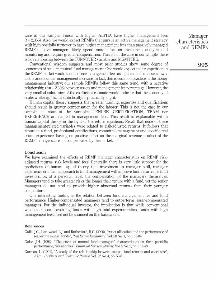
Managercharacteristicsand REMFs
995
case in our sample. Funds with higher ALPHA have higher management fees(t= 2.355). Also, we would expect REMFs that pursue an active management strategywith high portfolio turnover to have higher management fees than passively managedREMFs; active managers likely spend more effort on investment analysis andmonitoring and require greater compensation. This is not the case in our sample; thereis no relationship between the TURNOVER variable and MGMTFEE.
Conventional wisdom suggests and most prior studies show some degree ofeconomies of scale in mutual fund management. One would expect that competition inthe REMFmarket would tend to force management fees as a percent of net assets loweras the assets under management increase. In fact, this is common practice in the moneymanagement industry; our sample REMFs follow this same trend, with a negativerelationship (t=�2.308) between assets and management fee percentage. However, thevery small absolute size of the coefficient estimate would indicate that the economy ofscale, while significant statistically, is practically slight.
Human capital theory suggests that greater training, expertise and qualificationsshould result in greater compensation for the laborer. This is not the case in oursample, as none of the variables TENURE, CERTIFICATION, TEAM norEXPERIENCE are related to management fees. This result is explainable withinhuman capital theory in the light of the return equations. Recall that none of thesemanagement-related variables were related to risk-adjusted returns. It follows thattenure at a fund, professional certifications, committee management and specific realestate experience, having no positive effect on the marginal revenue product of theREMFmanagers, are not compensated by the market.
ConclusionWe have examined the effects of REMF manager characteristics on REMF risk-adjusted returns, risk levels and fees. Generally, there is very little support for thepredictions of human capital theory that investment in manager skill, managerexperience or a team approach to fund management will improve fund returns for fundinvestors, or, at a personal level, the compensation of the managers themselves.Managers tend to take greater risks the longer their tenure with a fund, yet the seniormanagers do not tend to provide higher abnormal returns than their youngercompetitors.
One interesting finding is the relation between fund management fee and fundperformance. Higher-compensated managers tend to outperform lesser-compensatedmanagers. For the individual investor, the implication is that while conventionalwisdom supports avoiding funds with high total expense ratios, funds with highmanagement fees need not be shunned on this basis alone.
References
Gallo, J.G., Lockwood, L.J. and Rutherford, R.C. (2000), ‘‘Asset allocation and the performance ofreal estate mutual funds’’, Real Estate Economics, Vol. 28 No. 1, pp. 165-84.
Golec, J.H. (1996), ‘‘The effect of mutual fund managers’ characteristics on their portfolioperformance, risk and fees’’, Financial Services Review, Vol. 5 No. 2, pp. 133-48.
Gorman, L. (1991), ‘‘A study of the relationship between mutual fund returns and asset size’’,Akron Business and Economic Review, Vol. 22 No. 4, pp. 53-61.

MF32,12
996
Kallberg, J.G., Liu, C.L. and Trzcinka, C. (2000), ‘‘The value added from investment managers: anexamination of funds of REITs’’, Journal of Financial and Quantitative Analysis, Vol. 35 No.3, pp. 387-408.
Lin, C.Y. and Yung, K. (2004), ‘‘Real estate mutual funds: performance and persistence’’, Journal ofReal Estate Research, Vol. 26 No. 1, pp. 69-94.
O’Neal, E.S. and Page, D.E. (2000), ‘‘Real estate mutual funds: abnormal performance and fundcharacteristics’’, Journal of Real Estate Portfolio Management, Vol. 6 No. 3, pp. 239-47.
Corresponding authorJames Philpot can be contacted at: [email protected]
To purchase reprints of this article please e-mail: [email protected] visit our web site for further details: www.emeraldinsight.com/reprints

The strongbuilding
997
Managerial FinanceVol. 32 No. 12, 2006
pp. 997-1002# Emerald Group Publishing Limited
0307-4358DOI 10.1108/03074350610710490
The strong building: a case studyin direct investment
Walt A. NelsonMissouri State University, Spring Field, Missouri, USA
Abstract
Purpose – The purpose of this case study is to examine direct investment in commercial real estatefrom the perspective of the individual. While most research is dominated by studies concerning directinvestment by institutions (REITs, pension funds, etc.), the bulk of direct investment in commercialproperty is still conducted by individuals.Design/methodology/approach – The paper presents accounting and financial data from theoriginal purchase, management and disposal of a small-scale office building. Cash flows, returns andrisks are measured and analyzed.Findings – The case demonstrates that successful direct investments may be characterized by short-term time horizons involving older, small-scale properties.Practical implications – This case illustrates the non-academic nature of real world directinvestment in commercial property. The case demonstrates that emotion and good timing are just asimportant to a successful venture as are cash flows and thorough risk estimates. The case also showsthat successful direct investment in commercial property may be limited to smaller, older propertiesheld for short-term time horizons.Originality/value – This case study is unique because it identifies the property, the investor, thepurchase price, the operating revenues and the sale price and net proceeds. Most case studies concealmany of these facts in order to preserve anonymity.
Keywords Real estate, Direct investment, Buildings
Paper type Case study
IntroductionDirect investment in real estate dominates the marketplace in the USA. The totalmarket value of equity in US commercial real estate in 2003 was approximately $2.5trillion (Ling and Archer, 2005, pp. 383 ff). Of this total, just 6.5 per cent ($168 billion)was held in publicly traded form, while the balance of almost $2.4 trillion was privatelyheld.Of this $2.4 trillion about 90 per cent ($2.166 trillion) was held by non-institutionalinvestors, i.e. direct investors. Direct investment offers the individual investor moreleverage, higher returns, more control and useful tax benefits (in certain tax brackets).Direct investment avoids the fee structure and dilution of returns which accompanyindirect investment.
The ‘‘A-list’’ of wealthy Americans who have invested directly in real estate includesJohn Rockefeller, Joseph Kennedy, Ted Turner, Arnold Schwarzenegger, Sam Zell,Donald Trump and George Steinbrenner, to name but a few. The reader will discover,after a little research, that many of these individuals made their initial fortunes involatile industries such as energy, securities and entertainment. Seeking stability, theyinvested much of their wealth in commercial real estate. It seems that, having made ahigh return ‘‘on’’ their initial investments, these individuals shifted their attention toeither preservation or return ‘‘of’’ capital by investing in real estate.
There is another way to look at the question of direct investment. Someone has toown and operate the commercial and residential rental property that is unsuitable forREIT funds. The strong building case looks at direct investment from the perspectiveof a real investor. The case identifies the property, the investor (the author of the case)and the financial details. It is a story presented within the complete cycle of property
The current issue and full text archive of this journal is available atwww.emeraldinsight.com/0307-4358.htm

MF32,12
998
ownership over a period of eight months: making the purchase, operating the propertyand selling the property. A section which discusses the estimation of the risks involvedis also included.
Making the purchaseIn late summer of 1978, I traveled to Beloit, Wisconsin to see an ‘‘investmentopportunity’’. The property was located in the heart of downtown. The strong building,as it was called, was constructed in the art deco style and built in the 1920s. Thebuilding had four floors and a basement, a portion of which was rentable. There were24 office and retail units and about two-thirds occupied. The list of tenants included aunion, various attorneys and insurance agents, a beauty shop, a barber shop,physicians, a dentist, an accountant and a stock broker. The structure had about 10,000square feet, and roughly 8,800 were rentable. The roof was flat, recently rebuilt and didnot leak. Parking was limited to a few spaces in front of the property and a city parkinglot about 200 feet behind the building. The furnace ran on natural gas. It was old and itleaked – money. The gas bills were so high an investor or property manager could beforgiven for thinking it might be more efficient just to shovel paper dollars into theboiler. Cash flows looked to be enough to cover the loan payment and operatingexpenses as long as I did not pay myself a salary to manage the place.
Beloit is located in Rock County, Wisconsin, along the Wisconsin-Illinois state line.It is located at the junction of I-90 and I-43 about 75 miles southwest of Milwaukee, 100miles northwest of Chicago, and 10 miles north of Rockford, Illinois, an importantmanufacturing regional city. In 1978 40 per cent of area workers were employed by themanufacturing, warehousing and distribution divisions of such Fortune 500 firms asBeatrice Foods, Taylor Freezer, Frito-Lay, Warner Electric Brake & Clutch. andHormel. Dairy farming was the second important industry next to manufacturing. Thepopulation of the city of Beloit was 35,000 at the time.
The economic environment in 1978-1979 was one of total confusion as Americanslearned for the second time in five years about the scandalous relationship between oiland interest rates. Inflation raged at an annualized rate of more than 10 per cent.Business loans and home mortgages cost between 9.5 per cent and 10 per cent. Goldpushed past $250, beef prices doubled, and the Iranian oil minister predicted oil at $35to $50 per barrel.
Table I shows that I paid $130,000 for the property with a down payment of $15,000,but the effective cash outflow was only a thousand bucks. I purchased the property
Table I.Strong building closingstatement: purchaseSeptember 1978
Seller credit ($) Buyer credit ($)
Purchase price 130,000Down payment 15,000Pro-rationsReal estate tax 1,714Special assesments 404Rents 1,161Elevator contract 55Trash contract 16Hazard insurance 314
Totals ($) 130,314 18,350Land contract to balance 111,964

The strongbuilding
999
through a closely-held corporation (I was the only stockholder). The corporationborrowed $9,000 from relatives (at 12 per cent interest) and I also persuaded the brokerto forego his commission in exchange for a company note in his favor of $5,000. Aftercredits on the closing statement were applied, the sellers financed the balance ofaround $112,000 via a land contract bearing interest at 9.8 per cent for 30 years with aballoon payment due at the end of five years. Monthly payments were $1,050. Theequity stake of $1,000 against a purchase price of $130,000 makes the LTV work out to0.993. Financial leverage indeed.
Operating the propertyThe building produced positive cash flows as shown in Table II. The only caveat is thatthe utility system generated high costs in winter which had to be offset by summersavings. Since I took over the ownership in the fall, there were no savings to work with.In order to cover winter heating expenses, I put the property on deferred billing withthe gas company.
The property also achieved positive financial leverage, generating eight months ofnet operating cash flows totaling $13,535. This number converts to an annual NOIof $20,300 ($20,300 = $13,535�12/8) or 15.6 per cent annualized overall rate of return(0.156 = $20,300/$130,000). The monthly NOI and before tax cash flow (BTCF) areshown in Table III. The cash on cash return from operations is calculated by dividingthe BTCF by the equity invested. Against the initial equity stake of $1,000, the BTCFreturned $5,138 during the eight months of operation. The raw return is 513.8%.Multiplying 513.8 by 12/8 annualizes the return at 770.7%, which probably qualifies asentry level loan sharking. Both the ROR of 15.6 per cent and the cash-on-cash ROE of770% exceed the rate paid to the underlying loan of 9.8 per cent. The impact of thedeferred gas billing is picked up in the closing statement.
Selling the propertyWith such great returns from operations, why sell? First, I lacked a good marketingplan to fill up the vacant offices. Second, I lacked the time to execute such a plan, due to
Table II.Strong building
operating cash flows:October 1978
Gross potential income $3,997Less vacancies �1,085
Effective gross income 2,912ExpensesElevator inspection 86Trash service 25Cleaning 54Supplies 111Ads 11Repairs 279Utilities 502Property tax and assessments 222Miscellaneous 23
1,313
NOI 1,599Debt service 1,050
BTCF $549

MF32,12
1000
other business ventures. Third, there was an offer on the table. The real estate brokerwho had sold me the property called to say he had a contract to buy us out. He askedme to prepare an annualized pro forma income statement for the property.
The gross potential income for the property was $47,820 per year, but due tovacancies the effective gross income was about $2,900 per month or $34,800 per year.However, the strong building held the potential for much more, as shown in the Proforma in Table IV. Assuming that a marketing plan would reduce vacancies to 10 percent and allocating an additional $4,800 per year toward capital improvements toupdate the premises, the property still had the ability to generate a NOI of over $22,000per year. Table IV shows that capitalized at 12 per cent, the NOI of $22,520 indicates aproperty value of more than $187,000.
In April 1979 a group of investors paid $156,000 for the property. Table V showsthat the ‘‘gross-net’’ from the sale was over $40,000. However, Table VI shows that the‘‘net-net’’ was just under $23,000 by the time all of the bills and loans were paid.
Adding the net from the settlement with the broker to the $5,138 from operationsproduces a total BTCF of $28,118 ($22,980 + $5,138). Against the $1,000 equity stake,this amounts to an ROE of more than 2,800%, which exceeded the 1978-1979 T-Bill rateof just under 9 per cent.
Estimating the riskIt is always best to estimate risk before investing money. In this case, the ex ante riskestimate considered the vacancy rate of the building, the time involved to operate and
Table III.Summary of monthlyoperating cash flows
NOI ($) Month BTCF ($)
1,599 September 5491,599 October 5491,829 November 7802,149 December 1,0991,914 January 8651,446 February 3961,133 March 831,866 April 817
13,535a 5,138a
Note: aWinter gas bills were deferred until May and totaled $3,000
Table IV.Selling the pro formapotential of the strongbuilding
Gross potential income $47,820Less hypothetical vacancies of 10% �4,800
Effective gross income $43,020Less current operating expenses �15,700Less capital improvements �4,800
Net operating income $22,520Less current debt service �12,600
Before tax cash flow $9,920Indicated property value (NOI/0.12) $187,666

The strongbuilding
1001
market the property weighed against the probable disappointment of the relative whohad suggested I make the purchase. That relative was my father – a seasoned realestate entrepreneur. Not wishing to disappoint him weighed more heavily than therisks of making the purchase, so logic lost out to emotion and I bought the place. It maynot be academic, but it is the real world.
Table V.Strong building closing
statement: saleApril 1979
Seller credit ($) Buyer credit ($)
Purchase price 156,000Down payment 3,000Recording fee 3Pro-rationsReal estate tax 635Special assesments 152Rents 1,286Elevator contract 52Trash contract 16
Supplies 55Hazard insurance 535
Totals ($) 156,590 5,144Less buyer credits �5,144
Sub-total 151,446Assignment of land contract �111,134Cash due at closing from buyer ($) 40,312
Table VI.Broker’s settlementstatement: strong
building April 1979
Balance from closing due seller $40,312Down payment 3,000
Sub-total $43,312Charges against sellerPro-ration of accrued interest on land contract($111,134�0.098)/360 = $30.25 per day$30.25�30 days (from 3/19) = $908Title insurance 465Gas company (deferred gas billing) 3,854Legal 85Commission 5,300
Sub-total $10,612Less charges against seller �10,612
Cash due seller $32,700Pay off loan and eight month interest to relative �9,720
BTCF from sale of strong building $22,980
Table VII.CAPM estimate of
riskiness � (beta) for thestrong building
4,217%=9%+ ß(18.6%�9%)4,217%=9%+9.6%ß4,208%=9.6%ß438.3 = ß

MF32,12
1002
However, it is still possible to estimate the risk of the strong building after the factusing the capital asset pricing model (CAPM). In 1979 the risk free rate for one-yearTreasury bills was about 9 per cent. The ‘‘market’’ rate of return was about 1 per centbecause the Dow languished from 811 in January 1979 to 824 in January 1980. A bettermeasure of market returns is the FRC/NCREIF index for real estate commercialproperty during 1979, which was 18.6 per cent (Dasso et al., 1995, p. 62). The strongbuilding returned an astounding 4,217% annualized (4,217%=2,811%�12/8).Therefore, it is possible to estimate ß (beta) or the risk level as shown in Table VII.
The � (beta) of 438 indicates the strong building investment carried 438 times therisk of the average real estate investment included in the NCREIF index. High risk,high return. I never paid myself a salary during my tenure as landlord. Evensupposing I had paid myself as much as $12,000 (a grand a month was decent moneyin 1978), and subtracting this from the $28,118 leaves a return of $16,118 – a mere1,600% rate of return.
ConclusionsREITs offer stabilized cash flows through diversified property investment on a massivescale. Unfortunately, REIT share prices constantly change to reflect the impact ofinterest rates and other factors. Some investors may be troubled by the fact that thesecurities issued against real property trade in a market which is more volatile than theunderlying properties. Direct investment provides no diversification until the investorhas purchased a number of properties, but it does provide stability in terms of propertyvalue, because the investor is not required to report changes in property value on acontinuous basis. That is, no property index is found on the front of the subjectproperty to reflect ever instantaneous change in value. The strong building caseillustrates the non-academic nature of real world direct investment in commercialproperty. The case demonstrates that emotion and good timing are just as important toa successful venture as are cash flows and thorough risk estimates. The case alsoshows that successful direct investment in commercial property may be limited tosmaller, older properties held for short-term time horizons.
References
Dasso, J.E., Shilling, J.D. and Ring, A.A. (1995), Real Estate, 12th ed., Prentice-Hall, EnglewoodCliffs, NJ.
Ling, D.C. and Archer, W.R. (2005), Real Estate Principles: A Value Approach, McGraw-Hill Irwin,New York, NY.
Corresponding authorWalt A. Nelson can be contacted at: [email protected]
To purchase reprints of this article please e-mail: [email protected] visit our web site for further details: www.emeraldinsight.com/reprints


