arX

iv:1

208.

5003

v2 [

cs.L

G]

27 A

ug 2

012

1Identification of Probabilities of LanguagesPaul M.B. Vitanyi and Nick Chater

Abstract

We consider the problem of inferring the probability distribution associated with a language, given

data consisting of an infinite sequence of elements of the languge. We do this under two assumptions on

the algorithms concerned: (i) like a real-life algorothm ithas round-off errors, and (ii) it has no round-

off errors. Assuming (i) we (a) consider a probability mass function of the elements of the language if

the data are drawn independent identically distributed (i.i.d.), provided the probability mass function is

computable and has a finite expectation. We give an effectiveprocedure to almost surely identify in the

limit the target probability mass function using the StrongLaw of Large Numbers. Second (b) we treat

the case of possibly incomputable probabilistic mass functions in the above setting. In this case we can

only pointswize converge to the target probability mass function almost surely. Third (c) we consider

the case where the data are dependent assuming they are typical for at least one computable measure

and the language is finite. There is an effective procedure toidentify by infinite recurrence a nonempty

subset of the computable measures according to which the data is typical. Here we use the theory of

Kolmogorov complexity. Assuming (ii) we obtain the weaker result for (a) that the target distribution is

identified by infinite recurrence almost surely; (b) stays the same as under assumption (i). We consider

the associated predictions.

I. INTRODUCTION

In cognition and science one learns by observation. The perceptual system of an individual person, or

the data-gathering resources of a scientific community, incrementally gathers empirical data, and attempts

to find the structure in that data. The question arises: underwhat conditions is it possiblepreciselyto

infer the structure underlying those observations? Or, relatedly, under what conditions could a machine

learning algorithm potentially precisely recover this structure? We can model this problem as having

Vitanyi is with the national research institute for mathematics and computer science in the Netherlands (CWI) and theUniversity of Amsterdam. Address: CWI, Science Park 123, 1098 XG, Amsterdam, The Netherlands. Email:paulv@cwi.nl.

Chater is with the Behavioural Science Group. Address: Warwick Business School, University of Warwick, Coventry,CV4 7AL, UK. Email: Nick.Chater@wbs.ac.uk. Chater was supported by ERC Advanced Grant “Cognitive and SocialFoundations of Rationality.”

DRAFT

the following form: given a semi-infinite sequence of samples from a probability distribution, under

what conditions is it possible precisely to recover this distribution? Moreover, we can focus on the case

where each observation is coded in a language—that is, each observation corresponds to an element

of a countable set of sentences. Then the problem at hand is torecover the probability induced by the

language.

In the context of the cognitive processes of an individual, information from the senses is presumed to

be coded in the brain to some finite precision (indeed, neuralfiring is discrete, [19]). Linguistic input, in

particular, can be coded in a hierarchy of discrete symbolicrepresentations, as described by generative

grammar (for example, [12]). And, in the context of the operation of the scientific community, data is

digitally coded to finite precision in symbolic codes. Thereare at least three reasons for scepticism that

precisely recovering the probability of possible observations is possible.

First, as observed by Popper [17], however much data has beenencountered, any theory or model can

be falsified by the very next piece of data. However many whiteswans are observed, there is always

the possibility that the very next swan will be black, or somemore unlikely color. If, in the case of

a child learning a language, however often the child encounters sentences following a particular set of

grammatical rules, it is always possible that the very next sentence encountered will violate these rules

(for example [16]). Thus, however, much data been encountered, there is no point at which the learner can

announce a particular probability as correct with any certainty. But this does not rule out the possibility

that the learner might learn to identify the correct probability in the limit. That is, perhaps the learner

might make a sequence of guesses, finally locking on to correct probability and sticking to it forever—

even though the learner can never know for sure that it has identified the correct probability successfully.

We shall therefore consider identification in the limit below (following, for example, [5], [8], [16]).

Second, in conventional statistics, probabilistic modelsare typically idealized as having continuous

valued parameters; and hence there is an uncountable numberof possible probabilities, from which the

correct probability is to be recovered. In general it is impossible that a learner can make a sequence of

guesses that precisely locks on to the correct values of continuous parameters. This, since the possible

strategies of learners are effective in the sense of Turing [20] and thus countable. This assumption is,

of course, obeyed by any practical machine learning algorithm and we assume also by the brain. The

set of such strategies can express only a countable number ofpossible hypotheses. From this mild

assumption, it is, of course, immediately evident that the overwhelming majority of a continuum of

hypotheses cannot be represented, let alone learned. Moreover, there is a particularly natural restriction

2

concerning the set of probabilites from which the learner chooses: it must becomputable(these notions

are made precise below). This seems a reasonable restriction, both in cognitive science and scientific

methodology. After all, the assumption that individual human information processing is computable is a

founding assumption of cognitive science (see for example,[18]); and the same constraint arguably applies

to every practically usable scientific theory (although whether this holds is discussed in [2]). We shall

see below that restricting ourselves to the computable simplifies the problem of precisely reconstructing

the correct probability from the observed data. For example, the computability of the set of possible

probabilities means that these can be enumerated; and it maythen be possible to gradually home in the

correct probability, by successively eliminating earlierones in the enumerated list. As we see below, it

is also possible to provide approximation results if the computability restriction is dropped.

A third reason for initial scepticism also concerns computability—this time for the learner, not just

the probability to be recovered. Even if there is, in principle, sufficient data to pin down the correct

probability precisely, there remains the question of whether there is a feasible computational procedure

that can reliably map from data to a sequence of guesses that eventually lock on to the correct probability.

Real-life computational procedures are finite and always have round-off errors. We outline positive results

that can be obtained for computable learners with or withoutsuch round-off errors.

A. Preliminaries

A language is a set of sentences. The learnability of a language under various computational

assumptions is the subject of an immensely influential approach in [4] and especially [5]. But surely

in the real world the chance of one sentence of a language being used is different from another one. For

example, many short sentences have a larger chance of turning up than very long sentences. Thus, the

elements of a given language are distributed in a certain way. There arises the problem of identifying or

approximating this distribution.

We first introduce some terminology. A function iscomputable, if there is a Turing machine (or

any other equivalent computational device such as a universal programming language) that maps the

arguments to the values. We say that weidentify a functionf in the limit if we effectively produce an

infinite sequencef1, f2, . . . of functions andfi = f for all but finitely manyi. This corresponds to the

notion of “identification in the limit” in [5]. Weidentify a functionf by infinite recurrenceif fi = f for

infinitely manyi. A sequence of functionsconverges toa functionf pointswizeif limi→∞ fi(a) = f(a)

for all a in the domain off . The functions we are interested in are versions of the probability mass

3

functions.

The restriction to computable probability mass functions (or more generally any restriction to a

countable set of probability mass functions) is both cognitively realistic (if we assume language is

generated by a computable process) and dramatically simplifies the problem of language identification.

This is also the case for the use of algorithms with round-offerrors.

B. Related work

In [1] (citing previous more restricted work) a target probability mass function was identified in the

limit when the data are drawn independent identically distributed (i.i.d.) in the following setting. Let the

target probability mass functionp be an element of a listq1, q2, . . . subject to the following conditions: (i)

everyqi : N → R+ is a probability mass function whereN andR+ denote the positive natural numbers

and the positive real numbers, respectively; (ii) there is atotal computable functionC(i, x, ǫ) = r such

that (qi(x) − r) ≤ ǫ with r, ǫ > 0 are rational numbers. The technical means used are the Law ofthe

Iterated Logarithm and the Kolmogorov-Smirnov test. The algorithms used have no round-off errors.

However, the listq1, q2, . . . cannot contain all computable probability mass functions,Lemma 4.3.1 in

[14].

C. Results

In Section II we deal with probability mass functions. For technical reasons we introduce a weaker form

thereof called “semiprobability mass functions.” Consider a probability mass function satisfying (A.1)

below associated with a language. The data consist of an infinite sequence of elements of this language that

are drawn i.i.d. The aim is to identify the probability mass function given the data. (In contrast to [1] we

allow all computable probability mass functions.) In Section II-A we consider algorithms without round-

off errors. Then, we identify the target distribution by infinite recurrence almost surely. In Section II-B

the identification algorithm is subject to round-off errorsand we identify the target distribution in the

limit almost surely (underpinning the result announced in [7]). In Section III we treat the case of possibly

uncomputable probability mass functions. Then we can only show pointswize convergence almost surely.

This result holds both with or without round-off errors. Thetechnical tool in these sections is the Strong

Law of the Large Numbers. In all these results the language concerned can be infinite. In Section IV

we consider the case where the data are dependent assuming they are typical (Definition 9) for at least

one computable measure. In contrast to the i.i.d. case, it ispossible that the data are typical for many

4

measures. The language concerned is finite and the identification algorithm has round-off errors. Then,

we identify by infinite recurrence (possibly a subset) of computable measures for which the data are

typical. The technical tool is Kolmogorov complexity. Finally, In Section V we consider the associated

predictions. We defer the proofs of the theorems to AppendixA.

II. COMPUTABLE PROBABILITY MASS FUNCTIONS

Most known probability mass functions are computable provided their parameters are computable. In

order that it is computable we only require that the probability mass function is finitely describable and

there is an effective process producing it [20].

It is known that the overwhelming majority of real numbers are not computable. An example of

an incomputable probability mass function therefore is theone associated with a biased coin with an

incomputable probabilityp of outcome heads and probability1− p of outcome tails,0 ≤ p ≤ 1. On the

other hand, ifp is lower semicomputable, then we can effectively find nonnegative integersa1, a2, . . .

andb1, b2, . . . such thatan/bn ≤ an+1/bn+1 and limn→∞ an/bn = p. Let us generalize this observation.

DEFINITION 1: If a function has as values pairs of nonnegative integers,such as(a, b), then we can

interpret this value as the rationala/b. This leads to the notion of a computable function with rational

arguments and real values. A real functionf(x) with x rational is semicomputable from belowif it

is defined by a rational-valued total and computable function φ(x, k) with x a rational number and

k a nonnegative integer such thatφ(x, k + 1) ≥ φ(x, k) for every k and limk→∞ φ(x, k) = f(x).

This means thatf can be computably approximated arbitrary close from below (see [14], p. 35). A

functionf is semicomputable from aboveif −f is semicomputable from below. If a real function is both

semicomputable from below and semicomputable from above then it is computable. A function f is a

semiprobabilitymass function if∑

x f(x) ≤ 1 and it is aprobability mass function if∑

x f(x) = 1. It

is customary to writep(x) for f(x) if the function involved is a semiprobability mass function.

We cannot effectively enumerate all computable probability mass functions (this is a consequence

of Lemma 4.3.1 in [14]). However, it is possible to enumerateall and only the semiprobability mass

functions that are lower semicomputable. This is done by fixing an effective enumeration of all Turing

machines of the so-calledprefix type. (Such an enumeration is quite the same as effectively enumerating

all programs in a conventional computer programming language that is computationally universal and

were the programs are prefix-free—a set is prefix-free if no element is a proper prefix of any other. Most,

5

if not all, conventional computer programming languages satisfy these requirements.) It is possible to

change every Turing machine description in the enumerationinto one that computes a semiprobability

mass function that is computable from below, Theorem 4.3.1 in [14] (originally in [21], [13]). The result

is

Q = q1, q2, . . . , (II.1)

a list containing all and only semiprobability mass functions that are semicomputable from below. Without

loss of generality every element ofQ is over the alphabetL.

DEFINITION 2: There is a total and computable functionφ(i, x, t) = qti(x) such thatφ(i, x, t) ≤

φ(i, x, t + 1) and limt→∞ qti(x) = qi(x).

Every probability mass function is a semiprobability mass function, and every computable probability

mass function is semicomputable from below. Therefore, every computable probability mass function is in

list Q. Indeed, every such function will be in the list infinitely often, which follows simply from the fact

that there are infinitely many computer programs that compute a given function. If a lower semicomputable

semiprobability mass function is a probability mass function, then it must be computable, [14] Example

4.3.2. Therefore, every probability mass function in the list is computable. It is important to realize that,

although the description of every computable probability mass function is in listQ, it may be there in

lower semicomputable format and we may not know it is computable.

A. Algorithms Without Round-Off Errors

DEFINITION 3: Let x = x1, x2, . . . be an infinite sequence of elements of the languageL i.i.d. drawn

according to a computable probability mass functionp. Let Q(p) be defined as the set of indices of

elements ofQ that are copies ofp.

THEOREM 1: COMPUTABLE I.I.D. PROBABILITY IDENTIFICATION (NO ROUND-OFF) Let L be a

language{a1, a2, . . .} (a countably finite or infinite set) with a computable probability mass function

p. Without loss of generality we assume that everya ∈ L is a finite integer. Let the mean ofp exist

(∑

a∈L ap(a) < ∞). The algorithm in the proof takes as input an infinite sequence x = x1, x2, . . . of

elements ofL drawn i.i.d. according top. After processingxn the algorithm computes as output the

index in of a semiprobability mass function in the enumerationQ. DefineQ∞ as the set of indices of

elements inQ that appear infinitely often in the sequence produced by the algorithm. Then,

(i) Q∞ 6= ∅ almost surely;

(ii) if i ∈ Q∞ then i ∈ Q(p) almost surely; and

6

(iii) almost surelylim infn→∞ in = minQ(p).

B. Algorithms With Round-Off Errors

We will want to computationally separate probability mass functionsp for which∑

x p(x) = 1 from

semiprobability mass functionsq for which∑

x q(x) < 1 in the listQ.

DEFINITION 4: To deal with truncation errors in the above (in)equalities we use the following notation.

The truncation error is a known additive term±ǫ, ǫ > 0, and we denote (in)equalities up to this truncation

error by+

≤,+

≥,+=,

+<, and

+>. Every function that satisfies the probability mass function equality within

the round-off error is viewed as a probability mass function.

Let L be a language{a1, a2, . . .}, #a(x1, x2, . . . , xn) be the number of elements inx1, x2, . . . , xn equal

a ∈ L, andk′ be the least index of an elementqi in the listQ such that

limn→∞

n∑

j=1

∣

∣

∣

∣

qi(aj)n −

#aj(x1, x2, . . . , xn)

n

∣

∣

∣

∣

+= 0.

THEOREM 2: COMPUTABLE I.I.D. PROBABILITY IDENTIFICATION (ROUND-OFF) Let L be a lan-

guage{a1, a2, . . .} (a countably finite or infinite set) with a computable probability mass functionp.

Without loss of generality we assume that everya ∈ L is a finite integer. Let the mean ofp exist

(∑

a∈L ap(a) < ∞). The algorithm in the proof takes as input an infinite sequence x = x1, x2, . . . of

elements ofL drawn i.i.d. according top. After processingxn the algorithm computes as output the

index in of a semiprobability mass function in the enumerationQ. There exists anN such thatin = k′

for all n ≥ N . We havek′ ≤ k with k as in Theorem 1.

III. G ENERAL PROBABILITY MASS FUNCTIONS

Can we get rid of the restriction that the probability mass function be computable? Above we used the

computability to consider a well-ordered countable list oflower semicomputable semiprobability mass

functions, and pin-pointed the least occurrence of the target in the list. We use the fact that we have a

guarantee that the target is in the list. If we have no such guarantee (possibly there is no list), we can

still converge pointswise to theempirical probability mass function of the languageL based on the data

x1, x2, . . . . We do this by an algorithm computing the probabilityp(a) in the limit for all a ∈ L.

Note that this is quite different from Theorems 1, 2. There weindicated (the least occurrence of)p

precisely in a well-ordered list even though the result onlyholds “almost surely.” In contrast, here we find

7

p(a) for all a ∈ L in the limit only. Moreover, this holds also “almost surely.” However, the probability

mass functions considered here consist ofall probability mass functions onL—computable or not.

THEOREM 3: I.I.D. PROBABILITY APPROXIMATION WITH AN ALGORITHM WITHOUT ROUND-OFF

ERROR Let L be a language{a1, a2, . . .} (a countably finite or infinite set) with a computable probability

mass functionp. Without loss of generality we assume that everya ∈ L is a finite integer. Let the mean

of p exist (∑

a∈L ap(a) < ∞). The algorithm in the proof takes as input an infinite sequencex1, x2, . . .

of elements ofL drawn i.i.d. according top. After processingxn the algorithm computes as output a

probability mass functionpn. Almost surely for alla ∈ L the limn→∞ pn(a) = p(a).

With round-off error this theorem is about the same.

REMARK 1: Can this result be strengthened to a form of dependent variables? It all depends on

whether the Strong Law of Large Numbers holds. We know from [3], p. 474, that the Strong Law of

Large Numbers holds for stationary ergodic sources with finite expected value. ✸

IV. COMPUTABLE MEASURES

This time let the languageL = {a1, a2, . . . , am} be a finite set, andx1, x2, . . . the data consisting of an

infinite sequence of elements fromL. We drop the requirement of independency of the different elements

in the data. Thus, we assume that our data sequencex1, x2, . . . is possibly dependent. This implies that

the probability model forL is more general than i.i.d.. In fact, we will allow all computable measures on

the infinite sequences of elements fromL. Thus, the probability model used includes stationary processes,

ergodic processes, Markov processes of any order, and othermodels, provided they are computable.

Given a finite sequencex = x1, x2, . . . , xn of elements of the basic setL, we consider the set of infinite

sequences starting withx. The set of all such sequences is written asΓx, thecylinderof x. We associate

a probabilityµ(Γx) with the event that an element ofΓx occurs. Here we abbrieviateµ(Γx) to µ(x).

The transitive closure of the intersection, union, complement, and countable union of cylinders gives a

set of subsets ofL∞. The probabilities associated with these subsets are derived from the probabilities

of the cylinders in standard ways [9]. Asemimeasureµ satisfies the following:

µ(ǫ) ≤ 1 (IV.1)

µ(x) ≥∑

a∈L

xa,

and if equality holds instead of each inequality we callµ a measure. Using the above notation, a

semimeasureµ is lower semicomputableif it is defined by a rational-valued computable function

8

φ(x, k) with x ∈ L∗ and k a nonnegative integer such thatφ(x, k + 1) ≥ φ(x, k) for every k and

limk→∞ φ(x, k) = µ(x). This means thatµ can be computably approximated arbitrary close from below

for each argumentx ∈ L∗.

To separate measures from semimeasures that are not measures using an algorithm subject to round-off

errors, we have to deal with truncation errors in the (semi)measure (in)equalities. This truncation error

is a known additive term±ǫ, ǫ > 0. Again we use Definition 4: (in)equalities up to this truncation error

are denoted by+

≤,+

≥,+=,

+<, and

+>.

In the argument below we want to effectively enumerate all computable measures. By Lemma 4.5.1

of [14], if a lower semicomputable semimeasure is a measure,then it is computable. Thus it suffices

to effectively enumerate all lower semicomputable measures. By Lemma 4.5.2 of the cited reference

this is not possible. But if we effectively enumerate all lower semicomputable semimeasures, then this

enumeration includes all lower semicomputable measures which are a fortiori computable measures.

This turns out to be possible (originally in [21], [13]). Just as in the case of lower semicomputable

semiprobabilities, but with a little more effort, we can effectively enumerate all and only lower

semicomputable semimeasures, as is described in the proof of Theorem 4.5.1 of [14]. This goes by taking

a standard enumeration of all Turing machinesT1, T2, . . . of the so-calledmonotonetype. Subsequently

we transform every Turing machine in the list to one that lower semicomputes a semimeasure. Also, it

is shown that all lower semicomputable semimeasures are in the list. The result is

M = µ1, µ2, . . . . (IV.2)

This list contains all and only semimeasures that are semicomputable from below. It is important to

realize that, although the description of every computablemeasure is in listM, it may be there in lower

semicomputable format and we may not know it is computable.

DEFINITION 5: There is a total and computable functionφ(i, x, t) = µti(x) such thatφ(i, x, t) ≤

φ(i, x, t + 1) and limt→∞ µti(x) = µi(x).

REMARK 2: Let our data bex1, x2, . . . . Possibly there are none or more than one computable measures

that have these data as a “typical” sequence. Here we use “typicality” according to the Definition 9

below. Such typical infinite sequences are also called “random” with respect to the measure involved.

For instance, let the data sequence be0, 0, . . . . Then this is a typical sequence of the computable measure

µi1 that gives measure 1 to every initial segment of this data sequence. But if we considerµi2 that gives

measure12

to every initial segment of0, 0, . . . and also measure12

to every initial segment of1, 1, . . . ,

9

then the considered data sequence is also a typical sequenceof µi2 . Similarly, it is a typical sequence

of the measureµik that gives measure1/k to every initial segment of0, 0, . . . throughk − 1, k − 1, . . .

(k < ∞).

Hence our task is not to identify the measure according to which the data sequence was generated as

a typical sequnce, but to identify measures whichcould have generated the data sequence as a typical

sequence. Note that we have reduced our task from identifying the computable measure generating the

data, which is not possible, tosomecomputable measures thatcouldhave generated the data as a typical

sequence. ✸

REMARK 3: We assume here thatL is finite. This is no genuine restriction since all real natural or

artificial languages that ever existed contain less than, say, 10100 elements. This is supported by the fact

that 10100 far exceeds the number of atoms currently believed to exist in the observable universe. We

assume thatL is finite since it makes the computation of∑

a∈L xa for x ∈ L∗ effective.

Where appropriate, we shall use the (in)equalities according to Definition 4. This has bad and good

effects. The bad effect is that semimeasures that violate the measure equalities by at most the truncation

error are counted as measures. The good effects are, besidescomputationally verifiable (in)equalities, that

in the infinite processes to construct lower semicomputablesemimeasures (the proof of Theorem 4.5.1

of [14]) we only need to consider finite initial segments. ✸

Let L be a language with a computable measureµ on the infinite sequences of its elements. We recall

the notion that an infinite sequencex is “typical” for µ.

DEFINITION 6: Let x = x1, x2, . . . be an infinite sequence of elements of the languageL. The infinite

sequencex is typical or randomfor a computable measureµ if it passes all effective sequential tests for

randomness with respect toµ in the sense of Martin-Lof [15]. The set of such sequences haveµ-measure

one. We defineM(x) as the set of indices of elements of the listM that are computable measuresµ

such thatx is typical forµ.

THEOREM 4: COMPUTABLE MEASURE IDENTIFICATION BY ALGORITHMS WITH ROUND-OFF ER-

RORSLet L = {a1, a2, . . . , am}, m < ∞, be a language and letx1, x2, . . . with xi ∈ L be an infinite data

sequence. Assume that the data sequence is typical for at least one computable measure. The algorithm

in the proof takes as input the infinite sequencex1, x2, . . . . After processingxn the algorithm computes

as output the indexin of an element ofM. DefineM∞ as the set of indices of elements inM that

appear infinitely often in the sequence produced by the algorithm. Then,M∞ ⊆ M(x), M∞ 6= ∅, and

|M∞| < ∞.

10

V. PREDICTION

In Sections II and III the data are drawn i.i.d. according to aprobability mass functionp on the

elements ofL. Given p, we can predict the probabilityp(a|x1, . . . , xn) that the next draw results in an

elementa when the previous draws resulted inx1, . . . , xn. (The same holds in appropriate form for a

good pointswise approximationp of p.)

For measures as in Section IV, allowing dependent data, the situation is quite different. In the first

place there can be many measures that havex = x1, x2, . . . as typical (random) data. In the second place,

different of these measures may give different probabilitypredictions using the same initial segment of

x.

Let us give a simple example. Suppose the data isx = a, a, . . . . This data is typical for the measureµ1

defined byµ1(x) = 1 for everyx consisting of a finite or infinite string ofa’s andµ1(x) = 0 otherwise.

But the data is also typical forµ2 which gives probabilityµ2(x) =12

for every string consisting of ana

followed by a finite or infinite string ofa’s, or a followed by a finite or infinite string ofb’s.

Firstly, µ1 is not equal toµ2, even thoughx is typical for both of them. Secondly,µ1(a|a) = 1. But

µ2(a|a) = µ2(b|a) =12. In fact, µ1(y|a) = 1 for everyy consisting of a finite or infinite string ofa’s,

and0 otherwise. The conditional probabilityµ2(y|a) is 12

for y consisting of a finite or infinite string of

a’s or y consisting of a finite or infinite string ofb’s, and0 otherwise. Thus, different measures for which

the data is typical may give very different predictions. With respect to predictions we can only proceed

as follows: (i) find one or more measures for which the data is typical, and (ii) predict according to one

of these measures that we select.

It does not seem make sense to make a weighted prediction according to the measures for which the

data is typical. There may not be a single measure among them making that prediction. Moreover, the

consecutive data resulting from many predictions may not betypical with respect to any of the original

measures.

The question arises how the i.i.d. case and the measure case relate to one another. The answer is as

follows. For ease of writing we will ignore the adjective “computable.” It is clear that the i.i.d. probabilities

are a subset of the more general case of measures. Containment is proper since there is a measure that

is not an infinite sequence of i.i.d. draws according to a probability mass function. An example is given

below.

Moreover, an infinite sequence of data can be typical for morethan one measure, even though if such

a sequence is typical for an infinite sequence of i.i.d. drawsof any probability mass function, then it

11

is typical for an infinite sequence of i.i.d. draws of only this single probability mass function. Thus, if

the data is typical for different measures, then only one of the measures involved is a probability mass

function.

Let us give an example. The measureµ1 above has a single typical sequencex = a, a, . . . . This measure

results from infinitely many i.i.d. draws ofL according to the probability mass functionp(a) = 1 and

p(z) = 0 for z ∈ L\{a}. But x is also typical forµ2, a measure which has no i.i.d. case that corresponds

to it. This can be seen as follows. The measureµ2 has also the typical sequencey = a, b, b, . . . , a sequence

such that no infinite number of i.i.d. draws of any probability mass function corresponds to it. Namely, the

probability of a andb must both be non-zero to yield the sequencey. Hence a typical infinite sequence

must contain (in the i.i.d. case) infinitelya’s andb’s. But y does not do so.

Thus, the i.i.d. case is a proper subset of the measure case. Asingle infinite sequence can be typical

for many (infinitely many) measures, even though if it is typical for an i.i.d. case it is typical for only a

single one of the probability mass functions. But there are infinite sequences that are typical for many

measures but not typical for any case of infinitely many i.i.d. draws according to a probability mass

function.

APPENDIX

Proof: OF THEOREM 1. Our data is, by assumption, generated by i.i.d. draws according to a

computable probability mass functionp satisfying (A.1). Formally, the datax1, x2, . . . is generated by a

sequence of random variablesX1,X2, . . . , each of which is a copy of a single random variableX with

probability mass functionP (X = a) = p(a) for everya ∈ L. Without loss of generalityp(a) > 0 for

all a ∈ L. The mean ofX exists by (A.1).

REMARK 4: In probability theory the statementalmost surelymeans “with probability one.” Let us

illustrate this notion. It is possible that a fair coin generates an infinite sequence0, 0, . . . even though

the probability of 1 at each trial is12. The uniform measure of the set of infinite sequences, such that

the relative frequency of 1’s goes to the limit12, is one. Call sequences in that setpseudo typical. The

probability that an infinite sequence is pseudo typical is one, even though there are infinite sequences (like

in the example above) that are not pseudo typical. Thus, “almost surely” may not mean “with certainty.”

✸

The Strong Law of Large Numbers (originally in [10]) states that if we perform the same experiment

a large number of times, then almost surely the average of theresults goes to the expected value. That

12

is, if a mild condition is satisfied. We require that our sequence of random variablesX1,X2, . . . satisfies

Kolmogorov’s criterion that∑

i

(σi)2

i2,

whereσ2i is the variance ofXi in the sequence of mutually independent random variablesX1,X2, . . . .

Since allXi’s are copies of a singleX, all Xi’s have a common distributionp. In this case we use the

theorem on top of page 260 in [6]. To apply the Strong Law in this case it suffices that the mean ofX

exists. (We denote this mean byµ, not to be confused with the notation of measuresµ(·) we use below.)

That is, we require that

µ =∑

a∈L

ap(a) < ∞. (A.1)

Then, the Strong Law states that

Pr

(

limn→∞

1

n

n∑

i=1

Xi = µ

)

= 1,

or (1/n)∑n

i=1Xi converges almost surely toµ asn → ∞.

To determine the probability of ana ∈ L we consider the related random variablesXa with just two

outcomes{a, a}. This Xa is a Bernoulli process(q, 1 − q) whereq = p(a) is the probability ofa and

1− q =∑

b∈L\{a} p(b) is the probability ofa. If we seta = min (L \ {a}) while the probability ofa is

1− q =∑

b∈L\{a} p(b), then the meanµa of Xa is

µa = aq + a(1− q) ≤ µ.

REMARK 5: Recall thatL may be infinite, that is,L = {a1, a2, . . . , }. Then a priori it could be that

limj→∞ µaj= ∞. But we have just proved that not only this does not happen butevenµaj

≤ µ for

everyj. ✸

Thus, everya ∈ L incurs a random variableXa for which the equivalent of (A.1) applies. Therefore,

according to the cited theorem the quantity(1/n)∑n

i=1(Xa)i converges almost surely toµa asn → ∞.

Therefore, almost surely

limn→∞

n∑

j=1

∣

∣

∣

∣

p(aj)−#aj(x1, x2, . . . , xn)

n

∣

∣

∣

∣

= 0. (A.2)

13

Algorithm (x1, x2, . . .):Step 1for n = 1, 2, . . . execute Steps 2 through 4.Step 2 SetI := ∅; for i := 1, 2, . . . , n execute Step 3.Step 3 setγi,n := 1; L: if

∑nj=1 |q

ni (aj)−#aj(x1, x2, ..., xn)/n| ≤ 1/γi,n

then (γi,n := γi,n + 1; goto L) else γi,n := γi,n − 1;if γi,n > γi,n−1, . . . , γi,1 then I := I

⋃

{i}.Step 4if I 6= ∅ then in := min I else in := in−1; output in.

Fig. 1. Algorithm 1a

With q 6= p substituted forp in the lefthand side of (A.2), we have that this left-hand side is almost

surely unequal0. Using some probability theory, we can rewrite the Strong Law using only the finite

initial segment of the infinite sequence of (copies of) the two-outcome random variables. We use ([6], p

258 ff). For every pairǫ > 0 and δ > 0, there is anN such that there is a probability1 − δ or better

that for everyr > 0 all r + 1 inequalities:∣

∣

∣

∣

p(a)−#a(x1, x2, . . . , xn)

n

∣

∣

∣

∣

≤ ǫ, (A.3)

with n = N,N + 1, ..., N + r will be satisfied with probability at least1 − δ. That is, we can say,

informally, that with overwhelming probability the left-hand part of (A.3) remains small for alln ≥ N .

Since we deal with all infinite outcomes of i.i.d. draws from the setL according top, for some sequences

that are not pseudo-typical (Remark 4) the inequality (A.3)does not hold. For example, always drawing

a1 while p(a1) =12. Therefore, the Strong Law holds “almost surely” and cannothold “with certainty.”

DEFINITION 7: Let k be the least index of an element ofQ such thatqk = p. For everyi with

1 ≤ i < k, maxa∈L |qk(a)− qi(a)| > 0 (this follows from the minimality ofk). Define

α = min1≤i<k

maxa∈L

|qk(a)− qi(a)|.

Then,α > 0. Let ai be thea that reaches the maximum inmaxa∈L |qk(a) − qi(a)| for 1 ≤ i < k,

and β = max1≤i<k{j : aj ∈ L & aj = ai}. For everyi with 1 ≤ i < k, let ti be least such that

qi(aj)− qti(aj) ≤ α/2 for everyt ≥ ti andj ≤ β. Defineτ by τ = max1≤i<k ti.

The sequence of outputs of the algorithm isi1, i2, . . . such that possiblyij < ij+1, ij > ij+1, or

ij = ij+1. Recall thatQ∞ = {i : in = i for infinitely manyn}.

CLAIM 1: (i) Q∞ 6= ∅ almost surely; (ii) ifi ∈ Q∞ then i ∈ Q(p) almost surely; (iii) almost surely

lim infn→∞ in = minQ(p).

14

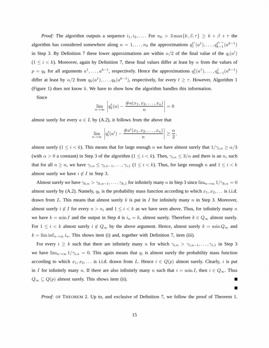
Proof: The algorithm outputs a sequencei1, i2, . . . . For n0 > 3max{k, β, τ} ≥ k + β + τ the

algorithm has considered somewhere alongn = 1, . . . , n0 the approximationsqt1

1 (a1), . . . , qt

k−1

k−1(ak−1)

in Step 3. By Definition 7 these lower approximations are within α/2 of the final value of theqi(ai)

(1 ≤ i < k). Moreover, again by Definition 7, these final values differ at least byα from the values of

p = qk for all argumentsa1, . . . , ak−1, respectively. Hence the approximationsqt1(a1), . . . , qtk−1

(ak−1)

differ at least byα/2 from qk(a1), . . . , qk(a

k−1), respectively, for everyt ≥ τ . However, Algorithm 1

(Figure 1) does not knowk. We have to show how the algorithm handles this information.

Since

limn→∞

∣

∣

∣

∣

qtk(a)−#a(x1, x2, . . . , xn)

n

∣

∣

∣

∣

= 0

almost surely for everya ∈ L by (A.2), it follows from the above that

limn→∞

∣

∣

∣

∣

qti(ai)−

#ai(x1, x2, . . . , xn)

n

∣

∣

∣

∣

≥α

2,

almost surely (1 ≤ i < k). This means that for large enoughn we have almost surely that1/γi,n ≥ α/3

(with α > 0 a constant) in Step 3 of the algorithm (1 ≤ i < k). Then,γi,n ≤ 3/α and there is anni such

that for alln ≥ ni we haveγi,n ≤ γi,n−1, . . . , γi,1 (1 ≤ i < k). Thus, for large enoughn and1 ≤ i < k

almost surely we havei 6∈ I in Step 3.

Almost surely we haveγk,n > γk,n−1, . . . , γk,1 for infinitely manyn in Step 3 sincelimn→∞ 1/γk,n = 0

almost surely by (A.2). Namely,qk is the probability mass function according to whichx1, x2, . . . is i.i.d.

drawn fromL. This means that almost surelyk is put in I for infinitely manyn in Step 3. Moreover,

almost surelyi 6∈ I for everyn > ni and1 ≤ i < k as we have seen above. Thus, for infinitely manyn

we havek = min I and the output in Step 4 isin = k, almost surely. Thereforek ∈ Q∞ almost surely.

For 1 ≤ i < k almost surelyi 6∈ Q∞ by the above argument. Hence, almost surelyk = minQ∞ and

k = lim infn→∞ in. This shows item (i) and, together with Definition 7, item (iii).

For everyi ≥ k such that there are infinitely manyn for which γi,n > γi,n−1, . . . , γi,1 in Step 3

we havelimn→∞ 1/γi,n = 0. This again means thatqi is almost surely the probability mass function

according to whichx1, x2, . . . is i.i.d. drawn fromL. Hencei ∈ Q(p) almost surely. Clearly,i is put

in I for infinitely manyn. If there are also infinitely manyn such thati = min I, then i ∈ Q∞. Thus

Q∞ ⊆ Q(p) almost surely. This shows item (ii).

Proof: OF THEOREM 2. Up to, and exclusive of Definition 7, we follow the proof of Theorem 1.

15

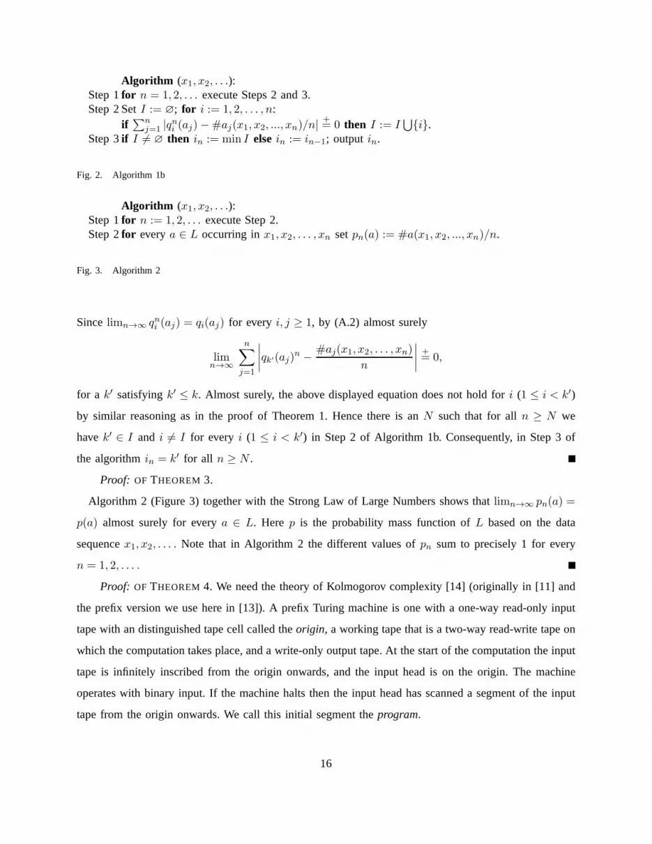
Algorithm (x1, x2, . . .):Step 1for n = 1, 2, . . . execute Steps 2 and 3.Step 2 SetI := ∅; for i := 1, 2, . . . , n:

if∑n

j=1 |qni (aj)−#aj(x1, x2, ..., xn)/n|

+= 0 then I := I

⋃

{i}.Step 3if I 6= ∅ then in := min I else in := in−1; output in.

Fig. 2. Algorithm 1b

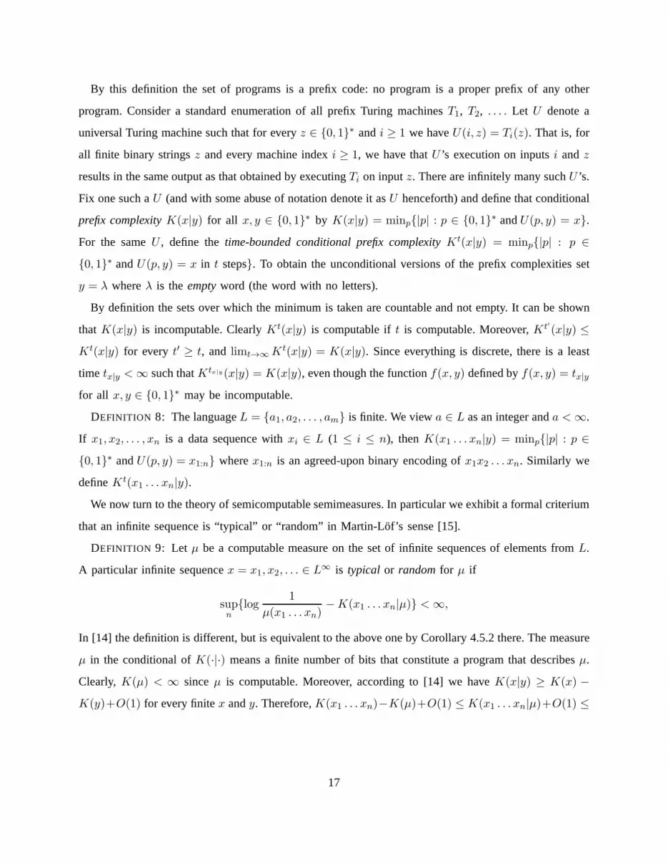
Algorithm (x1, x2, . . .):Step 1for n := 1, 2, . . . execute Step 2.Step 2for everya ∈ L occurring inx1, x2, . . . , xn setpn(a) := #a(x1, x2, ..., xn)/n.

Fig. 3. Algorithm 2

Sincelimn→∞ qni (aj) = qi(aj) for every i, j ≥ 1, by (A.2) almost surely

limn→∞

n∑

j=1

∣

∣

∣

∣

qk′(aj)n −

#aj(x1, x2, . . . , xn)

n

∣

∣

∣

∣

+= 0,

for a k′ satisfyingk′ ≤ k. Almost surely, the above displayed equation does not hold for i (1 ≤ i < k′)

by similar reasoning as in the proof of Theorem 1. Hence thereis anN such that for alln ≥ N we

havek′ ∈ I and i 6= I for every i (1 ≤ i < k′) in Step 2 of Algorithm 1b. Consequently, in Step 3 of

the algorithmin = k′ for all n ≥ N .

Proof: OF THEOREM 3.

Algorithm 2 (Figure 3) together with the Strong Law of Large Numbers shows thatlimn→∞ pn(a) =

p(a) almost surely for everya ∈ L. Here p is the probability mass function ofL based on the data

sequencex1, x2, . . . . Note that in Algorithm 2 the different values ofpn sum to precisely 1 for every

n = 1, 2, . . . .

Proof: OF THEOREM 4. We need the theory of Kolmogorov complexity [14] (originally in [11] and

the prefix version we use here in [13]). A prefix Turing machineis one with a one-way read-only input

tape with an distinguished tape cell called theorigin, a working tape that is a two-way read-write tape on

which the computation takes place, and a write-only output tape. At the start of the computation the input

tape is infinitely inscribed from the origin onwards, and theinput head is on the origin. The machine

operates with binary input. If the machine halts then the input head has scanned a segment of the input

tape from the origin onwards. We call this initial segment the program.

16

By this definition the set of programs is a prefix code: no program is a proper prefix of any other

program. Consider a standard enumeration of all prefix Turing machinesT1, T2, . . . . Let U denote a

universal Turing machine such that for everyz ∈ {0, 1}∗ andi ≥ 1 we haveU(i, z) = Ti(z). That is, for

all finite binary stringsz and every machine indexi ≥ 1, we have thatU ’s execution on inputsi andz

results in the same output as that obtained by executingTi on inputz. There are infinitely many suchU ’s.

Fix one such aU (and with some abuse of notation denote it asU henceforth) and define that conditional

prefix complexityK(x|y) for all x, y ∈ {0, 1}∗ by K(x|y) = minp{|p| : p ∈ {0, 1}∗ andU(p, y) = x}.

For the sameU , define thetime-bounded conditional prefix complexityKt(x|y) = minp{|p| : p ∈

{0, 1}∗ andU(p, y) = x in t steps}. To obtain the unconditional versions of the prefix complexities set

y = λ whereλ is theemptyword (the word with no letters).

By definition the sets over which the minimum is taken are countable and not empty. It can be shown

thatK(x|y) is incomputable. ClearlyKt(x|y) is computable ift is computable. Moreover,Kt′(x|y) ≤

Kt(x|y) for every t′ ≥ t, and limt→∞Kt(x|y) = K(x|y). Since everything is discrete, there is a least

time tx|y < ∞ such thatKtx|y(x|y) = K(x|y), even though the functionf(x, y) defined byf(x, y) = tx|y

for all x, y ∈ {0, 1}∗ may be incomputable.

DEFINITION 8: The languageL = {a1, a2, . . . , am} is finite. We viewa ∈ L as an integer anda < ∞.

If x1, x2, . . . , xn is a data sequence withxi ∈ L (1 ≤ i ≤ n), thenK(x1 . . . xn|y) = minp{|p| : p ∈

{0, 1}∗ andU(p, y) = x1:n} wherex1:n is an agreed-upon binary encoding ofx1x2 . . . xn. Similarly we

defineKt(x1 . . . xn|y).

We now turn to the theory of semicomputable semimeasures. Inparticular we exhibit a formal criterium

that an infinite sequence is “typical” or “random” in Martin-Lof’s sense [15].

DEFINITION 9: Let µ be a computable measure on the set of infinite sequences of elements fromL.

A particular infinite sequencex = x1, x2, . . . ∈ L∞ is typical or randomfor µ if

supn{log

1

µ(x1 . . . xn)−K(x1 . . . xn|µ)} < ∞,

In [14] the definition is different, but is equivalent to the above one by Corollary 4.5.2 there. The measure

µ in the conditional ofK(·|·) means a finite number of bits that constitute a program that describesµ.

Clearly, K(µ) < ∞ sinceµ is computable. Moreover, according to [14] we haveK(x|y) ≥ K(x) −

K(y)+O(1) for every finitex andy. Therefore,K(x1 . . . xn)−K(µ)+O(1) ≤ K(x1 . . . xn|µ)+O(1) ≤

17

K(x1 . . . xn) +O(1). Hence we can replace the last displayed formula by

supn{log

1

µ(x1 . . . xn)−K(x1 . . . xn)} < ∞. (A.4)

Our data is, by assumption, typical (equivalently random) for some computable measureµ. That is, the

datax1, x2, . . . satisfies (A.4) with respect toµ. We can effectively enumerate all and only semimeasures

that are semicomputable from below as the elements listed inM of (IV.2).

REMARK 6: We stress that the data is possiblyµ-random andµ′-random for different measuresµ and

µ′. In general it can be so for many measures inM. Therefore we cannot speak of the true measure, but

only of a measure for which the data is typical. ✸

To eliminate the undesirable lower semicomputable semimeasures amongµ1, µ2 . . . we sieve out the

ones that are not measures, and among the measures the ones that do not showx1, x2, . . . random to it.

To do so, we conduct for elements ofM a test for both properties. Since the test is computational we

need the (in)equality relations+

≤,+

≥,+=,

+

<,+

> of Definition 4. In particular this is needed in the properties

in Claim 3. These properties are used in Step 3 of Algorithm 3 (Figure 4).

DEFINITION 10: Since the algorithms have a round-off error, we can test only+= 0 or not

+= 0.

Consequently, we count semimeasures as measures if they satisfy (IV.1) but deviate from equalities by a

very small additive term only. More precisely,µi in the list M is counted as asemimeasure but not as

a measureif µi(z) −∑

a∈L µi(za)+> 0. If µi(z)−

∑

a∈L µi(za)+= 0 then we viewµi as ameasure.

CLAIM 2: Assume thatµi in M is a semimeasure but not a measure according to Definition 10.Then,

there is a leastz ∈ L∗ and a leastni such thatµni (z) −

∑

a∈L µni (za)

+> 0 for everyn ≥ ni.

Proof: Sinceµi is lower semicomputable and|L| < ∞, for everyz ∈ L∗ there is annz such that

for everyn ≥ nz we have

0 ≤ µi(z)− µni (z)

+= 0

and for everya ∈ L we have

0 ≤∑

a∈L

µi(za) −∑

a∈L

µni (za)

+= 0.

Therefore,

µni (z)−

∑

a∈L

µni (za)

+= µi(z) −

∑

a∈L

µi(za)+> 0. (A.5)

DEFINITION 11: Let µi be an element ofM. Assume that for alln we havei, j > 0 and i +

18

j = n. Define Zi,j,n = {z ∈ L∗ : |z| ≤ j, µni (z) −

∑

a∈L µni (za)

+

> 0} and ∆i,n = max{∆ :

Zi,j−∆,n−∆

⋂

· · ·⋂

Zi,j,n 6= ∅}.

REMARK 7: The setZi,j,n contains all stringsz ∈ L∗ of at least lengthj such thati + j = n and

µni (z) −

∑

a∈L µni (za)

+

> 0. The intersectionZi,j−∆,n−∆

⋂

· · ·⋂

Zi,j,n is the set of all stringsz of

length at leastj − ∆ that witness that the approximationsµn−∆i , . . . , µn

i are all semimesures but not

measures. The quantity∆i,n is the maximum number of approximations before and including thenth

approximation ofµi such that the samez ∈ L∗ of length at leastj −∆i,n with i+ j = n witnesses that

all these approximations are semimeasure but not measures:µn′

i (z)+>∑

a∈L µn′

i (za) for everyn′ such

thatn−∆i,n ≤ n′ ≤ n. ✸

CLAIM 3: Letµi be an element of the listM andni be as in Claim 2. Ifµi is not a measure according

to Definition 10, then for everyn ≥ ni we have∆i,n ≥ n−ni for all n ≥ ni and∆i,n = ∆i,n−1+1 for

all n > ni. If µi is a measure according to Definition 10, then for everyn there is a greatestc < ∞ such

that∆i,n < n− c andc goes to∞ with growingn. We have∆i,n < max{∆(i, n− 1), . . . ,∆(i, 1)}+1

for infinitely manyn iff µi is a measure.

Proof: If µi is not a measure then by Claim 2 there is az ∈ L∗ such thatµni (z)−

∑

a∈L µni (za)

+> 0

for all n ≥ ni. Thisz will never leave the setsZi,j,n (|z| ≤ j = n−i) for n ≥ ni. Therefore,∆i,n ≥ n−ni

and∆i,n = ∆i,n−1 + 1 for all n > ni.

If µi is a measure thenlimn→∞(µni (z) −

∑

a∈L µni (za)) = 0. Therefore, for everyz there is a least

ni,z < ∞ such thatµni (z) −

∑

a∈L µni (za)

+= 0 for all n ≥ ni,z. Hence, for everyj and everyz ∈ L∗

with |z| ≤ j we havez 6∈ Zi,j,n for all n ≥ ni,z. Thus, every finite string inZi,j,n is not a member

of Zi,j+n′−n,n′ any more for everyn′ > n. Therefore, for everyn there is a greatestc < ∞ such that

∆i,n < n− c andc goes to∞ with growingn. This implies that

∆i,n < max{∆(i, n − 1), . . . ,∆(i, 1)} + 1

for infinitely manyn. In view of the above property of semimeasures that are not measures according to

Definition 10,µi is a measure iff the last displayed equation holds.

REMARK 8: To make everything effective (computable) for Algorithm3 (Figure 4) we do not use

prefix complexity as in (A.4) but the time-bounded analog as defined. By using dovetailing, that is,

n = 1, 2, . . . with all combinations ofi, j > 0 such thati + j = n and n is the number of steps, as

in Definition 11, with growingn everyµni (z) with |z| ≤ j for every particulari, j, n is computed and

considered.

19

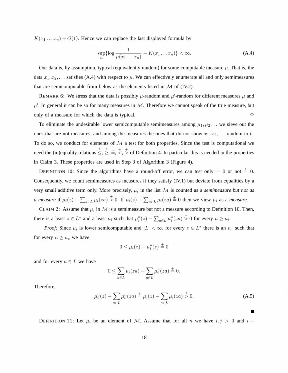
In Algorithm 3 one wants to determine the indexesi of elementsµi in the list M such thatµi is a

measure. This happens in Steps 2 and 3 as follows. For growingn the fact that indexi is selected to

go in I means thatµi is possibly a measure. Eventually, ifn is large anough this possibility will turn

into a certainty. Moreover, this will hold for every measureµi. Thus, for everyi with growing n, but

not computably, it is decided thatµi is a measure or not. If it is a measure, then it keeps on figuringin

the second part of the algorithm, if it is decided not to be a measure then it will not figure in the second

part of the algorithm.

This second part of the algorithm determines for which measures the datax1, x2, . . . is random. Note

that this part initially also may consider nonmeasures. Butwith growing n, because of the first part of

the algorithm, for every indexi it will consider only measures but not nonmeasuresµi. If for some

n the index i is selected then in Step 5 the algorithm computes then-approximationsρ(i, j′, n) :=

log 1/µni (x1 . . . xj′)−Kn(x1 . . . xj′) (1 ≤ j′ ≤ j, j = n− i). This in order to obtain approximations to

the elements constituting the initial segment of the sequence of which equation (A.4) takes the supremum.

In Step 6 the algorithm takes the maximumσ(i, n, j′) := max{ρ(i, j′′, n) : 1 ≤ j′′ ≤ j′} over the initial

segments of this initial segment. In Step 7 it determines foreveryµi concerned how long the longest flat

plateau of this sequence of maxima is.

Supposeµi is a measure for whichx1, x2, . . . is random. If there exists an0 such that then0-

approximation ofρ(i, j0, n0) has reached the supremum in (A.4), then for everyj ≥ j0 and n ≥ n0

we have thatρ(i, j, n) reaches this supremum. (Reaching means “is within a unit.”)To select aµi one

looks for theρ(i, ·, ·) that gives the longest flat plateau, that is, has reached the supremum in (A.4) the

soonest in terms of the initial segment ofx1, x2, . . . . Thus, in Step 7 the algorithm compares the length

of the flat plateau with the top score, and changes the latter if it is exceeded. In Step 8 the algorithm

either selects the index resulting in a new or equal top scoreor goes with the index of approximation

n− 1. Note that with growingn nonmeasures are excluded in the first part of the algorithm. Thus, with

growingn, the measureµi that reaches (A.4) soonest and has the longest flat plateau, has an indexi that

is not (eventually) excluded by the first part of the algorithm. ✸

DEFINITION 12: Letµi in list M be a measure according to Definition 10 andx1, x2, . . . be an infinite

sequence of elements fromL. By (A.4) we haveµi ∈ M(x) iff there is aσi < ∞ such that

σi = maxj

{⌊

log1

µi(x1 . . . xj)−K(x1 . . . xj)

⌋

− 1

}

(A.6)

for 1 ≤ j ≤ ∞. Definemi as the leastj for which σi is reached.

20

Algorithm (x1, x2, . . .):Step 1m := 0; for n = 1, 2, . . . execute Steps 2 through 8.Step 2I := ∅; for every i, j > 0 satisfying i + j = n, compute∆i,n (note j = n − i) and execute

Steps 3 through 7.Step 3if ∆i,n < max{∆(i, n− 1), . . . ,∆(i, 1)}+1 then I := I

⋃

{i} (by Claim 3,i ∈ I for infinitelymanyn iff µi is a measure).

Step 4if I 6= ∅ then execute Steps 5 through 7 for everyi ∈ I.Step 5for j′ := 1, . . . , j setρ(i, j′, n) := log 1/µn

i (x1 . . . xj′)−Kn(x1 . . . xj′).Step 6for j′ := 1, . . . , j setσ(i, n, j′) := max{ρ(i, j′′, n) : 1 ≤ j′′ ≤ j′}.Step 7s(i, n) := max{s : ⌊σ(i, n, r)⌋ − 1 = · · · = ⌊σ(i, n, r + s)⌋ − 1, 1 ≤ r ≤ r + s ≤ j}; if

s(i, n) ≤ m then I := ∅ else m := s(i, n).Step 8if I 6= ∅ then in := min{i : s(i, n) = m} else in := in−1; output in.

Fig. 4. Algorithm 3

REMARK 9: In Definition 12 we have replaced “measure” by “measure according to Definition 10.”

We have replaced the “sup” in (A.4) by “max” by rounding down. Moreover, by rounding down and

subtracting 1 we have taken care thatmi < ∞. ✸

(Proof of the theorem continued.) The sequence of outputs ofAlgorithm 3 are indexesi1, i2, . . . of

lower semicomputable semimeasures inM, such that possiblyij < ij+1, ij > ij+1, or ij = ij+1. By

Claim 3, for every measure (Definition 10)µi in M we havei ∈ I in Step 3 of the algorithm for

infinitely manyn. For large enoughn index i /∈ I of a nonmeasureµi. So for every indexi there is a

large anoughn such thati ∈ I only if µi is a measure. These measures are treated in Steps 4 through 8.

By assumption the datax = x1, x2, . . . is random (typical) for some measure inM. Let this be measure

µk.

Let us look at long plateauss(i, n) for measuresµi such that eitherx = x1, x2, . . . is not random to

it or mi > n (with mi as in Definition 12). For a measureµi such thatx = x1, x2, . . . is not random to

it, s(i, n) can be any constantc. However the lefthand side of (A.4) goes to infinity in this case, so we

know thats(i, n′) = 1 for somen′ ≥ n. Since the datax = x1, x2, . . . is random toµk, for all n that are

large enoughs(k, n) = s(k, n−1)+1 by Claim 3. Hence, for large enoughn we haves(k, n) > s(i, n),

sinces(k, n) → ∞ with n → ∞. For a measureµj with j 6= k such thatx = x1, x2, . . . is random to it,

s(j, n) can be a constantc < σj while n < mj . That is, the maximum in (A.6) has not yet been reached.

Again we know thats(j, n′) = 1 for somen′ > n. Hence without loss of generality we can exclude

cases like measuresµi andµj. Let us consider only measuresµl and stepsn, such thatx = x1, x2, . . .

is random toµl andn ≥ ml.

21

Without loss of generality we can assume that we computes(i, n) for every measureµi in M and

everyn according to Steps 6 and 7, and not just wheni ∈ I. In particular we can do so forµk. By

Claim 3, for everyn that is large enough we haves(k, n) ≤ s(i, k−1)+1 ands(k, n) = s(k, n−1)+1.

Let i satisfymk < i. Then,s(i,mk) = 0 (the set over whichs(i,mk) is maximized in Step 7 equals

∅). Sinces(i, n) ≤ s(i, n) + 1 for all n, we haves(i, n) < s(k, n) ≤ m (with m as in Step 7) for all

n ≥ mk. Hencein 6= i in Step 8 ifn is large enough. LetA be the set of measuresµi with i < mk.

Then |A| < mk andM∞ ⊆ A. Hence|M∞| < mk < ∞.

Since|M∞| < mk, and by Steps 5,6,7 the output of Algorithm 3 is an infinite sequencei1, i2, . . . , we

have that somei0 < mk occurs infinitely often in this sequence. HenceM∞ 6= ∅.

Let the indexi of a measureµi occur inM∞. Thens(i, n) is larger thanm in Step 7 for infinitely

manyn. (It is impossible thatin = in−1 for an infinitely long run ofn’s sincem → ∞ with n → ∞.

The latter statement is a consequence ofs(k, n) growing with n.) Sincem → ∞ with n → ∞ we have

s(i, n) → ∞ with n → ∞. By the definition ofs(·, ·) and (A.6), the datax = x1, x2, . . . is random with

respect to the measureµi. Hence,M∞ ⊆ M(x). This proves the theorem.

REFERENCES

[1] D. Angluin, Identifying languages from stochastic examples, Yale University, Dept. of Computer Science, Technical report,

New Haven, Conn., USA, 1988.

[2] S.B. Cooper, P. Odifreddi (2003). Incomputability in nature, Pp. 137–160 in S. B. Cooper and S. S. Goncharov, Eds.,

Computability and Models: Perspectives East and West, Plenum, New York, 2003.

[3] T.M. Cover and J.A. Thomas,Elements of Information Theory, Wiley, New York, 1991.

[4] E.M. Gold, Limiting recursion,J. Symb. Logic, 30(1965), 28-48.

[5] E.M. Gold, Language identification in the limit,Inform. Contr., 10(1967), 447–474.

[6] W. Feller, An Introduction to Probability Theory and Its Applications, Vol. 1, Wiley, New York, 1968 (third edition).

[7] A. Hsu, N. Chater and P.M.B. Vitanyi, The probabilisticanalysis of language acquisition: Theoretical, computational, and

experimental analysis,Cognition,120(2011), 380–390.

[8] S. Jain, D.N. Osherson, J.S. Royer, A. Sharma,Systems that Learn, MIT Press, Cambridge, Mass., 1999 (second edition).

[9] A.N. Kolmogorov, Grundbegriffe der Wahrscheinlichkeitsrechnung, Springer-Verlag, Berlin, 1933.

[10] A.N. Kolmogorov, Sur la loi forte des grandes nombres,C. r. Acad. Sci. Paris, 191(1930), 910–912. See also A.N.

Kolmogorov, Grundbegriffe der Wahrscheinlichkeitsrechnung, Springer-Verlag, Berlin, 1933. See also F.P. Cantelli, Sulla

probabilita come limite della frequenza,Rendiconti della R. Academia dei Lincei, Classe di scienze fisische matematiche

e naturale, Serie5a, 26(1917), 39–45.

[11] A.N. Kolmogorov, Three approaches to the quantitativedefinition of information, Problems Inform. Transmission,

1:1(1965),1–7.

[12] M. Kracht, The Mathematics of Language, Mouton & de Gruyter, Berlin, 2003.

22

[13] L.A. Levin, Laws of information conservation (non-growth) and aspects of the foundation of probability theory,Problems

Inform. Transmission, 10(1974), 206–210.

[14] M. Li and P.M.B. Vitanyi,An Introduction to Kolmogorov Complexity and Its Applications, Springer-Verlag, New York,

2008 (third edition).

[15] P. Martin-Lof, The definition of random sequences,Inform. Control, 9:6(1966), 602–619.

[16] S. Pinker, Formal models of language learning,Cognition7(1979), 217–283.

[17] K.R. Popper,The Logic of Scientific Discovery, Hutchinson, London, 1959.

[18] Z.W. Pylyshyn, Z. W.,Computation and Cognition, MIT Press, Cambridge, Mass., 1984.

[19] F. Rieke, D. Warland, R. de Ruyter van Steveninck, W. Bialek, (1997).Spikes: Exploring the Neural Code, MIT Press,

Cambridge, Mass., 1997.

[20] A.M. Turing, On computable numbers, with an application to the Entscheidungsproblem,Proc. London Mathematical

Society2, 42(1936), 230–265, ”Correction”, 43(1937), 544–546.

[21] A.K. Zvonkin and L.A. Levin, The complexity of finite objects and the development of the concepts of information and

randomness by means of the theory of algorithms,Russian Math. Surveys, 25:6(1070), 83–124.

23