-1

Connectivity, probabilities and persistence:

comparing reserve selection strategies

ASTRID J.A. VAN TEEFFELEN*, MAR CABEZA andATTE MOILANENMetapopulation Research Group, Department of Biological & Environmental Sciences, University of

Helsinki, P.O. Box 65, Viikinkaari 1, FIN-00014, Finland; *Author for correspondence (e-mail:

astrid.vanteeffelen@helsinki.fi; phone: +358-9-191-57913; fax: +358-9-191-57694)

Received 13 January 2004; accepted in revised form 19 August 2004

Key words: Connectivity, Habitat loss, Habitat model, Persistence, Probability of occurrence,

Reserve selection

Abstract. Reserve selection methods are often based on information on species’ occurrence. This

can be presence–absence data, or probabilities of occurrence estimated with species distribution

models. However, the effect of the choice of distribution model on the outcome of a reserve

selection method has been ignored. Here we test a range of species distribution models with three

different reserve selection methods. The distribution models had different combinations of variables

related to habitat quality and connectivity (which incorporates the effect of spatial habitat con-

figuration on species occurrence). The reserve selection methods included (i) a minimum set ap-

proach without spatial considerations; (ii) a clustering reserve selection method; and (iii) a dynamic

approach where probabilities of occurrence are re-evaluated according to the spatial pattern of

selected sites. The sets of selected reserves were assessed by re-computing species probability of

occurrence in reserves using the best probability model and assuming loss of non-selected habitat.

The results show that particular choices of distribution model and selection method may lead to

reserves that overestimate the achieved target; in other words, species may seem to be represented

but the reserve network may actually not be able to support them in the long-term. Instead, the use

of models that incorporated connectivity as a variable resulted in the selection of aggregated

reserves with higher potential for species long-term persistence. As reserve design aims at the long-

term protection of species, it is important to be aware of the uncertainties related to model and

method choice and their implications.

Introduction

During the past 20 years a range of systematic quantitative methods, oftencalled site selection algorithms, has been developed for the selection of reservenetworks for biodiversity conservation based on empirical data (Kirkpatrick1983; Pressey et al. 1993; Csuti et al. 1997; Williams 1998; Cabeza andMoilanen 2001; Margules et al. 2002). Earliest reserve selection formulationsaimed at identifying sets of sites that together represent each species (a givennumber of times) with minimum cost (minimum set proportional coverageproblem) (Margules et al. 1988; Csuti et al. 1997; Howard et al. 1998). Becauseminimum set coverage approaches were applied to static snapshots of presence/absence data, they implicitly assumed that a species which is present at site i at

Biodiversity and Conservation (2006) 15:899–919 � Springer 2006

DOI 10.1007/s10531-004-2933-8

the time of the survey, will persist there indefinitely. Subsequently, severalstudies have demonstrated that one (or a few) representation per species in areserve network does not ensure the long-term persistence of the species(Margules et al. 1994; Virolainen et al. 1999; Rodrigues et al. 2000; Cabeza andMoilanen 2001). One fundamental reason for this is spatial populationdynamics, which causes species turnover in sites, including the reserve sites.Consequently, the need to incorporate spatial population dynamics into siteselection procedures has been emphasised (Nicholls 1998; Hanski 1999; Cabezaand Moilanen 2001; Verboom et al. 2001).

Several methods have been suggested for the incorporation of spatial pop-ulation dynamics into reserve selection. One way is the inclusion of a meta-population model which explicitly takes species-specific spatial dynamics intoaccount (Moilanen and Cabeza 2002). A major drawback of this method is thelarge amount of data necessary for parameterising the model for each species.Several authors have suggested qualitative clustering of reserves to reducenegative effects of fragmentation (Nicholls and Margules 1993; Heijnis et al.1999; Possingham et al. 2000; Cabeza et al. 2004a). Connectivity measures havebeen applied in reserve selection by few authors, who have noted the connec-tion to population persistence. Most commonly non-species-specific measures,such as nearest neighbour- and buffer measures (Araujo et al. 2002; buffermeasure and Briers 2002; distance-dependant connectivity), have been used.(Van Langevelde et al. 2000) have accounted for species-specific dispersalcapacity when applying reserve selection for a single species, by the selection ofsites within dispersal distance to existing reserves. Since reserve network designtypically concerns conservation planning for multiple species, which each mayexperience a reserve network differently from a spatial perspective, it is highlyrecommended to use species-specific measures of connectivity (Hanski 1994;Schumaker 1996; With et al. 1997; Van Langevelde 2000; D’Eon et al. 2002;Moilanen and Nieminen 2002). To our knowledge, only Ferrier et al. (2002)and Cabeza (2003) have applied species-specific parameters to evaluateconnectivity of the landscape in the context of multiple-species reserve design.

Reserve selection exercises have often been based on presence–absence (orpresence-only) information on the features to be protected. Simple reserveselection methods based on presence (-absence) data may however fail to selectthe sites where species have higher probabilities of persistence (Araujo andWilliams 2000 and references therein). One alternative to presence–absence dataare probabilities of occurrence (Austin et al. 1984; Margules and Stein 1989;Williams and Araujo 2002; Cabeza 2003; Cabeza et al. 2004a). Probabilities ofoccurrence indicate the likelihood that a species is present at a certain site, whichcan be influenced by different species-dependent factors such as habitatrequirements, species’ population dynamics and vulnerability to threats (Araujoand Williams 2000; Williams and Araujo 2000). An advantage is that proba-bilities can be modelled and estimated using a standard statistical method (e.g.logistic regression, which is a standard technique in this context; Austin et al.1984; Ter Braak and Looman 1986; Pearce and Ferrier 2000). Probabilities

900

can be used to evaluate different reserve compositions and effects of land usechange or other threats. The use of (species-specific) connectivity measures inpredictive models facilitates the evaluation of reserve composition and land-scape change, as probabilities do not only depend on local environmentalinformation, but also on information form the neighbourhood. In habitatmodelling literature similar contextual variables (variables that reflect envi-ronmental information within a certain radius around a site) are frequentlyapplied (Grashof-Bokdam 1997; Osborne et al. 2001; Ferrier et al. 2002). In thisstudy we use different probability models, with and without (species-specific)connectivity measures, to provide probabilities as input for several reserveselection methods.

The type of information that is used as the basis for reserve selection is likelyto affect the final reserve network in terms of location, shape and size. Forexample, a model that uses only local habitat information will predict higherprobabilities of occurrence in sites with high-quality habitat, irrespective oftheir location. If connectivity measures are also included in the model, higherprobabilities might only occur in good-quality sites that are near other good-quality sites. A reserve selection algorithm evaluates a reserve network solutionwith a particular model for each species during optimisation. Once the solutionsatisfies the criteria (e.g. it has found the smallest set of sites that representseach species at least n times), the algorithm finishes. However, when thatparticular solution is evaluated using another model, the representation of thespecies in the reserve network might not meet the required target level. Thisissue is usually ignored in reserve selection, as typical reserve selection studiesare based on one set of probabilities arising from one model only. We dem-onstrate the differences that can occur in the expected number of occurrencesof each species in a reserve network, due to model choice. As the expectednumber of occurrences is related to the persistence of the species in the net-work, it is of major importance to be aware of the uncertainties related tomodel choice in reserve selection.

Cabeza (2003) and Cabeza et al. (2004a) combine probabilities of occurrencewith spatial reserve design. A novel feature of these two studies is that theyacknowledge that habitat loss or degradation outside the reserve network mightnegatively influence probabilities of occurrence within reserve sites (Gastonet al. 2002; Cabeza and Moilanen 2003). In other words, the probabilities ofoccurrence in selected (reserved) sites depend on the quality and spatial patternof both reserved and unreserved sites. Several authors (Possingham et al. 2000;Nalle et al. 2002; Cabeza et al. 2004a, b) attempt to minimize negative externaleffects by aiming at the selection of aggregated reserves, by means of a penaltyfor boundary length. Alternatively, Cabeza (2003) makes probabilities ofoccurrence depend explicitly on habitat information and connectivity of theselected sites only. It is important to note that connectivity here is a measurethat incorporates a species-specific parameter, which scales the effect of distanceon migration success. Consequently, the pattern of selected sites will affectprobabilities of occurrence within reserve sites in a species-specific way, which is

901

accounted for during reserve selection with the dynamic probability approach(Cabeza 2003).

The aim of this paper is to point out that the choice for a probability modelas basis for reserve selection can make a substantial difference to the compo-sition and size of a reserve network. This effect becomes even stronger whenprobabilities of occurrence depend on the presence of potential source popu-lations in the neighbourhood as well, through the use of connectivity measuresand assuming loss of unprotected habitat. Here, such effects are assessed bycomparing solutions from three reserve selection strategies in terms of theexpected number of occurrences they ensure for each species. The data used forcomparing the three strategies are data sets from seven bird species from theNetherlands, and habitat maps, with which their occurrence is modelled.

Material and methods

Study system and data

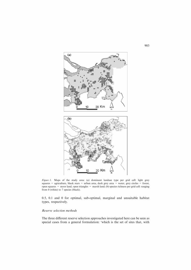
The study area (�1850 km2) is the west part of the province Noord-Brabant,the Netherlands (51�39¢ N, 4�40¢ E). The area is bordered by the river Meuse tothe north, closed sea-areas and land to the west and by land to the east andsouth. The landscape in this area is diverse: The larger part of the regionconsists of agricultural habitat, in the north and west marshlands are presentand in the southern part forest and moorland are more abundant (Figure 1(a)).There are a few cities along the horizontal axis of the area.

Data on seven bird species was used for the comparison of different siteselection strategies (Table 1). Atlas information on presence/absence as well asthe number of breeding pairs was surveyed per grid cell (1000 m · 1000 m)between 1989 and 1997 (Vogelonderzoek Nederland SOVON, 2002, data fromSamenwerkingsverband Westbrabantse Vogelwerkgroepen (SWEV) andProvince of Noord-Brabant). Birds were chosen, since barriers in the landscape(such as roads) have less affect on their dispersal than on dispersal of grounddwelling species. Consequently it was possible to model occurrences of birdswithout explicit consideration of these barriers. The selected species have dif-ferent habitat requirements (although partially overlapping); therefore the re-serve network needs to cover different habitat types. Figure 1(b) shows thespecies richness in the study area, from which it is not obvious which sitesshould be protected if one wants to protect these species in an efficient andeffective manner.

The habitat data consists of 96 habitat types, including all (semi-)naturaland agricultural features, in hectares per grid cell (250 m · 250 m) (Pouwelset al. 2002). Since the species data is available per 1 km2 grid cells, habitatdata was transformed to 1 km2 grid cells by summation. Pouwels et al. (2002)also described habitat suitability indices for several species (see Reijnen et al.2001 for methods), including those used here. These indices have values 1.0,

902

0.5, 0.1 and 0 for optimal, sub-optimal, marginal and unsuitable habitattypes, respectively.

Reserve selection methods

The three different reserve selection approaches investigated here can be seen asspecial cases from a general formulation: ‘which is the set of sites that, with

Figure 1. Maps of the study area: (a) dominant landuse type per grid cell: light grey

squares = agriculture, black stars = urban area, dark grey area = water, grey circles = forest,

open squares = moor land, open triangles = marsh land; (b) species richness per grid cell: ranging

from 0 (white) to 7 species (black).

903

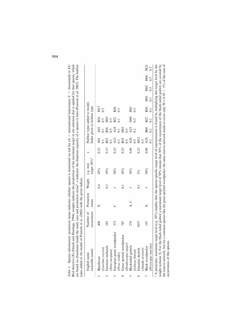
Table

1.

Speciesinform

ation:protectionstatusindicateswhether

speciesismentioned

onredlist

(A=

internationalim

portance;C

=threatened)orEU

Birddirective(X

)(O

sieckandHustings,1994);weights

indicate

theproportionofthemaxim

um

target

insite

selectionthatisapplied

forthatspecies,which

are

basedonabundance

insidethestudyareaandprotectionstatusa.aindicatesthedispersalcapacity

ofaspecies(1/km)(Pouwelset

al.2002).Thehabitat

types

added

tothemodel

ofPouwelset

al.(2002)withthegiven

indices.

English

name

(scientificname)

Number

of

occurrences

Protection

status

Weight

e.g.max

target

50%

aa

Habitattypes

added

tomodel.

Index

given

tohabitattype

1Bluethroat

406

X0.4

20%

0.23

A01

A03

B24

M17

(Luscinia

svecica)

0.1

0.1

0.5

0.5

2Eurasiannuthatch

185

0.2

10%

0.15

B22

B26

H03

(Sitta

europaea)

0.1

0.5

0.5

3Europeangreen

woodpecker

373

C1

50%

0.23

A23

A24

B22

B26

(Picusviridis)

0.1

0.1

0.1

0.5

4Greatspotted

woodpecker

747

0.1

50%

0.23

B14

H03

(Dendrocopusmajor)

0.5

0.5

5Blacktailed

godwit

279

A,C

150%

0.08

A20

A23

D08

H01

(Lim

osa

limosa)

0.5

0.1

0.5

0.5

6Eurasianskylark

1037

0.1

5%

0.23

M12

(Alaudaarvensis)

0.5

7Black

woodpecker

197

X1

50%

0.08

A24

B04

B22

B26

H01

H02

H06

M21

(Dryocopusmartius)

0.1

0.1

0.1

0.1

0.1

0.5

0.5

0.5

aA

particular,maxim

um

target

level

(e.g.50%)im

plies

thatthespecies-specifictarget

level

ofrepresentationisfoundbymultiplyingthistarget

level

bythe

weight(column5).Fortheblack-tailed

godwitamaxim

um

target

levelof50%

meansthat50%

oftheoccurrencesoftheblack-tailed

godwitare

covered

by

thereservenetwork,butforacommonspecieslikethegreatspotted

woodpecker

thesamereservenetwork

needsto

cover

only

50

·0.10=

5%

ofthesum

of

occurrencesofthisspecies.

904

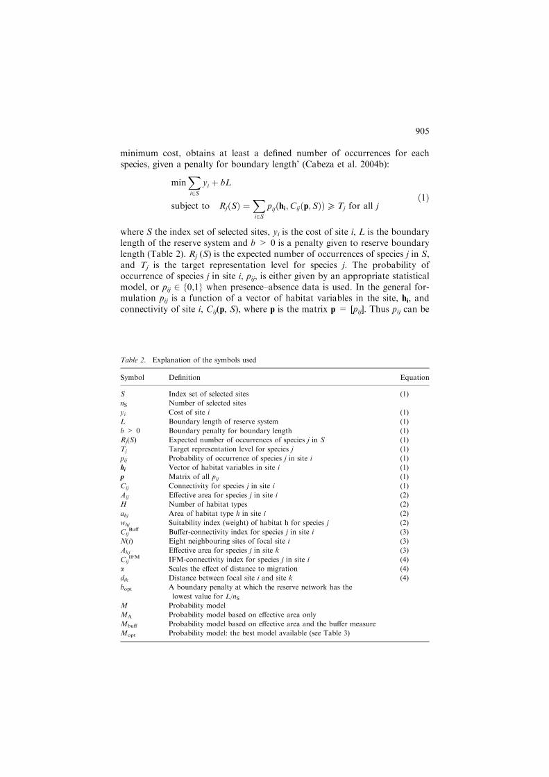
minimum cost, obtains at least a defined number of occurrences for eachspecies, given a penalty for boundary length’ (Cabeza et al. 2004b):

minX

i2Syi þ bL

subject to RjðSÞ ¼X

i2Spijðhi;Cijðp;SÞÞPTj for all j

ð1Þ

where S the index set of selected sites, yi is the cost of site i, L is the boundarylength of the reserve system and b > 0 is a penalty given to reserve boundarylength (Table 2). Rj (S) is the expected number of occurrences of species j in S,and Tj is the target representation level for species j. The probability ofoccurrence of species j in site i, pij, is either given by an appropriate statisticalmodel, or pij 2 {0,1} when presence–absence data is used. In the general for-mulation pij is a function of a vector of habitat variables in the site, hi, andconnectivity of site i, Cij(p, S), where p is the matrix p = [pij]. Thus pij can be

Table 2. Explanation of the symbols used

Symbol Definition Equation

S Index set of selected sites (1)

nS Number of selected sites

yi Cost of site i (1)

L Boundary length of reserve system (1)

b > 0 Boundary penalty for boundary length (1)

Rj(S) Expected number of occurrences of species j in S (1)

Tj Target representation level for species j (1)

pij Probability of occurrence of species j in site i (1)

hi Vector of habitat variables in site i (1)

p Matrix of all pij (1)

Cij Connectivity for species j in site i (1)

Aij Effective area for species j in site i (2)

H Number of habitat types (2)

ahj Area of habitat type h in site i (2)

whj Suitability index (weight) of habitat h for species j (2)

CijBuff Buffer-connectivity index for species j in site i (3)

N(i) Eight neighbouring sites of focal site i (3)

Akj Effective area for species j in site k (3)

CijIFM IFM-connectivity index for species j in site i (4)

a Scales the effect of distance to migration (4)

dik Distance between focal site i and site k (4)

bopt A boundary penalty at which the reserve network has the

lowest value for L/nSM Probability model

MA Probability model based on effective area only

Mbuff Probability model based on effective area and the buffer measure

Mopt Probability model: the best model available (see Table 3)

905

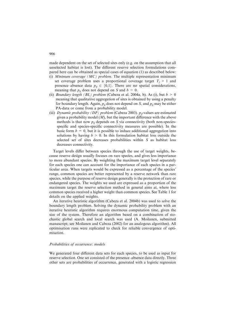
made dependent on the set of selected sites only (e.g. on the assumption that allunselected habitat is lost). The different reserve selection formulations com-pared here can be obtained as special cases of equation (1) as described below:(i) Minimum coverage (MC) problem. The multiple representation minimum

set coverage problem uses a proportional coverage target Tj > 1 andpresence–absence data pij 2 {0,1}. There are no spatial considerations,meaning that pij does not depend on S and b = 0.

(ii) Boundary length (BL) problem (Cabeza et al. 2004a, b). As (i), but b > 0meaning that qualitative aggregation of sites is obtained by using a penaltyfor boundary length. Again, pij does not depend on S, and pij may be eitherPA-data or come from a probability model.

(iii) Dynamic probability (DP) problem (Cabeza 2003). pij-values are estimatedgiven a probability model (M), but the important difference with the abovemethods is that now pij depends on S via connectivity (both non-species-specific and species-specific connectivity measures are possible). In thebasic form b = 0, but it is possible to induce additional aggregation intosolutions by having b > 0. In this formulation habitat loss outside theselected set of sites decreases probabilities within S as habitat lossdecreases connectivity.

Target levels differ between species through the use of target weights, be-cause reserve design usually focuses on rare species, and gives less importanceto more abundant species. By weighting the maximum target level separatelyfor each species one can account for the importance of each species in a par-ticular area. When targets would be expressed as a percentage of the species’range, common species are better represented by a reserve network than rarespecies, while the purpose of reserve design generally is the protection of rare orendangered species. The weights we used are expressed as a proportion of themaximum target the reserve selection method in general aims at, where lesscommon species received a higher weight than common species. See Table 1 fordetails on the applied weights.

An iterative heuristic algorithm (Cabeza et al. 2004b) was used to solve theboundary length problem. Solving the dynamic probability problem with aniterative heuristic algorithm requires enormous computation time, given thesize of the system. Therefore an algorithm based on a combination of sto-chastic global search and local search was used (A. Moilanen, submittedmanuscript; see Moilanen and Cabeza (2002) for an analogous algorithm). Alloptimisation runs were replicated to check for reliable convergence of opti-misation.

Probabilities of occurrence: models

We generated four different data sets for each species, to be used as input forreserve selection. One set consisted of the presence–absence data directly. Threeother sets are probabilities of occurrence, generated with a logistic regression

906

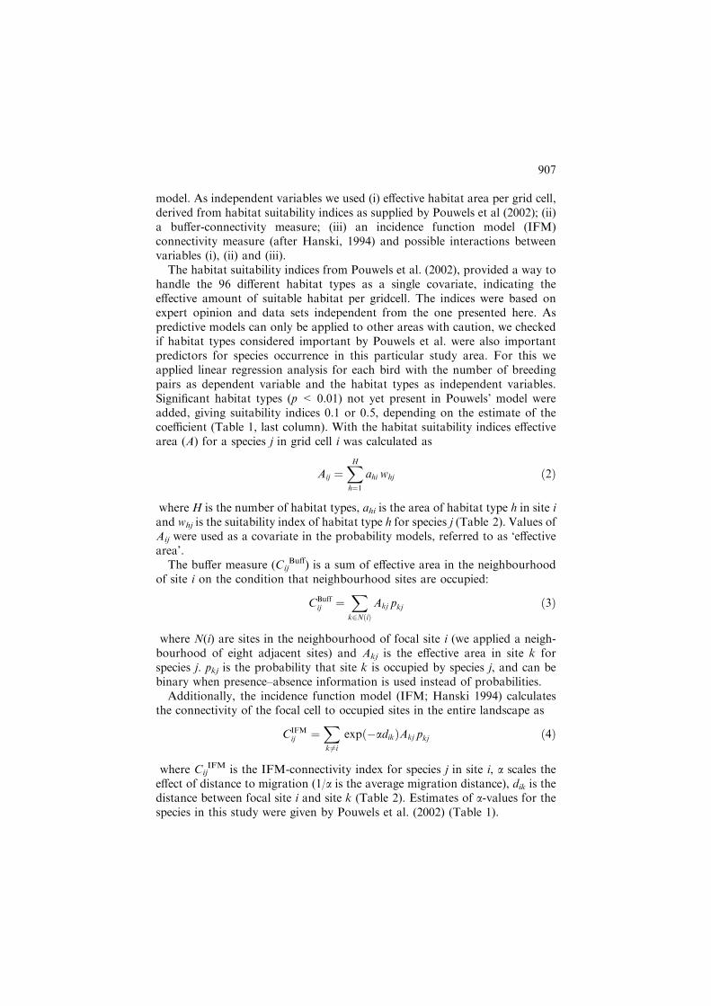
model. As independent variables we used (i) effective habitat area per grid cell,derived from habitat suitability indices as supplied by Pouwels et al (2002); (ii)a buffer-connectivity measure; (iii) an incidence function model (IFM)connectivity measure (after Hanski, 1994) and possible interactions betweenvariables (i), (ii) and (iii).

The habitat suitability indices from Pouwels et al. (2002), provided a way tohandle the 96 different habitat types as a single covariate, indicating theeffective amount of suitable habitat per gridcell. The indices were based onexpert opinion and data sets independent from the one presented here. Aspredictive models can only be applied to other areas with caution, we checkedif habitat types considered important by Pouwels et al. were also importantpredictors for species occurrence in this particular study area. For this weapplied linear regression analysis for each bird with the number of breedingpairs as dependent variable and the habitat types as independent variables.Significant habitat types (p < 0.01) not yet present in Pouwels’ model wereadded, giving suitability indices 0.1 or 0.5, depending on the estimate of thecoefficient (Table 1, last column). With the habitat suitability indices effectivearea (A) for a species j in grid cell i was calculated as

Aij ¼XH

h¼1ahi whj ð2Þ

where H is the number of habitat types, ahi is the area of habitat type h in site iand whj is the suitability index of habitat type h for species j (Table 2). Values ofAij were used as a covariate in the probability models, referred to as ‘effectivearea’.

The buffer measure (CijBuff) is a sum of effective area in the neighbourhood

of site i on the condition that neighbourhood sites are occupied:

CBuffij ¼

X

k2NðiÞAkj pkj ð3Þ

where N(i) are sites in the neighbourhood of focal site i (we applied a neigh-bourhood of eight adjacent sites) and Akj is the effective area in site k forspecies j. pkj is the probability that site k is occupied by species j, and can bebinary when presence–absence information is used instead of probabilities.

Additionally, the incidence function model (IFM; Hanski 1994) calculatesthe connectivity of the focal cell to occupied sites in the entire landscape as

CIFMij ¼

X

k 6¼iexpð�adikÞAkj pkj ð4Þ

where CijIFM is the IFM-connectivity index for species j in site i, a scales the

effect of distance to migration (1/a is the average migration distance), dik is thedistance between focal site i and site k (Table 2). Estimates of a-values for thespecies in this study were given by Pouwels et al. (2002) (Table 1).

907

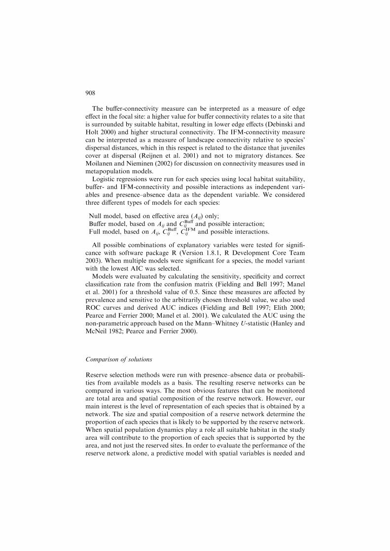
The buffer-connectivity measure can be interpreted as a measure of edgeeffect in the focal site: a higher value for buffer connectivity relates to a site thatis surrounded by suitable habitat, resulting in lower edge effects (Debinski andHolt 2000) and higher structural connectivity. The IFM-connectivity measurecan be interpreted as a measure of landscape connectivity relative to species’dispersal distances, which in this respect is related to the distance that juvenilescover at dispersal (Reijnen et al. 2001) and not to migratory distances. SeeMoilanen and Nieminen (2002) for discussion on connectivity measures used inmetapopulation models.

Logistic regressions were run for each species using local habitat suitability,buffer- and IFM-connectivity and possible interactions as independent vari-ables and presence–absence data as the dependent variable. We consideredthree different types of models for each species:

Null model, based on effective area (Aij) only;Buffer model, based on Aij and Cij

Buff and possible interaction;Full model, based on Aij, Cij

Buff, CijIFM and possible interactions.

All possible combinations of explanatory variables were tested for signifi-cance with software package R (Version 1.8.1, R Development Core Team2003). When multiple models were significant for a species, the model variantwith the lowest AIC was selected.

Models were evaluated by calculating the sensitivity, specificity and correctclassification rate from the confusion matrix (Fielding and Bell 1997; Manelet al. 2001) for a threshold value of 0.5. Since these measures are affected byprevalence and sensitive to the arbitrarily chosen threshold value, we also usedROC curves and derived AUC indices (Fielding and Bell 1997; Elith 2000;Pearce and Ferrier 2000; Manel et al. 2001). We calculated the AUC using thenon-parametric approach based on the Mann–Whitney U-statistic (Hanley andMcNeil 1982; Pearce and Ferrier 2000).

Comparison of solutions

Reserve selection methods were run with presence–absence data or probabili-ties from available models as a basis. The resulting reserve networks can becompared in various ways. The most obvious features that can be monitoredare total area and spatial composition of the reserve network. However, ourmain interest is the level of representation of each species that is obtained by anetwork. The size and spatial composition of a reserve network determine theproportion of each species that is likely to be supported by the reserve network.When spatial population dynamics play a role all suitable habitat in the studyarea will contribute to the proportion of each species that is supported by thearea, and not just the reserved sites. In order to evaluate the performance of thereserve network alone, a predictive model with spatial variables is needed and

908

is here represented by the best models (Mopt). Following, all solutions areevaluated with this model, while probabilities are only based on the reservesites only (in other words: unprotected habitat is assumed to be lost). Wecompared reserve networks in two ways: (1) evaluation of the reserve networksproduced by different methods and with different models, but all aiming at thesame target level of representation. As these solutions are likely to differ in areaand spatial composition, they will differ in terms of the expected number ofoccurrences they support. As larger reserves evidently protect a higher pro-portion of each species, comparison; (2) concerns the evaluation of reservenetworks from different methods and with different models, but with a com-parable area. If differences occur in performance of these networks (expressedas the expected number of occurrences), it is no longer an effect from thereserve area, but more likely from the reserve’s spatial composition.

Results

Predicting species occurrence

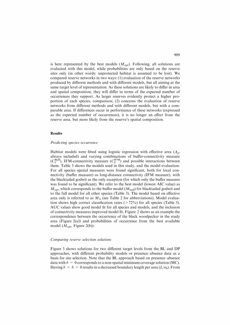
Habitat models were fitted using logistic regression with effective area (Aij,always included) and varying combinations of buffer-connectivity measure(Cij

Buff), IFM-connectivity measure (CijIFM) and possible interactions between

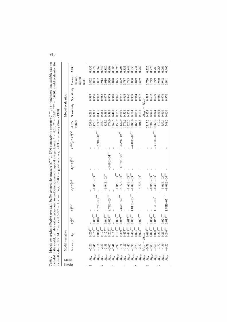
them. Table 3 shows the models used in this study, and the model evaluation.For all species spatial measures were found significant, both for local con-nectivity (buffer measure) as long-distance connectivity (IFM measure), withthe blacktailed godwit as the only exception (for which only the buffer measurewas found to be significant). We refer to the best model (lowest AIC value) asMopt, which corresponds to the buffer model (Mbuff) for blacktailed godwit andto the full model for all other species (Table 3). The model based on effectivearea only is referred to as MA (see Table 2 for abbreviations). Model evalua-tion shows high correct classification rates (>72%) for all species (Table 3).AUC values show good model fit for all species and models, and the inclusionof connectivity measures improved model fit. Figure 2 shows as an example thecorrespondence between the occurrence of the black woodpecker in the studyarea (Figure 2(a)) and probabilities of occurrence from the best availablemodel (Mopt, Figure 2(b)).

Comparing reserve selection solutions

Figure 3 shows solutions for two different target levels from the BL and DPapproaches, with different probability models or presence–absence data as abasis for site selection. Note that the BL approach based on presence–absencedata with b = 0corresponds to a non-spatial minimum coverage solution (MC).Having b = b > 0 results in a decreased boundary length per area (L/nS). From

909

Table

3.

Modelsper

species;eff

ectivearea(A

ij),buffer

connectivitymeasure

(CBuffij),IF

Mconnectivitymeasure

(CIF

Mij),(�

)indicatesthatvariablewasnot

included

inthemodel,variablevalues

correspondto

coeffi

cients;stars

correspondto

significance:*<

0.01,**<

0.001,***<

0.0001;modelevaluationfor

acut-offvalue=

0.5.AUC

values:0.5–0.7

=low

accuracy,0.7–0.9

=goodaccuracy,>

0.9

=accuracy

(Swets1988)

Species

Model

Model

variables

Model

evaluation

Intercept

Aij

CBuff

ijCIFM

ijAij*CBuff

ijAij*CIFM

ijCBuffij*CIFM

ijAIC

-

values

Sensitivity

Specificity

Correct

classifi-

cation

rate

AUC

1M

A�2.20

0.224***

––

––

–1534.6

0.281

0.987

0.832

0.832

Mbuff�2.45

0.157***

0.037***

–�1.05E�03***

––

1428.3

0.387

0.958

0.833

0.877

Mopt�3.16

0.084***

0.048***

5.75E�03***

––

�7.50E�05***

1374.9

0.436

0.943

0.832

0.869

2M

A�2.89

0.174***

––

––

–943.7

0.254

0.985

0.912

0.847

Mbuff�3.31

0.127***

0.045***

–�0.94E�03**

––

835.3

0.389

0.977

0.919

0.880

Mopt�5.07

0.252***

0.025***

8.77E�03***

–�5.60E�04***

–779.0

0.395

0.978

0.920

0.898

3M

A�2.41

0.163***

––

––

–1268.5

0.480

0.969

0.870

0.883

Mbuff�2.97

0.193***

0.025***

–�1.05E�03***

––

1150.9

0.592

0.946

0.875

0.898

Mopt�3.71

0.230***

0.039***

2.87E�03***�4.72E�04**�I.76E�04*�3.99E�05**

1122.9

0.609

0.947

0.879

0.904

4M

A�1.25

0.435***

––

––

–1776.5

0.534

0.958

0.787

0.835

Mbuff�1.45

0.445***

0.017***

–�1.66E�03***

––

1726.5

0.574

0.940

0.793

0.849

Mopt�1.92

0.406***

0.035***

1.81E�03***�1.08E�03***

–�4.48E�05***

1700.0

0.594

0.939

0.800

0.850

5M

A�2.23

0.075***

––

––

–1466.1

0.090

0.984

0.849

0.731

Mbuff�2.57

0.078***

0.027***

–�4.70E�04*

––

1401.5

0.136

0.976

0.849

0.782

Mopt

Mopt=

Mbuff

Mopt=

Mbuff

6M

A�0.78

0.099***

––

––

–2317.3

0.824

0.587

0.720

0.725

Mbuff�2.03

0.093***

0.034***

–�0.86E�03***

––

2089.3

0.840

0.632

0.749

0.773

Mopt�2.60

0.070***

0.052***

1.19E�03*

�0.40E�03*

–�3.23E�05***

2068.2

0.844

0.629

0.749

0.780

7M

A�3.72

0.205***

––

––

–612.2

0.604

0.980

0.940

0.968

Mbuff�4.36

0.257***

0.021***

–�1.06E�03***

––

559.1

0.650

0.976

0.942

0.966

Mopt�6.25

0.240***

0.015***

1.8IE�03***�9.09E�04***

––

548.3

0.650

0.976

0.941

0.965

910

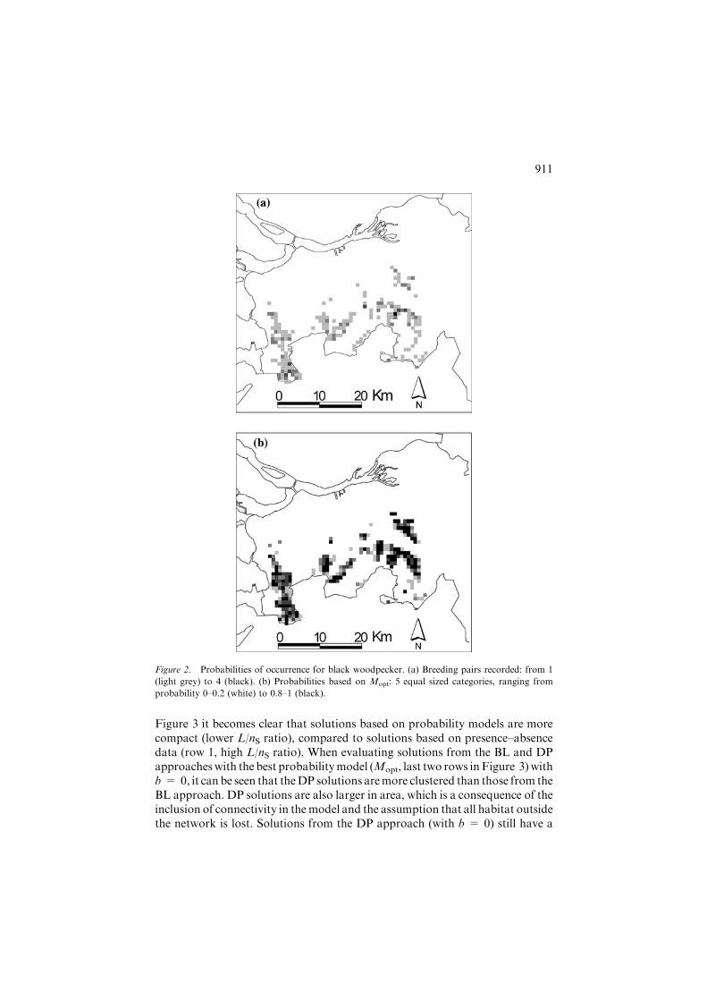
Figure 3 it becomes clear that solutions based on probability models are morecompact (lower L/nS ratio), compared to solutions based on presence–absencedata (row 1, high L/nS ratio). When evaluating solutions from the BL and DPapproacheswith the best probabilitymodel (Mopt, last two rows inFigure 3)withb = 0, it can be seen that theDP solutions aremore clustered than those from theBL approach. DP solutions are also larger in area, which is a consequence of theinclusion of connectivity in themodel and the assumption that all habitat outsidethe network is lost. Solutions from the DP approach (with b = 0) still have a

Figure 2. Probabilities of occurrence for black woodpecker. (a) Breeding pairs recorded: from 1

(light grey) to 4 (black). (b) Probabilities based on Mopt: 5 equal sized categories, ranging from

probability 0–0.2 (white) to 0.8–1 (black).

911

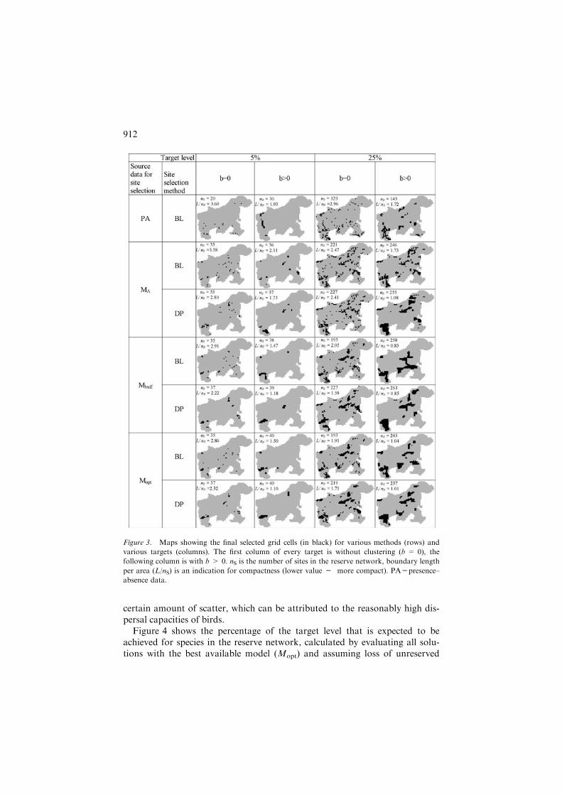
certain amount of scatter, which can be attributed to the reasonably high dis-persal capacities of birds.

Figure 4 shows the percentage of the target level that is expected to beachieved for species in the reserve network, calculated by evaluating all solu-tions with the best available model (Mopt) and assuming loss of unreserved

Figure 3. Maps showing the final selected grid cells (in black) for various methods (rows) and

various targets (columns). The first column of every target is without clustering (b = 0), the

following column is with b > 0. nS is the number of sites in the reserve network, boundary length

per area (L/nS) is an indication for compactness (lower value = more compact). PA=presence–

absence data.

912

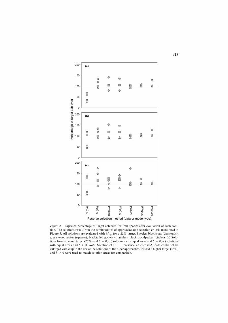
Figure 4. Expected percentage of target achieved for four species after evaluation of each solu-

tion. The solutions result from the combinations of approaches and selection criteria mentioned in

Figure 3. All solutions are evaluated with Mopt for a 25% target. Species: bluethroat (diamonds),

green woodpecker (squares), blacktailed godwit (triangles), black woodpecker (circles). (a) Solu-

tions from an equal target (25%) and b = 0; (b) solutions with equal areas and b = 0; (c) solutions

with equal areas and b > 0. Note: Solution of BL + presence–absence (PA) data could not be

enlarged with b up to the size of the solutions of the other approaches, instead a higher target (43%)

and b > 0 were used to match solution areas for comparison.

913

habitat. Results are shown for the four species for which the target level wasnot always achieved, for the other three species expected representation wasalways higher than the target level. In panel (A) all combinations of ap-proaches and selection criteria that were shown in Figure 3 with b = 0 andtarget = 25% are evaluated. Solutions produced with the BL approach do notreach the target levels for all species when evaluated with Mopt. When using aprobability model that does not take connectivity into account (i.e.MA) targetsare not achieved for blacktailed godwit and green woodpecker even when usingthe DP approach.

There are two possible causes for the species not to reach their target incertain solutions: the smaller size of the solution, or the lower level of con-nectivity in the solution. In order to estimate effects of solution size, wecompared solutions of similar size. Figure 4(b) shows results with comparablearea (nS = 224 ± 5 sites), achieved by increasing the target level for the BLapproach until network size is comparable to those networks obtained with theDP approach. Solutions were then evaluated against the lower target level, withwhich the DP solutions were obtained. When comparing panel (B) with (A), itfollows that with equal solution sizes the relative performances of solutionsfrom the BL approach increase, although for the bluethroat and the blacktailedgodwit the expected sum of occurrences is still below the target level. Addi-tionally, we compared solutions, which were comparable in size, produced witha penalty for boundary length (b > 0) to test whether additional clusteringwould improve the achieved target levels in the evaluation (Panel (C), target25%, b > 0, nS = 248 ± 11 sites). From panel (C) follows that when solu-tions are comparable in size and additional clustering is induced, for all speciesexcept the blacktailed godwit (and the bluethroat in case of presence–absencedata) the target can be achieved.

Discussion

The minimum set coverage approach (MC, represented by method BL withpresence–absence (PA) data and boundary penalty b = 0 in Figure 3, BL+ PA in Figure 4) does not use probability information and spatial consid-erations. It can therefore not acknowledge differences in site quality, and as aconsequence it performs poor in the evaluation with a spatially explicit prob-ability model. The performances of networks increase when probability modelsare used (BL + M in Figures 3 and 4), together with an increase in reservecompactness and size (Figure 3). As larger networks obviously protect a higherproportion of each species, similar sized solutions are compared in Figure 4(b).For few species the expected representation level is still not exceeding the targetrepresentation level, even though spatial models are used. Qualitative cluster-ing improves the expected number of occurrences of most species in the reservenetwork, although under-representation still occurs (Figure 4(c)). From thesetwo observations can be concluded that reserve networks based on models with

914

spatial measures rely to a certain extend on existing, but unreserved habitat(BL + Mbuff and Mopt), which persistence cannot be guaranteed for the fu-ture. These differences in performance between reserve networks lead to theconclusion that model choice is of importance to the size and spatial config-uration of the reserve network, which are again related to species persistence.These results support the common claim that reserve selection should not bebased on presence–absence data only, but incorporate spatial populationdynamics as well (Nicholls 1998; Hanski 1999; Cabeza and Moilanen 2001;Verboom et al. 2001).

Figure 4 also showed that the DP approach based onMA (habitat suitability)did not guarantee to sufficiently represent all species. Although theDP approachcan account for habitat loss outside the reserve, this is only effective whenprobabilities of occurrence depend on the set of selected sites (S) by includingmeasures of connectivity in the probabilities of occurrence. When probabilitiesof occurrence are based on habitat suitability only, habitat loss around thereserve cannot be evaluated by the probabilities of occurrence and is thus ig-nored. The use of connectivity measures in probability models is therefore a vitalelement in reserve design. We applied two simple measures of connectivity, thatboth were found to improve the model fit for all species but one. It is expectedthat connectivity measures will be significant for species with spatially structuredpopulations at scales that are in line with species’ dispersal ability.

Solutions obtained with Mbuff or Mopt do not seem to differ much in per-formance (Figure 4) and the addition of the IFM connectivity measure to themodel had only a small effect in AIC criteria and model evaluation. This is mostlikely due to scale issues. The dispersal capacities of the species are relativelylarge compared to the scale of the study area. Therefore it is possible thatsolutions produced by the DP approach with Mopt consist of several clusters ofsites within dispersal distance from each other. Solutions produced with Mbuff

on the other hand are expected to be more compact, since in Mbuff onlyneighbouring sites with suitable habitat contribute to the probabilities ofoccurrence in focal sites, whereas more distant sites do not. The effect of habitatloss is therefore stronger in solutions produced withMbuff than in solutions withMopt (compare the difference in compactness between DP solutions with Mbuff

andMopt (b = 0) in Figure 3, solutions withMbuff are more compact than thosewith Mopt. This is not the case for the BL approach, where there is no effect ofhabitat loss). Results may be different when dealing with different species orspatial scales. Cabeza (2003) has applied the DP approach to a dataset ofbutterflies (relatively limited dispersal capacities, given the size of the system),with probabilities of occurrence based on habitat suitability and buffer con-nectivity or IFM connectivity. In that study highly aggregated reserves werefound when loss of unprotected habitat was assumed, even without additionalclustering (i.e. b = 0). The choice for species and scale at which reserve design isapplied will therefore have a large influence on the spatial aggregation of thereserve network. Our results show that it is worth getting information onhabitat suitability and dispersal ability of as many species as possible. When

915

species-specific parameters are available it is possible to evaluate differentsolutions and scenarios for each species. If these parameters are not available, anon-species-specific buffer measure can be included, through which effects oflandscape change around the reserve network can be evaluated. When noconnectivity measures are included solutions with qualitative clustering (b > 0)perform better in terms of expected number of populations than non-spatialminimum set proportional coverage approaches (Figure 4(c)).

What follows from the evaluation of the solutions with Mopt and assumingcomplete habitat loss outside reserves is that probabilities inside the reservenetwork can be heavily affected by the occurrence of habitat outside the reservenetwork. The assumption of complete habitat loss might sound strong, but inhuman dominated landscapes (such as the Netherlands), it is quite likely thatunprotected natural areas will eventually turn into urban or agricultural land.Note also, that habitat transformation might negatively affect dispersal acrossunprotected habitat, which was not accounted for here. Another unaccountedeffect is that probabilities of occurrence near the boundary of the reserve mayactually decrease due to edge effects (Woodroffe and Ginsberg 1998; Debinskiand Holt 2000). Consequently, the effects of habitat loss might for some speciesbe even stronger than what was assumed here. More complex models of habitatchange could be combined with the DP approach to model the effects ofvarious scenarios of land use change (and/or habitat loss) on species’ proba-bilities of occurrence. Further, it is important to acknowledge and communi-cate uncertainties that accompany the use of observation data and modellingoccurrence to users of reserve selection methods (Elith et al. 2002; Regan et al.2002). Such uncertainties can include species observation errors (Wintle et al.2004), habitat classification errors, misclassification of true causal variables (bynot accounting for correlation between variables, or spatially autocorrelateddata) (Legendre et al. 2002), as well as insufficient model evaluation. Ourresults show that different reserve selection methods find optimal solutions thatdiffer consistently from each other with respect to the expected number ofpopulations they support. This suggests that careful attention should be givento the construction and evaluation of a proper species-specific probabilitymodel, and that the reserve selection algorithm should make reasonableassumptions about spatial population dynamics and effects of landscapedynamics.

Acknowledgements

Special thanks to H. Sierdsema, R. Foppen, R. Pouwels and J. Verboom foraccess to the data and additional information. Funding for this study wasreceived from the EU Socrates programme and Wageningen University(A.v.T.) and Academy of Finland research grants #71516 and #45125 to A.M.and M.C., respectively.

916

References

Araujo M.B. and Williams P.H. 2000. Selecting areas for species persistence using occurrence data.

Biol. Conserv. 96: 331–345.

Araujo M.B., Williams P.H. and Turner A. 2002. A sequential approach to minimise threats within

selected conservation areas. Biodiversity Conserv. 11: 1011–1024.

Austin M.P., Cunningham R.B. and Fleeming P.M. 1984. New approaches to direct gradient

analysis using environmental scalars and statistical curve-fitting procedures. Vegetatio 55: 11–27.

Briers R.A. 2002. Incorporating connectivity into reserve selection procedures. Biol. Conserv. 103:

77–83.

Cabeza M. 2003. Habitat loss and connectivity of reserve networks in probability approaches to

reserve design. Ecol. Lett. 6: 665–672.

Cabeza M. and Moilanen A. 2001. Design of reserve networks and the persistence of biodiversity.

Trends Ecol. Evol. 16: 242–248.

Cabeza M. and Moilanen A. 2003. Site selection algorithms and habitat loss. Conserv. Biol. 17:

1402–1413.

Cabeza M., Araujo M.B., Wilson R.J., Thomas C.D., Cowley M.J.R. and Moilanen A. 2004a.

Combining probabilities of occurrence with spatial reserve design. J. Appl. Ecol. 41: 252–262.

Cabeza M., Moilanen A. and Possingham H.P. 2004b. Metapopulation dynamics and reserve

network design. In: Hanski I. and Gaggiotti O. (eds), Metapopulation Ecology, Genetics, and

Evolution, Academic Press.

Csuti B., Polasky S., Williams P.H., Pressey R.L., Camm J.D., Kershaw M., Kiester A.R., Downs

B., Hamilton R., Huso M. and Sahr K. 1997. A comparison of reserve selection algorithms using

data on terrestrial vertebrates in Oregon. Biol. Conserv. 80: 83–97.

Debinski D.M. and Holt R.D. 2000. A survey and overview of habitat fragmentation experiments.

Conserv. Biol. 14: 342–355.

D’Eon R.G., Glenn S.M., Parfitt I. and Fortin M. 2002. Landscape connectivity as a function of

scale and organism vagility in a real forested landscape. Conserv. Ecol. 6: 10.

Elith J. 2000. Quantitative methods for modeling species habitat: comparative performance and an

application to Australian plants. In: Ferson S. and Burgman M. (eds), Quantitative Methods for

Conservation Biology. Springer, New York, pp. 39–58.

Elith J., Burgman M.A. and Regan H.M. 2002. Mapping epistemic uncertainties and vague con-

cepts in predictions of species distribution. Ecol. Model. 157: 313–329.

Ferrier S., Watson G., Pearce J. and Drielsma M. 2002. Extended statistical approaches to mod-

elling spatial pattern in biodiversity in northeast New South Wales. I. Species-level modelling.

Biodiversity Conserv. 11: 2275–2307.

Fielding A.H. and Bell J.F. 1997. A review of methods for the assessment of prediction errors in

conservation presence/absence models. Environ. Conserv. 24: 38–49.

Gaston K.J., Pressey R.L. and Margules C.R. 2002. Persistence and vulnerability: retaining bio-

diversity in the landscape and in protected areas. J. Biosci. 27: 361–384.

Grashof-Bokdam C. 1997. Forest species in an agricultural landscape in the Netherlands: effects of

habitat fragmentation. J. Vegetat. Sci. 8: 21–28.

Hanley J.A. and McNeil B.J. 1982. The meaning and use of the area under the receiver operating

characteristic (ROC) curve. Radiology 143: 29–36.

Hanski I. 1994. A practical model of metapopulation dynamics. J. Anim. Ecol. 63: 151–162.

Hanski I. 1999. Metapopulation Ecology. Oxford University Press, Oxford.

Heijnis C.E., Lombard A.T., Cowling R.M. and Desmet P.G. 1999. Picking up the pieces: a

biosphere reserve framework for a fragmented landscape – the coastal lowlands of the Western

Cape, South Africa. Biodiversity Conserv. 8: 471–496.

Howard P.C., Viskanic P., Davenport T.R.B., Kigenyi F.W., Baltzer M., Dickinson C.J., Lwanga

J.S., Matthews R.A. and Balmford A. 1998. Complementarity and the use of indicator groups

for reserve selection in Uganda. Nature 394: 472–475.

917

Kirkpatrick J.B. 1983. An iterative method for establishing priorities for the selection of nature

reserves: an example from Tasmania. Biol. Conserv. 25: 127–134.

Legendre P., Dale M.R.T., Fortin M., Gurevitch J., Hohn M. and Myers D. 2002. The conse-

quences of spatial structure for the design and analysis of ecological field surveys. Ecography 25:

601–615.

Manel S., Williams H.C. and Ormerod S.J. 2001. Evaluating presence–absence models in ecology:

the need to account for prevalence. J. Appl. Ecol. 38: 921–931.

Margules C.R., Cresswell I.D. and Nicholls A.O. 1994. A scientific basis for establishing networks

of protected areas. In: Forey P.L., Humphries C.J. and Vane-Wright R.I. (eds), Systematics and

Conservation Evaluation. Oxford University Press, Oxford, pp. 327–350.

Margules C.R., Nicholls A.O. and Pressey R.L. 1988. Selecting networks of reserves to maximise

biological diversity. Biol. Conserv. 43: 63–76.

Margules C.R., Pressey R.L. and Williams P.H. 2002. Representing biodiversity: data and pro-

cedures for identifying priority areas for conservation. J. Biosci. 27: 309–326.

Margules C.R. and Stein J.L. 1989. Patterns in the distributions of species and the selection of

nature reserves an example from eucalyptus forests in south-eastern New South Wales Australia.

Biol. Conserv. 50: 219–238.

Moilanen A. and Cabeza M. 2002. Single-species dynamic site selection. Ecol. Appl. 12: 913–926.

Moilanen A. and Nieminen M. 2002. Simple connectivity measures in spatial ecology. Ecology 83:

1131–1145.

Nalle D.J., Arthur J.L. and Sessions J. 2002. Designing compact and contiguous reserve networks

with a hybrid heuristic algorithm. Forest Sci. 48: 59–68.

Nicholls A.O. 1998. Integrating population abundance, dynamics and distribution into broad-scale

priority setting. In: Mace G., Balmford A. and Ginsberg J.R. (eds), Conservation in A Changing

World. Cambridge University Press, Cambridge.

Nicholls A.O. and Margules C.R. 1993. An upgraded reserve selection algorithm. Biol. Conserv.

64: 165–169.

Osborne P.E., Alonso J.C. and Bryant R.G. 2001. Modelling landscape-scale habitat use using GIS

and remote sensing: a case study with great bustards. J. Appl. Ecol. 38: 458–472.

Pearce J. and Ferrier S. 2000. Evaluating the predictive performance of habitat models developed

using logistic regression. Ecol. Model. 133: 225–245.

Possingham H.P., Ball I. and Andelman S. 2000. Mathematical methods for identifying repre-

sentative reserve network. In: Ferson S. and Burgman M. (eds), Quantitative Methods for

Conservation Biology. Springer, New York, pp. 291–306.

Pouwels R., Reijnen M.J.S.M., Kalkhoven J.T.R. and Dirksen J. 2002. Ecoprofielen voor so-

ortanalyses van ruimtelijke samenhang met LARCH. Alterra rapport 493, Alterra. Research

Instituut voor de Groene Ruimte, Wageningen.

Pressey R.L., Humphries C.J., Margules C.R., Vane-Wright R.I. and Williams P.H. 1993. Beyond

opportunism: key principles for systematic reserve selection. Trends Ecol. Evol. 8: 124–128.

R Development Core Team 2003. R: a language and environment for statistical computing.

R Foundation for Statistical Computing, Vienna, Austria.

Regan H.M., Colyvan M. and Burgman M.A. 2002. A taxonomy and treatment of uncertainty for

ecology and conservation biology. Ecol. Appl. 12: 618–628.

Reijnen R., Jochem R., De Jong M., De Heer M. and Sierdsema H. 2001. Larch Vogels Nationaal.

Een expertsysteem voor het beoordelen van de ruimtelijke samenhang en de duurzaamheid van

broedvogelpopulaties in Nederland. Alterra rapport 235, Alterra, Research Instituut voor de

Groene Ruimte, Wageningen.

Rodrigues A.S.L., Gregory R.D. and Gaston K.J. 2000. Robustness of reserve selection procedures

under temporal species turnover. Proc. Roy. Soc. Biol. Sci. Ser. B 267: 49–55.

Schumaker N.H. 1996. Using landscape indices to predict habitat connectivity. Ecology 77: 1210–

1225.

Swets J.A. 1988. Measuring the accuracy of diagnostic systems. Science 240: 1285–1293.

918

Ter Braak C.J.F. and Looman C.W.N. 1986. Weighted averaging, logistic regression and the

Gaussian response model. Vegetatio 65: 3–11.

Van Langevelde F. 2000. Scale of habitat connectivity and colonization in fragmented nuthatch

populations. Ecography 23: 614–622.

Van Langevelde F., Schotman A., Claassen F. and Sparenburg G. 2000. Competing land use in the

reserve site selection problem. Landscape Ecol. 15: 243–256.

Verboom J., Foppen R., Chardon P., Opdam P. and Luttikhuizen P. 2001. Introducing the key

patch approach for habitat networks with persistent populations: an example for marshland

birds. Biol. Conserv. 100: 89–101.

Virolainen K.M., Virola T., Suhonen J., Kuitunen M., Lammi A. and Siikamaki P. 1999. Selecting

networks of nature reserves: methods do affect the long-term outcome. Proc. Roy. Soc. Lond. B

266: 1141–1146.

Vogelonderzoek Nederland SOVON 2002. Atlas van de Nederlandse broedvogels 1998–2000,

Nederlandse fauna 5. Nationaal Natuurhistorisch Museum Naturalis, KNNV Uitgeverij &

European Invertebrate Survey, Nederland, Leiden.

Williams P.H. 1998. Key sites for conservation: area-selection methods for biodiversity. In: Mace

G., Balmford A. and Ginsberg J.R. (eds), Conservation in A Changing World. Cambridge

University Press, Cambridge.

Williams P.H. and Araujo M.B. 2000. Using probability of persistence to identify important areas

for biodiversity conservation. Proc. Roy. Soc. Biol. Sci. Ser. B 267: 1959–1966.

Williams P.H. and Araujo M.B. 2002. Apples, oranges, and probabilities: Integrating multiple

factors into biodiversity conservation with consistency. Environ. Model. Assess. 7: 139–151.

Wintle B.A., McCarthy M., Parris K.P. and Burgman M.A. 2004. Precision and bias of methods

for estimating point survey detection probabilities. Ecol. Appl. 14: 703–712.

With K., Gardner R.H. and Turner M.G. 1997. Landscape connectivity and population distri-

butions in heterogeneous environments. Oikos 78: 151–169.

Woodroffe R. and Ginsberg J.R. 1998. Edge effects and the extinction of populations inside

protected areas. Science 280: 2126–2128.

919