Journal of Computational Geometry jocg.org

COMPUTING MULTIDIMENSIONAL PERSISTENCE∗

Gunnar Carlsson,† Gurjeet Singh,‡ and Afra Zomorodian§

Abstract. The theory of multidimensional persistence captures the topology of a mul-tifiltration – a multiparameter family of increasing spaces. Multifiltrations arise naturallyin the topological analysis of scientific data. In this paper, we give a polynomial timealgorithm for computing multidimensional persistence. We recast this computation as aproblem within computational commutative algebra, and utilize algorithms from this areato solve it. While the resulting problem is Expspace-complete and the standard algorithmstake doubly-exponential time, we exploit the structure inherent within multifiltrations toyield practical algorithms. We implement all algorithms in the paper and provide statisticalexperiments to demonstrate their feasibility.

1 Introdu tion

In this paper, we give a polynomial time algorithm for computing the persistent homologyof a multifiltration. The computed solution is compact and complete, but not a topologicalinvariant. Theoretically, this is the best one may hope for because compact complete invari-ants do not exist for multidimensional persistence [2]. We discuss computing an incompleteinvariant, the rank invariant, and give an algorithm for reading off this invariant fromthe complete solution. We implement all algorithms in the paper and provide statisticalexperiments to demonstrate their feasibility.

1.1 Motivation

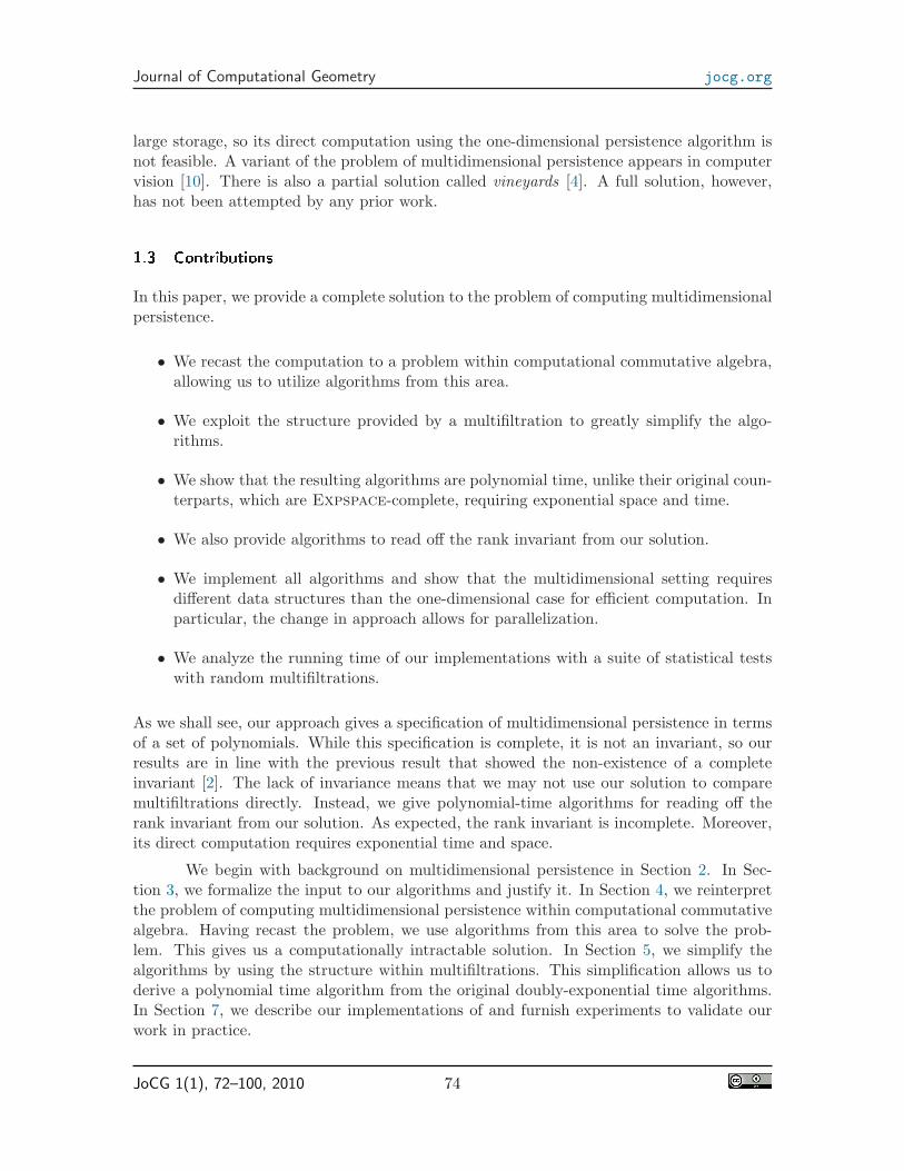
Intuitively, a multifiltration models a growing space that is parameterized along multipledimensions. For example, the complex with coordinate (3, 2) in Figure 1 is filtered alongthe horizontal and vertical dimensions, giving rise to a bifiltration. Multifiltrations arisenaturally in topological analysis of scientific data. Often, such data is in the form of afinite set of noisy samples from some underlying topological space. Our goal is to robustlyrecover the lost connectivity of the underlying space. If the sampling is dense enough,we may approximate the space as a union of balls by placing ǫ-balls around each point.As we increase ǫ, we obtain a growing family of spaces, a 1-dimensional multifiltration,

∗The authors were partially supported by the following grants: G. C. by NSF DMS-0354543; A. Z. byDARPA HR 0011-06-1-0038, ONR N 00014-08-1-0908, and NSF CCF-0845716; all by DARPA HR 0011-05-1-0007. A portion of the work was done while the second author was at Stanford University.

†Stanford University, gunnar@math.stanford.edu‡Ayasdi, Inc., gurjeet@ayasdi.com§Dartmouth College, afra@cs.dartmouth.edu

JoCG 1(1), 72–100, 2010 72

Journal of Computational Geometry jocg.org

(0,2)

(0,1)

(0,0)

(1,2)

(1,1)

(1,0)

(3,2)

(3,1)

(3,0)

(2,2)

(2,1)

(2,0)

a

b

cd

e

f

a

f b

ce

ce

bf af ab

bc

cdded

ef

cde

abf

Figure 1: A bifiltration. The complex with labeled vertices is at coordinate (3, 2). Simplicesare highlighted and named at the critical coordinates that they appear.

also called a filtration. This approximation is the central idea behind many methods forcomputing the topology of a point set [22]. Often, however, the input point set is filteredvia multiple functions. For instance, in analyzing the structure of natural images, we filterthe data according to density [1]. We now have multiple dimensions along which our spaceis filtered. That is, we have a multifiltration.

We characterize a multifiltration through invariants. An invariant is a function thatassigns identical objects to isomorphic structures. The trivial invariant assigns the sameobject to all structures, and is useless. The complete invariant assigns different objects tonon-isomorphic structures, and is powerful. We want to obtain a discrete invariant: aninvariant that yields a finite description and is not dependent on the underlying field ofcomputation [2]. Therefore, in the ideal setting, we would like a complete discrete invariantfor the structure of a multifiltration.

1.2 Prior Work

For one-dimensional filtrations, the theory of persistent homology provides a complete dis-crete invariant called a barcode, a multiset of intervals [23]. Each interval in the barcodecorresponds to the lifetime of a single topological feature within the filtration. Since intrin-sic features have long lives, while noise is short-lived, a quick examination of the intervalsgives a robust estimation of the topology. The existence of a complete discrete invariant, aswell as efficient algorithms and fast implementations have led to successful applications ofpersistent homology to a variety of problems, such as shape description [5], denoising vol-umetric density data [12], detecting holes in sensor networks [7], analyzing neural activityin the visual cortex [18], and analyzing the structure of natural images [1], to name a few.

For multifiltrations of dimension higher than one, the situation is much more compli-cated. The theory of multidimensional persistence shows that no complete discrete invariantexists. Instead, the authors propose an incomplete invariant, the rank invariant, which cap-tures some persistent information. Unfortunately, this invariant is not compact, requiring

JoCG 1(1), 72–100, 2010 73

Journal of Computational Geometry jocg.org

large storage, so its direct computation using the one-dimensional persistence algorithm isnot feasible. A variant of the problem of multidimensional persistence appears in computervision [10]. There is also a partial solution called vineyards [4]. A full solution, however,has not been attempted by any prior work.

1.3 Contributions

In this paper, we provide a complete solution to the problem of computing multidimensionalpersistence.

• We recast the computation to a problem within computational commutative algebra,allowing us to utilize algorithms from this area.

• We exploit the structure provided by a multifiltration to greatly simplify the algo-rithms.

• We show that the resulting algorithms are polynomial time, unlike their original coun-terparts, which are Expspace-complete, requiring exponential space and time.

• We also provide algorithms to read off the rank invariant from our solution.

• We implement all algorithms and show that the multidimensional setting requiresdifferent data structures than the one-dimensional case for efficient computation. Inparticular, the change in approach allows for parallelization.

• We analyze the running time of our implementations with a suite of statistical testswith random multifiltrations.

As we shall see, our approach gives a specification of multidimensional persistence in termsof a set of polynomials. While this specification is complete, it is not an invariant, so ourresults are in line with the previous result that showed the non-existence of a completeinvariant [2]. The lack of invariance means that we may not use our solution to comparemultifiltrations directly. Instead, we give polynomial-time algorithms for reading off therank invariant from our solution. As expected, the rank invariant is incomplete. Moreover,its direct computation requires exponential time and space.

We begin with background on multidimensional persistence in Section 2. In Sec-tion 3, we formalize the input to our algorithms and justify it. In Section 4, we reinterpretthe problem of computing multidimensional persistence within computational commutativealgebra. Having recast the problem, we use algorithms from this area to solve the prob-lem. This gives us a computationally intractable solution. In Section 5, we simplify thealgorithms by using the structure within multifiltrations. This simplification allows us toderive a polynomial time algorithm from the original doubly-exponential time algorithms.In Section 7, we describe our implementations of and furnish experiments to validate ourwork in practice.

JoCG 1(1), 72–100, 2010 74

Journal of Computational Geometry jocg.org

2 Ba kground

In this section, we review the theory of multidimensional persistence. We begin by for-malizing multifiltrations. We then review a sequence of theories of homology: simplicial,persistent, and multidimensional. We end with a description of the rank invariant.

2.1 Multi�ltrations

Let N ⊆ Z be the set of non-negative integers and R be the set of real numbers. For vectorsin N

n or Rn, we say u ≤ v if ui ≤ vi for all 1 ≤ i ≤ n, and define the ≥ relation similarly. The

relations ≤,≥ form partial orders on Nn and R

n. A topological space X is multifiltered ifwe are given a family of subspaces {Xu}u, where u ∈ N

n, so that Xu ⊆ Xv whenever u ≤ v.We call the family of subspaces {Xu}u a multifiltration. A one-dimensional multifiltrationis called a filtration.

If X is a cell complex, all subsets Xu must also be cell complexes, as shown for abifiltered simplicial complex in Figure 1. A critical coordinate u for cell σ ∈ X is a minimalcoordinate, with respect to the partial order ≤, such that σ ∈ Xu. In a multifiltration, anypath with monotonically increasing coordinates is a filtration, such as any row or columnin the figure. Multifiltrations constitute the input to our algorithms. We motivate their useas a model for scientific data as well as formalize them in the next section.

2.2 Homology

Given a topological space, homology is a topological invariant that is often used in practiceas it is easily computable. Here, we describe simplicial homology briefly, referring the readerto Hatcher [13] as a resource. We assume our input is a simplicial complex K, such as thecomplexes in Figure 1. We note, however, that our results carry over to arbitrary cellcomplexes, such as simplicial sets [9], ∆-complexes [13], and cubical complexes [14].

The ith chain group Ci(K) of K is the free Abelian group on K’s set of oriented i-simplices. An element c ∈ Ci(K) is an i-chain, c =

∑

j nj [σj ], σj ∈ K with coefficients nj ∈Z. Given such a chain c, the boundary operator ∂i : Ci(K)→ Ci−1(K) is a homomorphismdefined linearly by its action on any simplex σ = [v0, v1, . . . , vi] ∈ c,

∂iσ =∑

j

(−1)j [v0, . . . , vj , . . . , vi],

where vj indicates that vj is deleted from the vertex sequence. The boundary operatorconnects the chain groups into a chain complex C∗:

· · · → Ci+1(K)∂i+1

−−−→ Ci(K)∂i−→ Ci−1(K)→ · · · . (1)

Using the boundary operator, we may define subgroups of Ci: the cycle group ker ∂i andthe the boundary group im ∂i+1. Since ∂i ◦ ∂i+1 ≡ 0, then im ∂i+1 ⊆ ker ∂i ⊆ Ci(K). Theith homology group is

Hi(K) = ker ∂i/ im ∂i+1, (2)

JoCG 1(1), 72–100, 2010 75

Journal of Computational Geometry jocg.org

and the ith Betti number is βi(K) = rankHi(K). Over field coefficients k, Hi is a k-vectorspace of dimension βi.

2.3 Persistent Homology

Given a multifiltration {Xu}u, the homology of each subspace Xu over a field k is a vectorspace. For instance, the bifiltered complex in Figure 1 has zeroth homology vector spacesisomorphic to the commutative diagram

k2 k2 k k

k2 k4 k3 k3

k4 k3 k2 k2

// // //

//

OO

//

OO

//

OO OO

//

OO

//

OO

//

OO OO

where the dimension of the vector space counts the number of components of the complex,and the maps between the homology vector spaces are induced by the inclusion maps relatingthe subspaces. Persistent homology captures information contained in the induced maps.There are two equivalent definitions that we use in this paper. The first definition wasoriginally for filtrations only [8], but was later extended to multifiltrations [2]. The key ideais to relate the homologies of a pair of complexes. For each pair u, v ∈ N

n with u ≤ v,Xu ⊆ Xv by definition, so Xu → Xv. This inclusion, in turn, induces a linear map ιi(u, v)at the ith homology level Hi(Xu)→ Hi(Xv) that maps a homology class within Xu to theone that contains it within Xv. The ith persistent homology is im ιi, the image of ιi for allpairs u ≤ v. This definition also enables the definition of an incomplete invariant. The ithrank invariant is

ρi(u, v) = rank ιi(u, v), (3)

for all pairs u ≤ v ∈ Nn, where ιi is defined above [2]. While this definition provides

intuition, it is inexpedient for theoretical development. For most of our paper, we use asecond definition of persistence that is grounded in algebraic topology, allowing us to utilizetools from commutative algebra for computation [23, 2].

2.4 Multidimensional Persisten e

The key insight for the second definition below is that the persistent homology of a multi-filtration is the homology of a single algebraic entity. This object encodes all the complexesvia polynomials that track cells through the multifiltration. To define our algebraic struc-ture, we need to first review graded modules over polynomials. A monomial in x1, . . . , xn

is a product of the formxv1

1 · xv2

2 · · ·xvnn

with vi ∈ N. We denote it xv, where v = (v1, . . . , vn) ∈ Nn. A polynomial f in x1, . . . , xn

and coefficients in field k is a finite linear combination of monomials, f =∑

v cvxv, with

cv ∈ k. The set of all such polynomials is denoted k[x1, . . . , xn]. For instance, 5x1x22−7x3

3 ∈

JoCG 1(1), 72–100, 2010 76

Journal of Computational Geometry jocg.org

k[x1, x2, x3]. An n-graded ring is a ring R equipped with a decomposition of Abelian groupsR ∼= ⊕vRv, v ∈ N

n so that multiplication has the property Ru · Rv ⊆ Ru+v. Elements ina single group Ru are called homogeneous. The set of polynomials form the n-gradedpolynomial ring, denoted An. This ring is graded by An

v = kxv, v ∈ Nn. An n-graded

module over an n-graded ring R is an Abelian group M equipped with a decompositionM ∼= ⊕v Mv, v ∈ N

n together with a R-module structure so that Ru ·Mv ⊆ Mu+v. Ann-graded module is finitely generated if it admits a finite generating set. Also, recall thenotion of a free module on an n-graded set and a basis for such a module [2].

Given a multifiltration {Xu}u, the ith dimensional homology is the following n-graded module over An

⊕

u

Hi(Xu),

where the k-module structure is the direct sum structure and xv−u : Hi(Xu)→ Hi(Xv) is theinduced homomorphism ιi(u, v) we described in the previous section. This view of homologyyields two important results. In one dimension, the persistent homology of a filtration iseasily classified and parameterized by the barcode, and there is an efficient algorithm forits computation [23]. In higher dimensions, no similar classification exists [2]. Instead, wemay utilize an incomplete invariant. One such invariant, the rank invariant defined above,is provably equivalent to the barcode, and therefore complete, in one dimension, but it isincomplete in higher dimensions.

3 One-Criti al Multi�ltrations

We are interested in persistent homology as a tool for analyzing the topology of scientificdata. In this section, we begin by formalizing such data. We then show that topologicalanalysis of scientific data naturally generates multifiltrations. In particular, the processgenerates multifiltrations with the following property.

Definition 1 (one-critical). A multifiltered complex K where each cell σ has a uniquecritical coordinate uσ is one-critical.

In the rest of this paper, we assume that our input multifiltrations are one-critical.General multifiltrations, however, may not have this property. Therefore, we end thissection by describing a classic construction that eliminates multiple critical coordinates insuch input.

3.1 Model for S ienti� Data

We are often given scientific data in the form of a set of noisy samples from some underlyinggeometric space. At each sample point, we may also have measurements from the ambientspace. For example, a fundamental goal in graphics is to render objects under differentlighting from different camera positions. One approach is to construct a digitized modelusing data from a range scanner, which employs multiple cameras to sense 3D positions onan object’s surface, as well as estimated normals and texture information [19]. An alternate

JoCG 1(1), 72–100, 2010 77

Journal of Computational Geometry jocg.org

approach samples the four-dimensional light field of a surface directly and interpolates torender the object without explicit surface reconstruction [15]. Either approach gives us aset of noisy samples with measurements. Similarly, a node in a wireless sensor network hassensors on board that measure physical attributes of the local environment, such as pressureand temperature [21]. The GPS coordinates of the nodes constitute a set of samples at whichseveral functions are sampled.

Formally then, we assume we have a manifold X with n−1 Morse functions definedon it [16]. In practice, X is often embedded within a high-dimensional Euclidean space R

d,although this is not required. As such, we model the data using the following definition.

Definition 2 (multifiltered dataset). A multifiltered dataset is (S, {fj}j), where S is a finiteset of d-dimensional points with n − 1 real-valued functions fj : S → R defined on it, forn > 1.

3.2 Constru tion

We now assume our data is a multifiltered dataset (S, {fj}j). We begin by approximatingthe underlying space of S with a combinatorial representation, a complex, built on S. Thereare a variety of methods for building such complexes, all of which have a scale parameterǫ [22]. As we increase ǫ, a complex grows larger, and fixing a maximum scale ǫmax gives usa filtered complex K. Each cell σ ∈ K enters K at scale ǫ(σ). We formalize this type ofcomplex next.

Definition 3 (scale-filtered complex). A scale-filtered complex is the tuple (K, ǫ), whereK is a finite complex, ǫ : K → R, and the complexes Kµ = {σ | ǫ(σ) ≤ µ} form a one-dimensional filtration for K.

We assume we have a scale-filtered complex (K, ǫ) defined on our input point set S.To incorporate the functions fj into our data analysis, we first extend them to the cells inthe complex. For σ ∈ K and fj , let fj(σ) be the maximum value fj takes on σ’s vertices;that is, fj(σ) = maxv∈σ fj(v), where v ∈ S. This extension defines n − 1 functions on thecomplex, fj : K → R. We combine all filtration functions into a single multivariate functionF : K → R

n, where

F (σ) = (f1(σ), f2(σ), . . . , fn−1(σ), ǫ(σ)) .

We multifilter K via the excursion sets {Ku}u of F for u ∈ Rn:

Ku = {σ ∈ K | F (σ) ≤ u}.

Each simplex σ enters Ku at u = F (σ) and will remain in the complex for all u ≥ F (σ).Equivalently, F (σ) is the unique critical coordinate at which σ enters the filtered complex.That is, the multifiltrations built by the above process are always one-critical.

Example 1 (bifiltration criticals). The bifiltration in Figure 1 is one-critical, since eachsimplex enters at a single critical coordinate. For instance, F (a) = (1, 1), F (cde) = (3, 1),and F (af) = (1, 2).

JoCG 1(1), 72–100, 2010 78

Journal of Computational Geometry jocg.org

Since K is finite, we have a finite set of critical coordinates that we may projecton each dimension j to get a finite set of critical values Cj . We restrict ourselves tothe Cartesian product C1 × . . . × Cn of the critical values, parameterizing the resultingdiscrete grid using N in each dimension. This parameterization yields a a d-dimensionalmultifiltration {Kv}v with v ∈ N

n.

We end by noting that one-critical multifiltrations may be represented compactlyby the set of tuples

{(σ, F (σ)) | σ ∈ K} .

This representation is the main input to our algorithms in Section 4.3.

3.3 Mapping Teles ope

In general, multifiltrations are not one-critical since a cell may enter at multiple incompa-rable critical coordinates, viewing ≤ as a partial order on N

n. For example, in Figure 1, thevertex d that enters at (1, 0) may also enter at (0, 1) as the two coordinates are incompa-rable. For such multifiltrations, we may utilize the mapping telescope, a standard algebraicconstruction, to ensure that each cell has a unique critical coordinate [13]. Intuitively, thisconstruction introduces additional shadow cells into the multifiltration without changingits topology. We will not detail this construction here as none of the multifiltrations weencounter in practice require the conversion. We should note, however, that the mappingtelescope increases the size of the multifiltration, depending on the number of cells withmultiple critical points. In the worst case, the growth is exponential.

4 Using Computational Commutative Algebra

Having described our input, we next recast the problem of computing multidimensionalpersistence as a problem within computational commutative algebra. We then describestandard algorithms from this area that solve our problem. While this process gives us asolution, this solution is not practical as the algorithms are computationally intractable. Inthe next section, we refine them to derive polynomial-time algorithms.

4.1 Multigraded Homology

We begin by extending homology to multifiltered cell complexes. We then convert thecomputation of the latter to standard questions in computational commutative algebra.

Definition 4 (chain module). Given a multifiltered cell complex {Ku}u, the ith chainmodule is the n-graded module over An

Ci =⊕

u

Ci(Ku),

where the k-module structure is the direct sum structure and xv−u : Ci(Ku) → Ci(Kv) isthe inclusion Ku → Kv.

JoCG 1(1), 72–100, 2010 79

Journal of Computational Geometry jocg.org

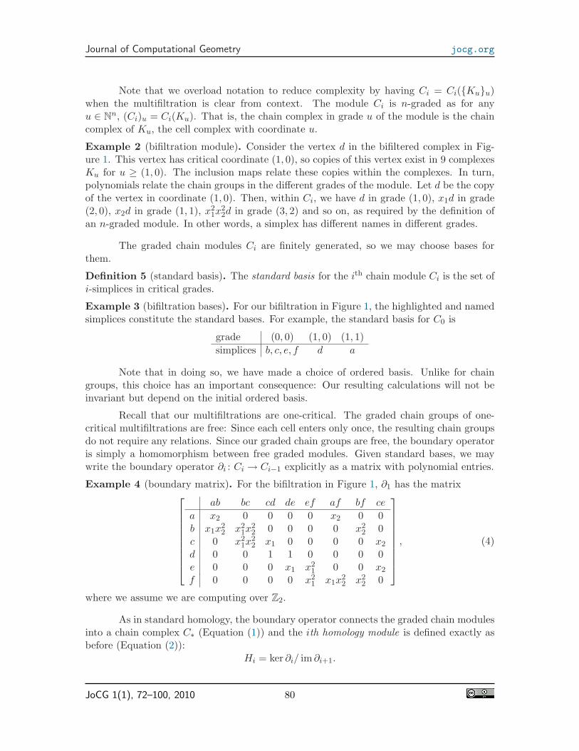
Note that we overload notation to reduce complexity by having Ci = Ci({Ku}u)when the multifiltration is clear from context. The module Ci is n-graded as for anyu ∈ N

n, (Ci)u = Ci(Ku). That is, the chain complex in grade u of the module is the chaincomplex of Ku, the cell complex with coordinate u.

Example 2 (bifiltration module). Consider the vertex d in the bifiltered complex in Fig-ure 1. This vertex has critical coordinate (1, 0), so copies of this vertex exist in 9 complexesKu for u ≥ (1, 0). The inclusion maps relate these copies within the complexes. In turn,polynomials relate the chain groups in the different grades of the module. Let d be the copyof the vertex in coordinate (1, 0). Then, within Ci, we have d in grade (1, 0), x1d in grade(2, 0), x2d in grade (1, 1), x2

1x22d in grade (3, 2) and so on, as required by the definition of

an n-graded module. In other words, a simplex has different names in different grades.

The graded chain modules Ci are finitely generated, so we may choose bases forthem.

Definition 5 (standard basis). The standard basis for the ith chain module Ci is the set ofi-simplices in critical grades.

Example 3 (bifiltration bases). For our bifiltration in Figure 1, the highlighted and namedsimplices constitute the standard bases. For example, the standard basis for C0 is

grade (0, 0) (1, 0) (1, 1)

simplices b, c, e, f d a

Note that in doing so, we have made a choice of ordered basis. Unlike for chaingroups, this choice has an important consequence: Our resulting calculations will not beinvariant but depend on the initial ordered basis.

Recall that our multifiltrations are one-critical. The graded chain groups of one-critical multifiltrations are free: Since each cell enters only once, the resulting chain groupsdo not require any relations. Since our graded chain groups are free, the boundary operatoris simply a homomorphism between free graded modules. Given standard bases, we maywrite the boundary operator ∂i : Ci → Ci−1 explicitly as a matrix with polynomial entries.

Example 4 (boundary matrix). For the bifiltration in Figure 1, ∂1 has the matrix

ab bc cd de ef af bf ce

a x2 0 0 0 0 x2 0 0b x1x

22 x2

1x22 0 0 0 0 x2

2 0c 0 x2

1x22 x1 0 0 0 0 x2

d 0 0 1 1 0 0 0 0e 0 0 0 x1 x2

1 0 0 x2

f 0 0 0 0 x21 x1x

22 x2

2 0

, (4)

where we assume we are computing over Z2.

As in standard homology, the boundary operator connects the graded chain modulesinto a chain complex C∗ (Equation (1)) and the ith homology module is defined exactly asbefore (Equation (2)):

Hi = ker ∂i/ im ∂i+1.

JoCG 1(1), 72–100, 2010 80

Journal of Computational Geometry jocg.org

4.2 Re asting the Problem

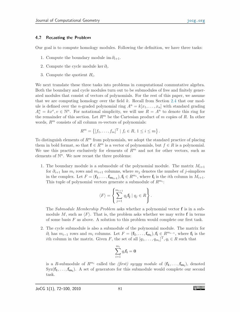
Our goal is to compute homology modules. Following the definition, we have three tasks:

1. Compute the boundary module im ∂i+1.

2. Compute the cycle module ker ∂i.

3. Compute the quotient Hi.

We next translate these three tasks into problems in computational commutative algebra.Both the boundary and cycle modules turn out to be submodules of free and finitely gener-ated modules that consist of vectors of polynomials. For the rest of this paper, we assumethat we are computing homology over the field k. Recall from Section 2.4 that our mod-ule is defined over the n-graded polynomial ring An = k[x1, . . . , xn] with standard gradingAn

v = kxv, v ∈ Nn. For notational simplicity, we will use R = An to denote this ring for

the remainder of this section. Let Rm be the Cartesian product of m copies of R. In otherwords, Rm consists of all column m-vectors of polynomials:

Rm ={

[f1, . . . , fm]T | fi ∈ R, 1 ≤ i ≤ m}

.

To distinguish elements of Rm from polynomials, we adopt the standard practice of placingthem in bold format, so that f ∈ Rm is a vector of polynomials, but f ∈ R is a polynomial.We use this practice exclusively for elements of Rm and not for other vectors, such aselements of N

n. We now recast the three problems:

1. The boundary module is a submodule of the polynomial module. The matrix Mi+1

for ∂i+1 has mi rows and mi+1 columns, where mj denotes the number of j-simplicesin the complex. Let F = (f1, . . . , fmi+1

), fi ∈ Rmi , where fi is the ith column in Mi+1.This tuple of polynomial vectors generate a submodule of Rmi :

〈F 〉 =

mi+1∑

j=1

qjfj | qj ∈ R

.

The Submodule Membership Problem asks whether a polynomial vector f is in a sub-module M , such as 〈F 〉. That is, the problem asks whether we may write f in termsof some basis F as above. A solution to this problem would complete our first task.

2. The cycle submodule is also a submodule of the polynomial module. The matrix for∂i has mi−1 rows and mi columns. Let F = (f1, . . . , fmi

), fi ∈ Rmi−1 , where fi is theith column in the matrix. Given F , the set of all [q1, . . . , qmi

]T, qi ∈ R such that

mi∑

i=1

qifi = 0

is a R-submodule of Rmi called the (first) syzygy module of (f1, . . . , fmi), denoted

Syz(f1, . . . , fmi). A set of generators for this submodule would complete our second

task.

JoCG 1(1), 72–100, 2010 81

Journal of Computational Geometry jocg.org

3. Our final task is simple, once we have completed the first two tasks. All we needto do is test whether the generators of the syzygy submodule, our cycles, are in theboundary submodule. As we shall see, the tools which allow us to complete the firsttwo tasks also resolve this question.

4.3 Algorithms

In this section, we begin by reviewing concepts from commutative algebra that involve thepolynomial module Rm We then look at algorithms for solving the submodule membershipproblem and computing generators for the syzygy submodule. In our treatment, we followChapter 5 of Cox, Little, and O’Shea [6].

The standard basis for Rm is {e1, . . . , em}, where ei is the standard basis vectorwith constant polynomials 0 in all positions except 1 in position i. We use the “top down”order on the standard basis vectors, so that ei > ej whenever i < j. A monomial m in Rm

is an element of the form xuei for some i and we say m contains ei.

For algorithms, we need to order monomials in both R and Rm. For u, v ∈ Nn, we

say u >lex v if the vector difference u− v ∈ Zn, the leftmost nonzero entry is positive. The

lexicographic order >lex is a total order on Nn. For example, (1, 3, 0) >lex (1, 2, 1) since

(1, 3, 0) − (1, 2, 1) = (0, 1,−1) and the leftmost nonzero entry is 1. Now, suppose xu andxv are monomials in R. We say xu >lex xv if u >lex v. This gives us a monomial order onR. We next extend >lex to a monomial order on Rm using the “position-over-term” (POT)rule: xuei > xvej if i < j, or if i = j and xu >lex xv. Every element f ∈ Rm may be written,in a unique way, as a k-linear combination of monomials mi,

f =∑

i

cimi, (5)

where ci ∈ k, ci 6= 0 and the monomials mi are ordered according to the monomial order.We define:

• Each cimi is a term of f .

• The leading coefficient of f is lc(f) = c1 ∈ k.

• The leading monomial of f is lm(f) = m1.

• The leading term of f is lt(f) = c1m1.

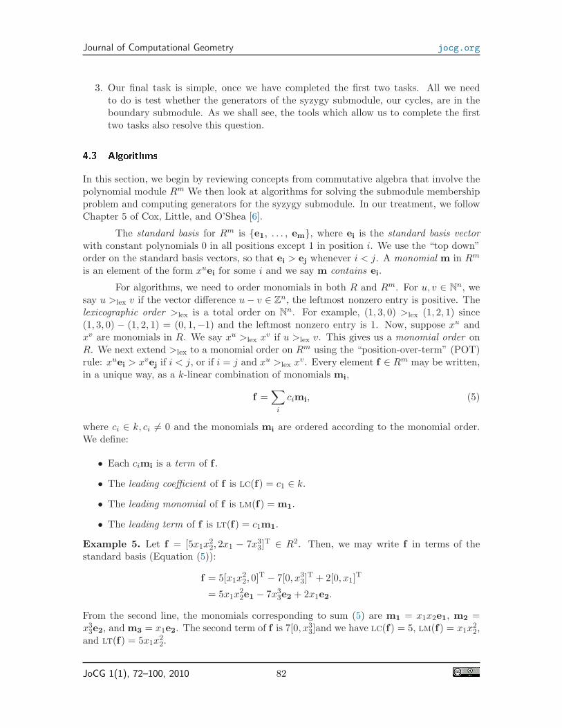
Example 5. Let f = [5x1x22, 2x1 − 7x3

3]T ∈ R2. Then, we may write f in terms of the

standard basis (Equation (5)):

f = 5[x1x22, 0]T − 7[0, x3

3]T + 2[0, x1]

T

= 5x1x22e1 − 7x3

3e2 + 2x1e2.

From the second line, the monomials corresponding to sum (5) are m1 = x1x2e1, m2 =x3

3e2, and m3 = x1e2. The second term of f is 7[0, x33]and we have lc(f) = 5, lm(f) = x1x

22,

and lt(f) = 5x1x22.

JoCG 1(1), 72–100, 2010 82

Journal of Computational Geometry jocg.org

Finally, we extend division and least common multiple to monomials in R and Rm.Given monomials xu, xv ∈ R, if v ≤ u, then xv divides xu with quotient xu/xv = xu−v.Now, let w ∈ N

n by wi = max(ui, vi) and define the monomial xw to be the least commonmultiple of xu and xv, denoted lcm(xu, xv) = xw. Next, given monomials m = xuei andn = xvej in Rm, we say n divides m iff i = j and xv divides xu, and define the quotient tobe m/n = xu/xv = xu−v. In addition, we define

lcm(xuei, xvej) =

{

lcm(xu, xv)ei, i = j,0, otherwise.

(6)

Clearly, the lcm of two monomials is a monomial in R and Rm, respectively.

Example 6. Let f = [x1, x1x2]T and g = [x2, 0]T be elements of R2. Then, the lcm of

their leading monomials is:

lcm(lm(f), lm(g)) = lcm(x1e1, x2e1)

= x1x2e1.

Recall the Submodule Membership Problem: Given a polynomial vector f and aset of t polynomials F , is f ∈ 〈F 〉? We may divide f by F using the division algorithmDivide in Figure 2. After division, we have f = (

∑ti=1 qifi) + r, so if the remainder r = 0,

then f ∈ 〈F 〉. This condition, however, is not necessary for modules over multivariatepolynomials as we may get a non-zero remainder even when f ∈ 〈F 〉.

Let M be an submodule and lt(M) be the set of leading terms of elements of M .A Grobner basis is a basis G ⊆ M such that 〈lt(G)〉 = 〈lt(M)〉. If f ∈ 〈F 〉, we alwaysget r = 0 after division of f by a Grobner basis for 〈F 〉, so we have solved the membershipproblem. The Buchberger algorithm in Figure 3 computes a Grobner basis G startingfrom any basis F . The algorithm utilizes S-polynomials on line 4 to eliminate the leading

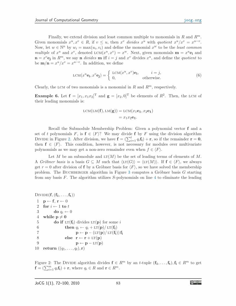
Divide(f , (f1, . . . , ft))

1 p← f , r← 02 for i← 1 to t3 do qi ← 04 while p 6= 0

5 do if lt(fi) divides lt(p) for some i6 then qi ← qi + lt(p)/ lt(fi)7 p← p− (lt(p)/ lt(fi)) fi8 else r← r + lt(p)9 p← p− lt(p)

10 return ((q1, . . . , qt), r)

Figure 2: The Divide algorithm divides f ∈ Rm by an t-tuple (f1, . . . , ft), fi ∈ Rm to getf = (

∑mi=1 qifi) + r, where qi ∈ R and r ∈ Rm.

JoCG 1(1), 72–100, 2010 83

Journal of Computational Geometry jocg.org

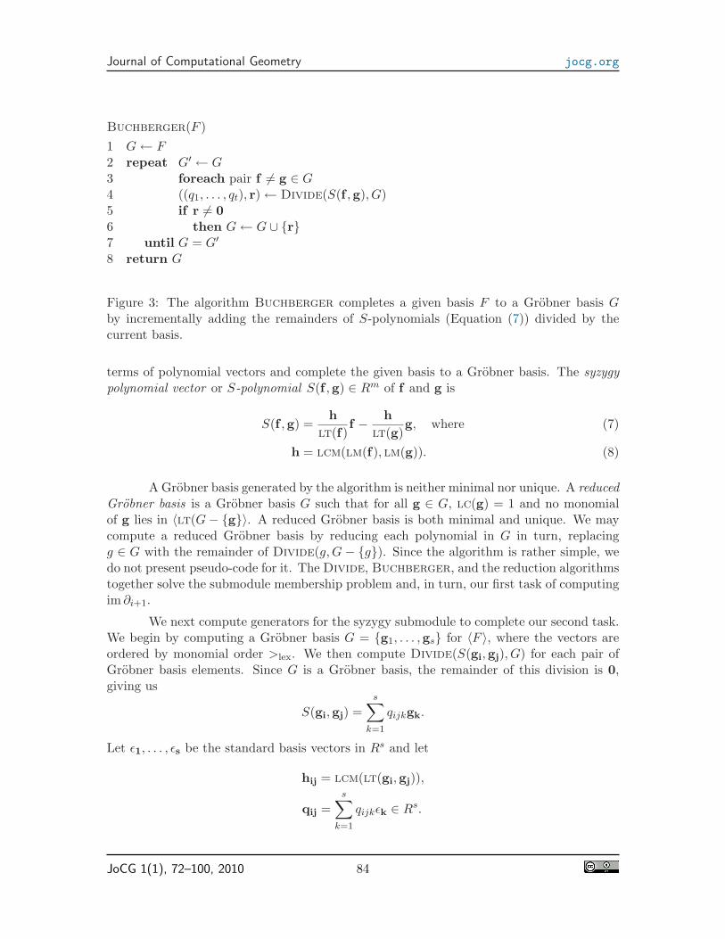
Buchberger(F )

1 G← F2 repeat G′ ← G3 foreach pair f 6= g ∈ G4 ((q1, . . . , qt), r)← Divide(S(f ,g), G)5 if r 6= 0

6 then G← G ∪ {r}7 until G = G′

8 return G

Figure 3: The algorithm Buchberger completes a given basis F to a Grobner basis Gby incrementally adding the remainders of S-polynomials (Equation (7)) divided by thecurrent basis.

terms of polynomial vectors and complete the given basis to a Grobner basis. The syzygypolynomial vector or S-polynomial S(f ,g) ∈ Rm of f and g is

S(f ,g) =h

lt(f)f −

h

lt(g)g, where (7)

h = lcm(lm(f), lm(g)). (8)

A Grobner basis generated by the algorithm is neither minimal nor unique. A reducedGrobner basis is a Grobner basis G such that for all g ∈ G, lc(g) = 1 and no monomialof g lies in 〈lt(G− {g}〉. A reduced Grobner basis is both minimal and unique. We maycompute a reduced Grobner basis by reducing each polynomial in G in turn, replacingg ∈ G with the remainder of Divide(g, G− {g}). Since the algorithm is rather simple, wedo not present pseudo-code for it. The Divide, Buchberger, and the reduction algorithmstogether solve the submodule membership problem and, in turn, our first task of computingim ∂i+1.

We next compute generators for the syzygy submodule to complete our second task.We begin by computing a Grobner basis G = {g1, . . . ,gs} for 〈F 〉, where the vectors areordered by monomial order >lex. We then compute Divide(S(gi,gj), G) for each pair ofGrobner basis elements. Since G is a Grobner basis, the remainder of this division is 0,giving us

S(gi,gj) =s

∑

k=1

qijkgk.

Let ǫ1, . . . , ǫs be the standard basis vectors in Rs and let

hij = lcm(lt(gi,gj)),

qij =s

∑

k=1

qijkǫk ∈ Rs.

JoCG 1(1), 72–100, 2010 84

Journal of Computational Geometry jocg.org

For pairs (i, j) such that hij 6= 0, we define sij ∈ Rs by

sij =hij

lt(gi)ǫi −

hij

lt(gj)ǫj − qij ∈ Rs,

with sij = 0, otherwise. Schreyer’s Theorem states that the set {sij}ij form a Grobner basisfor Syz(g1, . . . ,gs) [6, Chapter 5, Theorem 3.3]. Clearly, we may compute this basis usingDivide. We use this basis to find generators for Syz(f1, . . . , ft).

Let MF and MG be the m × t and m × s matrices in which the fi’s and gi’s arecolumns, respectively. As both bases generate the same module, there is a t × s matrixA and an s × t matrix B such that MG = MF A and MF = MGB. To compute A, weinitialize A to be the identity matrix and add a column to A for each division on line 4 ofBuchberger that records the pair involved in the S-polynomial. The matrix B may becomputed by using the division algorithm. To see how, notice that each column of MF isdivisible by MG since MG is a Grobner basis for MF . Now there is a column in B for eachcolumn fi ∈ MF , which is obtained by division of fi by MG. Let s1, . . . , st be the columnsof the t× t matrix It −AB. Then,

Syz(f1, . . . , ft) = 〈Asij, s1, . . . , st〉,

giving us the syzygy generators [6, Chapter 5, Proposition 3.8]. We refer to the algorithmsketched above as Schreyer’s algorithm. This algorithm completes the second task.

The third task is to compute the quotient Hi given im ∂i+1 = 〈G〉 and ker ∂i =Syz(f1, . . . , ft). We simply need to find whether the columns of ker ∂i can be represented asa combination of the basis for im ∂i+1. The modules Hi may be computed using the divisionalgorithm. We divide every column in ker ∂i by im ∂i+1 using the Divide algorithm. If theremainder is non-zero, we add the remainder both to im ∂i+1 and Hi so as to count onlyunique cycles.

A Grobner basis of a module depends on the choice of the ordered basis, so ourresulting specification of homology is not unique up to the module, and therefore, notan invariant. This means, for instance, that we cannot compare two Grobner bases todetermine if they represent the same module. That is, while our solution is complete, it isnot an invariant. For this reason, we give polynomial time algorithms to read off a discreteinvariant in Section 6 from our results. This invariant is, however, incomplete as predictedby prior work [2].

While the above algorithms solve the membership problem, they have not been usedin practice due to their complexity. The submodule membership problem is a generalizationof the Polynomial Ideal Membership Problem (PIMP) which is Expspace-complete, requir-ing exponential space and time [17, 20]. Indeed, the Buchberger algorithm, in its originalform, is doubly-exponential and is therefore not practical.

5 Multigraded Algorithms

In this section, we show that multifiltrations provide additional structure that may beexploited to simplify the algorithms from the previous section. These simplifications convert

JoCG 1(1), 72–100, 2010 85

Journal of Computational Geometry jocg.org

these intractable algorithms into polynomial time algorithms. Throughout this section, thefield k of coefficients is the field with two elements Z2, for simplicity. Our treatment,however, generalizes to any arbitrary field.

5.1 Exploiting Homogeneity

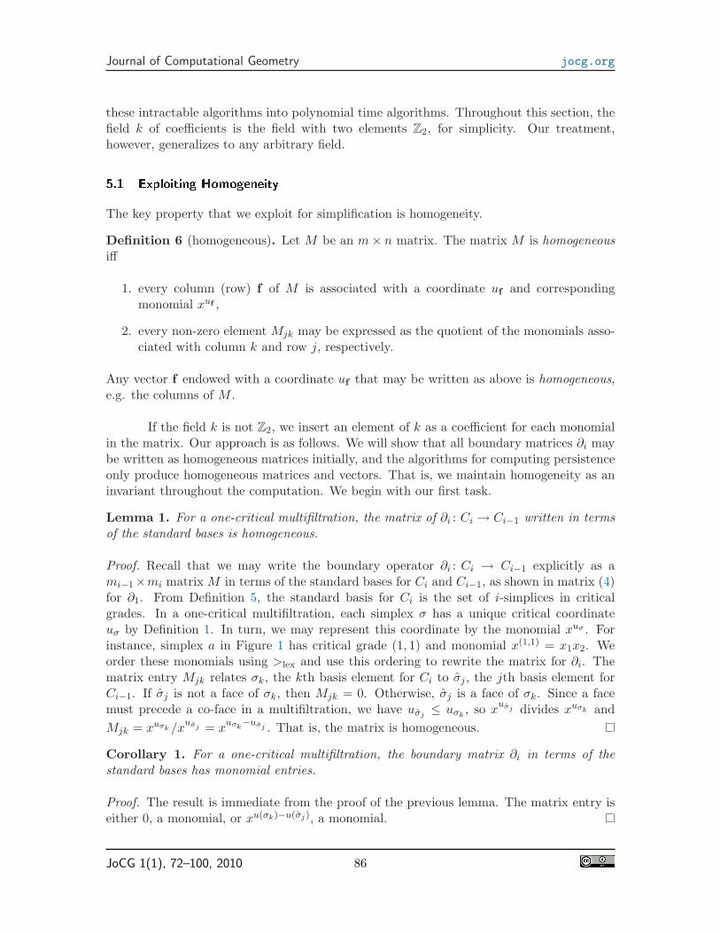
The key property that we exploit for simplification is homogeneity.

Definition 6 (homogeneous). Let M be an m× n matrix. The matrix M is homogeneousiff

1. every column (row) f of M is associated with a coordinate uf and correspondingmonomial xuf ,

2. every non-zero element Mjk may be expressed as the quotient of the monomials asso-ciated with column k and row j, respectively.

Any vector f endowed with a coordinate uf that may be written as above is homogeneous,e.g. the columns of M .

If the field k is not Z2, we insert an element of k as a coefficient for each monomialin the matrix. Our approach is as follows. We will show that all boundary matrices ∂i maybe written as homogeneous matrices initially, and the algorithms for computing persistenceonly produce homogeneous matrices and vectors. That is, we maintain homogeneity as aninvariant throughout the computation. We begin with our first task.

Lemma 1. For a one-critical multifiltration, the matrix of ∂i : Ci → Ci−1 written in termsof the standard bases is homogeneous.

Proof. Recall that we may write the boundary operator ∂i : Ci → Ci−1 explicitly as ami−1×mi matrix M in terms of the standard bases for Ci and Ci−1, as shown in matrix (4)for ∂1. From Definition 5, the standard basis for Ci is the set of i-simplices in criticalgrades. In a one-critical multifiltration, each simplex σ has a unique critical coordinateuσ by Definition 1. In turn, we may represent this coordinate by the monomial xuσ . Forinstance, simplex a in Figure 1 has critical grade (1, 1) and monomial x(1,1) = x1x2. Weorder these monomials using >lex and use this ordering to rewrite the matrix for ∂i. Thematrix entry Mjk relates σk, the kth basis element for Ci to σj , the jth basis element forCi−1. If σj is not a face of σk, then Mjk = 0. Otherwise, σj is a face of σk. Since a facemust precede a co-face in a multifiltration, we have uσj

≤ uσk, so x

uσj divides xuσk and

Mjk = xuσk /xuσj = x

uσk−uσj . That is, the matrix is homogeneous.

Corollary 1. For a one-critical multifiltration, the boundary matrix ∂i in terms of thestandard bases has monomial entries.

Proof. The result is immediate from the proof of the previous lemma. The matrix entry iseither 0, a monomial, or xu(σk)−u(σj), a monomial.

JoCG 1(1), 72–100, 2010 86

Journal of Computational Geometry jocg.org

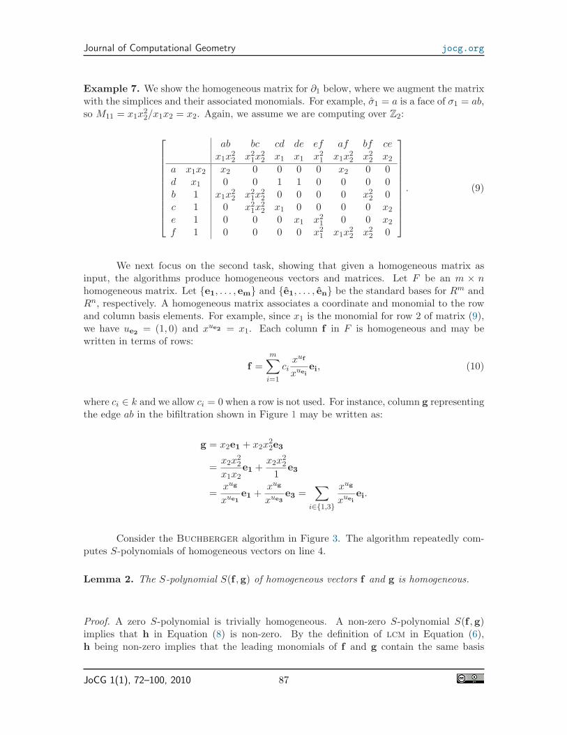
Example 7. We show the homogeneous matrix for ∂1 below, where we augment the matrixwith the simplices and their associated monomials. For example, σ1 = a is a face of σ1 = ab,so M11 = x1x

22/x1x2 = x2. Again, we assume we are computing over Z2:

ab bc cd de ef af bf cex1x

22 x2

1x22 x1 x1 x2

1 x1x22 x2

2 x2

a x1x2 x2 0 0 0 0 x2 0 0d x1 0 0 1 1 0 0 0 0b 1 x1x

22 x2

1x22 0 0 0 0 x2

2 0c 1 0 x2

1x22 x1 0 0 0 0 x2

e 1 0 0 0 x1 x21 0 0 x2

f 1 0 0 0 0 x21 x1x

22 x2

2 0

. (9)

We next focus on the second task, showing that given a homogeneous matrix asinput, the algorithms produce homogeneous vectors and matrices. Let F be an m × nhomogeneous matrix. Let {e1, . . . , em} and {e1, . . . , en} be the standard bases for Rm andRn, respectively. A homogeneous matrix associates a coordinate and monomial to the rowand column basis elements. For example, since x1 is the monomial for row 2 of matrix (9),we have ue2

= (1, 0) and xue2 = x1. Each column f in F is homogeneous and may bewritten in terms of rows:

f =m

∑

i=1

cixuf

xueiei, (10)

where ci ∈ k and we allow ci = 0 when a row is not used. For instance, column g representingthe edge ab in the bifiltration shown in Figure 1 may be written as:

g = x2e1 + x2x22e3

=x2x

22

x1x2e1 +

x2x22

1e3

=xug

xue1e1 +

xug

xue3e3 =

∑

i∈{1,3}

xug

xueiei.

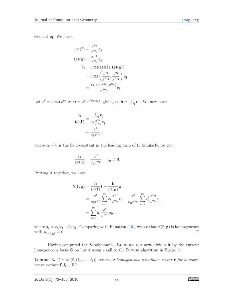
Consider the Buchberger algorithm in Figure 3. The algorithm repeatedly com-putes S-polynomials of homogeneous vectors on line 4.

Lemma 2. The S-polynomial S(f ,g) of homogeneous vectors f and g is homogeneous.

Proof. A zero S-polynomial is trivially homogeneous. A non-zero S-polynomial S(f ,g)implies that h in Equation (8) is non-zero. By the definition of lcm in Equation (6),h being non-zero implies that the leading monomials of f and g contain the same basis

JoCG 1(1), 72–100, 2010 87

Journal of Computational Geometry jocg.org

element ej. We have:

lm(f) =xuf

xuejej

lm(g) =xug

xuejej

h = lcm(lm(f), lm(g))

= lcm

(

xuf

xuej,

xug

xuej

)

ej

=lcm (xuf , xug)

xuejej.

Let xℓ = lcm(xuf , xug) = xlcm(uf ,ug), giving us h = xℓ

xuej

ej. We now have

h

lt(f)=

xℓ

xuej

ej

cfxuf

xuej

ej

=xℓ

cfxuf,

where cf 6= 0 is the field constant in the leading term of f . Similarly, we get

h

lt(g)=

xℓ

cgxug, cg 6= 0.

Putting it together, we have

S(f ,g) =h

lt(f)f −

h

lt(g)g

=xℓ

cfxuf

m∑

i=1

cixuf

xueiei −

xℓ

cgxug

m∑

i=1

c′ixug

xueiei

=m

∑

i=1

dixℓ

xueiei,

where di = ci/cf−c′i/cg. Comparing with Equation (10), we see that S(f ,g) is homogeneouswith uS(f ,g) = ℓ.

Having computed the S-polynomial, Buchberger next divides it by the currenthomogeneous basis G on line 4 using a call to the Divide algorithm in Figure 2.

Lemma 3. Divide(f , (f1, . . . , ft)) returns a homogeneous remainder vector r for homoge-neous vectors f , fi ∈ Rm.

JoCG 1(1), 72–100, 2010 88

Journal of Computational Geometry jocg.org

Proof. On line 1, r and p are initialized to be 0 and f , respectively, and are both triviallyhomogeneous. We will show that each iteration of the while loop starting on line 4 main-tains the homogeneity of these two vectors. On line 5, since both fi and p are homogeneous,we have

fi =m

∑

j=1

cijxufi

xuejej

p =m

∑

j=1

djxup

xuejej.

Since lt(fi) divides lt(p), the terms must share basis element ek and we have

lt(fi) = cikxufi

xuekek

lt(p) = dkxup

xuekek

lt(p)/ lt(fi) =dk

cik·xup

xufi.

On line 7, p is assigned to

p− (lt(p)/ lt(fi))fi =m

∑

j=1

djxup

xuejej −

(

dk

cik·xup

xufi

) m∑

j=1

cijxufi

xuejej

=m

∑

j=1

(

dj −dk · cij

cik

)

xup

xuejej

=m

∑

j=1

d′jxup

xuejej,

where d′j = dj − dk · cij/cik and d′k = 0, so the subtraction eliminates the kth term. Thefinal sum means that p is a new homogeneous polynomial with the same coordinate up

as before. Similarly, lt(p) is added to r on line 8 and subtracted from p on line 9, andneither action changes the homogeneity of either vector. Both remain homogeneous withcoordinate up.

The lemmas combine to give us the desired result.

Theorem 1 (homogeneous Grobner). Given a homogeneous basis, the Buchberger algo-rithm computes a homogeneous Grobner basis.

Proof. Initially, the algorithm sets G to be the input basis F , which is homogeneous. Online 4, it computes the S-polynomial of homogeneous vectors f ,g ∈ G. By Lemma 2, theS-polynomial is homogeneous. It then divides the S-polynomial by G. Since the inputis homogeneous, Divide produces a homogeneous remainder r by Lemma 3. Since onlyhomogeneous vectors are added to G on line 6, G remains homogeneous.

JoCG 1(1), 72–100, 2010 89

Journal of Computational Geometry jocg.org

We may extend this result easily to the reduced Grobner basis. Using similar argu-ments, we may show the following result, whose proof we omit here.

Theorem 2 (homogenous syzygy). For a homogeneous matrix, all matrices encountered inthe computation of the syzygy module are homogeneous.

5.2 Data Stru tures and Optimizations

We have shown that the structure inherent in a multifiltration allows us to compute usinghomogeneous vectors and matrices whose entries are monomials only. We next explorethe consequences of this restriction on both the data structures and complexity of thealgorithms.

By Definition (6), an m × n homogeneous matrix naturally associates monomialsto the standard bases for Rm and Rn. Moreover, every non-zero entry of the matrix isa quotient of these monomials as the matrix is homogeneous. Therefore, we do not needto store the matrix entries, but simply the field elements of the matrix along with themonomials for the bases. We may modify two standard data structures to represent thematrix.

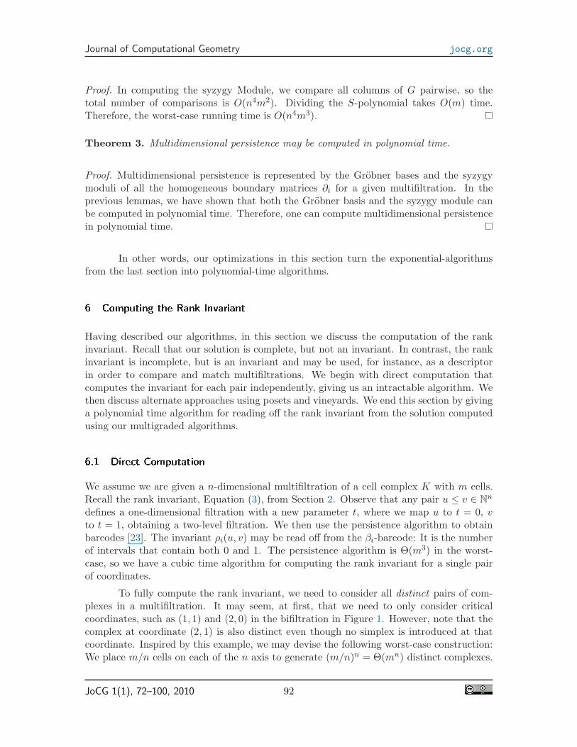
• linked list: Each column stores its monomial as well as a linked-list of its non-zeroentries in sorted order. The non-zero entries are represented by the row index and thefield element. The matrix is simply a list of these columns in sorted order. Figure 4displays matrix (9) in this data structure.

• matrix: Each column stores its monomial as well as the column of field coefficients.If we are computing over a finite field, we may pack bits for space efficiency.

The linked-list representation is appropriate for sparse matrices as it is space-efficient atthe price of linear access time. This is essentially the representation used for computing inthe one-dimensional setting [23]. In contrast, the matrix representation is appropriate fordense matrices as it provides constant access time at the cost of storing all zero entries. Themultidimensional setting provides us with denser matrices, as we shall see, so the matrixrepresentation becomes a viable structure.

In addition, the matrix representation is optimally suited to computing over the fieldZ2, the field often commonly employed in topological data analysis. The matrix entries each

Figure 4: The linked list representation of the boundary matrix ∂1 of Equation (4), for thebifiltration shown in Figure 1, in column sorted order. Note that the columns in Equation (4)are not ordered while they are sorted correctly here.

JoCG 1(1), 72–100, 2010 90

Journal of Computational Geometry jocg.org

take one bit and the column entries may be packed into machine words. Moreover, the onlyoperation required by the algorithms is symmetric difference which may be implemented asa binary XOR operation provided by the chip. This approach gives us bit-level parallelismfor free: On a 64-bit machine, we perform symmetric difference 64 times faster than on thelist. The combination of these techniques allow the matrix structure to perform better thanthe linked-list representation in practice.

We may also exploit homogeneity to speed up the computation of new vectors andtheir insertion into the basis. We demonstrate this briefly using the Buchberger algo-rithm. We order the columns of input matrix G using the POT rule for vectors as introducedin Section 4. Suppose we have f ,g ∈ G with f > g. If S(f ,g) 6= 0, lt(f) and lt(g) containthe same basis element, which the S-polynomial eliminates. So, we have S(f ,g) < g < f .This implies that when dividing S(f ,g) by the vectors in G, we need only consider vectorsthat are smaller than g. Since the vectors are in sorted order, we consider each in turnuntil we can no longer divide. By the POT rule, we may insert the new remainder columnhere into the basis G. This gives us a constant time insertion operation for maintaining theordering, as well as faster computation of the Grobner basis.

5.3 Complexity

In this section, we give simple polynomial bounds on our multigraded algorithms. Thesebounds imply that we may compute multidimensional persistence in polynomial time.

Lemma 4. Let F be an m × n homogeneous matrix of monomials. The Grobner basis Gcontains O(n2m) vectors in the worst case. We may compute G using Buchberger inO(n4m3) worst-case time.

Proof. In the worst case, F contains nm unique monomials. Each column f ∈ F mayhave any of the nm monomials as its monomial when included in the Grobner basis G.Therefore, the total number of columns in G is O(n2m). In computing the Grobner basis,we compare all columns pairwise, so the total number of comparisons is O(n4m2). Dividingthe S-polynomial takes O(m) time. Therefore, the worst-case running time is O(n4m3).

In practice, the number of unique monomials in the matrix is lower than the worstcase. In computing persistence, for example, we may control the number of unique mono-mials by ignoring close pairs of gradings. The following lemma bounds the basis size andrunning time in this case.

Lemma 5. Let F be an m × n homogeneous matrix with h of unique monomials. TheGrobner basis G contains O(hn) vectors and may be computed in time O(n3h2).

The proof is identical to the previous lemma.

Lemma 6. Let F be an m × n homogeneous matrix of monomials and G be the Grobnerbasis of F . The syzygy module S for G may be computed using Schreyer’s algorithm inO(n4m2) worst-case time.

JoCG 1(1), 72–100, 2010 91

Journal of Computational Geometry jocg.org

Proof. In computing the syzygy Module, we compare all columns of G pairwise, so thetotal number of comparisons is O(n4m2). Dividing the S-polynomial takes O(m) time.Therefore, the worst-case running time is O(n4m3).

Theorem 3. Multidimensional persistence may be computed in polynomial time.

Proof. Multidimensional persistence is represented by the Grobner bases and the syzygymoduli of all the homogeneous boundary matrices ∂i for a given multifiltration. In theprevious lemmas, we have shown that both the Grobner basis and the syzygy module canbe computed in polynomial time. Therefore, one can compute multidimensional persistencein polynomial time.

In other words, our optimizations in this section turn the exponential-algorithmsfrom the last section into polynomial-time algorithms.

6 Computing the Rank Invariant

Having described our algorithms, in this section we discuss the computation of the rankinvariant. Recall that our solution is complete, but not an invariant. In contrast, the rankinvariant is incomplete, but is an invariant and may be used, for instance, as a descriptorin order to compare and match multifiltrations. We begin with direct computation thatcomputes the invariant for each pair independently, giving us an intractable algorithm. Wethen discuss alternate approaches using posets and vineyards. We end this section by givinga polynomial time algorithm for reading off the rank invariant from the solution computedusing our multigraded algorithms.

6.1 Dire t Computation

We assume we are given a n-dimensional multifiltration of a cell complex K with m cells.Recall the rank invariant, Equation (3), from Section 2. Observe that any pair u ≤ v ∈ N

n

defines a one-dimensional filtration with a new parameter t, where we map u to t = 0, vto t = 1, obtaining a two-level filtration. We then use the persistence algorithm to obtainbarcodes [23]. The invariant ρi(u, v) may be read off from the βi-barcode: It is the numberof intervals that contain both 0 and 1. The persistence algorithm is Θ(m3) in the worst-case, so we have a cubic time algorithm for computing the rank invariant for a single pairof coordinates.

To fully compute the rank invariant, we need to consider all distinct pairs of com-plexes in a multifiltration. It may seem, at first, that we need to only consider criticalcoordinates, such as (1, 1) and (2, 0) in the bifiltration in Figure 1. However, note that thecomplex at coordinate (2, 1) is also distinct even though no simplex is introduced at thatcoordinate. Inspired by this example, we may devise the following worst-case construction:We place m/n cells on each of the n axis to generate (m/n)n = Θ(mn) distinct complexes.

JoCG 1(1), 72–100, 2010 92

Journal of Computational Geometry jocg.org

Simple calculation shows that there are Θ(m2n) comparable coordinates with distinct com-plexes. For each pair, we may compute the rank invariant using our method above for atotal of O(m2n+3) running time. To store the rank invariant, we also require Θ(m2n) space.

6.2 Alternate Approa hes

Our naive algorithm above computes the invariant for each pair of coordinates indepen-dently. In practice, we may read off multiple ranks from the same barcode for faster cal-culation. Any monotonically increasing path from the origin to the coordinate of the fullcomplex is a one-dimensional filtration, such as the following path in Figure 1.

(0, 0)→ (1, 1)→ (2, 2)→ (3, 2)

Having computed persistence, we may read off the ranks for all six comparable pairs withinthis path. We may formalize this approach using language from the theory of partiallyordered sets. The path described above is a maximal chain in the multifiltration poset: amaximal set of pairwise comparable complexes. We require a set of maximal chains suchthat each pair of comparable elements (here, complexes) are in at least one chain. Eachmaximal chain requires a single one-dimensional persistence computation. We now requirean algorithm that computes the smallest set of such chains. We know of no algorithm forthis computation. Furthermore, it is not clear whether this approach would be faster thanthe direct approach in the worst case.

Another approach is to use vineyards as introduced in [4]. The vineyards methodapplies to the specific situation of a function of the form h(t, x) = (t, tf(x) + (1 − t)g(x)),where x is a point in a manifold or space. One then considers the two variable persistencebased on the function h. The rank invariants are then computed based for pairs of pointsusing single variable method. The method does not permit the computation of the full2-dimensional persistence.

6.3 Multigraded Approa h

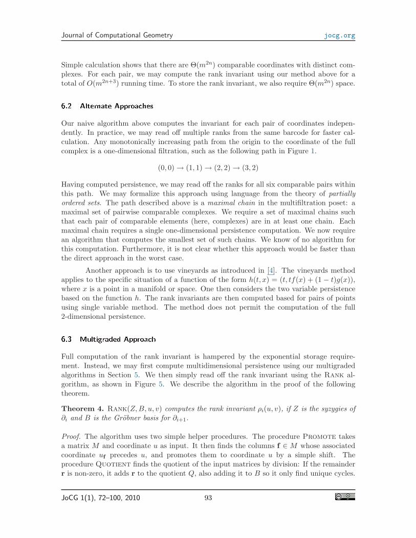
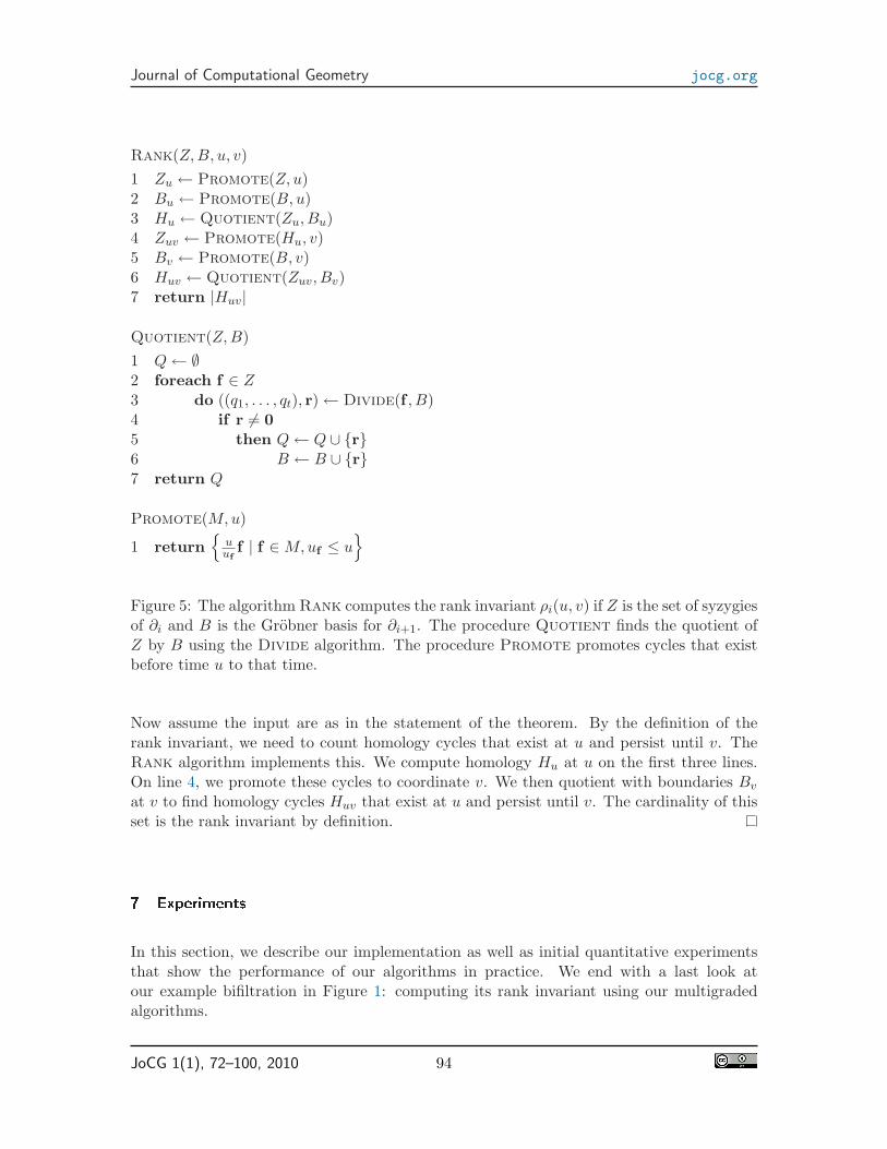
Full computation of the rank invariant is hampered by the exponential storage require-ment. Instead, we may first compute multidimensional persistence using our multigradedalgorithms in Section 5. We then simply read off the rank invariant using the Rank al-gorithm, as shown in Figure 5. We describe the algorithm in the proof of the followingtheorem.

Theorem 4. Rank(Z, B, u, v) computes the rank invariant ρi(u, v), if Z is the syzygies of∂i and B is the Grobner basis for ∂i+1.

Proof. The algorithm uses two simple helper procedures. The procedure Promote takesa matrix M and coordinate u as input. It then finds the columns f ∈ M whose associatedcoordinate uf precedes u, and promotes them to coordinate u by a simple shift. Theprocedure Quotient finds the quotient of the input matrices by division: If the remainderr is non-zero, it adds r to the quotient Q, also adding it to B so it only find unique cycles.

JoCG 1(1), 72–100, 2010 93

Journal of Computational Geometry jocg.org

Rank(Z, B, u, v)

1 Zu ← Promote(Z, u)2 Bu ← Promote(B, u)3 Hu ← Quotient(Zu, Bu)4 Zuv ← Promote(Hu, v)5 Bv ← Promote(B, v)6 Huv ← Quotient(Zuv, Bv)7 return |Huv|

Quotient(Z, B)

1 Q← ∅2 foreach f ∈ Z3 do ((q1, . . . , qt), r)← Divide(f , B)4 if r 6= 0

5 then Q← Q ∪ {r}6 B ← B ∪ {r}7 return Q

Promote(M, u)

1 return{

uuf

f | f ∈M, uf ≤ u}

Figure 5: The algorithm Rank computes the rank invariant ρi(u, v) if Z is the set of syzygiesof ∂i and B is the Grobner basis for ∂i+1. The procedure Quotient finds the quotient ofZ by B using the Divide algorithm. The procedure Promote promotes cycles that existbefore time u to that time.

Now assume the input are as in the statement of the theorem. By the definition of therank invariant, we need to count homology cycles that exist at u and persist until v. TheRank algorithm implements this. We compute homology Hu at u on the first three lines.On line 4, we promote these cycles to coordinate v. We then quotient with boundaries Bv

at v to find homology cycles Huv that exist at u and persist until v. The cardinality of thisset is the rank invariant by definition.

7 Experiments

In this section, we describe our implementation as well as initial quantitative experimentsthat show the performance of our algorithms in practice. We end with a last look atour example bifiltration in Figure 1: computing its rank invariant using our multigradedalgorithms.

JoCG 1(1), 72–100, 2010 94

Journal of Computational Geometry jocg.org

7.1 Implementation

We initially used software packages CoCoA[3] and Macaulay [11], which contain standardimplementations of the algorithms. These packages were immensely helpful during oursoftware development as they allowed for quick and convenient testing of the basic algo-rithms. In practice, there are two problems in using these packages for large datasets.First, these packages are slow since they are general and not customized for homogeneousmatrices. Second, these packages produce verbose output that must be parsed for furthercomputation.

Our experience led us to implement our algorithms for computation over Z2, opti-mizing the code for this field. Our implementation is in Java and and was tested underMac OS X 10.5.6 running on a 2.3 Ghz Intel Quad-Core Xeon MacPro computer with 6 GBRAM.

7.2 Data

We generate n × n, random, bifiltered, homogeneous matrices, to simulate the boundarymatrix ∂k−1 of a random bifiltered complex with n simplices in dimensions k− 1 and k− 2.We use the following procedure:

1. Randomly generate n monomials {m1, . . . , mn} corresponding to the monomials as-sociated with the basis elements of the rows.

2. For each column f generate k integers indexing the non-zero rows.

3. Set the column monomial to be lcm(mj), where {mj}j are the monomials of rowswith non-zero

Each column in this matrix has k non-zero elements and is homogeneous by construction.We also generate random matrices but limit the number of unique monomials in the matrixto be O(h2) for different values of h. The basic idea behind these tests is that the range ofthe filtrations in a cell complex can typically be divided into smaller discrete intervals. Forgeneration, we replace the first step of the procedure above with the following two steps:

0. Randomly generate h unique monomials {l1, . . . , lh}.

1. Generate n monomials {m1, . . . , mn} corresponding to the monomials associated withthe basis elements of the rows such that mi ∈ {l1, . . . , lh}.

After executing step 2 and 3 above, our resulting matrix has homogeneous columns with knon-zero elements and at most h2 unique monomials.

7.3 Size & Timings

According to Lemma 4, the number of columns in the Grobner basis for a random matrixmay grow O(n3) as we have n = m here. Figure 6(a) shows that the growth of the Grobner

JoCG 1(1), 72–100, 2010 95

Journal of Computational Geometry jocg.org

102

103

104

105

102

103

104

|G|

n

k = 2k = 4

(a) |G|

10-3

10-2

10-1

100

101

102

103

104

105

102

103

104

Tim

e (

s)

n

k = 2 (l)k = 2 (m)

k = 4 (l)k = 4 (m)

(b) Time

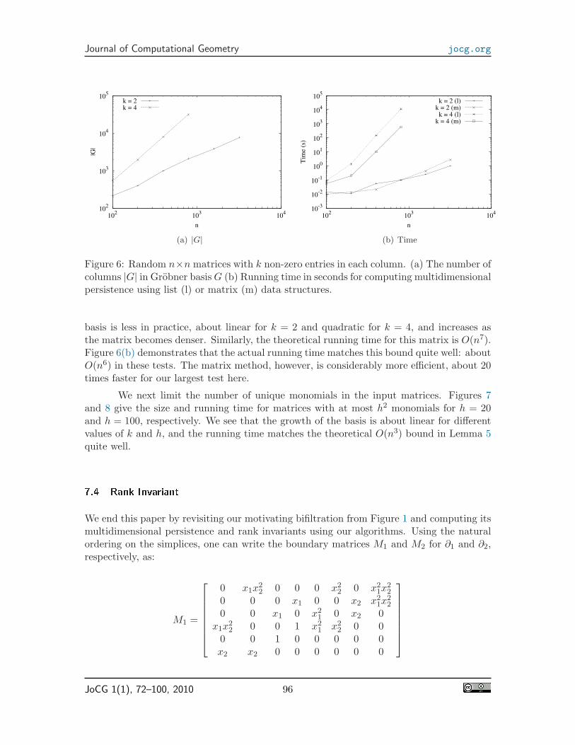
Figure 6: Random n×n matrices with k non-zero entries in each column. (a) The number ofcolumns |G| in Grobner basis G (b) Running time in seconds for computing multidimensionalpersistence using list (l) or matrix (m) data structures.

basis is less in practice, about linear for k = 2 and quadratic for k = 4, and increases asthe matrix becomes denser. Similarly, the theoretical running time for this matrix is O(n7).Figure 6(b) demonstrates that the actual running time matches this bound quite well: aboutO(n6) in these tests. The matrix method, however, is considerably more efficient, about 20times faster for our largest test here.

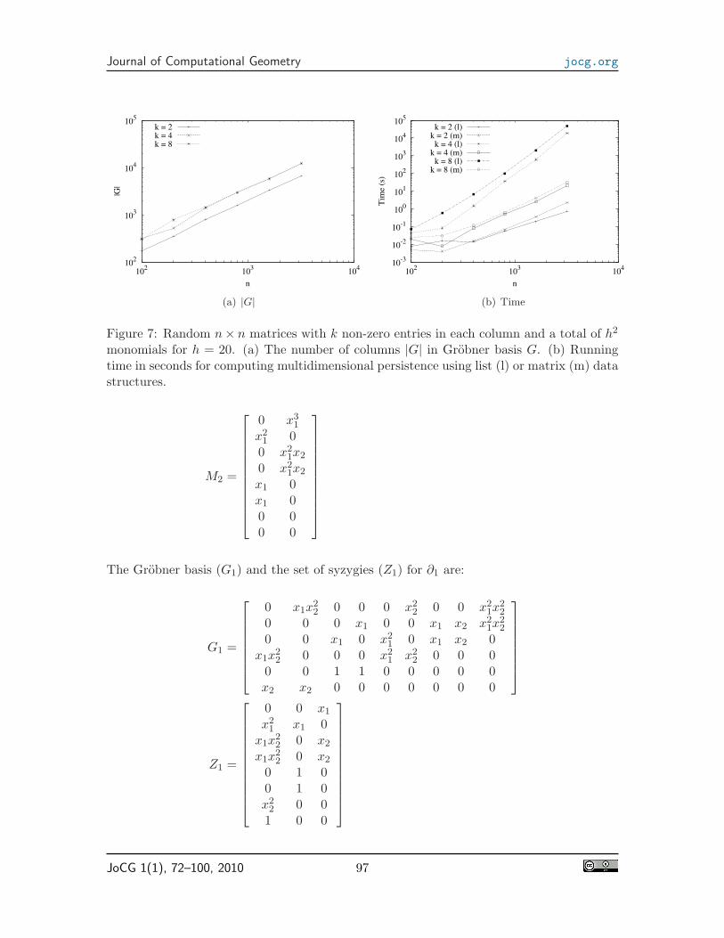
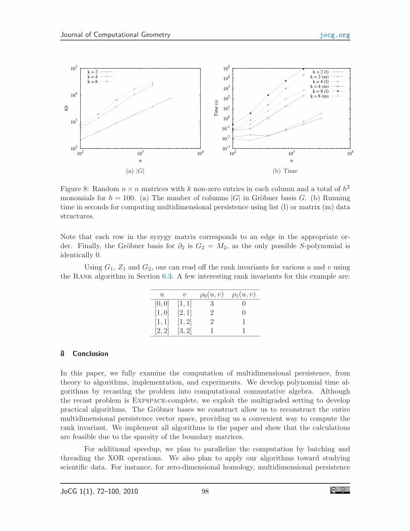
We next limit the number of unique monomials in the input matrices. Figures 7and 8 give the size and running time for matrices with at most h2 monomials for h = 20and h = 100, respectively. We see that the growth of the basis is about linear for differentvalues of k and h, and the running time matches the theoretical O(n3) bound in Lemma 5quite well.

7.4 Rank Invariant

We end this paper by revisiting our motivating bifiltration from Figure 1 and computing itsmultidimensional persistence and rank invariants using our algorithms. Using the naturalordering on the simplices, one can write the boundary matrices M1 and M2 for ∂1 and ∂2,respectively, as:

M1 =

0 x1x22 0 0 0 x2

2 0 x21x

22

0 0 0 x1 0 0 x2 x21x

22

0 0 x1 0 x21 0 x2 0

x1x22 0 0 1 x2

1 x22 0 0

0 0 1 0 0 0 0 0x2 x2 0 0 0 0 0 0

JoCG 1(1), 72–100, 2010 96

Journal of Computational Geometry jocg.org

102

103

104

105

102

103

104

|G|

n

k = 2k = 4k = 8

(a) |G|

10-3

10-2

10-1

100

101

102

103

104

105

102

103

104

Tim

e (

s)

n

k = 2 (l)k = 2 (m)

k = 4 (l)k = 4 (m)

k = 8 (l)k = 8 (m)

(b) Time

Figure 7: Random n× n matrices with k non-zero entries in each column and a total of h2

monomials for h = 20. (a) The number of columns |G| in Grobner basis G. (b) Runningtime in seconds for computing multidimensional persistence using list (l) or matrix (m) datastructures.

M2 =

0 x31

x21 00 x2

1x2

0 x21x2

x1 0x1 00 00 0

The Grobner basis (G1) and the set of syzygies (Z1) for ∂1 are:

G1 =

0 x1x22 0 0 0 x2

2 0 0 x21x

22

0 0 0 x1 0 0 x1 x2 x21x

22

0 0 x1 0 x21 0 x1 x2 0

x1x22 0 0 0 x2

1 x22 0 0 0

0 0 1 1 0 0 0 0 0x2 x2 0 0 0 0 0 0 0

Z1 =

0 0 x1

x21 x1 0

x1x22 0 x2

x1x22 0 x2

0 1 00 1 0x2

2 0 01 0 0

JoCG 1(1), 72–100, 2010 97

Journal of Computational Geometry jocg.org

102

103

104

105

102

103

104

|G|

n

k = 2k = 4k = 8

(a) |G|

10-3

10-2

10-1

100

101

102

103

104

105

102

103

104

Tim

e (

s)

n

k = 2 (l)k = 2 (m)

k = 4 (l)k = 4 (m)

k = 8 (l)k = 8 (m)

(b) Time

Figure 8: Random n× n matrices with k non-zero entries in each column and a total of h2

monomials for h = 100. (a) The number of columns |G| in Grobner basis G. (b) Runningtime in seconds for computing multidimensional persistence using list (l) or matrix (m) datastructures.

Note that each row in the syzygy matrix corresponds to an edge in the appropriate or-der. Finally, the Grobner basis for ∂2 is G2 = M2, as the only possible S-polynomial isidentically 0.

Using G1, Z1 and G2, one can read off the rank invariants for various u and v usingthe Rank algorithm in Section 6.3. A few interesting rank invariants for this example are:

u v ρ0(u, v) ρ1(u, v)

[0, 0] [1, 1] 3 0[1, 0] [2, 1] 2 0[1, 1] [1, 2] 2 1[2, 2] [3, 2] 1 1

8 Con lusion

In this paper, we fully examine the computation of multidimensional persistence, fromtheory to algorithms, implementation, and experiments. We develop polynomial time al-gorithms by recasting the problem into computational commutative algebra. Althoughthe recast problem is Expspace-complete, we exploit the multigraded setting to developpractical algorithms. The Grobner bases we construct allow us to reconstruct the entiremultidimensional persistence vector space, providing us a convenient way to compute therank invariant. We implement all algorithms in the paper and show that the calculationsare feasible due to the sparsity of the boundary matrices.

For additional speedup, we plan to parallelize the computation by batching andthreading the XOR operations. We also plan to apply our algorithms toward studyingscientific data. For instance, for zero-dimensional homology, multidimensional persistence

JoCG 1(1), 72–100, 2010 98

Journal of Computational Geometry jocg.org

corresponds to clustering multiparameterized data, This fresh perspective, as well as a newarsenal of computational tools, allows us to attack an old and significant problem in dataanalysis.

Referen es

[1] G. Carlsson, T. Ishkhanov, V. de Silva, and A. Zomorodian. On the local behavior ofspaces of natural images. International Journal of Computer Vision, 76(1):1–12, 2008.

[2] G. Carlsson and A. Zomorodian. The theory of multidimensional persistence. Discrete& Computational Geometry, 42(1):71–93, 2009.

[3] CoCoATeam. CoCoA: a system for doing Computations in Commutative Algebra.http://cocoa.dima.unige.it.

[4] D. Cohen-Steiner, H. Edelsbrunner, and D. Morozov. Vines and vineyards by updatingpersistence in linear time. In Proc. ACM Symposium on Computational Geometry,pages 119 – 126, 2006.

[5] A. Collins, A. Zomorodian, G. Carlsson, and L. Guibas. A barcode shape descriptorfor curve point cloud data. Computers and Graphics, 28:881–894, 2004.

[6] D. A. Cox, J. Little, and D. O’Shea. Using algebraic geometry, volume 185 of GraduateTexts in Mathematics. Springer, New York, second edition, 2005.

[7] V. de Silva, R. Ghrist, and A. Muhammad. Blind swarms for cov-erage in 2-D. In Proceedings of Robotics: Science and Systems, 2005.http://www.roboticsproceedings.org/rss01/.

[8] H. Edelsbrunner, D. Letscher, and A. Zomorodian. Topological persistence and sim-plification. Discrete & Computational Geometry, 28:511–533, 2002.

[9] S. Eilenberg and J. A. Zilber. Semi-simplicial complexes and singular homology. Annalsof Mathematics, 51(3):499–513, 1950.

[10] P. Frosini and M. Mulazzani. Size homotopy groups for computation of natural sizedistances. Bull. Belg. Math. Soc. Simon Stevin, 6(3):455–464, 1999.

[11] D. R. Grayson and M. E. Stillman. Macaulay 2, a software system for research inalgebraic geometry. http://www.math.uiuc.edu/Macaulay2/.

[12] A. Gyulassy, V. Natarajan, V. Pascucci, P. T. Bremer, and B. Hamann. Topology-basedsimplification for feature extraction from 3D scalar fields. In Proc. IEEE Visualization,pages 275–280, 2005.

[13] A. Hatcher. Algebraic Topology. Cambridge University Press, New York, NY, 2002.http://www.math.cornell.edu/~hatcher/AT/ATpage.html.

JoCG 1(1), 72–100, 2010 99

Journal of Computational Geometry jocg.org

[14] T. Kaczynski, K. Mischaikow, and M. Mrozek. Computational Homology. Springer-Verlag, New York, NY, 2004.

[15] M. Levoy and P. Hanrahan. Light field rendering. In Proc. SIGGRAPH, pages 31–42,1996.

[16] Y. Matsumoto. An Introduction to Morse Theory, volume 208 of Iwanami Series inModern Mathematics. American Mathematical Society, Providence, RI, 2002.

[17] E. W. Mayr. Some complexity results for polynomial ideals. Journal of Complexity,13(3):303–325, 1997.

[18] G. Singh, F. Memoli, T. Ishkhanov, G. Sapiro, G. Carlsson, and D. L. Ringach. Topo-logical analysis of population activity in visual cortex. Journal of Vision, 8(8):1–18, 62008.

[19] G. Turk and M. Levoy. Zippered polygon meshes from range images. In Proc. SIG-GRAPH, pages 311–318, 1994.

[20] J. von zur Gathen and J. Gerhard. Modern Computer Algebra. Cambridge UniversityPress, Cambridge, UK, second edition, 2003.

[21] F. Zhao and L. J. Guibas. Wireless Sensor Networks: An Information ProcessingApproach. Morgan-Kaufmann, San Francisco, CA, 2004.

[22] A. Zomorodian. Computational topology. In M. Atallah and M. Blanton, editors,Algorithms and Theory of Computation Handbook, volume 2, chapter 3. Chapman &Hall/CRC Press, Boca Raton, FL, second edition, 2010.

[23] A. Zomorodian and G. Carlsson. Computing persistent homology. Discrete & Compu-tational Geometry, 33(2):249–274, 2005.

JoCG 1(1), 72–100, 2010 100