TECHNICAL REPORT R-190 1992

UNIVERSITY OF CALIFORNIA Los Angeles

Qualitative Probabilities: A Normative Framework for Commonsense

"R • _._"easoning

A dissertation submitted in partial satisfaction of the requirements for the degree

Doctor of Philosophy in Computer Science

by

Moises Goldszmidt

1992

Report Documentation Page Form ApprovedOMB No. 0704-0188

Public reporting burden for the collection of information is estimated to average 1 hour per response, including the time for reviewing instructions, searching existing data sources, gathering andmaintaining the data needed, and completing and reviewing the collection of information Send comments regarding this burden estimate or any other aspect of this collection of information,including suggestions for reducing this burden, to Washington Headquarters Services, Directorate for Information Operations and Reports, 1215 Jefferson Davis Highway, Suite 1204, ArlingtonVA 22202-4302 Respondents should be aware that notwithstanding any other provision of law, no person shall be subject to a penalty for failing to comply with a collection of information if itdoes not display a currently valid OMB control number

1. REPORT DATE 1992 2. REPORT TYPE

3. DATES COVERED 00-00-1992 to 00-00-1992

4. TITLE AND SUBTITLE Qualitative Probabilities: A Normative Framework for Commonsense Reasoning

5a. CONTRACT NUMBER

5b. GRANT NUMBER

5c. PROGRAM ELEMENT NUMBER

6. AUTHOR(S) 5d. PROJECT NUMBER

5e. TASK NUMBER

5f. WORK UNIT NUMBER

7. PERFORMING ORGANIZATION NAME(S) AND ADDRESS(ES) University of California Los Angeles,Department of ComputerScience,Los Angeles,CA,90095

8. PERFORMING ORGANIZATIONREPORT NUMBER

9. SPONSORING/MONITORING AGENCY NAME(S) AND ADDRESS(ES) 10. SPONSOR/MONITOR’S ACRONYM(S)

11. SPONSOR/MONITOR’S REPORT NUMBER(S)

12. DISTRIBUTION/AVAILABILITY STATEMENT Approved for public release; distribution unlimited

13. SUPPLEMENTARY NOTES

14. ABSTRACT Intelligent agents are expected to generate plausible predictions and explanations in partially unknown andhighly dynamic environments. Thus, they should be able to retract old conclusions in light of new evidenceand to efficiently manage wide fluctuations of uncertainty. Neither mathematical logic nor numericalprobability fully accommodates these requirements. In this dissertation I propose a formalism thatfacilitates reasoning with qualitative rules, facts, and deductively closed beliefs (as in logic), yet permits usto retract beliefs in response to changing contexts and imprecise observations (as in probability). Domainknowledge is encoded as if-then rules admitting exceptions with different degrees of abnormality, andqueries specify contexts with different levels of precision. I develop effective procedures for testing theconsistency of such knowledge bases and for computing whether (and to what degree) a given query isconfirmed or denied. These procedures require a polynomial number of propositional satisfiability testsand hence are tractable for Horn expressions. Finally, I show how to give rules causal character byenforcing a Markovian condition of independence. The resulting formalism provides the necessarymachinery for embodying belief updates and belief revision, generating explanations, and reasoning aboutactions and change.

15. SUBJECT TERMS

16. SECURITY CLASSIFICATION OF: 17. LIMITATION OF ABSTRACT Same as

Report (SAR)

18. NUMBEROF PAGES

174

19a. NAME OFRESPONSIBLE PERSON

a REPORT unclassified

b ABSTRACT unclassified

c THIS PAGE unclassified

Standard Form 298 (Rev. 8-98) Prescribed by ANSI Std Z39-18

@ Copyright by Moises Goldszmidt

1992

The dissertation of Moises Goldszmidt is approved.

Kit Fine

Yiannis Moschovakis

D. Stott Parker

Sheila A. Greibach

Judea Pearl, Committee Chair

University of California, Los Angeles

1992

li

TABLE OF CONTENTS

1 Introduction ................. .

1.1 Overview and Summary of Contributions

1.2 Extensional and Conditional Approaches

1.2.1 Reiter's Default Logic

1.2.2 McCarthy's Circumscription

1.2.3 Moore's Autoepistemic Logic

2 The Consistency of Conditional Knowledge Bases

2.1 Introduction ............. .

2.2 Notation and Preliminary Definitions

2.3 Probabilistic Consistency and Entailment .

2.4 An Effective Procedure for Testing Consistency

2.5 Examples . . . . . . . . . . . . . . . . . . . . .

2.6 Reasoning with p-Inconsistent Knowledge Bases

2. 7 Discussion . . . . . . . . . . . . . . . . . . . . .

3 Plausibility I: A Maximum Entropy Approach

3.1 Introduction ............... .

3.2 Parameterized Probability Distributions

3.3 Plausible Conclusions and Maximum Entropy

3.4 Examples . . . . . . . .

3.5 Non-Minimal-Core Sets .

3.6 Discussion ....... .

1

4

7

9

10

12

14

14

18

19

23

25

28

32

36

36

38

42

48

51

53

4 Plausibility II: System-z+ . . . . . . . . . . . . . . . . . . . . . . 56

4.1 Rankings as an Order-of-Magnitude Abstraction of Probabilities 56

4.2 Preliminary Definitions: Rankings Revisited 60

4.3 Plausible Conclusions: The z+ -Rank 63

4.4 Examples . . . . . . . . . . . . . . .

4.5 Belief Change, Soft Evidence, and Imprecise Observations

111

68

70

4.6

4.7

4.5.1 Type-J: All Things Considered ..... .

4.5.2 Type-1 Reports: Nothing Else Considered

4.5.3 Complexity Analysis . . . . . . . . . . .

Relation to the AGM Theory of Belief Revision

Discussion

5 Causality . . .

5.1 Introduction

5.2 Stratified Rankings

5.3 c-Entailment ....

c- Consistency 5.3.1

5.3.2 Accountability: A Framework For Explanations

5.3.3 The most normal stratified ranking

5.4 Belief Update ............. .

5.4.1 The dynamics of belief update .

5.4.2 Relation to KM postulates

5.4.3 Related work

5.5 Discussion . . . . .

6 Concluding Remarks

6.1 Summary ..

6.2 Future Work .

6.2.1 Semantical Extensions

6.2.2 Qualitative and Quantitative Information .

6.2.3 Learning .................. .

A Proofs

B The Lagrange Multipliers Technique.

References . . . . . . . . . . . . . . . . . . .

IV

72

73

75

76

80

84

84

86

90

96

97

102

104

107

109

111

112

115

115

116

116

117

118

119

142

143

LIST OF FIGURES

1.1 Schematic of the system proposed. 2

2.1 An effective procedure for testing consistency in O(IDI 2 + lSI) propositional satisfiability tests. . . . . . . . . . . . . . . . . . . . 23

3.1 Procedure for computing the Z* -ordering on rules .. 47

4.1 Consistency and rankings. . . . . . . . . . . . . . . 62

4.2 Procedure for computing the z+ -ordering on rules. 65

5.1 Underlying graph for the causal rules in the battery example 87

5.2 Stratification condition. . . . . . . . . . . . . . . . . . . . . . 88

5.3 The noisy-or interaction model: C1 , ... , Cn are the set of causes for E, and each Ji represents an inhibitor or abnormality for Ci ---t E 99

5.4 A Schematic view of the car example. . . . . . . . . . . .

5.5 Graph depicting the causal dependencies in Example .5.3

v

100

106

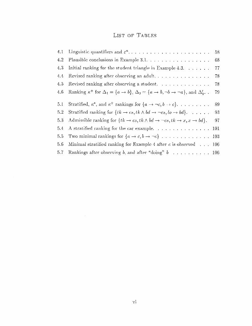
LIST OF TABLES

4.1 Linguistic quantifiers and c;n. . . . . . 58

4.2 Plausible conclusions in Example 3.1. 68

4.3 Initial ranking for the student triangle in Example 4.3. 77

4.4 Revised ranking after observing an adult. . 78

4.5 Revised ranking after observing a student. 78

4.6 Ranking 1\:+ for .6.1 = {a -t b}, .6.2 = {a -t b, -.b -t -.a}, and .6.~. 79

5.1 Stratified, fi:*, and 1\:+ rankings for {a -t -.c, b -t c}. . . . 89

5.2 Stratified ranking for { tk -t cs, tk 1\ bd -t -.cs, lo-t bd}. 93

5.3 Admissible ranking for { tk -t cs, tk 1\ bd -t -.cs, tk -t x, x -t bd}. 97

5.4 A stratified ranking for the car example. . 101

5.5 Two minimal rankings for {a -t c, b -t -.c} 103

5.6 Minimal stratified ranking for Example 4 after cis observed 106

5.7 Rankings after observing b, and after "doing" b . . . . . . . 106

Vl

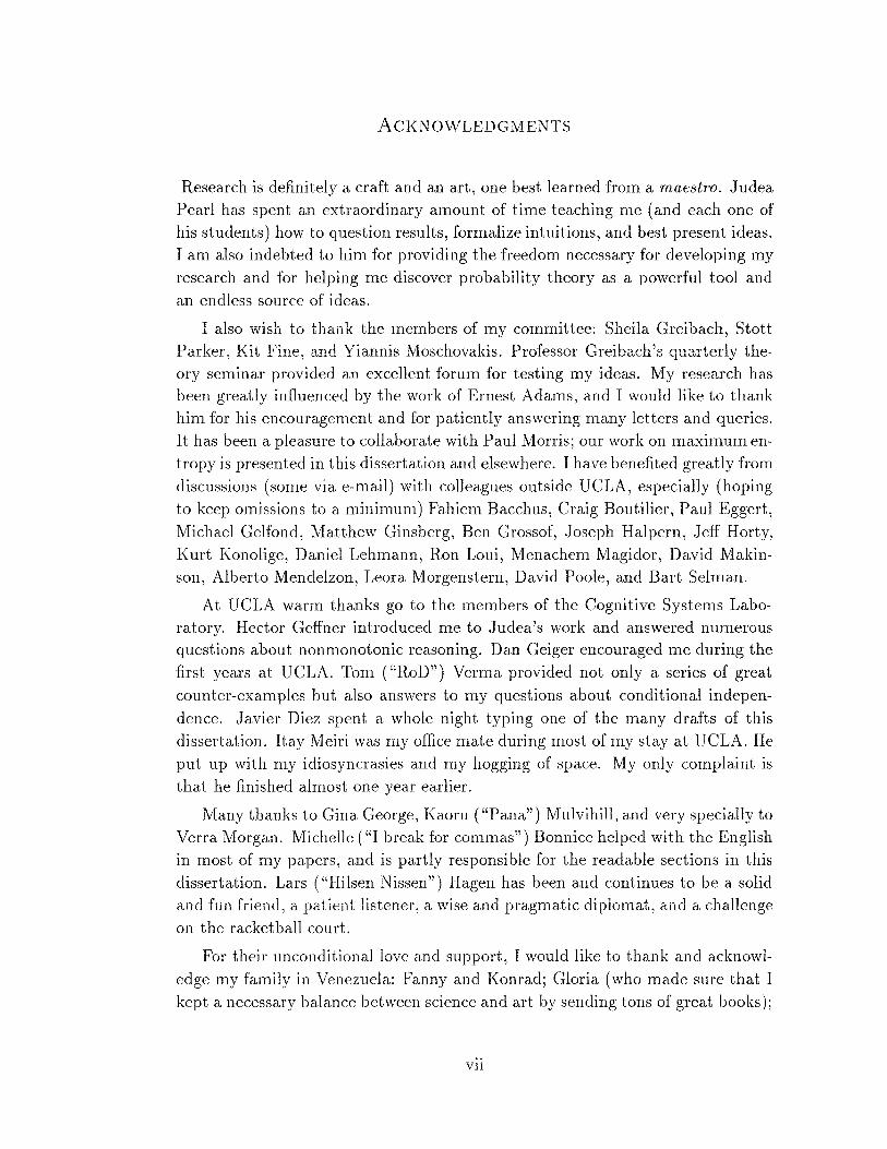
ACKNOWLEDGMENTS

Research is definitely a craft and an art, one best learned from a maestro. Judea Pearl has spent an extraordinary amount of time teaching me (and each one of his students) how to question results, formalize intuitions, and best present ideas. I am also indebted to him for providing the freedom necessary for developing my research and for helping me discover probability theory as a powerful tool and an endless source of ideas.

I also wish to thank the members of my committee: Sheila Greibach, Stott Parker, Kit Fine, and Yiannis Moschovakis. Professor Greibach's quarterly the­ory seminar provided an excellent forum for testing my ideas. My research has been greatly influenced by the work of Ernest Adams, and I would like to thank him for his encouragement and for patiently answering many letters and queries. It has been a pleasure to collaborate with Paul Morris; our work on maximum en­tropy is presented in this dissertation and elsewhere. I have benefited greatly from discussions (some via e-mail) with colleagues outside UCLA, especially (hoping to keep omissions to a minimum) Fahiem Bacchus, Craig Boutilier, Paul Eggert, Michael Gelfand, Matthew Ginsberg, Ben Grossof, Joseph Halpern, Jeff Horty, Kurt Konolige, Daniel Lehmann, Ron Loui, Menachem Magidor, David Makin­son, Alberto Mendelzon, Leora Morgenstern, David Poole, and Bart Selman.

At UCLA warm thanks go to the members of the Cognitive Systems Labo­ratory. Hector Geffner introduced me to Judea's work and answered numerous questions about nonmonotonic reasoning. Dan Geiger encouraged me during the first years at UCLA. Tom ("RoD") Verma provided not only a series of great counter-examples but also answers to my questions about conditional indepen­dence. Javier Diez spent a whole night typing one of the many drafts of this dissertation. Itay Meiri was my office mate during most of my stay at UCLA. He put up with my idiosyncrasies and my hogging of space. My only complaint is that he finished almost one year earlier.

Many thanks to Gina George, Kaoru ("Pana") Mulvihill, and very specially to Verra Morgan. Michelle ("I break for commas") Bonnice helped with the English in most of my papers, and is partly responsible for the readable sections in this dissertation. Lars ( "Hilsen Nissen") Hagen has been and continues to be a solid and fun friend, a patient listener, a wise and pragmatic diplomat, and a challenge on the racketball court.

For their unconditional love and support, I would like to thank and acknowl­edge my family in Venezuela: Fanny and Konrad; Gloria (who made sure that I kept a necessary balance between science and art by sending tons of great books);

Vll

my grandparents, Dora and Paul, Enja and Isaac; my brothers and sisters, Freddy, Helen, Alexandra (in Italy), Leon, William and Ricardo. My deepest gratitude goes to my parents, Ada and Albert, for believing in me, always being there, making things possible, and constantly proving that nothing comes before the well-being of their children.

Almost every memory of happiness from my childhood is laced with the mu­sical voice and laughter of my grandmother, Dora, who passed away during the summer of 1990. She is the only reason that would make me want to believe in heaven. Abuela Dora, I miss you.

Tania - best friend, compinche, and my beautiful wife - has the miraculous ability to turn worry into fun. She has encouraged and participated in every one of my (big and small) projects and has been an uncompromising critic of my work (and my music). Tania I love you. Thanks!

The music is by Charles Mingus.

The funding is by an IBM Graduate Fellowship 1990-1992, and by NSF grant #IRI-9200918, AFOSR grant #900136, and MICRO grant #91-124.

Vlll

1960

1983

1983-1985

1985-1986

1986-1987

1987

1987-1992

1990-1992

1992

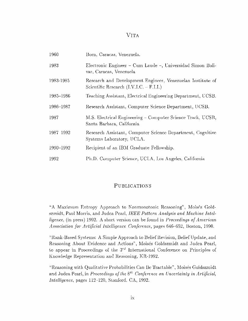
VITA

Born, Caracas, Venezuela.

Electronic Engineer - Cum Laude -, Universidad Simon Boli­var, Caracas, Venezuela

Research and Development Engineer, Venezuelan Institute of Scientific Research (I.V.I.C. F.I.I.)

Teaching Assistant, Electrical Engineering Department, UCSB.

Research Assistant, Computer Science Department, UCSB.

M.S. Electrical Engineering- Computer Science Track, UCSB, Santa Barbara, California

Research Assistant, Computer Science Department, Cognitive Systems Laboratory, UCLA.

Recipient of an IBM Graduate Fellowship.

Ph.D. Computer Science, UCLA, Los Angeles, California

PUBLICATIONS

"A Maximum Entropy Approach to Nonmonotonic Reasoning", Moises Gold­szmidt, Paul Morris, and Judea Pearl, IEEE Pattern Analysis and Machine Intel­

ligence, (in press) 1992. A short version can be found in Proceedings of American

Association for Artificial Intelligence Conference, pages 646-652, Boston, 1990.

"Rank-Based Systems: A Simple Approach to Belief Revision, Belief Update, and Reasoning About Evidence and Actions", Moises Goldszmidt and Judea Pearl, to appear in Proceedings of the 3rd International Conference on Principles of Knowledge Representation and Reasoning, KR-1992.

"Reasoning with Qualitative Probabilities Can Be Tractable", Moises Goldszmidt and Judea Pearl, in Proceedings of the 8th Conference on Uncertainty in Artificial)

Intelligence, pages 112-120, Stanford, CA, 1992.

IX

"Stratified Rankings for Causal Modeling", Moises Goldszmidt and Judea Pearl, in Proceedings of the Fourth International Workshop on Nonmonotonic Reason­

ing, pages 99-110, Vermont, 1992.

"On The Consistency of Defeasible Databases", Moises Goldszmidt and Judea Pearl, Artificial Intelligence, Vol. .52:2, pages 121-149, 1991.

"System z+: A Formalism for Reasoning with Variable Strength Defaults", Moises Goldszmidt and Judea Pearl, in Proceedings of American Association for Artificial Intelligence Conference, pages 399-404, Anaheim, CA, 1991.

"On The Relation Between Rational Closure and System-Z", Moises Goldszmidt and Judea Pearl, in Third International Workshop on Nonmonotonic Reasoning,

pages 130-140, South Lake Tahoe, CA, 1990.

"Deciding Consistency of Databases Containing Defeasible and Strict Informa­tion", Moises Goldszmidt and Judea Pearl, in M. Henrion et. al, editor, Uncer­

tainty in Artificial Intelligence (Vol. 5). North Holland, Amsterdam, 1990. Also in the UCLA Annual Research Review 1990.

X

ABSTRACT OF THE DISSERTATION

Qualitative Probabilities: A Normative Framework for Commonsense

Reasoning

by

Moises Goldszmidt Doctor of Philosophy in Computer Science University of California, Los Angeles, 1992

Professor Judea Pearl, Chair

Intelligent agents are expected to generate plausible predictions and explanations in partially unknown and highly dynamic environments. Thus, they should be able to retract old conclusions in light of new evidence and to efficiently man­age wide fluctuations of uncertainty. Neither mathematical logic nor numerical probability fully accommodates these requirements.

In this dissertation I propose a formalism that facilitates reasoning with qual­itative rules, facts, and deductively closed beliefs (as in logic), yet permits us to

retract beliefs in response to changing contexts and imprecise observations (as in probability). Domain knowledge is encoded as if-then rules admitting exceptions

with different degrees of abnormality, and queries specify contexts with different levels of precision. I develop effective procedures for testing the consistency of such knowledge bases and for computing whether (and to what degree) a given query is confirmed or denied. These procedures require a polynomial number

of propositional satisfiability tests and hence are tractable for Horn expressions. Finally, I show how to give rules causal character by enforcing a Markovian condi­

tion of independence. The resulting formalism provides the necessary machinery for embodying belief updates and belief revision, generating explanations, and reasoning about actions and change.

XI

CHAPTER 1

Introduction

In their everyday interactions with the world, people continuously jump to con­clusions on the basis of imperfect and defeasible information. For example, we

normally expect to find our car where we parked it last, and upon turning the ignition key, we expect the engine to start. These expectations are plausible but not provable from what is known at the time they are assessed, and they may be replaced as new evidence is encountered. A stolen car will not be where we parked it last. An engine with a dead battery will not start. Yet, despite the multitude of possible scenarios, people operate under a fairly uniform consensus

as to what is plausible, that is, what should be upheld as true for practical pur­poses. This suggests that there are simple principles that govern the dynamics of plausible reasoning, including the distinction between plausible and implausible conclusions.

This dissertation is concerned with casting the principles governing plausible reasoning in a formal language. vVe wish to create through such formalization programs capable both of accepting and organizing input ranging from defeasible information such as "typically, if we turn the car's ignition the engine starts"

to nondefeasible (strict) information such as "all humans are mortal" and of an­

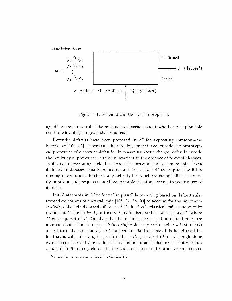
swering queries about what would be a plausible conclusion given some particular context. Figure 1.1 presents a schematic of this project. The set of "if !..pi then

'l/Ji'' rules, !..pi ~ 'l/Ji, represents a knowledge base encoding information about the world. The incompleteness of this information is modeled by allowing exceptions to these rules, where /5i represents the degree of abnormality of these exceptions. Rules expressing what is normally the case without excluding the possibility of exceptions, are commonly known in Artificial Intelligence (AI) as default rules.l

A query is a pair ( </J, (]') representing the context <f and the target (]'. The con­

text of a query contains factual information on what is currently known about the environment, which may originate from either passive observations or ac­tive manipulations. 2 The target (]' is a propositional hypothesis representing the

1 In the database literature, these rules play the role of integrity constraints, but are normally treated as hard laws, tolerating no exceptions [111].

2This distinction is of crucial importance, as shown in Section 5.4.

1

Knowledge Base:

Confirmed

~= 1-----+- 0' (degree?)

Denied

¢: Actions - Observations Query: ( ¢, 0')

Figure 1.1: Schematic of the system proposed.

agent's current interest. The output is a decision about whether 0' is plausible (and to what degree) given that ¢ is true.

Recently, defaults have been proposed in AI for expressing commonsense knowledge [109, 45]. Inheritance hierarchies, for instance, encode the prototypi­cal properties of classes as defaults. In reasoning about change, defaults encode the tendency of properties to remain invariant in the absence of relevant changes. In diagnostic reasoning, defaults encode the rarity of faulty components. Even deductive databases usually embed default "closed-world" assumptions to fill in missing information. In short, any activity for which we cannot afford to spec­ify in advance all responses to all conceivable situations seems to require use of defaults.

Initial attempts in AI to formalize plausible reasoning based on default rules favored extensions of classical logic [108, 87, 88, 90] to account for the non mono­tonicity of the default-based inferences.3 Deduction in classical logic is monotonic: given that C is entailed by a theory T, C is also entailed by a theory T', where T' is a superset ofT. On the other hand, inferences based on default rules are nonmonotonic: For example, I believe/infer that my car's engine will start (C) once I turn the ignition key (T), but would like to retract this belief (and in­fer that it will not start, i.e., --,C) if the battery is dead (T'). i1Jthough these extensions successfully reproduced this nonmonotonic behavior, the interactions among defaults rules yield conflicting and sometimes couterintuitive conclusions.

3 These formalisms are reviewed in Section 1.2.

2

For example, consider a knowledge base containing the defaults: "typically pen­guins don't fly", "typically birds fly", and the nondefeasible rule "all penguins are birds". Given that Tweety is a penguin we may conclude that Tweety does not fly based on the information provided by the first default. On the other hand, since Tweety is a penguin, she is also a bird, we may conclude that Tweety flies using the second default rule. The reason we prefer to uphold the conclusion that Tweety does not fly is based on the intuition that defaults providing information about a more specific class of individuals (i.e., penguins in this case) should be considered with a higher priority. There are other cases of default interactions and criteria for avoiding undesirable inferences based on assumptions of minimal

change, and on notions of causality and explanation [57, 36, 8, 45, 121, 54, 118]. Some proposals address the problem of default interactions by asking the user to explicitly specify preferences among rules (e.g., [112, 30, 88, 80]). Ideally, how­ever, such information should be extracted from the rules themselves (or their se­mantical interpretation), since anticipating interactions among defaults becomes increasingly difficult as the size of the knowledge base grows. Furthermore, user

specification of these preferences seems to require a possibly exhaustive enumer­ation of cases, situations, and exceptions, which was precisely what the use of default rules meant to avoid. A related problem is the observation that some plausible conclusions are ha7"deT to retract than others in the face of conflicting evidence. This observation suggests that semantical interpretations of plausible beliefs should involve rankings or orderings among these beliefs (in addition to

truth values) [33, 34, 120].

On the positive side a formalization in terms of a logical framework offers several advantages such as: independence of a specific implementation or do­

main and the possibilities of model theoretic interpretations and well-founded

semantics.

On the other extreme, an alternative to extending classical logic may be prob­ability theory: Uncertainty can be used to represent both the incompleteness of the information in the knowledge base and numbers can be used to model rankings of beliefs. Furthermore, Bayesian conditioning offers a successful and well understood method of dealing with retractions and belief change. Yet, a

straightforward probabilistic interpretation of plausibility in terms of numbers and thresholds will encounter obstacles of its own. First, the picture we form about our environment seems to be encoded in terms of plain beliefs, that is, propositions that are accepted as true (for practical purposes), and continue to guide our actions until refuted by new evidence. These propositions are trans­

mitted linguistically, and are qua.lified by expressions such as such as "generally", "extremely typical", and "very likely", which are void of precise numerical value.

3

Second, plain beliefs also seem to be deductively closed: If~ is believed and 'P is believed, then ~ 1\ 'P is believed as well. Note that if we associate the acceptance of~ as a believed proposition with P( ~) > t, where t is some suitable threshold, it is possible to have both P(~) > t and P('P) > t but P(~ 1\ 'P) < t.

In this thesis, I propose a conditional interpretation of the default rules that presents the merits of both logic and probability. The sentence "if 'P then ~" is interpreted as imposing a preference for accepting ~ over ·~ if 'P is all that is known. This interpretation is based on an abstraction of probability theory

where "if 'P then ~" constrains the conditional probability of ~' given 'P to be infinitesimally close to 1. Intuitively, this amounts to according the consequence ~ a very high likelihood when 'P is all we know.4 As will be seen, at the heart of this formulation is the concept of default priorities, namely, a natural ordering of the rules which is derived automatically from the knowledge base. Repre­senting and reasoning with causal relations is enabled through a stratified set of (probabilistic) independencies based on Markovian considerations. The result is a model-theoretic and semantically vvell-founded account of plausible beliefs that, as in classical logic, are qualitative and deductively closed and, as in probability, are subject to retraction and to varying degrees of firmness.

1.1 Overview and Summary of Contributions

Attaching probabilistic semantics to conditional sentences (i.e., if-then expres­sions) goes back to Adams [1, 2], who developed a logic of indicative conditionals based on infinitesimal probabilities. This logic includes a norm of consistency, called p-consistency, which tolerates exceptions (e.g., "typically, if 'P then ~ and if 'P 1\ '{)1 then ·~") and rules out contradictions (e.g., the pair "typically, if 'P then ~" and "typically, if 'P then ·~"). It also admits a notion of entailment, called p-entailment, which guarantees arbitrarily high probabilities for the con­clusions whenever sufficiently high probabilities can be consistently assigned to the premises.

Unfortunately, Adams' notions of p-consistency and p-entailment were re­stricted to knowledge bases containing only defeasible information. The first contribution of this thesis is the extension of Adams' consistency and entailment to handle both defeasible and strict information (Chap. 2). Strict information is essential for representing definitional or taxonomic information (e.g., "all men are mortal", "penguins are birds"), and incorporating such information into the

4 For a different probabilistic interpretation of the default rules, see Neufeld and Poole [93]. For a statistical interpretation, see the Bacchus (6].

4

knowledge base requires nontrivial changes in the notions of both consistency and entailment. This extension cannot be accomplished by simply treating to the strict conditional ¢> =} r5 as the material implication ¢> :=:> r5. For example, whereas the pair { b :=:> j, b :=:> •f} is logically consistent, the desired semantics should render the set { b =} j, b =} •f} inconsistent. In Chapter 2, I provide a probabilistic semantics for strict conditionals ¢> =} r5 as constraints on admis­sible probability functions forcing the conditional probability of r5 given ¢> to be equal to 1. I then establish effective decision procedures for testing both consis­tency and entailment in knowledge bases containing mixtures of defeasible and strict information. Procedures for reasoning with inconsistent knowledge bases and ways of uncovering the set of rules responsible for the inconsistency are also examined. 5

The second contribution is the formalization and characterization of more powerful notions of entailment (Chaps. 3 and 4). Default reasoning requires two facilities: One forcing retraction of conclusions in light of new refuting evidence (e.g., once vve learn that the battery is dead, we no longer expect the engine to start); the other protecting conclusions from retraction in light of new but irrelevant evidence (e.g., the color of the car should not affect inferences regarding ignition keys, batteries, or engines). p-Entailment excels in the first task, but fails on the second because it is extremely cautious; it only sanctions conclusions that attain high probability in all probability distributions p-consistent with the knowledge base. In order to respect the communication convention that, unless stated explicitly, properties are presumed to be irrelevant to each other, we must consider only distributions that minimize dependencies, that is, they contain only the dependencies that are absolutely implied by the knowledge base (and none

others).

Chapter 3 details an extension of p-entailment where dependencies are mini­mized via the principle of maximum entropy.6 Chapter 3 also provides symbolic procedures for answering queries based on this principle, without the explicit computation of the maximum entropy distribution. A second extension of p­entailment, called system-z+, is presented in Chapter 4. System-z+ restricts the set of probability distributions to those that assign to each model the highest possible likelihood consistent with the default rules. The behavior of these two formalisms is compared and new insights on how semantical features influence the plausibility of the resulting theories are discussed. The approach based on maxi­mum entropy yields more intuitive conclusions in some domains, but system-z+

5The results in this chapter were originally reported in Goldszmidt and Pearl [49]. 6The use of maximum entropy in default reasoning as an extension of p-entailment was

proposed by Pearl in [97].

5

provides considerable computational advantages. An earlier version of Chapter 3 can be found in Goldszmidt et. al. [4 7], while preliminary versions of the results in Chapter 4 were first reported in Goldszmidt and Pearl [50, 53]. These two for­malisms, maximum entropy and system-z+, are completely independent of each other, and Chapter 3 is not a prerequisite for the understanding of Chapter 4.

The third contribution of this thesis is the development of a semantical the­ory and a computational facility for reasoning with variable strength defaults (Sec. 4.3) and soft or imprecise evidence (Sec. 4.5). The capability to reason with variable strength defaults is necessary in domains such as diagnosis, where the analyst may feel strongly that failures are more likely to occur in one type of devices (e.g., multipliers) than in other (e.g., adders). The capability of process­ing soft evidence is important when the context cp (of a query) is not given with absolute certainty, that is, when there is some vague testimony supporting cp but that testimony is undisclosed (or cannot be articulated using the basic proposi­tions in our language, e.g., testimony of the senses) so that only a summary of that testimony saying that "cp is supported to a degree n" can be ascertained.

The introduction of graded defaults and soft evidence requires new query answering machinery which, in the traditional probabilistic setting turned out to be intractable. 7 This thesis shows that the symbolic nature of system-z+ admits a more manageable class of procedures; they require a polynomial number of propositional satisfiability tests and are therefore tractable for Horn expressions.

Augmenting the proposed semantics with the capability to represent causal relations, actions, and reasoning about change is the final contribution of this the­sis (Chap. 5). This is accomplished by invoking the principle of Markov shielding,

which imposes a stratified set of (probabilistic) independences among events. In­formally, the principle can be stated as follows:

Knowing the set of causes for a given effect renders the effect inde­

pendent of all prior events.

I show how the incorporation of this principle gives rise to a norm of consistency, applicable to knowledge bases representing causal relations,8 and how it solves some of the common problems associated with tasks of prediction and explanation reported in the nonmonotonic literature.

7 Most logic-based schemes for default reasoning were also shown to be highly intractable [55] residing in the 2:~ level of the complexity hierarchy, compared with 6.~ in our system.

8 To the best of my knowledge, this is the first consistency criterion devised to ensure the coherence of causal theories.

6

In Section 5.4, I demonstrate how the framework proposed in this dissertation can embody and unify the theories of belief revision (see Alchourr6n, Gardenfors and Makinson [3]) and belief updating (see Katsuno and Mendelzon [65]), two theories of belief change that have been developed independently of research in default reasoning and causal reasoning. Basically, theories of belief change seek general principles for constraining the process by which a rational agent ought to incorporate a new piece of information ¢; into an existing set of beliefs 7/J, regardless of how the two are represented and manipulated. Belief revision deals with information obtained through new observations in a static world, while belief update deals with tracing changes in an evolving world (subjected perhaps to the external influence of actions). 9 I show that both revision and update can be modeled within the same framework using a qualitative version of probabilistic conditioning.

Finally, in Chapter 6 I discuss some open problems and suggest further chal­lenges.

1.2 Extensional and Conditional Approaches

Approaches for formalizing defeasible reasoning can be loosely categorized as either extensional or conditional, depending on the interpretation assigned to the rule cp --t ·¢ .10 Extensional approaches are based on "extending" classical logic by using defaults as rules for augmenting the sets of beliefs in the absence of conflicting evidence (see [87, 108, 89, 90, 45, 109, 38]). These approaches regard the default "if cp then 7/J" as a qualified license believe 7/J given the truth of cp.

Conditional approaches, on the other hand, interpret the same rule as a hard but context dependent constraint to prefer 7/J over •7/J when cp is all that is known (see [36, 38, 69, 74, 23, 101, 14, 49, 50]). Conditional approaches are generally related to conditional logics studied in philosophy.U

As mentioned above, extensional approaches produced systems that exhibit many aspects of nonmonotonicity, thus allowing the retraction of conclusions in light of new information. However, they yield ambiguous results when confronted with conflicting defaults, with no way of distinguishing the intended from the un­intended conclusions (see [112, 57]). In order to impose preferences and prevent generation of undesired inferences, special mechanisms must be devised to permit

9Preliminary versions of this chapter can be found in Goldszmidt and Pearl [54, 52]. 10 Not all formalisms can be categorized as either extensional or conditional. The approach

based on multivalued logics proposed by Ginsberg (46] is one such example. 11 For a survey of conditional logics see [94].

7

the specification of such preferences in the extensional approaches. These include, for example, special nonnorma.l defaults in default logic [30] (see Sec. 1.2.1) and priority-driven minimizations in circumscription [88] (see See. 1.2.2). Such mech­anisms conflict with the original intent of default inference systems, since they require a possibly exhaustive enumeration of the exceptions to each default rule and/or an omniscient user capable of predicting and prioritizing all conceivable interactions among default rules.

In contrast, proposals based on conditional approaches have proven success­ful in enforcing the desired preferences in cases of conflicting defaults (see Ex­amples 2.1 and 2.2). These preferences stem automatically from the semantical interpretation of the default rules, based on either an infinitesimal abstraction of probability theory or in rankings among possible worlds.12 Unfortunately, the initial versions of these conditional formalisms failed to sanction some desirable patterns of inference that are readily sanctioned in common discourse [36, 97]. Their greatest limitation sterns from the failure to properly handle irrelevant in­formation. Recent extensions such a.s Delgrande's [23], Lehmann and Magidor's rational closure [74], and Pearl's systern-Z [100], were successful in capturing some aspects of irrelevance, but are still unable to handle some cases, for exam­

ple, property inheritance across exceptional subclasses (see Chapter 3). Solving these problems is one of the main contributions of this dissertation (Chaps. 3 and 4). Comparisons to Lehmann and Magidor's work can be found in Sec­tions 3.2, 3.4, and 3.6. 13 System-Z is a special case of systern-z+ developed in Chapter 4. Other conditional approaches described in the literature are Geffner's conditional entailment [36, 38] and Boutilier's modal logic CO* [14]. Conditional entailment is one of the most powerful formalisms for closing the gap between conditional and extensional approaches. It is reviewed in Section 4.7. Boutilier

proves the equivalence between CO* and the notions of p-consistency and p­

entailrnent [14]. He also axiomatizes system-Z in terms of Levesque's notion of only knowing formulation [75], and proves an interesting relation between the

rule priorities of systern-Z and the episternic entrenchment of AGM [3, 33] (see Sec. 4.6).

Reiter's default logic [108], McCarthy's circumscription [87, 88], and Moore's autoepistemic logic [90] are reviewed next. 14 These three extensional approaches constituted the state of the art in the field when I began this research project.

12 As it turns out these interpretations are practically equivalent (see [69] and also Chapter 3). 13Delgrande's [23] work is compared to Lehmann and Magidor's in [69]. 14The descriptions in Sees. 1.2.1, 1.2.2, and 1.2.3 are not to be taken as detailed accounts of

these formalisms. The reader is encouraged to examine the surveys in [45, 109] and to consult the relevant papers listed.

8

This review should highlight the parameters researchers use to judge progress in the field and clarify the significance of the contributions of this dissertation.

1.2.1 Reiter's Default Logic

The extension proposed by Reiter [108] is based on augmenting classical first order logic with inference rules of the form

a(x): (3(x)

l(x) (1.1)

where a(x),(3(x), and 1(x) are well-formed formulas (wffs) with free variables among those in x. The formula a( x) is called the precondition, (3( x) is called the test condition, and 1( x) is the consequent of the default. Given a tuple of ground terms a, the rule in Eq. 1.1 allows us to conclude 1( a) given that a( a) is believed and provided that (3( a) is consistent with the current set of beliefs. A default theory T = (VV, D) is composed of a set W of wffs and a set D of default rules of the form specified by Eq. 1.1. Thus, given the theory

T = l{b',d(T . )} {bird(x): flies(x)}) \ ~1 weety ' flies( x) ' (1.2)

we can derive flies(Tweety ). However, if •flies(Tweety) can be established, for example, by augmenting vV with

dead(Tweety) ::::> •flies(Tweety ), and dead(Tweety ),

the rule is blocked, and flies(Tweety) is no longer a conclusion. Thus, nonmono­tonicity is achieved by means of the consistency check required by the rules. Note that different rules also interact throughout this consistency check. For example, the theory

T = ({penguin(Tweety),penguin(x) ::::> bird(x)},

{penguin(x): •flies(x) bird(x): flies(x)}) •.flies(x) ' .flies(x)

(1.3)

yields two possible extensions: one in which the first rule is blocked and Tweety flies, and the other in which the second rule is blocked and Tweety does not fly. Extensions are formally defined as follows: Let us say that r(S) expands a set of wffs S according to T if f(S) denotes the minimal deductively closed set of w:ffs which includes Till and every consequent 1 of default rules of the form a : •f3 /1 in D for which a E f(S) and f3• E S. An extension ofT is a collection E of w:ffs such that E = f(E).

9

A default theory can give rise to one, none, or many extensions, and each extension is intended to reflect a possible completion of the classical theory W according to the rules in D. The natural encoding of a body of knowledge in the form of a default theory often gives rise to unreasonable extensions, which must be pruned (usually by the user) by properly selecting the test conditions of the defaults [112, 30, 29]. Thus, for example, in Eq. 1.3 the second default rule can be changed to read

bird(x): flies(x) 1\ •penguin(x) flies( x)

(1.4)

and in general, the test condition should enumerate all anticipated exceptions. Default rules (such as the one in Eq. 1.4) in which the test condition is not equal to the consequent are commonly known as nonnormal defaults [30, 29].

On the positive side, Reiter's default logic extends classical first-order logic with nonmonotonic capabilities by means of a formal yet simple device, that is, by treating default rules as special rules of inference. Of all the extensional ap­proaches, default logic appears to be the most stable: most work on default logic focuses on applying rather than modifying Reiter's original ideas [45]. Recent work extending default logic and solving some of its shortcomings can be found in [17, 24, 43]. Work on the computational complexity of default logic is reported in [66, 10], and the relation between default logic and formal semantics for logic programming is studied in [42, 11]. Default logic is compared to c:-semantics (a conditiona.l approach underlying the development of Chap. 2) in [97].

1.2.2 McCarthy's Circumscription

Circumscription minimizes the extensions of various predicates in a given theory, thereby providing a closed world view of their interpretations. This formalism is best understood from a model-theoretic perspective. Let A( P) denote a first order sentence containing the predicate P. In classical logic, a wff 'ljJ is said to be entailed by A(P) if~' is true in every model for A(P). Circumscription weakens this condition: 1/J is entailed by Circ[A(P); P] (to read: "the circum­scription of P in A(P)") if 'ljJ is true in every model of A(P) which is minimal in P [88, 78]. A model M is minimal in P when there is no other model that assigns a strictly smaller extension to P and that preserves from 1\1 the same domain and the same interpretation of symbols other than P. Thus, given a set of axioms, circumscription selects a minimal interpretation for some predicate( s) subject to the constraints imposed by the axioms. As the set of axioms changes, so does the minimal interpretation that circumscription selects, and consequently

10

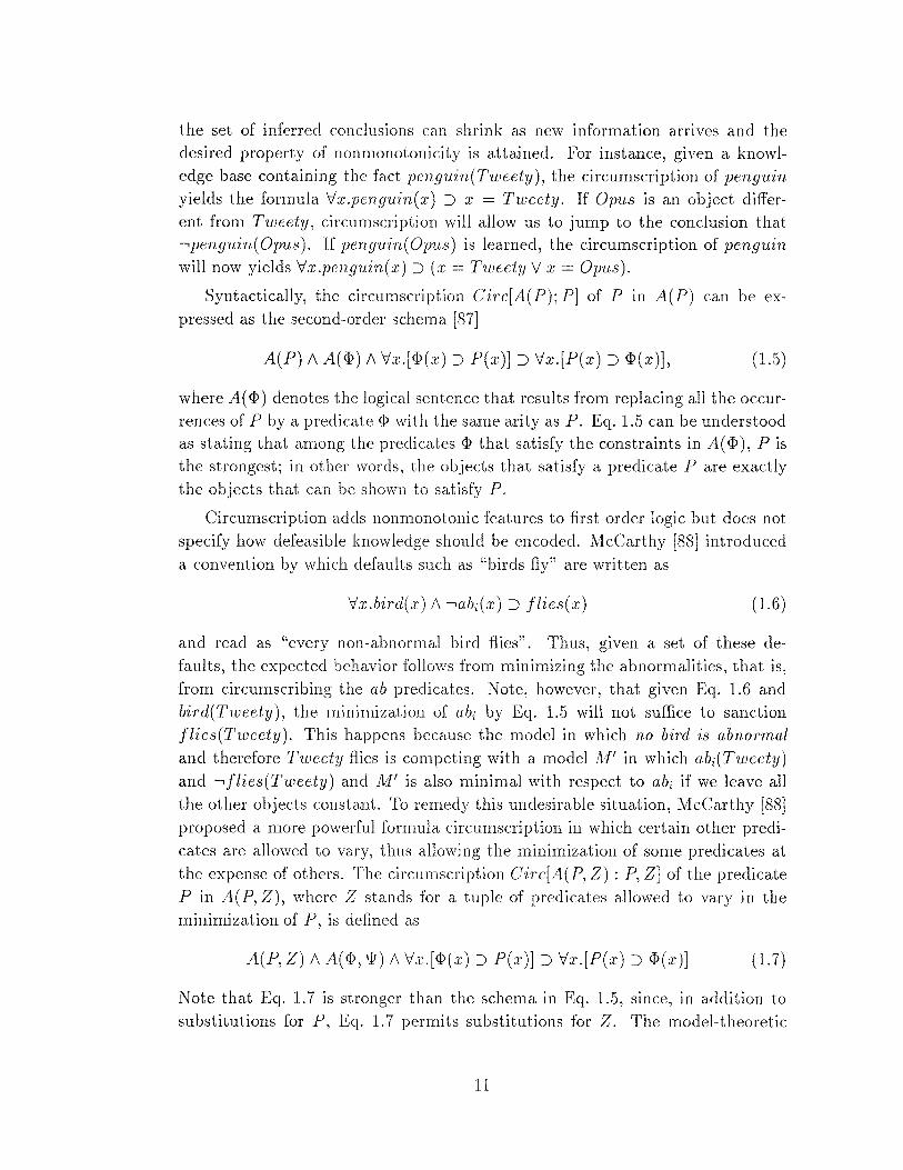
the set of inferred conclusions can shrink as new information arrives and the desired property of nonmonotonicity is attained. For instance, given a. knowl­edge base containing the fact penguin(Tweety ), the circumscription of penguin yields the formula. Vx.penguin(x) :::> x = Tweety. If Opus is an object differ­ent from Tweety, circumscription will allow us to jump to the conclusion that -,penguin( Opus). If penguin( Opus) is learned, the circumscription of penguin will now yields Vx.penguin(x) :::> (x = Tweety V x =Opus).

Syntactically, the circumscription Circ[A(P); P] of P in A(P) can be ex­pressed as the second-order schema [87]

A(P) 1\ A(<])) 1\ Vx.[(J)(x) :::> P(x)] :::> Vx.[P(x) :::> <])(x)], (1.5)

where A(<])) denotes the logical sentence that results from replacing all the occur­rences of P by a predicate <P with the same a.rity asP. Eq. 1.5 can be understood as stating that among the predicates <P that satisfy the constraints in A(<])), P is the strongest; in other words, the objects that satisfy a. predicate P are exactly the objects that can be shown to satisfy P.

Circumscription adds nonmonotonic features to first order logic but does not specify how defeasible knowledge should be encoded. McCarthy [88] introduced a. convention by which defaults such as "birds fly" are written as

Vx.bird(x) 1\ -,abi(x) :::> flies(x) (1.6)

and read as "every non-abnormal bird flies". Thus, given a. set of these de­faults, the expected behavior follows from minimizing the abnormalities, that is, from circumscribing the ab predicates. Note, however, that given Eq. 1.6 and bird(Tweety ), the minimization of abi by Eq. 1.5 will not suffice to sanction flies(Tweety ). This happens because the model in which no bird is abnormal and therefore Tweety flies is competing with a model AI[' in which abi(Tweety) and -,jfies(Tweety) and AI[' is also minimal with respect to abi if we leave all the other objects constant. To remedy this undesirable situation, McCarthy [88] proposed a more powerful formula circumscription in which certain other predi­cates are allowed to vary, thus allowing the minimization of some predicates at the expense of others. The circumscription Circ[ A( P, Z) : P, Z] of the predicate P in A(P, Z), where Z stands for a tuple of predicates allowed to vary in the minimization of P, is defined as

A(P, Z) 1\ A(<]), w) 1\ Vx.[<P(x) :::> P(x)J :::> Vx.[P(x) :::> <])(x)J (1.7)

Note that Eq. 1.7 is stronger than the schema in Eq. 1.5, since, in addition to substitutions for P, Eq. 1.7 permits substitutions for Z. The model-theoretic

11

interpretation of Circ[A(P, Z); P, Z] sanctions as theorems the sentences that hold in all models for A(P, Z) that are minimal in P with respect to Z [78]. A model M of A(P, Z) is minimal in P with respect to Z, if there are no other models M' of A(P, Z) that assign a smaller extension to P and that preserve from M the same domain and the same interpretation of symbols other than P and Z. Note that the expected conclusion, flies(Tweety ), follows in the example above by minimizing the abi predicate while allowing flies to vary since the only minimal models are those in which •abi(Tweety) holds.

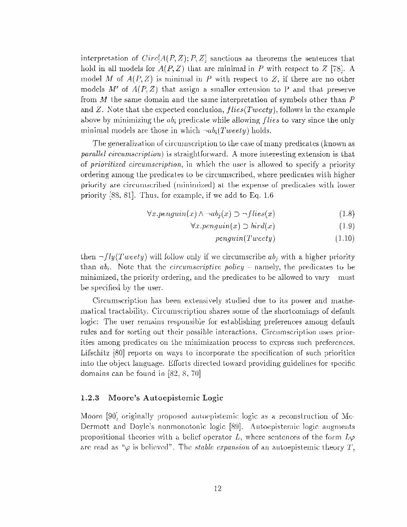
The generalization of circumscription to the case of many predicates (known as parallel circumscription) is straightforward. A more interesting extension is that of prioritized circumscription, in which the user is allowed to specify a priority ordering among the predicates to be circumscribed, where predicates with higher priority are circumscribed (minimized) at the expense of predicates with lower priority [88, 81]. Thus, for example, if we add to Eq. 1.6

Vx.penguin(x) 1\ •abj(x)::) •flies(x)

Vx.penguin(x)::) bird(x)

penguin(Tweety)

(1.8)

(1.9)

(1.10)

then •fly(Tweety) will follow only if we circumscribe abj with a higher priority than abi. Note that the circumscriptive policy - namely, the predicates to be minimized, the priority ordering, and the predicates to be allowed to vary- must be specified by the user.

Circumscription has been extensively studied due to its power and mathe­matical tractability. Circumscription shares some of the shortcomings of default logic: The user remains responsible for establishing preferences among default rules and for sorting out their possible interactions. Circumscription uses prior­ities among predicates on the minimization process to express such preferences. Lifschitz [80] reports on ways to incorporate the specification of such priorities into the object language. Efforts directed toward providing guidelines for specific domains can be found in [82, 8, 70]

1.2.3 Moore's Autoepisternic Logic

Moore [90] originally proposed autoepisternic logic as a reconstruction of Mc­Dermott and Doyle's nonmonotonic logic [89]. Autoepistemic logic augments propositional theories with a belief operator L, where sentences of the form Lcp are read as "cp is believed". The stable expansion of an autoepistemic theory T,

12

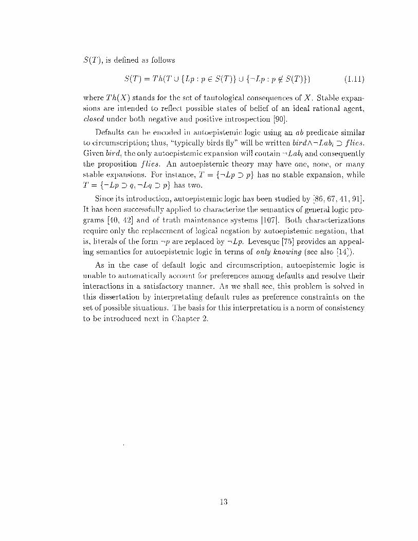
S(T), is defined as follows

S(T) = Th(T U {Lp: p E S(T)} U { --.Lp: p (j. S(T)}) (1.11)

where Th(X) stands for the set of tautological consequences of X. Stable expan­sions are intended to reflect possible states of belief of an ideal rational agent, closed under both negative and positive introspection [90].

Defaults can be encoded in autoepistemic logic using an ab predicate similar to circumscription; thus, "typically birds fly" will be written bird/\ --.Labi =:> flies.

Given bird, the only autoepistemic expansion will contain --.Labi and consequently the proposition flies. An autoepistemic theory may have one, none, or many stable expansions. For instance, T = { --.Lp :::> p} has no stable expansion, while T = { --.Lp :::> q, --.Lq :::> p} has two.

Since its introduction, autoepistemiclogic has been studied by [86, 67, 41, 91]. It has been successfully applied to characterize the semantics of general logic pro­

grams [40, 42] and of truth maintenance systems [107]. Both characterizations require only the replacement of logical negation by autoepistemic negation, that is, literals of the form --.p are replaced by --.Lp. Levesque [75] provides an appeal­ing semantics for autoepistemic logic in terms of only knowing (see also [14]).

As in the case of default logic and circumscription, autoepistemic logic is unable to automatically account for preferences among defaults and resolve their interactions in a satisfactory manner. As we shall see, this problem is solved in this dissertation by interpretating default rules as preference constraints on the

set of possible situations. The basis for this interpretation is a norm of consistency

to be introduced next in Chapter 2.

13

CHAPTER 2

The Consistency of Conditional Knowledge Bases

2.1 Introduction

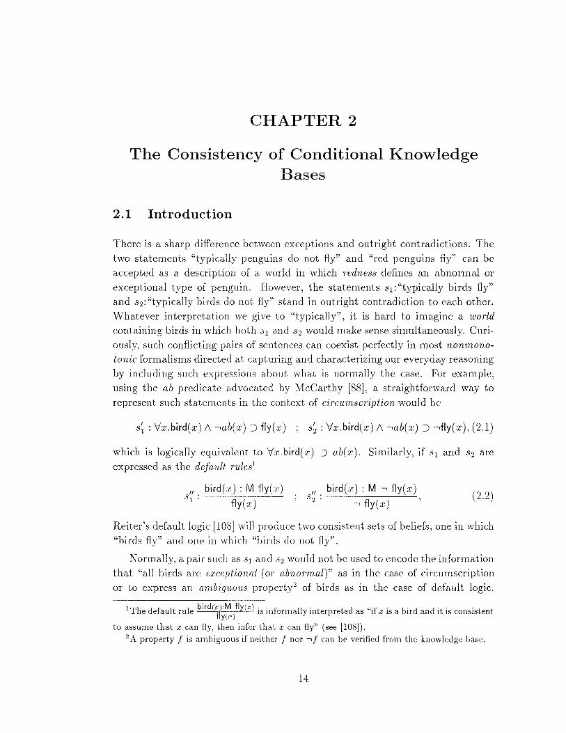
There is a sharp difference between exceptions and outright contradictions. The two statements "typically penguins do not fly" and "red penguins fly" can be accepted as a description of a world in which redness defines an abnormal or exceptional type of penguin. However, the statements s1 : "typically birds fly" and s2 : "typically birds do not fly" stand in outright contradiction to each other. Whatever interpretation we give to "typically", it is hard to imagine a world

containing birds in which both s1 and s 2 would make sense simultaneously. Curi­ously, such conflicting pairs of sentences can coexist perfectly in most nonmono­

tonic formalisms directed at capturing and characterizing our everyday reasoning by including such expressions about what is normally the case. For example, using the ab predicate advocated by McCarthy [88], a straightforward way to represent such statements in the context of circumscription would be

s~: Vx.bird(x) 1\ •ab(x) ::::> fly(x) ; s;: Vx.bird(x) 1\ •ab(x) ::::> •fly(x), (2.1)

which is logically equivalent to Vx.bird(x) ::::> ab(x). Similarly, if s 1 and s2 are expressed as the default 1'ules1

, bird(x): M fly(x) s . --~~--~~~

1 · fly( x)

, bird(x): M • fly(x) ;

32: ·fly(x) '

(2.2)

Reiter's default logic [108] will produce two consistent sets of beliefs, one in which "birds fly" and one in which "birds do not fly".

Normally, a pair such as s 1 and s2 would not be used to encode the information that "all birds are e.rceptional (or abnormal)" as in the case of circumscription or to express an ambiguous property2 of birds as in the case of default logic.

1The default rule bird(ffy~/ly(x) is informally interpreted as "if xis a bird and it is consistent

to assume that x can fly, then infer that x can fly" (see [108]). 2 A property f is ambiguous if neither f nor -.J can be verified from the knowledge base.

14

Rather, this kind of contradictory information is more likely to originate from an unintentional mistake. Remarkably, although humans readily recognize the distinction between exceptions, ambiguities, and contradictions, current work on defeasible knowledge bases presents no comprehensive analysis of such utterances, which could alert the user to the existence of contradictory, possibly unintended statements. As a first step in formulating a framework for representing and

reasoning with if-then rules adrnitting exceptions, this chapter proposes a se­

mantically sound norm for consistency, accompanied by effective procedures for testing inconsistencies and isolating their origins.

It is tempting to assume that pairs such as s 1 and s2 constitute the only source of inconsistency and that once we eliminate such contradictory pairs, the remain­ing knowledge base would be consistent, that is, all conflicts could be rationa.lized as conveying exceptions or ambiguities. Touretzky [122] has shown that this is in­deed the case in the domain of acyclic and purely defeasible inheritance networks.

However, once the language becomes more expressive, allowing hard rules as well as arbitrary formulas in the antecedents and consequents of the rules, the crite­rion for consistency becomes more involved. Consider the knowledge base .6. =

{"all birds fly", "typica.lly penguins are birds", "typically penguins do not fly"}.

This set of rules, although without contradictory pairs, also strikes us as incon­sistent: If all birds fly, there cannot be a nonempty class of objects (penguins) that are "typically birds" and yet "typically do not fly". We cannot accept this knowledge base as merely depicting exceptions; it looks more like a program­ming "bug" or "glitch" than a genuine description of some state of affairs. If we now change the first sentence to read "typically birds fly" (instead of "all birds fly"), consistency is restored; we are willing to accept penguins as exceptiona.l birds. This interpretation vv•ould remain satisfactory even if we made the second

rule strict (to read "all penguins are birds"). Yet, if we add to .6. the sentence

"typically birds are penguins", we again face intuitive inconsistency.

In this chapter we propose a probability-based formalism that captures these

intuitions. We will interpret a defeasible rule "typically, if c.p then '1/J" (written c.p --+ 1/J) as the conditional probability statement P( 1/J lc.p) ~ 1 - s , where s > 0 is an infinitesimal quantity. Intuitively, this amounts to according the consequence 1/J a very high likelihood whenever the antecedent c.p is all that we know. The strict

rule "if ¢ then definitely a-" (written ¢ :::::} J) will be interpreted as an extreme conditional probability statement P( a- I¢) = 1. Our criterion for testing consis­tency translates to determining whether there exists a probability distribution

P that satisfies all these conditional probabilities for every s > 0. Furthermore,

to match our intuition that conditional rules neither refer to empty classes nor are confirmed by merely "falsifying" their antecedents, we also require that P be

15

proper, that is, it does not render any antecedent as totally impossible. These two requirements constitute the essence of our proposal.

In the language of ranked models (see Sees. 3.2, and 4.2, and also [72]), our proposal assumes a. particularly simple form. A defeasible rule <p ------t ·</J imposes the constraints that v) holds in all minimally ranked models of <p and that there will be at least one such model. A strict rule ¢ =?- a imposes the constraint that no possible world satisfies ¢ 1\ •a and that at least one possible world satisfies ¢. Consistency amounts to requiring the existence of a ranking (a mapping of models to integers) that simultaneously satisfies all these constraints. The idea of attach­ing probabilistic semantics to conditional rules goes back to Adams [1, 2], who developed a logic of indicative conditionals based on infinitesimal probabilities. 3

More recently, infinitesimal probabilities were mentioned by McCarthy [88] as a possible interpretation of circumscription and were used by Pearl [95] to develop a graphical consistency test for inheritance networks, extending that of Touret­zky [122]. The proposals in [97, 102, 35, 37] have extended Adams' logic to default schemata, and Lehmann and Magidor [7 4] have shown the equivalence between Adams' logic and a semantics based on ranked models.

Unfortunately, the notion of consistency treated in [2] and [95] was restricted to systems involving purely defeasible rules. This chapter extends Adams' consis­tency results to mixed systems containing both defeasible and strict information, and, as we shall see, the extension is by no means trivial, since a strict rule b =?- J must be given a semantics totally different from its material counterpart b ::::> f. For example, whereas the set of rules {b ::::> J, b ::::> •f} is logically consistent, our semantics must now render the set { b =?- f, b =?- •f} inconsistent. The need to distinguish between b =?- f and b ::::> J, where the former is used to ex­press generic knowledge and the latter as an item of evidence is also advocated in [35, 37, 23, 104] (see Sec. 2.7). The implications of this distinction will become more apparent in Chapter 5, where causality is introduced in the interpretation of the conditional rules.

In addition to extending the consistency criterion to include mixed systems, we also present an effective syntactic procedure for testing this criterion and iden­tifying the set of rules responsible for the inconsistency. Finally, we analyze a notion of entailment based on consistency considerations. Intuitively, a conclu­sion is entailed by a knowledge base if it is guaranteed an arbitrarily high prob­ability whenever the premises are assigned sufficiently high probabilities. This weak notion of entailment was named p-entailment in [2], c:-entailment in [97],

3 A formal treatment of infinitesimal probabilities using nonstandard analysis is given in [74] and also mentioned in [120].

16

and preferential entailment in [69], and it yields (semimonotonically) the most conservative "core" of plausible conclusions that one would wish to draw from a conditional knowledge base [98].

The definition for probabilistic entailment can be partially extended to knowl­edge bases containing strict information using a device suggested by Adams [1] whereby, by definition, conditional rules whose antecedents have probability zero are assigned probability one. Thus, a strict rule such as ¢; =? 0' one could con­ceivably be encoded as the defeasible rule ( ¢; 1\ •0') --+ False. Another proposal was made in the preferential-models analysis of [69]. There, Kraus, Lehmann, and Magidor write (p. 172):

We reserve to ourselves the right to consider universes of reference that are strict subsets of the sets of all models of L. In this way, we shall be able to model strict constraints, such as penguins are bitds, in a simple and natural way, by restricting U to the set of all worlds that satisfy the material implication penguin :=> bitd.

Both of these proposals suffer from two weaknesses. First, they do not capture the common understanding that the opposing pair "all birds fly" and "all birds don't fly" is inconsistent, but instead permit the conclusion that birds do not exist,

together with other strange consequences such as "typically birds have property P" where P stands for any imaginable property. Our semantics reflects the view, also expressed in [23], that one of the previous rules must be invalid and that no admissible model would support both rules. Second, these proposals do not permit us to entail new strict rules in a more meaningful way, according to our commonsense interpretation of conditional sentences, than logical entailment. For

example, •a should not entail a =? b, in the same way that "I am poor" should not entail "if I were rich, it should rain tomorrow". Thus, the special semantics we give to conditional rules, defeasible as well as strict, avoids such paradoxes of material implication [4] and, hence, brings mechanical and plausible reasoning closer together.

This chapter is organized as follows: Section 2.2 introduces notation and some

preliminary definitions. Consistency and entailment are explored in Section 2.3. An effective procedure for testing consistency and entailment is presented in Sec­tion 2.4, while Section 2.5 contains illustrative examples. Section 2.6 deals with

entailment in inconsistent knowledge bases, and the main results are summarized in Section 2.7. All proofs appear in Appendix A.

17

2.2 Notation and Preliminary Definitions

The basic language is a finite set £ of atomic propositions augmented with two propositional constants T and F, which are (informally) regarded as expressing a logical truth and a logical falsehood, respectively. Let Lp be a closed set of propositional well-formed formulas ( wffs) generated as usual from the atomic propositions in £ and the connectives V and •. We define a world w as a truth assignment for the atomic propositions in£. The set of possible worlds is denoted by n, and if there are n atomic propositions in £, the size of n will be 2n. The satisfaction of a wff tp E Lp by a world w is defined as usual and denoted by w f= cp. If w satisfies tp, we say that w is a model for tp.

A d .f '1 1 1 ' L 1 1' ] I 1 d 0 /, rr ' " d eJeaswte T'Ule 1s Lne wrmu a tp --+ 'lp, wnere tp an '+' are wrrs m '-'P an --+ is a new binary connective. Informally, each tp --+ 1/; represents an if-then rule that admits exceptions and each may be read as "if tp then typically 1/;" or "if tp then normally 1/;". Similarly, given ¢, 0' in Lp, the new binary connective =} will be used to form a strict rule ¢ =} 0'. A strict rule ¢ =} 0' is interpreted as "if ¢ then definitely 0'". A formal interpretation of both strict and defeasible rules is given in the definition of consistency (Def. 2.2). Both --+ and =} can occur only as the main connective in a rule. We will use conditional rules or simply rules when referring to a formula. that can be either a defeasible or a strict rule. The antecedent of a rule is the wff to the left of the main connective (single or double arrow) and its conseq11.ent is the wff to the right. If r denotes a conditional rule with antecedent¢ and consequent'!/', then the negation of 1', denoted by rvr, is defined as a conditional with antecedent ¢ and consequent •1/;. The material counterpart of a conditional rule with antecedent tp and consequent 1/; is defined as tp ::::> 1/; (where ::::> denotes material implication), and the material counterpart of a set .6. of conditional rules (denoted by l..) is defined as the conjunction of the material counterparts of the rules in .6..

A default tp --+ 1p is verified by a world w iff w f= tp 1\ '1/J. tp --+ '1/J is falsified by w iff w f= tp 1\ •1/J. Fina.lly, tp--+ 'ljJ is satisfied by w iff w f= tp ::::> 'ljJ. Strict rules are verified, falsified, and satisfied in the same way.

Definition 2.1 (Probability assignment) Let P be a probability function on

the space of possible worlds 0, such that P(w) ~ 0 and I:wEfl P(w) = 1. We define a probability assignment P on a formula cp E £ as

P(tp) = 2:.: P(w). (2.3) wf=cp

Let .6. = DUS be a set of conditional rules such that D = { lpi --+ '1/Ji} ( 1 :::; i :::; IDI) and S = {¢j =? O'j} (1:::; j:::; 151). A probability assignment on a defeasible rule

18

<p ~ ¢ E D is defined as

ifP(cp)>O (2.4)

otherwise

We assign probabilities to the rules in S in exactly the same fashion. P will be considered proper for a conditional rule 1' with antecedent <p if P( <p) > 0, and it will be proper for 6 if it is proper for every conditional in 6. 0

The probability assignment above attaches a conditional probability interpreta­tion to the rules in a given 6. Eq. 2.4 states that the probability of a conditional rule r with antecedent <p and consequent ¢ is equal to the probability of r being verified (i.e., w I= <p 1\ 1/;) divided by the probability of its being either verified or falsified (i.e., w I= <p).

Up to this point the only difference between defeasible and strict rules is syntactic. They are assigned probabilities in the same fashion and are verified and falsified under the same truth assignments. Their differences will become clear in the next section, where we formally introduce the notion of consistency.

2.3 Probabilistic Consistency and Entailment

Throughout the rest of the chapter, 6 denotes a knowledge base of conditional

rules. 6 = D U 5', where D = {'Pi ~ ¢i} (1 :::; i :::; IDI) and S' = { y)j =? O"j}

(1 :::; j :::; lSI).

Definition 2.2 (Probabilistic consistency) We say that 6 = D US' is prob­

abilistically consistent (p-consistent) if for every f > 0, there is a probability assignment P that is proper for 6 such that P(¢[cp) ~ 1- f for all defeasible rules <p ~¢in D and P(O"[q)) = 1 for all strict rules ¢ =? O" in 5'. 0

Intuitively, consistency means that it is possible for all defeasible rules to come as close to certainty as desired, while all strict rules hold with absolute certainty. Another way of formulating consistency is as follows: Consider a constant c > 0 and let P Ll,c: stand for the set of proper probability assignments for 6 such that

if P E PLl,c: then P('~'[<p) ~ 1- f for every <p ~¢ED and P(O"[yi;) = 1 for every y) =? O" E 5'. Consistency insists on P Ll,c: being nonempty for every f > 0.

19

Before developing a syntactical test for consistency (Thm. 2.4), we need to define the concept of toleration.

Definition 2.3 (Toleration) Let r be a rule (either defeasible or strict) with antecedent a and consequent f3. We say that r is tolerated by a set .6. if there exists a world w such that

i=IDI )=lSI w f= a 1\ f3 1\ 'Pi :::> '1/Ji 1\ rPJ :::> O"j • (2.5)

j=l

0

Thus, r is tolerated by a set of conditional rules .6. if there is a world w that verifies x and satisfies every rule in .6. (i.e., no rule in .6. is falsified by w ).

Theorem 2.4 Let .6. = D U 8 be a nonempty set of defeasible and strict 1'ules .

.6. is p-consistent iff every nonempty subset .6.' = D' U 8' of .6. complies with one

of the following:

1. If D' is not empty1 then there must be at least one defeasible rule in D' tolerated by .6.'.

2. If D' is empty (i.e. 1 .6.' = 8') 1 each strict rule in 8' must be tolerated by S'.

The following corollary ensures that, in order to determine p-consistency, it is not necessary to check literally every nonempty subset of .6..

Corollary 2.5 .6. = D U 8 is p-consistent iff we can build an ordered partition

of D = [D1, D2, ... , Dn] whe1'e

1. For alll ~ i ~ n 1 each nde in Di is tolerated by S Uj~7+ 1 Dj.

2. Every rule in S is tolerated by S.

Corollary 2 .. 5 reflects the following considerations (see proof in Appendix A): If .6. is p-consistent, Theorem 2.4 ensures the construction of the ordered partition.

On the other hand, if this partition can be built, the proof of Theorem 2.4 shows that a probability assignment can be constructed to comply with the require­ments of Def. 2.2. Corollary 2.5 yields a simple and effective decision procedure for determining p-consistency and identifying the inconsistent subset in .6. (see

Sec. 2.4).

Before turning to the task of entailing new rules, we need to make explicit a particular form of inconsistency.

20

Definition 2.6 (Substantive inconsistency) Let 6 be a p-consistent set of conditional rules, and let r' be a conditional rule with antecedent ¢. We will say that r' is substantively inconsistent with respect to 6 if 6 U { ¢ -t True} is p-consistent but 6 U { r,t} is p-inconsistent. 0

Nonsubstantive inconsistency occurs whenever the antecedent of a conditional rule is logically incompatible with the strict rules of a consistent set 6. It will become apparent from the theorems to follow that a rule r is nonsubstantively inconsistent with respect to a consistent 6 iff both 6 U { r} and 6 U { rv r} are inconsistent.

The concept of entailment introduced below is based on the same probabilistic interpretation as the one used in the definition of p-consistency. Intuitively, we want p-entailed conclusions to receive arbitrarily high probability in every proper probability distribution in which the defeasible premises have sufficiently high probability and in which the strict premises have probability equal to one.

Definition 2. 7 (p-Entailment) Given a p-consistent set 6 of conditional rules, 6 p-entails cp' -t '1/J' (written 6 l=p cp' -t '1/J') if for all c: > 0 there exists 8 > 0 such that

1. There exists at least one P E P D.,o 4 such that P is proper for cp' -t 'lj/.

2. Every P' E PD.,o satisfies P'('I/J'Icp') 2: 1 - c:.

0

Theorem 2.8 relates the notions of entailment and consistency.

Theorem 2.8 If 6 is p-consistent, 6 p-entails cp' -t '1/J' iff¢' -t •'1/J' is substan­

tively inconsistent with respect to 6.

Def. 2.9 and Theorem 2.10 characterize the conditions under which condi­tional conclusions are guaranteed not only very high likelihood but also absolute certainty. We call this form of entailment strict p-entailment.

4 Recall that given a consistent 6. = DU S, P t::.,o stands for the set of probability assignments proper for 6., such that if P E P t::.,c then P( 7/>I'P) 2: 1- 8 for every 'P ---" 7/> E D and P( ui<P) = 1 for every <;6 :=;. O" E S (see Def. 2.2).

21

Definition 2.9 (Strict p-entailment) Given a p-consistent set ,6. of condi­tional rules, ,6. strictly p-entails ¢' =? 0"

1 (written 6 l=s ¢' =? 0"1

) if for all

c:>O

1. There exists at least one P E P D.,c: such that P is proper for ¢' =? 0"1

•

2. Every P' E PD. ,c: satisfies P' ( O"'j ¢') = 1.

0

Theorem 2.10 If 6 = D U S is p-consistent! 6 strictly p-entails ¢' =? 0"1 iff

S U { i.p1 -+ True} is p-consistent and there exists a subset S' of S such that

i.p1 =? •0"1 is not tolerated by S'.

Examples of strict p-entailment are contraposition, { ¢ =? 1p} l=s '~' =? •¢,5

and chaining { ¢ =? O", O" =? 1p} ¢ =? 1p. Note that strict p-entailment subsumes p-entailment, that is, if a conditional rule is strictly p-entailed, then it is also p­entailed. Also, to test whether a conditional rule is strictly p-entailed, we need to check its status only with respect to the strict set in 6. This confirms the intuition that we cannot deduce "hard" rules from "soft" ones.

Note that the requirements of substantive consistency in Theorem 2.10 and properness for the probability distributions in Definition 2.2 distinguish strict rules from their material counterparts and establish a difference between strict p-entailment and logical entailment. For example, consider the knowledge base

6 = S = { c =? •a}, which is clearly p-consistent. While Li = { c :::::> •a} logically entails c 1\ a :::::> b, 6 does not strictly p-en tail c 1\ a =? b, since the antecedent c 1\ a

is always falsified.

Theorems 2.11 and 2.12 present additional results relating consistency and entailment. They follow immediately from previous theorems and definitions. Versions of these theorems, for the case of knowledge bases containing only de­feasible rules first appeared in [2].

Theorem 2.11 If 6 does not p-entail i.p1 -+ 1j/, and i.p1 -+ 1p1 is substantively

inconsistent with respect to 6, then for all c: > 0 there exists a probability assign­

ment P' E PD.,c: which is proper for 6 and i.p1

-+ 1/J' such that P'(1/J'II.P'):; c:.

Theorem 2.12 If 6 = D US is p-consistent, then it cannot be the case that

1. Both i.p-+ 1/; and i.p-+ •1/; are s1tbstantively inconsistent with respect to 6..

2. Both ¢ =? O" and ¢ =? •O" are substantively inconsistent with respect to S.

5Whenever -qf; is satisfiable.

22

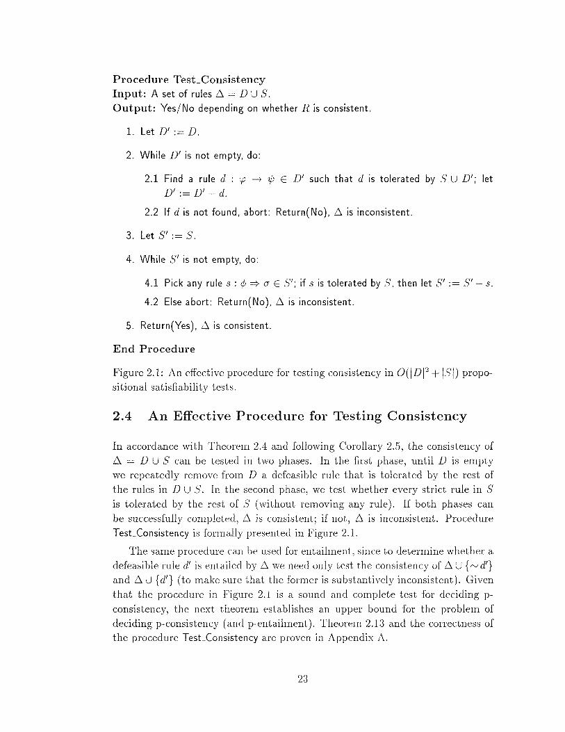
Procedure TesLConsistency Input: A set of rules~ = D US. Output: Yes/No depending on whether R is consistent.

1. Let D' :=D.

2. While D' is not empty, do:

2.1 Find a rule d : cp -t 7/J E D' such that d is tolerated by S U D'; let D' :=D'-d.

2.2 If dis not found, abort: Return( No), ~ is inconsistent.

3. Let S' := S.

4. While S' is not empty, do:

4.1 Pick any rules : cjJ => 0' E S'; if s is tolerated by S, then let S' := S'- s.

4.2 Else abort: Return(No ), ~ is inconsistent.

5. Return(Yes), ~ is consistent.

End Procedure

Figure 2.1: An effective procedure for testing consistency in O(jDj 2 + jSj) propo­sitional satisfiability tests.

2.4 An Effective Procedure for Testing Consistency

In accordance with Theorem 2.4 and following Corollary 2.5, the consistency of ~ = D U S can be tested in two phases. In the first phase, until D is empty we repeatedly remove from D a defeasible rule that is tolerated by the rest of the rules in D U S. In the second phase, we test whether every strict rule in S is tolerated by the rest of S (without removing any rule). If both phases can be successfully completed, ~ is consistent; if not, ~ is inconsistent. Procedure T esLConsistency is formally presented in Figure 2.1.

The same procedure can be used for entailment, since to determine whether a defeasible rule d' is entailed by ~ we need only test the consistency of ~ U { rv d'} and ~ U { d'} (to make sure that the former is substantively inconsistent). Given that the procedure in Figure 2.1 is a sound and complete test for deciding p­consistency, the next theorem establishes an upper bound for the problem of deciding p-consistency (and p-entailment). Theorem 2.13 and the correctness of the procedure TesLConsistency are proven in Appendix A.

23

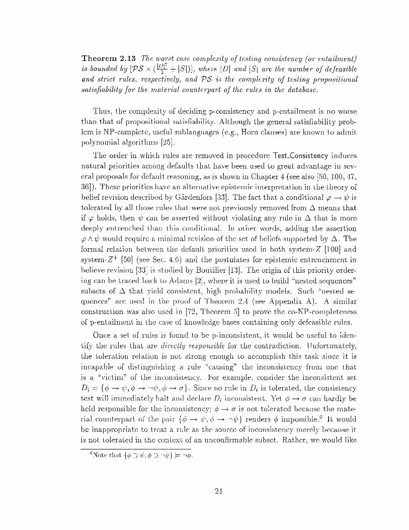
Theorem 2.13 The worst case complexity of testing consistency (or entailment)

is bounded by [PS x ( 1 ~12 + ISI)L where IDI and lSI are the number of defeasible

and strict rules, respectively, and PS is the complexity of testing propositional

satisfiability for the material counterpart of the rules in the database.

Thus, the complexity of deciding p-consistency and p-entailment is no worse than that of propositional satisfiability. Although the general satisfiability prob­lem is NP-complete, useful sub languages (e.g., Horn clauses) are known to admit polynomial algorithms [25].

The order in which rules are removed in procedure T esL(onsistency induces natural priorities among defaults that have been used to great advantage in sev­eral proposals for default reasoning, as is shown in Chapter 4 (see also [50, 100, 47, 36]). These priorities have an alternative epistemic interpretation in the theory of belief revision described by Giirdenfors [33]. The fact that a conditional c.p ----* 1/J is tolerated by all those rules that were not previously removed from .6.. means that if c.p holds, then 1/J can be asserted without violating any rule in .6.. that is more deeply entrenched than this conditional. In other words, adding the assertion c.p 1\ ·1/J would require a minimal revision of the set of beliefs supported by .6... The formal relation between the default priorities used in both system-Z [100] and system-z+ [50] (see Sec. 4.6) and the postulates for epistemic entrenchment in believe revision [33] is studied by Boutilier [13]. The origin of this priority order­ing can be traced back to Adams [2], where it is used to build "nested sequences" subsets of .6.. that yield consistent, high probability models. Such "nested se­quences" are used in the proof of Theorem 2.4 (see Appendix A). A similar construction was also used in [72, Theorem 5] to prove the co-NP-completeness of p-entailment in the case of knowledge bases containing only defeasible rules.

Once a set of rules is found to be p-inconsistent, it would be useful to iden­tify the rules that are directly responsible for the contradiction. Unfortunately, the toleration relation is not strong enough to accomplish this task since it is incapable of distinguishing a rule "causing" the inconsistency from one that is a "victim" of the inconsistency. For example, consider the inconsistent set Di = { ¢> ----* 1/J, ¢> ----* -.'ljJ, ¢> ----* J}. Since no rule in Di is tolerated, the consistency test will immediately halt and declare Di inconsistent. Yet ¢>----* a- can hardly be held responsible for the inconsistency; ¢> ----* a- is not tolerated because the mate­rial counterpart of the pair { ¢> ----* V), c/J ----* -.·ljJ} renders c/J impossible. 6 It would be inappropriate to treat a rule as the source of inconsistency merely because it is not tolerated in the context of an unconfirmable subset. Rather, we would like

6 Note that{¢ :J 1/;,¢ :J •1/J} I= •¢.

24

to proclaim a rule inconsistent if its remova.l would improve the consistency of the database. In other words, a conditional rule r is inconsistent with respect to a set 6 iff there is an inconsistent subset of 6 that becomes consistent after r is removed. Formally,

Definition 2.14 (Inconsistent rule) A rule r is inconsistent with respect to a

set 6 iff there exists a subset 6' of 6 such that 6' U { r} is p-inconsistent but 6' in itself is p-consistent. 0

Deciding whether a given rule is inconsistent is difficult because, unlike the test for set inconsistency, the search for the indicative subset 6' cannot be systematized as in procedure TesLConsistency. All indications are that the search for such a subset will require exponential time. Simple-minded procedures based on remov­

ing one rule at a time and testing for consistency in the remaining set do not yield the desired results. In 6' = {a --+ b, a --+ •b, a --+ c, a =? •c} every rule is incon­sistent, yet it is necessary to remove at least two rules at a time in order to render the remaining set consistent. Likewise, in 6" = {a --+ b, a --+ •b, a --+ c, c =? •b} every rule is inconsistent, yet only the removal of a --+ b renders the remaining

set consistent (or confirmable). Approximate methods for identifying inconsis­tent rules are discussed in Section 2.6 and in the proof of Theorem 2.24 (see Appendix A).

2.5 Examples

The following examples depict some of the rule interactions commonly found in

everyday discourse which motivated the development of nonmonotonic logics and

formalisms for default reasoning. They represent benchmarks in nonmonotonic reasoning and will be used throughout the thesis. As a common denominator, Examples 2.1, 2.2, and 2.3 contain a pair of conflicting rules. Example 2.1 refers to the case of one if-then rule denoting what is generally the case, "if <p then ¢", and another if- then rule representing an exception ( <p and 1) to the first one, "if <p and 1 then •¢". Example 2.2 is similar, except that the antecedents of the

conflicting rules "if <p then '1/," and "if 1 then •'~/'" are related through a third rule, "if 1 then <p", which points out that 1 is a more specific context than a.

Finally, the antecedents in the rules of Example 2.3 are unrelated. Thus, the conflict cannot be resolved and the conclusion remains ambiguous (i.e., neither '1/J nor •'1/' is sanctioned). In all the examples, the rules are modified slightly to highlight the differences between exceptions, contradictions, and ambiguities.

25

Example 2.1 (Dead battery) Consider the following rules:

1. t::::} c ("if I turn the ignition key, definitely the car will start").

2. t 1\ b ~ •c ("if I turn the key and the battery is dead, then normally the car will not start").

This knowledge base is p-inconsistent: Any world w I= t /\ b 1\ --.c (verifying Rule 2, the only defeasible rule) will falsify Rule 1. Intuitively, if the car engine will always start when the ignition key is turned, we cannot accept any faults (e.g., a dead battery). By changing the first rule to be defeasible, we obtain a p-consistent knowledge base 6.c:

1. t ~ c ("if I turn the ignition key, then normally the car will start").

2. t 1\ b ~ •c ("if I turn the key and the battery is dead, then normally the car will not start").

The first rule is tolerated by the second using any world w I= t 1\ •b 1\ c (and once Rule 1 is removed, Rule 2 is trivia.lly tolerated by the remaining empty set). Among the p-entailed conclusions, we have

1. 6.c FP t ~ c ("if I turn the ignition key, then normally the car will start").

2. 6c I=P t 1\ b ~ •c ("if I turn the ignition key and the battery is dead, then normally the car will not start").

3. 6c l=p t ~ -.b ("normally, when I turn the ignition key the battery is not dead").

Example 2.2 (Penguins and birds) Consider the knowledge base presented in the introduction:

1. b ::::} f ("all birds fly").

2. p ~ b ("typically penguins are birds").

3. p ~ •f ("typically penguins don't fly").

Clearly, none of the defeasible rules in the example can be tolerated by the rest. Consider a world w, such that w p 1\ b (testing whether Rule 2 is tolerated). If w I= f Rule 3 will be falsified, while if w I= •f Rule 1 will be falsified. Thus, we conclude that there is no world such that Rule 2 is tolerated. A similar situation

26

arises when we check whether Rule 3 can be tolerated. Thus, this knowledge base is p-inconsistent. Making Rule 1 defeasible yields the so-called "penguin trian­gle", Dp = { b ---+ j, p ---+ b, p ---+ -.J}, which is p-consistent: b ---+ f is tolerated by Rules 2 and 3 through the world w', where w' I= b 1\ J and w' -.p, and, once Rule 1 is removed, the remaining rules tolerate each other. Dp becomes p-inconsistent by adding the rule b ---+ p ("typically birds are penguins"), in con­formity with the graphical criterion of [95]. Note that, by Theorem 2.8, the rule b ---+ -.p ("typically birds are not penguins") is then p-en tailed by Dp. To demon­strate an inconsistency that cannot be detected by such graphical criteria, con­sider adding to Dp the rule p 1\ b ---+ f. Again no rule will be tolerated and the set will be proclaimed p-inconsistent, thus showing (by Thm. 2.8) that p 1\ b ---+ -.J is p-entailed by Dp as expected ("typically penguin-birds don't fly"). Interestingly, all these conclusions remain valid upon changing Rule 2 into a strict conditional p =} b (which is the usual way of representing the penguin triangle), showing that strict class subsumption is not really necessary for facilitating specificity-based preferences in this example.

Example 2.3 (Quakers and Republicans) Consider the following set of rules:

1 ( " . 11 N" . 7 .R bl" ") . n ---+ r typ1ca y 1 1xomtes are . epu 1cans .

2. n---+ q ("typically Nixonites are Quakers").

3. q =} p ("all Quakers are pacifists").

4. r =} -.p ("all Republicans are nonpacifists").

5. p---+ c ("typically pacifists are persecuted").

Rule 5 is tolerated by all others, but the remaining rules are not confirmable, hence inconsistent. The following modification renders the knowledge base con­sistent:

1. n =} ·r ("all Nixonites are Republicans").

2. n =} q ("all Nixonites are Quakers").

3. q---+ p ("typically Quakers are pacifists").

4. r---+ -.p ("typically Republicans are nonpacifists").

7 "Nixonites" is shorthand for people who share aspects of Richard M. Nixon's cultural background.

27

5. p---+ c ("typically pacifists are persecuted").

Indeed, there is a basic conceptual difference between the former case and this one. If all Quakers are pacifists and all Republicans are nonpacifists, our intu­ition immediately reacts against the idea of finding an individual who is both a Quaker and a Republican. The modified knowledge base, on the other hand, allows a Nixonite who is both a Quaker and a Republican to be either pacifist or nonpacifist. Note that both n ---+ p and n ---+ •p are consistent when added to the knowledge base, so neither one is p-entailed and we can assert that the conclusion is ambiguous (i.e., we cannot decide whether a Nixonite is typically a pacifist or not).

Finally, if we make Rules 2 and 4 the only strict rules, we get a knowledge base similar in structure to the example depicted by network r6 in [58]:

1. n---+ r ("typically Nixonites are Republicans").

2. n =? q ("all Nixonites are Quakers").

3. q---+ p ("typically Quakers are pacifists").

4. r =? •p ("all Republicans are nonpacifists").

5. p---+ c ("typically pacifists are persecuted").

Not surprisingly, the criterion of Theorem 2.4 renders this knowledge base consis­tent and n ---+ •p is p-enta.iled in conformity with the intuition expressed in [58].

2.6 Reasoning with p-Inconsistent Knowledge Bases

The theory developed in previous sections presents desirable features from both the semantic and computational standpoints. However, the entailment procedure insists on starting with a p-consistent set of conditional rules. In this section, we relax this requirement and explore two proposals for making entailment insen­sitive to contradictory sta.ternents in unrelated portions of the knowledge base, so that mistakes in the encoding of properties about penguins and birds would not tamper with our ability to reason about politicians (e.g., Quakers and Re­publicans). The first proposal amounts to accepting local p-inconsistencies as

deliberate albeit strange expressions, while the second treats them as program­

ming "bugs".

In Def. 2.1 a. conditional rule <p ---+ 4J was assigned the conditional probability

P(~l<p) if P was pmperfor <p---+ ~(i.e., if P(<p) > 0). In our first proposal for

28

reasoning with p-inconsistent knowledge bases, we will regard improper proba­bility assignments as admissible and define P(7/>lcp) = 1 whenever P(cp) = 0.8

With this approach, any set 6, as long as .6. is logically satisfiable,9 can be rep­

resented by the trivial, high probability distribution in which some antecedents

receive zero probability. Also, strict rules such as ¢ :::} (/ can be represented as

¢1\ •(/---+ False, since we can now use P(¢ 1\ •(/) = 0 to get P((/1¢) = 1. As

before, we say that a rule cp ---+ 1p is implied10 by a (possibly p-in consistent) set

6 if cp ---+ 7/> receives arbitrarily high probability in all probability assignments in

which rules in 6 receive arbitrarily high probability.

Definition 2.15 (prlmplication) Given a set 6 and a rule cp' ---+ 7/>', 6 p1 -

implies cp' ---+ 7/>', written 6 l=p1 cp' ---+ 7/>', if for all £ > 0 there exists a 8 > 0 such

that for all probability assignments P, if P(7/>lcp) 2: 1- 8 for all cp---+ 1/' E 6 and

P((/1¢) = 1 for all¢:::}(/ E 6, then P'(7/>'lcp') 2: 1-£. 0

The only difference between Def. 2.15 and that of p-entailment (Def. 2. 7) is that

none of the probability assignments in the definition above are constrained to be

proper.

Any p-inconsistent 6 will have a nonempty subset violating one of the condi­tions of Theorem 2.4. Given that almost all properties stated in this section will

refer to such sets, we find it convenient to introduce the following definition:

Definition 2.16 (Unconfirmable set) 6 = D US is said to be unconjiTmable if one of the following conditions is true:

0

1. If D is nonempty, then there cannot be a defeasible rule in D that is toler­

ated by 6.

2. If D is empty (i.e., 6 = S), then there must be a strict rule in S that is

not tolerated by 6.

8 Even though P( <p ¢) = 1 if P(<p) = 0 in Def. 2.1, P(<p --+ ¢) was not related to a conditional probability in those cases.

9If Li is not satisfiable this proposal cannot do better than propositional logic, that is, any conditional rule will be trivially entailed.

10We will use the term "implication" instead of "entailment" to stress the fact that the set of premises may constitute a p-inconsistent set. For simplicity, however, we will keep the symbol

29

Note that a set 6.u can be unconfirmable, while both a superset of 6u or one of its subsets can be confirmable. The problem of deciding whether a rule is PI-implied is no worse than that of deciding p-enta.ilment, as shown by the next theorem (proven in [48]).

Theorem 2.17 6 primplies cp -+ 'lj; iff cp -+ •'l/; belongs to an unconfirmable

subset of 6 U { cp -+ •'l/;}.

This unconfirmable subset can be identified using the p-consistency test discussed in Section 2.4 (Fig. 2.1), and it follows that primplication also requires a poly­nomial number of satisfiability tests. Moreover, p-entailment is equivalent to primplication if 6. is p-consistent (see Thm. 2.23). For example, consider the union of Dp = { b -+ f, p -+ b, p -+ •f} of Example 2.2 (encoding the penguin triangle) and the p-inconsistent set Di = { ¢-+ 'l/;, ¢-+ 'V', ¢-+ 0' }. Some of the rules PI-implied by 6, = DP U D, are p 1\ b-+ •f ("typically, penguin-birds don't fly"), b -+ •p ("typically birds are not penguins"), and ¢ -+ 0'. Some of the rules

not primplied by 6i are p 1\ b -+ f and p -+ 'lj;. Thus, despite its p-inconsistency, not all rules are primplied by 6i. However, this example also demonstrates a disturbing feature of PI-implication: Not only ¢ -+ 'lj; and ¢ -+ --,'lj; but also ¢ -+ '0' and ¢ -+ p (where p is any predicate) are p1-implied. Thus, although the natural properties of penguins remain unperturbed by the p-inconsistency of

Di, strange rules such as ¢ -+ p are deduced even though there is no argument to support them (see [58] for similar considerations on inconsistent rules in the context of inheritance networks).

To locate the source of this phenomenon, it is useful to declare a formula to be inconsistent if the formula is False by default.

Definition 2.18 (Inconsistent formula) Given a set 6 and a formula¢, we

say that¢ is an inconsistent formula with respect to 6 iff 6 primplies ¢-+ False. 0

The next theorem relates primplication to Definition. 2.18 and provides an al­

ternative definition of inconsistent formulas in terms of propositiona.l entailment. It is an easy consequence of Theorem 2.17.

Theorem 2.19 Consider a set 6 of conditional n1les and the formulas 0' and 'lj;:

1. 6 FP1 0' -+ 'lj; iff 0' is an inconsistent formula with respect to 6U { 0' -+ •'l/;}.

2. If 0' is an inconsistent fo'rrnula with r·espect to 6, any conditional rule with

0' as antecedent will be p1 -implied by 6.

30

3. A formula (]' is inconsistent with 1'espect to a set ~ iff there exists an un­

confirmable subset ~' of~ such that 6. 1 J= •¢; 11 where (]' is the antecedent

of a 1'ule in ~'.

Theorem 2.19.2 explains why a rule such as ¢; --7 p is primplied by ~;: ¢; is an inconsistent formula with respect to ~i, hence any rule with ¢; as antecedent will be trivially primplied by ~i·

This deficiency of PI-implication is removed in p2 -implication, our second pro­posal for reasoning with p-inconsistent knowledge bases. The intuition behind p2-

implication is that a rule is considered "implied" only if its negation would intro­duce a new p-inconsistency into the knowledge base. Previous p-inconsistencies

are thus considered as programming glitches and are simply ignored.

Definition 2.20 (p2-Implication) Given a set ~' we say that ¢; --7 1p is p2 -

implied by ~' written ~ J=p 2 ¢; --7 1p, iff¢; --7 1/; is not an inconsistent rule with respect to~ (see Def 2.14) but its negation ¢; --7 ·~'is.

0

The requirement that not both ¢; --7 1/; and ¢; --7 •1/; be inconsistent serves two purposes. First, as with p-entailment, it constitutes a safeguard against rules being trivially implied by virtue of their antecedents being false. Second, if both

rules are inconsistent, the contradiction that originates when either is added to ~ must previously have been embedded in ~ and therefore cannot be new. In

our previous example, the rules p 1\ b --7 •f, b --7 •p, and ¢; --7 (]' are p2-implied by ~ii however, contrary to primplication, the rules ¢; --7 1/;, ¢; --7 •1/;, ¢; --7 •(]',

and ¢; --7 p are not. As stated in Theorem 2.23, p2-implication is strictly stronger than PI-implication and is equivalent to p-entailment if the set ~ is p-consistent.

Since the notion of primplication is based on the concept of an inconsis­

tent rule (Def. 2.14 ), there is strong evidence that any procedure for deciding

primplication will be exponential (see Sec. 2.4). To obtain a more efficient de­

cision procedure, we propose to weaken the definition of an inconsistent rule. Instead of testing whether a given rule is responsible for a p-inconsistency, we

will test whether the rule is responsible for creating an inconsistent formula (see

Thm. 2.19).

Definition 2.21 (Weakly inconsistent rule) The rule r is weakly inconsis­

tent with respect to a set ~' iff there exists an unconfirmable subset ~u of

11 Recall that A denotes the conjunction of the material counterparts of the conditional rules

in~-

31

flU {r}, such that 6u f= •¢ but 6~ [#: •¢, where fl~ the antecedent of some rule in flu.

D

This leads naturally to the notion of weak p2-implication.

flu - { r} and ¢ is

Definition 2.22 (wp 2-Implication) Given a set fl, a rule ¢ ---+ '1/J is wp2 -

implied by fl, written 6 l=wp2 ¢ ---+ v), iff 4) ---+ •1/J is weakly inconsistent with respect to fl. D

As in both Pr and p2-implication, the set fli = Dp U Di wp2-implies the rules

p 1\ b ---+ •f, b---+ •p, and ¢ ---+ cr. More importantly, contrary to primplication

(but similar to p2-implication), the undesirable rules ¢ ---+ •cr and ¢ ---+ p are

not wp2-implied by fli and, in general, wp2-implication will not sanction a rule merely because its antecedent is inconsistent. However, unlike p2-implication,

wp2-implication will sanction any rule whose consequence is the negation of an

inconsistent formula (for example, p---+ •¢).

The notion of wp2-implication is situated somewhere between PI-implication

and p2-implication, as the next two theorems indicate. It rests semantically on

both, since it requires the concepts of inconsistent formulas and inconsistent rules.

It also preserves some of the computational advantages of p1-implication.

Theorem 2.23 1. Given a p-consistent set fl, the notions of p-entailment,

p1 -implication, wp2 -irnplication, and p2 -implication are equivalent.

2. Given a p-inconsistent set fl, p2 -implication is strictly stronger than wp2 -

implication, and wp2 -implication is strictly stmnger than PI -implication.

Theorem 2.24 If the set 6 is acyclic and of Hor·n form, wp2 -implication can be

decided in polynomial time.

The need to search for a suitable unconfirmable subset flu (see Def. 2.22) results

in wp2-implication being computationally harder than PI-implication.

2. 7 Discussion

We have formalized a norm of consistency for mixed sets of conditionals, ensur­ing that every group of rules is satisfiable in a non-trivia.l way, one in which the

antecedent and the consequent of at least one rule are both true. We showed that

32

any group of rules not satisfiable this way must contain conflicts that cannot be reconciled by appealing to exceptions or ambiguities and is thus normally con­

sidered contradictory (i.e., unfit to represent world knowledge). Using this norm, we devised an effective procedure to test for inconsistencies and established a

tight relation between entailment and consistency, permitting entailment to be decided by using consistency tests. These tests were shown to require polyno­mial complexity relative to propositional satisfiability. We also discussed ways of drawing conclusions from inconsistent knowledge bases and of uncovering sets of rules directly responsible for such inconsistencies.

One of the key requirements in our definition of consistency is that no con­ditional rule in 6. should have an impossible antecedent and, moreover, that no antecedent should become absolutely impossible as exceptions (to defeasible

rules) become less likely (i.e., as c becomes smaller). This requirement reflects

our understanding that it is fruitless to build knowledge bases for nonexisting classes and counterintuitive to deduce (even defeasibly) conditional rules hav­ing impossible antecedents. Consequently, pairs such as { ¢ ---+ '1/J, ¢ ---+ -.'ljJ} or { ¢ ::::} '1/J, ¢ ::::} -.'ljJ} are labeled inconsistent and treated as unintentional mistakes. The main application of the procedures proposed in this chapter is to a.lert users and knowledge providers of such glitches, in order to prevent undesirable infer­

ences.

This chapter also presents a new formalization for strict conditional rules, within the analysis of probabilistic consistency, that is totally distinct from their material counterparts. The importance of this distinction has been recognized

by several researchers (see [104, 23, 35, 37] and others) and has both theoretical

and practical implications.

In ordinary discourse, conditionals are recognized by universally quantified subsumptions such as "all penguins are birds" or, in the case of ground rules, by the use of the English word "if" (e.g., "if Tweety is a penguin, then she is a bird"). The function of these indicators is to alert the listener that the assertion made is not based on evidence pertaining to the specific individual, but rather on generic background knowledge pertaining to the individual's class (e.g., being a penguin). It is this pointer to the background information that is lost if a conditional rule is encoded as a Boolean expression, and it is this information that is crucial for adequately processing specificity preferences.

Intuitively, background knowledge encodes the general tendency of things to happen (i.e., relations that hold true in all worlds) while evidential knowledge

describes that which actually happened (i.e., relations in our particular world). Thus, conditional rules, both defeasible and indefeasible, play a role similar to

33

that of meta-inference rules: They tell us how to draw conclusions from specific observations about a particular situation or a particular individual, but do not themselves convey such observations. It is for this reason that we chose to use a separate connective, =?, to denote strict conditionals, as is done in [58] in the context of inheritance networks. Strict conditionals, by virtue of pointing to generic background knowledge, are treated as part of the knowledge base, while propositional formulas, including material implications, are used to formulate queries but are excluded from the knowledge base itself. As a result, the rule p =? b is treated as a constraint over the set of admissible probability assignments, while the propositional formula p :) b is treated as specific evidence or a specific observation on which these probability assignments are to be conditioned.

It does indeed make a profound difference whether our knowledge of Tweety's

birdness comes from generic background knovvledge about penguins or from spe­cific observations conducted on Tweety. In natural language, the latter case would normally be phrased by nonconditional rules such as "it is not true that Tweety is both a penguin and a non-bird", which is equivalent to the material

implication penguin(Tweety) :) bird(Tweety ).

The practical aspects of this distinction can best be demonstrated using the penguin example (Ex. 2.2).12 Assume we know that "typically birds fly" and "typically penguins do not fly". If we are told "Tweety is a penguin" and "all penguins are birds", we would like to conclude that Tweety does not fly. By the same token, if we are told "Tweety is a bird" and "all birds are penguins", we would have to conclude that Tweety does fly. However, note that both {p, p :) b}

and { b, b :) p} are logically equivalent to {p, b}, which totally ignores the relation between penguins and birds and should yield identical conclusions regardless of

whether penguins are subclass of birds or the other way around. Thus, when treated as material implications, information about class subsumption is permit­

ted to combine with properties attributed to individuals and therefore this crucial

information gets lost.

This distinction was encoded in [37] by placing strict conditionals together with defaults in a background conte.Ti, separate from the evidential .set which was reserved for observations made on a particular state of affairs. In [72, p. 212] it

is stated that "dealing witl1 hard constraints, in addition to soft ones, involves relativizing to some given set of tautologies". Here, again, strict conditionals and ground formulas would receive different treatment; only the former are permit­ted to influence rankings among worlds. The separate connective =} used in this chapter treatment makes this distinction clear and natural, and the uniform prob-

12Taken from [37].

34

abilistic semantics given to both strict and defeasible rules adequately captures the notion of consistency in systems containing such mixtures.

In Chapter 5, the distinction between :) and :::} is crucial since rules are used to impose a Markovian condition of independence among the atomic propositions in the language, in order to induce causal interpretations, while wffs are used to provide the context of a query.

The notion of p-entailment is known to yield a rather conservative set of con­clusions. For example, let 6.' = {a ----)- b}, and let a, b, c be atomic propositions

in £. It seems reasonable to expect 6.' f=P c 1\ a ---l- b simply because c repre­sents an irrelevant proposition, one with no relation to our knowledge base 6.'. Yet, the rule c 1\ a ---l- b is not p-entailed by 6.. The reason is that the notion of p-entailment requires P( bJa 1\ c) to attain arbitrarily high probability in all those probability distributions in which P( bJa) attains arbitrarily high probabil­

ity. A probability distribution P' where P'(bJa) 2 1 - c; (for every c; > 0) and yet P'(bJa 1\ c) = 0 can be easily built. 13 For this reason, p-entailment is not proposed as a complete characterization of defeasible reasoning. It nevertheless

yields a core of plausible consequences that should be maintained in every system

that reasons defeasibly [97, 98]. Similar problems with irrelevance are shared by all other proposals for nonmonotonic reasoning based on a conditional interpre­

tation of the rules (see, for example, [23, 69, 14, 36]). Extensions of p-entailment presenting solutions to these problems will be explored in Chapters 3, 4, and 5. 14

Nonprobabilistic extensions can be found in [72, 36, 14]. All these formalisms, as well as circumscription [88], default logic [108], and argument-based systems [84, 58], could benefit from a. prelirninary test of consistency such as the one

proposed in this chapte/

13This is not surprising since a --+ b does not say much about the worlds for c or •C.

14Chapters 3 and 4 are independent of each other and can be read in any order.

35

CHAPTER 3

Plausibility 1: A Maximum Entropy Approach

3.1 Introduction

This chapter proposes an approach to nonmonotonic reasoning that combines the principle of infinitesirn.al probabilities (described in Chap. 2) with the principle of maximum entropy in order to extend the inferential power of the probabilistic interpretation of defaults. As pointed out in Sections 1.1 and 1.2, conditional based approaches (such as p-ent ailment) fail to sanction some desirable patterns which are readily sanctioned in common discourse. Their main weakness stems from the failure to properly handle irrelevant information (see Sec. 2.7 and [101, 38]). Recent extensions (Delgrande's proposal [23], rational closure [72], and system-Z [100]) to the conditional based approaches were successful in capturing some aspects of irrelevance, but still suffer from the ills of conservativism, namely, they fail to sanction proper-ty inheritance from classes to exceptional subclasses. For example, given that "birds fly", "birds have beaks", and "penguin-birds don't fly", these extensions fail to conclude that penguin-birds have beaks (despite their being exceptional relative to flying). The maximum entropy formalism described in this chapter is proposed as a well-disciplined approach to extracting implicit (probabilistic based) independencies from fragments of knowledge, so as to overcome those ills. In this respect, the resulting formalism combines the virtues of both the extensional and the conditional based approaches (see Sec. 1.2 for a review of both approaches to default reasoning).

The connection between maximizing entropy and minimizing dependencies has been recognized by several workers [63, 123] and was proposed for default reasoning by Pearl [97, p. 491]. The origin of this connection lies in statistical mechanics, where the entropy approximates the (logarithm of) the number of dis­tinct configurations (assignments of properties to individuals) that comply with certain constraints [12]. For example, if we observe that in a certain population the proportion of tall individuals is p and the proportion of smart individuals is q,

then out of all configurations that comply with these observations, those in which the proportion of smart-and-tall individuals is pq (as dictated by the assumption of independence) constitute the greatest majority; any other proportion of smart-

36

and-tall individuals would permit the realization of fewer configurations, and will correspond to a lower entropy value.

In physics, a configuration stands for the assignment of each particle to a par­ticular cell in position-momentum space, and all distinguishable configurations can be assumed to have equal a priori probabilities. Therefore, the maximum entropy distribution also represents the most likely distribution, that is, the dis­tribution most likely to be found in nature. Indeed, the celebrated distributions of Maxwell-Boltzman and Fermi-Dirac, both maximizing the entropy under the appropriate assumptions, have been observed to hold with remarkable accuracy

and stability.

A similar argument can be invoked to justify the use of maximum entropy in reasoning applications where possible worlds play the role of configurations,

and the constraints are given by observed statistical proportions, for example, "90% of all birds fly" (see Bacchus et al. [7]). Likewise, if we assume that default expressions are qualitative abstractions of probabilities, and that probabilities are degrees of belief that reflect proportions in an agent's experience, then it is also reasonable to assume that our interpretation of defaults, as manifested in discourse conventions, is governed by principles similar to that of maximum entropy. In view of the "most likely" status of the maximum entropy distribution, it is quite possible that discourse conventions have evolved to conform with the

maximum entropy principle for pragmatic reasons; conformity with this principles assures conformity with the highest number of experiences consistent with the available defaults.

The chapter is organized as follows: Section 3.2 recasts the notions behind p-entailment in terms of consequence relations and parameterized probability dis­tributions (PPD).1 This reformulation has the advantages of conceptual simplicity and expressiveness. Each PPD will induce a consequence relation r/J f"'-' IJ on wffs.

A query such as "is IJ plausible in the context of r/;, given the knowledge base 6." will be then evaluated in terms of the set of consequence relations induced by the PPDs admissible with the constraints in 6.. In this manner, each prob­ability model for a given knowledge base can be characterized and cornpared in terms of the plausible conclusions it sanctions. By the same token, comparisons

with other formalisms are also facilitated. It is shown that this reformulation preserves all the properties of p-entailment (see, for example, Thm. 3.10), and that consequence relations are enhanced with a desirable property called Rational

1This special set of distributions present a smoothness property necessary for the computa­tion of the maximum entropy distribution (see Def. 3.1).

37

Monotony. 2 Section 3.3 is concerned with the symbolic machinery necessary to compute the consequence relation associated with the maximum entropy distribu­

tion, and develops such machinery for a class of default rules called minimal-core

sets. Section 3.4 gives examples illustrating the behavior of the consequence relations that results from maximizing entropy. Section 3.5 discusses issues re­lated to non-minimal-core sets, and Section 3.6 summarizes the main results. A step-by-step application of the Lagrange multipliers technique can be found in Appendix B, while Appendix A contains proofs of the main theorems and propositions.

3.2 Parameterized Probability Distributions

The definition below restricts the set of acceptable probability distributions to those that present an analytic property around c = 0. This restriction is con­venient for computing maximum entropy and for introducing the concepts of consequence relations (see Def. 3.4) and rankings (see Def. 3.7). As is demon­strated in Theorems 3.3 and 3.10, this restriction does not affect the notions of p-consistency and p-entailment introduced in Chapter 2.

Definition 3.1 (Parameterized probability distribuion) A parameterized prob­

ability distribution (PPD) is a collection {Pte} of probability measures over the

set n of possible worlds, indexed by a parameter c. { P"} assigns to each possible world w a function of c, P, ( w), such that:

D

1. P"(w) ;:=:: 0 for all c > 0, and

2.::: Pe(w) = 1 for all c > 0. (3.1) wEll

2. For every w, Pc(w) is analytic at c = 0. In other words, PPD's can be

expanded as a Taylor series about zero.

For each formula cp E £, Pe ( cp) is defined as

Pc: ( cp) = 2.::: Pc: ( w), (3.2) wf=<p

2 Ginsberg [44] however, argues against Rational Monotony.

38

and for each '1/J and t.p in £, the conditional probability Pe: ( 'ljJ I'P) is defined as

Pc: ( '1/J I t.p) = { 1

P, ( # cp) P, (cp)

(3.3) otherwise

For simplicity Pc: will be used when referring to the PPD (strictly, {Pe:}) in the remainder of the chapter, wherever the distinction is clear from the context.

Definition 3.2 (Consistency) A given Pc: is admissible with respect to a set D iff for each 'Pi -+ '1/Ji E D,

(3.4)

and Pe:( 'Pi) > 0. D is said to be consistent iff there exists at least one admissible Pe with respect to D.3

0

Theorem 3.3 A set D is consistent iff D is p-consistent.

It follows that procedure T esLConsistency outlined in Figure 2.1 can be used to check consistency as defined in Definition 3.2. The definitions above provide a semantical interpretation for each default rule in D in terms of infinitesimal conditional probabilities, where 1p accrues an arbitrarily high likelihood whenever t.p is all that is known.

As Theorem 3.10 will show, Defs. 3.1 and 3.4 recast the notions of p-entailment in terms of consequence relations. The study of nonmonotonic and default rea­soning in terms of consequence relations was first proposed by Gabbay [32] and further explored in [8.5, 69, 72].

Definition 3.4 (Consequence relations) Every Pc: induces a umque conse­quence relation ~ on formulas, defined as follows:

(3.5)

t.p ~ '1/J is proper 111 Pc: if Pc: ( t.p) > 0 for all c:. The set of proper t.p ~ 'ljJ will be called the proper consequence relation of Pe:. 0

3 Note that we are only dealing with defeasible rules. The generalization to strict rules follows immediately from the concepts introduced in Chapter 2. We just need to augment the conditions for admissibility in Def. 3.2 to include the requirement that for each </Jj :=:} (J"j E S,

P,((J"il<Pi) = 1.

39

Note that a given Pc: is admissible with respect to a set D iff for each i..pi ---+ '1/Ji E D,

i..pi ~ '1/Ji belongs to the proper consequence relation of P6 •

Among the general Tules of inference that a commonsense consequence rela-tion might be expected to obey, the following have been proposed [37, 69, 85]:4

(Logic) If cp f- '1/J, then cp f-v '1/;.

(Cumulativity) If cp f-v '1/J, then cp f-v 1 iff cp 1\ ~1J f-v I·

(Cases) If cp f-v '1/; and1 f-v '1/;, then cp V 1 f-v '1/J.

Kraus et al. [69] introduce a class of preferential models and show that each preferential model satisfies the three laws given above. Moreover, they show that every consequence relation satisfying those laws can be represented as a preferential model. 5 Analogous results were shown in [72] with respect to the

class of ranked preferential models and the set of rules above augmented by the rule of rational monotony:

(3.6)

Theorems 3.5 and 3.6 formalize the relation between a consequence relation in­duced by a PPD and a consequence relation satisfying the rules of inference above. In particular, Theorem :3.6, 'Which follows from the results in [74], constitutes a representation theorem stating that any finite consequence relation that satisfies logic, cumulativity, cases, and rational monotony can be represented by a PPD.6

Theorem 3.5 A PPD consequence relation satisfies the logic, cumulativity, cases,

and rational monotony rules of inference.

Theorem 3.6 Every PPD consequence relation can be Tepresented as a mnked

prefeTential model, and every mnked preferential model with a finite non-empty

state space can be Tepresented as a PPD consequence Telation.

We remark that c:-semantics, as defined in [37, 97] does not comply in general

with the rule of rational monotony. This is because c:-entailment was defined as the intersection of the consequence relations induced by all admissible P6 ,

4 Geffner [37] proposes an additional rule of inference: If t.p -+ 1/; E D, then t.p f-v 1/;. This rule establishes a connection between the defaults in the knowledge base and the consequence relation f'-'. Semantically, this connection is established in this dissertation by interpretating defaults in D as constraints over rankings (see Defs. 3.2 and 3.4).

5They actually use a slightly different set of inference rules which can be shown to be equivalent to those above.

6 Similar results have been obtained independently by Satoh [113].

40

and Fe was not restricted to analytic functions. Thus, the set of admissible Fe's included discontinuous functions, for which the lime-+O in Eq. 3.5 does not exist. By restricting the probability distributions to be analytic at E = 0, we can guarantee that each one of their consequence relations satisfies the rule of rational monotony.

As E approaches zero, the Taylor series expansion of Fe is dominated by the first term whose coefficient is non-zero. Thus, we can define a ranking function on possible worlds using the exponent of this dominant term as follows.

Definition 3. 7 (Ranking) Given a Fe, the ranking function "'P, ( w) is defined as

0

r min{n such that limc--+0 "'P. (w) = l oo

# 0} if Pe ( W) > 0

if Fe(w) = 0 (3.7)

Moreover, according to Eq. 3.2, Fe also induces a ranking on formulas rp:

(3.8)

Proposition 3.8 The follmuing aTe consequences of Defs. 3.1! 3.4! and 3. 7. Given Fe:

1. TheTe is at least one poss1:ble woTld w such that "'P,(w) = 0.

3. We will say that "'P, is admissible with Tespect to D if joT each !.pi ---+ ~)i E D

(3.9)

D is consistent iff there exists at least one admissible mnking "'P, with Tespect to D.

Expressed in terms of ranking functions, the consequence relation induced by a PPD echoes the preferential interpretation for defeasible sentences advocated in [117] according to which ?/J should hold in all minimal (preferred, more normal) models for rp. This can be seen more clearly by writing Eq. 3.9 as"'( rp) < rv( rpA •'1/;) and recalling that, in our case, minimality (preference or normality) is reflected in having the lowest possible ranking (i.e., the highest possible likelihood).

41

The rankings induced by Pe: will prove useful in the maximum entropy com­putation process. Rather than computing the PPD of maximum entropy, P*, we will calculate its corresponding ranking Kp• (denoted K*), from which we can compute the consequence relation associated with P*.

3.3 Plausible Conclusions and Maximum Entropy

Given that ¢; is true, a formula a will be probabilistically entailed by D if

in all Pe: that are admissible with respect to D.

Definition 3.9 (Probabiiistic entailment) Given a consistent D, a formula a is probabilistically entailed by D given ¢;, written ¢; ~ a, iff ¢; 1"'-' a is in the proper consequence relation of all Pe: admissible with D. 0

As is expected there is a close relation between p-ent ailment (Def. 2. 7 and prob­abilistic entailment:

Theorem 3.10 Given a consistent D) ¢; ~ a iff D l=p ¢; -+ a.

It follows that we can use the decision procedure for p-entailment (based on procedure TesLConsistency in Figure 2.1) for deciding probabilistic entailment.7

Probabilistic entailment yields ( semimonotonically) the most conservative "core" of plausible conclusions that one vvould wish to draw from a conditional database if one is committed to avoiding inconsistencies [101]. In particular, it does not permit chaining (from a -+ band b-+ c conclude a 1"'-' c), or contraposition (from a-+ b conclude --.b f-v •a), hence it is too weak to be proposed as a complete char­acterization of defeasible reasoning. As was mentioned in Sections 1.1 and 2. 7, the reason for this conservative behavior lies in our insistence that any conclusion must attain high probability in all probability distributions admissible with D. Thus, given D = {p -+ --,j} ("typically penguins don't fly") and the proposition bl (for "blue"), the conclusion bll\ p ~ --,j ("blue penguins don't fly") will not be sanctioned by probabilistic entailment, since one admissible distribution re­flects a world in which blue penguins do fly. Clearly, if we want the system to

7This notion of entailment is also equivalent to the notion of preferential entailment in [69], even though preferential entailment was motivated by considering desirable features of the consequence relations and not by probabilistic considerations. The relation between these two notions was reported by Kraus eta!. [69].

42

respect the communication convention that, unless stated explicitly, properties are presumed to be irrelevant to each other, we need to restrict the family of

probability distributions relative to which a given query is evaluated. In other words, we should consider only distributions that minimize dependencies, that is, they should contain the dependencies that are absolutely implied by D, but no others.

Since the maximum entropy distribution exhibits this minimal commitment to dependencies, it well be the focal point of the inference procedure. The entropy associated with a distribution Pc: is defined as

H[P":] = - L Pc:(w) log Pc:(w ). (3.10) ll

Given a set D = { yi -+ '1/Ji}, the objective is to compute the PPD among those satisfying the constraints imposed by D that maximizes the entropy; 8 P* denotes

this maximum entropy distribution. The formulas in the consequence relation of P* (denoted by "*"') are then taken as plausible conclusions of D those . In

Eq. 3.5, the default yi -+ 4)£ is interpreted as a constraint on the limit of Pc:( '1/Ji Jcfi) as s approaches zero. To facilitate the maximization of H[Pc:J, these constraints are replaced by equivalent constraints that assign a specific bound to Pc:( '1/Ji Jcfi) for every c > 0. The (unique) maximum entropy distribution for each value of c > 0 is then derived, and finally, its asymptotic solution as s approaches zero is examined.

A PPD P"' satisfies a rule r; : cp; -+ 1pi iff

(3.11)

where Ci is an arbitrary positive coefficient independent of s. Accordingly, the admissibility constraints (Eq. 3.5) are re-written as:

(3.12)

As we shall see, the equations governing the ranking approximation will be inde­pendent of Ci. D~ denotes the set of possible worlds verifying the ruler; and D~ denotes the set of possible worlds falsifying the ruler;, the constraint of Eq. 3.12 can be written

(3.13)

8 The PPD of maximum entropy must also satisfy the normalization constraint Ln P, (w) = 1.

The problem is to max1m1ze Eq. 3.10 subject to the constraints given in Eq. 3.13; one constraint for each rule in D. The most powerful method for solving such optimization problems is the Lagrange multipliers technique [5]. This tech­nique associates a factor a with each constraint (rule) and yields a distribution P* that is expressible as a product of these factors [18]. We will see that, under the infinitesimal approximation (i.e., when c: is close to 0), P*(w) will be pro­portional to the product of the factors (a) associated only with those sentences falsified in w.

At the point of maximum entropy, the status of a constraint such as Eq. 3.13 can be one of two types: active, when the constraint is satisfied as an equality, and passive, when the constraint is satisfied as a strict inequality. Passive con­straints do not affect the point of maximum entropy and can be ignored (see [5]). Unfortunately, the task of identifying the set of active constraints is in itself a hard combinatorial problem. The analysis will begin by assuming a set of active constraints, then we will provide a characterization of knowledge bases called minimal-core sets (Def. 3.11) which are guaranteed to impose only active con­straints, and postpone the discussion of inactive constraints till Section 3.5.

An application of the Lagrange multiplier technique on a set of n active con­straints yields the following expression for each term Pc:(w) (see Appendix B for a step by step derivation) :9

Pc:(v.,') = O:o X II O:r; X II a~~C;e:) (3.14) r;ED;;; r;ED;};

where D;;; denotes the set of rules falsified in w and D"!; denotes the set of rules

verified in w. Motivated by Def. 3.4, we look for an asymptotic solution where each O:r; is proportional to c;Z(r;) for some non-negative integer Z(ri),10 and thus each term of the form a[;C;e:) will tend to one as c: tends to zero. The term a 0

is a normalization constant that will be present in each term of the distribution and thus can be safely ignored. Using P: to denote the unnormalized probability

function, and taking the limit as c: goes to zero, Eq. 3.14 yields:

(3.15) otherwise

9 In Eq. 3.14, o:o = e(.\o-I) and o:,.k = e.\k, where ).0 and >.,, are the actual Lagrange multipliers.

10We take a "bootstrapping" approach: if this assumption yields a solution, then the unique­ness of P* will justify this assumption. Note that the assumption will be satisfied for analytic functions (see Def. 3.1) which eliminate exponential dependencies on f.

Thus, the probability of a given possible world w depends only on the rules that are falsified by that possible world. In other words, any two possible worlds that falsify the same set of rules are (asymptotically) equiprobable. Once the a-factors are computed, we can construct an asymptotic approximation of the desired probability distribution (using the ranking functions of Def. 3. 7) and determine the consequence relation fy of D, according to maximum entropy.

To compute the a-factors we substitute the expression for each P:(w) (Eq. 3.15) in each of the active constraint equations (Eq. 3.13), obtaining:

(3.16)

A few observations are in order. First, Eq. 3.16 constitutes a system of n equations

(one for each active rule) with n unknowns (the a-factors; one for each active rule). Second, since Pc is ana.lytic at c: = 0, we can extract the dominant term in the Taylor expansion of each element in the products of Eq. 3.16 and write ari :::::J aic:Z(ri) where Z(r;) is a non-negative integer. Our task reduces to that of computing the Z's.U Third, we can replace each summation by its dominant term, namely, the term where c: has the minimal exponent. Thus, taking log on

both sides of Eq. 3.16 and writing log ari :::::J log a;+ Z(r;) log c: :::::J Z(ri) log c: yields

(3.17)

where the minimization is understood to range over all possible worlds in n;; and

0~, respectively. Note that the constants C; do not appear in Eq. 3.17; they interact only with the a; coefficients which will be adjusted accordingly to match the constraints in Eq. :3.12.

Since rule T; is falsified in each possible world on the left-hand side of Eq. 3.17,

Z(1·i) will appear in each one of the L:-terms inside the rnin operation and can be isolated:

(3.18)

Although Eq. 3.18 offers a significant simplification over Eq. 3.16, it is still not clear how to compute the values for the Z's in the most general case. We now introduce a class of rule sets D for which a simple greedy strategy (see procedure Z* _order in Figure 3.1) can be used to solve the set of equations above.

11 Each probability term P; ( w) is asymptotically determined once the values of the Z's are computed (see Eq. 3.15).

45

Definition 3.11 (Minimal-Core set) D is a minimal-core (MC) set iff for each rule ri :'Pi ----> 1/Ji E D, its negation 'Pi ----> -.'lj;i is tolerated by D- {<pi ----> 1/Ji}. Equivalently, for each rule Ti there is a possible world that falsifies Ti and no other rule in D. 0

For example, the set Dp of Example 2.2 is MC: w1 I= p !\ b !\ f falsifies p ----> -.f, w2 I= -.p !\ b !\ -.f falsifies b ----> f, and w3 p !\ -.b /\ -.f falsifies p ----> b. On the other hand, changing p ----> -.f top ----> f renders Dp no longer MC. Clearly, deciding whether a set D is MC takes JDJ satisfiability tests. The MC property excludes sets D that contain redundant rules, that is, rules r that are entailed by the P* computed for D - { 7"}. It follows that all default rules in an MC set are active.

Proposition 3.12 If D is an MC set) then; for all defaztlts 7" : <.p ----> ¢ E D; <.p w zp is not in the consequence relation indv,ced by D - { <.p ----> '¢}.

The MC property guarantees that, for each rule Ti E D, there is a possible world Wi in which only that rule is falsified. Thus, since the 1nin operation on the left­hand side of Eq. 3.18 ranges over all possible worlds win which Ti is falsified, the minimum of such possible worlds is Wi, and the constraint equations for an MC set can be further simplified to

(3.19)

Note that since the expression 'L-rjED:;; Z(rj) is equal to the exponent of the most significant c:-term in P*(w), from Definition. 3.7 we have that it is actually equal to "'P•(w), which we denote by""*· Thus, Eq. 3.19 can be rewritten as a pair of coupled equations; the first,

(3.20)

assigns a ranking ""* ( w) to each possible world w once we know the Z*-values on the rules. The second,

Z*(r·i) = min "'*(w) + 1, Ml=.;p;/\,P;

(;3.21)

assigns a value Z* ( Ti) to each rule ri : 'Pi ----> 1/Ji once we know the possible world ranking ""*. We have reduced the computation of the maximum entropy distri­bution to finding a Z* function that is consistent with both Eqs. 3.20 and 3.21. Moreover, given the K:*-ranking, we can decide entailment w by the criterion

(3.22)

46

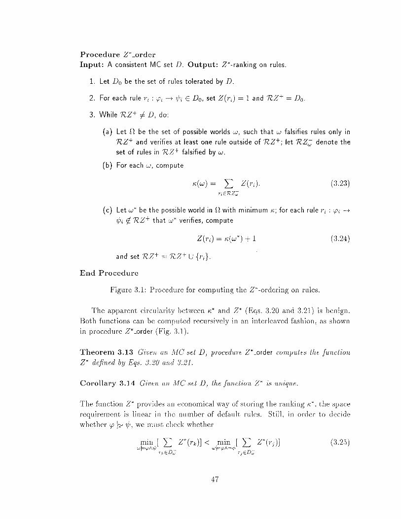
Procedure Z* _order

Input: A consistent MC set D. Output: Z*-ranking on rules.

1. Let D0 be the set of rules tolerated by D.

2. For each rule Ti : yi --+ 1/Ji E Do, set Z(ri) = 1 and nz+ = Do.

3. While nz+ i= D, do:

(a) Let n be the set of possible worlds w, such that w falsifies rules only in

nz+ and verifies at least one rule outside of nz+; let nz:;; denote the

set of rules in nz+ falsified by w.

(b) For each w, compute

A:(w) = L Z(ri). (3.23) r;ERZ:;;

(c) Let w* be the possible world in n with minimum I'C; for each rule 7\ : Cf'i --+

1/Ji tf. nz+ that w* verifies, compute

Z(ri) = fC(w*) + 1 (:3.24)

and set R,Z+ 1(,Z+ U {ri}.

End Procedure

Figure 3.1: Procedure for computing the Z*-ordering on rules.

The apparent circularity between A:* and Z* (Eqs. 3.20 and :3.21) is benign.

Both functions can be computed recursively in an interleaved fashion, as shown

in procedure Z* _order (Fig. 3.1).

Theorem 3.13 Given an !'dC set D, procedure Z* _order computes the function

Z* defined by Eqs. 8.20 and 3.21.

Corollary 3.14 Given an JMC set D, the function Z* is unique.

The function Z* provides an economical way of storing the ranking 11~*, the space

requirement is linear in the number of default rules. Still, in order to decide

whether cp ~ 1/J, we must check whether

(3.25)

47

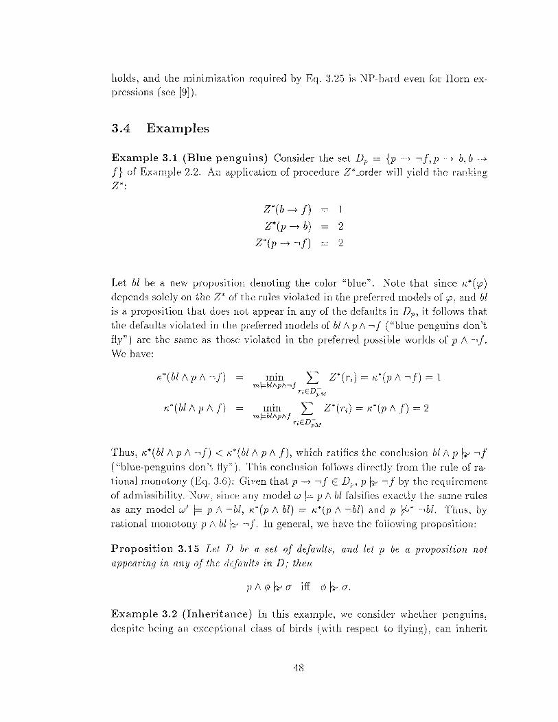
holds, and the minimization required by Eq. 3.25 is NP-hard even for Horn ex­pressions (see [9]).

3.4 Examples

Example 3.1 (Blue penguins) Consider the set Dp {p---+ •f,p---+ b, b---+ f} of Example 2.2. An application of procedure Z* _order will yield the ranking Z*:

Z*(b---+ f) 1

Z*(p---+ b) 2

Z*(p ---+ •f) 2

Let bl be a new proposition denoting the color "blue". Note that since n:*( <p)

depends solely on the Z* of the rules violated in the preferred models of <p, and bl is a proposition that does not appear in any of the defaults in Dp, it follows that the defaults violated in the preferred models of bl 1\ p 1\ •f ("blue penguins don't fly") are the same as those violated in the preferred possible worlds of p 1\ •f. We have:

min L Z*(r;) = n:*(p 1\ •f) = 1 m'p.b/1\p/\-.f _

r;EDpM

n:*(bl 1\p/\ ·f)

n:*(bl 1\ p 1\ f) min L Z*(ri) n:*(p 1\ f) = 2 m'p.b/1\p/\f _

r;EDpM

Thus, n:* ( bl 1\ p 1\ •f) < K~* ( bll\ p 1\ f), which ratifies the conclusion bl 1\ p ~ •f ("blue-penguins don't fly"). This conclusion follows directly from the rule of ra­tional monotony (Eq. ;).6): Given that p---+ •f E Dp, p ~ •f by the requirement of admissibility. Now, since any model w I= p 1\ bl fa.lsifies exactly the same rules as any model w' I= p ;\ ·bl, ~>,*(p 1\ bl) = r~*(p ;\ -.bl) and p bG* •bl. Thus, by rational monotony p 1\ bl ~ •f. In general, we have the following proposition:

Proposition 3.15 Let D be a set of defa'Ults, and let p be a ]J'I'Opositior~, rwt

appearing in any of the defaults in D; then

Example 3.2 (Inheritance) In this example, we consider whether penguins, despite being an exceptional class of birds (with respect to flying), can inherit

48

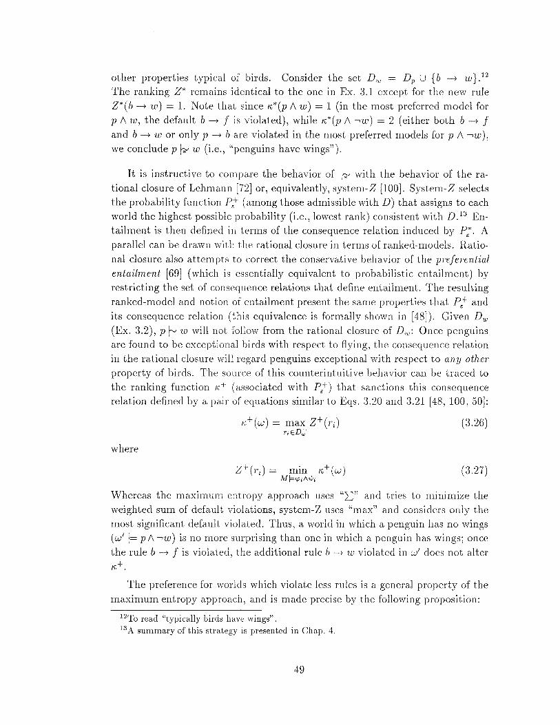
other properties typical of birds. Consider the set Dw = Dp U { b -----? w} .12

The ranking Z* remains identical to the one in Ex. 3.1 except for the new rule Z*(b -----7 w) = 1. Note that since K*(p A w) = 1 (in the most preferred model for pAw, the default b-----? f is violated), while K*(p A •w) = 2 (either both b-----? f and b -----? w or only p -----? b are violated in the most preferred models for p A •w), we conclude p l7 w (i.e., "penguins have wings").

It is instructive to compare the behavior of l7 with the behavior of the ra­tional closure of Lehmann [72] or, equivalently, system-Z [100]. System-Z selects the probability function P,,t (among those admissible with D) that assigns to each world the highest possible probability (i.e., lowest rank) consistent with D. 13 En­tailment is then defined in terms of the consequence relation induced by P;. A parallel can be drawn with the rational closure in terms of ranked-models. Ratio­nal closure also attempts to correct the conservative behavior of the preferential

entailment [69] (which is essentially equivalent to probabilistic entailment) by restricting the set of consequence relations that define entailment. The resulting ranked-model and notion of entailment present the same properties that P,/ and its consequence relation (this equivalence is formally shown in [48]). Given Dw (Ex. 3.2), p ~ w will not follow from the rational closure of Dw: Once penguins are found to be exceptional birds with respect to flying, the consequence relation in the rational closure will regard penguins exceptional with respect to any other

property of birds. The source of this counterintuitive behavior can be traced to the ranking function "'+ (associated with pe+) that sanctions this consequence relation defined by a pair of equations similar to Eqs. 3.20 and 3.21 [48, 100, 50]:

1\~+(w) = max z+(ri) (3.26) r;ED;

where

z+(ri) = min K+(w) M F'Pi 1\ ,P;

(3.27)

Whereas the maxirnurn entropy approach uses "I:" and tries to minimize the weighted sum of default violations, system-Z uses "max" and considers only the most significant default violated. Thus, a world in which a penguin has no wings ( w1 I= p A •w) is no more surprising than one in which a penguin has wings; once the rule b -7 f is violated, the additional rule b -7 w violated in w' does not alter /\,+.

The preference for worlds which violate less rules is a general property of the maximum entropy approach, and is made precise by the following proposition:

12To read "typically birds have wings". 13 A summary of this strategy is presented in Chap. 4.

49

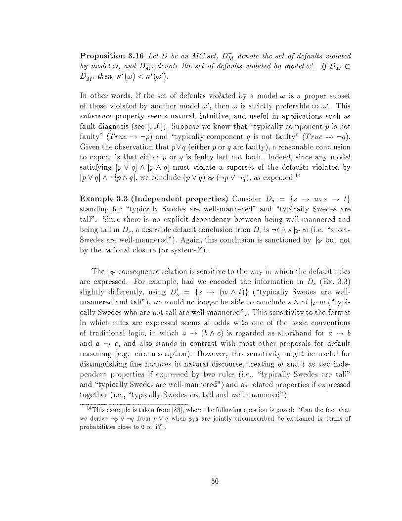
Proposition 3.16 Let D be an MC set} D"M denote the set of defaults violated by model w} and D"M, denote the set of defaults violated by model w'. If D"M C

DM' then} li:*(w) < 1\:*(w').

In other words, if the set of defaults violated by a model w is a proper subset of those violated by another model w', then w is strictly preferable tow'. This coherence property seems natural, intuitive, and useful in applications such as fault diagnosis (see [110]). Suppose we know that "typically component pis not faulty" (T1·ue --+ •p) and "typically component q is not faulty" (Tnte --+ •q). Given the observation that p V q (either p or q are faulty), a reasonable conclusion to expect is that either p or q is faulty but not both. Indeed, since any model satisfying [p V q]/\ [p 1\ q] must violate a superset of the defaults violated by

[p V q]/\ •[p 1\ q], we co11clucle (p V q) ~ (•p V •q), as expectecl. 14

Example 3.3 (Independent properties) Consider Ds = { s --+ w, s --+ t} standing for "typically Swedes are well-mannered" and "typically Swedes are

tall". Since there is no explicit dependency between being well-mannered and

being tall in Ds, a desirable default conclusion from Ds is •t 1\ s ~ w (i.e. "short­Swedes are well-rnannered"). Again, this conclusion is sanctioned by ~ but not by the rational closure (or system-Z).

The ~ consequence relation is sensitive to the way in which the default rules are expressed. For example, had we encoded the information in Ds (Ex. 3.3) slightly differently, using D~ = { s --+ ( w 1\ t)} ("typically Swedes are well­mannered and tall"), we would no longer be able to conclude s 1\ •t ~ w ( "typi­cally Swedes who are not ta.ll are well-mannered"). This sensitivity to the format

in which rules are expressed seems at odds with one of the basic conventions of traditional logic, in which a --+ (b 1\ c) is regarded as shorthand for a --+ b and a --+ c, and also stands in contrast with most other proposals for default reasoning (e.g. circumscription). However, this sensitivity might be useful for distinguishing fine nuances in natural discourse, treating w and t a.s two inde­pendent properties if expressed by two rules (i.e., "typically Swedes are tall" and "typically Swedes are well-mannered") and as related properties if expressed together (i.e., "typically Swedes are tall and well-mannered").

14This example is taken from [8:3], where the following question is posed: "Can the fact that we derive •p V •q from p V q when p, q are jointly circumscribed be explained in terms of probabilities close to 0 or P".

50

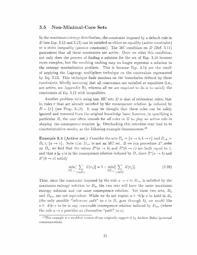
3.5 Non-Minimal-Core Sets

In the maximum entropy distribution, the constraint imposed by a default rule in D (see Eqs. 3.12 and 3.13) can be satisfied as either an equality (active constraint) or a strict inequality (passive constraint). The M C con eli tion on D (De f. 3.11) guarantees that all these constraints are active. Once we relax this condition, not only does the process of finding a solution for the set of Eqs. 3.18 become more complex, but the resulting ranking may no longer represent a solution to the entropy maximization problem. This is because Eqs. 3.18 are the result

of applying the Lagrange multipliers technique on the constraints represented by Eq. 3.12. This technique finds maxima on the boundaries defined by these constraints, blindly assuming that all constraints are satisfied as equalities (i.e., are active, see Appendix B), whereas all we are required to do is to satisfy the constraints of Eq. 3.12 with inequalities.

Another problem with using non MC sets D is that of redundant rules, that is, rules r that are alrea.dy satisfied by the consequence relation ~ induced by D - { r} (see Prop. 3.12). It may be thought that these rules can be safely ignored and removed frorn the original knowledge base; however, in specifying a particular D, the user often intends for all rules in D to play an active role in

shaping the consequence relation ~- Overlooking this intention may lead to to counterintuitive results, as the following example demonstrates. 15

Example 3.4 (Active set.) Consider the sets Da = {a -r b, b -r c} and Da+ =

Da U {a -r c }. Note that Da+ is not an MC set. If we run procedure Z* _order on Da, we find that the values Z*(a -r b) and Z*(b -r c) are both equal to 1, and that a ~ cis in the consequence relation induced by Da since Z*( a -r b) and Z* ( b -r c) satisfy

(3.28)

Thus, since the constraint irnposed by the rule a -r c in Da+ is satisfied by the maximum entropy solution to Da, the two sets will have the same maximum

entropy solution and the same consequence relation. Yet these two sets, Da and Da+, are not equivalent: \,Yhile we do not expect a 1\ -.b ~ c to hold in Da (the only possible "inference path" to c in Da goes through b), we would like a 1\ -.b f'v c to be in any reasonable consequence relation induced by Da+ (where the rule a-rc provides an alternative "path" to c).

15This example is a modified version of one originally suggested by Andrew Baker (personal communication).

51

The problem rests with using the equality Pc(cia) = 1- C x c: as a constraint to the maximization process,16 where in fact the constraint intended by the user is stronger, requiring a faster convergence of Pe:* (cia) towards 1. The use of the Lagrange multipliers technique requires a commitment to a particular rate of

convergence for each rule. Had we started with the insight that limc---+O P( cia) = 1 should be represented by P(cia) = 1 - C x c2 instead, the problem could have

been solved using Eq. :3.18; all constraints in Da+ will be active, yielding

(3.29)

and the consequence relation ~ induced by Da+ will satisfy a 1\ •b ~ c.

In general we could write Eq. 3.18 in terms of slack var-iables Tt; for each constraint,

(3.30)

and seek the correct va.lues of ni that would render every rule active. Computa­tionally, however, guessing the ni's is not easier than guessing the set of active constraints.

We see that the advantages of MC sets are twofold: They guarantee conver­gence of procedure Z* _order to a solution of Eq. 3.18, and this solution represents a solution to the entropy maximization problem. Unfortunately, to ensure these guarantees the expressiveness of the knowledge bases must be limited to MC,

which may prevent us front specifying certain rule sets in the most natural way. It turns out that the class of knowledge bases where these guarantees hold is in fact wider than MC, since Eqs. 3.16 and 3.17 are valid as long as all rules are active. Consider the set Dp of Example 2.2,17 augmented with the rule p -t a

("typically penguins live in the Antarctic"). This set is not M C since any nwdel falsifying p -t a must fa.lsify at least one other default in Dp. Nevertheless, all

rules in DP U {p -t a} are active. Notice that p -t a is insensitive to the Z-values associated with each of the rules in Dp, and vice versa. In other words, any change on the value of the Z associated with a rule in Dp will not affect the Z associated with p -t a. 18 '1'hus, we can compute the Z-values for Dp and p -t a

16 Note that P6 (cia) 2: 1 - C x c: is equivalent to C' x c: x Pe ( c !\a) 2: P6 ( --.c !\a) for expressing lim, ..... 0 P(cia) = 1 as a constraint for the maximization process.

17Recall that Dp {p , p-+ b, b-+ !}. 18The instance of Eq. 3.18 for p a shows that the min-terms on both sides are identical

and therefore can be canceled.

52

separately using two independent applications of procedure Z* _order, one on Dp and the other on p -+ a, and then combine the resulting Z's. We see that cer­tain topological features of D permit its decomposition into a set of components belonging to MC, hence every rule will be active. The full characterization of databases in which all rules are active remains an open problem.

3.6 Discussion

Maximum entropy can be viewed as an extension of both p-entailment and the ra­tional closure. Like p-entailment, it is based on infinitesimal probability analysis; and like rational closure, it is based on a unique ranking of possible worlds sub­ject to constraints. In the rational closure, however, possible worlds are given the lowest rank that is consistently possible, and hence the rank of a model is equal to the rank of the most cTucial rule violated by that model. 19 In contrast, maxi­mum entropy ranks models according to the weighted sum of rule violations, and

it is this difference that enables maximum entropy to sanction inheritance across

exceptional subclasses, concluding that "penguins have wings" in Example 3.2 and that "short Swedes are well-mannered" in Example 3.3.

The ranking of rules in maximum entropy is reminiscent of abnormality pref­erences in prioritized circumscription [88], with the difference that the priorities assigned by maximum entropy are extracted autmTlatically from the knowledge base and do not need the intervention of the user. This property is shared by Geffner's [36] conditional entailment, which also combines the virtues of the exten­sional and the conditiona.l approaches. Conditional entailment maintains partial

orders among rule priorities and among models, and it produces more acceptable

inferences than maximum entropy in certain cases (see [36]), at the expense of a greater computational complexity and the loss of the underlying probabilistic semantics.

A weakness of the maximum entropy approach is that it stands at odds with the principle of causation. 20 If we first compute the maximum entropy distri­bution P* CX1 , . .. , Xn) on a. set of variables X 1 , ... , Xn and then consider one of their consequences Y, we may find that the maximum entropy distribution

P*(X1 , •.. ,Xn,Y) constrained by the conditional probability P(YIX1, ... ,Xn) changes the probabilities of the X variables. For example, specifying the biases

19This ranking is called Z-rank in [100]. 20This weakness, shared by many proposals for nonmonotonic reasoning [57], has required

the introduction of special causal operators (116, 36]. Chapter 5 proposes a different approach to causality based on probabilistic considerations of independence.

53

of two coins yields a rnaximum entropy distribution in which the two coins are mutually independent. However, further specifying the probability with which an observer would respond to each of the four outcomes of these coins might yield a maximum entropy distribution in which the two coins are no longer inde­

pendent of each other (see [97, pp. 463, 519], and [60]). 21 This stands contrary to our conception of causality in which the forecasting of future events does not

alter beliefs about past events. This behavior prevents the maximum entropy

approach from properly handling tasks such as the Yale shooting problem [57], where rules of causal character are given priority over other rules. Such priorities can be introduced in the A:-ranking system using a device called stratification (see Chap. 5), which forces A: to obey the so-called Markov condition: Knowing the present renders the future independent of the past. The role of maximum entropy in stratified rankings could then be to define preferred rankings under incomplete specification of causal influences: Out of all admissible rankings that conform to the stratification condition, choose those with the maximum entropy.

The maximum entropy formalism can be extended to admit defaults with variable strengths; each default in D can be annotated with a parameter 8i, that

indicates the firmness with which the default is believed. 22 Probabilistically, 8i represents the slowest rate at which P(~il<?i) should be allowed to approach one as E approaches zero. The constraints to the maximization process can be modified accordingly; thus, Eq. 3.12 will now read

C\ X

and, given an MC set D, Eqs. 3.20 and 3.21 translate to

t-:* ( w)

Z*( r;)

L Z*(r;)

min A:*(w) + 1 + 8i WF'Pi /\1/;;

(3.31)

(3.32)

(3.33)

where the Z*-order for each rule can be computed using procedure Z* _order.

This feature is very useful in domains such as circuit diagnosis where the analyst may feel strongly that failures are more likely to occur in one group of

devices (e.g., multipiers) than in another (e.g., adders). For example, suppose that in addition to the information "typically component p is not faulty" and "typically component q is not faulty", we also know that component p is much

21 Pearl attributes the discovery of this phenomenon to Norm Dalkey [97]. 22 An extension to system-Z [100] along these lines can be found in Chapter 4 (see also

[50, 53]).

54

more likely to fail than component q. We can encode this information by spec­ifying D = {True •p, True ~ --,q} where 81 < 82 • Thus, given that p V q

(either p or q are faulty) holds, we conclude that p is the faulty component with the failure ( (p V q) ~ (p 1\ •q)). If entailment is defined as the intersection of the ~ consequence rela.tions induced by all sets of values 8i, then the resulting entailment relation will be supported by partial orders among rules and models, a.s in Geffner's [36] conditional entailment.

Chapter 4 studies such an extension to Pearl's system-Z [100], in which each 'P -+ '1/J is annotated with a positive integer 8 denoting the degree of strength or firmness of the rule.

55

CHAPTER 4

Plausibility II: System-z+

4.1 Rankings as an Order-of-Magnitude Abstraction of Probabilities

Regardless of how we choose to interpret default statements, it is generally ac­knowledged that some defaults are stated with greater firmness than others. For example, the action-response defaults of the type "if Fred is shot with a loaded gun, Fred is dead" are issued with a greater conviction than persistence defaults of the type "if Fred is a.live at timet, he is alive at t + 1". Moreover, the degree of conviction in this last statement should clearly depend on whether t is mea­

sured in years or seconds. In diagnosis applications, likewise, the analyst may feel strongly that failures are more likely to occur in one type of device (e.g., multipliers) than in another (e.g., adders). A language must be devised for ex­pressing this valuable knowledge. Numerical probabilities or degrees of certainty

have been suggested for this purpose, but if the full precision provided by numer­ical calculi is not necessary, an intermediate qualitative language might be more

suitable.

This chapter proposes such a language in terms of the ranking functions in­troduced in Chapter 3 (Def. 3.7). This method of approximation gives rise to a

semi qualitative calculus of uncertainty: Degrees of (dis) belief are ranked by non­negative integers (corresponding perhaps to linguistic quantifiers such as "believ­

able", "unlikely", "very rare", etc); retraction and restoration of beliefs conforms to Bayesian conditionalization.

One way of motivating ranking systems is to consider a probability distribu­tion P defined over a set n of possible worlds and to imagine that an agent wishes to retain an order-of-magnitute approximate of P. The traditional engineering method of approximating P would be to express each numerical parameter (spec­ifying P) in a base b representation, where b depends on the precision needed, and then omit all but the most significant figure from each expression. 1 All arithrnetic

1Thus, given a number n and a basis b, its approximate would be the polynomial expression

( )0 ( 1 •) ao* b +a1* b) +a2*(b)~+ ....

56

operations would then be performed on these approximate, single digit quanti­ties, in lieu of the original parameters. The abstraction we advocate goes one step further. Instead of retaining the numerical value of the most significant fig­ure, we retain only its position. The mechanics of this exercise is equivalent to, and can best be described by, a limit process where quantities are reqresented as polynomials in an infinitesimal number E. These polynomials are added and multiplied precisely, but at the end we ca.lculate the limit of the final results as E

goes to zero.

Imagine that the probability P(w) is a polynomial function of some infinites­

imal parameter E, arbitrarily close to, yet larger than zero; for example, P(w) = 1-c1c: or c: 2 -c2 c:4

.2 Accordingly, the probabilities assigned to any subset of n rep­

resented by a logical formula. cp, as well as all conditional proqabilities P(f[cp ), will be rational functions of c. VIe define the ranking function rv('f [cp) as the

power of the most significant E-term in the expansion of P(?,b[cp). In other words, A:(7j;[cp) = n iff P(1p[cp) has the same order of magnitude as En (see Def. 3.7).3

Thus, instead of measuring probabilities on a scale from zero to one, we can imagine projecting probability measures onto a quantized logarithmic scale and then treating beliefs that map onto two different quanta as being of different orders of magnitude.

The following properties of ranking functions (left-hand side below) reflect, on a logarithmic scale, the usual properties of probability functions (right-hand

side), with min replacing addition, and addition replacing multiplication:

minA:(w) wi='P

!i:(cp) = 0 or 11:(•cp) = 0

!i:( <P 1\ cp) = /\tv) I'P) + !i:( cp)

P(cp) = L P(w) ( 4.1) wi='P

P(c.p) + P(•cp) = 1

P(<f; 1\ cp) = P(?,b[cp)P(cp)

Parameterizing a probability measure byE and extracting the lowest exponent of E as the measure of ( clis)belief was proposed in [98] as a model of the process by which people abstract qualitative beliefs from numerical probabilities and accept them as tentative truths. For example, we can make the correspondence between linguistic quantifiers and depicted in Table 4.1 These approximations yield

2 Probability functions parameterized on f were called PPD's in Chapter 3. They are formally introduced in Definition :3.1, where the f-functions were restricted to be analytical in f = 0. The probability functions described above can also be viewed as the Taylor approximation of these PPD's.

3 Spohn [120) was the first to study such ranking functions, which he named (non­probabilistic) ordinal condition function (OCF). His main motivation was to account for the dynamics of plain beliefs.

57

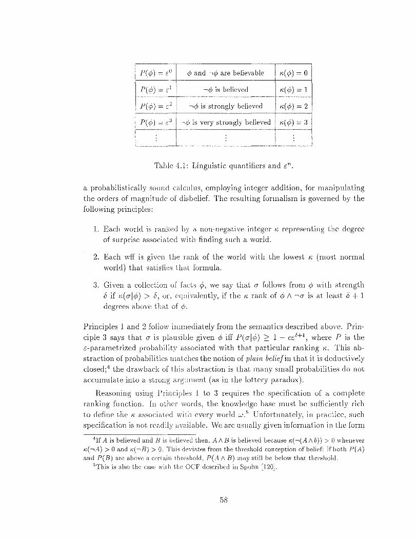
P(¢) = s0 ¢ and •¢ are believable "'( ¢) = 0

P(¢)=E 1 •¢ is believed "'(¢) = 1

P(¢) = s 2 -,¢ is strongly believed "'( ¢) = 2

P(¢) = s3 is very strongly believed "'( ¢) = 3

Table 4.1: Linguistic quantifiers and c;n.

a probabilistically sound calculus, employing integer addition, for manipulating the orders of magnitude of disbelief. The resulting formalism is governed by the following principles:

1. Each world is ranked by a non-negative integer "' representing the degree of surprise associated with finding such a world.

2. Each wff is given the rank of the world with the lowest "' (rnost normal world) that satisfies that formula.

3. Given a collection of facts </J, we say that G follows from <P with strength

8 if K,(GI</J) > 8, or, equivalently, if the"' rank of <P 1\ •G is at least 8 + 1 degrees above that of </J.

Principles 1 and 2 follow immediately from the semantics described above. Prin­ciple 3 says that G is plausible given <P iff P( G I <P) 2 1 - cc; 8+1, where P is the c;-parametrized probability associated with that particular ranking "'· This ab­straction of probabilities matches the notion of plain belief in that it is deductively closed;4 the drawback of this abstraction is that many small probabilities do not accumulate into a strong argument (as in the lottery paradox).

Reasoning using Principles 1 to 3 requires the specification of a complete ranking function. In other words, the knowledge base must be sufficiently rich to define the "' associated with every world w . .s Unfortunately, in practice, such specification is not readily available. We are usually given information in the form

4If A is believed and B is believed then, AI\B is believed because A:(•(A/\b)) > 0 whenever A:( -,A) > 0 and A:( -,B) > 0. This deviates from the threshold conception of belief: if both P(A) and P(B) are above a certain threshold, P(A 1\ B) may still be below that threshold.

5This is also the case with the OCF described in Spohn [120].

58

of statements such as "birds normally fly" which we interpret as P(f[b) ~ 1 - c;

or, equivalently, !i:( -.j[b) > 0, and no information whatsoever about the flying habits of red birds or non-birds. In this case, we still would like to conclude "red birds normally fly", even though the information given merely constraints li: to

satisfy !i:(f 1\ b) < !i:(-.f 1\ b) ("it is less surprising to find a flying bird than a non-flying one"), and is not sufficient for defining a complete ranking function. Drawing plausible conclusions from such fragmentary pieces of information, re­quires additional inferential machinery to accomplish two functions: It should enrich the specification of the ranking function with the needed information, and it should operate directly on the specification sentences in the knowledge base, rather than on the rankings of worlds (which are too numerous to list). Such ma­

chinery is provided by a formalism called system-z+' described in this chapter' which accepts knowledge in the form of graded if-then rules and computes the plausibility of any given query by syntactic manipulation of these rules.

To accomplish these functions, system-z+ incorporates two principles in ad­dition to those given a.bove:

4. Each input rule "if cp then 1/J (with strength 8)", written cp ~ 1/J, is in­terpreted as a constraint on the ranking !i:, forcing every world in cp 1\ -.'ljJ to rank at least 8 + I degrees above the most normal world in cp, that is,

K(1/J[cp)>8.

5. Out of all rankings satisfying the constraints above, we adopt the rank­ing K+ that assigns each world the lowest possible (most normal) rank. Remarkably, this ranking will turn out to be unique.

Principle 4 is a straightforward generalization of the probabilistic reading of the rules, P( 1/J [cp) ~ 1 - cc;S+1

. The parameter 8 is an optional feature for the rule

encoder that augments tbe expressiveness of the knowledge base by assigning strength to the rules. If 8 is unspecified, it is assumed to be equal to zero, and rules are interpreted as P(?/'[cp) ~ 1 - cc:. A knowledge base with all 8 = 0 will be called a flat knowledge base. Remarkably, the addition of the 8's does

not increase the complltational complexity of query-answering and consistency testing. 6 Moreover, we shall see that even a flat knowledge base induces a natural priority on rules in order to respect specificity considerations (see Thm. 4.14).

Principle 5 reflects the assumption of maximal ignorance; unless compelled otherwise, assume every situation to be as normal as possible (or equivalently, no situation is more surprising than necessary). In contrast, the approach based on

6 Both will require a polynornial number of propositional satisfiability tests.

59

maximum entropy (Chap. 3 selects the ranking "'* that minimizes dependencies among propositions, to reflect only those implied by the rules in the knowledge base. As will be seen, the advantage of system-z+ is that the algorithm necessary for computing plausible conclusions is more efficient than the one for maximum entropy (Sec. 3.3). As in the case of maximum entropy, a key step in the procedure is the computation of a priority ordering z+ on the rules in the knowledge base. 7

Section 4.3 (after some preliminary definitions in Sec. 4.2), introduces a procedure that computes z+ in a polynomial number of propositional satisfiability tests and hence is tractable in applications permitting restricted languages, such as Horn expressions, network theories, or acyclic databases. Once the ordering z+ is known, the degree to which a given query is denied or confirmed can be computed in O(logl61) satisfiability tests (where 161 is the number of rules in the knowledge base 6). On the other hand, as shown in Section 4.7 and partially discussed in Sections 3A and 3.6, this computational advantage of system-z+ over maximum entropy, results in weakening the set of conclusions ratified by the system.

In Section 4.5, systern-z+ is equipped with the capability to reason with soft

evidence or imprecise observations. Such a capability is important when we wish

to assess the plausibility of CJ (using Prin. ;3 above) but the context ¢; is not given with absolute certainty; all that can be ascertained is "¢ is supported to a degree n". We propose two different strategies for computing a new ranking "'' from an initial one 1~, given soft evidential report supporting a wff ¢. The first strategy, named .J-condilionalization, is based on Jeffrey's rule of condition­ing [99]. It interprets the report as specifying that "all things considered", the

new degree of disbelief for --,¢; should be "'' ( --,q;) = n. The second strategy, named L-conditionalization, is based on the virtual evidence proposal described in [97, Chap. 2]. It interprets the report as specifying the desired shift in the degree of

belief in ¢, as warranted by that report alone and "nothing else considered". We

show that both J and L-collditionalization have roughly the same complexity as ordinary conditionalization. Section 4.6 relates and compares system-z+ to the

theory of belief revision in [:3]. Finally, Section 4. 7 summarizes the main results.

4.2 Preliminary Definitions: Rankings Revisited

{ I Di } Consider a set 6 ,., ,., 'Pi -t '1/Ji, 1 ::; i ::; n , where 'Pi and 1pi are

propositional formulas, "-t" denotes a default connective as before, and bi is

7This priorities should be distinguished from the strengths /J's that are assigned to the rules by their author; priorities represent the interactions among the rules and reflect considerations such as specificity and relevance which are applicable to systems with fiat knowledge bases.

60

a non-negative integer representing the degree of strength of rule 1'i.8 Ranking

functions are defined as follows:

Definition 4.1 (Ranking) A ranking function K is an assignment of non-negative integers to the elements in n, such that K( w) = 0 for at least one w E n. D

We extend this definition to induce rankings on wffs m accordance with the probabilistic interpretation of Eq. 4.1:

if rp is satisfiable (4.4)

otherwise

Similarly, following Eq. 4.3, we define the conditional ranking K( 1{! [rp) for a pair of wffs rp and 4) as

{

K(1j;/\rp)-K(rp) if K(rp)-::f-oo K(1j;[rp) =

oo otherwise ( 4.5)

Preferences are associated with lower K, and surp1'ise or abnormality with higher K. Thus, K( 1{!) < K( rp) if 1{! is preferred to rp in K or, equivalently, if rp is more abnormal (surprising) than 1{;. Intuitively, K('l,b[rp) stands for the degree of incre­mental surp·rise or abnormality associated with finding 1{! to be true, given that we already know rp. The inequality K(•7f;[rp) > 8 means that given rp it would be surprising (i.e., abnormal) by at least 8+1 additional ranks to find ··l,b. Note that

K( •7f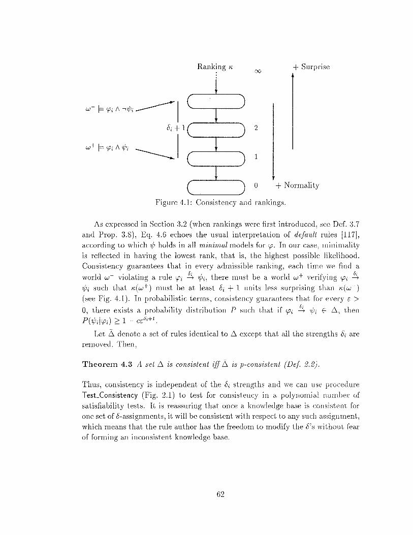![rp) > 8 is equivalent to K( rp) + 8 < K( •4J 1\ rp) or K( 1/J 1\ rp) + 8 < /\:( •1/J 1\ rp ), which is precisely the constraint on worlds we attribute to rp ~ 1{!.

Definition 4.2 (Consistency) A ranking K is said to be admissible relative to a given .6., iff

(4.6)

(equivalently K( •7f!i [rpi) > 8i) for every rule lpi ~ 7f!i E .6.. A knowledge base .6. is consistent iff there exists an admissible ranking K relative to .6..9

D

8 For simplicity we skip the treatment of strict rules. The only necessary change required is in the conditions for admissibility in Def. 4.2. A strict rule </; :::> (J imposes the following admissibility constraint: K((J 1\ </;) < K(-o(J 1\ </;)and K(</;) < oo (see Sec. 5.3, Eq. 5.8).

9 Definition 4.2 represents the ranking equivalent of consistency and admissibility in Defini­tion 3.2 (and Prp. 3.8) with a slight generatlization due to the new parameter 8. For reasons of simplicity I chose not to introduce a new term such as "K-consistency". Also, as shown in Theorem 4.3 both notions are tested using the same procedure: Procedure Test_ Consistency.

61

Ranking K 00

+ Surprise

2

1

0 + Normality

Figure 4.1: Consistency and rankings.

As expressed in Section 3.2 (when rankings were first introduced, see Def. 3. 7 and Prop. 3.8), Eq. 4.6 echoes the usual interpretation of default rules [117], according to which 7/J holds in all minimal models for zp. In our case, minimality is reflected in having the lowest rank, that is, the highest possible likelihood. Consistency guarantees that in every admissible ranking, each time we find a

world w- violating a rule I.Pi ~ 7/Ji, there must be a world w+ verifying I.Pi ~ 7/Ji such that K(w+) must be at least 8i + 1 units less surprising than K(w-) (see Fig. 4.1). In probabilistic terms, consistency guarantees that for every c > 0, there exists a probability distribution P such that if I.Pi ~ 7/Ji E 6, then P(7/Jiii.Pi) 2::1- cc5i+1

.

Let l. denote a set of rules identical to 6 except that all the strengths 8i are removed. Then,

Theorem 4.3 A set 6 is consistent iff l. is p-consistent {Def. 2.2).

Thus, consistency is independent of the 8i strengths and we can use procedure Test_ Consistency (Fig. 2.1) to test for consistency in a polynomial number of satisfiability tests. It is reassuring that once a knowledge base is consistent for one set of 8-assignments, it will be consistent with respect to any such assignment, which means that the rule author has the freedom to modify the 8's without fear of forming an inconsistent knowledge base.

62

4.3 Plausible Conclusions: The z+ -Rank

Given a set 6., each admissible ranking K induces a consequence relation ~'

where <jJ ~ O" iff K(O" 1\ <jl) < K(-,0" 1\ </J). A straightforward way to declare O" as a plausible conclusion of 6. given <jJ would be to require <jJ ~ O" in all rv admissible with 6. However, this will result in an entailment relation equivalent to p­entailment which was shown to be too conservative (Chap. 3). Thus, similar to the approach taken in Chapter 3, we select a distinguished admissible ranking, rv+, and declare O" as a plausible conclusion of 6. given </l, written <jJ f+ /, iff rv+(<jl 1\ O") < K+(<jl 1\ -,0"). 10

The ranking rv+ assigns to each world the lowest possible rank permitted by the admissibility constraints of Eq. 4.6. We will first introduce a syntactic definition of rv+ and then show that it satisfies the desired minimality condition.

Definition 4.4 (The ranking K+) Let 6. = { 1'; I ri = !..pi ~ ?,Vi} be a consistent set of rules. rv+ is defined as follows:

{

0 if w does not falsify any rule in .6. rv+(w) =

maxwf=<p;A-.,;,;[Z+(ri)] + 1 otherwise

where z+(ri) is a priority ordering on rules, defined by

0

(4.7)

(4.8)

Eqs. 4. 7 and 4.8 can be viewed as two coupled equations; one defines rv+ in terms of z+, the second defines z+ in terms of rv+. Figure 4.2 presents an effective procedure, procedure z+ _order, for computing z+ from 6.. The significance of Eq. 4.8 is that the priorities function z+ constitute an economical way of encoding the ranking K+, linear in the size of .6., from which the rv+ of any world w can be computed by searching the highest z+ rule violated by win a logarithmic number (on the number of rules in .6.) of satisfiability tests. The resulting consequence relation f+ and its associated reasoning procedures are called system-z+.

We next show (Thm. 4. 7 and Cor. 4.8) that Eqs. 4. 7 and 4.8 define a unique admissible ranking function rv+ that is minimal in the following sense: Any other admissible ranking function must assign a higher ranking to at least one world and

10If we are concerned with the strength {j with which the conclusion is endorsed, then rj; I~ 1 iff {j is the lowest (positive) integer I satisfying tc+ ( rj; /\ O") + I < tc+ ( rj; /\ •O").

63

a lower ranking to none. To make the result formal, we introduce the following definitions:

Definition 4.5 (Minimal ranking) A ranking function K, is said to be minimal

if every other admissible ranking K, 1 satisfies K, 1 ( w) > K, ( w) for at least one possible

world w. 0

Definition 4.6 (Compact rankings) An admissible ranking "' 1s said to be compact if, for every w' any ranking K, 1 satisfying

is not admissible. 0

K,'(w) K,(w) w "/= w'

K1(w) < K(w) w = w'

Theorem 4. 7 Every consistent 6. has a unique compact ranking given by "'+.

Corollary 4.8 Every consistent 6. has a unique minimal ranking given by K,+.

Note the similarity between k+ (Eq. 4. 7) and the ranking k* associated with the maximum entropy approach (reproduced below)

{

0 if w does not falsify any rule in 6., K,*(w) =

L.".::wF'PiA-,p;[Z*(r;)] + 1 otherwise. (4.9)

While "'+ ( w) is defined by the maximum-priority rule violated in w, K,* ( w) depends on the summation of these priorities. This difference will have implications for both the computational complexity and the quality of conclusions that these two proposals sanction.

The computation of the Z* priorities and the query-answering procedures for the maximum entropy approach has been proven to be NP-hard even for Horn clauses (see [9]). In contrast, the computation of z+ using Procedure z+ _order can be accomplished 0(16.1 2 x log 16.1) satisfiability tests ('I'hm L1. 12). The procedure for computing z+ is presented in Figure 4.2, and is very similar to the one in Figure 3.1. Some of the steps in procedure z+ _order invoke a test of toleration (Def. 2.3). A rule <P !_, O" is tolerated by 6. if the wff <P 1\ O" Ai 'Pi ::::> 'lj;;

is satisfiable (where i ranges over all rules in 6.).

Theorem 4.9 establishes the correctness of procedure z+ _order, while Lem­mas 4.10 and 4.11 and Theorem 4.12 determine its (polynomial) complexity.

64

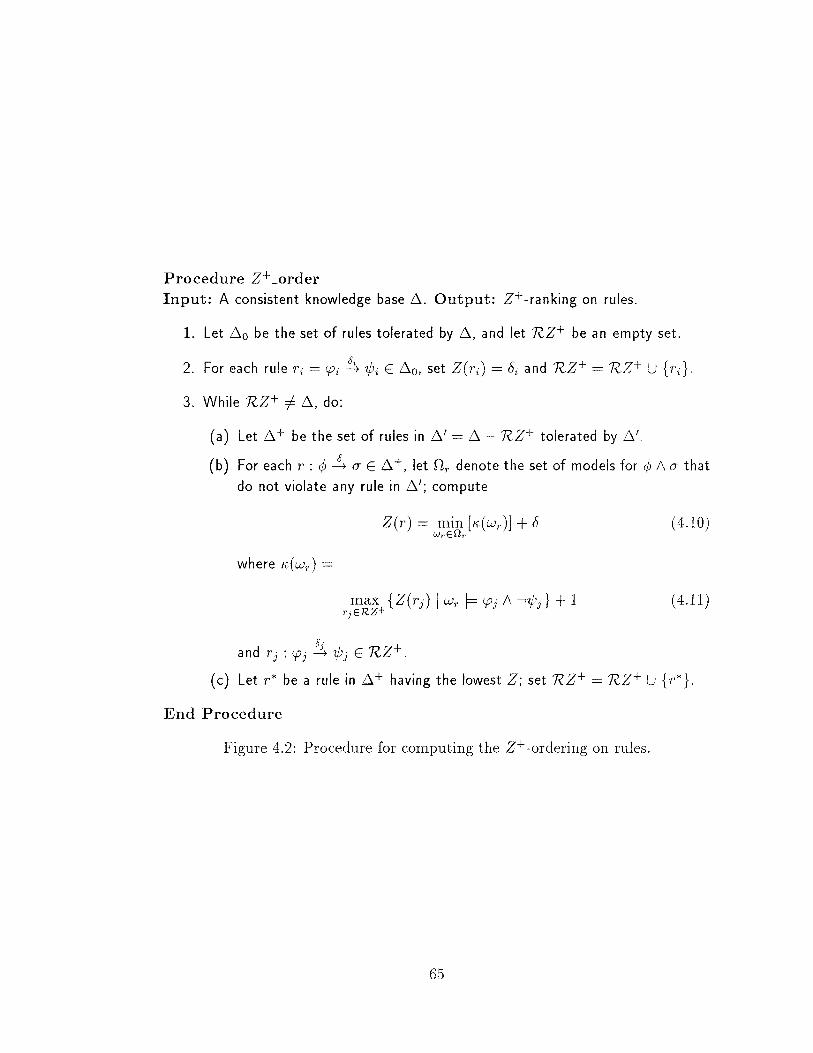
Procedure z+ _order Input: A consistent knowledge base .6.. Output: z+ -ranking on rules.

1. Let .6.0 be the set of rules tolerated by .6., and let nz+ be an empty set.

2. For each rule Ti = lpi ~ 'lj;i E .6.o, set Z(ri) = Di and nz+ = nz+ u {ri}.

3. While nz+ -f- .6., do:

(a) Let .6. + be the set of ruies in .6.' = .6. - nz+ toierated by .6.'.

(b) For each r : cj; _!_, a E .6. +, let Dr denote the set of models for ¢; 1\ a that do not violate any rule in .6.'; compute

Z(r) = min [K(wr)] + 8 WrEilr

where K(wr) =

(4.11)

and Tj : lpj ~ 'lj;j E nz+. (c) Let r* be a rule in .6_+ having the lowest Z; set nz+ = nz+ u {r*}.

End Procedure

Figure 4.2: Procedure for computing the z+ -ordering on rules.

65

Theorem 4.9 The function Z computed by procedure z+ _order satisfies Def. 4-4~ that is z = z+ _11

Lemma 4.10 Let L1 = {r; I r; = 'Pi ~ 7;6;} be a consistent knowledge base in which rules are sorted according a priority function Z (ri). Let ~>:( w) be defi:ned as in Eq. 4. 7:

{

0 if w does not falsify any rule in Ll 1

~>:(w) =

maxwp<p;/\--.,P; [Z(ri)] + 1 otherwise. ( 4.12)

Then1 for any wff <P~ ~>:( <P) can be computed in O(log jill) propositional satisfiability tests.

The idea is to perform a binary search on L1 to find the lowest Z ( r) such that there is a model for <P that does not violate any ruler' with priority Z(r') 2: Z(r). This is done by dividing L1 into two roughly equal sections: top-half (rmid to Thigh) and bottom-half (rzow to rmiJ). A satisfiability test on the wff o: = <P 1\j~~,id yj :::::> 7/'j

decides whether the search should continue (in a recursive fashion) on the bottom­half or top-half.

Lemma 4.11 The value ofZ(<P !._,a) in Eq. 4.10 can be computed in O(log jnz+j) satisfiability tests.

Let 6.' in Step 3( a) of procedure z+ _order be equal to {'Pi ~ 7/'i}; the computation

of Eq. 4.10 is equivalent to computing the K of the wff a A <P 1\i 'Pi :::::> ·1f!i where i ranges over all the rules in 6.' by performing the binary search on the set nz+.

Theorem 4.12 Given a consistent 6. 1 the computation of the ranking z+ re­quires 0(16.1 2 x log j6.j) satisfiability tests.

Computing Eq. 4.10 in Step 3(b) can be done in O(log jnz+j) satisfiability tests according to Lemma 4.11,12 and, since it will be executed at most 0(16.1) times, it requires a total of 0(16.1 x log 16.1). Loop 3 is performed at most 161 - j6.0 j

11 Note that Eqs. 4.10 and 4.11 correspond to Eqs. 4.8 and 4.7 in Def. 4.4. 12 Note that we need nz+ to be sorted, nondecreasingly, with respect to the priorities Z.

This requires that the initial values inserted in nz+ in Step 2 of procedure z+ _order be sorted taking O(IL}.0 1

2 ) data comparisons and that the new Z-value in Step 3(c) be inserted in the right place taking 0( IRZ+ I) data comparisons. We are assuming that the cost of each of these operations is much less than that of a satisfiability test.

66

times, hence the whole computation of the priorities z+ on rules requires a total of 0(16.1 2 x log 16.1) satisfiability tests. 13

Once z+ is known, determining the strength 8 with which an arbitrary query(}' is confirmed, given the information r/J, requires O(log 16.1) satisfiability tests: First K+ ( rP A 0') and K+ ( rP A -,0') are computed, using a binary search as in Lemma 4.10. Then, these two values are compared and the difference is equated with the strength 8. Clearly, if the rules in 6. are of Horn form, computing the prior­ity ranking z+ and deciding the plausibility of queries ( rP rf (}') can be done in polynomial time (2.5].

In the special case of a fiat 6., that is, all 8's = 0, the procedure reduces to the following steps: First, identify all rules ri : !.f!i -+ 'lj;i in 6. for which the formula

!.f!i A 'lj;i 1\ !.f!j :::> 'lj;j (4.13) ji:.i,rjE!:::.

is satisfiable. Next, assign to these defaults priority z+ = 0, remove them from 6., and repeat the process, assigning to the next set of defaults the priority z+ = 1, then z+ = 2, and so on. Once z+ is known, the rank A:+ of any wff rP is given by K+(rP) = minimum i, such that

rP 1\ c.p j :::> 7/'j ( 4.14) j:Z+(r1 ):2:i

is satisfiable. This special case of a fiat 6. constitutes system-Z as introduced by Pearl [100].

An important result implied by Eqs. 4.13 and 4.14 gives a method of con­structing a propositional theory T h( rP) that implies all the conclusions 0' that plausibly follow from a given evidence r/J, that is, rP f+ 0'. Such a theory is given by the formula

Th(r/J)= (4.1.5)

This is somewhat reminiscence of Brewka's [16] and Poole's [104] idea. of con­structing preferred subtheories that are maximally consistent with the context rjJ. Here , the construction is more cautious; it stops as soon as all rules of priority z+ 2: A:+ ( rP) are included in the theory. Ways of completing the construction were proposed by Boutilier [1.5] (see discussion in Sec. 4.7). Note, however, that in contrast to Brewka's and Poole's proposals, our priorities are computed auto­matically from the knowledge base.

13The complexity of the rest of the steps in the procedure is bounded by O(J~i) satisfiability tests.

67

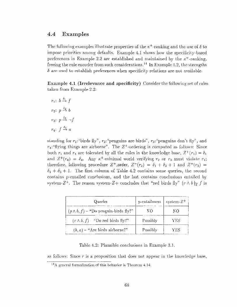
4.4 Examples

The following examples illustrate properties of the ~>:+-ranking and the use of 5 to impose priorities among defaults. Example 4.1 shows how the specificity-based preferences in Example 2.2 are established and maintained by the ~>:+-ranking, freeing the rule encoder from such considerations. 14 In Example 4.2, the strengths 5 are used to establish preferences when specificity relations are not available.

Example 4.1 (Irrelevance and specificity) Consider the following set of rules taken from Example 2.2:

1'1: b~f

r2: 02 b p---+

r3: 03 f p---+•

r4: f 04 ---+a

standing for r 1:"birds fly", r 2:"penguins are birds", r 3:"penguins don't fly", and r 4 : "flying things are airborne". The z+ -ordering is computed as follows: Since both r 1 and r 4 are tolerated by all the rules in the knowledge base, z+ ( ri) = 51

and z+(r4) = 54. Any ~>:+-minimal world verifying r2 or r3 must violate r1; therefore, following procedure z+ _order, z+(r2) = 51 + 52 + 1 and z+(r3) =

51 + 53 + 1. The first column of Table 4.2 contains some queries, the second contains p-entailed conclusions, and the last contains conclusions entailed by system-z+. The reason system-Z+ concludes that "red birds fly" (r 1\ b f+ f is

Queries p-entailment system-z+

(p 1\ b, f)- "Do penguin-birds fly?" NO NO

(rl\b,J) "Do red birds fly?" Possibly YES

(b,a)- "Are birds airborne?" Possibly YES

Table 4.2: Plausible conclusions in Example 3.1.

as follows: Since 1· is a proposition that does not appear in the knowledge base,

14 A general formalization of this behavior is Theorem 4.14.

68

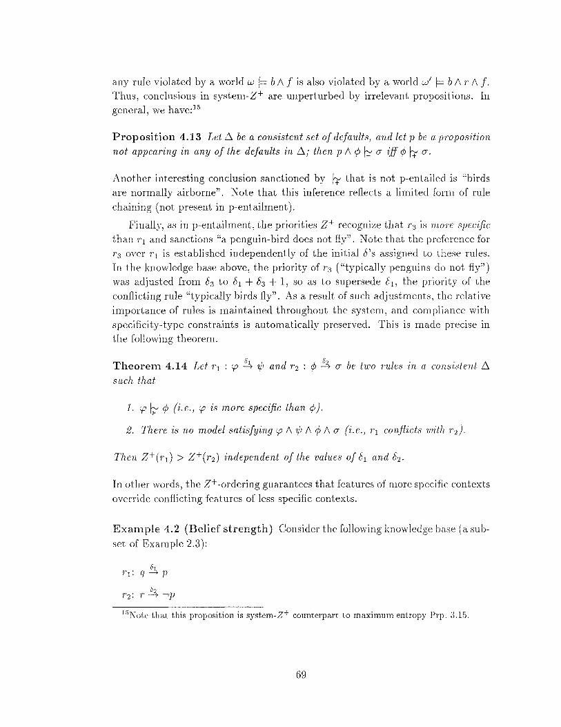
any rule violated by a world w f= b 1\ f is also violated by a world w' b 1\ r 1\ f. Thus, conclusions in system-z+ are unperturbed by irrelevant propositions. In general, we have: 15

Proposition 4.13 Let~ be a consistent set of defa1tlts1 and let p be a proposition

not appearing in any of the defaults in ~; then p 1\ ¢ rr (}" iff¢ rr (}". Another interesting conclusion sanctioned by rr that is not p-entailed is "birds are normally airborne". Note that this inference reflects a limited form of rule chaining (not present in p-entailment ).

Finally, as in p-entailment, the priorities z+ recognize that r3 is more specific

than r 1 and sanctions "a penguin-bird does not fly". Note that the preference for r 3 over r 1 is established independently of the initial 8's assigned to these rules. In the know ledge base above, the priority of r 3 ("typically penguins do not fly") was adjusted from 83 to 81 + 83 + 1, so as to supersede 81 , the priority of the conflicting rule "typically birds fly". As a result of such adjustments, the relative importance of rules is maintained throughout the system, and compliance with specificity-type constraints is automatically preserved. This is made precise in the following theorem.

Theorem 4.14 Let r 1 : <p ~ '1/J and r 2 : ¢ !4 O" be two rules in a consistent ~ such that

1. <p ~ ¢ (i.e. 1 <pis more specific than¢).

2. There is no model satisfying <p 1\ '1/J 1\ ¢ 1\ O" (i.e. 1 r 1 conflicts with r- 2 ).

Then z+(r-I) > z+(r-2 ) independent of the values of 81 and 82.

In other words, the z+ -ordering guarantees that features of more specific contexts override conflicting features of less specific contexts.

Example 4.2 (Belief strength) Consider the following knowledge base (a sub­

set of Example 2.3):

15 Note that this proposition is system-z+ counterpart to maximum entropy Prp. 3.15.

69

standing for ry "typically Quakers are pacifists" and r 2 : "typically Republicans are not pacifists". Since each rule is tolerated by the other, the z+ of each rule is

equal to its associated 8: z+(r1 ) = 81 and z+(r2) = 82 . Given an individual, say Nixon, who is both a Republican and a Quaker, the decision of whether Nixon is

a pacifist will depend on whether 81 is larger than, less than, or equal to 82 . This is because any model Wrqp for Quakers, Republicans, and pacifists must violate r 2 ,

and consequently ~>;+(wrqp) = 82, while any modelwrq~p for Quakers, Republicans, and non-pacifists must violate r1, that is, ~>;+(wrq~p) = 81 • In this case the decision

to prefer one world over the other does not depend on specificity considerations but rather on whether the rule encoder believes that religious convictions carry

more weight than political affiliations.

The main shortcomings of system-z+ are discussed in Sections 3.4 and 4. 7.

4.5 Belief Change, Soft Evidence, and Imprecise Obser­vations

So far, a query <jJ f{ a was defined as a pair of Boolean formulas ( <jJ, O"), where

<jJ (the context) stands for the set of observations at hand and O" (the target) stands for the conclusion whose belief we wish to confirm, deny, or assess. A

query ( </J, a) would be answered in the affirmative if a was found to hold in all

minimally ranked models of </J, and the degree of belief in a would be given by

~>;( •O" 1\ <P) -~>;(a 1\ <P ).

In many cases, however, the queries we wish to answer cannot be cast in this format, because our set of observations is not precise enough to be articulated as a

crisp Boolean formula. For example, assume that we are throwing a forrnal party

and our friends Mary and Bill are invited. However, judging from their previous

behavior, we believe "if Mary goes to the party, Bill will stay home (with strength

8)", written M _!__. •B. Now assume that we have a strong hunch (with degree

K) that Mary will go to the party (perhaps because she is extremely well dressed

and is not consulting the movie section in the Times) and we wish to inquire

whether Bill will stay home. It would be inappropriate to query the system

with the pair (NI, •B), because the context M has not been established beyond doubt. The difference could be critical if we have arguments against "Bill staying

home", (e.g., he was seen renting a tuxedo). A flexible system should allow the user to assign a degree of belief to each observational proposition in the context

<jJ and proceed with analyzing their rational consequences. Thus, a. query should

consist of a tuple like (¢Jl,Kl;¢J2,K2; ... ,</Jm,Km: a), where each Ki measures

70

the degree to which the contextual proposition ¢; is supported by evidence. 16

At first glance it might seem that system-z+ would automatica.lly provide

such a facility through the use of variable-strength rules. For example, to express the fact that Mary is believed to be going to the party, we can perhaps use a

dummy rule Obs1 !!..r M (stating that if Mary meets the set of observations Obs1 ,

then Mary is believed to be going to the party) and then add the proposition

Obs1 to the context part of the query, to indicate that Obs1 has taken place.

This proposal has several shortcomings, however. First, in many systems it

is convenient to treat if-then rules as a stable part of our knowledge, unper­

turbed by observations made about a particular individual or in any specific set of circumstances. This permits us to compile rules into a structure that allows

efficient processing over a long stream of queries. Adding query-induced rules to

the knowledge base will neutralize this facility.

Second, rules and observations combine differently: The latter should accu­

mulate, the former do not. For example, if we have two rules a~ c and b ~ c and

we observe a and b, system-z+ would believe c to a degree max(81 , 82 ). However, if a and b provide two independent reasons for believing c, the two observations together should endow c with a belief that is stronger than any one component

in isolation. To incorporate such cumulative pooling of evidence, we must encode

the assumption that a and bare conditionally independent (given c), which is not automatically embodied in system-z+ _17

To avoid these complications, the method we propose treats imprecise obser­

vations by invoking specialized conditioning operators, unconstrained by a rule's semantics. We distinguish between two types of evidential reports:

1. Type-J: "All things considered," our current belief in ¢should become J.

2. Type-1: "Nothing else considered," our current belief in ¢ should shift by

L. 16Wc rcmark that cvidcncc in this dissertation is rcgardcd as sctting thc context of a qucry

and not as a modifier of the knowledge in t.. Statistical methods for accomplishing the latter task arc explored by Bacchus [6].

17The assumptions of conditional independence among converging rules is embodied in the formalism of rnaximum entropy (see Chapter 3 and [47]), as well as in the causal interpretation of Chapter 5.

71

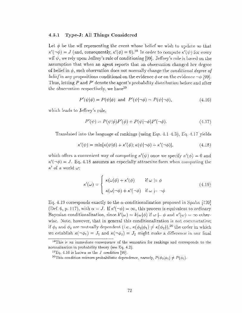
4.5.1 Type-J: All Things Considered

Let 4; be the wff representing the event whose belief we wish to update so that

K,1(•o/) = J (and, consequently, K,

1(o/) = 0). 18 In order to compute K'(<f;) for every wff ~p, we rely upon Jeffrey's rule of conditioning [99]. Jeffrey's rule is based on the assumption that when an agent reports that an observation changed her degree of belief in 4;, such observation does not normally change the conditional degree of beliefin any propositions conditional on the evidence 4; or on the evidence •o/ [99]. Thus, letting P and P' denote the agent's probability distribution before and after the observation respectively, we have19

( 4.16)

which leads to Jeffrey's rule,

( 4.17)

Translated into the language of rankings (using Eqs. 4.1-4.3), Eq. 4.17 yields

(4.18)

which offers a convenient way of computing K,1

( </;) once we specify K,1

( ¢) = 0 and K,

1(•4;) = J. Eq. 4.18 assumes an especially attractive form when computing the K,

1 of a world w:

if w F= q;

if w F= .q;

Eq. 4.19 corresponds exactly to the a-conditionalization proposed in Spohn [120] (Def. 6, p. 117), with a= J. If K,

1( •¢) = oo, this process is equivalent to ordinary

Bayesian conditionalization, since k'(w) = k(wjc/;) if w f= ¢and K'(w) = oo other­wise. Note, however, that in general this conditionalization is not commutative; if (hand o/2 are mutually dependent (i.e., K,(o/214;1) =f. K,(¢2)), 20 the order in which we establish K,( •o/1) = J1 and K,( •o/2) = J2 might make a difference in our final

18This is an immediate consequence of the semantics for rankings and corresponds to the normalization in probability theory (see Eq. 4.2).

19 Eq. 4.16 is known as the ]-condition [99]. 20This condition mirrors probabilistic dependence, namely, P(¢2 1¢1) # P(¢2 ).

72

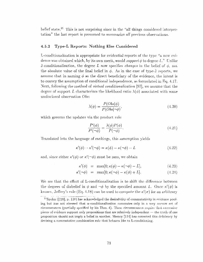
belief state. 21 This is not surprising since in the "all things considered interpre­tation" the last report is presumed to summarize all previous observations.

4.5.2 Type-L Reports: Nothing Else Considered

L-conditionalization is appropriate for evidential reports of the type "a new evi­dence was obtained which, by its own merit, would support <P to degree L." 1Jnlike J-conditionalization, the degree L now specifies changes in the belief of </J, not the absolute value of the final belief in </J. As in the case of type-J reports, we assume that in naming <P as the direct beneficiary of the evidence, the intent is to convey the assumption of conditional independence, as formulated in Eq. 4.17. Next, following the method of vi1'tual conditionalization [97], we assume that the degree of support L characterizes the likelihood-ratio A( <P) associated with some undisclosed observation Obs:

)., ( <P) _ P ( 0 bs I <P) - P(Obsi•<P)'

which governs the updates via the product rule

P'( <P)

P'(•<P) ).,(<jJ)P(<jJ)

P(•<P) .

Translated into the language of rankings, this assumption yields

and, since either "'' ( <P) or "'' ( •<P) must be zero, we obtain

max[O; "'(rP)- "'(•<P)- L],

max[O; "'( •<P) - "'( <P) + L].

(4.20)

( 4.21)

( 4.22)

(4.23)

(4.24)

We see that the effect of L-conditionalization is to shift the difference between the degrees of disbelief in <P and •<P by the specified amount L. Once "'' ( <P) is known, Jeffrey's rule (Eq. 4.18) can be used to compute the"''( cr) for an arbitrary

21 Spohn ([120), p. 118) has acknowledged the desirability of commutativity in evidence pool­ing but has not stressed that n:-conditionalization commutes only in a very narrow set of circumstances (partially specified by his Thm. 4). These circumstances require that successive pieces of evidence support only propositions that are relatively independent - the truth of one proposition should not imply a belief in another. Shenoy [114] has corrected this deficiency by devising a commutative combination rule that behaves like to 1-conditioning.

73

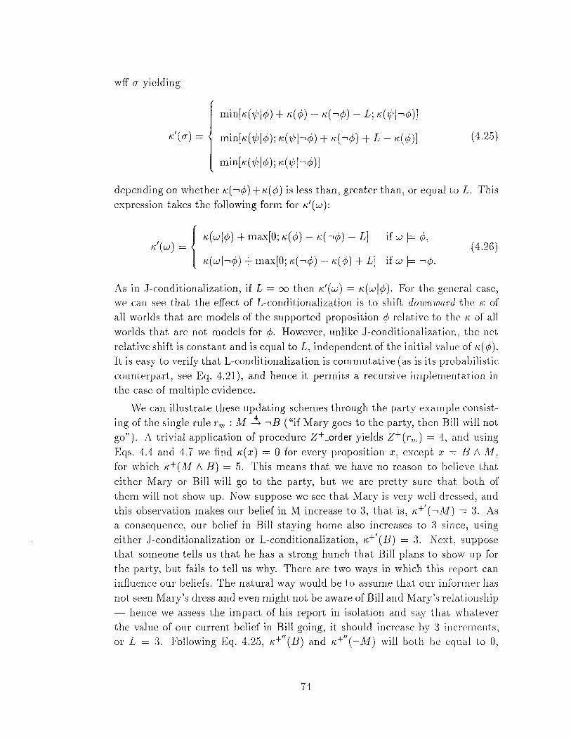
wff cr yielding

r K'(a) = 1

min[!i:(V'icP) +A:(¢)- A:(•¢)- L; A:(~J·¢)]

min[A:(~J¢); !i:(~J·¢) + A:(•¢) +L-A:(¢)]

min[!i:(~J¢); A:(~J·¢)]

( 4.25)

depending on whether A:( •¢) +A:(¢) is less than, greater than, or equal to L. This expression takes the following form for 1\:

1 ( w):

{

A:(wJ¢) + max[O; A:(¢)- A:(•¢)- L] !i:'(w) =

i'C(wJ-.¢) + max[O; I'C(•¢)- i'C(¢) + L]

if w I= ¢,

if w I= •¢.

As in J-conditionalization, if L = oo then A: 1(w) = A:(wJ¢). For the general case, we can see that the effect of 1-conditionalization is to shift downward the A: of all worlds that are models of the supported proposition ¢ relative to the A: of all worlds that are not models for ¢. However, unlike J-conditionalization, the net relative shift is constant and is equal to L, independent of the initial value of i'C( ¢ ). It is easy to verify that 1-conditionalization is commutative (as is its probabilistic counterpart, see Eq. 4.21), and hence it permits a recursive implementation in the case of multiple evidence.

We can illustrate these updating schemes through the party example consist­ing of the single rule r m : M ~ ·B ("if Mary goes to the party, then Bill will not go"). A trivial application of procedure z+ _order yields z+(rm) = 4, and using Eqs. 4.4 and 4. 7 we find A:( x) = 0 for every proposition x, except x = B 1\ Jl,;f,

for which A:+(M 1\ B) = 5. This means that we have no reason to believe that either Mary or Bill will go to the party, but we are pretty sure that both of them will not show up. Now suppose we see that Mary is very well dressed, and this observation makes our belief in M increase to 3, that is, i'C+' ( •1\1) = 3. As a consequence, our belief in Bill staying home also increases to 3 since, using either J-conditionalization or 1-conditionalization, A:+' (B) = 3. Next, suppose that someone tells us that he has a strong hunch that Bill plans to show up for the party, but fails to tell us why. There are two ways in which this report can influence our beliefs. The natural way would be to assume that our informer has not seen Mary's dress and even might not be aware of Bill andl\llary's relationship - hence we assess the impact of his report in isolation and say that whatever the value of our current belief in Bill going, it should increase by 3 increments, or L = 3. Following Eq. 4.2.5, K+" (B) and A:+" ( •M) will both be equal to 0,

74

and we are back to the initial uncertainty about Bill or Mary going to the party, except that our disbelief in both Mary and Bill being at the party has decreased to /\:+" (M 1\ B) = 2. A second way would be to assume that our informer is omniscient and already has taken into consideration all we know about Bill and Mary. He means for us to revise our rankings so that the final belief in "Bill going" will be fixed at /\:+" ( •B) = 3. \iVith this interpretation, we J-condition /\:+' on the proposition <P = ·B and obtain /\:+" (M) = 3, concluding that it is Mary who will not show up to the party after all.

4.5.3 Complexity Analysis

}'rom Eq. 4.18 we see that I'C'('l/;) can be computed from I'C('l/;j<jJ) and i>:(v,l•¢), which, assuming we have z+, requires a logarithmic number of propositional satisfiability tests (see Sec. 4.3). 1-conditionalization can follow a similar route (see Eq. 4.25).

Special precautions must be taken when simultaneous, multiple pieces of ev­idence become available. First, J-conditionalization is not commutative, hence we cannot simply compute 1\:

1 by ]-conditioning on ¢1 and then ]-conditioning 1\:1

on ¢2 to get 1\:11

• We must J-condition simultaneously on </J1 and ¢2 with their re­spective J-levels, say ] 1 and ] 2 • Worse yet, an auxiliary effort must be expended to compute the J-level of each combination of q)'s, in our case ¢1 1\ ¢2 , ¢1 1\ •¢2 ,

etc. This is no doubt a hopeless computation when the number of observations is large.

1-conditionalization, by virtue of its commutativity, enjoys the benefits of recursive computations. Let e1 and e2 be two (undisclosed) pieces of evidence supporting ¢1 (with strength L1 ) and ¢2 (with strength L2 ), respectively. We first 1-condi tion I'C on ¢1 and calculate 1\:

1 ( ¢1 ) and K

1 ( ¢2 ) using Eq. 4. 24 and

Eq. 4.25, respectively. Applying Eq. 4.25 this time to K/( 'lj; 1\ ¢2 ), we calculate K

1( 'l/;j¢2 ). Second, we L-condition 1\:

1 on ¢2 , compute K11

( ¢2 ) using Eq. 4.24, and finally, using K1('l/;j¢2 ) and K"(¢2 ) in Eq. 4.25 obtain K"('l/;). 22 Note that, aJthough each of these calculations requires only O(log j6j) satisfiability tests, this com­putation is effective only when we have a well designated target hypothesis CJ

to estimate. The computation must be repeated each time we change the tar­get hypothesis, even when the context remains unaltered. This is because we no longer have a facility for economically encoding a complete description of K

1,

as we had for K (using the z+-function). Thus, the encoding for r;,' may not be as economical as that for K (the number of worlds is astronomical), unless

22The generalization to more than two pieces of evidence is straightforward.

75

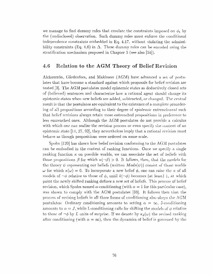
we manage to find dummy rules that emulate the constraints imposed on c/J1 by the (undisclosed) observation. Such dummy rules must enforce the conditional independence constraints embedded in Eq. 4.17, without violating the admissi­bility constraints (Eq. 4.6) in ~. These dummy rules can be encoded using the stratification mechanism proposed in Chapter 5 (see also [54]).

4.6 Relation to the AGM Theory of Belief Revision

Alchourr6n, Giirdenfors, and Makinson (AGM) have advanced a set of postu­lates that have become a standard against which proposals for belief revision are tested [3]. The AGM postulates model epistemic states as deductively closed sets of (believed) sentences and characterize how a rational agent should change its epistemic states when new beliefs are added, subtracted, or changed. The central result is that the postulates are equivalent to the existence of a complete preorder­ing of all propositions according to their degree of epistemic entrenchment such that belief revisions always retain more entrenched propositions in preference to less entrenched ones. Although the AGM postulates do not provide a calculus with which one can realize the revision process or even specify the content of an epistemic state [14, 27, 92], they nevertheless imply that a rational revision must behave as though propositions were ordered on some scale.

Spohn [120] has shown how belief revision conforming to the AGM postulates can be embodied in the context of ranking functions. Once we specify a single ranking function "' on possible worlds, we can associate the set of beliefs with those propositions (3 for which "'( •(3) > 0. It follows, then, that the models for the theory 'ljJ representing our beliefs (written Mods( 'ljJ)) consist of those worlds w for which "'(w) = 0. To incorporate a new belief c/J, one can raise the K of all models of •c/J relative to those of c/J, until k(•c/J) becomes (at least) 1, at which point the newly shifted ranking defines a new set of beliefs. This process of belief revision, which Spohn named a-conditioning (with a= 1 for this particular case), was shown to comply with the AGM postulates [33]. It follows then that the process of revising beliefs in all three forms of conditioning also obeys the AGM postulates: Ordinary conditioning amounts to setting a = oo, J-conditioning

amounts to a = J, while L-conditioning calls for shifting the models of cjJ relative to those of •c/J by L units of surprise. If we denote by K¢( w) the revised ranking after conditioning (with a = oo), then the dynamics of belief is governed by the

76

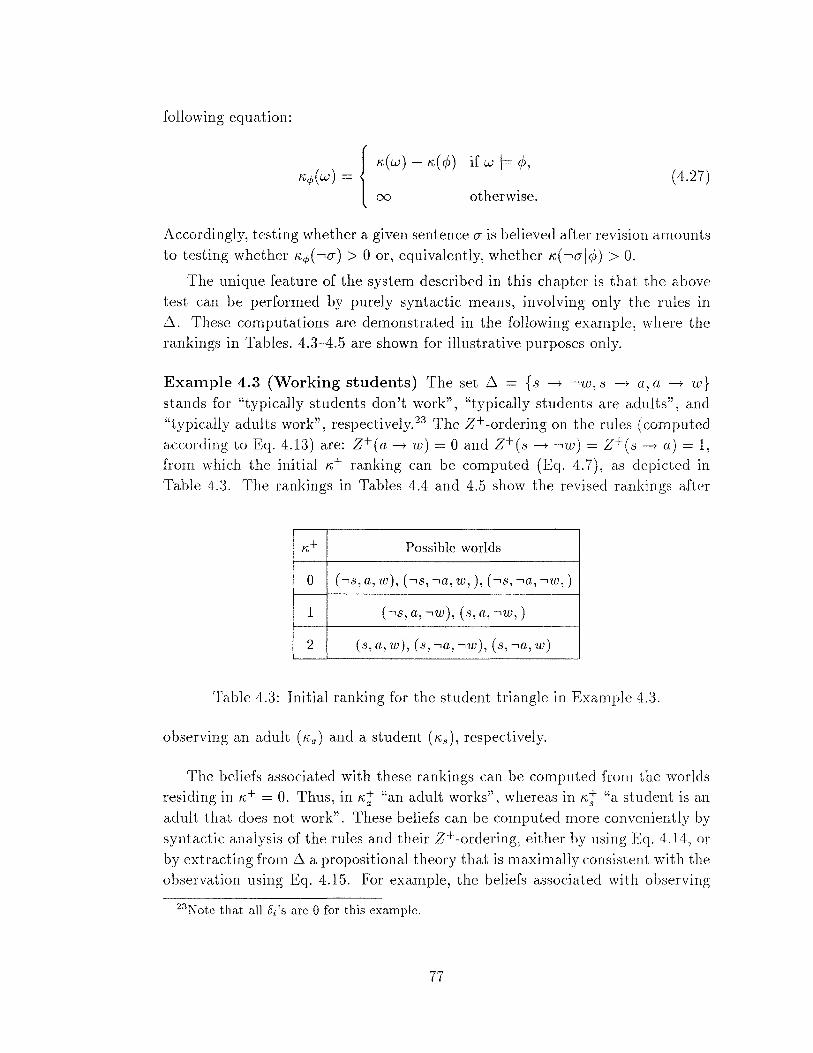
following equation:

"'q,(w) = {

00

"'(w)- "'(¢) if w f= ¢,

otherwise. (4.27)

Accordingly, testing whether a given sentence 0' is believed after revision amounts to testing whether "'¢( •0') > 0 or, equivalently, whether "'( •0'1¢) > 0.

The unique feature of the system described in this chapter is that the above test can be performed by purely syntactic means, involving only the rules in b.. These computations are demonstrated in the following example, where the rankings in Tables. 4.3-4 .. 5 are shown for illustrative purposes only.

Example 4.3 (Working students) The set 6 = { s ---+ •w, s ---+ a, a ---+ w} stands for "typically students don't work", "typically students are adults", and "typically adults work", respectively. 23 The z+ -ordering on the rules (computed according to Eq. 4.13) are: z+(a---+ w) = 0 and z+(s---+ •w) = z+(s---+ a)= 1, from which the initial "'+ ranking can be computed (Eq. 4. 7), as depicted in Table 4.3. The rankings in Tables 4.4 and 4.5 show the revised rankings after

{\,+ Possible worlds

0 ( •s, a, w ), ( •s, •a, w, ), ( •s, •a, ··w,)

1 (•s,a,•w), (s,a,•w,)

2 (s, a, w), (s, •a, •w), (s, •a, w)

Table 4.3: Initial ranking for the student triangle in Example 4.3.

observing an adult ("'a) and a student (Ks), respectively.

The beliefs associated with these rankings can be computed from the worlds residing in "'+ = 0. Thus, in K:;!" "an adult works", whereas in K; "a student is an adult that does not work". These beliefs can be computed more conveniently by syntactic analysis of the rules and their z+ -ordering, either by using Eq. 4.14, or by extracting from 6 a propositional theory that is maximally consistent with the observation using Eq. 4.15. For example, the beliefs associated with observing

23N ote that all 8/s are 0 for this example.

77

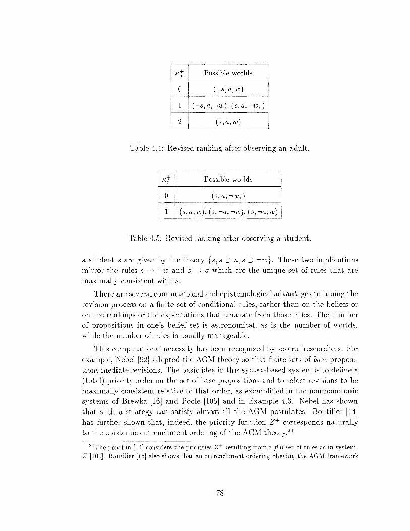
~+ a Possible worlds

0 ( -.s, a, w)

1 ( -.s, a, •w ), ( s, a, •w,)

2 (s,a,w)

Table 4.4: Revised ranking after observing an adult.

+ ~s Possible worlds

0 (s, a, •w,)

1 (s, a, w), (s, -.a, -,w), (s, -,a, w)

Table 4.5: Revised ranking after observing a student.

a student s are given by the theory { s, s ::::> a, s ::::> •w }. These two implications mirror the rules s -+ -,w and s -+ a which are the unique set of rules that are maximally consistent with s.

There are several computational and epistemological advantages to basing the revision process on a finite set of conditional rules, rather than on the beliefs or on the rankings or the expectations that emanate from those rules. The number of propositions in one's belief set is astronomical, as is the number of worlds, while the number of rules is usually manageable.

This computational necessity has been recognized by several researchers. For example, Nebel [92] adapted the AGM theory so that finite sets of base proposi­tions mediate revisions. The basic idea in this syntax-based system is to define a (total) priority order on the set of base propositions and to select revisions to be maximally consistent relative to that order, as exemplified in the nonmonotonic systems of Brewka [16] and Poole [105] and in Example 4.3. Nebel has shown that such a strategy can satisfy almost all the AGM postulates. Boutilier [14] has further shown that, indeed, the priority function z+ corresponds naturally to the epistemic entrenchment ordering of the AGM theory. 24

24The proof in [14] considers the priorities z+ resulting from a fiat set of rules as in system­z [100]. Boutilier [15] also shows that an entrenchment ordering obeying the AGM framework

78

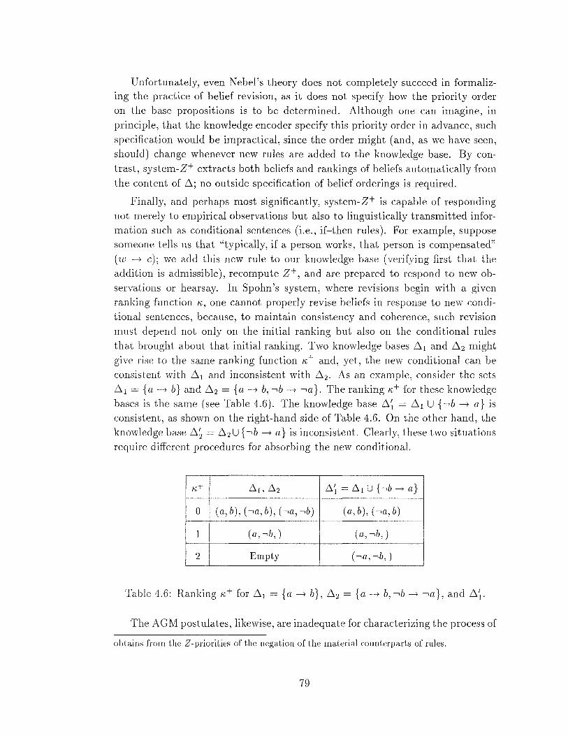
Unfortunately, even Nebel's theory does not completely succeed in formaliz­ing the practice of belief revision, as it does not specify how the priority order on the base propositions is to be determined. Although one can imagine, in principle, that the knowledge encoder specify this priority order in advance, such

specification would be impractical, since the order might (and, as we have seen, should) change whenever new rules are added to the knowledge base. By con­trast, system-z+ extracts both beliefs and rankings of beliefs automatically from

the content of 6; no outside specification of belief orderings is required.

Finally, and perhaps most significantly, system-z+ is capable of responding not merely to empirical observations but also to linguistically transmitted infor­mation such as conditional sentences (i.e., if-then rules). For example, suppose someone tells us that "typically, if a person works, that person is compensated" (w ---+ c); we add this new rule to our knowledge base (verifying first that the addition is admissible), recompute z+, and are prepared to respond to new ob­

servations or hearsay. In Spohn's system, where revisions begin with a given ranking function n,, one cannot properly revise beliefs in response to new condi­tional sentences, because, to maintain consistency and coherence, such revision must depend not only on the initial ranking but also on the conditional rules that brought about that initial ranking. Two knowledge bases 6 1 and 6 2 might give rise to the same ranking function n,+ and, yet, the new conditional can be consistent with 6 1 and inconsistent with 6 2 . As an example, consider the sets 6 1 {a ---+ b} and 6 2 = {a ---+ b, •b ---+ •a}. The ranking n,+ for these knowledge bases is the same (see Table 4.6). The knowledge base 6~ = 6 1 U { -.b ---+ a} is consistent, as shown on the right-hand side of Table 4.6. On the other hand, the knowledge base 6; = 6 2 U { ·b ---+ a} is inconsistent. Clearly, these two situations require different procedures for absorbing the new conditional.

n,+ 61,62 6~ = 6 1 U {•b-+ a}

0 (a, b), (•a, b), (•a,•b) (a, b), (•a,b)

1 (a, •b,) (a, •b, )

2 Empty ( •a, •b,)

Table 4.6: Ranking n,+ for 6 1 ={a---+ b}, 6 2 ={a---+ b, •b---+ -.a}, and 6~.

The AGM postulates, likewise, are inadequate for characterizing the process of

obtains from the Z-priorities of the negation of the material counterparts of rules.

79

incorporating new conditionals, because they are formulated as transformations on belief sets and are thus oblivious to the set of conditionals that shaped those belief sets, and into which the new conditional is about to join.25

The ability to adopt new conditionals (as rules) also provides a simple seman­tics for interpreting nested conditionals (e.g., "if you wear a helmet whenever you ride a motorcycle, then you won't get hurt badly if you fall" 26

). Nested condi­tionals cease to be a mystery once we permit explicit references to default rules. The sentence "If (a ---+ b) then ( c---+ d)" is interpreted as

"If I add the default a ---+ b to E:., then the conditional c ---+ d will be satisfied by the consequence relation rr of the resulting knowledge base E:.' = 6 U {a---+ b}".

which is clearly a proposition that can be tested in the language of default-based ranking systems. Note the essential distinction between having a conditional sentence a ---+ b explicitly in 6 versus having a conditional sentence a ---+ b satisfied by the consequence relation rr of 6. In both cases the conditional a ---+ b would meet the Ramsey test, but only the former case would resist the adoption of the conditional a ---+ •b. This distinction gets lost in systems that do not acknowledge defaults as the basis for ranking and beliefs. 27

4. 7 Discussion

This chapter proposes a belief-revision system that reasons semi-tractably and plausibly with linguistic quantification of both observational reports (e.g., "looks like") and domain rules (e.g., "typically"). The system is semi-tractable in the sense that it is tractable for every sublanguage in which propositional satisfiability is polynomial (Horn expressions, network theories, acyclic expressions, etc.). To the best of my knowledge, this is the first system that reasons with approximate probabilities which offers such broad guarantees of tractability. Whereas most tractability results exploit the topological structure of the knowledge base [20, 71, 97] (hypertrees, or partial hypertrees ), ours are topology-independent. These results should carry over to the theory of possibility as formulated by Dubois and Prade [28], which has similar features to Spohn's system except that beliefs

25 Gardenfors (33, pp. 156-160] attempts to devise postulates for conditional sentences, but finds them incompatible with the Ramsey test.

26Judea Pearl attributes this example to Philip Calabrese (personal communication). 27Belief revision systems proposed in the database literature [31, 19] suffer from the same

shortcoming. In that context, defaults represent integrity constraints with exceptions.

80

are measured on the real interval [0, 1). In addition, as Section 4.5 shows, the system can also accommodate expressions of imprecise observations without loss of tractability, thus providing a good model for weighing the impact of evidence and counter-evidence on our beliefs. Also the enterprise of belief revision, as formulated in the work presented in [3, 33], can find a tractable and natural em­bodiment in system-z+' unhindered by difficulties that plagued earlier systems.

From the perspective of defeasible reasoning, system-z+ provides the user with the power to explicitly set priorities among default rules, and simultane­ously maintains a proper account for specificity relations. However, it inherits some of the deficiencies of system-Z [100] 28 the main one being the inability to sanction inheritance across exceptional subclasses (see Exm. 3.2). To illustrate

this problem consider adding a a fifth rule b ~ l ("birds have legs") to the set of rules in Example 4.1:

r:~: p ·f

r4: f a

rs: b~l

We would normally conclude from this set that "penguins have legs", while system-Z (with fji = 0) will consider "penguins" exceptional "birds" with re­spect to all properties, including "having legs". The K:+ -ranking now allows the rule author to partially bypass this obstacle by adjusting the 8's. If 85 is set to be bigger than 81 (to express perhaps the intuition that anatomic properties are more typical than developmental facilities) then the system will conclude that "typically penguins have legs" .29 This solution however, is not entirely satisfac­tory. If we add to this new set of rules a class of "birds" which are "legless", system-z+ will conclude that either "penguins have legs" or "legless birds fly" but not both. 30 In order to overcome this difficulty, a system must comply with the preference condition in Proposition 3.16. As shown in Section 3.4, maximum

28 And the rational closure described in [72]. 29 Note that the fact that "penguins" are only exceptional with respect "flying" (and not

necessarily with respect to "having legs") is automatically encoded in the z+ ranking by forcing z+(r3) to exceed z+(r1) + bs independently of 65 (and z+(r5)).

30This counterexample is due to Kurt Konolige.

81

entropy is one such system; two other systems that satisfy this result are Geffner's Conditional Entailment [36, 38], and the proposal by Boutilier [15).

In Geffner's conditional entailment, rather than letting rule priorities dictate a ranking function on models, a partial order on interpretations is induced instead. To determine the preference between w and w', we examine the highest priority rules that distinguish between the two, i.e., that are falsified by one and not by the other. If all such rules remain unfalsified in one of the two possible worlds, then this model is the preferred one. Formally, if .F[w) and .F[w') stand for the set

of rules falsified by w and w' respectively, then w is preferred tow' iff .F[w) =f. .F[w'] and for every rule in .F[w)- .F[w'] there exists a rule f' in .F[w')- .F[w] such that f' has a higher priority than f (written f' > f). Thus, a model w will always be preferred to w' if it falsifies a proper subset of the rules falsified by w' (see Prop. 3.16).

Priorities among rules in Geffner proposal differ also from both the proposals in Chapter 3 and this chapter, in that the rule priority relation is a partial order as well. This partial order is determined by the following interpretation of the

rule !f' -+ 1/J: If !f' is all we know, then, regardless of other rules that 6. may contain, we are authorized to assert 1/J. This means that f : !f' -+ 1/J should get a higher priority than any argument (a chain of rules) leading from !f' to -,'ljJ and, more generally, if a set 6.' C 6. does not tolerate f, then at least one rule in 6.' ought to have a lower priority than T. In the example above,31

f 3 : p -+ -.J is not tolerated by the set { f 2 : p -+ b, fl : b -+ f}, hence we must have that f 2 < f 3 or 1~ 2 < r·1 . Similarly, the rule r2 : p -+ b is not tolerated by { f 3 : p -+ -.J, fl : b -+ f} and hence we also have f2 < r 1 or f 3 < fl· This two conditions together with the

transitive properties of <, yield r 2 < r 1 and f 3 < fl· Note that in this partial order r 4 cannot be compared to any of the other rules. In general, we say that a proposition O" is conditionally entailed by 4; (in the context of a set 6.) if O" holds in all the preferred models for 4; induced by every priority ordering admissible for 6. Conditional entailment rectifies many of the shortcommings of system-Z, as well as some weaknesses of the entailment relation induced by maximum entropy. However, having been based on model minimization as well as on enumeration

of subsets of rules, its computational complexity might be overbearing. A proof theory for conditional entailment can be found in [36).

Boutilier [15) proposed a system which combines the priority ordering of system-Z (i.e. the flat version of system-Z+), with Brewka's [16) notion of pre­

ferred subtheories. Thus, whereas system-z+ assigns equal rank to any two

worlds that violate a rule T' with z+(r) = z and no rule of higher z+' the pro-

31 Assuming a flat version where alliJ's are zero.

82

posal in [15] will make further comparisons in terms of rules of lower priority violated in these worlds. In the case above, since any minimal world satisfying p 1\ l must violate a proper subset of the rules violated by any minimal model for p 1\ ....,z, the desired conclusion is certified. These notion are formalized in terms of the modal logic CO* which is semantically related to the probabilistic interpre­tation proposed in this dissertation [14]. Nevertheless, counterintuitive examples to this notion of entailment can be found in [36, 48]. While Boutilier's proposal appears to be simpler than conditional entailment (as it does not require partial orders), its computational effectiveness is yet to be analyzed.

83

CHAPTER 5

Causality

5.1 Introduction

Independently of whether causality is a property of nature or a conceptual con­venience, the organization of knowledge as cause-effect relations is fundamental for tasks of prediction and explanation. This chapter introduces, within the basic framework of ranking systems, a simple mechanism called stratification for the representation of causal relationships, actions, and changes.

The lack of a mechanism for distinguishing causal relationships from other kinds of associations has been a serious deficiency in most nonmonotonic sys­tems [96], the classical illustration of which is given by the now-famous Yale Shooting Problem (YSP) [57]. In its simplified version, the YSP builds the ex­pectation that if a gun is loaded at time t0 and Fred is shot with the gun at time t 1 , Fred should be dead at time t 2 , despite the normal tendency of being alive to persist. Many formulations including circumscription [88], default logic [108], maximum entropy (Chap. 3), system-z+ (Chap. 4), and conditional entailment [36] - do not yield the expected conclusion. Instead they reveal an alternative, perfectly symmetrical version of reality, whereby somehow the gun got unloaded and Fred is alive at time t 2 .

The inclination to choose the scenario in which Fred dies is grounded in no­tions of directionality and asymmetry that are particular to causal relationships. This chapter shows that these notions can be derived from one fundamental prin­ciple, Markov shielding, which can be embodied naturally in preferential model semantics using the device of stratified rankings. Informally, the principle can be stated as follows:

• Knowing the set of causes for a given effect renders the effect independent of all prior events.

In the YSP, given the state of the gun at time t1 , the effect of the shooting can be predicted with total disregard for the gun's previous history.

This chapter proposes a probabilistically motivated, ranked-model semantics

84

for rules of the form "typically, if cause1 and ... and causen, then effect", which incorporates the above principle under the assumption that "causes" precede their "effects". As a by-product, our semantics exhibits another feature characteristic of causal organizations: modularity. Informally,

• Adding rules that predict future events cannot invalidate beliefs concerning previous events.

This is analogous to a phenomena we normally associate with causal mechanisms such as logical gates in electrical circuits, where connecting the inputs of a new gate to an existing circuit does not alter the circuit's behavior [21].

Although several remedies were proposed for the YSP within conventional nonmonotonic formalisms [118, 36, 121, 8, 79], the formalism explored in this chapter seeks to uncover remedies systematically from basic probabilistic princi­ples [97, pp. 509-516]. Incorporating such principles in the qualitative context of world ranking yields useful results on several frontiers. In prediction tasks (such as the YSP), our formalism prunes the undesirable scenarios, without the strong commitment displayed by chronological minimization [118] and without the addition of external causal operators to the conditional interpretation of the rules [36] (see Section 5.3). In abduction tasks (such as when Fred is seen alive at t2 ), our formalism yields plausible explanations for the facts observed (e.g., sim­ilar to [121], the gun must have been unloaded sometime before the shooting at t 1 ). These suggests that the principle of Markov shielding, by being grounded in probability theory (hence in empirical reality), can provide a coherent framework for the many facets of causation found in commonsense reasoning. Moreover, given the connection formed among causation, defaults, and probability, we can now ask not merely how to reason with a given set of causal assertions but also whether those assertions are compatible with a given stream of observations. A framework for explanations is further discussed in Section 5.3.2.

Section 5.3.1 defines a notion of consistency in the context of causal rules, and briefly compares it to the notion of p-consistency introduced in Chapter 2. Section 5.4 demonstrates how rank-based systems can embody and unify the the­ories of belief revision [3] and belief updating [65]. Whereas belief revision deals with new information obtained through new observations in a static world, belief update deals with tracing changes in an evolving world, such as that subjected to the external influence of actions.

As shown in Section 4.6 system-z+ offers a natural embodiment of the prin­ciples of belief revision as formulated by Alchourr6n, Gardenfors and Makinson (AGM) [3], with the additional features of enabling the absorption of new con-

85

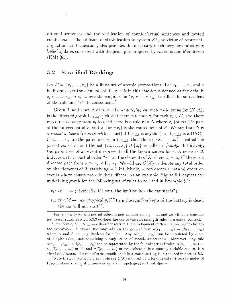
ditional sentences and the verification of counterfactual sentences and nested conditionals. The addition of stratification to system-z+, by virtue of represent­ing actions and causation, also provides the necessary machinery for embodying belief updates consistent with the principles proposed by Katsuno and Mendelzon (KM) [65].

5.2 Stratified Rankings

Let X = { x 1 , ... , x,J be a finite set of atomic propositions. Let c1 , ... , Cm and e be literals over the elements of X. A rule in this chapter is defined as the default c1 1\ ... 1\ Cm -J. e, 1 where the conjunction "c1 1\ ... 1\ Cm" is called the antecedent of the rule a.nd "e" its consequent. 2

Given X a.nd a. set D. of rules, the underlying characteristic graph for (X, D.), is the directed graph r (X,A) such tha.t there is a. node Vi for ea.ch Xi E X' a.nd there is a. directed edge from vi to Vj iff there is a rule r in D. where Xi (or •xi) is part of the antecedent of r, a.nd x j (or •x j) is the consequent of R. We sa.y that D. is a. causal network (or network for short) if r(X,A) is acyclic (i.e., r(X,A) is a DAG). If v,., ... , V 8 a.re the parents of Vt in f (X,A), then the set { Xr, ... , X 8 } is called the parent set of Xt a.nd the set { Xr, ..• , X 8 } U { Xt} is called a. family. Intuitively, the parent set of an event e represents a.ll the known causes for e. A network D. induces a. strict pa.rtia.l order "-<" on the elements of;{' where Xi -< Xj iff there is a. directed pa.th from Vi to Vj in r (X,A). We will use 0( X) to denote a.ny total order on the elements of X satisfying -<.3 Intuitively, -< represents a natural order on events where causes precede their effects. As a.n example, Figure 5.1 depicts the underlying graph for the following set of rules to be used in Example 5.1:

r 1 : tk -J. cs ("typically, if I turn the ignition key the car starts").

r 2 : tk 1\ bd -J. •cs ("typically, if I turn the ignition key a.nd the battery is dead, the ca.r will not start").

1 For simplicity we will not introduce a new connective, e.g. --+c, and we will only consider fiat causal rules. Section 5.3.3 explores the use of variable strength rules in a causal context.

2The form c1 1\ .. . I\ Cm --+ e does not restrict the development of this chapter but it clarifies the exposition. A causal rule may take on the general form a(c1, ... , em) --+ f3(e 1 , ... , en) where a and /3 are any Boolean formulae. Any a( c1 , ... , Cm) can be simulated by a set of simpler rules, each containing a conjunction of atomic antecedents. Moreover, any rule a(c1, ... , em)--+ /3(e1, ... , en) can be represented by the following set of rules: a(c1, ... , em)--+

e', /3( e 1, ... , en) :::> e', and •/3( e 1, ... , en) :::> •e', where e' is a dummy variable and :::> is a strict conditional. The role of strict conditionals in a causal setting is introduced in Section 5.3.

3 Note that, in particular, any ordering O(X) induced by a topological sort on the nodes of f (X C.), where Xi < X j if Vi precedes Vj in the topological sort, satisfies -<.

86

lo

tk bd

cs

Figure 5.1: Underlying graph for the causal rules in the battery example

r 3 : lo -+ bd ("typically, if I leave the headlights on all night the battery is dead").

In previous chapters, the interpretation of a rule <.p -+ 'lj; was based on the condition of admissibility of rc (see Def. 4.2). A ranking rc is admissible relative to ~ iff for every 'Pi -+ 'lj;i E ~:4

(5.1)

We now extend this requirement and introduce a stratification constraint that will endow the rules with a causal character.

Definition 5.1 (Stratified Rankings) Given a network~' an admissible rank­ing rc relative to ~' and an ordering O(X); let Xi (1 ::; i ::; n) denote a lit­eral variable taking values from {Xi, •xi}, and let Par xi denote the conjunction Xr 1\ ... 1\Xs where {Xn ... , Xs} is the parent set of Xi. We say that rc is stratified for ~ under 0( X), if for 2 ::; i ::; n, and for any instantiation of the variables

xl, ... ,xi, we have

(5.2)

0

Eq. 5.2 says that in a stratified ranking the incremental surprise of finding Xi

in a full description of some past scenario, must be equal to the incremental surprise of finding Xi given just the state of Parxi in that same scenario. Thus, the parent set of an event Xi (ParxJ shields this event Xi from all prior events (see Fig. 5.2). This condition parallels the Markovian independence conditions

4 Assuming all O; 's are equal to zero; otherwise admissibility would require that x;( •7/>; !If';) > 8; in Eq.5.1.

87

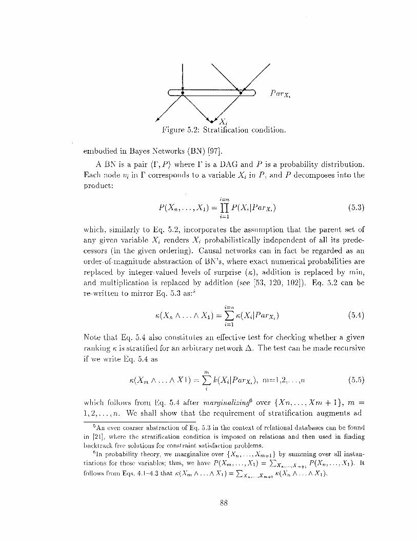
xi Figure 5.2: Stratification condition.

embodied in Bayes Networks (BN) [97).

A BN is a pair (r, P) where r is a DAG and Pis a probability distribution. Each node Vi in r corresponds to a variable xi in p' and p decomposes into the product:

P(Xn, ... , X1) = IJ P(XiiParxJ (5.3) i=l

which, similarly to Eq. 5.2, incorporates the assumption that the parent set of any given variable xi renders xi probabilistically independent of all its prede­cessors (in the given ordering). Causal networks can in fact be regarded as an order-of-magnitude abstraction of BN's, where exact numerical probabilities are replaced by integer-valued levels of surprise ( 11: ), addition is replaced by min, and multiplication is replaced by addition (see [53, 120, 102]). Eq. 5.2 can be re-written to mirror Eq. 5.3 a.s:·5

l=n

~~:(Xn 1\ ... 1\ XI) = L ~~:(XiiParxJ (5.4) i=l

Note that Eq .. 5.4 also constitutes an effective test for checking whether a given ranking 11: is stratified for an arbitrary network 6. The test can be made recursive if we write Eq. 5.4 as

m

~~:(Xm 1\ ... 1\ XI)= L k(XiiParxJ, m=1,2, ... ,n (5.5)

which follows from Eq. 5.4 after marginalizinl over {Xn, ... ,Xm + 1}, m =

1, 2, ... , n. We shall show that the requirement of stratification augments ad-

5 An even coarser abstraction of Eq. 5.3 in the context of relational databases can be found in [21], where the stratification condition is imposed on relations and then used in finding backtrack free solutions for constraint satisfaction problems.

6 In probability theory, we marginalize over { Xn, ... , Xm+l} by summing over all instan­tiations for these variables; thus, we have P(Xm, ... , X1) = "'x x P(Xn, ... , X1). It 0 n, ... , m+l

follows from Eqs. 4.1-4.3 that K(Xm 1\ ... I\ XI)= l:xn, ,Xm+l K(Xn 1\ ... I\ X1).

88

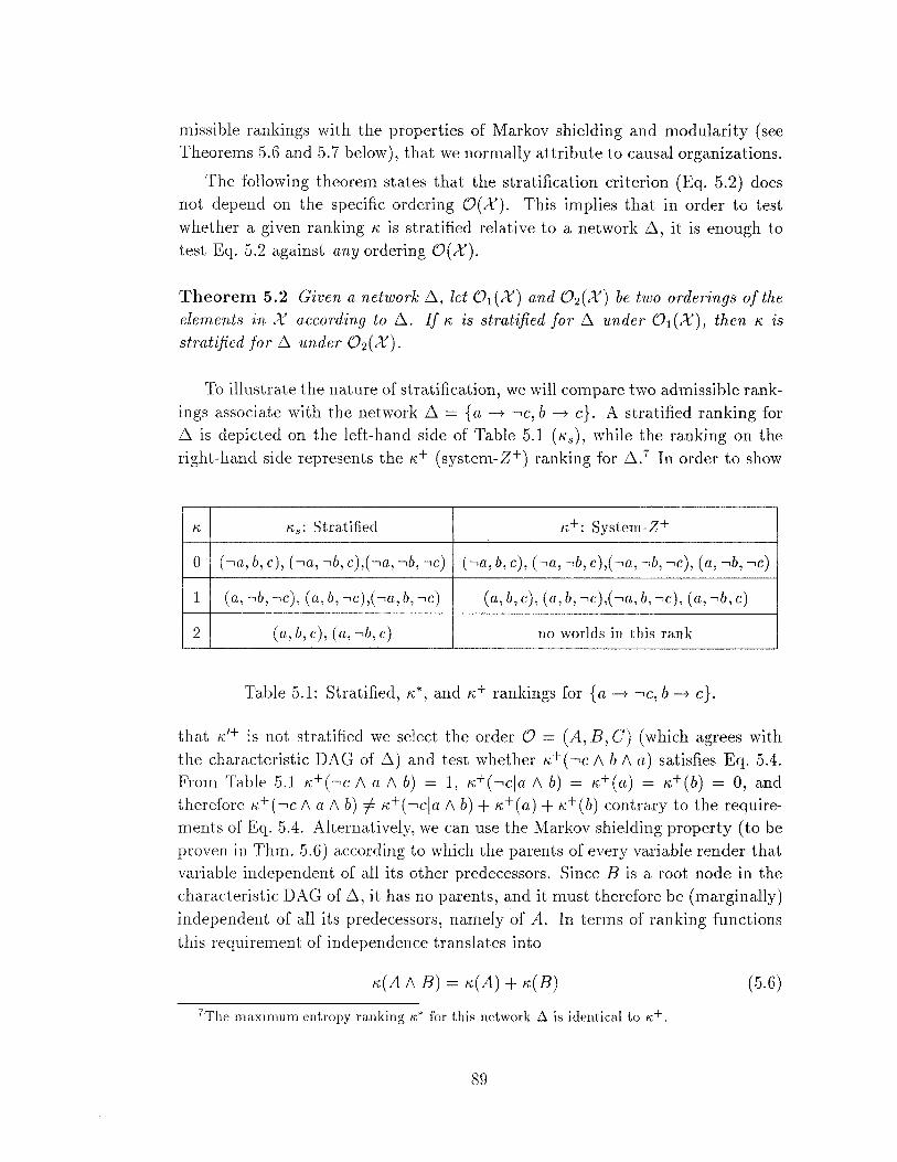
missible rankings with the properties of Markov shielding and modularity (see Theorems 5.6 and 5.7 below), that we normally attribute to causal organizations.

The following theorem states that the stratification criterion (Eq. 5.2) does not depend on the specific ordering O(X). This implies that in order to test whether a given ranking K is stratified relative to a network ~' it is enough to test Eq. 5.2 against any ordering O(X).

Theorem 5.2 Given a network~' let ('\(X) and 0 2(X) be two orderings of the elements in X according to ~. If K is stratified for ~ under 0 1 (X), then K is

stratified for~ under 02(X).

To illustrate the nature of stratification, we will compare two admissible rank­ings associate with the network ~ = {a --+ -.c, b --+ c}. A stratified ranking for ~ is depicted on the left-hand side of Table 5.1 (Ks), while the ranking on the right-hand side represents the K+ (system-Z+) ranking for ~. 7 In order to show

K Ks: Stratified K+: System-z+

0 (•a, b, c), (•a, •b, c),( •a, •b, •c) ( •a, b, c), ( •a, •b, c),( •a, •b, •c ), (a, •b, •c)

1 (a,•b,•c), (a,b,•c),(•a,b,•c) (a,b,c), (a,b,•c),(•a,b,•c), (a,•b,c)

2 (a, b, c), (a, •b, c) no worlds in this rank

Table 5.1: Stratified, K*, and K+ rankings for {a --+ -.c, b --+ c}.

that K1+ is not stratified we select the order 0 = (A, B, C) (which agrees with

the characteristic DAG of~) and test whether K+(-.c 1\ b 1\ a) satisfies Eq. 5.4. From Table 5.1 K+(-.c 1\ a 1\ b) = 1, K+(-.cja 1\ b) = K+(a) = K+(b) = 0, and therefore K+(-,c 1\ a 1\ b)-=/= K+(-.cja 1\ b)+ K+(a) + K+(b) contrary to the require­ments of Eq. 5.4. Alternatively, we can use the Markov shielding property (to be proven in Thm. 5.6) according to which the parents of every variable render that variable independent of all its other predecessors. Since B is a root node in the characteristic DAG of~' it has no parents, and it must therefore be (marginally) independent of all its predecessors, namely of A. In terms of ranking functions this requirement of independence translates into

K(A 1\ B)= K(A) + K(B) (5.6)

7The maximum entropy ranking K* for this network .6. is identical to K+.

89

for all instantiations of the literals A and B (taking values from {a, -.a} and {b, -.b} respectively). As can be verified from Table 5.1, I'Cs complies with Eq. 5.6.8

5.3 c-Entailment

Given a network 6 each stratified ranking "" defines a. consequence relation lk, II(

where ¢ I~ C5 iff ""( C5 1\ ¢) < K( •C5 1\ ¢) or if rc( ¢) = oo. A consequence relation is said to be proper for ¢ I~ C5 iff rc( ¢) -f oo.

Definition 5.3 ( c-Entailment) A network 6 c-entails C5 given¢, written¢ I~ C5,

iff¢ I~ C5 in every rc stratified for 6, which is proper for ¢I~ C5.

0

In other words, given 6, we can expect C5 from the evidence ¢, iff the preference constraint conveyed by ¢ -+ C5 is satisfied by every stratified ranking for 6. Def. 5.3 parallels the definition of f;- (probabilistic entailment, Def. 3.9) with the only difference being that the rankings for I~ must be stratified. We remark that c-entailment is not to be interpreted as stating that ¢ is believed to cause C5. Rather, it expresses an expectation to find C5 true in the context of ¢, having given a causal character to the rules in 6.

Since the set of stratified rankings for a given 6 is a subset of the admissible rankings for 6, every stratified consequence relation must satisfy the rules of inference of Logic) Cummulativity and Cases introduced in Section 3.2. It follows then, that the rules of inference below are sound for c-entailment.

Theorem 5.4 Let <.p, '1/J, ;, C5 1 and their conjunction be satisfiable wffs. The fol­lowing are sound rules of infe7'ence for 1~:

1. (Defaults) If <.p -+ '1/J (or <.p =} '1/J) E 6 then <.p I~ '1/J.

2. (Logic) If I= <.p :::> '1/J then <.p I~ '1/J.

3. (Augmentation) If <.pI~'!/' and <.pI~; then <.p 1\ ;I~ '1/J.

4. (Cut) If <.p /~;and <.p 1\ ;I~ '1/J then <.pI~ '1/J.

5. (Cases) If <.pI~ '1/J and;/~ '1/J then <.p V ;I~ '1/J.

The first rule (Default) follows immediately from the requirement of admissibility. Rules 2 and 5 correspond to the rules of Logic and Cases of Section 3.2, and rules 3

8 Eq. 5.6 can be also obtained from 5.5 by setting m = 2.

90

and 4 simple rewrite the Cum ulativity rule of Section 3. 2 by breaking the iff into two cases.

The following are derived rules of inference and further illustrate the logical properties of c-entailment and will be used in Examples. 5.1 and 5.2.9

Theorem 5.5 Derived rules of inference:

1. (Deductive closure) If 'P I~~ and 'P I~ 1 and I= 'P /\ ~ /\ 1 :) 0' then

'P I~ ()'

2. (Presuppositions) If 'P I~ ~ and 'P /\ 11~ ·~ then 'P I~ 'I·

3. (And) If 'PI~~ and 'PI~ 1 then 'PI~~/\ I·

These rules of inference are also sound with respect to p-entailment (and probabilistic entailment) and, therefore, as discussed in previous chapters, are too weak to constitute a full account of plausible reasoning. The next two the­orems provide additional inference power (reflecting the stratification condition) which emanates from the causal structure of 6. They establish conditions under which these inference rules can be applied modularly to subsets 6' C /::,.with the guarantee that the resulting inferences will hold in 6.

Theorem 5.6 Let /::,. be a network, and let {Pn ... , Ps} be a set of literals cor­

r·esponding to the parent set {xr, ... , xs} of Xt (each Pi, r :::; i :::; s, is either Xi

O'r •xi). Let ext denote a literal built on Xt, and let Y = {y1, ... , Ym} be a set

of atmnic propositions such that no Yi E y is a descendant of Xt in r (X,~). Let

c/Jy be any wff built only with elements from Y such that c/Jy /\ Pr /\ ... /\ Ps zs

satisfiable. rr p7' /\ ... /\ Ps I~ eXt then c/Jy /\ Pr /\ ... /\ Ps I~ eXt.

Theorem 5. 7 Let X' C X and !::,.' C /::,. such that all rules in !::,.' are built with

atomic pTopositions in X', and if x' E X' then all the rules in /::,. with either x'

OT as iheir consequent aTe also in 6'. Let 'P and ~ be two wffs built with

elements from X'. If 'P 1~, ~ then 'P I~ ~.

These theorems confirm that stratified rankings exhibit the properties of Markov shielding and modularity. As a corollary to Theorem 5. 7 it is easy to see that c-entailment is insensitive to irrelevant propositions, and moreover, given two net­works with no causal interaction, their respective sets of plausible conclusions will

9They are taken from [36] where a formal derivation in terms of the rules of inference in Theorem 5.4 can be found.

91

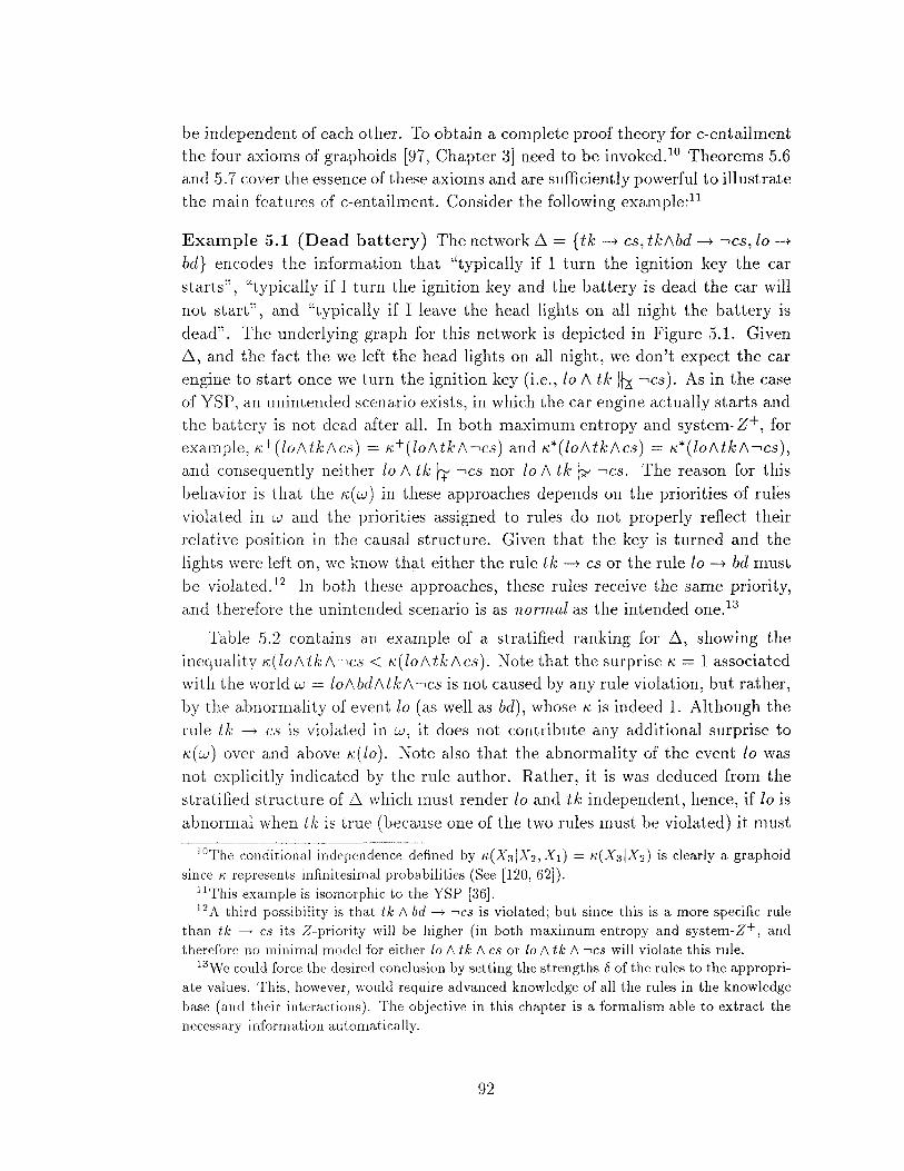
be independent of each other. To obtain a complete proof theory for c-entailment the four axioms of graphoids [97, Chapter 3] need to be invoked.10 Theorems 5.6 and 5.7 cover the essence of these axioms and are sufficiently powerful to illustrate the main features of c-entailment. Consider the following example:11

Example 5.1 (Dead battery) The network 6 = { tk-+ cs, tk/\bd-+ --,cs, lo-+ bd} encodes the information that "typically if I turn the ignition key the car starts", "typically if I turn the ignition key and the battery is dead the car will not start", and "typically if I leave the head lights on all night the battery is dead". The underlying graph for this network is depicted in Figure 5.1. Given 6, and the fact the we left the head lights on all night, we don't expect the car engine to start once we turn the ignition key (i.e., lo 1\ tk J~ -.cs ). As in the case of YSP, an unintended scenario exists, in which the car engine actually starts and the battery is not dead after all. In both maximum entropy and system-z+, for example, ,,+(Zo/\tk/\cs) = "'+(Zo/\tk/\--,cs) and ~>,*(lo/\tk/\cs) = ~>,*(lo/\tk/\--,cs),

and consequently neither lo 1\ tk f+ --,cs nor lo 1\ tk fy --,cs. The reason for this behavior is that the "'(w) in these approaches depends on the priorities of rules violated in w and the priorities assigned to rules do not properly reflect their relative position in the causal structure. Given that the key is turned and the lights were left on, we know that either the rule tk -+ cs or the rule lo -+ bd must be violated. 12 In both these approaches, these rules receive the same priority, and therefore the unintended scenario is as normal as the intended one. 13

Table 5.2 contains an example of a stratified ranking for 6, showing the inequality ~>,(lo/\tk/\--,cs < "'(lo/\tk/\cs). Note that the surprise"'= 1 associated with the world w lo/\bd/\tk/\--,cs is not caused by any rule violation, but rather, by the abnormality of event lo (as well as bd), whose "' is indeed 1. Although the rule tk -+ cs is violated in w, it does not contribute any additional surprise to "'(w) over and above "'(lo). Note also that the abnormality of the event lo was not explicitly indicated by the rule author. Rather, it is was deduced from the stratified structure of 6 which must render lo and tk independent, hence, if lois abnormal when tk is true (because one of the two rules must be violated) it must

10The conditional independence defined by tc(X3IX2, XI) = tc(X3IX2) is clearly a graphoid since K represents infinitesimal probabilities (See [120, 62]).

11 This example is isomorphic to the YSP [36]. 12 A third possibility is that tk 1\ bd -+ •cs is violated; but since this is a more specific rule

than tk -+ cs its Z-priority will be higher (in both maximum entropy and system-z+, and therefore no minimal model for either lo 1\ tk 1\ cs or lo 1\ tk 1\ •cs will violate this rule.

13We could force the desired conclusion by setting the strengths 8 of the rules to the appropri­ate values. This, however, would require advanced knowledge of all the rules in the knowledge base (and their interactions). The objective in this chapter is a formalism able to extract the necessary information automatically.

92

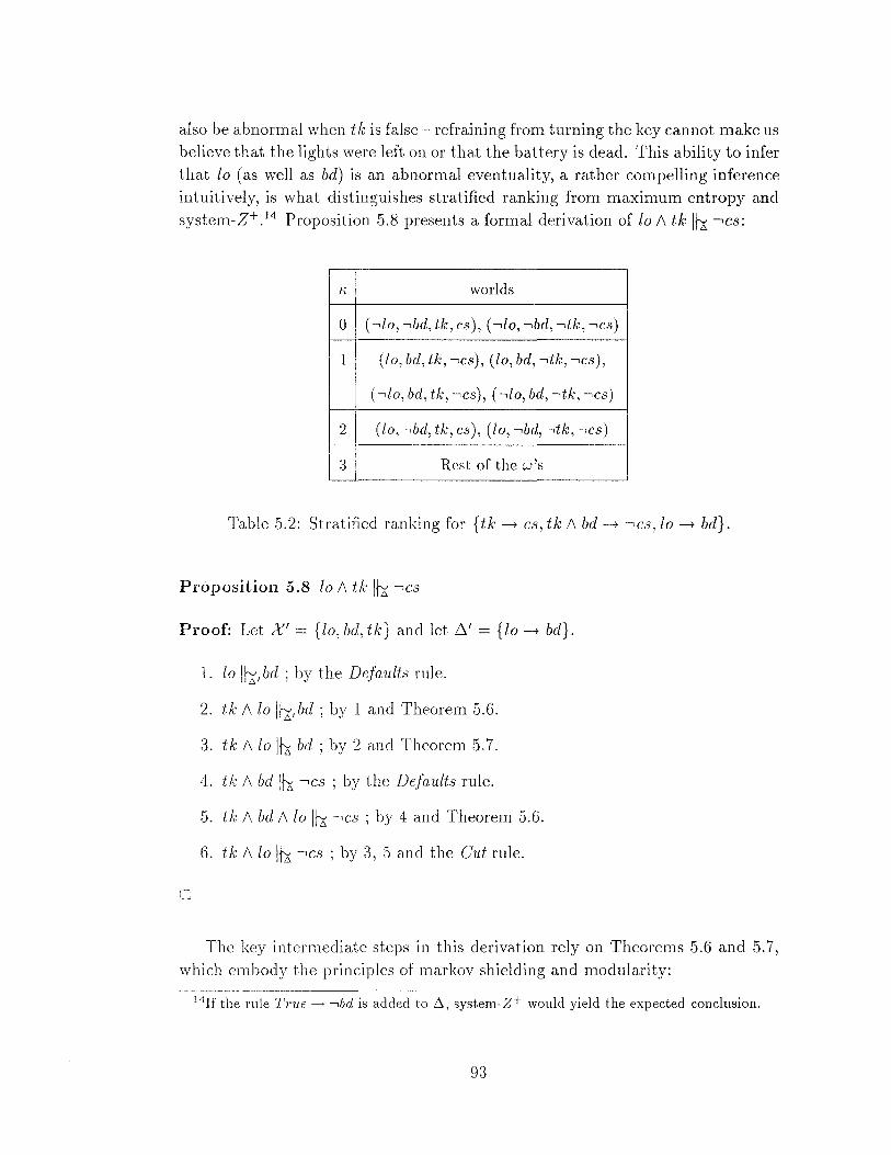
also be abnormal when tk is false- refraining from turning the key cannot make us believe that the lights were left on or that the battery is dead. This ability to infer that lo (as well as bd) is an abnormal eventuality, a rather compelling inference intuitively, is what distinguishes stratified ranking from maximum entropy and system-z+.14 Proposition 5.8 presents a formal derivation of lo 1\ tk I~ •cs:

/'i, worlds

0 ( -..lo, -..bd, tk, cs), (-.to, -..bd, -..tk, --,cs)

1 (lo, bd, tk, --,cs), (to, bd, -..tk, -..cs),

(-.to, bd, tk, -..cs), (-.to, bd, -..tk, -..cs)

2 (lo, -..bd, tk, cs), (lo, --,lJd, -..tk, -..cs)

3 Rest of thew's

Table 5.2: Stratified ranking for { tk ----t cs, tk 1\ bd ----t •c.s, lo----t bd}.

Proposition 5.8 lo 1\ tk I~ -.c.s

Proof: Let .-Y' {lo,bd,tk} and let!::.'= {lo----t bd}.

1. lo 1~,bd ; by the Defaults rule.

2. tk: 1\ lo I~, bd ; by 1 and Theorem 5.6.

3. tk 1\ lo I~ bd ; by 2 and Theorem 5.7.

4. tk 1\ bd I~ -.cs ; by the Defaults rule.

5. tk 1\ bd 1\ lo I~ •c.s ; by 4 and Theorem 5.6.

6. tk 1\ lo I~ •cs ; by 3, 5 and the Cut rule.

0

The key intermediate steps in this derivation rely on Theorems 5.6 and 5.7, which embody the principles of markov shielding and modularity:

14If the rule T1>ue-+ -..bd is added to .6., system-z+ would yield the expected conclusion.

93

• tk 1\ lo lh bd. This follows from the proposition tk and applying Theo­rem 5.7 to the sub-network D.' built from the language X'= { lo.bd.tk} and containing only the rule lo ---+ bd.

• tk 1\ bd !h •cs and tk 1\ bd 1\ lo lh •cs. The former follows directly from p­entailment, and the latter from applying Theorem 5.6 to the rule tk 1\ bd ---+

•cs, and the proposition lo.

The next example presents a simple abduction (or backward projection) prob­lem, and permits us to compare the behavior of c-entailment with that of chrono­logical minimization [118].

Example 5.2 (Unloading the gun.) Consider

standing for the various instances of "typically, if a gun is loaded at time ti, then

it is expected to remain loaded at time ti+l" (0 ::=:; i < n ). We say that a rule

li ---+ li+I is falsified by w iff w I= li 1\ -,[i+l; a stratified ranking K relative to D. can be constructed as follows:

K( w) = number of rules in D. falsified by w (5.7)

Given that the gun is loaded at t0 and that it is found unloaded at time

tn (i.e., l0 1\ •ln is true), the scheme of chronological minimization will favor the

somewhat counterintuitive inference that the gun remained loaded until tn-l (i.e.,

l1 1\ ... 1\ ln-l is true). c-entailment on the other hand, only yields the weaker

conclusion that the gun must have been unloaded any time within t1 and tn-l

(i.e., -.(h 1\ ... 1\ ln)), but the exact instant where the "unloading" of the gun occurs remains uncertain.

Proposition 5.9 lo 1\ •ln I~ •( l1 1\ ... 1\ ln)

Proof: Follows trivially from the Deduction rule. The fact that we cannot point

out the exact moment in which the gun is unloaded follows from the ranking built

by Eq. 5.7, since all formulas representing these situations have equal ranking. D

c-entailment and chronological minimization are expected to yield the same

conclusions in problems of pure prediction, since enforcing ignorance of future

events is paramount to the principle of modularity, which was shown to be inher­

ent to c-entailment. They differ however in tasks of abduction, as demonstrated

94

m Example 5.2. In this respect, c-entailment is closer to both motivated ac­tion theory [121] and causal entaament [36]. However, contrary to the motivated action theory, c-entailment automatically enforces specificity-based preferences, which are natural consequences of the conditional interpretation of rules. 15

Vve end this section by discussing the strict version of a causal rule denoted by =?, which will be useful in representing non-defeasible causal influences in Sections 5.3.2 and 5.4. Semantically, strict rules impose the following constraints on the admissibility conditions of a ranking K (Eq. 5.1): for each 1.p =? '1/J in the knowledge base,

K( 1/J 1\ i.p) < K( •1/J 1\ i.p) = oo, and K( i.p) < 00. (5.8)

Intuitively, a strict conditional voids interpretations that render its antecedent true and its consequent false by assigning them the lowest possible preference; a rank K equal to infinity.16 The following are two properties of strict rules:

Proposition 5.10 Let C1 1\ ... 1\ Cn =? E E 6

1. ( Contraposition) If there exists a stratified ranking for 6 where K( •E) < 00 then ·E I~ ·( cl 1\ ... 1\ Cn)

2. (Transitivity) If i.p I~ 1/J and 1/J /= (C1 1\ ... 1\ Cn) then i.p I~ E

These properties mirror the behavior of the material implication ":::)'', but the resemblance is in fact only superficiaL As discussed in Sections 2.1 and 2. 7, the

semantic difference between a strict rule c =? e and the wff c ::::> e is that the for­mer expresses necessary hence permanent constraints while the latter expresses information bound to the current situation. Thus, the former participates in constraining the admissible rankings while the latter is treated as an "observa­

tion" formula •c V e, and can affect conclusions only by entering the antecedents

of queries. This difference is greatly accentuated when strict conditionals are treated as causal rules, because stratified rankings are more sensitive to the rule

format. Indeed, contraposing the rule a =? b into •b =? •a changes the causal relationship between a and b and this change should reflect on the resulting rank. Compare, for example, 6 1 { c --+ •b, a =? b} and fl 2 = c --+ -.b, -.b =? •a. Any stratified ranking for 6 1 must render a and c totally independent of each other, as two unrelated causes of the variable B.

1.5We remark that the formalism in (121] deals with a much richer time ontology than the formalism presented here, and with a first-order language.

16This is equivalent to requiring that P(1fY/Y') = 1 and P(y::>) > 0 (see 2.2).

95

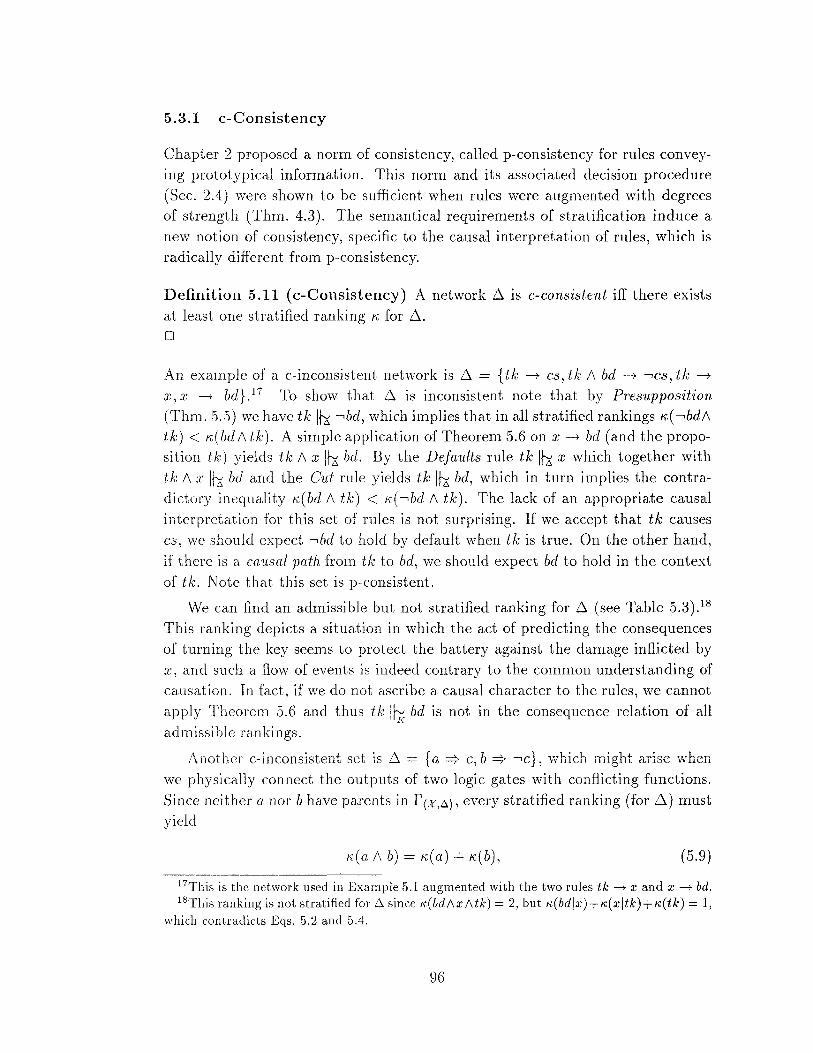
5.3.1 c-Consistency

Chapter 2 proposed a norm of consistency, called p-consistency for rules convey­ing prototypical information. This norm and its associated decision procedure (Sec. 2.4) were shown to be sufficient when rules were augmented with degrees of strength (Thm. 4.3). The semantical requirements of stratification induce a new notion of consistency, specific to the causal interpretation of rules, which is radically different from p-consistency.

Definition 5.11 ( c-Consistency) A network .6. is c-consistent iff there exists at least one stratified ranking 11, for .6.. 0

An example of a c-inconsistent network is 6 = { tk -+ cs, tl.: 1\ bd -+ --,cs, tk -+

x, x -+ bd} .17 To show that .6. is inconsistent note that by Presupposition (Thm. 5.5) we have tk lh: --,bd, which implies that in all stratified rankings 11,( --,bd/\ tk) < 11,(bd/\ tk). A simple application of Theorem 5.6 on x-+ bd (and the propo­sition tk) yields tk 1\ x lh: bd. By the Defaults rule tk !h: x which together with tk 1\ x lh: bd and the Cut rule yields tk !h; bd, which in turn implies the contra­dictory inequality 11,(bd 1\ tk) < 11,(--,bd 1\ tk). The lack of an appropriate causal interpretation for this set of rules is not surprising. If we accept that tk causes cs, we should expect --,bd to hold by default when tk is true. On the other hand, if there is a causal path from tk to bd, we should expect bd to hold in the context of tk. Note that this set is p-consistent.

We can find an admissible but not stratified ranking for .6. (see Table 5.3).18

This ranking depicts a situation in which the act of predicting the consequences of turning the key seems to protect the battery against the damage inflicted by x, and such a flow of events is indeed contrary to the common understanding of causation. In fact, if we do not ascribe a causal character to the rules, we cannot apply Theorem 5.6 and thus tk IL · bd is not in the consequence relation of all II(

admissible rankings.

Another c-inconsistent set is .6. = {a :::? c, b :::? --,c}, which might arise when we physically connect the outputs of two logic gates with conflicting functions.

Since neither a nor b have parents in f(x,,e..), every stratified ranking (for .6.) must yield

K(a 1\ b)= K(a) + K(b), (5.9)

17This is the network used in Example 5.1 augmented with the two rules tk-+ x and x -+ bd. 18This ranking is not stratified for 6.. since K(bd/\x/\tk) = 2, but K(bdlx)+K(xitk)+K(tk) = 1,

which contradicts Eqs. 5.2 and 5.4.

96

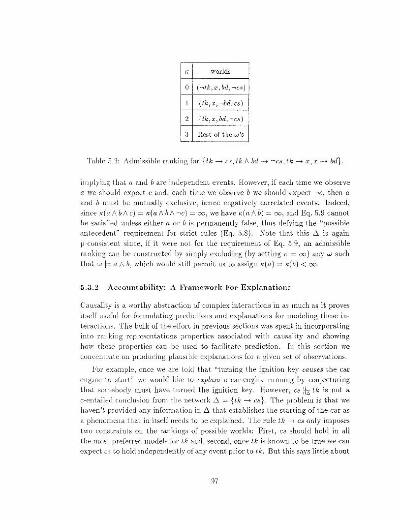
"" worlds

0 ( •ik, X, bd, •CS)

1 (tk, x, -.bd, cs)

2 (tk,x,bd,-.cs)

3 Rest of the w 's

Table 5.3: Admissible ranking for { tk--+ cs, tk 1\ bd--+ •cs, tk--+ x, x--+ bd}.

implying that a and bare independent events. However, if each time we observe a we should expect c and, each time we observe b we should expect •c, then a

and b must be mutually exclusive, hence negatively correlated events. Indeed,

since ""(al\bt~c) = K(al\bt~·c) = oo, we have K(al\b) = oo, and Eq. 5.9 cannot be satisfied unless either a or b is permanently false, thus defying the "possible antecedent" requirement for strict rules (Eq. 5.8). Note that this ~ is again p-consistent since, if it were not for the requirement of Eq. 5.9, an admissible

ranking can be constructed by simply excluding (by setting K = oo) any w such

that w I= a 1\ b, which would still permit us to assign K( a) = K( b) < oo.

5.3.2 Accountability: A Framework For Explanations

Causality is a worthy abstraction of complex interactions in as much as it proves

itself useful for formulating predictions and explanations for modeling these in­teractions. The bulk of the effort in previous sections was spent in incorporating into ranking representations properties associated with causality and showing how these properties can be used to facilitate prediction. In this section we concentrate on producing plausible explanations for a given set of observations.

For example, once we are told that "turning the ignition key causes the car

engine to start" we would like to explain a car-engine running by conjecturing

that somebody must have turned the ignition key. However, cs lf-x tk is not a c-entailed conclusion from the network ~ = { tk --+ cs}. The problem is that we haven't provided any information in ~ that establishes the starting of the car as

a phenomena that in itself needs to be explained. The rule tk --+ cs only imposes two constraints on the rankings of possible worlds: First, c.s should hold in all the most preferred models for tk and, second, once tk is known to be true we can expect c.s to hold independently of any event prior to tk. But this says little about

97

the models of •cs and, in particular, whether the car will start without turning the ignition key. In normal discourse, when given a set of rules "Ci causes E" we

usually subscribe (by convention) to additional assumptions that help complete this information. 19 Three of the most common assumptions are:

• Accountability: An effect E is presumed false if all the conditions listed as causes of E are also false. 20

• Exception Independence: The rules representing the "cause-effect" re­lations may admit exceptions which inhibit the occurrence of the effect even in prescence of the cause. However, unless explicitly stated or logically im­plied, these exceptions are presumed independent. In the car example, a.

dead-battery and an empty gas tank can be considered as such exceptions to tk ---t cs. Both will prevent the car engine from starting, and are presumed to be independent of each other.

• Disjunctive Interaction: The likelihood of an event does not diminish when several of its causes prevail simultaneously. For example, if rain and sprinkler-on are each a cause for the grass being wet, the grass will be only more likely to be wet if both the sprinkler is turned on and it is raining. 21

A probabilistic model that captures these assumptions, called noisy-or gate, is described in [97] where it is proposed as a canonical model of disjunctive interac­tion among causes C1 , ... , Cn that predict the same effect E. The noisy-or gate is depicted schematically in Fig. 5.3. The set {I1 , ..• , In} represents inhibitors, where each Ii stands for an abnormality that would interfere with the causal

connection between Ci and E. Every pair C; and I; constitutes the inputs to an

and-gate so that if Ci is "active" (or true) and Ii is not known to be active, then the output -"i will provide support for the effect E. Each Si is then an input to the final or-gate. If one or more of these s; 's is active then E is expected to be true, and if all s; are false, then E is expected to be false.

Both and-gates and or-gates impose functional constraints on propositions; thus, in order to represent their behavior strict rules are necessary. The rules in Eqs. 5.10~5.13 formalize the intended behavior of an and-gate:

ci A ·Ii =;. si (5.10)

19See [68] for a discussion on the relation between completing the information and abduction reasoning for tasks of producing explanations from observations.

20This may require that we lump together all unknown causes of E under the heading "all other causes".

21 This assumption actually follows from that of exception independence.

98

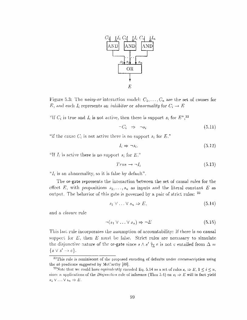
t E

Figure 5.3: The noisy-or interaction model: C1 , ... , Cn are the set of causes for E, and each 1; represents an inhibitor or abnormality for C; -+ E

"If C; is true and 1; is not active, then there is support s; for E" ,22

( 5.11)

"if the cause C; is not active there is no support s; for E."

(5.12)

"If 1; is active there is no support s; for E."

(5.13)

"I; is an a.bnormality, so it is false by default".

The or-gate represents the interaction between the set of causal rules for the effect E, with propositions 8 1 , ... , 8n as inputs and the literal constant E as output. The behavior of this gate is governed by a pair of strict rules: 23

81 V ... V 8n :::} E, (5.14)

and a closuTe rule

(5.15)

This last rule incorporates the assumption of accountability: If there is no causal support for E, then E must be false. Strict rules are necessary to simulate the disjunctive nature of the or-gate since 8 1\ 8

1 I~ e is not c-entailed from 6 =

{ 8 V 81 -+ e }.

22This rule is reminiscent of the proposed encoding of defaults under circumscription using the ab predicate suggested by McCarthy [88].

23Note that we could have equivalently encoded Eq. 5.14 as a set of rules Si =? E, 1 :::; i :::; n, since n applications of the Disjmtction rule of inference (Thm 5.4) on si =? E will in fact yield s1 V ... V Sn =? E.

99

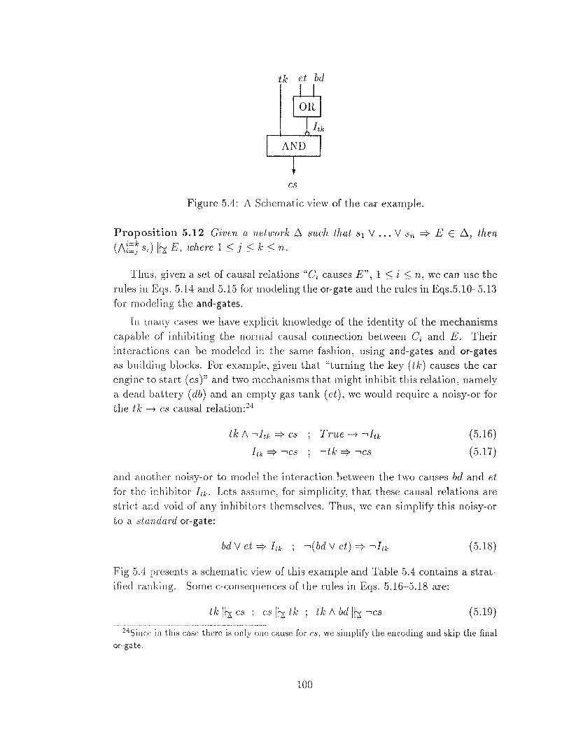
tk et bd

cs

Figure 5.4: A Schematic view of the car example.

Proposition 5.12 Given a network 6 such that s1 V ... V sn =? E E 6, then

(1\~=:,J si) ItA E, where 1 :S; j :::; k :::; n.

Thus, given a set of causal relations "Ci causes E", 1 :::; i :::; n, we can use the rules in Eqs. 5.14 and 5.15 for modeling the or-gate and the rules in Eqs.5.10-5.13 for modeling the and-gates.

In rnany cases we have explicit knowledge of the identity of the mechanisms capable of inhibiting the norma.l causal connection between Ci and E. Their interactions can be modeled in the same fashion, using and-gates and or-gates as building blocks. For example, given that "turning the key ( tk) causes the car engine to start ( cs )" and two mechanisms that might inhibit this relation, namely a dead battery (db) and an empty gas tank (et), we would require a noisy-or for the tk ---+ cs causal relation: 24

True ---+ •ltk

•tk =} •CS

(5.16)

(5.17)

and another noisy-or to model the interaction between the two causes bd and et

for the inhibitor Itk· Lets assume, for simplicity, that these causa.l relations are strict and void of any inhibitors themselves. Thus, we can simplify this noisy-or to a standard or-gate:

bd V et =? Itk ; •( bd V et) =? •ltk (5.18)

Fig 5.4 presents a schematic view of this example and Table 5.4 contains a strat­ified ranking. Some c-consequences of the rules in Eqs. 5.16-5.18 are:

tk ItA cs ; cs ItA tk ; tk 1\ bd ItA -.cs (5.19)

24 Since in this case there is only one cause for cs, we simplify the encoding and skip the final or-gate.

100

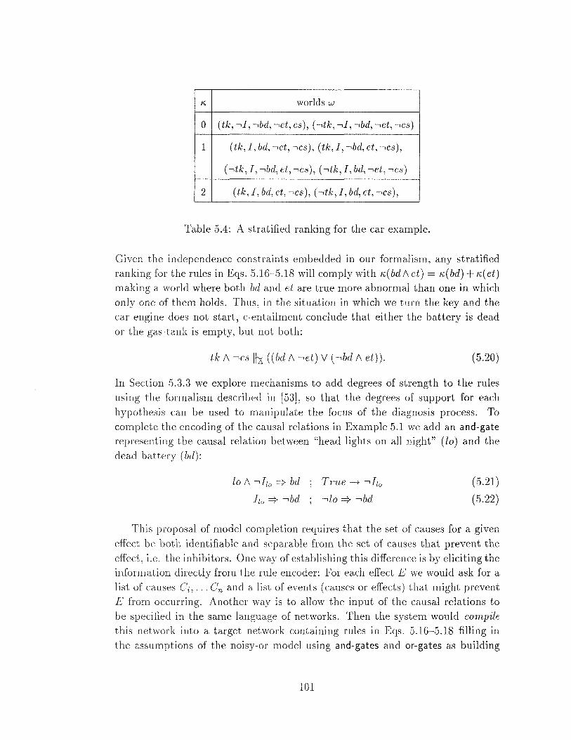
K, worlds w

0 ( tk, ·I, ·bd, •et, cs), ( •tk, -,I, -,bd, •et, •cs)

1 (tk, I, bd, •et, •cs), (tk, I, ·bd, et, •cs),

(•tk,I,·bd,et,•cs), (•tk,I,bd,-,et,•cs)

2 (tk,I,bd,et,•cs), (•tk,I,bd,et,•cs),

Table 5.4: A stratified ranking for the car example.

Given the independence constraints embedded in our formalism, any stratified ranking for the rules in Eqs. 5.16-5.18 will comply with "'(bd 1\ et) = "'( bd) + "'( et) making a world where both bd and et are true more abnormal than one in which only one of them holds. Thus, in the situation in which we turn the key and the car engine does not start, c-entailment conclude that either the battery is dead or the gas-tank is empty, but not both:

tk 1\ -.cs I~ ((bd 1\ -.et) V (-.bd 1\ et)). (5.20)

In Section 5.3.3 we explore mechanisms to add degrees of strength to the rules using the forma.lism described in [53], so that the degrees of support for each hypothesis can be used to manipulate the focus of the diagnosis process. To complete the encoding of the causal relations in Example 5.1 we add an and-gate representing the causal relation between "head lights on all night" ( lo) and the dead battery (bd):

lo 1\ -.flo :::} bd

Ito =? -.bd

(5.21)

(5.22)

This proposal of model completion requires that the set of causes for a given effect be both identifiable and separable from the set of causes that prevent the effect, i.e. the inhibitors. One way of establishing this difference is by eliciting the information directly from the rule encoder: For each effect E we would ask for a list of causes Ci, ... Cn and a list of events (causes or effects) that might prevent E from occurring. Another way is to allow the input of the causal relations to be speci{~ed in the same language of networks. Then the system would compile this network into a target network containing rules in Eqs. 5.16-5.18 filling in the assumptions of the noisy-or model using and-gates and or-gates as building

101

blocks. This process would examine the rules family by family25 following the stratified order imposed by the underlying graph of 6. In case of conflicting

relations, i.e. a set of literal supporting an effect e and another set supporting •e, the system will try to uncover the inhibitor from the causes by using the rule of Presupposition in Theorem 5.5. This rule of inference says that if C; I~ E and C; 1\ I; I~ •E then Ci I~ •h Thus, in the car example we would have the set 6 = { tk -+ cs, bd 1\ tk =} •cs, et 1\ tk =} •cs} as input, and a simple application of the rule of Presupposition will mark both bd and et as inhibitors with respect to tk. Note that cases of ambiguous families like {a -+ c, b -+ •c} would require further information about the relation between a and b, since first we cannot distinguish between causes and inhibitors, and second, an encoding of both these rules as and-gates will result in a c-inconsistent network similar to the example of conflicting strict arrows in Section 5.3.1. The problem is tha.t the assumption of exception independence is no longer valid: The cause for c (i.e., a) is the inhibitor for the cause of •c (i.e., b) and vice-versa.

5.3.3 The most normal stratified ranking

In Section 5.3.2 we saw that in order to reap the full benefits of Bayesian Net­works, we needed to supplement the constraints of 6 with additional informa­tion that further shapes the conditional rankings of each famjly in the underlying DAG. Another approach of supplementing the missing information is to establish a preference relation among stratified rankings and rule out those rankings that are less preferred than others. Since a lower ranking is associated with greater normality, it is natural that out of the set of all admissible stratified rankings we prefer those that assign to interpretations the lowest possible ranks, and then define the entailment relation with respect to this set of privileged rankings.

Such a strategy was adopted in Chapter 4 (without the requirement of strat­ification) and led to system-z+. The incorporation of the most-normal strategy in the context of stratified rankings, will result in a substantial increase of ex­pressiveness. For example, in the noisy-or encoding of causal relations, assuming independence among the inhibitors, the most-normal (minima.l) stratified ranking 11:t is given by the following function:

11:t ( w) = number of inhibitors that are true in w (5.23)

Thus, in the car example (with dead battery and empty tank as inhibitors) in Eqs .. 5.16~5.18, the minimal ranking Kt(w) will be 0, 1 or 2 depending on whether

25 A family is the set of propositions corn posed by the parent set of an effect and the effect itself (Section 5.2).

102

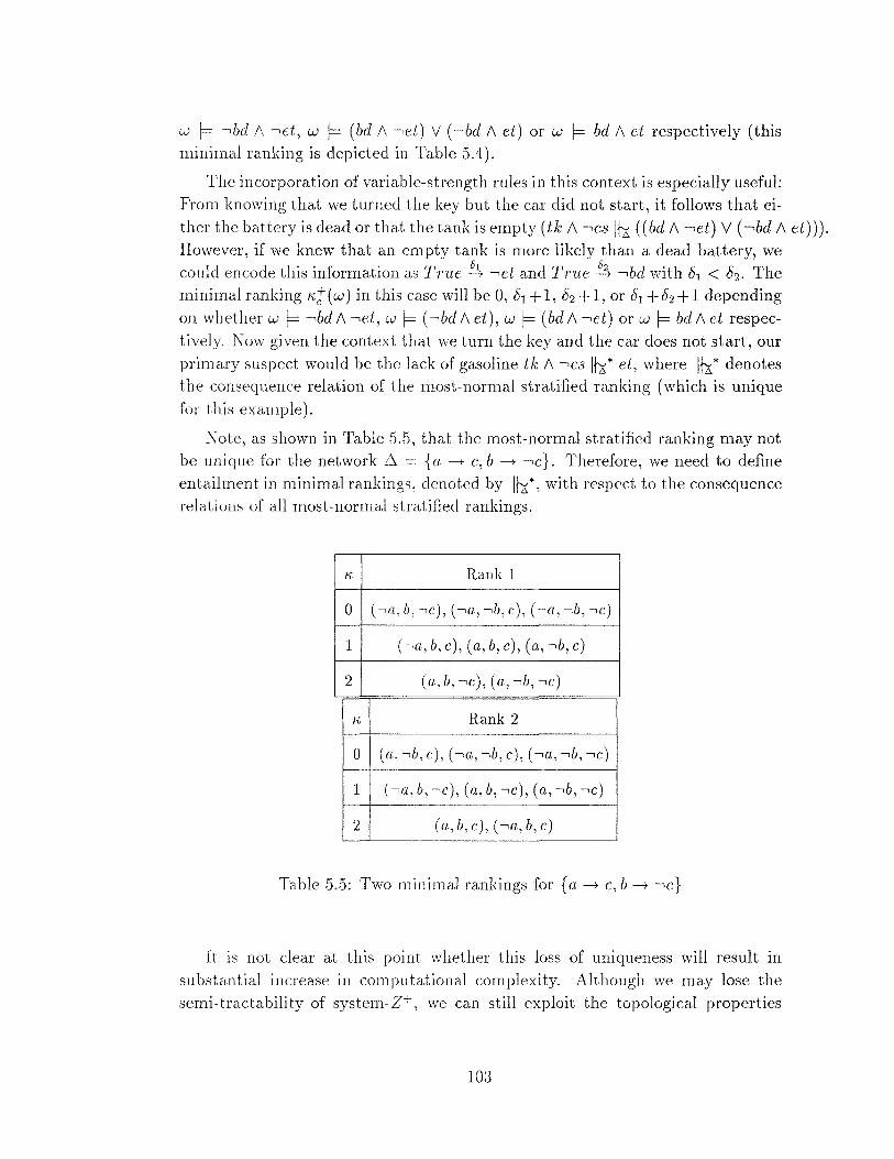
w f= ·bd 1\ •et, w f= (bd 1\ •et) V (•bd 1\ et) or w f= bd 1\ et respectively (this minimal ranking is depicted in Table 5.4).

The incorporation of varia.ble-strength rules in this context is especially useful: From knowing that we turned the key but the car did not start, it follows that ei-

ther the battery is dead or that the tank is empty ( tk 1\ •cs I~ ( ( bd 1\ •et) V (-,bel 1\ et))). However, if we knew that an empty tank is more likely than a dead battery, we could encode this information as True ~ -,et and True ~ ·bel with 81 < 82• The minimal ranking Kt ( w) in this case will be 0, 81 + 1, 82 + 1, or 81 + 82 + 1 depending

on whether w f= ·bd 1\ •et, w f= ( ·bd 1\ et), w f= (bel 1\ •ei) or w f= bd 1\ et respec­tively. Now given the context that we turn the key and the car does not start, our primary suspect would be the lack of gasoline tk 1\ •cs I~* et, where I~* denotes the consequence relation of the most-norma.l stratified ranking (which is unique

for this example).

Note, as shown in Table 5.5, that the most-normal stratified ranking may not be unique for the network 6 = {a -+ c, b -+ •c}. Therefore, we need to define entailment in minimal rankings, denoted by I~*, with respect to the consequence relations of all most-norma.l stratified rankings.

K Rank 1

0 (-,a, b, -,c), (-,a, -,b, c), (-,a, -,b, -,c)

1 (-,a, b, c), (a, b, c), (a, -,b, c)

2 (a, b, -,c), (a, -,b, -,c)

K Rank 2

0 (a,-,b,c), (-,a,-,b,c), (....,a,-,b,-,c)

1 (-,a,b,-,c), (a,b,-,c), (a,-,b,-,c)

2 (a,b,c), (-,a,b,c)

Table 5.5: Two minimal rankings for {a -+ c, b -+ •c}

It is not clear at this point whether this loss of uniqueness will result in substantial increase in computationa.l complexity. Although we may lose the serni- tractability of system-z+, we can still exploit the topological properties

103

of the characteristic DAG (f(X,L}.)) to render practical reasoning feasible. It is well known that the local propagation techniques of Bayesian Networks can be extended to sparse networks by embedding the network in a hypertree (or acyclic database) [115]. Thus, it is quite feasible that similar techniques could be applied to the computation of consequences in systems governed by the "most-normal" completion of stratified rankings.

5.4 Belief Update

Section 4.6 demonstrated how the semantics of model ranking, together with the syntactic machinery developed for system-z+, can be applied to manage the tasks of belief revision, in conformity with the AGM postulates. The introduction of stratified ranking adds the capability for implementing a new type of belief changes, named update by Katsuno and Mendelzon (KM) [65]. In both tasks (be­lief revision and belief update) we seek to incorporate a new piece of information rP into an existing set of beliefs ~'· Yet, in belief revision rjJ is assumed to be a piece of evidence while in update rjJ is treated as a change occurring by external intervention. Katsuno and Mendelzon (65] have shown that the AGM postulates are inadequate for describing changes caused by updates, for which they have proposed new sets of postulates. The basic difference between revision and up­date is that the latter permits changes in each possible world independently, as was proposed by Winslett [127]. 26

Belief update can be embodied in a stratified ranking system using the fol­lowing device: For each instruction to "update the knowledge base by rjl" we add a set of rules that simulates the action "do( rjJ ), leaving everything else constant (whenever possible)", and then condition K on the truth of do( rjJ). The following set of causal rules embody the intent of this action, where rjJ and r/J' stand for "r/J holds at t" and "r/J holds at t' > t", respectively: 27

rP --7 r/J'

'rP --7 ·¢' do( rP) => r/l'.

(5.24)

(5.25)

(5.26)

The following example (adapted from Winslett [127]) demonstrates how this de­vice differentiates between update and revision.

26 In the language of Bayesian networks, the difference between updates and revisions parallels the distinction between causal and evidential information [96].

27The two persistence rules, Eqs. 5.24 and 5.25, are presumed to apply between any two atomic propositions at two successive times.

104

Example 5.3 (XOR-gate) A XOR Boolean gate c =X OR( a, b) is examined at two different times. At time t, we observe the output c = true and conclude that one of the inputs a or b must be true, but not both. At a later time t' we learn that b' is true (primed letters denote propositions at timet'), and we wish to change our beliefs (in a and a') accordingly. Naturally, this change should depend on how the truth of b' is learned. If we learn b' by measuring the voltage on the b terminal of the gate, then we have a belief revision process on our hands, and we expect a' to be false. On the other hand, if we learn that b' is true as a result of physically connecting the b terminal to a voltage source, we no longer expect a' to be false, since we have no reason to believe that the output c has retained its truth value in the process.

In tbe stratified ranking forrnula.tion, the knowledge base corresponding to this example will consist of three components:

1. The functional description of the XOR gate at times t and t',

a 1\ b ::::} -,c

a 1\ -, b ::::} c

and a.n equivalent set of rules for a', b', c'.

2. The persistence rules: For every x in {a, b, c},

:r -+ x' ; -,x -+ -,x'.

3. The action do(b), which represents the external influence on b':

do( b) ::::} b'.

(5.27)

(5.28)

(5.29)

(5.30)

The underlying graph for the network 6 corresponding to this knowledge base is depicted in Figure 5.5.

Initially, after observing c, our evidence consists only of c. The minimal stratified ranking K-c for a 6 consisting of rules in Eqs. 5.27-:5.30 is depicted in Table 5.6. To represent belief revision, we add b' to our evidence set and query whether c 1\ b' ff'x* -,a'. 28 In contrast, to represent belief update, we add do(b) to our evidence set and query whether ( c 1\ b' 1\ do( b)) ff'x* -,a'.

It is easy to show that the first query is answered in the affirmative, while the second in the negative. The left-hand side of Table 5. 7 shows the ranking

28 Recall that II-A* denotes the consequence relation of the minimal stratified ranking for 6. (see Sec. 5.3.3), which is unique for this example.

105

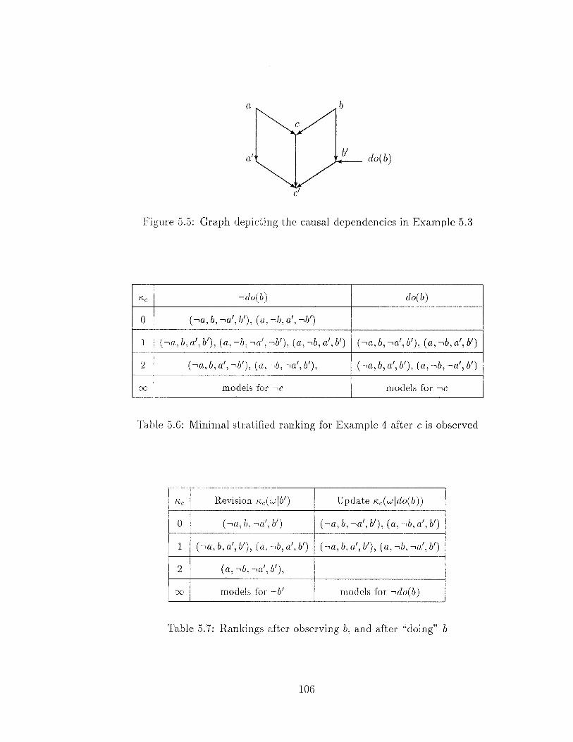
a b

a' b' .......-- do(b)

Figure 5.5: Graph depicting the causal dependencies in Example 5.3

K,c ·do(b) do( b)

0 (•a,b,•a',b'), (a,•b,a',•b')

1 (•a,b,a',b'), (a,•b,•a',---,f/), (a,•b,a',b') ( •a, b, •a', b'), (a, ---,b, a', b')

2 ( •a, b, a', •b'), (a, •b, •a', b'), ( •a, b, a', b'), (a, ---,b, •a', b')

00 models for •C models for •C

Table 5.6: Minimal stratified ranking for Example 4 after c is observed

K, c Revision ""c(wlb') Update ""c(wldo( b))

0 ( •a, b, •a', b') (•a,b,•a',b'), (a,•b,a',b')

1 ( •a, b, a', b'), (a, ---,b, a', l/) (•a,b,a',b'), (a,•b,•a',b')

2 (a, •b, •a', b'),

00 models for ·b' models for ·do(b)

Table 5. 7: Rankings after observing b, and after "doing" b

106

resulting from revising the ranking in Table 5.6 by b' (first query), while the right-hand side shows the ranking after updating by do(b) (second query). Note that in the revised ranking the only world in the zero rank is a model for ---.a', while the updated ranking shows an additional world which is a model for a'

(the state of the output c in this world changed as a consequence of the action). The action do(b) establishes the truth of b' but has no effect on what we believe about the second input a'. Since neither a nor ---.a were believed at t, they remain unbelieved at t'.

5.4.1 The dynamics of belief update

The example above demonstrates that, given a ranking 1\, and a network ~' it is possible to predict how a system would respond to external interventions. For example, if we wish to inquire whether event e will hold true after we force some variable A to become true, we simply add to ~ the rule do( a) ::::} a, 29 recompute the resulting stratified ranking r/ on the augmented set of variables (including do(a)), and then compute K, 1(eJdo(a)). There is a simple relation between K,(eJa) and n:'(eJdo(a)), which results in a direct transformation between two ranking

functions, K,(w) and K,do(a)(w), the latter being an abbreviation of K, 1(wJdo(a)). From Eq. 5.4 we have that:

t=n

~~(Xn 1\ ... 1\ A 1\ ... 1\ )(I) L 1\,(XnJParxn) (5.31) i=l

K,(Xn 1\ ... I\ A 1\ ... 1\ X1) = L 1\,(XnJParx,J + K,(AJParA) (S.32) i=l,i:;i:j

where A is the jlh literal taking values from {a, ---.a}. Similarly, the stratification of K, 1 relative to ~ U {do( a) ::::} a} dictates

K, 1(Xn 1\, .. I\ A 1\ ... I\ X1 1\ DO(a)) = t=n

L K,'(XnlParxJ + t~'(AJPar~) + K, 1(DO(a)) (S.33) i=l,i:;i:j

29 Vle use lowercase to denote the instantiation of variable A to a truth value.

107

Where DO(a) is a variable taking values from {do(a),•do(a)}, Par~= ParA U {Do(a)}, and

0 if A= a and DO(a) = do(a),

n:'(A\Par~) = n:(A\ParA) if DO(a) = do(a), (5.34)

00 • C A ·~ 1 no( \ 1 ( \ 11 .li = •a ana v a) = ao a).

Eq. 5.33 reflects the fact that the action variable DO( a) is a root node in r (X,-6.),

since it is under the sole contml of the rule author, while Eq. 5.34 reflects the constraint do( a) ::;. a. Since the new rule do( a) ::;. a only affects the family of A, we have that the summation term in Eq. 5.33 is equal to the summation term in Eq. 5.32. Conditioning Eq. 5.33 on do( a) and making the appropriate substitutions yields

n:'(Xn 1\ ... 1\ A 1\ ... 1\ X1\do(a)) = n:(Xn 1\ ... 1\ A 1\ ... 1\ X1)­

-n:(A\ParA) + n:'(A\ParA 1\ do( a)) (5.35)

Where, according to Eq. 5.311, r.:'(A\Pm'AI\do(a)) = 0 when A= a, and n:'(A\ParAI\ do( a)) = oo when A = •a. Thus, making again the appropriate substitutions we get

{

n:(w)- n:(a\ParA(w)) if w \=a. A:do(a)(w) =

oo if w •a.

(5.36)

In other words, the n: of each world w satisfying a is reduced by an amount equal to the degree of surprise of finding A true, given the realization of Par A in w (denoted by Pm'A(w). The 1;; of each world falsifying a is of course oo.30

Such independent movement from world to world is shown in Example 5.3, where n:(w) is depicted on the left-hand side of Table 5.6 and n:da(w) is depicted on the right hand side of Table 5.7. If A has no parents (direct causes), then A:do(a) is obtained by shifting the n: of each w I= a by a constant amount n:( a), as in ordinary conditioning, and n:do(a)(w) would be equal to n:(w\a), as expected. However, when the manipulated variable has direct causes ParA, the amount of

30The reader might recognize Eq. 5.36 in its probabilistic form where, given a probability function P(w) and a causal network r, the probability P'(w) obtained by manipulating variable A to take on the value a is given by: P'(w) = P(w)/ P(aiPm·A(w)) (for w I= a). This can be easily shown from the functional definition of causal relationships as used, for example, in Pearl and Verma [103].

108

shift would vary from world to world, depending on how surprising it would be

(in that world) to find a happening naturally (without external intervention). For instance, if A is governed by persistence rules, a( t -1) -t a( t), •a( t -1) -t ..,a( t), then worlds in which a( t - 1) hold will shift less than those in which a( t 1) is false, because a(t) is expected to hold in the former and not in the latter. Note that the amount of shift subtracted from A:( w) is equal precisely to the fraction of surprise A:(aiPaiA(w)) that A i1ue contributes to A:(w) and that now becomes explained away (hence excusable) by the action do(a). The generalization of Eq. 5.36 to the case where a conjunction of literals <P = a1 1\ •a2 ..• are forced to become true or false is straightforward:

(5.37)

if w I= </J, and li:do(¢)(w) = oo otherwise.

Note that any stratified ranking n; has at least one variable A possessing a remarkable invariant properties:

c { A:(w) li:do(a)(w) =

00

if w I= a, (5.38)

otherwise.

Intuitively, every variable satisfying Eq. 5.38 corresponds to a sink in f (X,A}, or a "last" variable in the "tempora.l" ordering 0. Indeed, for any such sink, Eq. 5.38 conveys the intuition that by manipulating the last variable in the temporal order, we do not expect the past to change. It is comforting to see that the ramifications of the Markov shielding principle coincide with an alternate reading of causation

as a specification of behavior under external interventions.

5.4.2 Relation to KM postulates

Katsuno and Mendelzon [65] have formulated belief update as a transformation between two formulas, 7/J, representing our current set of beliefs, and </J, the new information we wish to incorporate into that set of beliefs. The update process is assumed to be an operator o that takes the formula 7/J and transforms it into a new formula 7/J o </J, that syntactica.lly represents our updated set of beliefs. KM have introduced a set of postulates which characterize all update operators that can be defined by the possible world approach of Winslett [127], hence, they are considered universal conditions for any model describing belief change due to external actions. One such postulate, for example,

(U2) If 7/J implies </J, then 7/J o <Pis equivalent to 7/J,

109

says that if the new sentence¢ is derivable from belief set 7/J, that updating by¢ does not alter the belief set.

In our ranked-based model of beliefs change, the current stock of beliefs is represented by those worlds w for which rv is zero. Hence, 1p is defined by the union of all w such that k( w) = 0. If the new sentence ( ¢) is a conjunction of literals, then the updated ranking is given by Eq 5.37 and the new set of beliefs, 7/J o ¢,is represented semantically by the union of all worlds w for which rvdo(¢)( w) is zero.31

That updates resulting from Eq. 5.36 comply with the KM postulates can be seen by the following consideration. KM have shown that their axioms are equivalent to the existence of a function mapping each possible interpretation world w to a partial pre-order ::::;w, such that for any interpretation w', if w =f. w'

then w <w d. Then the set of models for the update of a fonnula 7/J (representing our current beliefs) by a formula ¢, written 7/J <> ¢, is found by taking the union of the minimal models for ¢, with respect to each one of the pre-orders defined by the models for 7/J:

Mods ( 7/J <> ¢) = u min(111ods(¢), ::::;w)· (5.39) wEMods(,P)

In other words, Eq. 5.39 asserts that the models of 'IP <> ¢ can be obtained by replacing each 7/J-world w with a set of ¢-worlds w* that are nea·rest to w. We shall call each such w* an image of w, a word coined by Lewis [77] to denote a counterfactual alternative to Bayes conditioning. If w is consistent with ¢ then its image w* is equal to w itself, as is required by ::::;w. However, when w is inconsistent with ¢, its iinage is a closest (according to ::::;w) world satisfying ¢.

Thus, to show compliance with the KM postulates we need to define a preorder ::::;w a.nd show that for every world w •¢ that is currently assigned rv(w) = 0, Eq. 5.37 takes each image w* of w and moves it toward KJo(¢)(w*) = 0. We shall construct such a preorder and show that, moreover, in an in1age world w*, every

31 Updates involving disjunctions require special treatment. If they are to be interpreted as a license to effect any change satisfying the disjunction, then the final state of belief is the union, taken over all disjuncts, of worlds that drift to K = 0. In this interpretation, the instruction ''make sure the box is painted either blue or white" will leave the box color unknown, even knowing that the box was white initially (contrary to the postulate (U2) of KM). However, if the intention is to effect no change as long as the disjunctive condition is satisfied, then the knowledge base should be augmented with an observation-dependent strategy "do( cp) when cp is not satisfied", instead of using the pure action do( cp ). Conditioning on such a strategy again yields a belief set consistent with the KM postulates. The first interpretation is useful for discrediting earlier observations, for example, "I am not sure the employee's sa.lary is 50!(; it could be anywhere between 40!{ and 60K".

110

term A:(x;!Pm'xJw*)) > 0 represents a violation of expectation that would be totally excusable were it caused by an external intervention such as ¢. Intuitively, the image world corresponds to a scenario in which all the unexpected events are attributed to the intervention of ¢ but otherwise the world follows its natural, unperturbed course as dictated by the prediction of the causa.l theory.

It is not hard to see that the image w* as described above is indeed a minimal element in the order :Sw, defined as follows:

Definition 5.13 (World orderings) Let 0 = x 1 ,x2 , ... ,xn be any order of the variables that is consistent with the DAG f(x,D.)· Given three worlds w,w1 ,

and w 2 , we say that w1 :Sw w2 iff the following conditions hold:

0

1. w disagrees with w2 on a literal that is earlier (in 0) than any literal on which w disagrees with w1 .

Theorem 5.14 Let '1/J be a w.ff repr-esenting a set of beliefs. Let 11: be a r-anking

such that w E Aiods('l/J) iff 11:(w) = 0. Let¢ repTesent a conjunction of literals,

and let "'do(<P) be the mnking that results f1'0m updating"' by¢ as shown in Eq. 5.36

such thalw* E 111ods('l/Jo¢) i./JA:do(¢)(w*) = 0. Then

111 ods( '1/J o ¢) = u min(l\1ods(¢), :Sw)· (5.40) wEMods(.,P)

5.4.3 Related work

The connection between belief update and theories of action was noted by Winslett in [127] and has been elaborated more recently by del Val and Shoham [22] using the situation calculus. In fact, del Val and Shoham [22] shovved that the KM­postulates can be derived from their formulation of actions in the situation calcu­lus, as they are derived from the theory presented in this chapter. The interesting power of these postulates is that they cover a wide variety of such formulations, from a simple theory such as the one introduced here to the intricate machinery of the situation calculus. Due to their broad generality, the KM postulates should not be taken as a complete characterization of actions-based updates, but merely as a useful norm~ of coherence on the resulting belief change. The analysis in this chapter offers the KM postulates an intuitive, model-theoretic support that is

111

well grounded in probability theory, and is accompanied with a concrete charac­terization of causation and action. It also offers a simple unification of revision and update, since both are embodied in a conditioning operator, the former by conditioning on observations and the latter by conditioning on actions.

Grahne et. al. [56] showed that revision could be expressed in terms of an update operator in a language of introspection (intuitively, observing a piece of

evidence has the same effect as causing the observer to augment her beliefs by that very evidence). The analysis in this chapter shows that the converse is also true: belief updates can be expressed in terms of a conditioning operator, which is normally reserved for belief revision. The intuition is that acting to produce a certain effect yields the same beliefs as observing that action performed. This translation is facilitated by the special status that the added action =} effect

rules enjoy in stratified ranking, where actions are always represented as root nodes, independent of all other events except their consequences. This ensures

that the immediate effects of those actions are explained away and do not reflect back on other events in the past. It is this stratification that produces the desired distinction between observing an action produce an effect and observing the effect

without the action.32

5.5 Discussion

Extensions to the formalism proposed in this chapter should include efficient de­cision procedures for c-consistency and c-entailment, and a complete proof theory for c-entailment. Also of interest, are notions of entailment based on strategies

for completing the information provided by the rules in a network ~. In Sec­

tion 5.3.3 we presented one such strategy based on the most normal completion

proposed in Chapter 4. However, contrary to the case of system- z+, this strategy will not always yield a unique ranking for the stratified case. Further investiga­

tions are needed to uncover classes of networks where the resulting ranking is unique a.nd the decision procedures tractable. The bridge that the principle of

.Markov shielding establishes between probabilistic and nonmonotonic formalisms invites insights on these issues, including efficient query answering procedures and

32 Note that update cannot be expressed in terms of the AGM operators of revision and contraction, because it is impossible to simulate with these operators the acceptance of a new conditional do(¢) ::::} c/J, so that the acceptance of do( cp) is treated differently than the acceptance of q;. Similarly, update cannot be formulated as a transformation on rankings such as Spohn's conditioning because the identity of the image world w* cannot be described in terms of the initial ranking alone; it requires the causal theory ~. Two different theories, ~ 1 and ~2 may give rise to the sarne ranking K, and still require two very different updates.

112

methods of completion (e.g., the noisy-or canonical model in Sec. 5.3.2), from the literature on Bayes networks.

As pointed out in Section 5.3, the notion of c-entailment zp \~ 'ljJ should not be understood as establishing zp as a cause of 7/J. The reason is best illustrated through the following example. Consider the network 6 ={True ---t b}; it follows from this network that a \~ b where a is an arbitrary proposition in the language. By the condition of stratification, each stratified ranking K must comply with K(A !\B) = K(A) + K(B).33 Therefore, in every stratified ranking for 6 it must be true that

K(a!\b) < K(a!\•b), or

K(a)+K(b) < K(a)+K(•b)

(5.41)

(5.42)

since the rule in 6 establishes that k( b) < K( ·b). Thus, the reason that b is ex­pected given a is not because a is a cause for b, in fact a is actually independent of b. b is expected simply because it is true by default according to 6. Note that this problem disappears if we make the additional requirement that K( •b\a) > K( •b). However, this definition of causation, by being based on Bayesian conditioning, would still be subject to the classical difficulties with spurious correlations (or hidden causes). The definition proposed here is based on the use of rules like do( c) =} c to simulate an external manipulation of the causes. The decision on whether c is a cause of e can be made based on manipulating and observing the behavior of e. Thus, for example, c can be identified as a cause for e in the context of a knowledge base 6, if do( c) \~ e in the context of 6 U {do( c) =} c}, but it is not the case that do( •c) \~ e in the context of 6 U {do( •c) =} •c}. This notion is in line with the counterfactual reading of causation in Lewis [76] where asserting that c is a cause of e implies that e would not have occurred if it were not for c. It is also in line with the control-based reading of causation which un­derlies most statistical tests for causal influences as well as the method proposed by Pearl and Vermain [103] for discovering causality in nonexperimenta.l studies. This interpretation reads:

"c is a cause for e if an external agent interfering only with c can

affect y ."

In nonexperimental studies the external agent is simulated by a "virtual-control" variable, while in our formulation it is enacted by the do operator; both must comply with the Markov shielding constraint.

33Capitalletters denote literal variables.

113

Finally, we point out that the probabilistic roots of the semantics proposed provides bi-directional inferences for causal and evidential information, the po­tential of refining pre-encoded knowledge by learning from experience, and the usual guarantees of clarity, coherence and plausibility that accompany theories grounded in empirical reality. Some of the other novel contributions of this chap­ter are: A consistency norm for knowledge bases representing causal relationships, uniform and practical formulations for belief revision, belief updating, and general reasoning about action and change.

114

CHAPTER 6

Concluding Remarks

6.1 Summary

This dissertation is an account of a semantical and computational approach to reasoning with incomplete and defeasible information encoded as default rules. These rules are regarded as if-then conditional sentences allowing exceptions that have different degrees of abnormality. Semantically, the rules are interpreted us­ing infinitesimal probabilities, which can be viewed as qualitative abstractions of an agent's experience. An equivalent semantics is provided that interprets the rules using ranks on models, where higher ranked models stand for more surpris­

ing (or less likely) situations. Computationally, these semantics admit effective procedures for testing the consistency of knowledge bases containing default rules and for computing whether (and to what degree) a given query is confirmed or denied. The result is a model-theoretic account of plausible beliefs that, as in classical logic, are qualitative and deductively closed and, as in probability, are subject to retraction and to varying degrees of firmness.

The probabilistic semantics enable the introduction of principled ways for solving some of the problems with irrelevance that plagued previous conditional

based approaches. This is accomplished by restricting the set of rankings that are considered admissible with a given knowledge base. At the heart of this formulation is the concept of default priorities, namely, a natural ordering of the conditional sentences that is derived automatically from the knowledge base and is used to answer queries without computing explicit rankings of worlds or formulas. As a result, some query-answering procedures (those for system-Z+; see Chap. 4) require only a polynomial number of propositional satisfiability tests and

hence tractable for Horn expressions. This forrnulation not only offers a natural embodiment of the principles of beliefrevision as formulated by AGM [3], but also allows revisions based on imprecise observations. In addition, it enables features such as absorption of new conditional sentences and verification of counterfactual sentences and nested conditionals.

The lack of a mechanism for distinguishing causal relationships from other kinds of associations has been a serious deficiency in most nomnonotonic sys-

115

tems [96]. This problem is solved by augmenting the basic frarnework of ranking systems with a simple mechanism, called stratification, for the representation of causal relationships, actions, and changes. A new norm of consistency for knowl­edge bases containing causal rules was introduced, and applications to tasks of

prediction and explanation were shown. The addition of stratification provides the necessary machinery for embodying belief updates and belief revision within

the same fTamework.

6.2 Future Work

The next three sections sketch new directions for research into extending the semantical and computational framework presented in this dissertation.

6.2.1 Sernantical Extensions

Section 4.6 briefly sketched how to interpret iterated (and embedded) conditionals

using the ranking based semantics proposed in this dissertation. More work is required in order to characterize, in a manner similar to the postulates in [3, 65] for belief revision and update, the process of revising a knowledge base 6. with a conditional rule <.p ---+ '1/J. Of special interest are the cases where 6. U

{ <.p ---+ 4'} is inconsistent. The final goal is the development of a meta-logic in which the connective ---+ can be treated as a another connective in the underlying

language. First steps can be found in [51], where system-Z is augmented to accept expressions of the form •( <.p ---+ 'ljJ ); "it is not the case that typically if

<.p then '1/J". Semantically, •( <.p ---+ 'ljJ) is interpreted as establishing that in the

context of <.p, the occurrence of 'ljJ is as surprising or even more unlikely than the

occurrence of •V). In terms of rankings ·( <.p ---+ v)) translates into:

(6.1)

Procedures for testing consistency and answering queries requiring a polynomial

number of satisfiability tests are also presented in [51].

Finally, the formulation in this dissertation is strictly propositional. Of pri­mary interest are extensions to the first order case along the lines presented

in [73].

116

6.2.2 Qualitative and Quantitative Information

The connection established in this dissertation between probability theory and qualitative forms of common sense inference provides a solid basis for combining qualitative information in the form of linguistic quantifiers, such as "likely", "very likely", "extremely likely", etc, with numerical probabilistic and statistical knowl­edge. The advantage of this proposal is that both qualitative and quantitative information can be processed coherently under a uniform semantical interpreta­tion, in full conformity with the norms of probability calculus. Efforts should concentrate on developing an architecture where computation is performed in a parallel and distributed fashion and where precision is a function of the required urgency of the response (anytime response). The distributed algorithms devel­oped by Pearl for Bayesian Networks [97] and the work by Hunter [61] on parallel belief revision provide a good starting point, applicable to cases where a unique stratified ranking can be established.1

This architecture will have an immediate impact in diagnosis systems and in the interpretation of sense data where the contributions of both qualitative and quantitative data are required, and anytime response is essential.

Autonomous planning systems are also likely candidates to benefit from such architecture. However, these systems not only require the ability to reason with defaults, evidence, and actions, but they also require the ability to reason about what is desirable and/or difficult, according to the consequences and costs of these actions. The trade-offs between actions, chances, and pay-offs have been studied thoroughly in decision theory [124, 64], and their application to AI has been emphasized recently [26, 125, 59]. In almost all formalisms proposed judge­ments about the likelihood of events is quantified by numerical probabilities and judgements about the desirability of action consequences are quantified by util­ities, thus they are subject to the same criticisms (of the nurnerical approach) that motivated the work in this thesis. 2 An extension of the ranking formalism to include a qualitative abstraction of utilities should bring the computational and representational benefits that the approach in this dissertation presents for reasoning with default information.

1 Hunter [61) adapts the algorithms in [97) for computing with Spohn's OCF. 2See [106] for an approach to default reasoning based on utilities, and [126] for a development

of better representation languages.

117

6.2.3 Learning

By virtue of its probabilistic semantical basis, the framework proposed in this dissertation establishes a connection to learning, and enables us to ask not merely how to reason with defaults but also where default rules come from. It lays the theoretical foundations for learning systems that coherently extract conditional rules from raw observations, integrate them with rules transmitted linguistically, and further refine them to adapt to new changes in the environment.3

In Bayesian belief networks, the learning task separates nicely into two sub­tasks: Learning the parameters of the network (i.e., the conditional probabilities)

for a given network topology and identifying the topology itself. These subtasks are clearly not independent because the set of parameters needed depends largely on the topology assumed, and conversely, the structure of the network is formally dictated by the joint distribution. Yet it is more convenient to execute the learn­ing process in two separate phases: str-uciuTe lear-ning and par-ameteT leaming. 4

The topic of parameter learning is fairly well covered in the literature on estima­tion techniques [97, 119]. The task of structure learning is a more challenging one, and has received recent attention in [97, 39, 103], where methods and al­gorithms usually introduce assumptions of causality, and a preference towards

simple structures. Given the relation between stratification and Bayes networks, it is to be expected that these methods can be adapted to the frameworks of Chapter 4 and 5. The parameters in a Bayes network correspond to the strength 15 of the rules, and the topology of the network corresponds to the underlying graph structure r. The do operator introduced in Section 5.4 can be then used to uncover causal relations through the selective and controlled manipulation of events.

3 In this section we regard learning as the task of finding a generic model of empirical data. In other words, learning can be thought of as the process of acquiring an effective internal representation for the persistent constraints in the world, i.e., generic facts and rules.

4The advantages are discussed in [97, Chapter 8].

118

APPENDIX A

Proofs

Since some of the proofs below refer to unconfit'mable sets, we recall their defini­tion:

Definition 2.16 A set 6. = D U S is said to be unconfirmable if one of the following conditions is true:

1. If D is nonempty, then there cannot be a defeasible sentence in D that is tolerated by 6..

2. If Dis empty (i.e., 6. = S) then there must be a strict sentence in S which is non tolerated by 6..

Essentially, unconfirmable sets are those that violate the conditions of Theo­rem 2.4 below.

Theorem 2.4 Let 6. = DUS be a non-empty set of defeasible and strict sentences.

6. is p-consistent iff every non-empty subset 6.' = D' US' of 6. complies with one

of the following:

1. If D' is not empty1 then there must be at least one defeasible sentence in D' tolerated by 6.'.

2. If D' is empty (i.e. 1 6.' = S') 1 each strict sentence in S' must be tolerated

by S'.

Proof of the only if part: vVe want to show that if there exists a non-empty subset of 6. which is unconfirmable, then 6. is not p-consistent. The proof is facilitated by introducing the notion of quasi-conjunction (see [2]): Given a set

of defeasible sentences D = { r/YI -7 1/J1 , ... , cPn -7 1/Jn} the quasi-conjunction of D

is the defeasible sentence,

The quasi-conjunction C(D) bears interesting relations to the set D. In partic­ular, if there is a defeasible sentence in D which is tolerated (by D) by some

119

model w, C(D) will be verified by i.J.). This is so because the verification of at least one sentence of D by w guarantees that the antecedent of C(D) (i.e. the formula [ <;&1 V ... V 4>n] in Eq. ( A.1)) is satisfied by w, and the fact that no sen­tence in D is falsified guarantees that the consequent of C(D) (i.e. the formula [(4>1 :J '¢1) 1\ ... 1\ (4>n :J '¢n)] in Eq. (A.1)) is also satisfied by w. Similarly, if at least one sentence of D is falsified by a model w', its quasi-conjunction is also falsified by w' since in this case, the consequent of C(D) is not satisfied by w' (at least one of the material implication in the conjunction is falsified by w'). Additionally, let Up(C(D)) = 1- P(C(D)) (the unceTtainty of C(D)) where P( C (D)) is the probability assigned to the quasi-conjunction of D according to Eq. (2.4), then, it is shown in [1] that the uncertainty of the quasi-conjunction of D is less or equal to the sum of the uncertainties of each of the sentences in D, i.e. Up(C(D)):::; I:;(1- P('¢;1<;&;)) where the sum is taken over all <Pi-t 'l/J; in D.

We are now ready to proceed with the proof. Let 6' = D' U 8' be a nonempty subset of 6 where D' is a subset of D and 8' is a subset of 8. If 6' is unconfirmable then one of the following cases must occur:

Case 1.- 8' is empty and D' is unconfirmable1. In this case, the quasi-conjunction

for D' is not verifiable; from Eq. (2.4), we have that for any P which is proper for C(D'), P(C(D')) = 0 and Up(C(D')) = 1. It follows, by the properties of the quasi-conjunction outlined above that I:;(1- P('1,V:I<Pi)) over all <Pi-+'¢: in D' is at least 1. If the number of sentences in D' is n ~ 1, then,

n

n- l:::P(¢~14>;) > 1 (A.2) i=1

n

L P(¢~14>~) < n-1 (A.3) i=1

which implies that at least one sentence in D' has probability sma.ller than 1- ~·

Hence, it is impossible to have P( ¢~I <Pi) ~ 1 - c:, for every c: > 0, for every defeasible sentence <Pi -t '¢~ E D'. Thus, 6 is p-inconsistent.

Case 2.- D' is empty. If 8' is uncorrfirmable, then there must be at least one sentence <;&' =? 0'

1 E 8' such that no model w' verifies 4>' =? 0'1 without falsifying

another sentence in 8'. We show by contradiction that there is no probability assingment P to the sentences in 8' such that P ( 0' 14>) = 1 for all 4> =? 0' E 8' and P is proper for every sentence in 8'. Assume there exists such a P. From Eq. (2.4)

P(O'I<;&) = L:wJ=tpl\o" P(w) = 1 L:wJ=cpl\o" P(w) + L:wJ=cpA~a P(w)

(A.4)

1This case is covered by Theorem 1.1 in [2].

120

which immediately implies that if a model w" falsifies any sentence tp11 :=:;. C/11 E S'

(including 4>' :=:;. C/1), then P(w") must be zero, else P( C/11 itp") will not equal 1.

Thus, P(w') = 0 for every w' verifying 4>' :=:;. C/1 since w' must falsify another

sentence inS'. But then either P(C/'Itp') = 0, or Pis not proper for 4>' :=:;. C/1

: A

contradiction. We conclude that if S' is unconfirmable then Li is p-inconsistent.

Case 3.- Neither D' nor S' are empty and 6' is unconfirmable. That is, either

the quasi-conjunction C(D') is not verifiable or every v/ that verifies a defeasible sentence in D' falsifies at least one sentence in S'. The first situation will lead

us back to case 1 while the second to a contradiction similar to case 2 above. In either case, Li is not p-consistent.

Proof of the if part: Assume that every non-empty subset of Li = D US com­

plies with the conditions of Theorem 2.4. Then the following two constructions are feasible:

• We can construct a finite "nested decreasing sequence" of non-empty sub-sets of Li, namely 61, ... , Lim, (6 = 6 1 ), and an associated sequence of

truth assignments w1 , . .. , Wm such that Wi satisfies all the sentences in Lii

and verifies at least one one defeasible sentence in Lii, and the sets in the sequence present the following characteristics:

1. Lii+l is the proper subset of Lii consisting of all the sentences of Di

not verified by Wi, for i = 1, ... , m- 1, plus the sentences in S.

2. All sentences in Dm are verified by Wm.

• We can construct a sequence Wm+l, ... , Wn that will confirm Lim+l = S. That is, the sequence Wm+l, . .. , Wn will verify every sentence in S without

falsifying any. We will associate with Wm+l, ... , Wn the "nested decreasing

sequence" Lim+l, ... , Lin where Lii+l is the proper subset of Lii consisting

of all the sentences of Si not verified by Wi for i = m + 1, ... , n.

We can now assign probabilities to the truth-assignments u.JI, ... , Wn in the

following way:

For i = 1, ... , n- 1

(1- c:) (A.5)

and

(A.6)

121

We must show that, in fact, every r.p -+ '1/J in D obtains P( '1/Jir.p) ~ 1 - c: and that every ¢> =? O" in S obtains P( s) = 1. Since every r.p -+ 1jJ is verified in at least one of the member of the sequence ll1 , ... , lln, using Eq. (2.4) we have that for i < n:

P('I/JilcPi) > . Ei-l(1 - c:) = 1- E - c;t-1(1 _c)+ c;t(1 _c)+ ... + c;n-l

(A.7)

and P( '1/Jn lc/>n) = 1 if it is only verified by the last model when Sis originally empty. Finally, since no ¢> =? O" in S is ever falsified by the sequence of truth assignments w1, ... , Wn and each and every ¢> =? O" is verified at least once, it follows from Eq (2.4) and the process by which we assigned probabilities to w1 , ... ,wn that indeed P( O" I¢>) = 1 for every ¢> =? O" E S. 0

Corollary 2.5 ll = D US is p-consistent iff we can build an ordered partition of

D = [D1, D2, ... , Dn] where:

1. For all1 :::; i :::; n) each sentence in Di is tolerated by S Uj~7+1 Dj.

2. Every sentence in S is tolerated by S.

Proof: If ll is p-consistent, by Theorem 2.4 we must be able to find a tolerated defeasible sentence in every subset ll' = D'US' (of 6) where D' is nonempty, and it follows that the construction of the ordered partition D = [D1 , D2, ... , Dn] is possible. Similarly, by Theorem 2.4, if 6 is p-consistent every strict sentence in S must be tolerated by S. On the other hand, if both conditions in the corollary hold, we use the set of models (wi) that renders the sentences in each Di tolerated

by the set S U~~7+1 Dj to construct a. high probability model for ll, following the probability assignments of Eqs. A.5 and A.6. 0

Theorem 2.8 If 6 is p-consistent) 6 p-entails r.p' -+ '1/J' iff cf;' -+ •1/J' is substan­

tively inconsistent with respect to fl.

Proof of the only if part: (If ll p-en tails r.p' -+ 'lj/ then¢>' -+ •1V is substantively inconsistent with respect to 6.) Let 6 r.p' -+ '1/J'. From the definition of p­entailment (DeL 2. 7), for all c: > 0 there exists a 15 > 0 such that for all P E P t.,s

which are proper for 6 and r.p' -+ 1j/, P( •1//lc/;') :::; c:. This means that for all proper probability assignments P for 6 and r.p' -+ '1/J' 2

, the sentence ¢>' -+ •'1/J' gets an arbitrarily low probability whenever all defeasible sentences in 6 can be assigned arbitrarily high probability and all strict sentences in 6 can be assigned probability equal to 1. Thus ¢>' -+ •'1/J' is substantively inconsistent with respect to 6.

2Note that from the definition of p-entailment there must exists at least one P proper for 6. and r.p' -+ 'lj;'.

122

Proof of the if part: ( If ¢/ --7 •'1/J' is substantively inconsistent with respect to 6. then 6. p-entails t.p' --7 1j/.) Let ¢/ --7 •'1/J' be substantively inconsistent with respect to 6.. From Theorem 2.4, we know that there must be a subset 6.' of 6. U { ¢/ --7 •'1/J'} that is unconfirmable. Furthermore, since 6. is p-consistent, 6.' = 6." U { ¢/ --7 •'1/J'}. Let Ps stand for the set of probability distributions that are proper for 6. and cp' --7 •'1/J' such that if P E Ps, then P( o-ic/Y) = 1 for all cp :::::} a- in 6. 3 . We will consider two cases depending on the structure of 6.":

Case 1.- 6." does not include any defeasible sentences. From Theorem 2.4, we know that cp' --7 •'1/J' cannot be tolerated by 6." for otherwise 6.' wouldn't be inconsistent. It follows from Eq. 2.4 (probability assignment) that P(•'I/J'Ic/Y') = 0

for all P E Ps. Thus, P( '1/J'Ic/Y') = 1 in all P E Ps and since any probability distribution that is in Pt::,.,e must also belong toPs, it follows from the definition of p-entailment that 6. FP rp' --7 '1/J'. Case 2.- 6." includes defeasible and a possible empty set of strict sentences. Since 6." U { cp' --7 •'1/J'} is unconfirmable, we have from the proof of Theorem 1, that for all probability distributions P E Ps:

2::: Up( rp --7 'ljJ) + Up( cp' --7 •'1/J') 2:: 1 (A.8) <p-+1/JE/::,."

which implies that

2::: Up( t.p --7 'ljJ) 2:: 1 - Up(¢' --7 •'1/J') = Up(rp' --7 1j/) (A.9) <p-+'!J;E/::,.

Since Up(t.p --7 '1/J) = 1- P(rp --7 '1/J) and Up(t.p' --7 '!j/) = 1- P(rp' --7 '1/J'), Eq. (A.9) says that 1 - P( t.p1

--7 '1/J') can be made arbitrarily small by requiring the values 1 - P( t.p --7 'ljJ) for t.p --7 'ljJ E D to be sufficiently small and the values of P( a- I¢) to be 1 for all cp :::::} a- E S. This is equivalent to say that 6 FP t.p' --7 '1/J'. 0

Theorem 2.10 If 6. = D U S is p-consistent, 6. strictly p-entails ¢' :::::} a-' iff S U { t.p1

--7 True} is p-consistent and ther·e exists a subset S' of S such that

t.p' :::::} '0" is not tolerated by S'.

Proof It follows from the proof of Theorem 2.8 (see case 1 of the if part). 0

Lemma A.l TEST_CONSISTENCY constitutes a decision procedure for testing

the p-consistency of a set 6 of conditiorwl sentences.

3 We know that Ps is not empty since ~ U { rf;' --+ True} must be p-consistent according to Def. 2,6. In the case where ~ does not contain any strict sentences, Ps simply denotes all probability distributions that are proper for ~ U { rf;' -+ True},

123

Proof: If the procedure stops at either line 4 or line 9 an unconfirmable subset is found, and by Theorem 2.4 the set of sentences is p-inconsistent. If on the other hand, the procedure reaches line 10, the order in which the sentences are tolerated can be used to build a high probability model for !\ using the construction (of the "nested decreasing sequence") in the proof of Theorem 2.4, and 6 must therefore be p-consistent. D

Theorem 2.13 The worst case complexity of testing consistency (or entailment)

is bounded by [PS x ( 1~12 + lSI)] where IDI and lSI a7'e the number of defeasi­

ble and strict sentences respectively, and PS is the comple:rdy of propositional

satisfiability for the material counterpart of the sentences in the database.

Proof: Given that TEST_CONSISTENCY constitutes a decision proce'dure for p-consistency (see Lemma A.1 above), a complexity bound for this procedure will be an upper bound for the problem of deciding p-consistency. To assess the time complexity of TEST_CONSISTENCY, note that the WHILE-loop of line 6 will be executed lSI times in the worst case, and each time we must do at most PS

work to test the satis:fiability of S- s; thus, its complexity is lSI x PS. In order to find a tolerated sentence d : ¢; -+ 'lj; in D', we must test at most I D'j times

(once for each sentence d E D') for the satisfiability of the conjunction of ¢; 1\ 1/J

and the material counterparts of the sentences in SUD' - { cl}. However, the size of D' is decremented by at least one sentence in each iteration of the WHILE­loop in line (2), therefore the number of times that we test for satis:fiability is

IDI + jDj-1 + IDI- 2 + ... + 1 which is bounded by 1~ 12 . Thus, the overall time

complexity is O[PS x ( 1 ~12 + lSI)]. D

Theorem 2.24 If the set 6 is acyclic and of Horn fonn, wp2 -in1,plication can be

decided in polynomial time.

Proof: The proof of this theorem requires a short review of some results from [25], since the procedure for deciding wp2-irnplication is based on one of the a.lgorithms presented in that paper. Given a setH of Horn clauses, Dowling and Gallier define

an auxiliary graph GH to represent the set H, and reduce the problem of finding a truth assignment satisfying the sentences in H, to that of finding a pebbling on

the graph using a breadth first strategy. We first describe these concepts more precisely and then apply them to the problem at hand:

Definition A.2 ([25]) Given a set H of Horn clauses, GH is labeled directed graph with N + 2 nodes (a node for each propositional letter occurring in H, a node for true and a node for false) and a. set of labels [J\1]. lt is constructed with i taking values in [M] as follows depending of the form of the ith Horn formula in H:

124

1. If it is a positive literal q, there is an edge from true to q labeled i.

2. If it is of the form 'Pl V ... V 'Pn, there are n edges from p1 , • .. , Pn to false labeled i.

3. If it is of the form 'Pl V ... V 'Pn V q, there are n edges from p1 , .•• , Pn to q labeled i.

A node q in G1t can be pebbled if and only if for some label i, all sources of incoming edges labeled i are pebbled. The node true is considered to be pebbled. A pebbled path is a path on the graph such that all its nodes are pebbled. Given the correspondence between a Horn rule hi and the set of i-labeled edges in the graph we are going to use both terms (edge and rule) in distinctively. Thus, eliminating a rule hi should be understood as removing the set of i-labeled edges from the graph. Similarly a pebbled rule will indicate that the associated nodes in the graph are pebbled etc. A graph GH is considered to be completely pebbled, if and only if all nodes that remain unpebbled have at least one incoming edge with a source that cannot be pebbled; i.e., there cannot be a pebbled path from true to that node.

Len'lma A.3 ([25]) Let 1-{ be a set of Horn clauses and let O'H be its associated graph) 1-{ is unsatisjiable iff there is a pebbling in G1t frorn true to false

This lemma and the existence of an O(N2) algorithm for deciding satisfiability

are proven in [25] (N represents the number of occurrences of literals in the set

of clauses). We now prove a couple of lemmas regarding a polynomial procedure for deciding whether a conditional sentence x is weakly inconsistent with respect to a set ~. Recall that by the definition of wp2-implication (DeL 2.22) once we have identified a sentence as weakly inconsistent, its negation is wp2-implied. The lemma below shows a simple test for deciding whether a particular horn sentence h is essential for the unsatisfiability of some set 1-{:

Lemma A.4 Let G1t be an acyclic graph representing the setH of Horn clauses. Assume that 1-{ is unsatisfiable and that G'H is completely pebbled. Let h E 1-{ be a Horn clause such that both the antecedent and consequent of h are pebbled in

G1t) and assume that there is a pebbled path from the consequent of h to false. Then there exists a nonempty subgraph G~ of G'H containing h S'Uch that G~ is unsatisfiable but G~ - { h} is satisfiable.

Vve show the correctness of this lemma by constructing the graph G~. The idea is to eliminate from G1t all the alternative pebbled paths to false, and leave G~

125

with only the path that goes through the rule h, together with those necessary to render this path pebbled. First, we select one pebbled path from true to false that goes through h (by the assumptions of the lemma, we know that there is at least one.) Next, we eliminate any rule that reaches false directly (i.e. of form 2 in Def. A.2) that is not in the selected path. We now traverse the selected path "backwards" from false to the node representing the consequent of h, and remove any incoming edges are not necessary to render this path pebbled. Note that we can guarantee to have eliminated alternative paths to false. The only possibility for this construction to fail is if we would have removed some paths that pebble the antecedents of h (in which case G~ would be satisfiable), but this can only happen if there is a cycle in the graph involving h, and this possibility is ruled out by the assumptions of acyclicity. Since to complete the pebbling of a graph is no worse than testing for satisfiability, and searching for a pebbled path from one node to another can also be done by a breadth first search algorithm it follows that the test outlined in Lemma A.4 can be performed in polynomial time. This test constitutes the basis of a procedure for deciding weakly inconsistency:

Lemma A.5 Given a set 6 which of Horn form and acyclic1 to decide whether

a sentence is weakly inconsistent with respect to 6 reqztires polyno1nial time.

Given a set 6 and a sentence x, we first apply the consistency test of Section 2.4 to 6 U { x} in order to find an unconfirmable subset 6u. If none can be found or the sentence x does not belong to 6u, we can assert tha.t x is not weakly inconsistent with respect to 6. In the first case 6 is consistent, and in the second case x does not belong to any inconsistent subset of 6 U { x}. Once 6u is found (and x E 6u), we systematically complete the pebbling of the associated graph GD.u starting from each one of the antecedents of the sentences in .6..u. If in one of these pebblings, the sentence x complies with the requirements of the test outlined in Lemma A.4, then x is weakly inconsistent. Note that all the steps involved require polynomial time with respect to N (i.e. the number of occurrences of literals in the set of clauses), and since once we have a procedure

for deciding whether a sentence is weakly inconsistent we have a procedure for wp2-implication (see Def. 2.22), we have essentially proven Theorem 2.24. 0

We remark that these results are not relevant only to nonmonotonic reasoning but to any application involving propositional entailment.

Theorem 3.3 A set D is consistent (in the sense of Def. 3.2) iff D is p­consistent.

Proof: By Theorem 2.4, if D is p-consistent then by there exist at least one tolerated rule in every nonempty subset D' ~ D. It follows that we can use the

126

same construction used in the proof of Theorem 2.4 (see Eqs. A.5 and A.6), and build a probability function parameterized on E such that for each lpi -+ '1/Ji E D,

(A.IO)

(see Eq. A.7), and it follows that Dis consistent according to Definition 3.2.

On the other hand, by Theorem 2.4, if D is not p-consistent, then there exist a subset D' where no default rule is tolerated. We show that if this is the case, there cannot be an admissible ranking for D. Following Proposition 3.8 D is inconsistent (according to Definition 3.2), and the other direction of Theorem 3.3 holds. We reason by contradiction: Assume that there is no tolerated rule in D' ~ D and there is an admissible ranking K

1 for D. Let us define a characteristic possible world for a rule to be a possible world with minimal ranking verifying the rule. Since there is no tolerated rule in D', we know that any characteristic possible world w1 for rule r 1 E D' must falsify another rule r-2 E D'. By the admissibility of K

1 the following must hold

(A.ll)

where w2 is a characteristic possible world for r-2• By the same token, w2 must falsify another rule in D', say r-3 , and we can insert ,, ( w3 )

4 in the chain of Eq. A.ll:

(A.l2)

We can continue to expand the chain in this fashion and get,

(A.l3)

Note that if at any point in the construction of this chain, a possible world falsifies a rule that has a characteristic possible world in the chain, we arrive at a contradiction since by the admissibility of K

1, K

1(w') < t/(w") but since both w' and w" are characteristic possible worlds of the same rule it must be that K:

1(w') = K:1(w"). Moreover, given that D' is finite we are bound to encounter snch

contradiction. D

Theorem 3.6 A PPD consequence relation satisfies the Logic, Cumulativity, Cases and Rational Monotony r-ules of infer-ence.

Proof: Note that if tp 1- '!jJ then P('!j;Jc.p) = 1. Thus, each PPD consequence relation satisfies the Logic rule. From elementary probability equivalences,

(A.14)

4w 3 is a characteristic possible world for r3.

127

thus, liiile-+O Pe( !l<p) approaches liiile-+O Pe( 1lvJ 1\ <p) as lime-+O Pe( V' Jrp) approaches 1. Hence, each such relation satisfies Cumulativity. Again, from elementary probability equivalences we have P(!Jrp V 7,1)) = P(!Jrp) + P(!J?,b) - P(!Jrp 1\ 7,1) ).

Thus, lime-+0 Pe(!Jrp V ?,b) ~ liiile-+O Pc:(!Jrp) + liiile_.o Pc:(!l~')- 1, and it follows that a PPD consequence relation also satisfies Cases. Finally, since P( -.,~, Jrp) =

P(•?,blf/\rp)P(!Jrp)+P(•?,bl•i/\<p)P(•!lrp), iflimc_.oPc(•?,bJy;) = 0 (i.e. rp fv ?,b) andlime-+oPc:(!Jrp) -1-0, it must be the case that limc:-+oPc:(•?,blf 1\ rp) = 0 (i.e. 1 1\ <p fv 7,1)) and it follows that a PPD consequence relation also satisfies Rational

Monotony. 0

Theorem 3.6 Every PPD consequence relation can be represented as a ranked

p1'eferential model, and every ranked preferential model with a finite non-empty

state space can be represented as a PPD consequence relation.

Proof: VVe have shown (Theorem 3.5) that each PPD consequence relation sat­isfies Logic, Cumulativity, Cases and Rational ~Monotony, and hence by the rep­resentation theorem in [7 4] it can be represented as a ranked preferential model.

For the converse part, we employ essentially the same construction as used in Lemma 31 of [74], except we take pains to ensure the probability functions are polynomial in E. Suppose we are given a ranked preferential model with n ranks,

denoted by R 1 , ... , Rn· Let ai be the number of states in Ri, for 1 ::=; i ::=; n. For each state s, 5 define

[1- E- 0 0 0- En-l]/al for sin R~l

for s in Ri, 2 ::=; i ::=; n

It is easy to see that this probability measure on states will yield a PPD with the same consequence relation as the given ranked preferential model. 0

Theorem 3.10 Given a consistent D, ¢ [;: (]" iff D l=p ¢ (]".

Proof: We recall the definition of p-entailment (Def. 2. 7). Civen a positive real

number E, we say that a probability measure P E-satisfies a default rule <p -t 'lj!, if P(?,bJrp) ~ 1- E. According to Definition 2.7, a default¢ -t (]"is p~entailed

by a set D if for every E > 0 there exists a 8 > 0 such that every probability rneasure that 8-satisfies each rule in D will E-satisfy ¢ -t (]". Now suppose that

¢ -t (]" is p-entailed by a set D. Let E > 0 be arbitrary, and let 8 be such that

5 For technical reasons, Lehmann and Magidor [74] define ranked preferential models in terms of a set of states S, and a function l mapping states s E S' to possible worlds w E 0. A state s

will satisfy a formula t.p if and only if l( s) f= t.p. For the purposes of this proof we define P, as

a probability measure on a set of states, and define P<(w) as Po(w) = Li(s)=c.• P<(s). The rest

of our definitions and results hold without further modifications.

128

if P 8-satisfies each default in D, then it .::-satisfies ¢ -+ a-. Let P-y be a PPD admissible with D. Then for each default lpi -+ 7/Ji in D, P, 8-satisfies !.pi -+ 7/Ji

for sufficiently small"(. Since D is finite, we can find a single constant J{, such that P-y 8-satisfies every member of D for 1 < J{. Thus, R 1 .::-satisfies ¢ -+ a- for sufficiently small 1· Since c: is arbitrary, we conclude that a- is probabilistically entailed by D given ¢.

For the converse, suppose that ¢ -+ a- is not p-en tailed by D. From Theo­rem 2.8, either D U { ¢ -+ -,a-} is consistent, or D U { ¢ -+ Tnte} is inconsistent. Suppose first that D U { ¢ -+ True} is inconsistent. Since D is consistent, the construction in the proof of Theorem 2.4 can be used to obtain a PPD admis­sible with D. Since D U { ¢ -+ True} is inconsistent, this PPD does not satisfy ¢ -+ True, and hence ¢; r-- a- cannot hold in its proper consequence relation. As­sume now that D U { ¢; -+ -,a-} is consistent. Once again using the construction in the proof of Theorem 2.4, we get a PPD admissible with respect to D U { ¢ -+ -,a-}. Clearly, the induced consequence relation cannot satisfy ¢; -+ a-. Thus, a- is not probabilistically entailed by D given ¢. 0

Proposition 3.12 If D is an MC-set then1 for all defaults r : c.p -+ '1/J E D 1

c.p ~ 7/J is not in the conseq1tence relation indv,ced by D - { c.p -+ 7/J} .

Proof: Note that since D is an MC set then D - { lpi -+ 1/,i} must also be an MC set. By the MC set property (Def. 3.11) for each rule Ti : lpi -+ '1/Ji E D, there exists a possible world Wi such that Wi falsifies only Ti and no other rule in D. Thus, K* ( Wi) for the set D - { lpi -+ 7/Ji} must be equal to zero (no rule in

D- { lpi -+ 7/Ji} is violated by wi) and thus any possible world w' I= lpi 1\ '1/Ji, must comply with K*(w') 2: K*(wi)· It follows that lpi ~ 7/Ji is not in the consequence relation induced by D - { lpi -+ 7/Ji}. 0

In order to show Theorem 3.13, we require the following lemma:

Lemma A.6 Given an MC set D 1 there exists at least one Z function that sat­

isfies eq. 3.1.9.

Proof: We define an operator 0 on Z functions by 0( Z) Z', where

A Z function satisfies eq. 3.19 iff it is a fixed point of 0.

Now define a sequence { Zn} of Z functions by

Z1 (r) = 1 for every rule T

129

and

We will prove that, for every r, the sequence {Zn(r)} is both non-decreasing and bounded, and hence converges.

First we show that Zn+I(r) 2: Zn(r) for every r. (We will abbreviate this as Zn+l 2: Zn.) To see this, note that if Z 2: Z', then O(Z) 2: O(Z'). Clearly, Z2 2: Z1 • Applying 0 to both sides, we get Z3 2: Z2 • This process can be repeated, showing (by induction) that Zn+l 2: Zn, for every n.

Next, we use the partition of D introduced in Corollary 2.5 to show that { Zn(r)} is bounded above for every r. We can do this by induction on the tolerance set to which r belongs. Clearly it is true for rules in Do, since among the verifiers for such rules are possible worlds with no violations. Assume it is true for r in D;. Consider a rule r that belongs to Di+l· There must be at least one verifier w of r that violates only rules in D;. According to the inductive hypothesis, therefore, l:r·ED- Z(rj) will be bounded during every application of

J M 0. It follows that { Zn ( r)} is bounded.

Since {Zn} converges, we can define

Z = lim Zn. n-+oo

Clearly Z will be a fixed point of 0. D

Relying on Lemma A.6 we can now define Z* to be an arbitrarily chosen solution to Eq. 3.19. It will follow from Theorem 3.13 that this solution is unique.

Theorem 3.13 Given an MC set D) Procedure Z* _order cO'Inzndes the function

Z* defined by Eqs. 3.20 and 3.21.

Proof: We first show that the relevant steps in Procedure Z* _order are well defined. By the assumption that D is consistent, D0 cannot be an empty set (steps 1 and 2): There must be at least one rule tolerated by D. By similar reasons, 0 cannot be empty in each iteration of the loop in step 3. By consistency we must be able to find a tolerated sentence in each nonempty subset of D. Finally, in the computation of Eq. 3.23, since w only falsifies rules in nz+, all Z for these rules are available.

Vve now show that Z = Z* for rules r 0 E D0 . Since each To is tolerated by D, there must be a possible world w0 (for each one of these rules), such that w0

verifies To and w0 satisfies D. Thus, each one of these possible worlds does not falsify any rules in D, and K*(w0) = 0. According to Eq. 3.21, Z*(r0 ) = 1 for those rules and that is precisely what is computed in step 2.

130

The proof proceeds by induction on the iterations of loop 3; we show that for every rule r E nz+, Z(r) = Z*(r) holds as an invariant. For the basis of the induction consider the first iteration: Since nz+ = D0 , then for every r0 E D0 , Z(ro) = Z*(ro) holds as shown above. Our objective is to show that this equality holds for the rules inserted into nz+ at step 3.(c). Note that since all the values x:(w) for wE 0 are computed from Z*-values of rules in nz+ (step 3.b Eq. 3.23), they must be equal to x:*(w). We define a characteristic possible world for a rule r to be the possible world Wr with minimal ranking x:* verifying r. Thus, Z*(r) = millwf=<pA',/J x:*(w) + 1 = x:*(wr) + 1. We claim that x:*(w*) 6 is a characteristic possible world for the rules outside nz+ it verifies. Suppose not: Assume that there is a possible world Wr' such that Wr' verifies some rule 1'

1 which w* also verifies, and x:*(wr') < x:*(w*). Note that Wr' cannot belong to n since the value of x:*(w*) is minimal with respect to the x:* of possible worlds in n. It follows then that Wr' must falsify a rule r" tj. nz+. Let w,., be a characteristic possible world for r", then

(A.15)

Note that w* cannot verify r", since otherwise

(A.16)

a contradiction. By the same argument as above, Wr" tj. D, and therefore it must falsify a rule 'r

111 tj_ RZ+. if Wr"' is a characteristic possible world for T111 We have

that

(A.17)

w,., cannot verify r"'; otherwise we get the contradiction

(A.18)

and if w* verifies r 111 we get the contradiction of Eq. A.16. w,.,, cannot belong to D and therefore it must falsify another rule outside nz+. However, given that D is finite, we cannot extend the "chain" of Eq. A.17 indefinitely, and therefore we are bound to get a contradiction in the form of Eq. A.16 or Eq. A.18. Since our only assumption was that x:*(w*) is not a characteristic possible world for the rules it verifies, that assumption must be wrong. It follows then that the value of Z(r·) computed in step 3.c (Eq. 3.24) must be equal to Z*. For the induction

6 Recall that w* is a possible world in n with minimal value /), (see step 3.c in Procedure Z* _order).

131

step assume that the invariant holds up till the nth iteration. Then by the same argument used in the basis of the induction, the K( w) for w E D are equal to K* ( W), w* must be a characteristic possible world for the rules r' outside of nz+

that it verifies, and thus Z(r) = K*(w*) + 1 = Z*(r'). 0

Theorem 4.3 A set ,6. is consistent (in the sense of Def. 4.2) iff .6. is p­

consistent.

Proof: By Theorem 2.4, ,6. is p-consistent iff there exist at least one tolerated rule (by ,6.') in every nonempty subset ,6.' of ,6., We first show that if there exists a tolerated rule in every nonempty subset of ,6. we can a.lways produce an admissible ranking K. Under the stated condition, we can construct the following ordered partition (,6.0 , ,6. 1 , ... , ,6.n) of ,6.: Rules in ,6.0 are tolerated by ,6., rules in ,6.1 are tolerated by ,6.- ,6.0 and so on (see Cor. 2.5). By Def. 2.3/ for each one of these 6j, there must exist a nonempty subset nj of n (the set of a.ll possible possible worlds), such that for each rule Tj E 6j there must exists a possible world Wj E Dj, where Wj verifies T'j and Wj satisfies 6 if j = 0 and 6- {60 U ... U 6j-d otherwise. Thus, using these possible worlds (the possible worlds actually required to effectively build the partition of 6), we define a

partition (Do, n1 , ... , Dn, Dn+1 ) of D, where each Dj contains possible worlds with the characteristics mentioned above, and Dn+1 contains the possible worlds necessary to complete the partition. Let 8'i denote the highest {; among rules in set 6;. We now build, in a recursive fashion, an admissible ranking r~ based on these two partitions in the following manner: If w0 E D0 , set 11·(w0 ) = 0. Else if Wj E Dj, set K(Wj) = K(Wj-d + t5j_l + 1. Note that each possible world Wj E Dj is a characteristic possible world8 of the rule T'j E 6j it verifies, and the r~-minimal possible world falsifying any rule ri E 6j must belong to the set Dj+1 . Thus, in order to guarantee the admissibility of K, it is enough to show that for an arbitrary pair of possible worlds Wj E Dj and Wj+l E Dj+l the following relation holds:

(A.19)

where Dj can be any {;among the rules in 6j. But this relation is guaranteed by

the construction of K since K(wj) + t5j + 1 = K(wj+I), where 8j is the highest{; among the rules in ,6.j· Therefore K is admissible.

To show the converse we reason by contradiction: Assume that there is no tolerated rule in 6' ~ 6 and there is an admissible ranking I\~' for 6 (this part

7 Rules with strength 5 are verified, falsified, and therefore tolerated in the same way that rules without strength 5.

8 Recall that a possible world w+ is said to be a characteristic possible world for rule 'P-+ 1/J relative to ranking K, if K(w+) = min{K(w): w f= tpl\ 1/J}.

132

of the proof is almost identical to the proof of Theorem 3.3, except for the b's on the rules). Since there is no tolerated rule in 6.', we know that any characteristic possible world w1 for rule r 1 E 6.' must falsify another rule r 2 E 6.'. By the admissibility of "'' the following must hold

(A.20)

where w2 is a characteristic possible world for r 2 • By the same token, w2 must falsify another rule in 6.', say r 3 , and we can insert "''(w3 )

9 in the chain of Eq. A.20:

We can continue to expand the chain in this fashion and get,

"''(wn) + Dn < "''(wn-1) + Dn-1 < · · · < "''(w2) + 62 < ,~'(wi)

(A.21)

(A.22)

Note that if at any point in the construction of this chain, a possible world falsifies a rule that has a characteristic possible world in the chain, we arrive at

a contradiction since by the admissibility of "'', "''( w') + b' < "'' (w") but since both w' and w" are characteristic possible worlds of the same rule it must be that "''(w') = "''(w"). Moreover, given that 6.' is finite we are bound to encounter such contradiction. 0

Proposition A. 7 The ranking function "'+ is admissible.

Proof: Given that z+(ri) = min{"'+(w): w I= ¢Yi 1\ 7;0;} + bi, we can re-write the conditions for admissibility (Eq. 4.6) as

(A.23)

Since K+(w) = max{z+(ri): w I= 'Pi 1\ •7;0;} + 1, it follows that"'+ is admissible. 0

Lemma A.8 The ranking K+ is compact.

Proof: By contradiction. Assume it is possible to lower ,~+(w') of some possible world w', where K+(w') > 0. From the definition of 11:+ (Def. 4.4, there must be a

rule T: 'P ~ 7;0 such that K,+(w') = z+(r') + 1 (see Eq. 4.7), whicb implies that

(A.24)

9w 3 is a characteristic possible world for r 3 .

133

Lowering the value of 1\:+(w') will violate Eq. A.24 which will imply the violation of Eq. 4.6 for ruler. 0

Theorem 4. 7 Every consistent .6. has a unique compact ranking given by 1\:+ '.

Proof: By Lemma A.8, 1\:+ is compact. We show it is also unique. Suppose there exists some other compact ranking 1\: that differs from /\:+ in at least one possible world. We will show that if there exists an w' such that 1\:(w') < 1\:+(w') then K- cannot be admissible, where if K-(w') > K-+(w'), then K- cannot be compact. Assume 1\:(w') < 1\:+(w'), let I be the lowest 1\: value for which such inequality holds, and let 1\:+(w') = J > I. By the definition of/\:+ (Def. 4.4), we know that

there is a rule r : c.p ~ 'lj; such that Eq. A.24 holds, and as a consequence

(A.25)

Since 1\: is assumed to be admissible, the following must hold for rule r

(A.26)

Since J > 1\:(w'),

J > min{/\:( w) : w f= c.p 1\ 'lj;} + 8 + 1 (A.27)

If we subtract 8 + 1 from both sides of this inequality a,nd use Eq. A.25 we get

min{/\:+(w): w f= c.p 1\ '1f;} > min{/\:(w): w f= c.p 1\ '1f;} (A.28)

But this cannot be since I was assumed to be the minimal value of 1\: for which this inequality can occur, and if min{/\:(w) : w f= c.p 1\ 7;1'} > I, then 1\: is not admissible (see Eq. A.26).

Now assume that there is a non-empty set of possible worlds for which 1\:(w) > 1\:+(w), and let I be the lowest/\:+ value in which 1\:(w') > 1\:+(w') for some possible world w'. We will show that 1\: cannot be compact, since it will be possible to reduce 1\:(w') to 1\:+(w') while keeping constant the 1\: of all other possible worlds. From 1\:+(w') =I we know that w' does not falsify any ruler with z+ rank higher than I- 1. Hence, we only need to watch whether the reduction of 1\: can violate rules r for which z+(r) < I. For every such rule there exists a possible world w, such that w verifies rand 1\:+(w) <I. Since for all these possible worlds r~ is assumed to be equal to /\:+ it follows that none of these possible worlds can be violated by reducing 1\:(w') to 1\:+(w'). 0

Theorem 4.9 The function Z computed by z+ _order complies with Definition 4-4, that is z = z+.

134

Proof: We first show that the relevant steps in Procedure z+ _order are well de­fined. By the assumption that .6. is consistent, .6.0 cannot be an ernpty set (steps 1 and 2): There must be at least one rule tolerated by .6.. By similar reasons, .6. + cannot be empty in each iteration of the loop in step 3. By consistency we must

be able to find a tolerated sentence in each nonempty subset of .6.. Finally, in the computation of Eq. 4.10, since w only falsifies rules in nz+, all Z for these rules are available.

We now show that Z = z+ for rules r0 E .6.0 . Since each 1·0 is tolerated by .6., there must be a possible world w0 (for each one of these rules), such that wo verifies ro and w0 satisfies .6.. Thus, each one of these possible worlds does not falsify any rules in .6., and K+(w0 ) = 0. According to Eq. 4.8 in Def. 4.4, z+(To) = /5o for those rules and that is precisely what is computed in step 2.

The proof proceeds by induction on the iterations of loop 3; we show that for every rule r E nz+, Z ( r) = z+ ( r) holds as an invariant. ror the basis of the induction consider the first iteration: Since nz+ = D0 , then for every

To E Do, Z(To) = z+(To) holds as shown above. Our objective is to show that this equality holds for the rules r* inserted into nz+ at step 3.(c). Note that since all the values K+(w,.) for Wr in every flr are computed from z+-values of rules in nz+ (step 3.b Eqs. 4.10 and 4.11), they must be equal to K+(w). As done in the proof of Theorem 3.13, let a characteristic possible world for a rule T be the possible world w; with minimal ranking 1.:+ verifying T. Thus, z+(T) =

minwf=rpA'J'; K+(w) + 15 = K+(w;) + 15. We claim that K+(w;.) 10 is a characteristic possible world for the rules outside nz+ it verifies. Suppose not: Assume that

there is a possible world Wr• such that Wr• verifies a rule r* (that is inserted into nz+ in step 3.c), and K+(wr.) < K+(w;.). Note that Wr• must fa.lsify a rule 1'

1 tf_ nz+. Otherwise the computation in Eq. 4.10 would not have used w;. but w; instead. Let Wr' be a characteristic possible world for T

1, then

(A.29)

Note that w;. cannot verify T1

, since otherwise

(A.:30)

a contradiction. If Wr' does not verify the same rule T* that w;. verifies, then Z(T') 2:: Z(r*) by Step 3.c, and then by Eq. 4.11, rv(wr• > rv(w;. which is a con­tradiction. Therefore w,., verifies the same r*, and by the minimality of w,~. among

the worlds in flr•, Wr' must falsify a rule 1'11 tf_ nz+. If Wr" is a characteristic

10 Recall that r* is a rule inserted into nz+ in Step 3.c.

135

possible world for r" we have that

(A.31)

Wr• cannot verify r·"; otherwise we get the contradiction

(A.32)

and if w;. verifies r 11 we get the contradiction of Eq. A.30. By similar arguments as before Wr" must falsify another rule outside nz+. However, given that 6 is finite, we cannot extend the "chain" of Eq. A.31 indefinitely, and therefore we are bound to get a contradiction in the form of Eq. A.30 or Eq. A.32. Since our only assumption was that w;. is not a characteristic possible world for the rules it verifies, that assumption must be wrong. It follows then that the value of Z(r·*) computed in step 3.b (Eq. 4.10) must be equal to z+. For the induction step assume that the invariant holds up till the nth iteration. Then by the same argument used in the basis of the induction, the ~~:( Wr) for Wr E n7. are equal to ~~:+(wr), the minimal~~:+(w;.) in Eq. 4.10 must be a characteristic possible world for the rules r* outside of nz+ that it verifies, and thus Z(r*) = ~~:+(w~.) + fir• =

z+(r*). 0

Lemma 4.10 Let 6 = {r; I r; ='Pi~ ~i} be a consistent set wheTe the r·ules aTe sorted in nondecreasing order according to priorities Z(Ti)· Let ~~:(JYI) be defined as in Eq. 4.1:

if M does not falsify any rule in .6. (A.33)

otherwise.

Then) for any wff ¢;) ~~:( ¢;) can be computed in O(log )61) pmpositional satisfiability tests.

Proof: The idea is to perform a binary search on 6 to find the lowest Z(r) such that there is a model for <P that does not violate any rule T

1 with priority Z(T') 2: Z(r). We first divide .6. into two roughly equal sections: top--half (Tmid

to Thigh) and bottom-half (rlow to rmid)· Then we examine the top-half: If the wff a = ¢; 1\~~":-nid lpj :::> ~)j is satisfiable, then there exists a model for <P that does not violate any rule in this top-half. It follows that Z(rmid) + 1 is an upper bound on the value of ~~:( ¢;), and the binary search is continued iteratively in the bottom-half. If, on the other hand, a is not satisfiable, then the maximum Z(r;) for any model for ¢; must be in the top-half, and the search is continued there. Eventually, the set in which the search is conducted is reduced to one rule, and we can determine the value of ~~:( ¢;) with one more satisfiability test. 0

136

Lemma4.11 The value of Z(¢> ~a-) in Eq. 4.10 can be computed in O(log \RZ+I) satisfiability tests.

Proof: Let 6' in Step 3(a) be equal to {'Pi~ 7,bi}, and let the wff o: be equal to a- 1\ ¢>/\;'Pi :::> 7,bi where i ranges over all the rules in 6'. Note that since any world l'vlr in Mr is a model for a- 1\ ¢>and does not violate any rule in 6', it follows that lYlr E Mr iff Mr 0'. Then, since 11:(a) = minMrEMr A:(Mr), Z(¢> a-) must be equal to 11:(o:) + 1 + 8. Thus, once!:::..' is sorted, by Lemma 4.10, t>:(a) can be computed in O(log \RZ+\) satisfiability tests which proves Lemma 4.11. 0

Theorem 4.12 Given a consistent b., the computation of the ranking z+ requires

0(\6\ 2 X log \b.\) satisfiability tests.

Proof: Step 1 requires at most \b.\ satisfiability tests and is performed once, while Step 2 takes at most \b.\ data assignments. Step 3(a) again requires 0(\!:::..\) satisfiability tests. Computing Eq. 4.10 in Step 3(b) can be done in O(log \R-Z+\) satisfiability tests according to Lemma 4.11,11 and since it will be executed at most 0(\6\) times, it requires a total of 0(\6\ x log \61) satisfia.bility tests. Step 3( c) is a minimum search which can be done in conjunction with the com­putation of Eq. 4.10, since we only need to keep the minimum of such values. It involves \0\ data comparisons. Loop 3 is performed at most \b.\ - \60 \ times, hence the whole computation of the priorities z+ on rules requires a total of

0(\6\ 2 x log \b.\) satisfiability tests. 0

Theorem 4.14 Let r1 : 4? ~ V) and r2 : ¢> ~ a- be two rules in a consistent b. such that

1. 4? fp ¢> (i.e., 4? is more specific than ¢>).

2. There is no model satisfying 4? 1\ 1,b 1\ ¢> 1\ a- (i.e., r 1 conflicts wdh r 2 ).

Then z+(rl) > z+(r2) independently of the values of 81 and 82 .

Proof: If 4? r-- ¢> is in every consequence relation of every 11: admissible with !:::..

then (by Prp. 3.8) the following constraint must hold in all these 11:-rankings (including 11:+):

(A.34)

11 Note that we need nz+ to be sorted, nondecreasingly, with respect to the priorities Z. This requires that the initial values inserted to nz+ in Step 2 of Procedure z+ _order be sorted -- O(l.6.ol 2 ) data comparisons and that the new Z-value in Step 3(c) be inserted in the right place - O(IJ?Z+ I) data comparisons. We are assuming that the cost of each of these operations is much less than that of a satisfiability test.

137

Thus, any characteristic possible world w~ for r 1 must render 4> (the antecedent for r 2 ) true, and since there is no possible world such that both rules are verified (condition 2 in the theorem above), all w~ must also falsify r 2 • From Def. 5 (Eqs. 4.7 and 4.8): ~+(w~) 2: z+(r2 ) + 1, and z+(r1 ) = ~+(w~) + 62 . It follows that z+(1·1) > z+(r2). Note that the characteristic possible world for r·2 cannot in turn falsify r1 since this will preclude the existence of an admissible ranking ~ and 6 was assumed to be consistent. D

Theorem 5.2 Given a network 6) let 0 1 (X) and 0 2(X) be two orderings of the

elements in X according to 6. If~ is stratified for 6 under 0 1 (.-l')) then ~ is

stratified for 6 under 0 2(X).

Proof: Let £ = { X 1 , ... , Xn} be the set of literals variables in the language tak-ing values from the atomic propositions X= {x1 , ... , xn}. Let 0 1 = [Yl, ... , Yn] and Oz = [Z1, ... ,Zn], where {X1, ... ,Xn} = {}]_, ... ,Yn} = {Z1, ... ,Zn} and[] denotes sequences. We will show that for 1 :::; i :::; n

J=i

~(Zi 1\ ... 1\ Z!) = L ~(ZJIParz;) j=1

given that for 1 :::; k :::; n

j=k

~(Yk 1\ ... 1\ ll) = L ~(1~ jParyJ j=l

(A.35)

(A.36)

The proof is by induction on i. The base case where i = 1 is trivial For the induction step we show that the statement is true for i = m. Let 1~ be the last element in the smallest subsequence of 0 1 (£) such that { Z1 , ..• , Zm} c {Yi, ... , Yz}. Let {Y,., ... , Ys} = {Yl, ... , Yn}- {Z1, ... , Zm}· Since~ is stratified for 6 with respect to 0 1 we have that

j=l

~(Yz 1\ ... 1\ Yl) = L ~(~ jPary;) (A.37) j=l

Since {Yl, ... , Yn} = {Y,., ... , Ys} U {Z1, ... , Zm}, and both orderings are based on the same underlying graph, we can re-write Eq. A.37 as

j=s j=m

~(Yz 1\ ... 1\ Y1) = :L~(~jParyi) + L ~(ZJIParzi) (A.38) j=l

which is equivalent to

J=s j=m

min (~(Yz 1\ ... 1\ 1'1)) = min (L ~(~jPary;)) + L ~(ZjjParz;) (A.39) Yr, ... ,Y5 Yr, ... ,Ys . ·

1 J=r J=

138

It follows from the ranking properties in Eqs. 4.1-4.2 that

j=s min (I:ti:(}jjPar(}j))) = 0

Yr, ... ,Y • . J=r

(A.40)

since for any ti:(YIPary) either ti:(yiPary) = 0 or A:( •yiPary) = 0 or both. Also

(A.41)

Thus,

j=m ti:(Zm 1\ ... I\ Z1) = I: ti:(ZjiParzJ (A.42)

j=l

0

Theorem 5.6 Let .6. be a network, and let {Pn ... , Ps} be a set of literals cor­responding to the parent set { Xr, ... , x s} of Xt (each Pi, r :::; i :::; s, is either Xi or •xi)· Let ext denote a literal built on Xt, and let Y = {y1, ... , Ym} be a set of atomic pmpositions such that no Yi E y is a descendant of Xt in r (.1:",~). Let </Jy be any wff built only with elements from Y such that </Jy 1\ Pr 1\ ... 1\ Ps is satisfiable. If Pr 1\ ... 1\ Ps ~~ ext then </Jy 1\ Pr 1\ ... 1\ Ps ~~ ext.

Proof: If {Pn ... ,ps} is the parent set of Xt, and no Yi E Y is a descendant of Xt, then we can select an ordering 0 such that all the variables in Y occur before Xt. By Eq. 5.2

(A.43)

By Theorem 5.2, Eq. A.43 must be true in every stratified ranking. Thus, if

A:( ext IPs 1\ · · · 1\ Pr) > 0 then ti:(extiPs 1\ ... 1\ Pr 1\ Ym 1\ ... 1\ Yl) > 0 for any instantiation of the variables Yi 1 :::; i :::; m, and the theorem follows. 0

Theorem 5. 7 Let X' C X and .6.' C .6. such that all rules in .6.' are built with atomic propsitions in X', and if x' E .-t' then all the rules in .6. with either x' or •x' as their consequent are also in 6.'. Let rp and 'ljJ be two wj]s buili with elements from X'. If rp 1~, 'ljJ then rp I~ 'ljJ.

Proof: Note that any stratified ranking for .6. must also be a stratified ranl.;:ing for .6.'. Therefore if A:( •rpl'l/J) > 0 in every stratified ranking for .6.', A:( •rpl1,b) > 0 in every stratified ranking for .6.. the theorem follows. 0

Theorem 5.14 Let 'ljJ be a wff representing a set of beliefs. Let A: be a ranking such that wE Mods('lj;) iff ti:(w) = 0. Let <jJ represent a conjunction of literals,

139

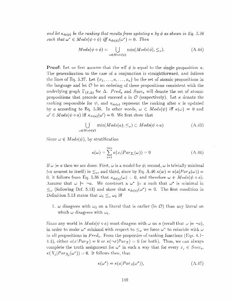
and let K,do(¢>) be the ranking that results from updating K, by c/J as shown in Eq. 5.36 such thatw* E Mods(1/;<>c/J) iffK,do(¢>)(w*) = 0. Then

Mods ( 1/J <> cP) = u min( Mods( cP), s;w ). (A.44) wEMods('if;)

Proof: Let us first assume that the wff cjJ is equal to the single proposition a. The generalization to the case of a conjunction is straightforward, and follows the lines of Eq. 5.37. Let {x1, ... , a, ... , xn} be the set of atomic propositions in the language and let 0 be an ordering of these propositions consistent with the underlying graph r(X,b.) for 6.. Preda and Succa will denote the set of atomic propositions that precede and succeed a in 0 (respectively). Let /'\, denote the ranking responsible for 1/;, and K,do(a) represent the ranking after K, is updated by a according to Eq. 5.36. In other words, w E Mods(1j;) iff K,(w) = 0 and w' E A1ods(1/; <>a) iff K,do(a)(w') = 0. We first show that

u min(Mods(a), s;w) C Mods(1/J <>a) (A.45) wEMods('if;)

Since w E JM ods( 1/J), by stratification

't=n

K,(w) = ~K,(xi!Parx;(w)) = 0 (A.46) i=l

If w I= a then we are done: First, w is a model for c/J; second, w is trivially minimal (or nearest to itself) in s:;w, and third, since by Eq. A.46 K,(w) = K,(a!Pm·A(w)) =

0, it follows from Eq. 5.36 that K,do(a)(w) = 0, and therefore wE Afod.s(l/J <>a). Assume that w I= •a. We construct a w* a such that w* is minima.l in s;w (following Def. 5.13) and show that K,do(a)(w*) = 0. The first condition in Definition 5.13 states that w1 s;w w2 iff

1. w disagrees with w2 on a literal that is earlier (in 0) than any literal on which w disagrees with w1 .

Since any world in Mods ( 1/J <>a) must disagree with w on a (recall that w I= •a), in order to make w* minimal with respect to s;w we force w* to coincide with w in all propositions in Preda. From the properties of ranking functions (Eqs. 4.1-4.:1), either K,(x!Parx) = 0 or K,(•x!Parx) = 0 (or both). Thus, we can always complete the truth assignment for w* in such a way that for every .Tj E Sacca, K,(Xj1Parx

1(w*)) = 0. It follows then, that

(A.47)

140

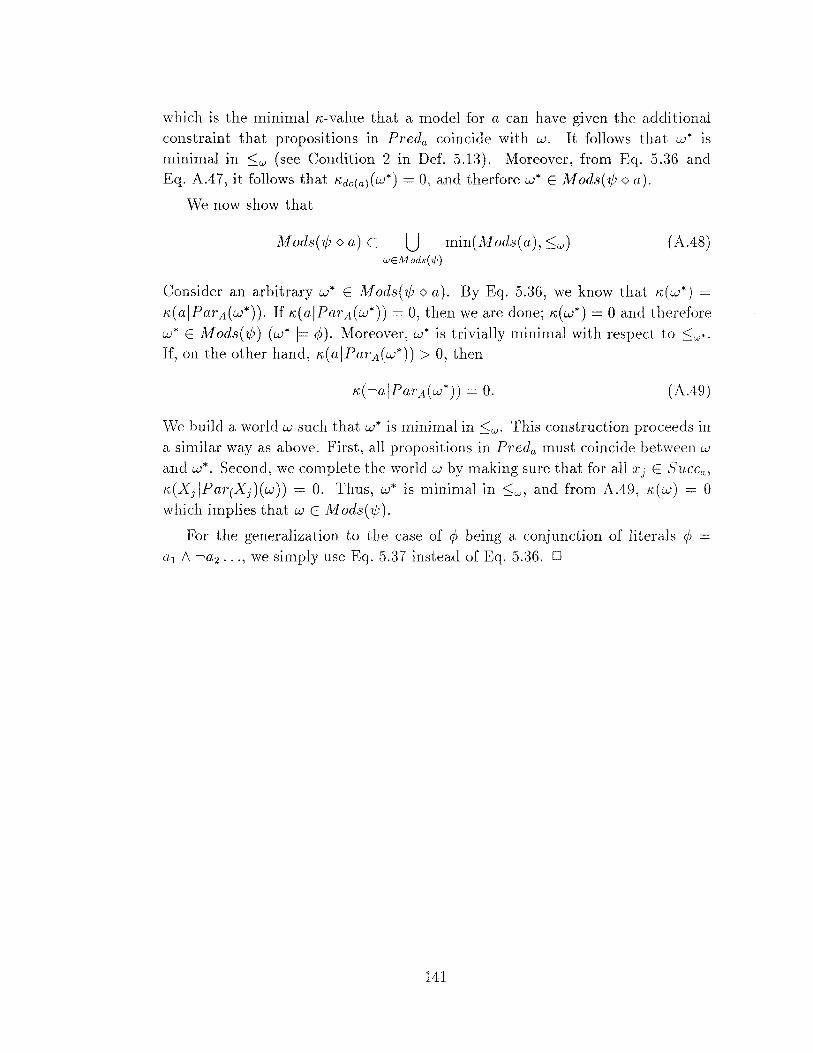
which is the minimal ~>:-value that a model for a can have given the additional constraint that propositions in Preda coincide with w. It follows that w* is minimal in :::;w (see Condition 2 in Def. 5.13). Moreover, from Eq. 5.36 and Eq. A.47, it follows that Kdo(a)(w*) = 0, and therfore w* E _Mods('¢ 0 a).

We now show that

Mods ( '¢ <> a) C u min(Mods(a), :s;w) (A.48) wEMods(,P)

Consider an arbitrary w* E Mods('¢ 0 a). By Eq. 5.36, we know that ~>:(w*) =

~>:(aiParA(w*)). If ~>:(aiParA(w*)) = 0, then we are clone; ~>:(w*) = 0 and therefore w* E Mods('¢) (w* f= c/J). Moreover, w* is trivially minimal with respect to :::;w*· If, on the other hand, ~>:(aiParA(w*)) > 0, then

(A.49)

We build a world w such that w* is minimal in :::;w. This construction proceeds in a similar way as above. First, all propositions in Preda must coincide between w and w*. Second, we complete the world w by making sure that for all Xj E SZLcca, ~>:(XjiPar(Xj)(w)) = 0. Thus, w* is minimal in :::;w, and from A.49, ~>:(w) = 0 which implies that wE Mods('¢).

For the generalization to the case of cjJ being a conjunction of literals cjJ =

a1 1\ -.a2 •• . , we simply use Eq. 5.37 instead of Eq. 5.36. D

141

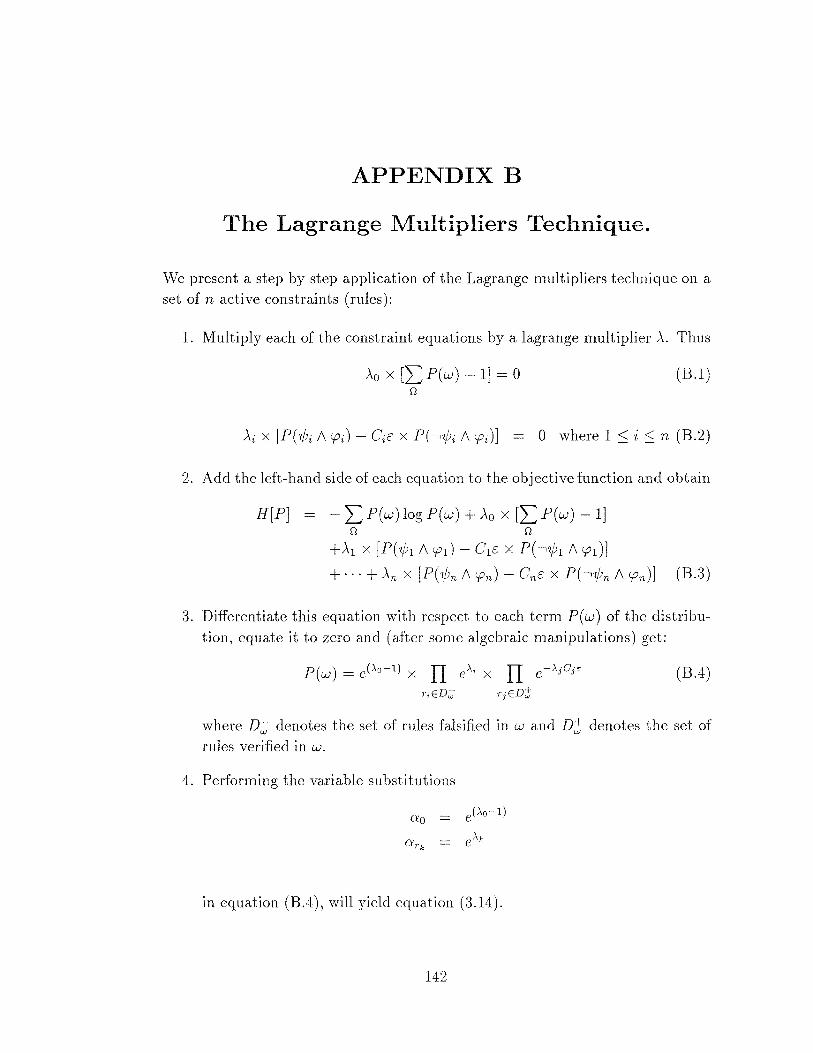
APPENDIX B

The Lagrange Multipliers Technique.

We present a step by step application of the Lagrange multipliers technique on a set of n active constraints (rules):

1. Multiply each of the constraint equations by a lagrange multiplier A. Thus

Ao x [l:::P(w) 1] = 0 (13.1) 0

2. Add the left-hand side of each equation to the objective function and obtain

H[P] = - l:P(w)logP(w) + Ao x [LP(w) -1] 0 0

+A1 x [P( ~1 A so1) - C1c: x P( '~1 A sod]

+···+An x [P( ~n 1\ SOn) Cnc: x P( '~n 1\ SOn)] (B.3)

3. Differentiate this equation with respect to each term P( w) of the distribu­tion, equate it to zero and (after some algebraic manipulations) get:

P(w) = e(>-o-1) X IT e"'i X IT e->-jCje: (B.4) TiED;;; TjED;!;

where D::; denotes the set of rules falsified in w and D;;; denotes the set of rules verified in w.

L1. Performing the variable substitutions

in equation (B.4), will yield equation (3.14).

142

REFERENCES

[1] E. W. Adams. Probability and the logic of conditionals. In J. Hintikka and P. Suppes, editors, Aspects of Inductive Logic. North Holland, Amsterdam, 1966.

[2) E. W. Adams. The Logic of Conditionals. D.Reidel, Dordrecht, Nether­lands, 1975.

[3] C. Alchourr6n, P. Gardenfors, and D. Makinson. On the logic of theory change: Partial meet contraction and revision functions. Journal of Sym­

bolic Logic, 50:510-530, 1985.

[4] A. Anderson and N. Belnap. Entailment: The Logic of Relevance and

Necessity (Vol. 1). Princeton University Press, Princeton N.J., 197.5.

[5] M. Aoki. Introduction to Optimization Techniques. The McMillan Com­pany, New York, 1971. Chapter 5.

[6] F. Bacchus. Representing and Reasoning with Probabilistic Knowledge, A Logical Approach to Probabilities. The MIT Press, Cambridge., 1991.

[7] F. Bacchus, A. Grove, J. Halpern, and D. Koller. Statistical foundations of default reasoning indiference and irrelevance. In Proceedings of the

Fou1·th International Workshop on Nonmonotonic Reasoning, pages 1-12, Vermont, 1992.

[8] A. B. Baker. Nomonotonic reasoning in the framework of situation calculus. Artificial Intelligence, 49:5-23, 1991.

[9] R. Ben-Eliyahu. NP-complete problems in optimal horn clauses satisfiabil­ity. Technical Report R-158, Cognitive systems lab, UCLA, 1990.

[10] R. Ben-Eliyahu and R. Dechter. Propositional semantics for default logic. In Proceedings of the Fourth International Workshop on Nonmonotonic

Reasoning, pages 13-27, Vermont, 1992.

[11] R. Ben-Eliyahu and R. Dechter. Propositional semantics for disjunctive logic programs. In Proceedings of the 1992 Joint International Conference

and Symposium on Logic Programming (in press), Washington, D.C., 1992.

[12] M. Born. Natural Philosophy of Cause and Chance. Clarendon Press, Oxford, 1949.

143

[13] C. Boutilier. Default priorities as epistemic entrenchment. Technical report krr-tr-91-2, University of Toronto, 1991.

[14] C. Boutilier. Conditional logics for default reasoning and belief revision. Ph.D. dissertation, University of Toronto, 1992. Also Technical Report 91-1, Department of Computer Science, University of British Columbia.

[15] C. Boutilier. What is a default priority? In Proceedings of the Canadian

Conference on Artificial Intelligence, pages 140-147, Vancounver, 1992.

[16] G. Brewka. Preferred subtheories: An extended logical framework for de­fault reasoning. In Proceedings of the International Joint Conference in

Artificial Intelligence (IJCAI-89 ), Detroit, 1989.

[17) G. Brewka. Cumulative default logic: In defense of nonmonotonic inference rules. Art~ficial Intelligence, 50:183-205, 1991.

[18) P. Cheeseman. A method of computing generalized bayesian probability values for expert systems. In Proceedings of the International Joint Con­

ference on AI (IJCAI-83), pages 198-202, Karlsruhe, W. Germany, 1983.

[19] M. Dalal. Investigations into a theory of knowledge base revision: Prelimi­nary report. In Pmceedings of the Seventh National Conference on Artificial Intelligence, pages 4 75-4 79, 1988.

[20] R. Dechter and J. Pearl. Network-based heuristics for constraint satisfac­tion problems. Artificial Intelligence, 34:1-38, 1987.

[21] R. Dechter and J. Pearl. Directed constraint networks: A relational frame­work for causal modeling. In Proceedings of the International Joint Con­

ference in Artificial Intelligence (IJCAI-91), pages 1164-1170, Australia, 1991.

[22] A. del Val and Y. Shoham. Deriving properties of belief update from the­ories of acion. In Proceedings of American Association for A1'tijicial Intel­

ligence Conference, pages 584-589, San Jose, California, 1992.

[23] J. P. Delgrande. An approach to default reasoning based on a first-order conditional logic: Revised report. Artificial Intelligence, 36:63-90, 1988.

[24] J.P. Delgrande and W. K. Jackson. Default logic revisited. In Pmceedings

of Principles of Knowledge Representation and Reasoning, pages 118--127, Cambridge, MA, 1991.

144

[25] W. Dowling and J. Gallier. Linear-time algorithms for testing the satis­fiability of propositional Horn formulae. Journal of Logic Programming,

3:267-284, 1984.

[26] J. Doyle. Rationality and its roles in reasoning. In Proceedings of the

American Association for Artificial Intelligence Conference, pages 1093-1100, Boston, 1990.

[27] J. Doyle. Rational belief revision (preliminary report). In Proceedings

of Principles of Knowledge Representation and Reasoning, pages 163-174, Cambridge, MA, 1991.

[28] D. Dubois and H. Prade. Possibility Theory: An Approach to Computerized

Processing of Uncertainty. Plenum Press, New York, 1988.

[29] D. W. Etherington. Formalizing nonmonotonic reasoning systems. A1·tifi­

cial Intelligence, 31:41-85, 1987.

[30] D. W. Etherington and R. Reiter. On inheritance hierarchies with excep­tions. In Proceedings of American Association for Artificial Intelligence

Confe1'ence, pages 104-108, Washington D.C., 1983.

[31] R. Fagin, J. D. Ullman, and M. Vardi. On the semantics of updates in databases. In Proceedings of the 2nd ACM SIGACT-SIGJ\!IOD-SIGART

Symposium on Principles of Database Systems, pages 352-365, 1983.

[32] D. Gabbay. Theoretical foundations for nonmonotonic reasoning in expert systems. In K. R. Apt, editor, Logic and Models of Concurrent Systems.

Springer-Verlag, Berlin, 1985.

[33] P. Giirdenfors. Knowledge in Flux: Modeling the Dynamics of Epistemic

States. MIT Press, Cambridge, 1988.

[34] P. Giirdenfors. Nonmonotonic inferences based on expectations: A prelim­inary report. In Principles of Knowledge Representation and Reasoning:

Proceedings of the Second International Conference, pages 585-590, Boston, 1991.

[35] H. A. Geffner. On the logic of defaults. In Proceedings of AAAI-88, pages 449-454, St. Paul, Minnesota, 1988.

[:36] H. A. Geffner. Default Reasoning: Causal and Conditional Theories. MIT Press, Cambridge, MA, 1992.

145

[37] H. A. Geffner and J. Pearl. A framework for reasoning with defaults. In H. Kyburg, R. Loui, and G. Carlson, editors, Knowledge Representation

and Defeasible Reasoning, pages 245-265. Kluwer Academic Publishers, London, 1990.

[38] H. A. Geffner and J. Pearl. Conditional entailment: Bridging two ap­proaches to default reasoning. Artificial Intelligence, 53:209-244, 1992.

[39] D. Geiger, A. Paz, and J. Pearl. Learning simple causal structures. Journal

of Intelligent Systems, 50:510-530, 1990.

[40] M. Gelfond. On stratified autoepistemic theories. In Proceedings of AAAI-

87, pages 207-211, Seattle, Washington, 1987.

[41] M. Gelfond. Autoepistemic logic and formalization of commonsense rea­soning (preliminary report). In M. Reifrank et. al., editor, Proceedings

of the Second International Workshop on Nonmonotonic Reasoning, pages 177-186, Berlin, Germany, 1989. Springer Lectures in Computer Science.

[42] M. Gelfond and V. Lifschitz. The stable model semantics for logic program­ming. In Proceedings of the Fifth International Conference and Symposium

on Logic Programming, pages 1070-1080, Cambridge, MA, 1988.

[43] M. Gelfond, H. Przymusinska, V. Lifschitz, and M. Truszczynski. Disjunc­tive defaults. In KR-91: Proceedings of the 2nd international conference

on principles of knowledge representation and reasoning, pages 230-237, Cambridge,MA, 1991.

[44] M. Ginsberg. Counterfactuals. Artificial Intelligence, 30:35-79, 1986.

[45] M. Ginsberg. Readings in Nonmonotonic Reasoning. Morgan Kaufmann, San Mateo, CA, 1987.

[46] M. Ginsberg. Multivalued logics: A uniform approach to artificial intelli­gence. Computational Intelligence, 4:265-316, 1988.

[47] M. Goldszmidt, P. Morris, and J. Pearl. A maximum entropy approach to nonmonotonic reasoning. In Proceedings of American Association for Arti­

ficial Intelligence Conference, pages 646-652, Boston, MA, 1990. Extended version to appear in IEEE Transactions on Pattern Analysis and Machine

Intelligence, 1992.

146

[48) M. Goldszmidt and J. Pearl. On the relation between rational closure and system Z. In Third Intemational Workshop on Nonmonotonic Reasoning,

pages 130-140, South Lake Tahoe, 1990.

[49) M. Goldszmidt and J. Pearl. On the consistency of defeasible databases. Artificial Intelligence, 52:121-149, 1991.

[50] M. Goldszmidt and J. Pearl. System z+: A formalism for reasoning with variable strength defaults. In Pmceedings of American Association for Ar­

tificial Intelligence Conference, pages 399-404, Anaheim, CA, 1991.

[51) M. Goldszmidt and J. Pearl. Extending system-Z with negated defaults. Technical Report TR-184, University of California Los Angeles, Cognitive Systems Lab., Los Angeles, 1992.

[52) M. Goldszmidt and J. Pearl. Rank-based systems: A simple approach to belief revision, belief update, and reasoning about evidence and actions. In Principles of Knowledge Representation and Reasoning: Pmceedings of the

Third Intemational Conference (in press), Boston, 1992.

[.53) M. Goldszmidt and J. Pearl. Reasoning with qualitative probabilities can be tractable. In Pmceedings of the gth Conference on Uncertainty in AI,

pages 112-120, Stanford, 1992.

[.54) M. Goldszmidt and J. Pearl. Stratified rankings for causal relations. In Proceedings of the Fourth International Workshop on Nonmonotonic Rea­

soning, pages 99-110, Vermont, 1992.

[5.5] G. Gottlob. Complexity results for nonmonotonic logics. In Proceedings

of the Fourth Intemational Workshop on Nonmonotonic Reasoning, pages 111-125, Vermont, 1992.

[.56] G. Grahne, A. Mendelzon, and R. Reiter. On the semantics of belief revision systems. In Proceedings of the Fourth Conference of Theoretical Aspects of Reasoning About Knowledge, pages 132-142, Moterrey, CA, 1992.

[57) S. Hanks and D. McDermott. Non-monotonic logics and temporal projec­tion. Artificial Intelligence, 33:379-412, 1987.

[58) J. F. Harty and R. H. ThmTlason. Mixing strict and defeasible inheritance. In Pmceedings of AAAI-88, pages 427-432, St. Paul, Minnesota, 1988.

[59] E. Horvitz, J. Breese, and M. Henrion. Decision theory in expert systems and AI. Intemational Journal of Approximate Reasoning, 2:247-302, 1988.

147

[60] D. Hunter. Causality and maximum entropy updating. International lmtr­nal of Approximate Reasoning, 3:87-114, 1989.

[61] D. Hunter. Parallel belief revision. In Shachter, Levitt, Kanal, and Lem­mer, editors, Uncertainty in Artificial Intelligence (Vol. 4}, pages 241-252. North-Holland, Amsterdam, 1990.

[62] D. Hunter. Graphoids and natural conditional functions. International Journal of Approximate Reasoning, 5:489-504, 1991.

[63] E. Jaynes. Where do we stand on maximum entropy? In R. Levine and M. Tribus, editors, The Maximum Entropy Formalism. MIT Press, Cam­bridge, 1979.

[64] R. Jeffrey. The Logic of Decision. University of Chicago Press, Chicago, IL, 1983.

[65] H. Katsuno and A. Mendelzon. On the difference between updating a knowledge base and revising it. In Principles of Knowledge Representation and Reasoning: Proceedings of the Second International Conference, pages 387-394, Boston, 1991.

[66] H. Kautz and B. Selman. Hard problems for simple default logics. Artificial

Intelligence, 49:243-279, 1991.

[67] K. Konolige. On the relation between default logic and autoepistemic logic. A rtzficial Intelligence, 3.5:343-382, 1988.

[68] K. Konolige. Abduction versus closure in causal theories. Artificial Intel­

ligence, .53:255-272, 1992. (Research Note).

[69] S. Kraus, D. Lehmann, and M. Magidor. Nonmonotonic reasoning, pref­erential models and cumulative logics. A1'tificial Intelligence, 44:167-207, 1990.

[70] T. Krishnaprasad, M. Kiefer, and D. Warren. On the circumscriptive se­mantics of inheritance networks. In Z. Ras and L.Saitta, editors, Method­

ologies for Intelligent Systems 4. North Holland, New York, NY, 1989.

[71] S. Lauritzen and D. Spiegelhalter. Local computations with probabilities on graphical structures and their applications to expert systems. Royal

Statistical Society, 50:1.54-227, 1988.

148

[72] D. Lehmann. What does a conditional knowledge base entail? In Pro­

ceedings of Principles of Knowledge Representation and Reasoning, pages 212-222, Toronto, 1989.

[73] D. Lehmann and M. Magidor. Preferential logics: The predicate calculus case. In Proceedings of Theoretical Aspects of Reasoning about Knowledge,

pages 57-72. Morgan Kaufmann, San Mateo, CA, 1990.

[74] D. Lehmann and M. Magidor. What does a conditional knowledge base entail? Artificial Intelligence, 55:1-60, 1992.

[75] H. J. Levesque. All I know: A study in autoepistemic logic. Artificial

Intelligence, 42:263-309, 1990.

[76] D. Lewis. Causation. The Journal of Philosophy, 70:556-567, 1973.

[77] D. Lewis. Probabilities of conditionals and conditional probabilities. Philo­

sophical Review, 85:297-315, 1976.

[78] V. Lifschitz. Computing circumscription. In Proceedings of the InteTna­

tional Joint Conference on AI (IJCAI-85), pages 121-127, Los Angeles, CA, 1985.

[79] V. Lifschitz. Formal theories of action. In M. Ginsberg, editor, Readings in

Nonmonotonic Reasoning, pages 410-432. Morgan Kaufmann, San Mateo, 1987.

[80) V. Lifschitz. Pointwise circumscription. In M. Ginsberg, editor, Readings in

Nonmonotonic Reasoning, pages 410-432. Morgan Kaufmann, San Mateo, 1987.

[81] V. Lifschitz. Circumscriptive theories: a logic-based framework for knowl­edge representation. Journal of Philosophical Logic, 17:391-441, 1988.

[82] V. Lifschitz. On the declarative semantics of logic programs. In Jack Minker, editor, Foundations of Deductive Databases and Logic Programs, pages 89-148. Morgan Kaufmann, 1988.

[83] V. Lifschitz. Open problems on the border of logic and artificial intelligence. Technical report, unpublished manuscript, Department of Computer Sci­ence, Stanford University, 1989.

[84] R. Loui. Defeat among arguments: A system of defeasible inference. In Computational Intelligence, pages 100-106, Canada, 1987.

149

[85] D. Makinson. General theory of cumulative inference. In M.Reinfrank, J. de Kleer, M. Ginsberg, and E. Sandewall, editors, Non-monotonic Rea­

soning. Springer-Verlag, Lecture Notes on Artificial Intelligence 346, Berlin, 1989.

[86] W. Marek. Stable theories in autoepistemic logic. Technical report, Uni­versity of Kentucky, Lexington, KY, 1986.

[87] J. McCarthy. Circumscription a form of non-monotonic reasoning. ATti­

ficial Intelligence, 13:27-39, 1980.

[88] J. McCarthy. Applications of circumscription to formalizing commonsense knowledge. Artificial Intelligence, 28:89-116, 1986.

[89] D. McDermott and J. Doyle. Non-monotonic logic I. Artificial Intelligence,

1:3:41-72, 1980.

[90] R. Moore. Semantical considerations on non-monotonic logic. Artificial

Intelligence, 25:75-94, 1985.

[91] P. Morris. Autoepistemic stable closures and contradiction resolution. In M. Reifrank et. al., editor, Proceedings of the Second International Worlc­

shop on Nonmonotonic Reasoning, pages 60-73, Berlin, Germany, 1989. Springer Lectures in Computer Science.

[92] B. Nebel. Belief revision and default reasoning: Syntax-based approaches. In Proceedings of P7'inciples of Knowledge Representation and Reasoning,

pages 417-428, Cambridge, MA, 1991.

[93] E. Neufeld and D. Poole. Probabilistic semantics and defaults. In Proceed­

ings of the 4th Workshop on Uncertainty in AI, pages 275-281, Mineapolis., 1988.

[94] D. Nute. Conditional logic. In D. Gabbay and F. Guenther, editors, Hand­

book of Philosophical Logic, pages 387-439. D. Reidel, Dordrecht, 1984.

[95] J. Pearl. Deciding consistency in inheritance networks. Technical Report TR-96, University of California Los Angeles, Cognitive Systems Lab., Los Angeles, 1987.

[96] J. Pearl. Embracing causality in formal reasoning. Artificial Intelligence,

35:259-271, 1988.

150

[97] J. Pearl. Probabilistic Reasoning in Intelligent Systems: Networks of Plau­

sible Inference. Morgan Kaufmann, San Mateo, CA, 1988.

[98) J. Pearl. Probabilistic semantics for nonmonotonic reasoning: A survey. In Proceedings of Principles of Knowledge Representation and Reasoning,

pages 505-516, Toronto, 1989.

[99] J. PearL Jeffrey's rule, passage of experience and neo-Bayesianism. In R. Parikh, editor, Defeasible Reasoning and Knowledge Representation,

pages 121-135. Kluwer Publishers, San Mateo, 1990.

[100] J. Pearl. System Z: A natural ordering of defaults with tractable applica­tions to default reasoning. In Proceedings of Theoretical Aspects of Reason­

ing about Know ledge, pages 121-135. Morgan Kaufmann, San Mateo, CA, 1990.

[101] J. Pearl. Probabilistic semantics for nonmonotonic reasoning: A survey. In Philosophy and AI - Essays at the Interface, pages 157-187. Bradford Books/MIT Press, Cambridge, MA, 1991.

[102] .J. Pearl. Epsilon-semantics. In Encyclopedia of Artificial Intelligence, pages 468-475. Wiley Interscience, New York, 1992. Second Edition.

[103] .J. Pearl and T. Verma. A theory fo inferred causation. In Proceedings

of Principles of I< now ledge Representation and Reasoning, pages 441-452, Cambridge, MA, 1991.

[104] D. Poole. On the comparison of theories: Preferring the most specific expla­nation. In Proceedings of Intcr·national Confe?'ence on Artificial Intelligence

(IJCAI-85), pages 144-147, Los Angeles, California, 1985.

[105] D. Poole. A logical framework for default reasoning. Artificial Intelligence,

36:27-4 7, 1988.

[106] D. Poole. Decision-theoretic defaults. In Proceedings of the Canadian Con­

ference on Artificial Intelligence, pages 190-197, Vancounver, 1992.

[107] M. Reifrank, 0. Dressler, and G. Brewka. On the relation between truth maintenance and autoepistemic logic. In Proceedings of the International

Joint Conference in Artificial Intelligence (IJCAI-89), pages 1206-1212, Detroit, 1989.

[108] R. Reiter. A logic for default reasoning. Artificial Intelligence, 13:81-132, 1980.

151

[109] R. Reiter. Nonmonotonic reasoning. Annual Reviews of Computer Science, 2:147-186, 1987.

[110] R. Reiter. A theory of diagnosis from first principles. Artificial Intelligence,

32:97-130, 1987.

[111] R. Reiter. On integrity constraints. In Proceedings of Theoretical Aspects of Reasoni·ng about Knowledge, pages 97-111. Morgan Kaufmann, Pacific Grove, CA, 1988.

[112] R. Reiter and G. Criscuolo. Some representational issues in default reason­ing. International Journal of Computers and Mathematics, 9:1-13, 1983.

[113] K. Satoh. A probabilistic interpretation for lazy nonmonotonic reasoning. In Proceedings of American Association for Artificial Intelligence Confer­

ence, pages 659-664, Boston, 1990.

[114] P. P. Shenoy. On Spohn's rule for revision of beliefs. International Journal

of App·roximate Reasoning, 5(2):149-181, 1991.

[115] P. P. Shenoy and G. Shafer. Axioms for probability and belief-function propagation. In G. Shafer and J. Pearl, editors, Readings in Uncertain

Reasoning, pages 575-610. Morgan Kaufmann, San Mateo, 1990.

[116] Y. Shoham. Chronological ignorance: Time, necessity, and causal theories. In Proceedings of American Association for Artificial Intelligence Confer­

ence, pages 389-393, Philadelphia, 1986.

[117] Y. Shoham. Nonmonotonic logics: Meaning and utility. In Proceedings of

International Conference on AI (IJCAL87), pages 388-393, Milan, Italy, 1987.

[118] Y. Shoham. Reasoning About Change: Time and Causation from the Stand­point of Artificial Intelligence. MIT Press, Cambridge, Mass., 1988.

[119] D. Spiegelhalter and S. Lauritzen. Sequential updating of conditional prob­abilities on directed graphical structures. Networks, 20:579-605, 1989.

[120] W. Spohn. Ordinal conditional functions: A dynamic theory of epistemic states. In W. L. Harper and B. Skyrms, editors, Causation in Decision, Be­

lief Change) and Statistics, pages 105-134. Reidel, Dordrecht, Netherlands,

1988.

152

[121] L. Stein and L. Morgenstern. Motivated action theory: A formal theory of causal reasoning. Technical report cs-89-12, Department of Computer Science, Brown University, 1989. A shorter version in Proceedings AAAI-88, pages 518-523.

[122] D. Touretzky. The Mathematics of Inheritance Systems. Morgan Kauf­mann, San Mateo, 1986.

[123] M. Tribus. Rational Descriptions) Decisions and Designs. Pergamon, Elmsford, NY, 1969.

[124] J. von Neumann and 0. Morgenstern. Theory of Games and Economic

Behavior. Princeton University Press, Princeton, NJ, 1947.

[125] M. Wellman. Fm'mulation of Tradeoffs in Planning under Uncertainty.

Pittman, London, 1990.

[126] M. Wellman, J. Breese, and R. Goldman. From knowledge bases to decision models. The Knowledge Engineering Review, 7(1):35-53, 1992.

[127] M. Winslett. Reasoning about action using a possible worlds approach. In Pmceedings of the Seventh American Association fm' Artificial Intelligence

Conference, pages 89-93, 1988.

153