Embed Size (px)
Citation preview

Nonparametric Prior Elicitation with Imprecisely assessed
Probabilities
Alireza Daneshkhah, Jeremy Oakley and Anthony O’Hagan
Department of Probability and Statistics
University of Sheffield, Sheffield, S3 7RH
[email protected], [email protected], [email protected]
February 7, 2006
1 Introduction
A crucial question that might be arisen in the elicitation of the expert’s probability is that is
the expert able to specify the probability with absolute precision? Unfortunately, by reviewing
the statistical and psychological literature, we learned that the most individuals, in particular
the experts, cannot elicit probabilities with absolute precision.
In this report, we present ways to obtain the highest possible level of accuracy in commu-
nication of two individuals while providing these individual preferences.
We acknowledge that we cannot elicit probabilities with absolute precision, and so we
want to investigate what implications this has for our uncertainty about the expert density
function. We would use the non-parametric approach introduced by Oakley and O’Hagan
(2005) to obtain these implications.
There are several factors (see Garthwaite, et al (2005) for details on the cognitive factors)
that caused this issue. One of the most important factor is that it is difficult for any expert
to give precise numerical values for their probabilities, though this is a requirement in most
elicitation schemes.
Consider an example of a political expert stating her probability that candidate A will win
an election. The expert believes that it is ‘very likely’ that a candidate A will win, but ‘not
a certainty’. In providing a probability P (A wins), the expert must now attach a numerical
value to her feeling that the event {A wins} is ‘very likely’. Clearly her stated value will be
subject to rounding error; the expert may only consider the first two decimal places in her
probability for example and will certainly not state P (A wins) = 0.9243461. However, the
1

issue of imprecision goes beyond this. The expert is unlikely to be in the habit of stating
numbers to represent feelings, and may be unsure if their feeling that an event is ‘very likely’
is most appropriately described with a probability of 0.85, 0.9, 0.99 etc. It is reported that
when representing aleatory uncertainty individuals may be content to use precise numerical
methods (i.e. probabilities), but when representing epistemic uncertainty there is then a
preference to use imprecise methods, such as verbal descriptions of uncertainty. So, there are
two sources of uncertainties in the expert’s stated probabilities: 1) the expert only gives a
limited number of probability judgements; 2) we do not believe these judgements are precise.
In the second section of this report, a review of relevant psychological works will be
presented. Section 3 devoted to a review of the Statistical literature related to this issue.
We will develop Oakley and O’Hagan’s idea associated with imprecise probability in Section
4. We apply these results on the data consists of expert’s probabilities derived by a method
called trial roulette throughout of this report.
2 Imprecise Subjective Probabilities: Psychological Perspec-
tive
Olson and Budescu (1997) have empirically reported that most individuals prefer to use pre-
cise numerical estimates to communicate uncertainty about the repeated events with aleatory
uncertainty, but tend to use imprecise methods when communicating the probabilities of
unique events with epistemic uncertainty.
People would gravitate towards more precise modes of communications if they perceive the
available information to be firmer, reliable and valid. This perceived is called strength of the
available information (See Wallsten et al (1993)). They also reported the person’s role in the
communication. They have found that most people prefer to use imprecise terms when they
communicate to others, but prefer others to communicate to them in precise terms, if possible.
Budescu and Karelitz (2003) analysed an asymmetric dyadic communication situation
where one forecaster and one decision maker share a common interest in optimising com-
munication, but they may have different preference for modality of communication proba-
bilistic opinions. They distinguished between three modes of communication: precise (point)
Numerical probability estimates (e.g., 0.60), precise Ranges of numerical values (e.g., (0.55,
0.65)), and Verbal phrases. The three modes can be ranked from the most precise (N) to
the most vague (V).
Our attempt here is to provide a general framework for the translation process and illustrate
the feasibility of the approach introduced by Budescu and Karelitz (2003). They have an-
2

swered to the following question: How to best translate a judgment originally interpreted
in the forecaster’s favorite response mode (N, R, V) to an estimate in the decision maker’s
favorite mode (N, R, V). In this section, we consider only translation from N to N which is
one of the Common modalities discussed by Budescu and Karelitz (2003).
The criterion of optimality can be considered as the level of similarity1 (or dissimilarity)
between the forecaster’s judgments converted into the decision maker’s favorite mode, and
the decision maker’s natural judgments of the same events in his/her favorite mode.
Dissimilarity between two numbers represented by forecaster and decision maker, nF and
nDM , is defined as the distance between them:
d(nF , nDM ) = |nF − nDM | (1)
It should be pointed out that all the dissimilarity indices are distances.
Translation of the forecaster’s judgment in terms of numbers to the decision maker’s judg-
ment in numbers is the standard case of Bayesian decision analysis. Because numbers are
universal and understandable for everyone, no transformation is then required. As we dis-
cussed in Daneshkhah (2004), most people overestimate low probabilities and underestimate
high probabilities. Thus, we can claim that there exist systematic differences in the degree
to which individuals tend to avoid or favor extreme values.
Budescu and Karelitz (2003) reported that one could quantify this tendency and apply suit-
able stretching (or contacting) transformation. To demonstrate this point, they considered
multiple judges (1, 2, . . . , j, . . . , J) who judge a set of stochastic events (1, 2, . . . , i, . . . , I).
They assumed that:
• All judges have access to the same amount of information, implying that differences in
their judgments are due only to difference in their use of the response scales and random
components.
• All judges naturally distinguish events that are impossible, certain and as likely as not
(probability=0.5).
• Assume an idle judge who is perfectly calibrated and accurate (no random component).
Thus his/her judgments, p1, . . . , pi, match with the events objective probabilities.
1Note that similarity (dissimilarity) is measured in the scale of the target modality, that is, the one that is
favored by the decision maker. So it always relies on commeasurable units or entities.
3

Let denote the assigned probability of judge j to event i by pij . This probability can be
expressed in terms of the objective probability, pi, his/her bias parameter, αj , and the random
component, ǫij which they assume is distributed with µ = 0 and σ > 0. They use the following
model:
Log[pij
(1 − pij)] = αjLog[
pi
(1 − pi)] + ǫij (2)
They assumed that the logit of the judged probabilities is a linear function of the logit of
their objective counterparts.
Individual differences between judges are captured by the parameter αj > 0. They esti-
mated this parameter by using least-square method. They claimed that the model presented
above fits the data well for almost all subjects. For details of this claim and further informa-
tion, see Budescu and Karelitz (2003).
As it is apparent, Psychologists have not provided our needs to specify precise probabil-
ities. In the next section, we first review relevant Statistical papers and we then present a
model to quantify precise probabilities in terms of imprecise (stated) expert’s probabilities.
3 Imprecise Subjective Probabilities: Statistical Perspective
Oakley and O’Hagan (2005) reported a difficulty in the elicitation of expert’s beliefs where
expert is not able to present her2 probability with absolute precision. For example, if the ex-
pert states Pr(θ ∈ A) = 0.6, she might not be able to justify why she stated Pr(θ ∈ A) = 0.6
and not Pr(θ ∈ A) = 0.65 or even Pr(θ ∈ A) = 0.70.
Imprecise probability models are needed in many applications of probabilistic and statis-
tical reasoning. They have been used in the following kinds of problems:
• when there is little information on which to evaluate a probability (see Walley (1991,
1996));
• in robust Bayesian inference, to model uncertainty about a prior distribution (see Berger
(1984), Berger and Berliner (1986), DeRobertis and Hartigan (1981), and Pericchi and
Walley (1991));
2For simplicity, we let the expert be female and the analyst or facilitator be male.
4

• in frequentist studies of robustness, to allow imprecision in a statistical sampling model,
e.g., data from a normal distribution may be contaminated by a few outliers or errors
that come from a completely unknown distribution (see Huber (1981));
• to account for the ways in which people make decisions when they have indeterminate
or ambiguous information (see Einhorn and Hogarth (1985) and Smithson (1989)).
Imprecise probability is used as a generic term to cover all mathematical models which
measure chance or uncertainty without sharp numerical probabilities. It includes both qual-
itative (see Section 2) and imprecise or nonadditive quantitative models. Most probability
judgments in everyday life are qualitative, involving terms like “probably” and “more likely
than”, rather than numerical. There is a large literature on this types of imprecise probability
model.
Our main attempt here to represent the imprecise probability stated by an expert as pre-
cise as possible in numbers. The most relevant work has been reported by Wally (1991) who
considered bounding a Probability P with upper and lower probabilities, P and P respec-
tively. Unfortunately, this still leaves unresolved the issue of how to specify P and P with
absolute precision. Additionally, the expert may also feel that values in the center of the
interval [P , P ] represent their uncertainty more appropriately than values towards the ends
of the interval.
Oakley and O’Hagan (2005) express the reported probability P ∗(θ ∈ A) as the expert’s
true probability plus an additive error which represents the imprecision in the stated proba-
bility as follows,
P ∗(θ ∈ A) = P (θ ∈ A) + ǫ (3)
where ǫ ∼ N(0, τ2) for some appropriate values of τ2.
It should be noticed that normality itself can be considered as a strong assumption, but we
now no longer have absolute lower and upper limits for the true probability P (θ), and it is
also more plausible for the analyst to give greater probability to value P (θ) closer to P ∗(θ).
The variance parameter τ2 now describes the imprecision in the probability assessment, and
may vary for different probability judgments which will be addressed in this report. These
values could be appropriately chosen in consultation with the expert.
In this paper we want to study the following model
p∗i = pi + ǫi, i = 1, . . . , n (4)
5

where p∗i denote imprecise prior probabilities or stated probabilities by an expert, pi denote
p∗i ’s true value (precise probability), and ǫi is considered as a noise which has a distribution
centered around zero and variance that describes the imprecision in the probability assess-
ment.
In this study, we would like to investigate the effect of including the aforementioned noise
in the model described above. We will demonstrate the effect of the noise described above
for an elicitation technique which is originally used in clinical trials by Gore (1987).
Here, we use an elicitation scheme called ‘trial roulette’. This method is very easy to
implement and would allow us to represent the expert’s imprecise probabilities resulting from
rounding. In other words, this approach does not specifically ask for precise probabilities. In
this method, the expert is given a certain number of gaming chips and asked to distribute them
amongst the bins of a histogram. The proportion of chips allocated to a particular bin gives
the expert’s probability of the parameter lying in that bin, though clearly this probability is
then subject to rounding error. We consider the uniform noise for the the mentioned error as
ǫ ∼ U(−a, a), where the length of the interval 2a, denotes the maximum possible error that
would exist in the expert’s stated probabilities.
4 Results
We will present the impact of the imprecise probabilities on the expert’s density for the special
cases when the expert’s true density is either unimodal or skewed distribution. We present
the imprecise probabilities by the trial roulette method throughout this section.
4.1 Bimodal distribution
By the following example, we elicit the expert density function as precise as possible, when
her true density is bimodal.
Example 1 In this example, we assume the expert’s true density is bimodal distribution
(the one that is studied by Oakley and O’Hagan (2005)) and has the following form:
f(θ) = 0.4 × N(−2, 1) + 0.6 × N(1, 2) (5)
where N(µ, σ2) denote the normal distribution with mean, µ, and variance, σ2.
6

Let suppose an expert makes the following statements3 about θ:
Stated Probabilities True Probabilities
p∗1 = Pr(θ ≤ −4) = 0 × 0.05 p1 = Pr(θ ≤ −4) = 0.0092
p∗2 = Pr(−4 ≤ θ ≤ −3) = 1 × 0.05 p2 = Pr(−4 ≤ θ ≤ −3) = 0.0557
p∗3 = Pr(−3 ≤ θ ≤ −2) = 3 × 0.05 p3 = Pr(−3 ≤ θ ≤ −2) = 0.1453
p∗4 = Pr(−2 ≤ θ ≤ −1) = 4 × 0.05 p4 = Pr(−2 ≤ θ ≤ −1) = 0.1735
p∗5 = Pr(−1 ≤ θ ≤ 0) = 3 × 0.05 p5 = Pr(−1 ≤ θ ≤ 0) = 0.1510
p∗6 = Pr(0 ≤ θ ≤ 1) = 3 × 0.05 p6 = Pr(0 ≤ θ ≤ 1) = 0.1648
p∗7 = Pr(1 ≤ θ ≤ 2) = 3.05 p7 = Pr(1 ≤ θ ≤ 2) = 0.1556
p∗8 = Pr(2 ≤ θ ≤ 3) = 2 × 0.05 p8 = Pr(2 ≤ θ ≤ 3) = 0.0967
p∗9 = Pr(3 ≤ θ ≤ 4) = 1 × 0.05 p9 = Pr(3 ≤ θ ≤ 4) = 0.0370
p∗10 = Pr(θ ≥ 4) = 0 × 0.05 p10 = Pr(θ ≥ 4) = 0.0102
where Pr(a ≤ θ ≤ b) = n×0.05 indicates that n chips are allocated to the bin correspond-
ing the interval with endpoints a and b (a < b). It should be noticed that the probability
mentioned above can be defined for any a and b as follows
Pr(a ≤ θ ≤ b) =
∫ b
a
f(θ)dθ
Figure 1 shows the mean and pointwise 95% intervals for the expert density function in
terms of the true probabilities without considering any noise in the data.
We next include noise in the data and study the influence of this noise on the expert
density function.
Now, suppose that the imprecise probabilities (p1, . . . , p10), could be revised by Equation
(4). We consider the following noise that is suggested by Oakley and O’Hagan (2005).
{ǫi}10i=1
iid∼ N(0, [0.1 × (1 − pi)pi]
2) (6)
So probabilities close to 0 or 1 have less absolute imprecision associated with them. The
influence of including this noise in the data is shown in Figure 2.
It should be noticed that we assume weak priors for m and v. The prior distributions for
σ2 and b∗ are given in Equations (8) and (9) (see A.1), respectively. The proposal distribu-
tions we used for the Metropolis-Hastings sampler are:
mt | mt−1 ∼ N(mt−1, 0.01)
3It is assumed that the expert can state Pr(θ < x) for any x.
7

−6 −4 −2 0 2 4 60
0.02
0.04
0.06
0.08
0.1
0.12
0.14
0.16
0.18
Figure 1: The pointwise mean, 2.5th and 97.5th percentiles for the expert density function
(red lines), and the true density function (blue line which is lost between the red lines) when
no noise is considered in data.
−6 −4 −2 0 2 4 60
0.05
0.1
0.15
0.2
0.25
Figure 2: 2.5th, 50th and 97.5th percentiles of f(θ) associated with the revised imprecise
probabilities, pi, where the considered noise has a normal distribution.
8

−6 −4 −2 0 2 4 60
0.05
0.1
0.15
0.2
0.25
Figure 3: 2.5th, 50th and 97.5th percentiles of f(θ) associated with the revised imprecise
probabilities, pi, where a larger noise variance is included.
log(vt) | mt−1, mt, vt−1 ∼ N(log(vt−1), 0.1 × (1 + 5 × |mt − mt−1|))
log(b∗t ) | b∗t−1 ∼ N(log(b∗t−1), 0.01)
log(σ2t ) | σ2
t−1 ∼ N(log(σ2t−1), 0.01)
By comparing Figures 1 and 2 , we can conclude that the inclusion of the noise has sen-
sibly increased posterior uncertainty.
It is apparent that if we use a larger noise variance, e.g., V ar(ǫi) = (0.3 × (1 − p∗i )p∗
i )2, then
expert will be expected to have a smoother, unimodal distribution as shown in Figure 3.
That supports this claim that uncertainty about the expert density will increase as the noise
variance becomes larger.
Gosling (2004) investigated the incorporation of real prior information about b∗ and σ2,
and claimed that it certainly has a strong impact on the results when we reduce the amount
of observations elicited from the expert. Since, we cannot expect to elicit much from the
expert that would be a positive result. He proposed the following prior distributions for b∗
and σ2 inside the boundaries suggested by a figure in his report.
log(b∗) ∼ N(0.47, 0.42)
log(σ2) | b∗ ∼ N(M, S2)
where
M =log(0.31(b∗ − 0.6)2 + 0.11) + log(0.07(b∗ − 0.36)2 + 0.0008)
2,
9

−6 −4 −2 0 2 4 60
0.05
0.1
0.15
0.2
0.25
Figure 4: 2.5th, 50th and 97.5th percentiles of f(θ) with Gosling’s prior distributions for b∗
and σ2.
S =log(0.07(b∗ − 0.36)2 + 0.0008) − log(0.31(b∗ − 0.6)2 + 0.11)
2Φ−1(0.005).
The pointwise median, 2.5th and 97.5th precentiles of the expert density, by including the
prior distributions described above, is shown in Figure 4.
From what we have demonstrated in the figures above we can conclud that the true den-
sity is not included within the pointwise 95% interval for the expert density function. The
figure below shows that true cumulative distribution function is not either included within
the pointwise 95% interval for the expert distribution function.
It should be noted that according to the nature of the problem (bimodal distribution) the
quality of data derived from the expert is very important. In fact, when the true density is
bimodal, it will be difficult for the method to capture this feature using only imprecise elicited
probabilities, given that the prior expectation is for unimodality. In practice, we would expect
the expert to be able to specify when her distribution is bimodal, and specifically inputting
this information and the location of the modes should improve the fitted distribution.
The similar results will be obtained if we consider the error terms in Equation (4) are uni-
formly distributed (see A.3 for the details associated with this noise), i.e, ǫiiid∼ U(−0.025, 0.025).
The pointwise mean, and 95% intervals of the expert’s density for the aforementioned noise
are shown in Figure 6.
10

−6 −4 −2 0 2 4 60
0.1
0.2
0.3
0.4
0.5
0.6
0.7
0.8
0.9
1
Figure 5: 2.5th, 50th and 97.5th percentiles of F (θ) associated with the revised imprecise
probabilities, pi
−6 −4 −2 0 2 4 60
0.05
0.1
0.15
0.2
0.25
Figure 6: 2.5th, 50th and 97.5th percentiles of f(θ) with Inverted-Gamma prior for σ2 when
ǫiiid∼ U(−0.025, 0.025).
11

0 5 10 15 20 250
0.1
0.2
0.3
0.4
0.5
0.6
0.7truemedianpointwise 99% intervallocationnorthwest
Figure 7: The mean and pointwise 99% intervals for the expert’s density, and the true density
(dotted line) with uniform noise when the imprecise probabilities are rounded to nearest 10%.
4.2 Skewed Distributions
In this section, we assume that the expert’s true density is a unimodal distribution and either
skewed to the right or the left (e.g., Gamma or Beta distribution). Here, we study the influ-
ence of the imprecise probabilities on the expert density. We also only consider the uniform
noise to revise the stated probabilities.
Example 2 (Gamma Distribution) Let assume the expert has the following density
function for θ:
f(θ) = θ exp(−θ)
We also assume that the expert can report P0,1.25, P1.25,2.5, P2.5,3.75, P3.75,5 and P3.75,∞, where
Px,y = P (x ≤ θ ≤ y) =∫ y
xf(θ)dθ. These stated probabilities are usually included the errors.
We will again use MCMC to obtain samples of {m, v, b∗} from their joint posterior distribution
when the inverse gamma distribution is considered as the prior distribution for σ2. The chain
is run for 2000 iterations and the first 1000 runs are discarded to allow for the burn-in period.
Figures 7 and 8 are the plots of the pointwise median, 0.5th and 99.5the percentiles from our
posterior distribution for the density and distribution functions, respectively. Notice that the
expert true density is included in the 99% intervals. In these figures, the stated probabilities
are rounded to nearest 10%.
Our results obtained above are robust with respect to the changes on the hyperparameters
12

0 5 10 15 20 250
0.1
0.2
0.3
0.4
0.5
0.6
0.7
0.8
0.9
1
true CDFpointwise 99% intervallocationnorthwest
Figure 8: The mean and pointwise 99% intervals for the expert’s distribution function, and the
true distribution function (dotted line) with uniform noise when the imprecise probabilities
are rounded to nearest 10%.
of the mentioned prior for σ2 if we do not choose very small values for the hyperparameters.
Figures 9 and 10 are the expert’s density and distribution functions when the prior distribu-
tion on σ2 is, p(σ2) = Ing(0.0002, 0.0001). It can be seen the true density and distribution
functions are not included in the intervals.
Example 3 (Beta Distribution)
One of the most important right-hand tail distribution is Beta distribution. We assume
here that the expert true density is a Beta distribution with the specified hyperparameters de-
temined later. Similar to the example mentioned above, we divide the support of θ in a proper
way into some sub-intervals, and we will again use MCMC to obtain samples of {m, v, b∗} from
their joint posterior distribution when the inverse gamma distribution is considered as the
prior distribution for σ2. Figures 11 and 12 are the plots of the pointwise median, 0.5th and
99.5the percentiles from our posterior distribution for the density and distribution functions,
respectively. In these figures, the stated probabilities are rounded to nearest 10%.
We can conclude the similar results as above that when the hyperparameters of the in-
verse gamma distribution-considered as a prior distribution for σ2- are both very small4, the
4Notice that, when the hyperparameters of the inverse gamma distribution tend to zero, the inverse gamma
distribution tend to the uniform distribution. In fact, in this case, we use a non-informative prior for σ2.
13

0 5 10 15 20 250
0.05
0.1
0.15
0.2
0.25
0.3
0.35
0.4
0.45
0.5truemedianpointwise 99% intervallocationnorthwest
Figure 9: The mean and pointwise 95% intervals for the expert’s density, and the true density
function (dotted line) with uniform noise when p(σ2) = Ing(0.0002, 0.0001).
0 5 10 15 20 250
0.1
0.2
0.3
0.4
0.5
0.6
0.7
0.8
0.9
1true CDFpointwise 99% intervallocationnorthwest
Figure 10: The mean and pointwise 95% intervals for the expert’s distribution, and the true
distribution function (dotted line) with uniform noise when when p(σ2) = Ing(0.0002, 0.0001).
14

0 0.1 0.2 0.3 0.4 0.5 0.6 0.7 0.8 0.9 10
0.2
0.4
0.6
0.8
1
1.2
1.4
1.6
1.8
truemedianpointwise 99% intervallocationnorthwest
Figure 11: The mean and pointwise 99% intervals for the expert’s density, and the true density
(dotted line) with uniform noise when the imprecise probabilities are rounded to nearest 10%.
The prior distribution on σ2 is Ing (2,1).
0 0.1 0.2 0.3 0.4 0.5 0.6 0.7 0.8 0.9 10
0.1
0.2
0.3
0.4
0.5
0.6
0.7
0.8
0.9
1
true CDFpointwise 99% intervallocationnorthwest
Figure 12: The mean and pointwise 99% intervals for the expert’s distribution function, and
the true distribution function (dotted line) with uniform noise when the imprecise probabilities
are rounded to nearest 10%. The prior distribution on σ2 is Ing (2,1).
15
0 0.1 0.2 0.3 0.4 0.5 0.6 0.7 0.8 0.9 10
0.2
0.4
0.6
0.8
1
1.2
1.4
1.6
1.8
truemedianpointwise 99% intervallocationnorthwest
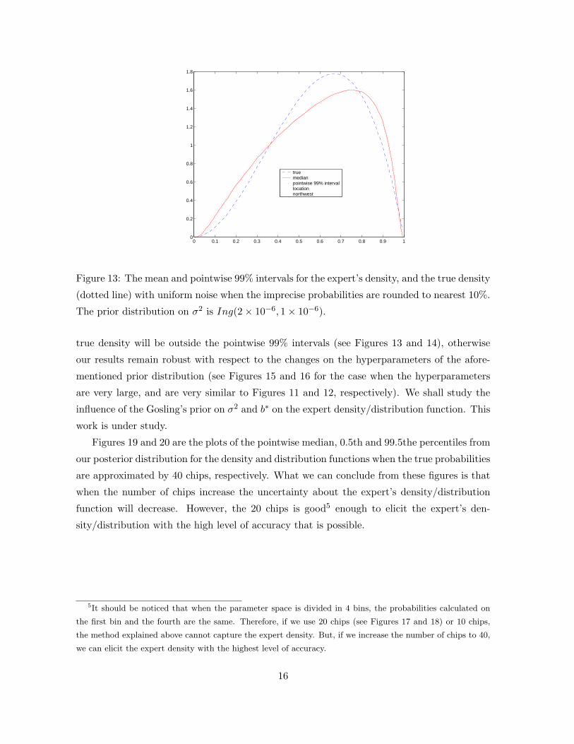
Figure 13: The mean and pointwise 99% intervals for the expert’s density, and the true density
(dotted line) with uniform noise when the imprecise probabilities are rounded to nearest 10%.
The prior distribution on σ2 is Ing(2 × 10⁻⁶, 1 × 10⁻⁶).
true density will be outside the pointwise 99% intervals (see Figures 13 and 14), otherwise
our results remain robust with respect to the changes on the hyperparameters of the afore-
mentioned prior distribution (see Figures 15 and 16 for the case when the hyperparameters
are very large, and are very similar to Figures 11 and 12, respectively). We shall study the
influence of the Gosling’s prior on σ2 and b∗ on the expert density/distribution function. This
work is under study.
Figures 19 and 20 are the plots of the pointwise median, 0.5th and 99.5the percentiles from
our posterior distribution for the density and distribution functions when the true probabilities
are approximated by 40 chips, respectively. What we can conclude from these figures is that
when the number of chips increase the uncertainty about the expert’s density/distribution
function will decrease. However, the 20 chips is good5 enough to elicit the expert’s den-
sity/distribution with the high level of accuracy that is possible.
5It should be noticed that when the parameter space is divided in 4 bins, the probabilities calculated on
the first bin and the fourth are the same. Therefore, if we use 20 chips (see Figures 17 and 18) or 10 chips,
the method explained above cannot capture the expert density. But, if we increase the number of chips to 40,
we can elicit the expert density with the highest level of accuracy.
16

0 0.1 0.2 0.3 0.4 0.5 0.6 0.7 0.8 0.9 10
0.1
0.2
0.3
0.4
0.5
0.6
0.7
0.8
0.9
1
true CDFpointwise 99% intervallocationnorthwest
Figure 14: The mean and pointwise 99% intervals for the expert’s distribution function, and
the true distribution function (dotted line) with uniform noise when the imprecise probabilities
are rounded to nearest 10%. The prior distribution on σ2 is Ing(2 × 10⁻⁶, 1 × 10⁻⁶).
0 0.1 0.2 0.3 0.4 0.5 0.6 0.7 0.8 0.9 10
0.2
0.4
0.6
0.8
1
1.2
1.4
1.6
1.8
2
truemedianpointwise 99% intervallocationnorthwest
Figure 15: The mean and pointwise 99% intervals for the expert’s density, and the true density
(dotted line) with uniform noise when the imprecise probabilities are rounded to nearest 10%.
The prior distribution on σ2 is Ing(2 × 10³, 1 × 10³).
17

0 0.1 0.2 0.3 0.4 0.5 0.6 0.7 0.8 0.9 10
0.1
0.2
0.3
0.4
0.5
0.6
0.7
0.8
0.9
1
true CDFpointwise 99% intervallocationnorthwest
Figure 16: The mean and pointwise 99% intervals for the expert’s distribution function, and
the true distribution function (dotted line) with uniform noise when the imprecise probabilities
are rounded to nearest 10%. The prior distribution on σ2 is Ing(2 × 10³, 1 × 10³).
0 0.1 0.2 0.3 0.4 0.5 0.6 0.7 0.8 0.9 10
0.2
0.4
0.6
0.8
1
1.2
1.4
1.6
1.8
2
Figure 17: The mean and pointwise 99% intervals for the expert’s density, and the true density
(dotted line) with uniform noise when the imprecise probabilities are rounded to nearest 5%.
The prior distribution on σ2 is Ing(2, 1).
18

0 0.1 0.2 0.3 0.4 0.5 0.6 0.7 0.8 0.9 10
0.1
0.2
0.3
0.4
0.5
0.6
0.7
0.8
0.9
1
Figure 18: The mean and pointwise 99% intervals for the expert’s distribution function, and
the true distribution function (dotted line) with uniform noise when the imprecise probabilities
are rounded to nearest 5%. The prior distribution on σ2 is Ing(2, 1).
0 0.1 0.2 0.3 0.4 0.5 0.6 0.7 0.8 0.9 10
0.2
0.4
0.6
0.8
1
1.2
1.4
1.6
1.8
2
truemedianpointwise 99% intervallocationnorthwest
Figure 19: The mean and pointwise 99% intervals for the expert’s density function, and the
true density function (dotted line) with uniform noise when the imprecise probabilities are
rounded to nearest 2.5%. The prior distribution on σ2 is Ing(2, 1).
19

0 0.1 0.2 0.3 0.4 0.5 0.6 0.7 0.8 0.9 10
0.1
0.2
0.3
0.4
0.5
0.6
0.7
0.8
0.9
1
true CDFpointwise 99% intervallocationnorthwest
Figure 20: The mean and pointwise 99% intervals for the expert’s distribution function, and
the true distribution function (dotted line) with uniform noise when the imprecise probabilities
are rounded to nearest 2.5%. The prior distribution on σ2 is Ing(2, 1).
5 Conclusion and Future Works
We have investigated the issue of imprecision in the expert probability assessments. We have
considered the data consists of expert’s summaries obtained by a method called trial roulette.
We have shown that the inclusion of the noise (either normal or uniform) has sensible influ-
ence on the posterior uncertainty and so the expert density. When we add the noise to the
imprecise probabilities (reported by the expert), a smooth and unimodal (especially for the
larger variance noise) distribution for the expert density will be expected.
We have also included Gosling’s prior distributions for σ2 and b∗. However, we were ex-
pected to see different results by the inclusion of his priors, but our data have not supported
his claim and have not shown significant changes for the bimodal distribution. The influence
of this prior for σ2 on the unimoda distributions is under study. Using proper prior for σ2 is
strongly recommended in this study.
Unfortunately, the true density/distribution function is not included within the pointwise
95% interval for the expert density function/distribution function.
Several solutions to explain this issue can be suggested. The first one is about the quality of
data derived from the expert. We believe that if the true density was unimodal, expert would
20

0 10 20 30 40 50 60 70 80 90 100−0.2
0
0.2
0.4
0.6
0.8
1
1.2Autocorrelation in MCMC output
mvb
Figure 21: The autocorrelation in MCMC output associated with {m, v, b∗}.
then provide more accurate information. In fact, when the true density is bimodal, expert
might be unable to specify this point or express right places of two modes. In this situation,
the following question should receive more attention. How should we use trial roulette method
to elicit more reliable information from expert?
The following questions have been addressed in this report, but more works need to be
done here.
• What is an appropriate proper of prior for σ2?
• How sensitive is posterior distribution of f(.) to prior on σ2?
We would also like to make some investigation about the autocorrelation (see Figure 21)
in Markov chain associated with {m, v, b∗}, and find out can this be reduced, especially for
v?
We also like to study the influence of a mixture of normals for the underlying (the analyst)
distribution on the expert density. We expect to see the the true density is included between
the 99% intervals with some degree of uncertainty which seems to be plausible with the noise
considered in the model. This work is under study, and the results would be presented in the
next meetings.
21

A Appendices: Calculation H and A for the model with noise
In this section, we calculate the mean vector and covariance matrix of the Gaussian process
prior for the model represented in Equation (4). We are considering two noises: normal and
uniform.
A.1 Normal Independent Noise
First, we assume the noise terms (given in Equation (4)) are independently distributed as
normal. Now, for the given interval [xi−1, xi], the expert probability is given by
p∗i = Pr(xi−1 ≤ θ ≤ xi) =
∫ xi
xi−1
f(θ)dθ.
This has a normal distribution, with
E(p∗i | u = {m, v, b∗}) = Φ(xi − m
v) − Φ(
xi−1 − m
v)
and
Cov(p∗i , p∗
j | u, σ2) =
| S |1
2 σ2
2πv
∫ xi
xi−1
∫ xj
xj−1
| S |−1
2 exp{−1
2(θ − m, φ − m)S−1(θ − m, φ − m)T }dθdφ
where
S−1 =
(
1+b∗
vb∗− 1
vb∗
− 1vb∗
1+b∗
vb∗
)
Now, if ǫi ∼iid N(0, τ2), then pi has also a normal distribution with
E(pi | u) = E(p∗i | u)
and
Cov(pi, pj | u, σ2) =
{
Cov(p∗i , p∗
j | u, σ2) if i 6= j
V ar(p∗i ) + 1τ2 if i = j
Therefore, the considered noise has influence on the diagonal elements of the covariance ma-
trix.
22

A.2 Normal Dependent Noise
If ǫi’s are dependent on each other as the way we explained above. To determine the distrib-
ution of ǫ | W = 0, we define
M =
(
ǫ
W
)
The variance matrix of M is given by
V ar(M) =
(
D N
NT w
)
where D = V ar(ǫ) = diag(σ21, . . . , σ
2n), NT = Cov(ǫ, W ) = (σ2
1, . . . , σ2n), and w = V ar(W ) =
∑ni=1 σ2
i . Therefore,
{ǫi}ni=1 | (W = 0)
iid∼ N(0, D − N × w−1 × NT ) (7)
A.3 Uniform Noise
But, if we assume that ǫiiid∼ U(−a, a), then computation of H and A would be very difficult
in this case. However, we can compute distribution6 associated with pi’s.
We should consider ǫi as another hyperparameter, and conational on this hyperparameter
the posterior distribution should be revised. Therefore, the hyperparameters are
αn = (m, v, b∗, σ2, ǫ)
where ǫ = {ǫi}ni=1.
Let the data comprise a vector D∗ of elicited summaries such as moments and quantiles
for the original model without considering any noise. In fact, D∗ can be parented as follows
D∗ = {p∗i , i = 1, . . . , n;n∑
i=1
p∗i = 1}
where p∗i =∫ xi
xi−1f(θ)dθ.
The data associated with precise probabilities pi denoted by D and defined as follows
D = {pi = p∗i + ǫi, i = 1, . . . , n;n∑
i=1
pi = 1}.
6It has been proved that the convolution of a Uniform and a Normal distribution results in a quasi-uniform
distribution smeared out as its edge. It might help us to find the distribution of pi, generally, in this situation.
This work is under study.
23

Oakly and O’Hagan (2003) considered the following prior distribution for α = (m, v, σ2, b∗)
p((m, v, σ2, b∗) ∝ v−1σ−2p(b∗)
where p(b∗) will be an informative prior for b∗ expressing the above beliefs.
We consider the following prior distribution on (α, ǫ)
p(m, v, σ2, b∗, ǫ) ∝ v−1p(σ2)p(b∗)p(ǫ)
where p(ǫ) =∏n
i=1(2a)−1I(ǫi)(−a,a), p(σ2) is either informative or uninformative prior distribu-
tions which will be introduced later, and log(p∗) ∼ N(0.65, 0.252).
We also know that D∗ ∼ MV Nn×n(H, σ2A) with the following presentation
p(D∗ | α) ∝ σ−n|A|−1
2 exp{−1
2σ2(D∗ − H)T A−1(D∗ − H)}
It can be easily shown that
p(D | α, ǫ) = p(D∗ + ǫ | α, ǫ)
where
p(D | α, ǫ) ∝ σ−n|A|−1
2 exp{−1
2σ2(D∗ − (H − ǫ))T A−1(D∗ − (H − ǫ))} (8)
The posterior distribution of (α, ǫ) can be easily derived from the multivariate normal likeli-
hood given in Equation (4) for D given (α, ǫ):
p(α, ǫ | D) ∝ v−1σ−n|A|−1
2 exp{−1
2σ2(D∗ − H)T A−1(D∗ − H)} × p(b∗)p(σ2)p(ǫ)
where n denotes the number of elements in D. The posterior marginal distribution of f(θ)
is then the result of integrating its Gaussian process conditional distribution with respect
to this marginal posterior of the hyperparameters. The conditioning on σ2 can be removed
analytically to obtain
p(m, v, b∗, ǫ | D∗) ∝ v−1(σ̂2)−n2 | A |−
1
2 p(ǫ)
We first consider the following distributions as priors for σ2 and b∗, respectively
p(σ2) ∝ (σ2)−(a0+1) exp{−b0
σ2}, (9)
log(b∗) ∼ N(0.65, 0.1252) (10)
The posterior marginal distribution of f(θ) is then the result of integrating its Gaussian
process conditional distribution with respect to this marginal posterior of the hyperparame-
ters.
24

We can then use MCMC to obtain a sample of values of (m, v, b∗, σ2, ǫ) from their joint pos-
terior mentioned above. Finally, given these values, we can sample a density function f(.) at
a finite number of values of θ from the posterior p{f(.) | D, α, ǫ}. Repeating this will give us
a sample of functions from the posterior p{f(.) | D}, and estimates and pointwise bounds for
f(θ) can then be reported.
References
[1] Berger, J. O (1984). The robust Bayesian viewpoint (with discussion). In Robustness of
Bayesian Analysis, J. Kadane (Ed.), North-Holland, Amesterdam.
[2] Berger, J. O., and Berliner. L. M. (1986). Robust Bayes and empirical Bayes analysis
with ǫ-contaminated priors. Ann. Statist., 14,461-486.
[3] Budescu, D. V., Karelitz, T. M. (2003). Inter-personal communication of precise
and imprecise subjective probabilities. The paper is available from WWW URL:
http://www.carleton-scientific.com/isipta/PDF/008.pdf.
[4] Daneshkhah, A. (2004). Psychological Aspects Influencing Elicitation of Subjective Prob-
ability. BEEP’s report.
[5] DeRobertis, L., and Hartigan, J. (1981). Bayesian inference using intervals of measures.
The Annals of Statistics , 9, 235-244. Einhorn,
[6] Einhorn, H. J. and Hogarth, R. M. (1985). Ambiguity and uncertainty in probabilistic
inference. Psychological Review, 92, 433-461.
[7] Gore, S. M. (1987). Biostatistics and the medical Reserach Council. Medical Research
Council News.
[8] Gosling, J. P. (2004). Incorporating prior knowledge into a Gaussian Process Prior. Re-
search Report, Department of Statistics, University of Sheffield.
[9] Huber. P. (1981). Robust Statistics. Wiley, New York.
[10] Oakley, J. and O’Hagan, A. (2005). Uncertainty in prior elicitations: a non-parametric
approach. Research Report No. 521/02 Department of Probability and Statistics, Uni-
versity of Sheffield.
[11] Olson, M. J., and Budescu, D. V. (1997). Patterns of preference for numerical and verbal
probabilities. Journal of Behavioral Decision Making, 10, 117-131.
25

[12] Pericchi, R. L., and Walley, P. (1991). Robust Bayesian credible intervals and prior
ignorance. International Statistical Review, 58, 1-23.
[13] Smithson, M. (1989). Ignorance and Uncertainty: Emerging Paradigms. New York:
Springer-Verlag.
[14] Walley, P. (1991). Statistical Reasoning with Imprecise Probabilities. Chapman and Hall,
London.
[15] Walley, P. (1996). Inferences from multinomial data: learning about a bag of marbels
(with discussion). Journal of the Royal Statistical Society, Series B, 58, 3-57.
[16] Wallsten, T. S., Budescu, D. V., Zwick, R., and Kemp, S. M. (1993). Preferences and
Reasons for Communicating Probabilistic Information in Verbal or Numerical Terms.
Bulletin of the Psychonomic Society, 31:2, 135-138.
26


