Nonparametric ridge estimation

NONPARAMETRIC RIDGE ESTIMATION

By Christopher R. Genovese∗, Marco Perone-Pacifico†,Isabella Verdinelli†, and Larry Wasserman§

Carnegie Mellon University and Sapienza University of Rome

December 20, 2012

We study the problem of estimating the ridges of a density function. Ridgeestimation is an extension of mode finding and is useful for understanding thestructure of a density. It can also be used to find hidden structure in point clouddata. We show that, under mild regularity conditions, the ridges of the kerneldensity estimator consistently estimate the ridges of the true density. Whenthe data are noisy measurements of a manifold, we show that the ridges areclose and topologically similar to the hidden manifold. To find the estimatedridges in practice, we adapt the modified mean-shift algorithm proposed byOzertem and Erdogmus (2011). Some numerical experiments verify that thealgorithm is fast and accurate.

∗Research supported by NSF Grant DMS-0806009.†Research supported by Italian National Research Grant PRIN 2008.‡Research supported by Italian National Research Grant PRIN 2008.§Research supported by NSF Grant DMS-0806009, Air Force Grant FA95500910373.AMS 2000 subject classifications: Primary 62G05, 62G20; secondary 62H12Keywords and phrases: ridges, density estimation, manifold learning

1

arX

iv:1

212.

5156

v1 [

mat

h.ST

] 2

0 D

ec 2

012

http://www.imstat.org/aos/

2 GENOVESE, PERONE-PACIFICO, VERDINELLI, WASSERMAN

CONTENTS

1 Introduction . . . . . . . . . . . . . . . . . . . . . . . . . . . . . . . 4

2 Model . . . . . . . . . . . . . . . . . . . . . . . . . . . . . . . . . . 8

3 Technical Background . . . . . . . . . . . . . . . . . . . . . . . . . 9

3.1 Distance Function and Hausdorff Distance . . . . . . . . . . . 9

3.2 Topological Concepts . . . . . . . . . . . . . . . . . . . . . . . 10

3.3 Matrix Theory . . . . . . . . . . . . . . . . . . . . . . . . . . 11

4 Ridges . . . . . . . . . . . . . . . . . . . . . . . . . . . . . . . . . . 14

4.1 Definitions . . . . . . . . . . . . . . . . . . . . . . . . . . . . . 14

4.2 Differentials . . . . . . . . . . . . . . . . . . . . . . . . . . . . 16

4.3 Assumptions . . . . . . . . . . . . . . . . . . . . . . . . . . . 18

4.4 Quadratic Behavior . . . . . . . . . . . . . . . . . . . . . . . . 19

4.5 Stability of Ridges . . . . . . . . . . . . . . . . . . . . . . . . 21

5 Ridges of Density Estimators . . . . . . . . . . . . . . . . . . . . . 23

6 Ridges as Surrogates for Hidden Manifolds . . . . . . . . . . . . . . 25

7 Subspace Constrained Mean Shift . . . . . . . . . . . . . . . . . . . 29

8 Implementation and Examples . . . . . . . . . . . . . . . . . . . . 30

9 Conclusion . . . . . . . . . . . . . . . . . . . . . . . . . . . . . . . 31

Appendix: Proof of Lemma 10 . . . . . . . . . . . . . . . . . . . . . . 36

References . . . . . . . . . . . . . . . . . . . . . . . . . . . . . . . . . . 43

Author’s addresses . . . . . . . . . . . . . . . . . . . . . . . . . . . . . 44

RIDGE ESTIMATION 3

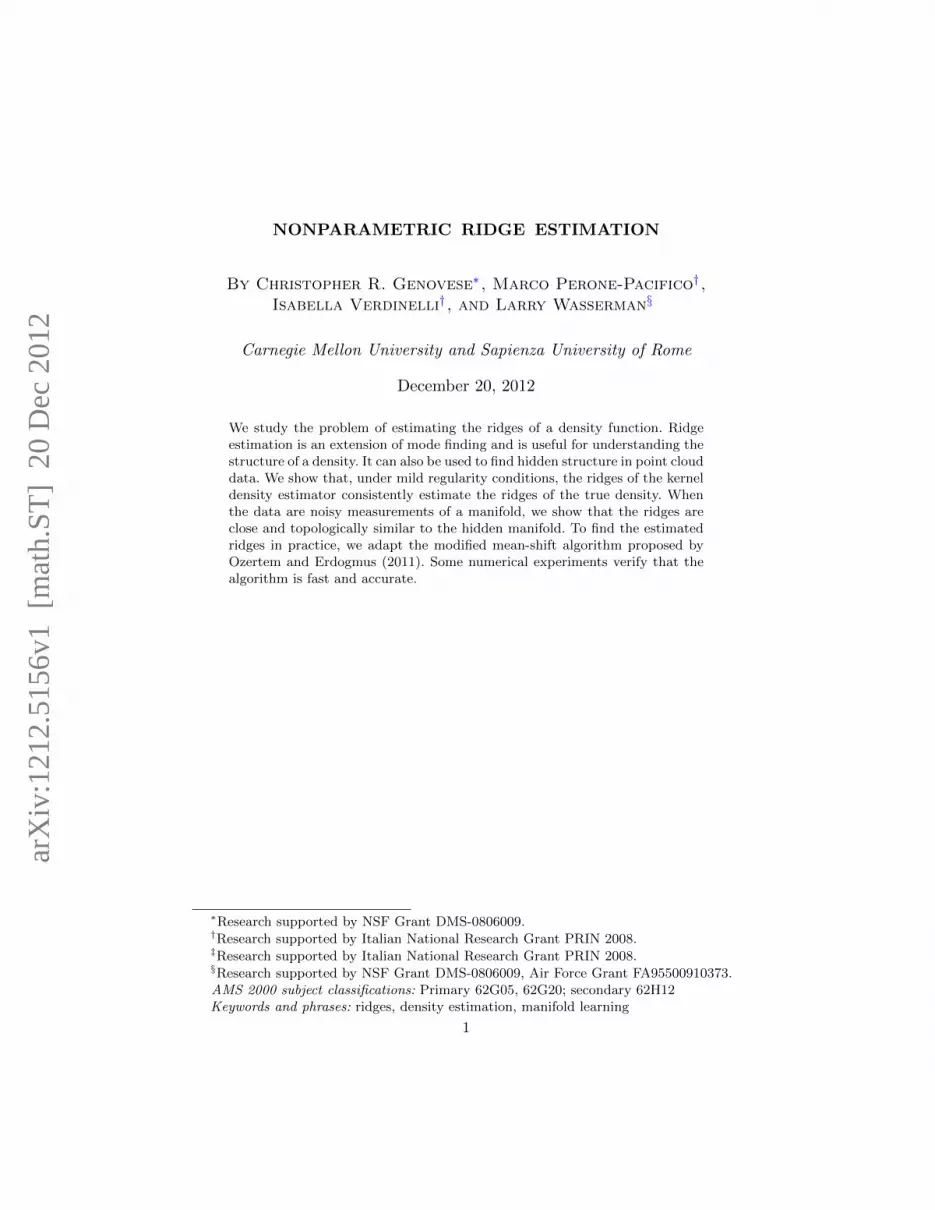
Notation

P distribution of X ∈ RDp(x) density of P ; x ∈ RD

g(x) gradient of p

H(x) = U(x)Λ(x)U(x)T Hessian of p and its spectral decomposition

U(x) = [V�(x) : V (x)] eigenvectors of H

L(x) = V (x)V (x)T projector onto the local normal space

G(x) = L(x)g(x) projected gradient

R d-dimensional ridge of p where 0 ≤ d < D

π(t) integral curve (path to ridge)

γ(s) integral curve parameterized by arclength s.L,

.g derivative along the curve γ(s)

S the set of all symmetric D ×D matrices

L† Frechet derivative of L : S → Sφσ(x) Gaussian density, mean 0 covariance σ2I

pσ(x) =∫M φσ(x− z)dW (z) density of X when there is a hidden manifold M


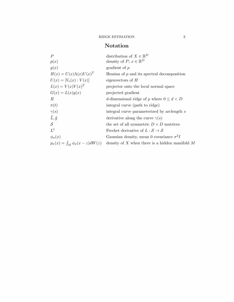
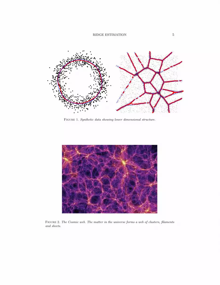
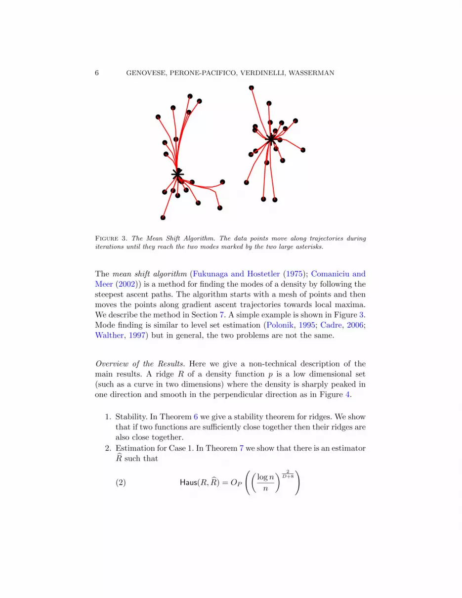
1. Introduction. In many problems, multivariate data have some in-trinsic low dimensional structure. Examples are clusters, manifolds, inter-secting manifolds et cetera. See Figures 1 and 2. These features may showup in the density as modes, ridges and hyper-ridges. In this paper we studya method for finding these features. We consider two cases:

Case 1: (The Unstructured Case): We observe a sample X1, . . . , Xn froma density p. The goal is to find the ridges (and hyper-ridges) of p.

Case 2: (The Hidden Manifold Case): We observe a sample X1, . . . , Xnfrom a density p. There is an underlying hidden manifold M and there is amodel relating the manifold to the ridges of the density. The goal is to estimatethe ridges and relate the ridges to M . We show that the ridge R is a surrogatefor M , meaning that, under appropriate conditions, R is close to M and has asimilar topology as M . The manifold can only be estimated at a logarithmicrate (Genovese et al., 2012b) but the ridge can be estimated at a polynomialrate.

Our goal is to provide a theoretical framework for estimating ridges. In par-ticular we show that the ridges of a kernel density estimator consistentlyestimate the ridges of the density and we find the rate of convergence. Thisleaves open the question of how to locate the ridges of the density estimator.Fortunately, this latter problem has recently been solved by Ozertem andErdogmus (2011) who derived a practical algorithm called the subspace con-strained mean shift (SCMS) algorithm for locating the ridges. Ozertem andErdogmus (2011) derived their method assuming that the underlying dens-ity function is known. We, instead, assume the density is estimated from afinite sample. Our work provides a statistical justification for, and extends,their algorithm.

Mode Finding. Because ridges are a generalization of modes, we briefly re-view mode finding (Klemela, 2009; Li et al., 2007; Dumbgen and Walther,2008). Let p be a density on RD. Suppose that p has k modes m1, . . . ,mk.

An integral curve, or path of steepest ascent, is a path π : R → RD suchthat

(1) π′(t) =d

dtπ(t) = ∇p(π(t)).

Under weak conditions, the paths π partition the space and are disjointexcept at the modes (Irwin, 1980; Chacon, 2012).

RIDGE ESTIMATION 5

●

●

●

●

●

●●●

●

●

●

●

●

●

●

●

●

●

●

●

●

●

●

●

●

●

●

●

●

●

●

●

●

●

●

●

●

●

●

●

●

●

●

●

●

●

●

●

●

●

●

●

●

●

●

●

●

●

●

●

●

●

●

●

●

●

● ●

●

●

●

●

●

●

●

●

●

●

●

●

●

●

●

●

●

●

●

●

●

●

●

●

●

●

●

●

●

●

●

●

●

●

●

●

●

●

●

●

●

●

●

●

●

●

●

●

●

●

●

●

●

●

●

●

●

●

●

●

●

●

● ●

●

●

● ●

●

●

●

●

●

●

●

●

●

●

●

●

●

●

●

●

●

●

●

●

●

●

●

●

●

●

●

●

●

●

●

●

●

●

●

●

●

●

●

●

●

●

●

●

●

●

●

●

●

●

●

●

●

●

●

●

●

●

●

●

●

●

●

●

●

●

●

●

●

●

●●

●

●

●

●

●

●

●●

●

●

●

●

●

●

●

●●

●

●

●

●

●

●

●

●

●

●

●

●

●

●

●

●

●

●

●

●

●

●

●

●

●

●

●

●

●

●

●

●

●

●

●

●

●

●

●

●

●

●

●

●

●

●

●

●

●

●

●

●

●

●

● ●

●

●

●

●

●

●

●

●

●

●

●

●

●

●

●

●

●

●

●

●

●

●

●

●

●

●

●

●●

●

●

●

●

●

●

●

●

●

●

●

●

●

●

●

●

●

●

●

●

●

●

●

●

●

●

●

●

●

●

●

●

●

●

●

●

●

●

●

●

●

●

●

●

●

●

●

●

●

●

●

●

●

●

●

●

●

●●

●

●

●

●

●

●

●

●

●

●

●

●

●

●

●

●

●

●

●

●●

●●

●

●

●

●

●

●

●

●

●

●

●

●

●

●

●

●

●

●

●

●

●

●

●

●

●

●

●

●

●

●

●

●

●

●

●●

●

●

●

●

●

●

●

●

●●

●

●

●

●

●

●

●

●

●

●

●

●

●

●

●

●

●

●

●

●

●

●

●

●

●

●

●●

●

●

●

●

●

●

●

●

●

●

●

●

●

●●

●

●

●

●

●

●

●

●

●

●

●

●

●

●

●

●

●

●

●

●

●●

●

●

●

●

●

●

●

●

●

●

●

●

●

●

●

●

●

●

●

●

●●

●

●

●

●

●

●

●

●

●●

●

●

●●

●

●

●

●

●

●

●

●

●

●

●

●

●

●

●

●

●

●

●

●

●

●

●

●

●

●

●

●

●

●

●

●

●

●●

●

●

●

●

●

●

●

●

●

●

●

●

●

●

●

●

●

●

●

●

●

●

●

●

●

●

●

●

●

●

●●

●

●

● ●

●

●

●

●

●

●

●

●

●

●

●

●

●

●

●

●

●

●

●

●

●

●

●

●

●

●

●

●

●

●

●

●

●

●

●

●

●

●

●

●

●

●

●

●

●

●

●

●

●

●

●

●

●

●

●

●

●

●

●

●

●

●

●

●

●

●

●

●

●

●

●

●●

●

●

●

●

●

●

●

●

●

●

●

●

●

●

●

●

●

●

●

●

●●

●

●

●

●

●

●

●

●

●

●

●

●

●

●

●

●

●

●

●

●

●

●

●

●

●

●

●

●

●

●

●

●

●

●

●

●

●

●

●

●

●

●

●

●

●

●

●

●

●

●

●

●

●

●

●

●

●

●

●

●

●

●

●

●

●

●

●

●

●

●

●

●

●

●

●

●

●

●

●

●

●

●

●

●

●

●

●

●

●

●

●

●

●

●

●

●

●

●

●

●

●

●

●

●

●

●

●

●

●

●

●

●

●

●

●

●

●

●

●

●●

●

●

●

●

●

●

●

● ●

●

●

●

●

●

●

●

●

●

●

●

●

●

●

●

●

●

●

●

●

●

●

●

●

●

●

●

●

●

●

●

●

●

●

●

●

●

●

●

●

●

●

●

●

●

●

●

●

●

●

●

●

●

●

●

●

●

●

●

●

●

●

●

●

●

●

●

●

●

●

●

●

●

●●

●

●

●

●

●

●

●

●

●

●

●

●

●

●

●

●

●

●

●

●●

●

●

●

●

●

●

●

●

●

●

●

●

●

●

●

●

●

●

●

●

●

●

●

●

●

●

●

●

●

●

●

●

●

●

●

●

●

●

●

●

●

●

● ●

●

●

●

●

●●

●

●

●

●

●

●

●

●

●

●

●

●

●

●

●

●

●

●

●

●●●●●●●●●

●●●●●●●●●

●●

●●

●●●●●

●●●●

●●●●●

●●●

●●●●●

●

●●●

●●●●●

●●

●●●●●●

●●

●●

●●●●●

●●

●●

●●●●●

●●●

●●●●●

●●●

●●●●●

●●●

●●●●●

●●●

●●●

●●●●●

●●●

●●●

●●●●●

●●●

●●

●●

●●●●

●●●

●●●

●●●●●

●●●●

●●

●●

●●●●●●

●●●

●●●

●●●

●●●●●

●

●●●

●●●

●●●●●●●

●●●●

●

●●●

●●

●●●

●

●

●●●

●●

●●

●●

●

●●●

●●

●●●

●●●●

●●

●●●

●●

●●●●

●●●●●●

●

●●●

●●●●●●

●●

●●

●

●●●●●●

●●

●●

●●

●●●●●●●

●

●●●●●●●

●●●

●●●

●●●●●●●

●●

●●●

●●●

●

●

●●●

●●●●●●●

●●

●

●●●

●●

●●

●●

●●●●●●

●

●●

●●●

●●●●

●●●●

●●

●●

●●●

●●●

●●●●

●●

●●●

●●●●

●●

●●

●●

●●●

●

●●●●

●

●●●●

●●●

●●

●●

●●

●●●

●●●

●●●●

●

●●●●●

●●●

●●

●●●

●●●

●●●●

●●●

●●●●●

●

●●●

●●●

●●●

●●●●

●●●

●●●●●

●

●●

●●●

●

●●●

●●●●

●●●●●

●

●●

●●

●●●

●●●

●●●●

●●●

●●●

●●●●

●●

●●●●

●

●●

●●●●

●●●●●●●●●●●

●●●●

●●●●●●

●●

●●

●●●

●●●●●●●●●●●●●●●●●●

●

●●●●●●●

●●●

●●●●●●●●●●●●●●●●●●●●●

●●●●●●●

●●

●●●●●●●●●●●●●

●●●●●●

●●●●●●

●●●●●●

●●●●●

●●●●●●●

●●●●●

●●●●●●

●●●●●●●●●

●●●

●●●●●

●●●●●

●●●●●●●●●●●●

●● ●●

●●●●●

●●●●●●

●●●●

●●●●●●●●●●●●

●●

●●●●●●●●

●●●●●●

●●●●●●

●●●●●

●●●●●●●●●●●●●●●●●●●●●●●●

●●●●●●●●●●●

●●●●●

●●●●●●

●●●●●

●●●●●●●●●●●●●●●●●●●●●

●●●

●●●●●●●●●●●●●

●●●●●

●●●●

●●●

●

●●●●●

●

●●●●●●●●●●●●●●

●●

●●

●●

●●●●●●●●●●●●●●

●●●●●

●●●●

●

●●●

●●●●

●●●●●

●●●●●●●●●●●●●

●●●●●

●●

●●●

●●

●●●●●●●●●●

●●●●●

●●●●

●●●

●●●●●●●●

●●●●●

●●●●

●●●●●●●

●●●

●●

●●●●●●●

●●●●●

●●●●

●●●

●●●●●●●●

●●●●●

●●●

●●●●●●●●

●●●

●●●●●●●●●●

●●●●

●●

●●●●●●●●●

●●●●●

●●●

●●●●●●●●

●●

●

●

●●●●●●

●●●●

●

●●●●●●●●●

●●●●●

●●

●●●●●●●

●●

●

●●●●●●

●●

●●●●

●●●●●

●●●

●●●●●

●●●

●●●●●

●●

●●●●●

●●

●●●●●●

●●

●●●

●●

●●●

●●●

●●●●

●●●

●●●●●●

●●●●●●

●●●●

●●

●●●●●●●●

●●●

●●●●●●●●

●●●●●●

●●●

●

●●●●●●●

●●

●●●●●●●●

●●●●●●●●

●

●●●●●●●

●

●●●●●●●●

●●●●●●●●

●●●●●●●

●

●●●●●●●●

●●

●●●●●●●

●

●●

●●●●●●

●●●

●●●●

●●●●●●●

●●●

●●●●

●●●●

●●●

●●●●●●●●●●●●●

●●●●

●●●●

●●●●●

●●

●

●●●●

●●●●

●●

●●

●●●●

●●●●●●●●●●

●●●●

●

●●●●●

●●●

●

●●●●●

●●●●●

●●

●●

●●

●●●

●●●●●●●●●●●●●●●

●●●●

●●●●●

●●

●●

●●●●●

●●●●●●●●

●●

●●

●●

●●

●●●

●●●●●●●●●●●●

●●●●

●●●●●

●●

●●●●●●●●●●●●●●

●●

●●

●●

●●

●

●●

●●●●●●●●●●

●●●

●●●●●

●●●

●●●●●●●●●●●●●●●

●●

●●

●●

●

●●●●●●●●●●

●

●●

●●●●●

●

●●●●

●●●●●●●●

●●●●

●

●●●

●●●●

●●●

●●●

●●●

●●●

●●●●●●●●●●

●

●●●●●

●

●●●

●●●●●●●

●●●

●●●●●●●

●●

●●●●

●

●●●●

●●

●●●

●●●

●●●

●●●●

●●

●●●●

●

●●●

●●●

●●

●●●

●●●

●●●●

●●

●●●●

●

●●

●●●●

●●●

●●●

●●●

●●●●

●●

●●●●

●

●●●●●●●●●●●

●●●●

●●

●●

●●

●●●●

●●

●●●●

●

●●●●●●●●●●●●●

●●●●

●●

●●

●●●●

●

●●●●

●●●●●●●●●●●●●●●●

●●●

●●●

●●●●

●●

●●●●

●●●●●●●●●●●●●

●●●

●●●

●●●

●●●

●

●●●●

●

●●●●●●

●●●●●

●●●●

●●●

●●●●

●●●●

●●●●●

●●●●

●●●

●●●●

●●

●●●●

●●●●

●●●

●●●

●●●●

●●

●●●●

●●●

●●●

●●●

●●●

●●

●●

●●●

●●●

●●●

●●●

●●●●●●●●

●●●

●●

●●●●

●●●●●●●

●●●

●●●

●●●●●

●●●●●●

●●●

●●●

●●●●

●●●●●●

●●●

●●

●●●

●●●●●

●●●

●

●●●●

●●●●●

●●●

●●

●●●

●●●●●

●●●

●●●

●●●●

●●●●●

●●

●●●

●●●●●

●●

●●●●

●●●●●

●●

●●

●●●●

●●●●●

●●

●●

●●●●

●●●●●

●

●●

●●

●●●●●

●●

●●●●●●

Figure 1. Synthetic data showing lower dimensional structure.

Figure 2. The Cosmic web. The matter in the universe forms a web of clusters, filamentsand sheets.


●

●

●

●

●

●

●●

●

●

●

●●

●

●

●

●

●

●

●

●

●

●

●

●

●

●

●

●

●

●

●

●

●

●

●

●

●

●

●

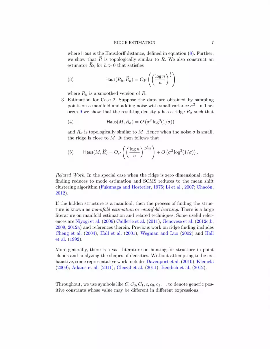
Figure 3. The Mean Shift Algorithm. The data points move along trajectories duringiterations until they reach the two modes marked by the two large asterisks.

The mean shift algorithm (Fukunaga and Hostetler (1975); Comaniciu andMeer (2002)) is a method for finding the modes of a density by following thesteepest ascent paths. The algorithm starts with a mesh of points and thenmoves the points along gradient ascent trajectories towards local maxima.We describe the method in Section 7. A simple example is shown in Figure 3.Mode finding is similar to level set estimation (Polonik, 1995; Cadre, 2006;Walther, 1997) but in general, the two problems are not the same.

Overview of the Results. Here we give a non-technical description of themain results. A ridge R of a density function p is a low dimensional set(such as a curve in two dimensions) where the density is sharply peaked inone direction and smooth in the perpendicular direction as in Figure 4.

1. Stability. In Theorem 6 we give a stability theorem for ridges. We showthat if two functions are sufficiently close together then their ridges arealso close together.

2. Estimation for Case 1. In Theorem 7 we show that there is an estimatorR such that

(2) Haus(R, R) = OP

((log n

n

) 2D+8

)

RIDGE ESTIMATION 7

where Haus is the Hausdorff distance, defined in equation (8). Further,we show that R is topologically similar to R. We also construct anestimator Rh for h > 0 that satisfies

(3) Haus(Rh, Rh) = OP

((log n

n

) 12

)where Rh is a smoothed version of R.

3. Estimation for Case 2. Suppose the data are obtained by samplingpoints on a manifold and adding noise with small variance σ2. In The-orem 9 we show that the resulting density p has a ridge Rσ such that

(4) Haus(M,Rσ) = O(σ2 log3(1/σ)

)and Rσ is topologically similar to M . Hence when the noise σ is small,the ridge is close to M . It then follows that

(5) Haus(M, R) = OP

((log n

n

) 2D+8

)+O

(σ2 log3(1/σ)

).

Related Work. In the special case when the ridge is zero dimensional, ridgefinding reduces to mode estimation and SCMS reduces to the mean shiftclustering algorithm (Fukunaga and Hostetler, 1975; Li et al., 2007; Chacon,2012).

If the hidden structure is a manifold, then the process of finding the struc-ture is known as manifold estimation or manifold learning. There is a largeliterature on manifold estimation and related techniques. Some useful refer-ences are Niyogi et al. (2006) Caillerie et al. (2011), Genovese et al. (2012c,b,2009, 2012a) and references therein. Previous work on ridge finding includesCheng et al. (2004), Hall et al. (2001), Wegman and Luo (2002) and Hallet al. (1992).

More generally, there is a vast literature on hunting for structure in pointclouds and analyzing the shapes of densities. Without attempting to be ex-haustive, some representative work includes Davenport et al. (2010); Klemela(2009); Adams et al. (2011); Chazal et al. (2011); Bendich et al. (2012).

Throughout, we use symbols like C,C0, C1, c, c0, c1 . . . to denote generic pos-itive constants whose value may be different in different expressions.


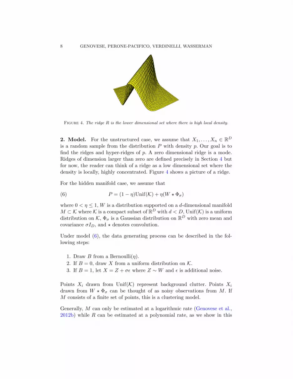
Figure 4. The ridge R is the lower dimensional set where there is high local density.

2. Model. For the unstructured case, we assume that X1, . . . , Xn ∈ RDis a random sample from the distribution P with density p. Our goal is tofind the ridges and hyper-ridges of p. A zero dimensional ridge is a mode.Ridges of dimension larger than zero are defined precisely in Section 4 butfor now, the reader can think of a ridge as a low dimensional set where thedensity is locally, highly concentrated. Figure 4 shows a picture of a ridge.

For the hidden manifold case, we assume that

(6) P = (1− η)Unif(K) + η(W ? Φσ)

where 0 < η ≤ 1, W is a distribution supported on a d-dimensional manifoldM ⊂ K where K is a compact subset of RD with d < D, Unif(K) is a uniformdistribution on K, Φσ is a Gaussian distribution on RD with zero mean andcovariance σID, and ? denotes convolution.

Under model (6), the data generating process can be described in the fol-lowing steps:

1. Draw B from a Bernoulli(η).

2. If B = 0, draw X from a uniform distribution on K.

3. If B = 1, let X = Z + σε where Z ∼W and ε is additional noise.

Points Xi drawn from Unif(K) represent background clutter. Points Xi

drawn from W ? Φσ can be thought of as noisy observations from M . IfM consists of a finite set of points, this is a clustering model.

Generally, M can only be estimated at a logarithmic rate (Genovese et al.,2012b) while R can be estimated at a polynomial rate, as we show in this

RIDGE ESTIMATION 9

M R

Rh

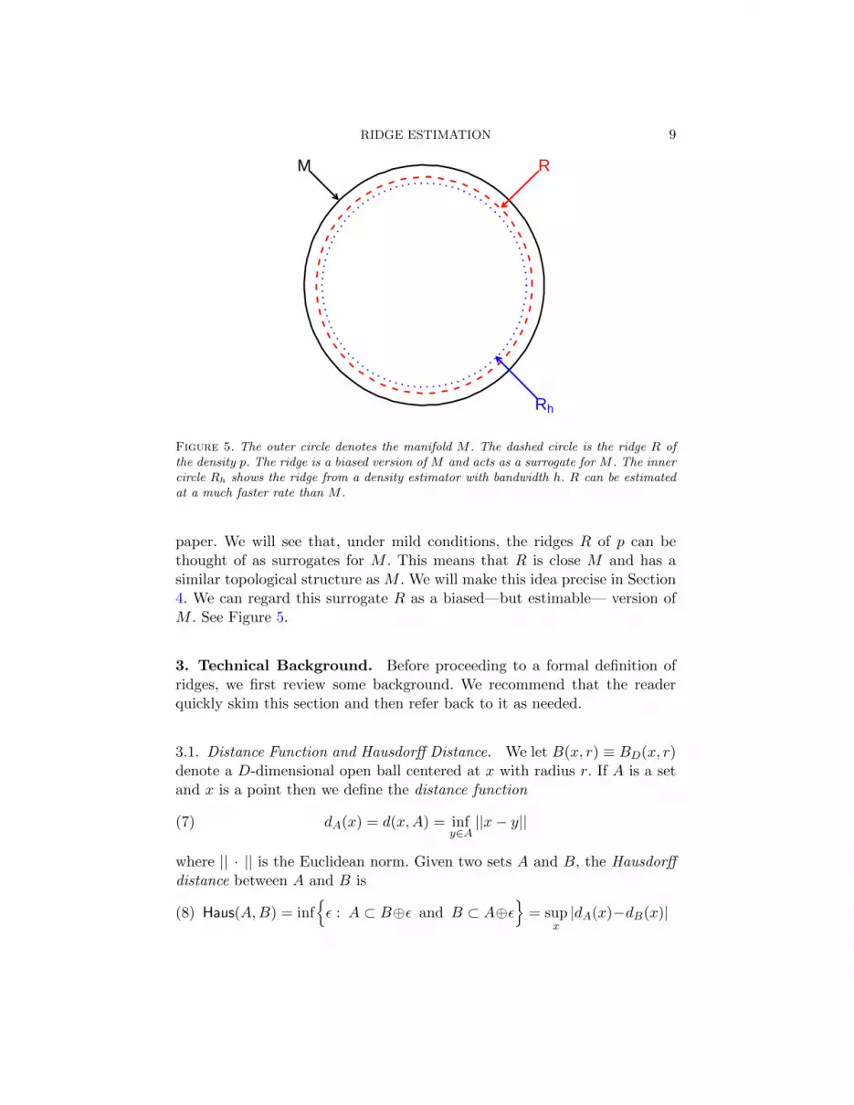
Figure 5. The outer circle denotes the manifold M . The dashed circle is the ridge R ofthe density p. The ridge is a biased version of M and acts as a surrogate for M . The innercircle Rh shows the ridge from a density estimator with bandwidth h. R can be estimatedat a much faster rate than M .

paper. We will see that, under mild conditions, the ridges R of p can bethought of as surrogates for M . This means that R is close M and has asimilar topological structure as M . We will make this idea precise in Section4. We can regard this surrogate R as a biased—but estimable— version ofM . See Figure 5.

3. Technical Background. Before proceeding to a formal definition ofridges, we first review some background. We recommend that the readerquickly skim this section and then refer back to it as needed.

3.1. Distance Function and Hausdorff Distance. We let B(x, r) ≡ BD(x, r)denote a D-dimensional open ball centered at x with radius r. If A is a setand x is a point then we define the distance function

(7) dA(x) = d(x,A) = infy∈A||x− y||

where || · || is the Euclidean norm. Given two sets A and B, the Hausdorffdistance between A and B is

(8) Haus(A,B) = inf{ε : A ⊂ B⊕ε and B ⊂ A⊕ε

}= sup

x|dA(x)−dB(x)|


where

(9) A⊕ ε =⋃x∈A

BD(x, ε) ={x : dA(x) ≤ ε

}is called the ε-offset of A. The offset can be thought of as a smoothed versionof A. For example, if there are any small holes in A, these will be filled inby forming the offset A⊕ ε.

We use Hausdorff distance to measure the distance between sets for severalreasons: it is the most commonly used distance between sets, it is a very strictdistance and is analogous to the familiar L∞ distance between functions forsets.

3.2. Topological Concepts. This subsection follows Chazal, Cohen-Steinerand Lieutier (2009) Chazal et al. (2009) and Chazal and Lieutier (2005).The reach of a set K, denoted by reach(K), is the largest r > 0 such thateach point in K ⊕ r has a unique projection onto K. A set with positivereach is, in a sense, a smooth set without self-intersections.

Now we describe a generalization of reach called µ-reach. The key pointis simply that the µ-reach is weaker than reach. The full details can befound in the aforementioned references. Let A be a compact set. FollowingChazal and Lieutier (2005) define the gradient ∇A(x) of dA(x) to be theusual gradient function whenever this is well defined. However, there maybe points x at which dA is not differentiable in the usual sense. In that case,define the gradient as follows. For x ∈ A define ∇A(x) = 0 for all x ∈ A.For x /∈ A, let Γ(x) = {y ∈ A : ||x − y|| = dA(x)}. Let Θ(x) be the centerof the unique smallest closed ball containing Γ(x). Define

(10) ∇A(x) =x−Θ(x)

dA(x).

The critical points are the points at which ∇A(x) = 0. The weak feature sizewfs(A) is the distance from A to its closest critical point. For 0 < µ < 1, theµ-reach reachµ(A) is

(11) reachµ(A) = inf{d : χ(d) < µ}

where χ(d) = inf{||∇A(x)|| : dA(x) = d}. It can be shown that reachµ isnon-increasing in µ, that wfs(A) = limµ→0 reachµ(A) and that reach(A) =limµ→1 reachµ(A).

RIDGE ESTIMATION 11

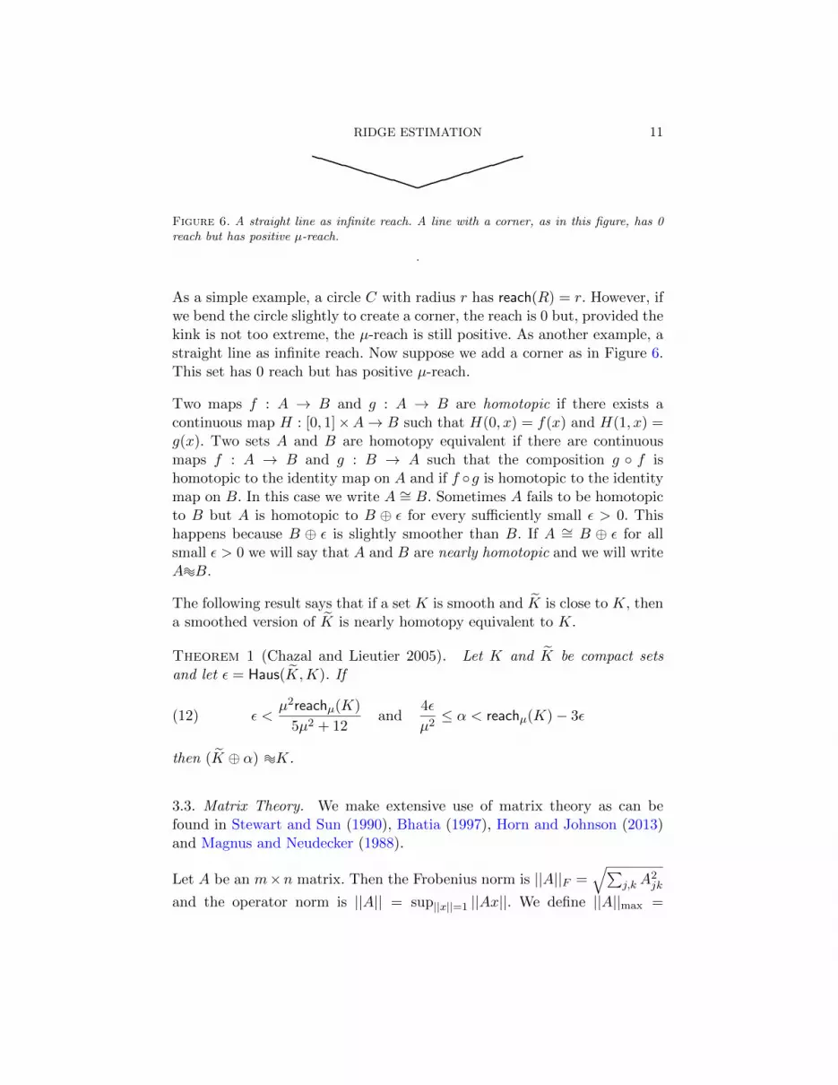
Figure 6. A straight line as infinite reach. A line with a corner, as in this figure, has 0reach but has positive µ-reach.

.

As a simple example, a circle C with radius r has reach(R) = r. However, ifwe bend the circle slightly to create a corner, the reach is 0 but, provided thekink is not too extreme, the µ-reach is still positive. As another example, astraight line as infinite reach. Now suppose we add a corner as in Figure 6.This set has 0 reach but has positive µ-reach.

Two maps f : A → B and g : A → B are homotopic if there exists acontinuous map H : [0, 1]×A→ B such that H(0, x) = f(x) and H(1, x) =g(x). Two sets A and B are homotopy equivalent if there are continuousmaps f : A → B and g : B → A such that the composition g ◦ f ishomotopic to the identity map on A and if f ◦g is homotopic to the identitymap on B. In this case we write A ∼= B. Sometimes A fails to be homotopicto B but A is homotopic to B ⊕ ε for every sufficiently small ε > 0. Thishappens because B ⊕ ε is slightly smoother than B. If A ∼= B ⊕ ε for allsmall ε > 0 we will say that A and B are nearly homotopic and we will writeA@B.

The following result says that if a set K is smooth and K is close to K, thena smoothed version of K is nearly homotopy equivalent to K.

Theorem 1 (Chazal and Lieutier 2005). Let K and K be compact setsand let ε = Haus(K,K). If

(12) ε <µ2reachµ(K)

5µ2 + 12and

4ε

µ2≤ α < reachµ(K)− 3ε

then (K ⊕ α) @K.

3.3. Matrix Theory. We make extensive use of matrix theory as can befound in Stewart and Sun (1990), Bhatia (1997), Horn and Johnson (2013)and Magnus and Neudecker (1988).

Let A be an m×n matrix. Then the Frobenius norm is ||A||F =√∑

j,k A2jk

and the operator norm is ||A|| = sup||x||=1 ||Ax||. We define ||A||max =


maxj,k |Ajk|. It is well known that ||A|| ≤ ||A||F ≤√n||A||, that ||A||max ≤

||A|| ≤√mn||A||max and that ||A||F ≤

√mn||A||max.

The vec operator converts a matrix into a vector by stacking the columns.Thus, if A is m×n then vec(A) is a vector of length mn. Conversely, given avector a of length mn, let [[a]] denote the m×n matrix obtained by stackinga columnwise into matrix form.

If A is m×n and B is p×q then the Kronecker A⊗B is the mp×nq matrix

(13)

A11B · · · A1nB...

...Am1B · · · AmnB

.If A and B have the same dimensions, then the Hadamard product C = A◦Bis defined by Cjk = AjkBjk.

For matrix calculus, we follow the conventions in Magnus and Neudecker(1988). If F : RD → Rk is a vector-valued map then the Jacobian matrixwill be denoted by F ′(x) or dF/dx. This is the D×k matrix with F ′(x)jk =∂Fi(x)/∂xj . If F : RD → Rm×p is a matrix-valued map then F ′(x) is amp×D matrix defined by

(14) F ′(x) ≡ dF

dx=dvec(F (x))

dx.

If F : Rn×q → Rm×p then the derivative is a mp× nq matrix given by

F ′(X) ≡ dF

dX=dvec(F (X))

dvec(X).

We then have the following product rule for matrix calculus: if F : RD →Rm×p and G : RD → Rp×q then

dF (x)G(x)

dx= (GT (x)⊗ Im)F ′(x) + (Iq ⊗ F (x))G′(x).

Also, if A(x) = f(x)I then A′(x) = vec(I) ⊗ (∇f(x))T where ∇f denotesthe gradient of f .

Now we consider a special class of matrix valued functions: symmetric spec-tral functions (also called primary matrix functions); see section V.3 of Bha-tia (1997) and Chen et al. (2003). Let S be the set of symmetric D × Dmatrices. Let f : R → R. Let H ∈ S have spectral decomposition H =

RIDGE ESTIMATION 13

UΛUT where Λ = diag(λ1, . . . , λD) with λ1 ≥ λ2 ≥ · · · ≥ λD. Define amatrix function f� by

(15) f�(H) = U

f(λ1) 0 · · · 0

0 f(λ2) · · · 0...

.... . .

...0 0 · · · f(λD)

UT .The function f� : S → S is well-defined. It does not depend on the orderingof the eigenvalues or the choice of U in case of multiplicities of the eigen-values (Bhatia, 1997). Also, f� is continuously differentiable if and only iff is continuously differentiable. In general, f� inherits whatever smooth-ness conditions (continuity, differentiability, etc) that f has; see Chen et al.(2003).

We say that f� is Frechet differentiable if there exists a linear map f †�(H)such that

(16) f�(H + E)− f�(H)− f †�(H)E = o(||E||F ).

The Frechet derivative f †�(H) is given by (Bhatia (1997))

(17) f †�(H)E = U(f∗ ◦ (UTEU)

)UT for all E ∈ S

where ◦ denotes the Hadamard product and f∗ is a D × D matrix withentries

(18) f∗ij =

f(λi)−f(λj)

λi−λj if λi 6= λj

f ′(λi) if λi = λj .

The following version of the Davis-Kahan Theorem is from Von Luxburg(2007). Let H and H be two symmetric, square D ×D matrices. Let Λ bethe eigenvalues of H. Let S ⊂ R and let V (V ) be the matrix whose columnsare the eigenvectors corresponding to the eigenvalues of H (H) in S. Let

(19) β = min{|λ− s| : λ ∈ Λ

⋂Sc, s ∈ S

}.

According to the Davis-Kahan theorem,

(20) ||V V T − V V T || ≤ ||H − H||Fβ

.


Let H be a D×D square, symmetric matrix with eigenvalues λ1 ≥ · · · ≥ λD.Let H be another square, symmetric matrix with eigenvalues λ1 ≥ · · · ≥ λD.By Weyl’s theorem (Theorem 4.3.1 of Horn and Johnson (2013)) we havethat

(21) λn(H −H) + λi(H) ≤ λi(H) ≤ λi(H) + λ1(H −H).

It follows easily that

(22) |λi(H)− λi(H)| ≤ ||H − H|| ≤ D ||H − H||max.

4. Ridges. In this section we provide a mathematical framework for ridges.Specifically, we do the following:

1. We give a formal definition for ridges.

2. We establish some basic properties of ridges.

3. We show that, under appropriate conditions, if two functions are closetogether then their ridges are close and their ridges are topologicallysimilar.

As in Ozertem and Erdogmus (2011), our definition of ridges relies on thegradient and Hessian of the density function p.

4.1. Definitions. Given a function p : RD → R, let g(x) = ∇p(x) denotethe gradient at x and let H(x) denote the Hessian matrix. Let

(23) λ1(x) ≥ λ2(x) ≥ · · · ≥ λD(x)

denote the eigenvalues of H(x) and let Λ(x) be the diagonal matrix whosediagonal elements are the eigenvalues. Write the spectral decomposition ofH(x) as H(x) = U(x)Λ(x)U(x)T . Fix 0 ≤ d < D and let V (x) be the lastD − d columns of U(x) (that is, the columns corresponding to the D − dsmallest eigenvalues). If we write U(x) = [V�(x) : V (x)] then we can writeH(x) = [V�(x) : V (x)]Λ(x)[V�(x) : V (x)]T . Let L(x) = V (x)V (x)T be theprojector on the linear space defined by the columns of V (x). Define theprojected gradient

(24) G(x) = L(x)g(x).

If the vector field G(x) is Lipschitz then by Theorem 3.39 of Irwin (1980),G defines a global flow as follows. The flow is a family of functions φ(x, t)

RIDGE ESTIMATION 15

such that φ(x, 0) = x and φ′(x, 0) = G(x) and φ(s, φ(t, x)) = φ(s+t, x). Theflow lines, or integral curves, partition the space and at each x where G(x)is non-null, there is a unique integral curve passing through x. The intuitionis that the flow passing through x is a gradient ascent path moving towardshigher values of p. Unlike the paths defined by the gradient g which movetowards modes, the paths define by G move towards ridges.

The paths can be parameterized in many ways. One commonly used para-meterization is to use t ∈ [−∞,∞] where large values of t correspond tohigher values of p. In this case t = ∞ will correspond to a point on theridge. In this parameterization we can express each integral curve in theflow as follows. A map π : R→ RD is an integral curve with respect to theflow of G if

(25) π′(t) = G(π(t)) = L(π(t))g(π(t)).

Definition: The ridge R consists of the destinations of the integral curves:y ∈ R if limt→∞ π(t) = y for some π satisfying (25).

As mentioned above, the integral curves partition the space and for eachx /∈ R, there is a unique path πx passing through x. The ridge points arezeros of the projected gradient: y ∈ R implies that G(y) = (0, . . . , 0)T .

It will also be convenient to parameterize the curves by arclength. Thus, lets ≡ s(t) be the arclength from π(t) to π(∞):

(26) s(t) =

∫ ∞t||π′(u)||du.

Let t ≡ t(s) denote the inverse of s(t). Note that

(27) t′(s) = − 1

||π′(t(s))||= − 1

||L(π(t(s)))g(π(t(s)))||= − 1

||G(π(t(s)))||.

Let γ(s) = π(t(s)). Then

(28) γ′(s) = − G(γ(s))

||G(γ(s))||

which is a restatement of (25) in the arclength parameterization.

In what follows, we will often abbreviate notation by using the subscript sin the following way: Gs = G(γ(s)), Hs = H(γ(s)), . . ., etc.


4.2. Differentials. We will need derivatives of g, H, and L. The derivativeof g is the Hessian H. Recall from (14) that H ′(x) = dvec(H(x))

dx . We alsoneed derivatives along the curve γ. The derivative of a functions f along γis

(29).fγ(s) ≡

.fs = lim

ε→0

f(γ(s+ ε))− f(γ(s))

ε.

Thus, the derivative of the gradient g along γ is

(30).gγ(s) ≡

.gs = lim

ε→0

g(γ(s+ ε))− g(γ(s))

ε= Hsγ

′s = −HsGs

||Gs||.

We will also need the derivative of H in the direction of a vector z whichwe will denote by

H ′(x; z) ≡ limε→0

H(x+ εz)−H(x)

ε.

We can write an explicitly formula for H ′(x; z) as follows. Note that theelements of H ′ are simply the partial derivatives ∂Hjk(x)/∂x` arranged ina D2 × D matrix. Hence, H ′(x; z) = [[H ′(x)z]]. (Recall that [[a]] stacks avector into a matrix.)

The collection {L(x) : x ∈ RD} defines a matrix field: there is a matrixL(x) attached to each point x. We will need the derivative of this field alongthe integral curves γ. For any x /∈ R, there is a unique path γ and uniques > 0 such that x = γ(s). Define

(31).Ls ≡

.L(x) ≡ lim

ε→0

L(H(γ(s+ ε)))− L(H(γ(s)))

ε.

To compute the direction derivative.Ls, we first need the Frechet derivative

L† of L when L = L(H) is viewed as a map L : S → S where S is the setof symmetric D×D matrices. Let b1 < b2 be real numbers with b1 < 0 andβ ≡ b2 − b1 > 0. Let Sβ denote all D × D symmetric matrices such thatλj ≥ b2 for j = 1, . . . , d and λj ≤ b1 for j = d+ 1, . . . , D.

Lemma 2. The Frechet derivative L† of L on Sβ satisfies,

(32) L†E = U

([0d −B−BT 0D−d

]◦ (UTEU)

)UT for each E ∈ S,

RIDGE ESTIMATION 17

where 0k denotes a k × k matrix of zeroes, B is a d × (D − d) matrix withentries

(33) Bjk =1

λj(x)− λd+k(x), 1 ≤ j ≤ d, 1 ≤ k ≤ D − d.

Proof. For H ∈ Sβ with H = UΛUT write U = [V� : V ] and let L =L(H) = V V T which is the projector onto to the space spanned by theeigenvectors corresponding to λd+1, . . . , λD.

Now take f to be any monotone, differentiable function such that f(x) = 1for x ≤ b1 and f(x) = 0 for x ≥ b2. It follows that, for each H ∈ Sβ,L(H) = f�(H). Then

(34) f∗ =

[0 −B−BT 0

]where f∗ was defined in (18). Hence, from (17), for all E ∈ S,

(35) L†E = U

([0 −B−BT 0

]◦ (UTEU)

)UT .

Now we can find.Ls. Recall that H ′(x; z) = [[H ′z]] denotes the direction

derivative of H in the direction z.

Theorem 3. Let x = γ(s) and write H = Hs = UΛUT and H ′ = H ′(x).Suppose that H(y) ∈ Sβ for all y in an open neighborhood around x. Wehave that

(36).Ls(x) =

1

||Gs||U

([0d×d −B−BT 0(D−d)×(D−d)

]◦ (UT [[H ′Gs]]U)

)UT .

Proof. Recall that γ′s = −Gs/||Gs||. Let E = [[H ′γ′s]] = −[[H ′Gs]]/||Gs||.Note that

γ(s+ ε) = γ(s) + εγ′(s) + o(ε) = γ(s)− εGs/||Gs||+ o(ε)

and

Hs+ε = H(γ(s) + εγ′(s)) + o(ε)) = H + εH ′(γ(s); γ′(s)) + o(ε)

= H + ε[[H ′γ′(s)]] + o(ε) = H + εE + o(ε).


Hence,

.Ls = lim

ε→0

L(H(γ(s+ ε)))− L(H(γ(s)))

ε= lim

ε→0

L(H + εE)− L(H)

ε= L†E

where L† is the Frechet derivative of L. As we showed earlier, the Frechetderivative L†, satisfies the following equation for any E ∈ S,

L†E = U

([0 −B−BT 0

]◦ (UTEU)

)UT .

Hence, with E = −[[H ′Gs]]/||Gs||,

.Ls = L†E =

1

||Gs||U

([0 −B−BT 0

]◦ (UT [[H ′Gs]]U)

)UT .

4.3. Assumptions. We now record the main assumptions that we will re-quire for the results.

Assumption (A0). For all x, g(x), H(x) and H ′(x) exist.

Assumption (A1). There exists β > 0, δ > 0 and b1 < b2 such that,b1 < 0, β = b2 − b1, and for all x ∈ R⊕ δ,

λj(x) > b2, j = 1, . . . , d and λj(x) < b1, j = d+ 1, . . . , D.(A1)

Assumption (A2). For each x ∈ R⊕ δ,

||g(x)|| ||H ′(x)||max <β2

2√D.(A2)

Condition (A1) says that p is sharply curved around the ridge in the D− ddimensional space normal to the ridge. It is akin to requiring a functionto have a negative second derivative at a mode. (A2) is a third derivativecondition which implies that the paths cannot be too wiggly.

Lemma 4. Conditions (A0)-(A2) imply that, for each x ∈ (R ⊕ δ) − R,there is a unique path γ passing through x.

RIDGE ESTIMATION 19

Proof. We will show that the vector field G(x) is Lipschitz over R⊕δ. Theresult then follows from Theorem 3.39 of Irwin (1980). Recall that G = Lgand g is differentiable. It suffices to show that L is differentiable over R⊕ δ.Now L(x) = L(H(x)). The Frechet derivative of L as a function of H wasgiven in Lemma 2. And H is differentiable by assumption. By the chain rule,L is differentiable as a function of x. Indeed, dL/dx is the D2 ×D matrixwhose jth column is vec(L†Ej) where Ej = [[H ′ej ]] and ej is the vectorwhich is 1 in the jth coordinate and zero otherwise.

4.4. Quadratic Behavior. Conditions (A1) and (A2) imply that the func-tion p has quadratic-like behavior near the ridges. This property is neededfor establishing the convergence of ridge estimators. In this section we form-alize this notion of quadratic behavior. Give a path γ, define the function

(37) ξ(s) = p(π(∞))− p(π(t(s))) = p(γ(0))− p(γ(s)).

Thus ξ is simply the drop in the function p along the curve γ as we move awayfrom the ridge. We write ξx(s) if we want to emphasize that ξ correspondsto the path γx passing through the point x. Since ξ : [0,∞) → [0,∞), wedefine its derivatives in the usual way, i.e. ξ′(s) = dξ(s)/ds.

Lemma 5. Suppose that (A0)-(A2) hold. For all x ∈ R ⊕ δ, the followingare true:

1. ξ(0) = 0.

2. ξ′(s) = ||G(γ(s))|| and ξ′(0) = 0.

3. The second derivative of ξ is:

(38) ξ′′(s) = −GTsHsGs||Gs||2

+gTs

.LsGs||Gs||

.

4. ξ′′(s) ≥ β/2.

5. ξ(s) is non-increasing in s.

6. ξ(s) ≥ β4 ||γ(0)− γ(s)||2.

Proof. 1. The first condition ξ(0) = 0 is immediate from the definition.


2. Next,

ξ′(s) = −dp(γ(s))

ds= −gsγ′s =

gTs Gs||Gs||

=gTs Lsgs||Gs||

=gTs LsLsgs||Gs||

=GTs Gs||Gs||

= ||Gs||.

Since the projected gradient is 0 at the ridge, we have that ξ′(0) = 0.

3. Note that (ξ′(s))2 = ||Gs||2 = GTs Gs = gTs Lsgs ≡ a(s). Differentiatingboth sides of this equation we have that 2ξ′(s)ξ′′(s) = a′(s) and hence

ξ′′(s) =a′(s)

2ξ′(s)=

a′(s)

2||Gs||.

Now

(39) a′(s) = (.gs)

TLsgs + gTs.Lsgs + gTs Ls

.gs = 2(

.gs)

TLsgs + gTs.Lsgs.

Since LsLs = Ls we have that.Ls = Ls

.Ls +

.LsLs and hence

gTs.Lsgs = gTs Ls

.Lsgs + gTs

.LsLsgs = GTs

.Lsgs + gTs

.LsGs = 2gTs

.LsGs.

Therefore,

(40) a′(s) = 2(.gs)

TLsgs + 2gTs.LsGs.

Recall that.gs = −HsGs

||Gs|| . Thus,

(41) ξ′′(s) =a′(s)

2||Gs||= −G

TsHsGs||Gs||2

+gTs

.LsGs||Gs||

.

4. The first term in ξ′′(s) is −GTs HsGs||Gs||2 . Since G is in the column space of

V , GTsHsGs = GTs (VsΛsVTs )Gs where Λs = diag(λd+1(γ(s)), . . . , λD(γ(s))).

Hence, from (A1),

GTsHsGs||Gs||2

=GTs (VsΛsV

Ts )Gs

||Gs||2≤ λmax(VsΛsV

Ts ) ≤ −β

and thus

−GTsHsGs||Gs||2

≥ β.

RIDGE ESTIMATION 21

Now we bound the second term. The second term is

gTs.LsGs||Gs||

=1

||Gs||2gTs

{U


]◦ (UT [[H ′Gs]]U)

)UT

}Gs

= gTs

{U


]◦ (UT [[H ′As]]U)

)UT

}As

where As = Gs/||Gs||. As is a unit vector in the column space of V . Now,the || · ||max||-norm of the term inside the braces {·} is bounded above by√D||H ′||max/β. Here we used the fact that, due to (A1), |Bjk| ≤ 1/β for

each j, k. Hence, from (A2),

|gTs.LsGs|||Gs||

≤√D||H ′||max |gTs As|

β≤√D||H ′||max ||gs||

β≤ β

2.

5. Follows from 2.

6. For some 0 ≤ s ≤ s,

ξ(s) = ξ(0) + sξ′(0) +s2

2ξ′′(s) =

s2

2ξ′′(s) ≥ βs2

4

from part (4). So

ξ(s)− ξ(0) ≥ β

4s2 ≥ β

4||γ(0)− γ(s)||2.

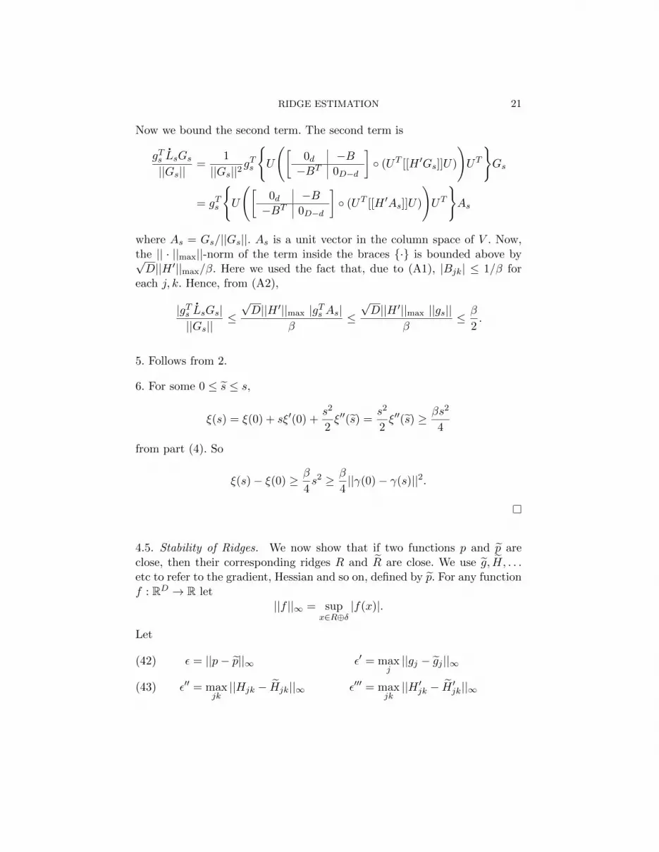
4.5. Stability of Ridges. We now show that if two functions p and p areclose, then their corresponding ridges R and R are close. We use g, H, . . .etc to refer to the gradient, Hessian and so on, defined by p. For any functionf : RD → R let

||f ||∞ = supx∈R⊕δ

|f(x)|.

Let

ε = ||p− p||∞ ε′ = maxj||gj − gj ||∞(42)

ε′′ = maxjk||Hjk − Hjk||∞ ε′′′ = max

jk||H ′jk − H ′jk||∞(43)


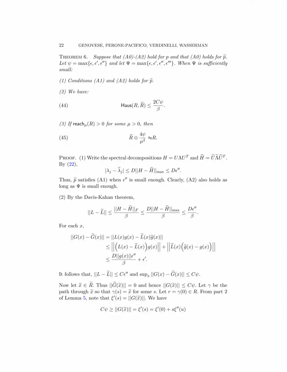
Theorem 6. Suppose that (A0)-(A2) hold for p and that (A0) holds for p.Let ψ = max{ε, ε′, ε′′} and let Ψ = max{ε, ε′, ε′′, ε′′′}. When Ψ is sufficientlysmall:

(1) Conditions (A1) and (A2) holds for p.

(2) We have:

(44) Haus(R, R) ≤ 2Cψ

β.

(3) If reachµ(R) > 0 for some µ > 0, then

(45) R⊕ 4ψ

µ2@R.

Proof. (1) Write the spectral decompositionsH = UΛUT and H = U ΛUT .By (22),

|λj − λj | ≤ D||H − H||max ≤ Dε′′.

Thus, p satisfies (A1) when ε′′ is small enough. Clearly, (A2) also holds aslong as Ψ is small enough.

(2) By the Davis-Kahan theorem,

||L− L|| ≤ ||H − H||Fβ

≤ D||H − H||max

β≤ Dε′′

β.

For each x,

||G(x)− G(x)|| = ||L(x)g(x)− L(x)g(x)||

≤∣∣∣∣∣∣(L(x)− L(x)

)g(x)

∣∣∣∣∣∣+∣∣∣∣∣∣L(x)

(g(x)− g(x)

)∣∣∣∣∣∣≤ D||g(x)||ε′′

β+ ε′.

It follows that, ||L− L|| ≤ Cε′′ and supx ||G(x)− G(x)|| ≤ Cψ.

Now let x ∈ R. Thus ||G(x)|| = 0 and hence ||G(x)|| ≤ Cψ. Let γ be thepath through x so that γ(s) = x for some s. Let r = γ(0) ∈ R. From part 2of Lemma 5, note that ξ′(s) = ||G(x)||. We have

Cψ ≥ ||G(x)|| = ξ′(s) = ξ′(0) + sξ′′(u)

RIDGE ESTIMATION 23

for some u between s and 0. Since ξ′(0) = 0, from part 4 of Lemma 5,

Cψ ≥ sξ′′(u) ≥ sβ

2

and so

||r − x|| ≤ s ≤ 2Cψ

β.

Thus, d(x, R) ≤ ||r − x|| ≤ 2Cψ/β.

Now let x ∈ R. The same argument shows that d(x, R) ≤ 2Cψ/β since (A1)and (A2) hold for p.

(3) Choose any fixed κ > 0 such that κ < µ2

5µ2+12. When Ψ is sufficiently

small, Ψ ≤ κ reachµ(K). Then R⊕ 4ψµ2

@R from Theorem 1.

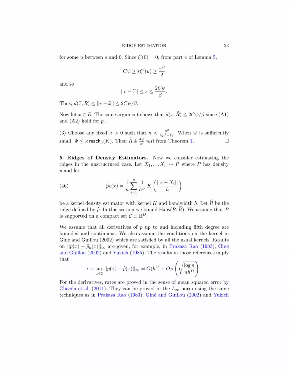
5. Ridges of Density Estimators. Now we consider estimating theridges in the unstructured case. Let X1, . . . Xn ∼ P where P has densityp and let

(46) ph(x) =1

n

n∑i=1

1

hDK

(||x−Xi||

h

)

be a kernel density estimator with kernel K and bandwidth h. Let R be theridge defined by p. In this section we bound Haus(R, R). We assume that Pis supported on a compact set C ⊂ RD.

We assume that all derivatives of p up to and including fifth degree arebounded and continuous. We also assume the conditions on the kernel inGine and Guillou (2002) which are satisfied by all the usual kernels. Resultson ||p(x) − ph(x)||∞ are given, for example, in Prakasa Rao (1983), Gineand Guillou (2002) and Yukich (1985). The results in those references implythat

ε ≡ supx∈C||p(x)− p(x)||∞ = O(h2) +OP

(√log n

nhD

).

For the derivatives, rates are proved in the sense of mean squared error byChacon et al. (2011). They can be proved in the L∞ norm using the sametechniques as in Prakasa Rao (1983), Gine and Guillou (2002) and Yukich


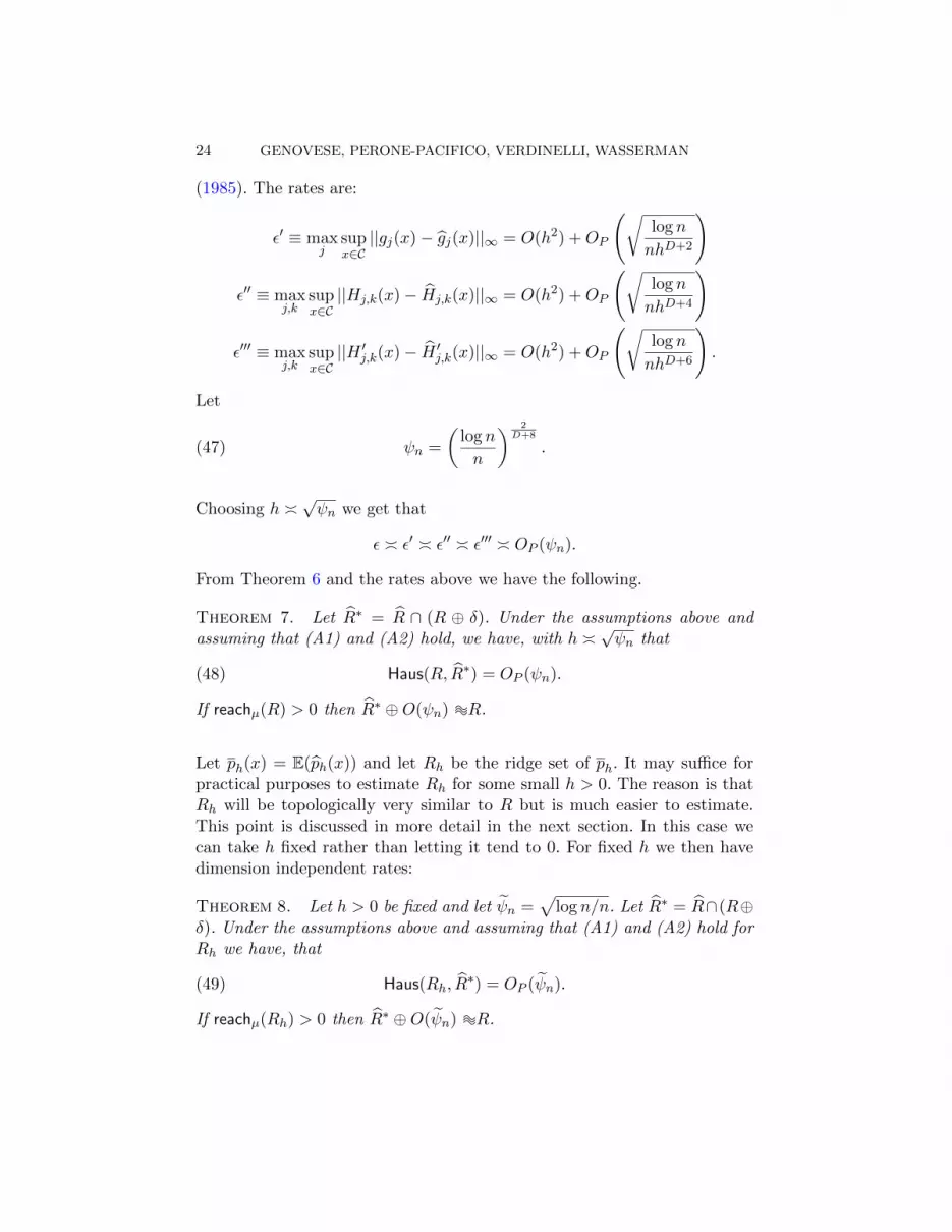
(1985). The rates are:

ε′ ≡ maxj

supx∈C||gj(x)− gj(x)||∞ = O(h2) +OP

(√log n

nhD+2

)

ε′′ ≡ maxj,k

supx∈C||Hj,k(x)− Hj,k(x)||∞ = O(h2) +OP

(√log n

nhD+4

)

ε′′′ ≡ maxj,k

supx∈C||H ′j,k(x)− H ′j,k(x)||∞ = O(h2) +OP

(√log n

nhD+6

).

Let

(47) ψn =

(log n

n

) 2D+8

.

Choosing h �√ψn we get that

ε � ε′ � ε′′ � ε′′′ � OP (ψn).

From Theorem 6 and the rates above we have the following.

Theorem 7. Let R∗ = R ∩ (R ⊕ δ). Under the assumptions above andassuming that (A1) and (A2) hold, we have, with h �

√ψn that

(48) Haus(R, R∗) = OP (ψn).

If reachµ(R) > 0 then R∗ ⊕O(ψn) @R.

Let ph(x) = E(ph(x)) and let Rh be the ridge set of ph. It may suffice forpractical purposes to estimate Rh for some small h > 0. The reason is thatRh will be topologically very similar to R but is much easier to estimate.This point is discussed in more detail in the next section. In this case wecan take h fixed rather than letting it tend to 0. For fixed h we then havedimension independent rates:

Theorem 8. Let h > 0 be fixed and let ψn =√

log n/n. Let R∗ = R∩(R⊕δ). Under the assumptions above and assuming that (A1) and (A2) hold forRh we have, that

(49) Haus(Rh, R∗) = OP (ψn).

If reachµ(Rh) > 0 then R∗ ⊕O(ψn) @R.

RIDGE ESTIMATION 25

6. Ridges as Surrogates for Hidden Manifolds. Consider now thecase where Pσ = (1 − η)Unif(K) + η(W ? Φσ) where W is supported onM . We assume that W has a twice-differentiable density w respect to theuniform measure on M . We also assume that w is bounded away from zeroand ∞.

We want to show that the ridge of pσ is a surrogate for M . Specifically weshow that, as σ gets small, there is a subset R∗ ⊂ R in a neighborhoodof M such that Haus(M,R∗) = O(σ2 log3(1/σ)) and such that R∗ @M .We assume that η = 1 in what follows; the extension to 0 < η < 1 isstraightforward. We assume that M is a compact d-manifold with positivereach κ. We need to assume that M has positive reach rather than justpositive µ-reach. The reason is that, when M has positive reach, the measureW induces a smooth distribution on the tangent space TxM for each x ∈M .We need this property in our proofs and this property is lost if M only haspositive µ-reach for some µ < 1 due to the presence of unsmooth featuressuch as corners.

The density of X is

(50) pσ(x) =

∫Mφσ(x− z)dW (z)

where φσ(u) = (2π)−D/2σ−D exp(− ||u||

2

2σ2

). Thus, pσ is a mixture of Gaus-

sians. However, it is a rather unusual mixture; it is a singular mixture ofGaussians since the mixing distribution W is supported on a lower dimen-sional manifold.

Let TxM be the tangent space to M at x and let T⊥x M be the normalspace to M at x. Define the fiber at x ∈ M by Fx = T⊥x M ∩ BD(x, r). Aconsequence of the fact that the reach κ is positive is that, for any 0 < r < κ,M ⊕ r can be written as a disjoint union

(51) M ⊕ r =⋃x∈M

Fx.

Let rσ > 0 satisfy the following conditions:

(52) rσ < σ,rσσ2→∞, rσ log

(1

σ2+D

)= o(1) as σ → 0.

Specifically, take rσ = ασ for some 0 < α < 1. Fix any A ≥ 2 and define

(53) Kσ =

√2σ2 log

(1

σA+D

).


Theorem 9 (Surrogate Theorem). Suppose that κ = reach(M) > 0.Let Rσ be the ridge set of pσ. Let Mσ = M ⊕ rσ and R∗σ = Rσ

⋂Mσ. For

all small σ > 0:

1. R∗σ satisfies (A1) and (A2) with β = c σ−(D−d+2) form some c > 0.

2. Haus(M,R∗σ) = O(K2σ).

3. R∗σ ⊕ CK2σ @M .

If Rσ is instead taken to be the ridge set of log pσ then the same results aretrue with β = cσ−2 and Mσ = M ⊕ κ.

The theorem shows that in a neighborhood of the manifold, there is a well-defined ridge, that the ridge is close to the manifold and is nearly homo-topic to the manifold. It is interesting to compare the above result to recentwork on finite mixtures of Gaussians (Carreira-Perpinan and Williams, 2003;Edelsbrunner et al., 2012). In those papers, it is shown that there can befewer or more modes than the number of Gaussian components in a finitemixture. However, for small σ, it is easy to see that for each component ofthe mixture, there is a nearby mode. Moreover, the density will be highlycurved at those modes. Theorem 9 can be thought of as a version of thelatter two facts for the case of manifold mixtures.

The theorem refers to the ridges defined by pσ and the ridges defined bylog pσ. Although the location of the ridge sets is the same for both cases,the behavior of the function around the ridges is different. There are severalreasons we might want to use log p rather than p. First, when p is Gaussian,the ridges of log p correspond to the usual principal components. Second, thesurrogate theorem holds in an O(1) neighborhood of M for the log-densitywhereas it only holds in an O(σ) neighborhood of M for the density where

(54) σ = σ log3

(1

σD+A

).

To prove the theorem we need a preliminary result. In what follows, if A isa matrix, then an expression of the form A + O(rn) is to be interpreted tomean A+Bn where Bn is a matrix whose entries are of order O(rn). Let

(55) φ⊥(u) =e−||u||

2/(2σ2)

(2π)D−d

2 σD−d, u ∈ RD−d.

RIDGE ESTIMATION 27

Lemma 10. For all x ∈Mσ,

1. pσ(x) = φ⊥(x− x) (1 +O(σ)).

2. Let pσ,B(x) =∫M∩B φσ(x−z)dW (Z). Then pσ,B(x) = φ⊥(x−x) (1 +O(σ)).

3. gσ(x) = − 1σ2 pσ(x)

((x− x) +O(K2

σ))

and ||gσ(x)|| = O(σ−(D−d−1)).

4. The eigenvalues of Hσ(x) are

(56) λj(x) =

O(σ) j ≤ d−pσ(x)

σ2

[1− d2M (x)

σ2 +O(σ)]

j = d+ 1

−pσ(x)σ2 [1 +O(σ)] j > d+ 1.

5. The projection matrix Lσ satisfies

Lσ(x) =

[0d 0d,D−d

0D−d,d ID−d

]+O(σ).

6. Projected gradient:

Gσ(x) = − 1

σ2

((x− x)φ⊥(x− x)(1 +O(σ)) +O⊥(K2

σ)

)where O⊥(K2

σ) is a term of size O(K2σ) in T⊥x .

7. Gap:

λd(x)− λd+1(x) ≥ pσ(x)

σ2

[1− α2 +O(σ)

]and λd+1(x) ≤ −β.

8. ||H ′σ||max = O(σ−(D+3−d)).

Proof. The proof is quite long and technical and so we relegate it to theAppendix.

Proof of Theorem 9. Let us begin with the ridge based on pσ.

(1) Condition (A1) follows from parts 8 and 1 of Lemma 10 together withequation (66).

To verify (A2) we use parts 3 and 8 of Lemma 10: we get that

||g|| ||H ′||max ≤c

σD−d−1

1

σD+3−d <c2

2√Dσ2(D−d+2)

=β2

2√D


as required.

(2) Suppose that x ∈ R∗σ. Then ||Gσ(x)|| = 0. Let x be the unique projectionof x onto M . From part 6 of Lemma 10

||(x− x)φ⊥(x− x)(1 +O(σ)) +O⊥(K2)|| = 0

and hence x = x+O(K2σ).

Now let x ∈M . From the expression above, we see that ||Gσ(x)|| = O(K2σ).

Let γ be the path through x and let r be the destination of the path. Henceγ(s) = x for some s and γ(0) = r. Now we use Lemma 5. Then ||G|| = ξ′

and

O(K2σ) = ξ′(s) = ξ′(s)− ξ′(0) = sξ′′(s) ≥ ||x− r||ξ′′(s) ≥ ||x− r||β/2

and so ||x− r|| = O(K2σ). Hence, Haus(Rσ,M) = O(K2

σ).

(3) Homotopy. This follows from part (2) and Theorem 1.

Now consider the ridges of log pσ(x). The proof is essentially the same asthe proof above. The main difference is the Hessian as we now explain. Notethat the Hessian H∗σ for log pσ(x) is

H∗σ(x) =1

pσ(x)

(Hσ(x)− 1

pσ(x)gσ(x)gTσ (x)

).

From Lemma 10, parts 3 and 4, it follows that (after an appropriate rota-tion),

H∗σ(x) = − 1

σ2

([Od 0d×D−d

0D−d×d ID−d

]+O(σ)

).

Hence,

λd+1(x) = − 1

σ2+O(σ)

and

λd+1(x)− λd(x) =1

σ2+O(σ).

Notice in particular, that the dominant term of the smallest eigenvalue of−βH∗σ(x) is 1 whereas that the dominant term of the smallest eigenvalue of−βHσ(x) is 1 d2

M (x)/σ2 which is why we required ||x − x|| to be less thanσ in Theorem 9. Here we only require that ||x− x|| ≤ κ. �

We may now combine Theorems 6, 7, 8 and 9 to get the following.

RIDGE ESTIMATION 29

Corollary 11. Let R∗ be defined as in Theorem 7. Then

(57) Haus(R∗,M) = OP

((log n

n

) 2D+8

)+O(K2

σ).

Similarly, if R∗ be defined as in Theorem 8 then

(58) Haus(R∗,M) = OP

(√log n

n

)+O(K2

σ + h2).

7. Subspace Constrained Mean Shift. To find the ridges of a kerneldensity estimator we use the subspace constrained mean shift (SCMS) al-gorithm due to Ozertem and Erdogmus (2011). Let us begin by reviewingthe mean shift algorithm.

The mean shift algorithm (Fukunaga and Hostetler (1975); Comaniciu andMeer (2002)) is a method for finding the modes of a density by approxim-ating the steepest ascent paths. The algorithm starts with a mesh of pointsand then moves the points along gradient ascent trajectories towards localmaxima.

Given a sample X1, . . . , Xn from p, consider the kernel density estimator

(59) ph(x) =1

n

n∑i=1

1

hDK

(||x−Xi||

h

)where K is a kernel and h > 0 is a bandwidth. Let M = {v1, . . . , vm} be acollection of mesh points. These are often taken to be the same as the databut in general they need not be. Let vj(1) = vj and for t = 1, 2, 3, . . . wedefine the trajectory vj(1), vj(2), . . . , by

(60) vj(t+ 1) =

∑ni=1XiK

(||vj(t)−Xi||

h

)∑n

i=1K(||vj(t)−Xi||

h

) .

It can be shown that each trajectory {vj(t) : t = 1, 2, 3, . . . , } follows thegradient ascent path and converges to a mode of ph. Conversely, if the meshM is rich enough, then for each mode of ph, some trajectory will convergeto that mode. See Figure 3.


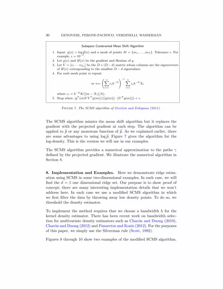
Subspace Constrained Mean Shift Algorithm

1. Input: q(x) = log p(x) and a mesh of points M = {m1, . . . ,mN}. Tolerance ε. Forexample, ε = 10−7.

2. Let g(x) and H(x) be the gradient and Hessian of q.

3. Let V = [v1 · · · vDd ] be the D× (D− d) matrix whose columns are the eigenvectorsof H(x) corresponding to the smallest D − d eigenvalues.

4. For each mesh point m repeat:

m⇐=

(n∑i=1

cih−D

)−1 n∑i=1

cih−DXi

where ci = h−DK(||m−Xi||/h).

5. Stop when: |gT (m)V V T g(m)|/(||g(m)|| · ||V T g(m)||) < ε.

Figure 7. The SCMS algorithm of Ozertem and Erdogmus (2011).

The SCMS algorithm mimics the mean shift algorithm but it replaces thegradient with the projected gradient at each step. The algorithm can beapplied to p or any monotone function of p. As we explained earlier, thereare some advantages to using log p. Figure 7 gives the algorithm for thelog-density. This is the version we will use in our examples.

The SCMS algorithm provides a numerical approximation to the paths γdefined by the projected gradient. We illustrate the numerical algorithm inSection 8.

8. Implementation and Examples. Here we demonstrate ridge estim-ation using SCMS in some two-dimensional examples. In each case, we willfind the d = 1 one dimensional ridge set. Our purpose is to show proof ofconcept; there are many interesting implementation details that we won’taddress here. In each case we use a modified SCMS algorithm in whichwe first filter the data by throwing away low density points. To do so, wethreshold the density estimator.

To implement the method requires that we choose a bandwidth h for thekernel density estimator. There has been recent work on bandwidth selec-tion for multivariate density estimators such as Chacon and Duong (2010),Chacon and Duong (2012) and Panaretos and Konis (2012). For the purposesof this paper, we simply use the Silverman rule (Scott, 1992).

Figures 8 through 10 show two examples of the modified SCMS algorithm.

RIDGE ESTIMATION 31

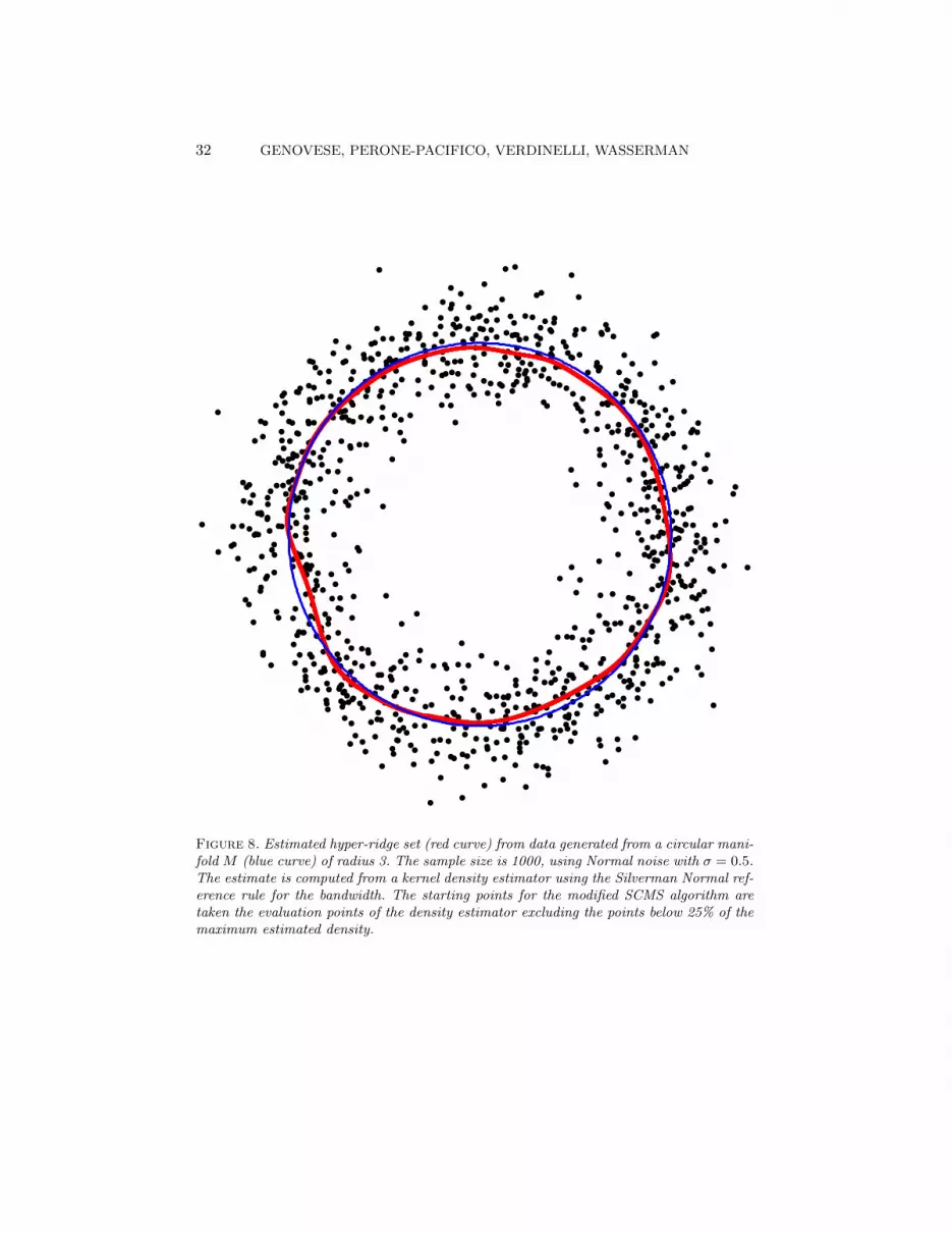
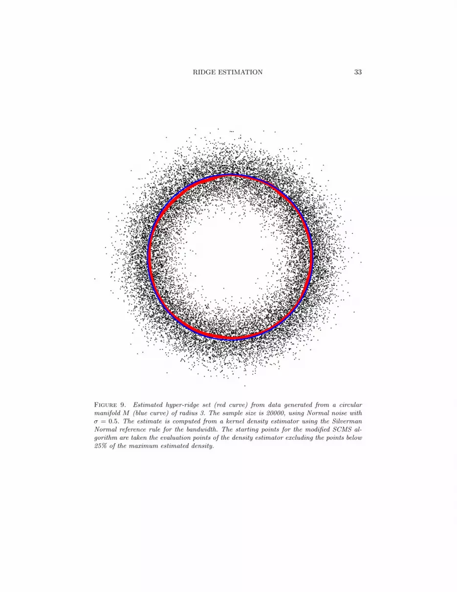
In the first example, the manifold is a circle. Although the circle examplemay seem easy, we remind the reader that no existing statistical algorithmsthat we are aware of can, without prior assumptions, take a point cloud asinput and find a circle, automatically.

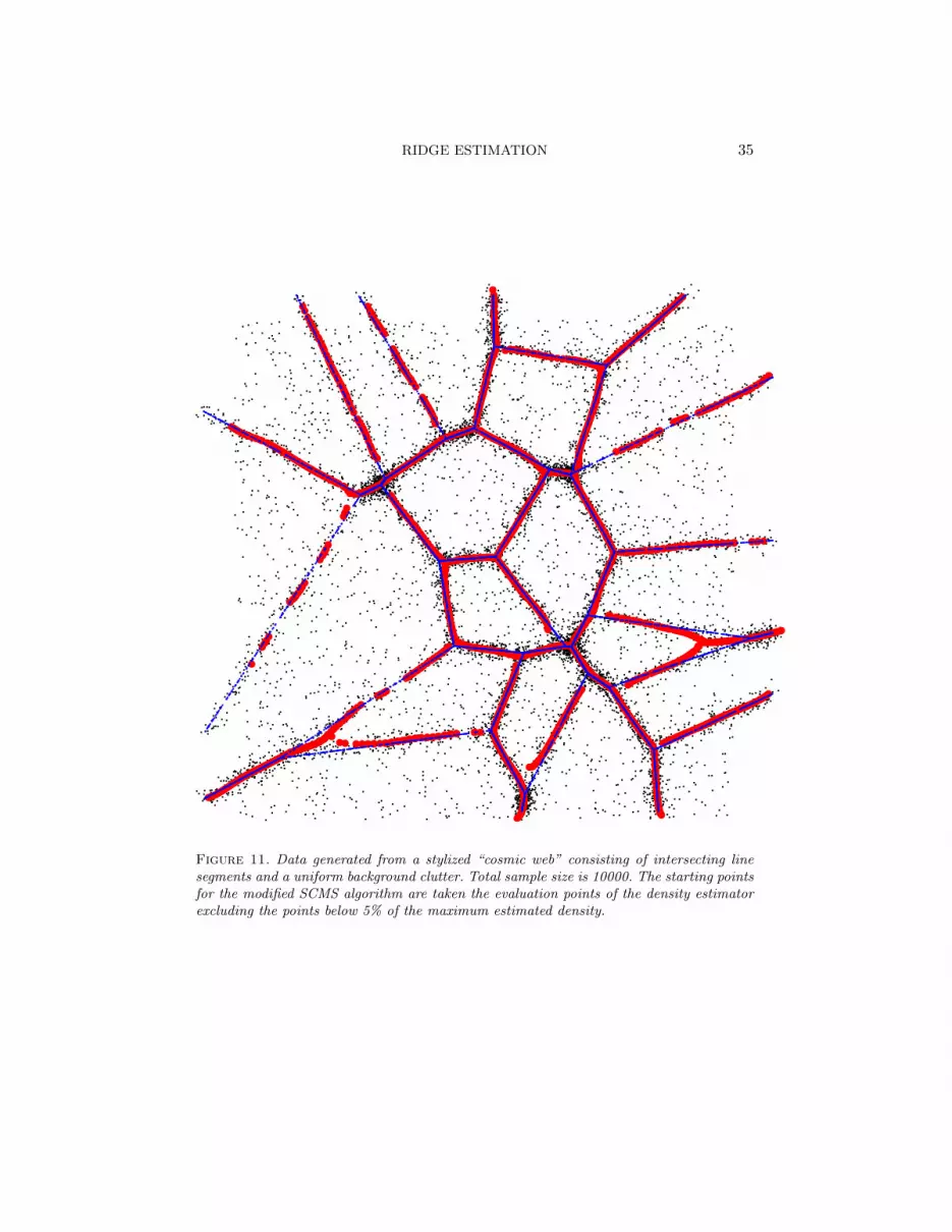
The second example is a stylized “cosmic web” of intersecting line segmentsand with random background clutter. This is a difficult case that violates theassumptions; specifically the underlying object does not have positive reach.The starting points for the SCMS algorithm are a subset of the grid pointsat which a kernel density estimator is evaluated. We select those points forwhich the estimated density is above a threshold relative to the maximumvalue.

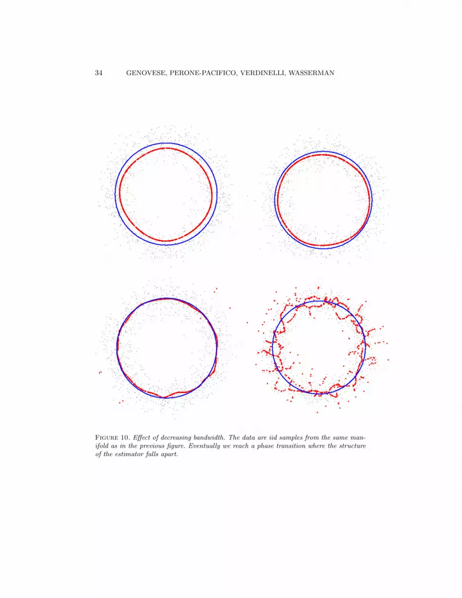
Figure 10 shows the estimator for four bandwidths. This shows an interestingphenomenon. When the bandwidth h is the large, the estimator is biased (asexpected) but it is still homotopy equivalent to the true M . However, when hgets too small, we see a phase transition where the estimator falls apart anddegenerates into small pieces. This suggests it is safer to oversmooth andhave a small amount of bias. The dangers of undersmoothing are greaterthan the dangers of oversmoothing.

The theory in Section 6 required the underlying structure to have positivereach which rules out intersections and corners. To see how the method fareswhen these assumptions are violated, see Figure 11. While the estimator isfar from perfect, given the complexity of the example, the procedure doessurprisingly well.

9. Conclusion. We presented an analysis of nonparametric ridge estima-tion. Our analysis had two main components: conditions that guarantee thatthe estimated ridge converges to the true ridge, and conditions to relate theridge to an underlying hidden manifold.

We are currently investigating several questions. First, we are finding theminimax rate for this problem to establish whether or not our proposedmethod is optimal. Also, Klemela (2005) has derived mode estimation pro-cedures that adapt to the local regularity of the mode. It would be interestingto derive simialr adaptive theory for ridges. Second, the hidden manifold caserequired that the manifold has positive reach. We are working on relaxingthis condition to allow for corners and intersections (often known as strat-ified spaces). Third, we are developing an extension where ridges of eachdimension d = 0, 1, . . . are found sequentially and removed one at a time.


●

●

●

●

●

●●●

●

●

●

●

●

●

●

●

●

●

●

●

●

●

●

●

●

●

●

●

●

●

●

●

●

●

●

●

●

●

●

●

●

●

●

●

●

●

●

●

●

●

●

●

●

●

●

●

●

●

●

●

●

●

●

●

●

●

● ●

●

●

●

●

●

●

●

●

●

●

●

●

●

●

●

●

●

●

●

●

●

●

●

●

●

●

●

●

●

●

●

●

●

●

●

●

●

●

●

●

●

●

●

●

●

●

●

●

●

●

●

●

●

●

●

●

●

●

●

●

●

●

● ●

●

●

● ●

●

●

●

●

●

●

●

●

●

●

●

●

●

●

●

●

●

●

●

●

●

●

●

●

●

●

●

●

●

●

●

●

●

●

●

●

●

●

●

●

●

●

●

●

●

●

●

●

●

●

●

●

●

●

●

●

●

●

●

●

●

●

●

●

●

●

●

●

●

●

●●

●

●

●

●

●

●

●●

●

●

●

●

●

●

●

●●

●

●

●

●

●

●

●

●

●

●

●

●

●

●

●

●

●

●

●

●

●

●

●

●

●

●

●

●

●

●

●

●

●

●

●

●

●

●

●

●

●

●

●

●

●

●

●

●

●

●

●

●

●

●

● ●

●

●

●

●

●

●

●

●

●

●

●

●

●

●

●

●

●

●

●

●

●

●

●

●

●

●

●

●●

●

●

●

●

●

●

●

●

●

●

●

●

●

●

●

●

●

●

●

●

●

●

●

●

●

●

●

●

●

●

●

●

●

●

●

●

●

●

●

●

●

●

●

●

●

●

●

●

●

●

●

●

●

●

●

●

●

●●

●

●

●

●

●

●

●

●

●

●

●

●

●

●

●

●

●

●

●

●●

●●

●

●

●

●

●

●

●

●

●

●

●

●

●

●

●

●

●

●

●

●

●

●

●

●

●

●

●

●

●

●

●

●

●

●

●●

●

●

●

●

●

●

●

●

●●

●

●

●

●

●

●

●

●

●

●

●

●

●

●

●

●

●

●

●

●

●

●

●

●

●

●

●●

●

●

●

●

●

●

●

●

●

●

●

●

●

●●

●

●

●

●

●

●

●

●

●

●

●

●

●

●

●

●

●

●

●

●

●●

●

●

●

●

●

●

●

●

●

●

●

●

●

●

●

●

●

●

●

●

●●

●

●

●

●

●

●

●

●

●●

●

●

●●

●

●

●

●

●

●

●

●

●

●

●

●

●

●

●

●

●

●

●

●

●

●

●

●

●

●

●

●

●

●

●

●

●

●●

●

●

●

●

●

●

●

●

●

●

●

●

●

●

●

●

●

●

●

●

●

●

●

●

●

●

●

●

●

●

●●

●

●

● ●

●

●

●

●

●

●

●

●

●

●

●

●

●

●

●

●

●

●

●

●

●

●

●

●

●

●

●

●

●

●

●

●

●

●

●

●

●

●

●

●

●

●

●

●

●

●

●

●

●

●

●

●

●

●

●

●

●

●

●

●

●

●

●

●

●

●

●

●

●

●

●

●●

●

●

●

●

●

●

●

●

●

●

●

●

●

●

●

●

●

●

●

●

●●

●

●

●

●

●

●

●

●

●

●

●

●

●

●

●

●

●

●

●

●

●

●

●

●

●

●

●

●

●

●

●

●

●

●

●

●

●

●

●

●

●

●

●

●

●

●

●

●

●

●

●

●

●

●

●

●

●

●

●

●

●

●

●

●

●

●

●

●

●

●

●

●

●

●

●

●

●

●

●

●

●

●

●

●

●

●

●

●

●

●

●

●

●

●

●

●

●

●

●

●

●

●

●

●

●

●

●

●

●

●

●

●

●

●

●

●

●

●

●

●●

●

●

●

●

●

●

●

● ●

●

●

●

●

●

●

●

●

●

●

●

●

●

●

●

●

●

●

●

●

●

●

●

●

●

●

●

●

●

●

●

●

●

●

●

●

●

●

●

●

●

●

●

●

●

●

●

●

●

●

●

●

●

●

●

●

●

●

●

●

●

●

●

●

●

●

●

●

●

●

●

●

●

●●

●

●

●

●

●

●

●

●

●

●

●

●

●

●

●

●

●

●

●

●●

●

●

●

●

●

●

●

●

●

●

●

●

●

●

●

●

●

●

●

●

●

●

●

●

●

●

●

●

●

●

●

●

●

●

●

●

●

●

●

●

●

●

● ●

●

●

●

●

●●

●

●

●

●

●

●

●

●

●

●

●

●

●

●

●

●

●

●

●

Figure 8. Estimated hyper-ridge set (red curve) from data generated from a circular mani-fold M (blue curve) of radius 3. The sample size is 1000, using Normal noise with σ = 0.5.The estimate is computed from a kernel density estimator using the Silverman Normal ref-erence rule for the bandwidth. The starting points for the modified SCMS algorithm aretaken the evaluation points of the density estimator excluding the points below 25% of themaximum estimated density.

RIDGE ESTIMATION 33

Figure 9. Estimated hyper-ridge set (red curve) from data generated from a circularmanifold M (blue curve) of radius 3. The sample size is 20000, using Normal noise withσ = 0.5. The estimate is computed from a kernel density estimator using the SilvermanNormal reference rule for the bandwidth. The starting points for the modified SCMS al-gorithm are taken the evaluation points of the density estimator excluding the points below25% of the maximum estimated density.


Figure 10. Effect of decreasing bandwidth. The data are iid samples from the same man-ifold as in the previous figure. Eventually we reach a phase transition where the structureof the estimator falls apart.

RIDGE ESTIMATION 35

●●●●●●●●●

●●●●●●●●●

●●

●●

●●●●●

●●●●

●●●●●

●●●

●●●●●

●

●●●

●●●●●

●●

●●●●●●

●●

●●

●●●●●

●●

●●

●●●●●

●●●

●●●●●

●●●

●●●●●

●●●

●●●●●

●●●

●●●

●●●●●

●●●

●●●

●●●●●

●●●

●●

●●

●●●●

●●●

●●●

●●●●●

●●●●

●●

●●

●●●●●●

●●●

●●●

●●●

●●●●●

●

●●●

●●●

●●●●●●●

●●●●

●

●●●

●●

●●●

●

●

●●●

●●

●●

●●

●

●●●

●●

●●●

●●●●

●●

●●●

●●

●●●●

●●●●●●

●

●●●

●●●●●●

●●

●●

●

●●●●●●

●●

●●

●●

●●●●●●●

●

●●●●●●●

●●●

●●●

●●●●●●●

●●

●●●

●●●

●

●

●●●

●●●●●●●

●●

●

●●●

●●

●●

●●

●●●●●●

●

●●

●●●

●●●●

●●●●

●●

●●

●●●

●●●

●●●●

●●

●●●

●●●●

●●

●●

●●

●●●

●

●●●●

●

●●●●

●●●

●●

●●

●●

●●●

●●●

●●●●

●

●●●●●

●●●

●●

●●●

●●●

●●●●

●●●

●●●●●

●

●●●

●●●

●●●

●●●●

●●●

●●●●●

●

●●

●●●

●

●●●

●●●●

●●●●●

●

●●

●●

●●●

●●●

●●●●

●●●

●●●

●●●●

●●

●●●●

●

●●

●●●●

●●●●●●●●●●●

●●●●

●●●●●●

●●

●●

●●●

●●●●●●●●●●●●●●●●●●

●

●●●●●●●

●●●

●●●●●●●●●●●●●●●●●●●●●

●●●●●●●

●●

●●●●●●●●●●●●●

●●●●●●

●●●●●●

●●●●●●

●●●●●

●●●●●●●

●●●●●

●●●●●●

●●●●●●●●●

●●●

●●●●●

●●●●●

●●●●●●●●●●●●

●● ●●

●●●●●

●●●●●●

●●●●

●●●●●●●●●●●●

●●

●●●●●●●●

●●●●●●

●●●●●●

●●●●●

●●●●●●●●●●●●●●●●●●●●●●●●

●●●●●●●●●●●

●●●●●

●●●●●●

●●●●●

●●●●●●●●●●●●●●●●●●●●●

●●●

●●●●●●●●●●●●●

●●●●●

●●●●

●●●

●

●●●●●

●

●●●●●●●●●●●●●●

●●

●●

●●

●●●●●●●●●●●●●●

●●●●●

●●●●

●

●●●

●●●●

●●●●●

●●●●●●●●●●●●●

●●●●●

●●

●●●

●●

●●●●●●●●●●

●●●●●

●●●●

●●●

●●●●●●●●

●●●●●

●●●●

●●●●●●●

●●●

●●

●●●●●●●

●●●●●

●●●●

●●●

●●●●●●●●

●●●●●

●●●

●●●●●●●●

●●●

●●●●●●●●●●

●●●●

●●

●●●●●●●●●

●●●●●

●●●

●●●●●●●●

●●

●

●

●●●●●●

●●●●

●

●●●●●●●●●

●●●●●

●●

●●●●●●●

●●

●

●●●●●●

●●

●●●●

●●●●●

●●●

●●●●●

●●●

●●●●●

●●

●●●●●

●●

●●●●●●

●●

●●●

●●

●●●

●●●

●●●●

●●●

●●●●●●

●●●●●●

●●●●

●●

●●●●●●●●

●●●

●●●●●●●●

●●●●●●

●●●

●

●●●●●●●

●●

●●●●●●●●

●●●●●●●●

●

●●●●●●●

●

●●●●●●●●

●●●●●●●●

●●●●●●●

●

●●●●●●●●

●●

●●●●●●●

●

●●

●●●●●●

●●●

●●●●

●●●●●●●

●●●

●●●●

●●●●

●●●

●●●●●●●●●●●●●

●●●●

●●●●

●●●●●

●●

●

●●●●

●●●●

●●

●●

●●●●

●●●●●●●●●●

●●●●

●

●●●●●

●●●

●

●●●●●

●●●●●

●●

●●

●●

●●●

●●●●●●●●●●●●●●●

●●●●

●●●●●

●●

●●

●●●●●

●●●●●●●●

●●

●●

●●

●●

●●●

●●●●●●●●●●●●

●●●●

●●●●●

●●

●●●●●●●●●●●●●●

●●

●●

●●

●●

●

●●

●●●●●●●●●●

●●●

●●●●●

●●●

●●●●●●●●●●●●●●●

●●

●●

●●

●

●●●●●●●●●●

●

●●

●●●●●

●

●●●●

●●●●●●●●

●●●●

●

●●●

●●●●

●●●

●●●

●●●

●●●

●●●●●●●●●●

●

●●●●●

●

●●●

●●●●●●●

●●●

●●●●●●●

●●

●●●●

●

●●●●

●●

●●●

●●●

●●●

●●●●

●●

●●●●

●

●●●

●●●

●●

●●●

●●●

●●●●

●●

●●●●

●

●●

●●●●

●●●

●●●

●●●

●●●●

●●

●●●●

●

●●●●●●●●●●●

●●●●

●●

●●

●●

●●●●

●●

●●●●

●

●●●●●●●●●●●●●

●●●●

●●

●●

●●●●

●

●●●●

●●●●●●●●●●●●●●●●

●●●

●●●

●●●●

●●

●●●●

●●●●●●●●●●●●●

●●●

●●●

●●●

●●●

●

●●●●

●

●●●●●●

●●●●●

●●●●

●●●

●●●●

●●●●

●●●●●

●●●●

●●●

●●●●

●●

●●●●

●●●●

●●●

●●●

●●●●

●●

●●●●

●●●

●●●

●●●

●●●

●●

●●

●●●

●●●

●●●

●●●

●●●●●●●●

●●●

●●

●●●●

●●●●●●●

●●●

●●●

●●●●●

●●●●●●

●●●

●●●

●●●●

●●●●●●

●●●

●●

●●●

●●●●●

●●●

●

●●●●

●●●●●

●●●

●●

●●●

●●●●●

●●●

●●●

●●●●

●●●●●

●●

●●●

●●●●●

●●

●●●●

●●●●●

●●

●●

●●●●

●●●●●

●●

●●

●●●●

●●●●●

●

●●

●●

●●●●●

●●

●●●●●●

Figure 11. Data generated from a stylized “cosmic web” consisting of intersecting linesegments and a uniform background clutter. Total sample size is 10000. The starting pointsfor the modified SCMS algorithm are taken the evaluation points of the density estimatorexcluding the points below 5% of the maximum estimated density.


This leads to a decomposition of the point cloud into structures of increas-ing dimension. Finally, there are a number of methods for speeding up themean shift algorithm. We are investigating how to adapt these speedups forSCMS.

Appendix: Proof of Lemma 10. The gradient is

(61) gσ(x) = − 1

σ2

∫M

(x− z)φσ(x− z)dW (z)

and the Hessian is

Hσ(x) = − 1

σ2

∫M

(I − (x− z)(x− z)T

σ2

)φσ(x− z)dW (z)

= − 1

σ2

[pσ(x)I − 1

σ2

∫M

(x− z)(x− z)Tφσ(x− z)dW (z)

].(62)

We can partition Mσ into disjoint fibers. Choose an x ∈ Mσ and let x bethe unique projection of x onto M . Let B = B(x,Kσ). For any boundedfunction f(x, z),

(63)

∫M∩Bc

f(x, z)φσ(x− z)dW (z) ≤ C

(2π)D2

e−K2σ/(2σ

2)

σDW (Bc) ≤ CσA.

Let T = TxM denote the d-dimensional tangent space at x and let T⊥

denote the (D − d)-dimensional normal space. For z ∈ B ∩M , let z be theprojection of z onto T . Then

(64) x− z = (x− x) + (x− z) + (z − z) = dM (x)u+ (x− z) +R

where u = (x − x)/dM (x) ∈ T⊥ and R = (z − z). (Recall that dM is thedistance function; see (7).) For small enough σ, the map h taking z to zis a bijection B ∩M and so the distribution W induces a distribution W ,that is, W (A) = W (h−1(A)). Let w denote the density of W with respectto Lebesgue measure µd on T . The density is bounded above and below andhas two continuous derivatives.

Lemma 12. For every x ∈ R⊕ σ, supz∈B ||z − z|| ≤ cK2σ.

Proof. Choose any z ∈ B and let z be its projection onto T . Because thereach is κ > 0, there exists a ball S(a, κ) ⊂ RD such that a is in the plane

RIDGE ESTIMATION 37

defined x, z and z, S(a, κ) is tangent to the manifold at x and S(a, κ) doesnot intersect M except at x. Consider the line through z and z and let zabe the point where the line intersects S(a, κ). Now ||za − z|| ≥ ||z − z|| andby elementary geometry, ||za − z|| ≤ CK2

σ.

Recall that rσ = ασ with 0 < α < 1. Define the following quantities:

β =e−α

2/2(1− α2)

2σD−d+2, σ = σ log3

(1

σD+A

)φ⊥(u) =

e−||u||2/(2σ2)

(2π)D−d

2 σD−d, φ‖(w) =

e−||w||2/(2σ2)

(2π)d2σd

pσ,B(x) =

∫M∩B

φσ(x− z)dW (z) B = B(x,Kσ)

where u ∈ RD−d and w ∈ Rd.

Lemma 13. We have that

(65) φσ(x− z) = φ⊥(x− x)φ‖(x− z)(1 +O(σ)).

Proof. First note that, for all x ∈ Rσ,

(66)1

(2π)D−d

2

e−α2/2

σD−d≤ φ⊥(x− x) ≤ 1

(2π)D−d

2

1

σD−d

and so, φ⊥(x− x) � σ−(D−d) as σ → 0. Now,

||x− z||2 = ||x− x||2 + ||x− z||2 + ||z − z||2 + 2〈x− x, z − z〉,

we have that

φσ(x− z) = φ⊥(x− x)φ‖(x− z)e−||z−z||2/(2σ2)e−〈x−x,z−z〉/σ

2.

Now ||z − z||2 = O(K4σ) and |〈x − x, z − z〉| ≤ ||x − x|| ||z − z|| = O(σK2

σ)and so

e−||z−z||2/(2σ2)e−〈x−x,z−z〉/σ

2= (1 +O(σ)).


Proof of the Lemma 10.1. From (63), pσ(x) =

∫M∩B φσ(x− z)dW (z) +O(σA). Now∫

M∩Bφσ(x− z)dW (z) = (1 +O(σ))φ⊥(x− x)

∫M∩B

φ‖(x− z)dW (z)

= (1 +O(σ))φ⊥(x− x)

∫TM∩B

φ‖(x− z)w(z)dµd(z)

= (1 +O(σ))φ⊥(x− x)

∫A

1

(2π)d/2e−||t||

2/2w(x+ σt)dµd(t)

where A = {t = (z − x)/σ : z ∈ B}. The volume of A is O(σD+A) andA→ Rd as σ → 0. Also, w(x+ σt) = w(x) +O(σ). Hence,∫

Aw(x+ σt)dµd(t) = (w(x) +O(σ))(1−O(σD+A))

and so∫M∩B

φσ(x− z)dW (z) = φ⊥(x− x)(1 +O(σ))(w(x) +O(σ))(1−O(σD+A))

and

pσ(x) = φ⊥(x− x)(1 +O(σ))(w(x) +O(σ))(1−O(σD+A)) +O(σA)

= φ⊥(x− x)(1 +O(σ)).

2. pσ,B(x). This follows since in part 1 we showed that pσ,B(x) = pσ(x) +O(σA).

3. For the gradient we have

−σ2gσ(x) =

∫(x− z)φσ(x− z)dW (z)

= (x− x)

∫φσ(x− z)dW (z) +

∫(x− z)φσ(x− z)dW (z) +

∫(z − z)φσ(x− z)dW (z)

= I + II + III.

Now, I = (x− x)pσ(x) = (x− x)φ⊥(x− x)(1 +O(σ)) and

II =

∫M∩B

(x− z)φσ(x− z)dW (z) +O(σA)

= (1 +O(σ))φ⊥(x− x)

∫M∩B

(x− z)φ‖(x− z)dW (z) +O(σA).

RIDGE ESTIMATION 39

For some u between x and z we have∫M∩B

(x− z)φ‖(x− z)dW (z) = σ

∫M∩B

x− zσ

φ‖(x− z)dW (z)

= σ

∫h−1(B)

x− zσ

φ‖(x− z)w(z)dµd(z)

= σ

∫At

1

(2π)d/2e−||t||

2/2w(x+ σt)dµd(t)

= σ

∫At

1

(2π)d/2e−||t||

2/2[w(x) + w′(x)σt+ w′′(u)σ2t2/2]dµd(t)

= O(σ2)

where A = {t = (z − x)/σ ∈ h−1(B)}. Finally,

III =

∫M∩B

(z−z)φσ(x−z)dW (z)+O(σA) = φ⊥(x−x)O(K2σ)+O(σA) = O(K2

σ)φ⊥(x−x).

Hence,

−σ2gσ(x) = (x−x)pσ(x)+O(σ2)+φ⊥(x−x)O(K2σ) = pσ(x)((x−x)+O(K2

σ))

and hence

gσ(x) = − 1

σ2pσ(x)

((x− x) +O(K2

σ)).

It follow from part 1 that ||gσ(x)|| = O(σ−(D−d−1)).

4. To find the eigenvalues, we first approximate the Hessian. Without loss ofgenerality, we can rotate the coordinates so that T is spanned by e1, . . . , ed,T⊥ is spanned by ed+1, . . . , eD and u = (0, . . . , 0, 1). Now,

−σ2Hσ(x)

pσ(x)= I −

∫(x− z)(x− z)Tφσ(x− z)dW (z)

σ2∫φσ(x− z)dW (z)

and ∫M∩Bc

(x− z)(x− z)Tφσ(x− z)dW (z) = O(σA).

Let Q =∫M∩B(x − z)(x − z)Tφσ(x − z)dW (z). Then, from (64), we have

Q = Q1 +Q2 +Q3 +Q4 +Q5 +Q6 where

Q1 = d2M (x)uuT

∫M∩B

φσ(x− z)dW (z) Q2 =

∫M∩B


Q3 =

∫M∩B

(z − z)(z − z)Tφσ(x− z)dW (z) Q4 =

∫M∩B

(x− x)(x− z)Tφσ(x− z)dW (z)

Q5 =

∫M∩B

(x− x)(z − z)Tφσ(x− z)dW (z) Q6 =

∫M∩B

(x− z)(z − z)Tφσ(x− z)dW (z).


First, we note that

Q1 = d2M (x)uuTφ⊥(x− x)(1 +O(σ)).

Next,

Q2 =

∫M∩B


= (1 +O(σ))φ⊥(x− x)

∫M∩B

(x− z)(x− z)Tφ‖(x− z)dW (z)

and∫M∩B

(x− z)(x− z)Tφ‖(x− z)dW (z) =

∫h−1(B)

(x− z)(x− z)Tφ‖(x− z)w(z)dµd(z)

= w(x)

∫h−1(B)

(x− z)(x− z)Tφ‖(x− z)dµd(z) +O(K5σ).

Next, with t = (t1, . . . , td, 0, . . . , 0),∫h−1(B)

(x− z)(x− z)Tφ‖(x− z)dµd(z) = σ2

∫BttT (2π)−d/2e−||t||

2/2dµd(t)

= σ2

(∫ttT (2π)−d/2e−||t||

2/2dµd(t)−∫BcttT (2π)−d/2e−||t||

2/2dµd(t)

)

= σ2

([Id 00 0

]+O(σA+D)

)

and so

Q2 = (1 +O(σ))φ⊥(x− x)σ2

([Id 00 0

]+O(σA+D)

).

A similar analysis on the remaining terms yields:

Q3 = (1 +O(σ))φ⊥(x− x)O(K4σ)

Q4 = (1 +O(σ))φ⊥(x− x)O(σK2σ)

Q5 = (1 +O(σ))φ⊥(x− x)O(σK2σ)

Q6 = (1 +O(σ))φ⊥(x− x)O(K3σ).

RIDGE ESTIMATION 41

Combining all the terms we have

Q = (1 +O(σ))φ⊥(x− x)

(d2M (x)uuT + σ2

([Id 00 0

]+O(σA+D)

))+O

(σK2

σ

).

Hence,

Hσ(x) = −(1+O(σ))pσ(x)

σ2

0 · · · 0 0 · · · · · · · · · 0...

. . .... 0 · · · · · · · · · 0

0 · · · 0 0 · · · · · · · · · 0

0 · · · 0 1 0 · · · · · · 00 · · · 0 0 1 · · · · · · 0

0 · · · 0 0 0. . . · · · 0

0 · · · 0 0 0 · · · 1 0

0 · · · 0 0 0 · · · 0 1− d2M (x)

σ2

+O (σ)

.

The result follows.

5. This follows from part 4 and the Davis-Kahan theorem.

6. From part 5, Lσ(x) = L† + E where L† =

[0d×d 0d,D−d

0D−d,d ID−d

]and E =

O (σ). Hence, Gσ(x) = Lσ(x)gσ(x) = (L† + E)gσ(x) and the result followsfrom parts 3 and 4.

7. These follow from part 4.

8. Now we turn to ||H ′σ||. Let ∆ = (x− z). We claim that

H ′ =1

σ4

∫ [(Φ⊗ I)(I ⊗∆ + ∆⊗ I)− φσ(∆)

σ2(I ⊗∆∆T )(vec(I)⊗∆T )

]dW (z)

+1

σ4

∫φσ(∆)(vec(I)⊗∆T )dW (z).

To see this, note first that H = 1σ4Q− 1

σ2A where

(67) Q =

∫(x− z)(x− z)Tφσ(x− z)dW (z) and A = pσ(x)I.

Note that Q =∫

(x− z)(x− z)TΦdW (z) where Φ = φσ(∆)ID. So

Q′ =

∫(d/dx)[(x− z)(x− z)TΦ]dW (z)


andd

dx[(x− z)(x− z)TΦ] =

d(x− z)(x− z)TΦ

dx=d∆∆TΦ

d∆.

Now (d/dx)(∆∆TΦ) = (fg)′ where f = ∆∆T and g = Φ and so

d

dx(∆∆TΦ) = (Φ⊗ I)

d

dx(∆∆T ) + (I ⊗∆∆T )

d

dxΦ

= (Φ⊗ I)(I ⊗∆ + ∆⊗ I)− φσ(∆)

σ2(I ⊗∆∆T )(vec(I)⊗∆T ).

Hence

Q′ =

∫ [(Φ⊗ I)(I ⊗∆ + ∆⊗ I)− φσ(∆)

σ2(I ⊗∆∆T )(vec(I)⊗∆T )

]dW (z).

By a similar calculation,

A′ = − 1

σ2


Thus,

H ′ =1

σ4Q′ − 1

σ2A′

=1

σ4

∫ [(Φ⊗ I)(I ⊗∆ + ∆⊗ I)− φσ(∆)

σ2(I ⊗∆∆T )(vec(I)⊗∆T )

]dW (z)

+1

σ4


Each of these terms is of order O(supx∈M ||w′′(x)||/σD−d+1). Consider thefirst term

1

σ4

∫(Φ⊗ I)(I ⊗∆)dW (z) =

1

σ4+D(2π)D/2

∫e−||x−z||

2/(2σ2)(I ⊗∆)dW (z)

=1

σ3+D(2π)D/2

∫e−||u||

2/2(I ⊗ u)dW (z)

where u = (x − z)/σ. As in the proof of part 1, we can restrict to B ∩M ,do a change of measure to W and the term is dominated by

1

σ3+D−d(2π)D/2

∫Ae−||u||

2/2(I ⊗ u)

[w(x) + w′(u)σu

]dµd(t)

=C

σ3+D−d(2π)D/2.

The other terms may be bounded similarly.

RIDGE ESTIMATION 43

References.

Adams, H., Atanasov, A. and Carlsson, G. (2011). Morse theory in topological dataanalysis. arXiv preprint arXiv:1112.1993.

Bendich, P., Wang, B. and Mukherjee, S. (2012). Local homology transfer and strat-ification learning. In Proceedings of the Twenty-Third Annual ACM-SIAM Symposiumon Discrete Algorithms. SIAM, 1355–1370.

Bhatia, R. (1997). Matrix analysis, vol. 169. Springer Verlag.Cadre, B. (2006). Kernel estimation of density level sets. Journal of multivariate analysis,

97 999–1023.Caillerie, C., Chazal, F., Dedecker, J. and Michel, B. (2011). Deconvolution for

the Wasserstein metric and geometric inference. INRIA Technical report 7678.Carreira-Perpinan, M. and Williams, C. (2003). On the number of modes of a gaus-

sian mixture. In Scale Space Methods in Computer Vision. Springer, 625–640.Chacon (2012). Clusters and water flows: a novel approach to modal clustering through

morse theory. arXiv preprint arXiv:1212.1384.Chacon, J. and Duong, T. (2010). Multivariate plug-in bandwidth selection with un-

constrained pilot bandwidth matrices. Test, 19 375–398.Chacon, J. and Duong, T. (2012). Bandwidth selection for multivariate density de-

rivative estimation, with applications to clustering and bump hunting. arXiv preprintarXiv:1204.6160.

Chacon, J., Duong, T. and Wand, M. (2011). Asymptotics for general multivariatekernel density derivative estimators. Statistica Sinica, 21 807–840.

Chazal, F., Cohen-Steiner, D. and Lieutier, A. (2009). A sampling theory for com-pact sets in euclidean space. Discrete & Computational Geometry, 41 461–479.

Chazal, F., Guibas, L., Oudot, S. and Skraba, P. (2011). Persistence-based cluster-ing in riemannian manifolds. In Proceedings of the 27th annual ACM symposium onComputational geometry. ACM, 97–106.

Chazal, F. and Lieutier, A. (2005). The λ-medial axis. Graphical Models, 67 304–331.Chen, X., Qi, H. and Tseng, P. (2003). Analysis of nonsmooth symmetric-matrix-valued

functions with applications to semidefinite complementarity problems. SIAM Journalon Optimization, 13 960–985.

Cheng, M., Hall, P. and Hartigan, J. (2004). Estimating gradient trees. LectureNotes-Monograph Series 237–249.

Comaniciu, D. and Meer, P. (2002). Mean shift: a robust approach toward feature spaceanalysis. Pattern Analysis and Machine Intelligence, IEEE Transactions on, 24 603–619.

Davenport, M., Hegde, C., Duarte, M. and Baraniuk, R. (2010). Joint manifoldsfor data fusion. Image Processing, IEEE Transactions on, 19 2580–2594.

Dumbgen, L. and Walther, G. (2008). Multiscale inference about a density. The Annalsof Statistics, 36 1758–1785.

Edelsbrunner, H., Fasy, B. T. and Rote, G. (2012). Add isotropic gaussian kernelsat own risk: More and more resiliant modes in higher dimensions. In ACM Symposiumon Computational Geometry (SoCG 2012). To Appear.

Fukunaga, K. and Hostetler, L. D. (1975). The estimation of the gradient of a densityfunction, with applications in pattern recognition. IEEE Transactions on InformationTheory, 21 32–40.

Genovese, C., Perone-Pacifico, M., Verdinelli, I. and Wasserman, L. (2009). Onthe path density of a gradient field. The Annals of Statistics, 37 3236–3271.


Genovese, C., Perone-Pacifico, M., Verdinelli, I. and Wasserman, L. (2012a). Thegeometry of nonparametric filament estimation. Journal of the American StatisticalAssociation, 107 788–799.

Genovese, C. R., Perone-Pacifico, M., Verdinelli, I. and Wasserman, L. (2012b).Manifold estimation and singular deconvolution under hausdorff loss. The Annals ofStatistics, 40 941–963.

Genovese, C. R., Perone-Pacifico, M., Verdinelli, I. and Wasserman, L. (2012c).Minimax manifold estimation. Journal of Machine Learning Research 1263–1291.

Gine, E. and Guillou, A. (2002). Rates of strong uniform consistency for multivariatekernel density estimators. In Annales de l’Institut Henri Poincare (B) Probability andStatistics, vol. 38. Elsevier, 907–921.

Hall, P., Peng, L. and Rau, C. (2001). Local likelihood tracking of fault lines andboundaries. Journal of the Royal Statistical Society: Series B (Statistical Methodology),63 569–582.

Hall, P., Qian, W. and Titterington, D. (1992). Ridge finding from noisy data.Journal of Computational and Graphical Statistics 197–211.

Horn, R. A. and Johnson, C. R. (2013). Matrix Analysis: Second Edition. Cambridge.Irwin, M. (1980). Smooth dynamical systems, vol. 94. Academic Press.Klemela, J. (2005). Adaptive estimation of the mode of a multivariate density. Journal

of Nonparametric Statistics, 17 83–105.Klemela, J. (2009). Smoothing of multivariate data: density estimation and visualization,

vol. 737. Wiley.Li, J., Ray, S. and Lindsay, B. (2007). A nonparametric statistical approach to clustering

via mode identification. Journal of Machine Learning Research, 8 1687–1723.Magnus, X. and Neudecker, H. (1988). Matrix differential calculus. New York.Niyogi, P., Smale, S. and Weinberger, S. (2006). Finding the homology of sub-

manifolds with high confidence from random samples. Discrete and ComputationalGeometry, 39 419–441.

Ozertem and Erdogmus (2011). Locally defined principal curves and surfaces. Journalof Machine Learning Research, 12 1249–1286.

Panaretos, V. and Konis, K. (2012). Nonparametric construction of multivariate ker-nels. Journal of the American Statistical Association, 107 1085–1095.

Polonik, W. (1995). Measuring mass concentrations and estimating density contourclusters-an excess mass approach. The Annals of Statistics 855–881.

Prakasa Rao, B. (1983). Nonparametric functional estimation. Academic Press, NewYork.

Scott, D. (1992). Multivariate density estimation. Multivariate Density Estimation,Wiley, New York, 1992, 1.

Stewart, G. and Sun, J. (1990). Matrix perturbation theory. Academic press New York.Von Luxburg, U. (2007). A tutorial on spectral clustering. Statistics and computing, 17

395–416.Walther, G. (1997). Granulometric smoothing. The Annals of Statistics 2273–2299.Wegman, E. and Luo, Q. (2002). Smoothings, ridges, and bumps. Proceedings of the

ASA (published on CD). Development of the relationship between geometric aspects ofvisualizing densities and density approximators, and a discussion of rendering and light-ing models, contouring algorithms, stereoscopic display algorithms, and visual designconsiderations.

Yukich, J. (1985). Laws of large numbers for classes of functions. Journal of multivariateanalysis, 17 245–260.

RIDGE ESTIMATION 45

Department of StatisticsCarnegie Mellon UniversityPittsburgh, PA 15213E-mail: [email protected]

Department of Statistical SciencesSapienza University of RomeRome, ItalyE-mail: [email protected]

Department of StatisticsCarnegie Mellon UniversityPittsburgh, PA 15213and Department of Statistical SciencesSapienza University of RomeRome, ItalyE-mail: [email protected]

Department of StatisticsCarnegie Mellon UniversityPittsburgh, PA 15213E-mail: [email protected]

mailto:[email protected]




Documents

Nonparametric ridge estimation