Embed Size (px)
Citation preview
Bounds for Ruin Probabilities and Value at Risk
By
Samuel H. Cox, Yijia Lin, Ruilin Tian and Luis F. Zuluaga
July 29, 2007
Please address correspondence to Ruilin TianDepartment of Risk Management & InsuranceGeorgia State UniversityP.O. Box 4036Atlanta, GA 30302-4036 USAEmail: [email protected]
Samuel H. CoxUniversity of ManitobaEmail: sam [email protected]
Yijia LinUniversity of Nebraska - LincolnEmail: [email protected]
Ruilin TianGeorgia State UniversityEmail: [email protected]
Luis F. ZuluagaUniversity of New BrunswickEmail: [email protected]
ACKNOWLEDGEMENTSThis research work was supported by the Actuarial Foundation, and the CasualtyActuarial Society. The last author was also partially supported by NSERC grant290377.
BOUNDS FOR RUIN PROBABILITIES AND VALUE AT RISK
ABSTRACT. In many situations, complete information about a rare event is not available,meaning the underlying probability distribution is not completely specified. This paperfinds the best one can do when the incomplete information consists of estimates of thefirst two moments of the distribution. These are called semiparametric lower and upperbounds. We consider value-at-risk (VaR) in the sense that we find bounds on probability ofportfolio return less than some small value, given only the first two moments of the portfoliocomponents. We also apply semiparametric bounds to a rare event hitting an insurer forwhich losses are extraordinary high and investment income is low. We refer to this as “ruin”although the company may survive; it is just a convenient way to describe a rare event thatwould threaten a company’s solvency. In addition, we calculate bounds on insurance stop-loss payments. The payoff of a call or put option can be considered as a special case ora transform of the stop-loss payment. In order to numerically solve the semiparametricbounds considered here, we reformulate the corresponding semiparametric bound problemas a sum of squares (SOS) program. A SOS program is an optimization problem wherethe variables are coefficients of polynomials, the objective is a linear combination of thevariable coefficients, and the constraints are given the polynomials being SOS. This form ofreformulation allows us to use one of several readily available SOS programming solvers tosolve the moment problem. For the stop-loss bound problem, Cox (1991)’s method is alsoinvestigated to confirm our SOS program solutions. Our numerical examples have shownthat our technique works reasonably well.
1. INTRODUCTION
Sometimes, rare things happen and the least expected occurs. Indeed, some events occur once ortwice in a lifetime — leaving little room to learn from experiences. In financial markets, extremeevents, no matter how rare, could have a profound impact on a company or even the whole country(Liu, Pan, and Wang, 2005). One such example is the Asian currency crisis of 1997, largelyattributed to over-expansion of corporate credit with un-hedged short-term borrowing from abroad;large amounts of unproductive capital investments; and speculation on overvalued assets and largetrade deficits (Hong, 1998). In 1997, the value of Thai baht fell by 48.49%, Korean won dropped47.46% and Malaysian ringgit fell by 35.36%.
Insurers are also not free from the impact of catastrophic large-scale extreme events. For exam-ple, the total loss of the tragic September 11 terrorist attacks exceeded $80 billion with the insuredlosses amounting $40.2 billion (Yu and Lin, 2007). As for mortality risks, a recent example ofunanticipated catastrophe death losses is the devastating earthquake and tsunami across southernAsia and eastern Africa in December 26, 2004. The 2004 Indonesian population death index in-creased by 16.58% relative to the 2003 level (Cox, Lin, and Wang, 2006). The excess populationmortality death rate is even higher for Sri Lanka, about 34%. Cummins and Doherty (1997) raise
Date: July 29, 2007.1
2 BOUNDS FOR RUIN PROBABILITIES AND VALUE AT RISK
concerns about the financial stability of the insurance industry before these recent catastrophicevent, so the concern is even greater now.
As a result, with pervasive economic and financial revolutions sweeping our world and potentialdevastative catastrophes, the increasing interest in tail risk management is fuelled by practical is-sues, including investment downside risk and insurance catastrophe risk. Managing extreme lossescaused by catastrophic events like U.S. stock market crash in 1929, hurricanes and earthquakeshas been a major concern for market participants. Thus, developing statistical techniques to modelextreme investment and insurance losses is certainly a major task for risk managers.
Unfortunately, our knowledge about the true distribution is limited. As such, increasing efforthas been made to incorporate moment methodology into analysis without distribution assumptions.Among the first applications of the moment problem approach to practical problems were doneby Scarf (1958) (inventory management) and Lo (1987) (mathematical finance). In particular,existing applications of moment theory in finance focus on option pricing to extend the well-known Black and Scholes (1973) formula (Merton, 1973; Perrakis and Ryan, 1984; Levy, 1985;Ritchken, 1985; Lo, 1987; Boyle and Lin, 1997; Bruckner, 2007; Gerber, Shiu, and Smith, 2007;Schepper and Heijnen, 2007) and other asset pricing and portfolio problems (Gallant, Hansen, andTauchen, 1990; Hansen and Jagannathan, 1991; Ferson and Siegel, 2001, 2003). Brockett and Cox(1985); Cox (1991); Brockett, Cox, and Smith (1996) and Roos (2007) apply moment method ininsurance. Bertsimas and Popescu (2005) give a review of the literature and historical perspectiveon this method, which covers developments from Chebyshev and Markov in the late 1800s tobreak-throughs in the last 10 years. However, very few papers use the moment method to studyextreme financial and insurance events. Traditional statistical methods based on the estimation ofthe entire density are inappropriate for such tasks because these methods typically produce a goodfit in those regions in which most of the data reside but at the expense of good fit in the tails (Hsieh,2004). Therefore, the purpose of our paper is to apply moment methods to estimate the joint eventssuch as concurrent extreme investment loss and insurance loss.
A novel aspect of this article is that it takes into account the correlation between different assetsand insurance lines of business. Usually, models on risk-based capital and enterprise risk man-agement decisions involve several random variables, such as losses, stock prices, interest rates,currency exchange rates and so on. There is an active interest in obtaining information on ex-tremes of joint distributions of these random variables. For example, the insurer would like toknow the probability of having a large loss payments exceeding a given threshold and a loss intheir asset investment below a certain level at the same time. Therefore, the aim of the presentpaper is to explicitly solve the upper and lower bounds on the probability of such a joint event,given the first two sets of moments of the joint distribution. In other words it involves not only thevariances of the individual asset returns and/or insurance margins but also their covariances.
BOUNDS FOR RUIN PROBABILITIES AND VALUE AT RISK 3
In particular, suppose that X1 and X2 denote random variables in a model such as a randominvestment return and a random future insurance benefit payment. The variables may be depen-dent. For example, if the loss payment is subject to economic inflation, then it is correlated withinvestment return and the discount factor. In another example, the variables X1 and X2 may besecurity returns such as S&P 500 and Nikkei Index returns respectively. A risk manager might beinterested in measuring the joint distribution of extreme values of X1 and X2. That is, X1 and X2
simultaneously take very high values. A third example comes from a stop-loss payment φ(X1, X2)
with the form
(1) φ(X1, X2) =
b if X1 +X2 ≥ a+ b
X1 +X2 − a if a ≤ X1 +X2 ≤ a+ b
0 if X1 +X2 ≤ a.
Since the maximum claim amounts b will be paid when X1 +X2 ≥ a+ b, the reinsurer may wantto know something about his expected payments. One way to estimate these measures is to use theobservations of X1 and X2 to derive parameters of an assumed distribution (typically joint normal)and then reach an extreme measure of the joint distribution. In many instances, however, the lowfrequency of observations for X1 and X2 means that it is impossible to reach sound conclusionswith the parametric approach. Even if a plenty of observations of X1 and X2 are available, for ex-ample, given day-to-day price observations, assuming a particular distribution for joint distributionof X1 and X2 might be perilous, specially when we are interested in estimating extreme joint dis-tributions such as tail probabilities and value at risk (VaR). In fact, strong erroneous assumptionslike this have lead to the failure of at least one hedge fund (e.g. the bankruptcy of the Long-TermCapital Management).
To address this problem, instead of assuming full knowledge of the distributions of the randomvariables of interest, to estimate extreme characteristics of the joint distribution, here, we showhow to numerically compute upper and lower bounds on the probabilities Pr(w1X1 + w2X2 ≤a) and Pr(X1 ≤ t1 and X2 ≤ t2) for some appropriate values of t1, t2, w1, w2, a ∈ R, whenassuming only up to the second order moment information (means, variances, and covariance) andthe support of X1 and X2. Bounds on the stop-loss payment φ(X1, X2) are also computed forsome levels of a, b ∈ R+ given certain supports and moments. These types of bounds are usuallycalled semiparametric bounds (in recent related literature) or generalized Chebyshev inequalities(in classical probability theory).
The computation of semiparametric bounds is a classical probability problem (Karlin and Stud-den (1966); Vandenberghe, Boyd, and Comanor (2007); and Zuluaga and Pena (2005)). As aconsequence, many related results come from different areas, such as finance, risk management,inventory theory, stochastic programming, supply chain management, and actuarial science. They
4 BOUNDS FOR RUIN PROBABILITIES AND VALUE AT RISK
are also widely used in other areas when complete information about the random variables of in-terest is unknown. For example, consider the work of Lo (1987); Grundy (1991); Boyle and Lin(1997); Bertsimas and Popescu (2002); Bertsimas and Sethuraman (2000); Cox (1991); Brock-ett et al. (1996); Bertsimas, Natarajan, and Teo (2006); Dokov and Morton (2005); Gallego andMoon (1993); Scarf (1958); Yue, Chen, and Wang (2006); and the references therein. Generally,semiparametric bounds are robust bounds that any reasonable model must satisfy. Moreover, theyprovide a mechanism for checking the consistency of models, as well as an initial estimate forcumulative probabilities regardless of any model specifications.
The remainder of the article is organized as follows. In Section 2, we formally state the semi-parametric bound problems considered here. Furthermore, we outline the key well-known resultsthat will be used in Section 3. Section 3 shows how the desired semiparametric bounds can be nu-merically computed with readily available optimization solvers. In Section 4, we present relevantnumerical experiments to illustrate the application of our results. Section 5 is for our conclusions.
2. PRELIMINARIES AND NOTATION
Throughout the article, we focus on numerically solving joint semiparametric bound problemsof the form:
(2)
p (or p) = sup (or inf) Eπ(φ(X1, X2))
such that Eπ(1) = 1,
Eπ(Xi) = µi, i = 1, 2,
Eπ(X2i ) = µ
(2)i , i = 1, 2,
Eπ(X1X2) = µ12,
π a probability distribution in D,
for relevant choices of the (given) function φ(X1, X2). In problem (2), µi, µ(2)i , i = 1, 2, and
µ12 denote the given first and second order non-central moments of the random variables X1, X2
(which can be readily obtained from mean, variance, and covariance information on X1, X2), andD ⊆ R2 denotes the given support of X1, X2. Thus, problem (2) maximizes (or minimizes) theexpected value Eπ(φ(X1, X2)) :=
∫D φ(x1, x2)dπ over all joint probability distributions π with
support in D ⊆ R2.In particular, given w1, w2, a ∈ R, we compute semiparametric bounds on Pr(w1X1 + w2X2 ≤
a), for random variables X1 and X2, by setting φ(X1, X2) = I{w1X1+w2X2≤a}, and D = R2; whereIS is the indicator function of the set S. Similarly, given t1, t2 ∈ R+ and non-negative randomvariablesX1 andX2, we compute semiparametric bounds on the probability Pr(X1 ≤ t1 and X2 ≤t2), by setting φ(X1, X2) = I{X1≤t1 and X2≤t2}, andD = R+2. Finally, given a, b ∈ R+, we compute
BOUNDS FOR RUIN PROBABILITIES AND VALUE AT RISK 5
semiparametric bounds on a stop-loss payment φ(X1, X2) in the form of equation (1), for non-negative random variables X1 and X2.
Let p (p) be the optimal objective value of the sup (inf) version of problem (2). Notice thatwith the values of p and p, we obtain a “100% confidence interval” p ≤ Eπ(φ(X1, X2)) ≤ p on theexpected value of φ(X1, X2) for all models of the joint distribution ofX1, X2 given some momentsand support.
In order to numerically solve the semiparametric bounds considered here, we will reformulatethe corresponding semiparametric bound problem (2) as a sum of squares (SOS) program (cf. Pra-jna, Papachristodoulou, and Parrilo (2002) and the references therein). A detailed discussion aboutSOS programming is outside the scope of this article. However, let us mention that (informally) aSOS program is an optimization problem where the variables are coefficients of polynomials, theobjective is a linear combination of the variable coefficients, and the constraints are given by thepolynomials being SOS. A polynomial p(x1, . . . , xn) :=
∑i1,...,in∈N y(i1,...,in)x
i1i · · ·xin
n is said to bea SOS if p(x1, . . . , xn) =
∑i qi(x1, . . . , xn)2 for some polynomials qi(x1, . . . , xn). The advantage
of reformulating problem (2) as a SOS program is that the reformulation can be readily solvedby some SOS programming solvers such as SOSTOOLS (cf. Prajna et al. (2002)), GloptiPoly(cf. Henrion and Lasserre (2003)), or YALMIP (cf. Lofberg (2004)). It is worth mentioning thatany SOS program can be reformulated as a semidefinite program (SDP) (cf. Todd (2001), Parrilo(2000), and the references therein). In fact, SOS programming solvers work by reformulating theSOS program as a SDP, and then using SDP solvers such as SeDuMi (cf. Sturm (1999)). However,the SDP formulations of SOS programs can be fairly involved. To make it easy to reproduce ourresults, throughout the article we implement SOS programming tools instead of directly reformu-lating problem (2) as a SDP.
In order to obtain the desired SOS programming formulations, we will make use of the followingwell-known results about positive polynomials (cf. Prestel and Delzell (2001)).
Theorem 1 (Hilbert (1888)). Let p(x1, . . . , xn) be a quadratic polynomial. Then p(x1, . . . , xn) ≥0, ∀ x1, . . . , xn ∈ R if and only if p(x1, . . . , xn) is a SOS polynomial.
Theorem 2 (Diananda (1962)). Let p(x1, . . . , xn) be a quadratic polynomial. If n ≤ 3, thenp(x1, . . . , xn) ≥ 0, ∀ x1, . . . , xn ≥ 0 if and only if p(x2
1, . . . , x2n) is a SOS polynomial.
Notice that in both theorems above, we have chosen to present the results in a form that willbe suitable for our purposes, instead of presenting them in their original form. In particular, thestatement of Diananda’s Theorem above means that to check if
p(x1, x2) = y00 + y10x1 + y01x2 + y20x21 + y02x
22 + y11x1x2
is positive for all x1, x2 ≥ 0, one can check whether
p(x21, x
22) = y00 + y10x
21 + y01x
22 + y20x
41 + y02x
42 + y11x
21x
22
6 BOUNDS FOR RUIN PROBABILITIES AND VALUE AT RISK
is a SOS. For a discussion about the equivalence between the original version of Diananda’s The-orem, and Theorem 2 above, the reader is directed to Parrilo (2000), and Zuluaga (2004).
Another key result that will be used throughout the article is the fact the dual of problem (2)is (see, e.g., Karlin and Studden (1966); Bertsimas and Popescu (2002); and Zuluaga and Pena(2005)):
(3)
d (or d) = inf (or sup) y00 + y10µ1 + y01µ2 + y20µ(2)1 + y02µ
(2)2 + y11µ12
such that p(x1, x2) ≥ (or ≤) φ(x1, x2),∀ (x1, x2) ∈ D,
where the quadratic polynomial
p(x1, x2) := y00 + y10x1 + y01x2 + y20x21 + y02x
22 + y11x1x2.
It is not difficult to see that weak duality holds between (2) and (3); that is, p ≤ d (or p ≥ d).More importantly, for the specific problems considered here, we will show that strong dualityholds between (2) and (3); that is p = d (or p = d), as long as (2) is feasible. Thus, in orderto obtain the semiparametric bound p (or p), we can solve (3). As we will see in the followingsections, the constraint in the polynomial p(x1, x2) in (3) is what leads to the use of results aboutpositive polynomials such as Theorems 1 and 2 to solve (2) by using SOSTOOLS. This approachhas been widely used to solve semiparametric bound problems in a number of areas (see, e.g.,Karlin and Studden (1966); Bertsimas and Popescu (2002); Zuluaga and Pena (2005); Boyle andLin (1997); Bertsimas et al. (2006); Lasserre (2002); Kemperman (1968); Kemperman (1965); andVandenberghe et al. (2007)).
3. SOS PROGRAMMING FORMULATIONS
In this section we formally present three semiparametric bound problems: VaR probability,joint probability and stop-loss payment of two random variables. Furthermore, we present theircorresponding SOS programming formulations.
3.1. VaR Probability Bounds. We first consider the problem of finding sharp upper and lowerbounds on Pr(w1X1 + w2X2 ≤ a). Specifically, without making any assumption (other thanmoments) on the distribution of the random variables X1, X2, we solve for the probability that theportfolio w1X1 + w2X2 (w1, w2 ∈ R) attains values lower than or equal to a ∈ R, given up tothe second order moment information (means, variances, and covariance) on X1, X2. The sharpupper and lower semiparametric bounds for this problem can be (respectively) formulated as thefollowing optimization problems, obtained by setting problem (2) as φ(X1, X2) = I{w1X1+w2X2≤a},
BOUNDS FOR RUIN PROBABILITIES AND VALUE AT RISK 7
and D = R2 (cf. Section 2). The upper bound is
(4)
pVaR := sup Eπ(I{w1X1+w2X2≤a})
such that Eπ(1) = 1,
Eπ(Xi) = µi, i = 1, 2,
Eπ(X2i ) = µ
(2)i , i = 1, 2,
Eπ(X1X2) = µ12,
π a probability distribution in R2.
And the lower bound is as follows:
(5)
pVaR
:= inf Eπ(I{w1X1+w2X2≤a})
such that Eπ(1) = 1,
Eπ(Xi) = µi, i = 1, 2,
Eπ(X2i ) = µ
(2)i , i = 1, 2,
Eπ(X1X2) = µ12,
π a probability distribution in R2.
Before obtaining the SOS programming formulation of these problems, let us state the well-known feasibility condition in terms of the moment parameters (Bertsimas and Sethuraman, 2000,Theorem 16.1.2).
Observation 1 (Feasibility). Problems (4) and (5) are feasible if and only if Σ is a positive semi-definite matrix (i.e., all eigenvalues are greater than or equal to zero), where Σ is the momentmatrix:
Σ =
1 µ1 µ2
µ1 µ(2)1 µ12
µ2 µ12 µ(2)2
.Proof. Follows from Diananda’s Theorem (Theorem 2) and convex duality (cf. Rockafellar (1970)).
�
Next we derive SOS programs to numerically compute pVaR, and pVaR
by using SOS program-ming solvers. To simplify the exposition, we will from now on assume without loss of generalitythat w1 = w2 = 1 in both (4), and (5).
3.1.1. Upper bound. We begin by stating the dual problem of (4):
(6)dVaR = inf y00 + y10µ1 + y01µ2 + y20µ
(2)1 + y02µ
(2)2 + y11µ12
such that p(x1, x2) ≥ I{x1+x2≤a},∀ x1, x2 ∈ R.
As the following observation states, as long as problem (4) is feasible, we can obtain pvar bysolving problem (6).
8 BOUNDS FOR RUIN PROBABILITIES AND VALUE AT RISK
Observation 2 (Strong Duality). Notice that the dual solution y00 = 2, and yij = 0 for (i, j) 6=(0, 0) strictly satisfies (i.e., with >) the constraint in (6) for all x1, x2 ∈ R. Thus, if problem (4) isfeasible, then pVaR = dVaR.
Proof. Follows from convex duality (cf. (Zuluaga and Pena, 2005, Proposition 3.1)). �
To formulate problem (6) as a SOS program, we proceed as follows. First notice that (6) isequivalent to:
(7)
dVaR = inf y00 + y10µ1 + y01µ2 + y20µ(2)1 + y02µ
(2)2 + y11µ12
such that p(x1, x2) ≥ 1,∀ x1, x2 s.t. x1 + x2 ≤ a
p(x1, x2) ≥ 0,∀ x1, x2 ∈ R.
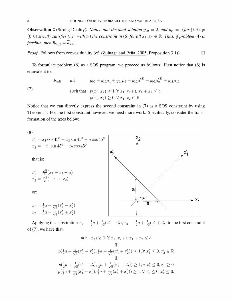
Notice that we can directly express the second constraint in (7) as a SOS constraint by usingTheorem 1. For the first constraint however, we need more work. Specifically, consider the trans-formation of the axes below:
(8)
x′1 = x1 cos 450 + x2 sin 450 − a cos 450
x′2 = −x1 sin 450 + x2 cos 450
that is:
x′1 =√
22
(x1 + x2 − a)
x′2 =√
22
(−x1 + x2)
or:
x1 = 12a+ 1√
2(x′1 − x′2)
x2 = 12a+ 1√
2(x′1 + x′2)
Applying the substitution x1 → 12a+ 1√
2(x′1−x′2), x2 → 1
2a+ 1√
2(x′1 +x′2) to the first constraint
of (7), we have that:
p(x1, x2) ≥ 1,∀ x1, x2 s.t. x1 + x2 ≤ a
mp(1
2a+ 1√
2(x′1 − x′2),
12a+ 1√
2(x′1 + x′2)) ≥ 1,∀ x′1 ≤ 0, x′2 ∈ Rm
p(12a+ 1√
2(x′1 − x′2),
12a+ 1√
2(x′1 + x′2)) ≥ 1,∀ x′1 ≤ 0, x′2 ≥ 0
p(12a+ 1√
2(x′1 − x′2),
12a+ 1√
2(x′1 + x′2)) ≥ 1,∀ x′1 ≤ 0, x′2 ≤ 0.
BOUNDS FOR RUIN PROBABILITIES AND VALUE AT RISK 9
By substituting x′1 → −x′1 in the second to last equation above and substituting x′1 → −x′1, x′2 →−x′2 in the last equation, we obtain that (7) is equivalent to:(9)dVaR = inf y00 + y10µ1 + y01µ2 + y20µ
(2)1 + y02µ
(2)2 + y11µ12
such that p(12a+ 1√
2(−x′1 − x′2),
12a+ 1√
2(−x′1 + x′2))− 1 ≥ 0,∀ x′1 ≥ 0, x′2 ≥ 0
p(12a+ 1√
2(−x′1 + x′2),
12a+ 1√
2(−x′1 − x′2))− 1 ≥ 0,∀ x′1 ≥ 0, x′2 ≥ 0.
p(x1, x2) ≥ 0, ∀ x1, x2 ∈ R.
To finish, from Theorem 2 (applied to the first two constraints of (9)) and Theorem 1 (applied tothe last constraint of (9)), it follows that (9) is equivalent to the following SOS program:
(10)dVaR = inf y00 + y10µ1 + y01µ2 + y20µ
(2)1 + y02µ
(2)2 + y11µ12
such that p(12a+ 1√
2(−x2
1 − x22),
12a+ 1√
2(−x2
1 + x22))− 1 is a SOS polynomial
p(12a+ 1√
2(−x2
1 + x22),
12a+ 1√
2(−x2
1 − x22))− 1 is a SOS polynomial
p(x21, x
22) is a SOS polynomial.
Notice that above we drop the primes in the variable labels (they are just variable labels). Also,we do not go through the details of q(x1, x2) = p(1
2a+ 1√
2(x1−x2),
12a+ 1√
2(x1 +x2))−1 and the
SOS constraint q(x21, x
22) = p(1
2a+ 1√
2(x2
1−x22),
12a+ 1√
2(x2
1 +x22))−1. The algebraic expressions
of the polynomials in (10) are left out for brevity purposes. In fact, with current SOS solvers it isnot even necessary to provide the expanded algebraic expression of these polynomials.
The SOS program (10) can be readily solved with a SOS programming solver. Thus, if prob-lem (4) is feasible (cf. Observation 1), it follows from Observation 2 that we can numericallyobtain the VaR semiparametric upper bound pVaR by solving problem (10) with a SOS solver.
3.1.2. Lower bound. We start with a semiparametric bound closely related to problem (5) as fol-lows:
(11)
pcVaR
:= sup Eπ(I{w1X1+w2X2≥a})
such that Eπ(1) = 1,
Eπ(Xi) = µi, i = 1, 2,
Eπ(X2i ) = µ
(2)i , i = 1, 2,
Eπ(X1X2) = µ12,
π a probability distribution in R2.
Notice that in (11) we are computing the upper semiparametric bound on the complement of theVaR probability Pr(w1X1+w2X2 ≥ a). Thus, it clearly follows that p
VaR= 1−pc
VaR(cf. (5)). The
10 BOUNDS FOR RUIN PROBABILITIES AND VALUE AT RISK
feasibility of problem (11) is also characterized by the moment matrix condition of Observation 1;and as it turns out, it is much easier to reformulate (11) as a SOS program.
As in previous sections, we begin by stating the dual of (11):
(12)dc
VaR = inf y00 + y10µ1 + y01µ2 + y20µ(2)1 + y02µ
(2)2 + y11µ12
such that p(x1, x2) ≥ I{x1+x2≥a},∀ x1, x2 ∈ R.
Analogous to Section 3.1.1 (see Observation 2), strong duality between (11) and (12) follows if(11) is feasibe (i.e., if the condition in Observation 1 is satisfied).
Following the analogous steps to those taken in Section 3.1.1 for problem (6), we obtain thatproblem (12) is equivalent to the SOS program below:
(13)
dcVaR = inf y00 + y10µ1 + y01µ2 + y20µ
(2)1 + y02µ
(2)2 + y11µ12
such that p(12a+ 1√
2(x2
1 − x22),
12a+ 1√
2(x2
1 + x22))− 1 is a SOS polynomial
p(12a+ 1√
2(x2
1 + x22),
12a+ 1√
2(x2
1 − x22))− 1 is a SOS polynomial
p(x21, x
22) is a SOS polynomial.
The SOS program (13) can be readily solved with a SOS programming solver. Thus, if prob-lem (5) is feasible (cf. Observation 1), it follows that we can numerically obtain the VaR semipara-metric lower bound p
VaR= 1− dc
VaR by solving problem (13) with a SOS solver.It follows the probability Pr(X1 + X2 ≤ a) = 1 − Pr(X1 + X2 ≥ a). As long as we know
the upper and lower bounds on Pr(X1 + X2 ≥ a), the bounds Pr(X1 + X2 ≤ a) can be easilyobtained.
3.2. Probability Bounds. We consider the problem of finding sharp upper and lower bounds onthe probability Pr(X1 ≤ t1 and X2 ≤ t2) of two non-negative random variables X1, X2, attainingvalues lower than or equal to t1, t2 ∈ R+ respectively, without making any assumption on thedistribution of the random variables X1, X2. Finding the sharp upper and lower semiparametricbounds for this problem can be obtained by setting problem (2) as φ(X1, X2) = I{X1≤t1 and X2≤t2}
andD = R+2 (cf. Section 2), given up to the second order moment information (means, variances,and covariance) on X1, X2:
(14)
p := sup Eπ(I{X1≤t1 and X2≤t2})
such that Eπ(1) = 1,
Eπ(Xi) = µi, i = 1, 2,
Eπ(X2i ) = µ
(2)i , i = 1, 2,
Eπ(X1X2) = µ12,
π a probability distribution in R+2,
BOUNDS FOR RUIN PROBABILITIES AND VALUE AT RISK 11
and
(15)
p := inf Eπ(I{X1≤t1 and X2≤t2})
such that Eπ(1) = 1,
Eπ(Xi) = µi, i = 1, 2,
Eπ(X2i ) = µ
(2)i , i = 1, 2,
Eπ(X1X2) = µ12,
π a probability distribution in R+2.
Before obtaining the SOS programming formulation of these problems, we discuss their feasibilityin terms of the moment information.
Observation 3 (Feasibility). Problems (14) and (15) are feasible if and only if Σ is a positivesemidefinite matrix (i.e., all eigenvalues are greater than or equal to zero) and all elements of Σ
are non-negative, where Σ is the moment matrix:
Σ =
1 µ1 µ2
µ1 µ(2)1 µ12
µ2 µ12 µ(2)2
.Next we derive SOS programs to numerically compute p, and p by using SOS programming
solvers.
3.2.1. Upper bound. We begin by stating the dual problem of (14):
(16)d = inf y00 + y10µ1 + y01µ2 + y20µ
(2)1 + y02µ
(2)2 + y11µ12
such that p(x1, x2) ≥ I{x1≤t1 and x2≤t2},∀ x1, x2 ≥ 0.
As the following observation states, as long as problem (14) is feasible, we can obtain p bysolving problem (16).
Observation 4 (Strong Duality). Notice that the dual solution y00 = 2, and yij = 0 for (i, j) 6=(0, 0) strictly satisfies (i.e., with >) the constraint in (16) for all x1, x2 ≥ 0. Thus, if problem (14)is feasible, then p = d.
Proof. Follows from convex duality (cf. (Zuluaga and Pena, 2005, Proposition 3.1)). �
To formulate problem (16) as a SOS program, we proceed as follows. First notice that (16) isequivalent to:
(17)
d = inf y00 + y10µ1 + y01µ2 + y20µ(2)1 + y02µ
(2)2 + y11µ12
such that p(x1, x2) ≥ 1,∀ 0 ≤ x1 ≤ t1, 0 ≤ x2 ≤ t2
p(x1, x2) ≥ 0,∀ x1, x2 ≥ 0.
12 BOUNDS FOR RUIN PROBABILITIES AND VALUE AT RISK
Although the second constraint of (17) can be handled directly, the first constraint is difficultto reformulate as a SOS constraint. That is, there is no linear transformation from 0 ≤ x1 ≤t1, 0 ≤ x2 ≤ t2 to R+2 or to R2 (that would allow the use of Theorems 1 and 2). Thus, wechange the problem to end up with a SOS program that either solves or approximates problem (17).Specifically, consider the following problem related to (17):
(18)
d′= inf y00 + y10µ1 + y01µ2 + y20µ
(2)1 + y02µ
(2)2 + y11µ12
such that p(x1, x2) ≥ 1,∀ x1 ≤ t1, x2 ≤ t2
p(x1, x2) ≥ 0,∀ x1 ≥ 0, x2 ≥ 0.
Notice that (18) is less constrained than (17) (the first constraint of (18) includes more valuesof x1 and x2). Thus, d
′is a upper bound on d; that is d
′ ≥ d (in fact, our intuition suggests thatd′= d).After we apply the substitution x1 → t1 − x1, x2 → t2 − x2 to the first constraint of (18),
problem (18) is equivalent to:
(19)
d′= inf y00 + y10µ1 + y01µ2 + y20µ
(2)1 + y02µ
(2)2 + y11µ12
such that p(t1 − x1, t2 − x2)− 1 ≥ 0, ∀ x1, x2 ≥ 0
p(x1, x2) ≥ 0, ∀ x1, x2 ≥ 0.
If we let q(x1, x2) = p(t1 − x1, t2 − x2)− 1, i.e.
q(x1, x2) = (y00 + y10t1 + y01t2 + y20t21 + y02t
22 + y11t1t2 − 1)
−(y10 + 2t1y20 + y11t2)x1
−(y01 + 2t2y02 + y11t1)x2
+y20x21 + y02x
22 + y11x1x2.
The first constraint of (19) can be replaced by q(x1, x2) ≥ 0,∀ x1, x2 ≥ 0. To finish, fromTheorem 2, it follows that (19) (with the first constraint written in terms of q(x1, x2)) is equivalentto the following SOS program:
(20)
d′= inf y00 + y10µ1 + y01µ2 + y20µ
(2)1 + y02µ
(2)2 + y11µ12
such that q(x21, x
22) is a SOS polynomial
p(x21, x
22) is a SOS polynomial.
The SOS program (20) can be readily solved with a SOS programming solver. Thus, if prob-lem (14) is feasible (cf. Observation 3), it follows from Observation 4 that we can numericallyobtain a semiparametric bound Pr(X1 ≤ t1, X2 ≤ t2) ≤ d
′by solving problem (20) with a SOS
solver.
BOUNDS FOR RUIN PROBABILITIES AND VALUE AT RISK 13
3.2.2. Lower bound. We begin with stating the dual problem of (15):
(21)d = sup y00 + y10µ1 + y01µ2 + y20µ
(2)1 + y02µ
(2)2 + y11µ12
such that p(x1, x2) ≤ I{x1≤t1 and x2≤t2},∀ x1, x2 ≥ 0.
As the following observation states, as long as problem (15) is feasible, we can obtain p bysolving problem (21).
Observation 5 (Strong Duality). Notice that the dual solution y00 = −1, and yij = 0 for (i, j) 6=(0, 0) strictly satisfies (i.e., with <) the constraint in (21) for all x1, x2 ≥ 0. Thus, if problem (15)is feasible, then p = d.
Proof. Follows from convex duality (cf. (Zuluaga and Pena, 2005, Proposition 3.1)). �
Now, problem (21) is equivalent to
(22)
d = sup y00 + y10µ1 + y01µ2 + y20µ(2)1 + y02µ
(2)2 + y11µ12
such that p(x1, x2) ≤ 1,∀ 0 ≤ x1 ≤ t1, 0 ≤ x2 ≤ t2
p(x1, x2) ≤ 0, ∀ x1 ≥ t1, x2 ≥ 0,
p(x1, x2) ≤ 0, ∀ x1 ≥ 0, x2 ≥ t2.
Using the similar approximation as the upper bound to the first constraint and applying x1 →t1 + x1, x2 → t2 + x2 to the second and third constraints respectively, we have that (22) can beapproximated by solving:
(23)
d′ = sup y00 + y10µ1 + y01µ2 + y20µ(2)1 + y02µ
(2)2 + y11µ12
such that 1− p(t1 − x1, t2 − x2) ≥ 0,∀ x1, x2 ≥ 0
−p(t1 + x1, x2) ≥ 0, ∀ x1, x2 ≥ 0,
−p(x1, t2 + x2) ≥ 0, ∀ x1, x2 ≥ 0,
where d′ ≤ d. Similar to the upper bound problem, we now let:
q1(x1, x2) = 1− p(t1 − x1, t2 − x2)
q2(x1, x2) = −p(t1 + x1, x2)
q3(x1, x2) = −p(x1, t2 + x2);
14 BOUNDS FOR RUIN PROBABILITIES AND VALUE AT RISK
that is,q1(x1, x2) = 1− (y00 + y10t1 + y01t2 + y20t
21 + y02t
22 + y11t1t2)
+(y10 + 2t1y20 + y11t2)x1 + (y01 + 2t2y02 + y11t1)x2
−y20x21 − y02x
22 − y11x1x2
q2(x1, x2) = −(y00 + y10t1 + y20t21)
−(y10 + 2y20t1)x1 − (y01 + y11t1)x2
−y20x21 − y02x
22 − y11x1x2
q3(x1, x2) = −(y00 + y01t2 + y02t22)
−(y10 + y11t2)x1 − (y01 + 2y02t2)x2
−y20x21 − y02x
22 − y11x1x2.
To finish, from Theorem 2, it follows that (23) (with the three constraints written in terms ofqi(x1, x2), i = 1, 2, 3) is equivalent to the following SOS program:
(24)
d′ = sup y00 + y10µ1 + y01µ2 + y20µ(2)1 + y02µ
(2)2 + y11µ12
such that q1(x21, x
22) is a SOS polynomial
q2(x21, x
22) is a SOS polynomial
q3(x21, x
22) is a SOS polynomial.
The SOS program (24) can be readily solved with a SOS programming solver. Thus, if prob-lem (15) is feasible (cf. Observation 3), it follows from Observation 5 that we can numericallyapproximate the ruin probability semiparametric lower bound d by solving problem (24) with aSOS solver. Furthermore, notice that by solving (20) and (24) we obtain a “100% confidence in-terval” d′ ≤ Pr(X1 ≤ t1 and X2 ≤ t2) ≤ d
′on the value of the probability when given only up to
the second order moment information on the non-negative random variables X1, X2.Following the same technique, we also derive the upper and lower bounds on the joint probability
Pr(X1 ≥ t1 and X2 ≥ t2) of two non-negative random variables X1, X2. See Appendix A fordetails.
3.3. Bounds on Stop-Loss payments. Stop-loss payments we consider here have two loss com-ponents X1 and X2. For example, a homeowner’s policy covers both property losses X1 and liabil-ity lossesX2. Similarly, X1 could be hospital room and board costs andX2 be surgical expenses inhealth insurance. We find the upper and lower bounds on the aggregate loss Z = X1 +X2, giventhe mean, variance and covariance of X1 and X2. This time our function φ(X1, X2) in problem (2)is defined as follows:
(25) φ(X1, X2) =
b if X1 +X2 ≥ a+ b
X1 +X2 − a if a ≤ X1 +X2 ≤ a+ b
0 if X1 +X2 ≤ a.
BOUNDS FOR RUIN PROBABILITIES AND VALUE AT RISK 15
Suppose the function φ(X1, X2) represents the benefits a direct insurer pays to a reinsurer, givenlosses of X1 and X2. Under this contract, when the total losses are less than a, the direct insurerretains all losses. When the sum exceeds the threshold a, the reinsurer pays the excess up to amaximum of b. If the total losses exceed a + b, the part higher than b will be retained or ceded toother reinsurers by the direct insurer. Compared with the previous problems, bounds on stop-losscoverage is relatively easy to compute since X1 and X2 always appear in the form of X1 +X2 inthe objective function (25). Therefore, this problem can be considered as a one variable problemby setting Z = X1 +X2 and calculating the moments of Z as follows:
µz = µ1 + µ2 and µ(2)z = µ
(2)1 + µ
(2)2 + 2µ12.
With this transformation, the objective function (25) can be written as:
(26) φ(Z) =
b if Z ≥ a+ b
Z − a if a ≤ Z ≤ a+ b
0 if Z ≤ a.
Cox (1991) provides an explicit solution to a transformed problem of (26).1 We first solve thisproblem numerically with a SOS program and then compare its results with those obtained fromCox (1991)’s method to test the robustness of the SOS approach.
3.3.1. SOS program. Given problem (25) and D = R+2, the upper and lower semiparametricbounds for this problem are formulated as the following optimization problems:2
(27)
pStopLoss(or pStopLoss
) = sup (or inf) Eπ(φ(X1 +X2))
such that Eπ(1) = 1,
Eπ(Xi) = µi, i = 1, 2,
Eπ(X2i ) = µ
(2)i , i = 1, 2,
Eπ(X1X2) = µ12,
π a probability distribution in R+2.
1Only few bound problems have explicit solutions, but many of them can be solved by SOS programs.2In general, this problem has a support D = R2. But if X1 and X2 stand for losses (as in our example), they arenonnegative numbers.
16 BOUNDS FOR RUIN PROBABILITIES AND VALUE AT RISK
Letting Z = X1 + X2, problem (27) is transferred to a one-variable bound problem. Its upperbound is expressed as:
(28)
pStopLoss = sup Eπ(φ(Z))
such that Eπ(1) = 1,
Eπ(Z) = µz
Eπ(Z2) = µ(2)z
π a probability distribution in R+,
and its lower bound is as follows:
(29)
pStopLoss
= inf Eπ(φ(Z))
such that Eπ(1) = 1,
Eπ(Z) = µz
Eπ(Z2) = µ(2)z
π a probability distribution in R+.
Before obtaining the SOS programming formulation of the primal problems (28) and (29), wediscuss their feasibility in terms of their moment parameters.
Observation 6 (Feasibility). When the feasibility of stop-loss bounds is considered, we shouldgo back to the two-variable problem with the moment matrix Σ expressed as follows. Similar toprobability bounds problem in Section 3.2, problems (28) and (29) are feasible if and only if Σ is apositive semidefinite matrix (i.e., all eigenvalues are greater than or equal to zero) and all elementsof Σ are non-negative.
Σ =
1 µ1 µ2
µ1 µ(2)1 µ12
µ2 µ12 µ(2)2
.Furthermore, when two-variable feasibility is satisfied, one-variable feasibility is also met auto-matically. That is, Σz is a positive semidefinite matrix and all elements of Σz are non-negative.
Σz =
[1 µz
µz µ(2)z
].
Next we derive SOS programs to numerically compute pStopLoss, and pStopLoss
by using SOSprogramming solvers.
Upper bound. We begin with stating the dual problem of (28) as follows:
(30)dStoploss = inf y0 + y1µz + y2µ
(2)z
such that p(z) ≥ φ(z),∀ z ≥ 0,
where p(z) = y0 + y1z + y2z2.
BOUNDS FOR RUIN PROBABILITIES AND VALUE AT RISK 17
As the following observation states, as long as problem (28) is feasible, we can obtain pStoploss
by solving problem (30).
Observation 7 (Strong Duality). Notice that the dual solution y0 = 2, and y1 = y2 = 0 strictlysatisfies (i.e., with >) the constraint in (30) for all z ≥ 0. Thus, if problem (28) is feasible, thenpStoploss = dStoploss.
Proof. Follows from convex duality (cf. (Zuluaga and Pena, 2005, Proposition 3.1)). �
To formulate problem (30) as a SOS program, we rewrite the inequality constraint in (30) asthree simultaneous inequalities. Problem (30) is equivalent to:
(31)
dStopLoss = inf y0 + y1µz + y2µ(2)z
such that p(z)− b ≥ 0, ∀z ∈ [a+ b,∞)
p(z)− z + a ≥ 0, ∀z ∈ [a, a+ b]
p(z) ≥ 0, ∀z ∈ [0, a].
The univariate SOS program (31) can be readily solved with a SOS programming solver. Thus, ifproblem (28) is feasible (cf. Observation 6), it follows from Observation 7 that we can numericallyobtain the semiparametric upper bound pStoploss by solving problem (31) with a SOS solver.
Lower bound. We begin with staring the dual problem of (29):
(32)dStoploss = sup y0 + y1µz + y2µ
(2)z
such that p(z) ≤ φ(z),∀ z ≥ 0.
As the following observation states, as long as problem (29) is feasible, we can obtain pStoploss
by solving problem (32).
Observation 8 (Strong Duality). Notice that the dual solution y0 = −1, and y1 = y2 = 0 strictlysatisfies (i.e., with >) the constraint in (32) for all z ≥ 0. Thus, if problem (29) is feasible, thenp
Stoploss= dStoploss.
Proof. Follows from convex duality (cf. (Zuluaga and Pena, 2005, Proposition 3.1)). �
To formulate problem (32) as a SOS program, we rewrite the inequality constraint in (32) asthree simultaneous inequalities. Problem (32) is equivalent to:
(33)
dStopLoss = sup y0 + y1µz + y2µ(2)z
such that b− p(z) ≥ 0, ∀z ∈ [a+ b,∞)
(z − a)− p(z) ≥ 0, ∀z ∈ [a, a+ b]
−p(z) ≥ 0, ∀z ∈ [0, a].
18 BOUNDS FOR RUIN PROBABILITIES AND VALUE AT RISK
The univariate SOS program (33) can be readily solved with a SOS programming solver. Thus, ifproblem (29) is feasible (cf. Observation 6), it follows from Observation 8 that we can numericallyobtain the semiparametric lower bound p
Stoplossby solving problem (33) with a SOS solver.
In addition, the lower bound of stop-loss payment p(φ) can be obtained by solving upper boundof a transformed problem with objective function ψ(Z) where ψ(Z) = Z − φ(Z).
(34) ψ(Z) =
Z − b if Z ≥ a+ b
a if a ≤ Z ≤ a+ b
Z if Z ≤ a.
If the moment matrix Σ satisfies the feasibility requirement (cf. Observation 6), we can numeri-cally obtain the semiparametric upper bound p(ψ) by solving the following dual problem (35) witha SOS solver:
(35)
d(ψ) = inf y0 + y1µz + y2µ(2)z
such that p(z)− (z − b) ≥ 0, ∀z ∈ [a+ b,∞)
p(z)− a ≥ 0, ∀z ∈ [a, a+ b]
p(z)− z ≥ 0, ∀z ∈ [0, a].
Apparently, the upper bound of ψ(Z), p(ψ) = sup{Eπ[ψ(Z)]} given the same moment informa-tion, equals µz minus the lower bound of φ(Z). That is, p(ψ) = µz − p(φ). Similarly, the upperbound of stop-loss payment p(φ) can be obtained from the relation p(ψ) = µz − p(φ) after wesolve p(ψ).
Proof. See Appendix B. �
3.3.2. Cox (1991)’s Method. Suppose a direct insurer purchases a reinsurance policy and his over-all claim payment ψ(Z) follows equation (34). Cox (1991) develops an explicit solution to thebounds of the expected claim payment E[ψ(Z)] of the direct insurer, given mean and variance.p(ψ), the upper bound on E[ψ(Z)], is described as follows: For values of a satisfying 0 ≤ a < µz,
p(ψ) =
(µz − b)(µz − a)2 + µzσ
2z
(µz − a)2 + σ2z
if a ≤ a+ b ≤ σ2z + µ2
z − a2
2(µz − a)
a+1
2
[µz − a− b+
√(a+ b− µz)2 + σ2
z
]if a+ b >
σ2z + µ2
z − a2
2(µz − a),
where σz =
õ
(2)z − µ2
z.
When a ≥ µz, the upper bound p(ψ) = µz.The lower bound on E[ψ(Z)], p(ψ), is described as follows: For values of a + b satisfying
0 ≤ a+ b ≤ µz,p(ψ) = µz − b.
BOUNDS FOR RUIN PROBABILITIES AND VALUE AT RISK 19
If µz ≤ a+ b ≤ µz +σ2
z
µz
,
p(ψ) =aµz
a+ b.
When a+ b ≥ µz +σ2
z
µz
,
p(ψ) =
aµ2z
σ2z + µ2
z
if 0 ≤ a ≤ µz
2+
σ2z
2µz
1
2
[µz + a−
√(µz − a)2 + σ2
z
]ifµz
2+
σ2z
2µz
< a ≤ (a+ b)2 − µ2z − σ2
z
2(a+ b− µz)µz(a+ b− µz)
2 + (µz − b)σ2z
(a+ b− µz)2 + σ2z
if(a+ b)2 − µ2
z − σ2z
2(a+ b− µz)≤ a ≤ a+ b.
After the upper and lower bounds p(ψ) and p(ψ) are calculated, the bounds on the stop-losspayment φ(Z) = Z−ψ(Z) can be found by the relations p(φ) = µz−p(ψ) and p(φ) = µz−p(ψ).
4. NUMERICAL ANALYSIS
To understand the extent to which extreme events affect our decision, we apply the momentmethods to the insurance and financial markets with three examples. The first example is an ap-plication of VaR probability bounds we derive in Section 3.1; the second one is for probabilitybounds (See Section 3.2); the bounds on stop-loss payments derived in Section 3.3 are illustratedin example three.
4.1. Example of VaR Probability Bounds. The VaR problem is to find the upper and lowerbounds on a where Pr(w1X1 + w2X2 ≤ a) = 0.05, subject to the moment information on X1 andX2. We connect this to a semiparametric probability problem by finding bounds on Pr(w1X1 +
w2X2 ≤ a) for enough values of a to solve the inverse problem.In Section 3.1, we find bounds for the special case Pr(X1 + X2 ≤ a). We can easily convert
Pr(w1X1 + w2X2 ≤ a) to Pr(X1 + X2 ≤ a) by adjusting the moments of X1 and X2. LetX
′1 = w1X1 and X ′
2 = w2X2. Then we have the following relationships:
(36)
E(X′i) = E(wiXi) = wiµi, i = 1, 2
E(X′2i ) = E(w2
iX2i ) = w2
i µ(2)i , i = 1, 2
E(X′1X
′2) = E(w1X1w2X2) = w1w2µ12.
That is, we can rescale a problem in the form w1X1 + w2X2 ≤ a to the form X1 +X2 ≤ a.To show how to solve the bound on VaR, we study a possible extreme scenario in the interna-
tional stock markets. That is, what may happen if the stock indices of two countries both reachsome very low levels. Specifically, we analyze the tail joint probability of total return of a portfolioinvesting in the S&P500 and Nikkei indices.
20 BOUNDS FOR RUIN PROBABILITIES AND VALUE AT RISK
First, we calculate the moments of the S&P500 annualized return (denoted rsp) and that of theNikkei (denoted rnk) based on the monthly historical data from 1984 to 2006. There are 276observations in our sample. Their moments are as follows:
E(X1) = 0.1107 = E(rsp) = µ1 E(X21 ) = 0.0349
E(X2) = 0.0473 = E(rnk) = µ2 E(X22 ) = 0.0554
Var(X1) = 0.0227 = Var(rsp) ρ = 0.4190
Var(X2) = 0.0531 = Var(rnk)
Cov(X1, X2) = 0.0145 = Cov(rsp, rnk).
On average, the S&P500 annualized return (0.1107) is higher than that of Nikkei (0.0473) but theS&P500 is less volatile (Var(rsp) < Var(rnk)). Moreover, they have a positive correlation 0.4190.This relatively high correlation reflects the impact of economic globalization, thus weakening thediversification effect.
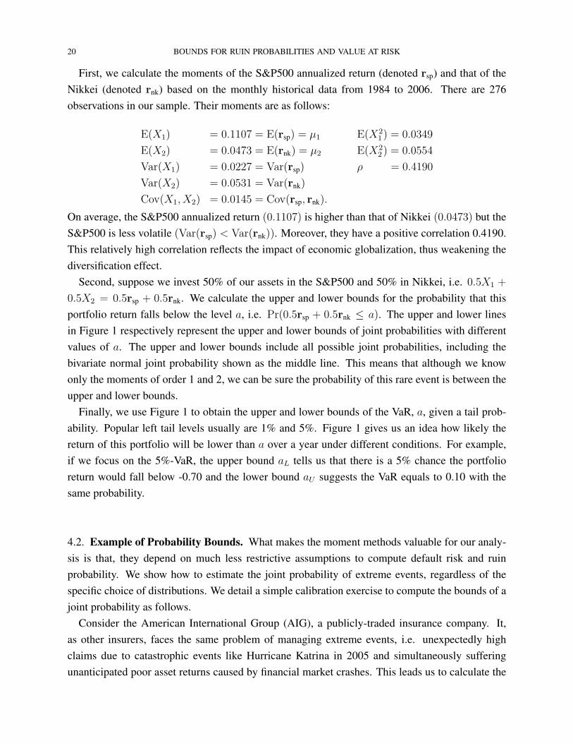
Second, suppose we invest 50% of our assets in the S&P500 and 50% in Nikkei, i.e. 0.5X1 +
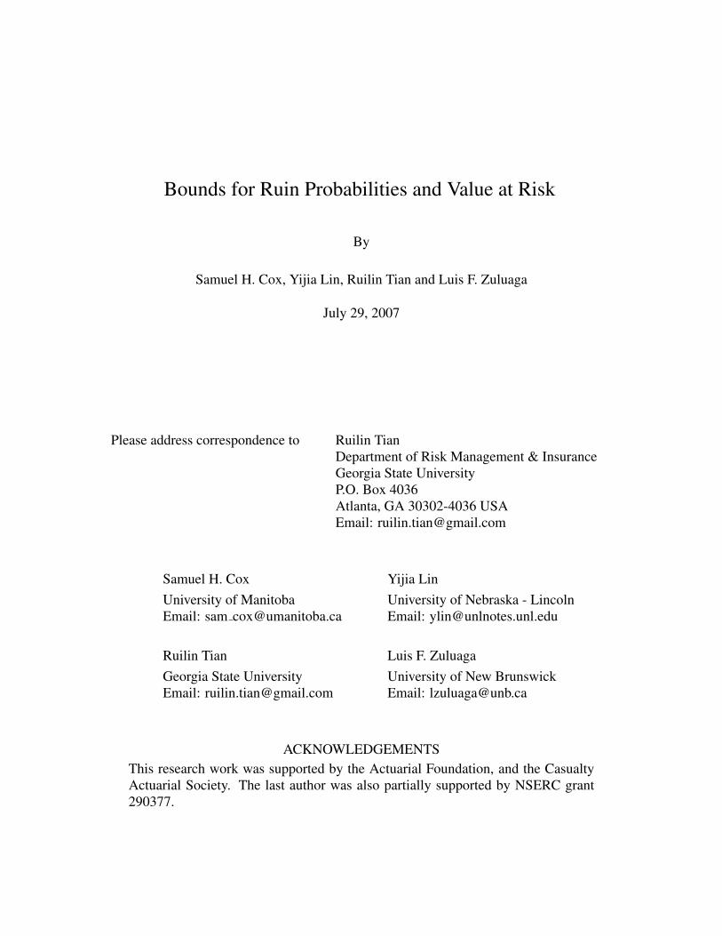
0.5X2 = 0.5rsp + 0.5rnk. We calculate the upper and lower bounds for the probability that thisportfolio return falls below the level a, i.e. Pr(0.5rsp + 0.5rnk ≤ a). The upper and lower linesin Figure 1 respectively represent the upper and lower bounds of joint probabilities with differentvalues of a. The upper and lower bounds include all possible joint probabilities, including thebivariate normal joint probability shown as the middle line. This means that although we knowonly the moments of order 1 and 2, we can be sure the probability of this rare event is between theupper and lower bounds.
Finally, we use Figure 1 to obtain the upper and lower bounds of the VaR, a, given a tail prob-ability. Popular left tail levels usually are 1% and 5%. Figure 1 gives us an idea how likely thereturn of this portfolio will be lower than a over a year under different conditions. For example,if we focus on the 5%-VaR, the upper bound aL tells us that there is a 5% chance the portfolioreturn would fall below -0.70 and the lower bound aU suggests the VaR equals to 0.10 with thesame probability.
4.2. Example of Probability Bounds. What makes the moment methods valuable for our analy-sis is that, they depend on much less restrictive assumptions to compute default risk and ruinprobability. We show how to estimate the joint probability of extreme events, regardless of thespecific choice of distributions. We detail a simple calibration exercise to compute the bounds of ajoint probability as follows.
Consider the American International Group (AIG), a publicly-traded insurance company. It,as other insurers, faces the same problem of managing extreme events, i.e. unexpectedly highclaims due to catastrophic events like Hurricane Katrina in 2005 and simultaneously sufferingunanticipated poor asset returns caused by financial market crashes. This leads us to calculate the
BOUNDS FOR RUIN PROBABILITIES AND VALUE AT RISK 21
FIGURE 1. Upper and lower bounds for the probability Pr(0.5rsp + 0.5rnk ≤ a)where rsp is the monthly annualized return on the S&P500 index and rnk is thatof the Nikkei index. The vertical axis is the probability and the horizontal axisstands for different values of a. The 5% VaR0.05 of the normal distribution equals toa = −0.20. It falls between the semiparametric lower bound aL and upper boundaU . That is, aL < VaR0.05 < aU .
bounds on Pr(r ≤ t1,m ≤ t2) given moment information, where r is AIG’s return on its investedassets and m is the margin on its insurance business.
The return ri of asset i in the portfolio is equal to Pi,t/Pi,t−1 − 1 where Pi,t−1 and Pi,t denotethe prices of asset i at the beginning and the end of the period. If we focus on the price ratio, thecondition r ≤ t1 changes to
(37) X1i = ri + 1 =Pi,t
Pi,t−1
≤ t′1,
where t′1 = t1 + 1. As for AIG’s portfolio, r is the weighted average return of 6 assets: stocks,government bonds, corporate bonds, real estates, mortgages and cash & short-term investments(i = 1, 2, . . . , 6):
r =6∑
i=1
wiX1i − 1 = X1 − 1,
where wi is the weight of asset i in the portfolio. Indeed, we calculate the bounds for Pr(X1 ≤t′1) = Pr(
∑6i=1wiX1i ≤ t′1) which is equivalent to Pr(r ≤ t1). We make this shift from asset
returns to price ratios to apply our SOS results because we need non-negative random variables.
22 BOUNDS FOR RUIN PROBABILITIES AND VALUE AT RISK
The margin on insurance business m is defined as
m = 1− LR,
where LR is the economic loss ratio. Following a standard measure in the insurance literature(Cummins, 1990; Phillips, Cummins, and Allen, 1998; Yu and Lin, 2007), we calculate the eco-nomic loss ratio as follows:
LR =
∑12k=1 PVFk × NLIk∑12
k=1 NPEk
.
We classify AIG’s business into twelve categories (k = 1, 2, . . . , 12).3 The present value factorPVFk is calculated from the industry liability payout factor for loss category k (k = 1, 2, . . . , 12)and the discount rates. The discount rates are the risk-free rates estimated from the U.S. Treasuryspot-rate yield curves.4 The variable NLIk is the net loss incurred for category k for AIG. Thevariable NPEk is its net premium earned for category k. See Cummins (1990) for calculationdetails. Using the actual premium in the denominator and the riskless present value of losses inthe numerator allows us to capture changes in loss ratios due to insurance shocks. In order toreformulate the condition m ≤ t2 so that the condition fits our SOS results, similar to the assetreturn case, we replace m ≤ t2 withX2 ≤ t′2 whereX2 = m+1 and t′2 = t2 +1. It clearly followsthat Pr(m ≤ t2) is equivalent to Pr(X2 ≤ t′2).
The weights of different asset categories (wi) are calculated from the quarterly data of the Na-tional Association of Insurance Commissioners (NAIC). The quarterly AIG and industry lossesand premiums are also obtained from the NAIC. We use the quarterly annualized returns of theStandard & Poor’s 500 (S&P500), the LB IT government bond index, the domestic high-yieldcorporate bond index, the NAREIT-All index, the ML mortgage index and the U.S. 30 Day T-Billas proxies for AIG’s stock returns, government bond returns, corporate bond returns, real estatereturns, mortgage returns and cash & short-term investment returns respectively. In sum, we have52 quarterly observations from 1991 to 2003. Here are their moments:
E(X1) = 1.0442 = E(r) + 1 = µ1 E(X21 ) = 1.0967
E(X2) = 1.3393 = E(m) + 1 = µ2 E(X22 ) = 1.8287
Var(X1) = 0.0063 = Var(r) ρ = 0.1244
Var(X2) = 0.0350 = Var(m)
Cov(X1, X2) = 0.0019.
On average, AIG’s margin on its insurance business (E(m) = 0.3393) is higher than its assetreturn (E(r) = 0.0442) while the margin is more volatile (Var(m) > Var(r)). Moreover, the asset
3Following the NAIC classifications, our twelve insurance business categories include farmowners and homeownersmultiple peril; private passenger auto liability; workers’ compensation; commercial multiple peril; medical malprac-tice; special liability; special property; automobile physical damage; fidelity and surety; other; financial guarantee andmortgage guarantee; and other liability and product liability.4Data source: the Federal Reserve Bank of St. Louis’ Federal Reserve Economic Data (FRED).
BOUNDS FOR RUIN PROBABILITIES AND VALUE AT RISK 23
return and insurance margin are positively correlated (0.1244). This implies that generally AIG’sinsurance business and investment performances moderately move in the same direction.
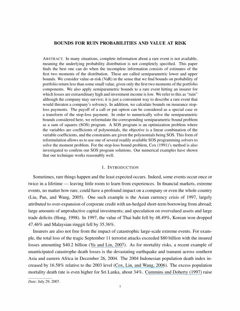
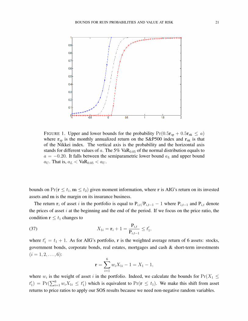
FIGURE 2. The upper left plot shows the upper bound of the joint probabilityPr(r ≤ t1,m ≤ t2) where r is invested asset return and m is insurance businessmargin of AIG. The upper right one is the bivariate normal cumulative probabilitieswith the same moments for AIG. The ratio of the upper bound to the bivariate nor-mal cumulative joint probabilities is shown in the third graph. The vertical axis ofthe graphs is the probability. It is the ratio in the third graph. The two axes at thebottom in all three graphs represent the return t1 and the insurance margin t2.
To examine the tail-risk implication of our model, we start with the SOS programming to solvePr(r ≤ t1,m ≤ t2). Then we compare it to the bivariate normal cumulative joint probability withthe same set of moments. The upper left 3-dimensional (3D) plot in Figure 2 shows the upperbounds of the joint probability Pr(r ≤ t1,m ≤ t2) with different values of t1 and t2 and the upperright one is the bivariate normal cumulative joint probabilities with the same moments for AIG.The lower bound is always zero. The ratios of the upper bounds to the bivariate normal cumulativejoint probabilities are shown in the third graph. We can see that the ratios are always above 1.This means that the upper bound probabilities are always higher than those of the bivariate normal.Their difference is much larger when t1 and t2 are low. For example, when t1 = 0 and t2 = 0, theupper bound of Pr(r ≤ 0,m ≤ 0) is about 45 times higher than the cumulative joint probabilityof the bivariate normal. That is, the upper bound has a much fatter tail.
Next, we explore the upper bound implication for the joint probabilities across different valuesof one ti given the other tj is unchanged (i = 1 or 2 and i 6= j). Specifically, we are interestedin how one value (e.g. asset return t1) changes the joint tail probability if the other value (e.g.
24 BOUNDS FOR RUIN PROBABILITIES AND VALUE AT RISK
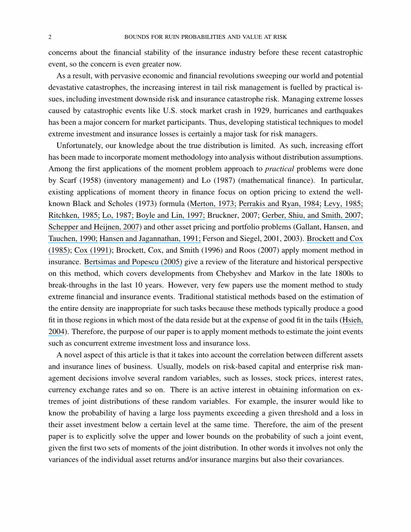
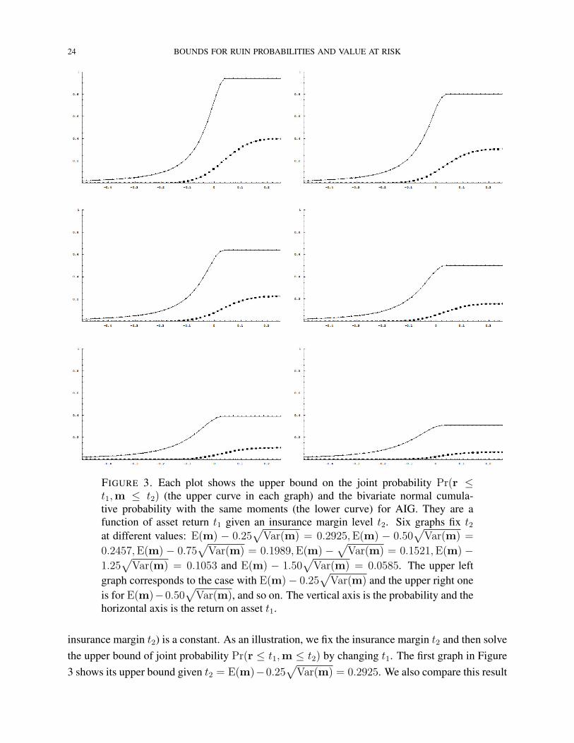
FIGURE 3. Each plot shows the upper bound on the joint probability Pr(r ≤t1,m ≤ t2) (the upper curve in each graph) and the bivariate normal cumula-tive probability with the same moments (the lower curve) for AIG. They are afunction of asset return t1 given an insurance margin level t2. Six graphs fix t2at different values: E(m) − 0.25
√Var(m) = 0.2925,E(m) − 0.50
√Var(m) =
0.2457,E(m) − 0.75√
Var(m) = 0.1989,E(m) −√
Var(m) = 0.1521,E(m) −1.25
√Var(m) = 0.1053 and E(m) − 1.50
√Var(m) = 0.0585. The upper left
graph corresponds to the case with E(m)− 0.25√
Var(m) and the upper right oneis for E(m)−0.50
√Var(m), and so on. The vertical axis is the probability and the
horizontal axis is the return on asset t1.
insurance margin t2) is a constant. As an illustration, we fix the insurance margin t2 and then solvethe upper bound of joint probability Pr(r ≤ t1,m ≤ t2) by changing t1. The first graph in Figure3 shows its upper bound given t2 = E(m)−0.25
√Var(m) = 0.2925. We also compare this result
BOUNDS FOR RUIN PROBABILITIES AND VALUE AT RISK 25
with the bivariate normal case. As we expect, the upper bound is above the bivariate normal curve.That is, the upper bound has a fatter tail which suggests a higher ruin probability.
Furthermore, we set the variable t2 (insurance margin) at five different levels based on 0.5, 0.75,1, 1.25 and 1.50 standard deviations lower than the mean: 0.2457, 0.1989, 0.1521, 0.1053 and0.0585. Then we draw their upper bounds and bivariate normal curves (the last five graphs inFigure 3). The trend of these graphs are consistent with our expectation. As t2 decreases, thecumulative joint probability levels out at a lower value. For example, when t2 = 0.2925, the upperbound of cumulative joint probability stays at 0.95 after it reaches this level. However, the stablelevel is only about 0.35 when t2 = 0.0585. Intuitively, a lower value is associated with a lowercumulative probability. Again, the bivariate normal curve is below the upper bound in all graphs.
4.3. Example of Stop-loss Payments. In this section, we find the upper and lower bounds on theexpected payment of a stop-loss contract written by a reinsurance company. Suppose AIG sells$1 million new homeowners insurance and $1 million new private passenger auto liability policiesthis year. It reinsures claim costs in excess of a million arising from these two businesses to SwissRe. Swiss Re pays part of AIG’s claims only if the threshold or deductible a is reached, subjectto a policy limit b million. The upper and lower bounds on the expected payment of Swiss Re isexamined here following Section 3.3.
The quarterly data of AIG from 1991 to 2004 are obtained from the NAIC. There are 56 ob-servations from which we calculate the moments of AIG loss payments per $1 million premiumearned, respectively, for its homeowners insurance (LHO) and its private passenger auto liabilityinsurance (LPPA). Their moments of loss amounts in million dollars are summarized as follows:
E(X1) = 0.6370 = E(LHO) = µ1 E(X21 ) = 0.9364
E(X2) = 0.6844 = E(LPPA) = µ2 E(X22 ) = 0.5073
Var(X1) = 0.5306 = Var(LHO) ρ = 0.1647
Var(X2) = 0.0390 = Var(LPPA)
Cov(X1, X2) = 0.02369.
On average, the expected claim payments of these two lines of business are similar although thehomeowners insurance is much more volatile since the homeowners business is more vulnerableto catastrophes and other weather-related claims.
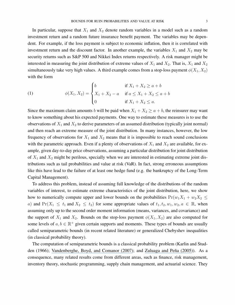
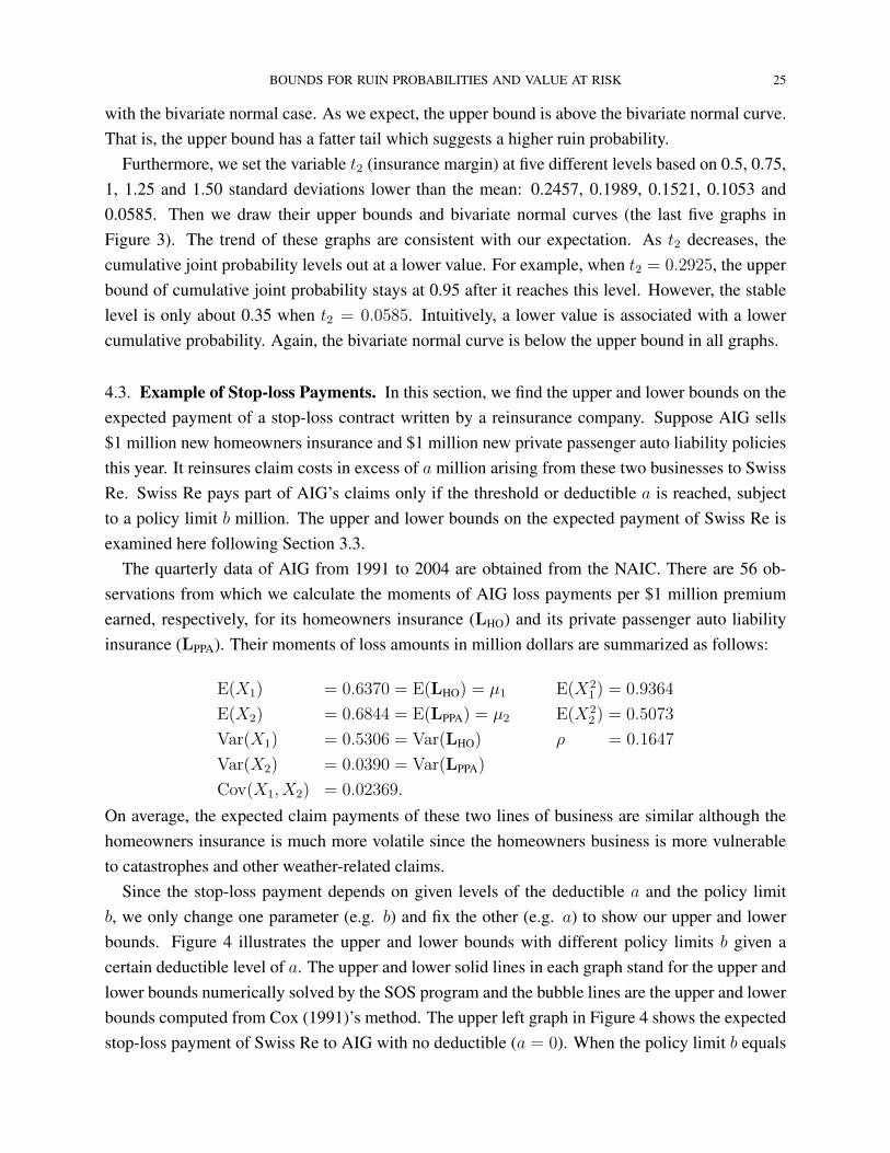
Since the stop-loss payment depends on given levels of the deductible a and the policy limitb, we only change one parameter (e.g. b) and fix the other (e.g. a) to show our upper and lowerbounds. Figure 4 illustrates the upper and lower bounds with different policy limits b given acertain deductible level of a. The upper and lower solid lines in each graph stand for the upper andlower bounds numerically solved by the SOS program and the bubble lines are the upper and lowerbounds computed from Cox (1991)’s method. The upper left graph in Figure 4 shows the expectedstop-loss payment of Swiss Re to AIG with no deductible (a = 0). When the policy limit b equals
26 BOUNDS FOR RUIN PROBABILITIES AND VALUE AT RISK
FIGURE 4. Each plot shows the upper (the top curve in each graph) and lowerbounds (the curve in the bottom) on the expected stop-loss payment. They are afunction of the policy limit b given a level of the deductible a. The solid linesare the upper and lower bounds obtained from the SOS programs. The bubblelines show the upper and lower bound solutions based on the Cox (1991)’s explicitformula. Six graphs fix a at 0, 0.25, 0.5, 0.75, 1 and 1.5 million dollars respectively,with a = 0 on the upper left and running to the right then down. The vertical axisis the expected payment and the horizontal axis is the policy limit b, both in milliondollars.
to $1 million, both methods obtain the same upper and lower bounds, $1 million and $0.7 millionrespectively; when b > 1.5, the lower bound of these two methods matches pretty well while theupper bound of the SOS program levels out at a relatively higher value ($1.4 million) than that ofCox (1991)’s method ($1.3 million). For the cases that the deductible a is fixed at the level 0.5,
BOUNDS FOR RUIN PROBABILITIES AND VALUE AT RISK 27
0.75, 1 or 1.5, the solutions from the SOS and from the explicit formula of Cox (1991)’s methodare almost identical. It suggests that the SOS program works pretty well for this stop-loss paymentproblem. In addition, we should note that SOS program can be flexibly applied to more problems,most of which cannot be explicitly solved.
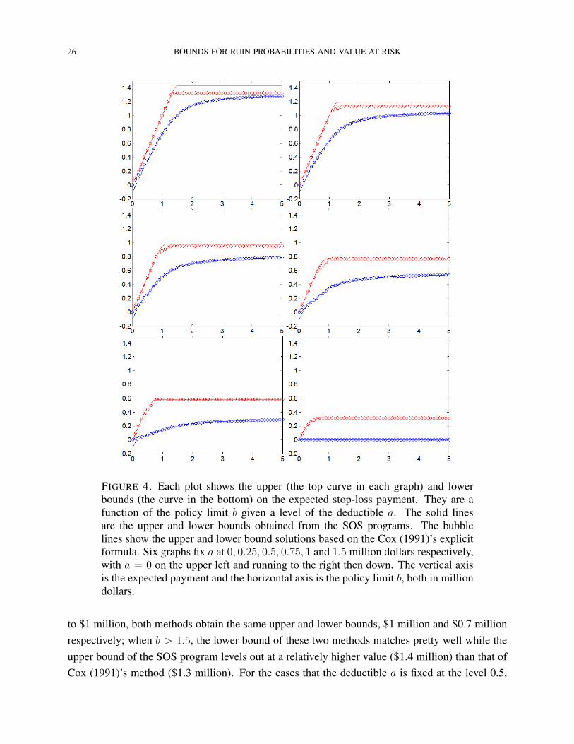
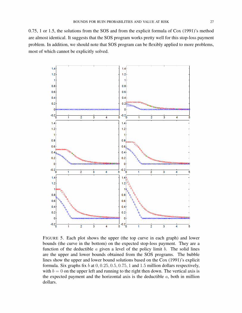
FIGURE 5. Each plot shows the upper (the top curve in each graph) and lowerbounds (the curve in the bottom) on the expected stop-loss payment. They are afunction of the deductible a given a level of the policy limit b. The solid linesare the upper and lower bounds obtained from the SOS programs. The bubblelines show the upper and lower bound solutions based on the Cox (1991)’s explicitformula. Six graphs fix b at 0, 0.25, 0.5, 0.75, 1 and 1.5 million dollars respectively,with b = 0 on the upper left and running to the right then down. The vertical axis isthe expected payment and the horizontal axis is the deductible a, both in milliondollars.
28 BOUNDS FOR RUIN PROBABILITIES AND VALUE AT RISK
To further show the robustness of SOS program solutions, we consider the upper and lowerbounds of a Swiss Re stop-loss policy paying up to a fixed level b while AIG could select differentdeductibles a. Each graph in Figure 5 shows the upper and lower bounds given a certain policylimit b with different deductibles a. As we expect, the bounds on Swiss Re’s expected paymentsincrease as the fixed value b increases (i.e. the stop-loss policy covers more losses). Again, boundscalculated from the SOS program and the Cox (1991)’s method remain qualitatively similar.
5. CONCLUSION
We have extended the application of classical moment problems (or semiparametric methods)to finance, insurance and actuarial science in three ways, all taking into account the correlationbetween different random variables. The first finds bounds on the sum of two variables, given upto second moment information. The second allows us to put “100% confidence intervals” on thejoint probability of two extreme events. The third one computes bounds on the expected paymentof a stop-loss policy, given only the moments of the loss components.
In each case the moment information may be based on historical observations or judgementsfrom scenario analysis. We provide examples to illustrate the potential usefulness of momentmethods in assessing probability of rare events. There are other applications where our approachcould be useful. For example, this approach can be used to estimate the default probability of fixed-income securities, under incomplete knowledge of the enterprise and economic factors driving thecredit risk. In other areas such as inventory and supply chain management, this approach can beapplied to find inventory policies that will be robust to different (unknown) demand distributionsin the future. Even when the distributions of the random variables are assumed to be known,this approach can be implemented to measure sensitivity of the given joint probabilities, VaR andexpected benefits to model misspecification (Lo, 1987; Hobson, Laurence, and Wang, 2005).
REFERENCES
D. Bertsimas and I. Popescu. On the relation between option and stock prices: An optimizationapproach. Operations Research, 50:358–374, 2002.
D. Bertsimas and I. Popescu. Optimal inequalities in probability theory: A convex optimizationapproach. SIAM Journal on Optimization, 15(3):780–804, 2005.
D. Bertsimas and J. Sethuraman. Moment problems and semidefinite optimization. InH. Wolkowitz, R. Saigal, and L. Vandenberghe, editors, Handbook of Semidefinite Program-ming: Theory, algorithms, and applications, pages 469–509. Kluwer, 2000.
D. Bertsimas, K. Natarajan, and C. Teo. Tight bounds on expected order statistics. Probability inthe Engineering and Information Sciences, 20(4):667–686, 2006.
F. Black and M. S. Scholes. The pricing of options and corporate liabilities. Journal of PoliticalEconomy, 81(3):637654, 1973.
BOUNDS FOR RUIN PROBABILITIES AND VALUE AT RISK 29
P. P. Boyle and X. S. Lin. Bounds on contingent claims based on several assets. Journal ofFinancial Economics, 46(3):383–400, 1997.
P. L. Brockett and S. H. Cox. Insurance Calculations using Incomplete Information. ScandinavianActuarial Journal, pages 94–98, 1985.
P. L. Brockett, S. H. Cox, and J. Smith. Bounds on the price of catastrophe insurance options onfutures contracts. In Securitization of Insurance Risks. Society of Actuaries Monograph Series,1996.
K. Bruckner. Quantifying the error of convex order bounds for truncated first moments. Insurance:Mathematics and Economics, 2007. Forthcoming.
S. H. Cox. Bounds on expected values of insurance payments and option prices. Transactions ofthe Society of Actuaries, 43:231–260, 1991.
S. H. Cox, Y. Lin, and S. Wang. Multivariate exponential tilting and pricing implications formortality securitization. Journal of Risk and Insurance, 73(4):719–736, 2006.
D. J. Cummins. Multi-period discounted cash flow ratemaking models in property-liability insur-ance. Journal of Risk and Insurance, 57(1):79–109, 1990.
J. D. Cummins and N. A. Doherty. Can insurers pay for the ‘big one?’ measuring the capacity ofan insurance market to response to catastrophic losses. Working Paper, The Wharton School,University of Pennsylvania, 1997.
P. Diananda. On non-negative forms in real variables some or all of which are non-negative.Mathematical Proceedings of the Cambridge Philosophical Society, 58:17–25, 1962.
S. P. Dokov and D. P. Morton. Second-order lower bounds on the expectation of a convex function.Mathematics of Operations Research, 30(3):662–677, 2005.
W. E. Ferson and A. F. Siegel. The efficient use of conditioning information in portfolios. Journalof Finance, 56(3):967–982, 2001.
W. E. Ferson and A. F. Siegel. Stochastic discount factor bounds with conditioning information.Review of Financial Studies, 16(2):567–595, 2003.
A. R. Gallant, L. P. Hansen, and G. Tauchen. Using conditional moments of asset payoffs to inferthe volatility of intertemporal marginal rates of substitution. Journal of Econometrics, 45(1-2):141–179, 1990.
G. Gallego and I. Moon. The distribution free newsboy problem: review and extensions. Journalof the Operational Research Society, 44:825–834, 1993.
H. U. Gerber, E. S. W. Shiu, and N. Smith. Methods for estimating the optimal dividend barrierand the probability of ruin. Insurance: Mathematics and Economics, 2007. Forthcoming.
B. Grundy. Option prices and the underlying asset’s return distribution. Journal of Finance, 46(3):1045–1069, 1991.
L. P. Hansen and R. Jagannathan. Implications of security market data for models of dynamiceconomies. Journal of Political Economy, 99(2):225–262, 1991.
30 BOUNDS FOR RUIN PROBABILITIES AND VALUE AT RISK
D. Henrion and J. B. Lasserre. GloptiPoly: Global optimization over polynomials with Matlab andSeDuMi. ACM Transactions on Mathematical Software, 29(2):165–194, 2003.
D. Hilbert. Uber die darstellung definiter formen als summe von formenquadraten. MathematischeAnnalen, 32:342–350, 1888.
D. Hobson, P. M. Laurence, and T. H. Wang. Static–arbitrage upper bounds for the prices of basketoptions. Quantitative Finance, 5(4):329–342, 2005.
D. Hong. Asian currency crisis and the impact on regional industrial development.http://notes.tier.org.tw, May 1998.
P.-H. Hsieh. A data-analytic method for forecasting next record catastrophe loss. Journal of Riskand Insurance, 71(2):309–322, 2004.
S. Karlin and W. Studden. Tchebycheff Systems: with Applications in Analysis and Statistics. Pureand Applied Mathematics Vol. XV, A Series of Texts and Monographs. Interscience Publishers,John Wiley and Sons, 1966.
J. H. B. Kemperman. The general moment problem, a geometric approach. Annals of MathematicalStatistics, 38(1):93–122, 1968.
J. H. B. Kemperman. On the sharpness of tchebycheff type inequalities. Indag. Math., 27:554–601,1965.
J. B. Lasserre. Bounds on measures satisfying moment conditions. Annals of Applied Probability,12:1114–1137, 2002.
H. Levy. Upper and lower bounds of put and call option value: stochastic dominance approach.Journal of Finance, 40(4):1197–1217, 1985.
J. Liu, J. Pan, and T. Wang. An equilibrium model of rare-event premia and its implication foroption smirks. Review of Financial Studies, 18(1):131–164, 2005.
A. W. Lo. Semi-parametric upper bounds for option prices and expected payoffs. Journal ofFinancial Economics, 19(2):373–387, 1987.
J. Lofberg. Yalmip : A toolbox for modeling and optimization in MATLAB. In Proceedingsof the CACSD Conference, Taipei, Taiwan, 2004. URL http://control.ee.ethz.ch/∼joloef/yalmip.php.
R. C. Merton. Theory of rational option pricing. Bell Journal of Economics and ManagementScience, 4(1):141–183, 1973.
P. Parrilo. Structured Semidefinite Programs and Semialgebraic Geometry Methods in Robust-ness and Optimization. PhD thesis, Department of Control and Dynamical Systems, CaliforniaInstitute of Technology, Pasadena, CA, 2000.
S. Perrakis and P. J. Ryan. Option pricing bounds in discrete time. Journal of Finance, 39(2):519–525, 1984.
R. D. Phillips, D. J. Cummins, and F. Allen. Financial pricing of insurance in the multiple-lineinsurance company. Journal of Risk and Insurance, 65(4):597–636, 1998.
BOUNDS FOR RUIN PROBABILITIES AND VALUE AT RISK 31
S. Prajna, A. Papachristodoulou, and P. A. Parrilo. Introducing SOSTOOLS:A general purposesum of squares programming solver. In Proceedings of the 41st IEEE Conference on Decisionand Control, pages 741–746. Las Vegas, USA, 2002.
A. Prestel and C. N. Delzell. Positive Polynomials: From Hilbert’s 17th problem to Real Algebra.Springer Monographs in Mathematics. Springer-Verlag, Berlin, 2001.
P. H. Ritchken. On option pricing bounds. Journal of Finance, 40(4):1219–1233, 1985.T. Rockafellar. Convex Analysis. Princeton University Press, Princeton, 1970.B. Roos. On variational bounds in the compound Poisson approximation of the individual risk
model. Insurance: Mathematics and Economics, 2007. Forthcoming.H. Scarf. A min-max solution of an inventory problem. In K. J. Arrow, S. Karlin, and H. Scarf, ed-
itors, Studies in the Mathematical Theory of Inventory and Production, pages 201–209. StanfordUniversity Press, 1958.
A. D. Schepper and B. Heijnen. Distribution-free option pricing. Insurance: Mathematics andEconomics, 2007. Forthcoming.
J. Sturm. Using SeDuMi 1.02, a Matlab toolbox for optimization over symmetric cones. Optimiza-tion Methods and Software, 11–12:545–581, 1999.
M. Todd. Semidefinite optimization. Acta Numerica, 10:515–560, 2001.L. Vandenberghe, S. Boyd, and K. Comanor. Generalized chebyshev bounds via semidefinite
programming. SIAM Review, 49(1):52–64, 2007.J. Yu and Y. Lin. Dynamic capabilities in volatile environments: Evidence from the U.S. prop-
erty and casualty insurance industry. Working Paper, University of Nevada - Las Vegas andUniversity of Nebraska - Lincoln, 2007.
J. Yue, B. Chen, and M. Wang. Expected value of distribution information for the newsvendorproblem. Operations Research, 54(6):1128–1136, 2006.
L. F. Zuluaga. A Conic Programming Approach to Polynomial Optimization Problems: Theoryand Applications. PhD thesis, The Tepper School of Business, Carnegie Mellon University,Pittsburgh, PA, 2004.
L. F. Zuluaga and J. Pena. A conic programming approach to generalized tchebycheff inequalities.Mathematics of Operations Research, 30(2):369–388, 2005.
32 BOUNDS FOR RUIN PROBABILITIES AND VALUE AT RISK
APPENDIX A: PROBABILITY BOUNDS ON Pr(X1 ≥ t1, X2 ≥ t2)
We consider the problem of finding sharp upper and lower bounds on the probability Pr(X1 ≥t1 and X2 ≥ t2) of two non-negative random variables X1, X2, attaining values higher than orequal to t1, t2 ∈ R+ respectively, given up to second order moment information (means, variances,and covariance) onX1, X2, without making any other assumption on the distribution of the randomvariables X1, X2. Finding the sharp upper and lower semiparametric bounds for this problemcan be (respectively) formulated as the following optimization problems, obtained by setting inproblem (2) φ(X1, X2) = I{X1≥t1 and X2≥t2}, and D = R+2 (cf. Section 2):
(38)
p := sup Eπ(I{X1≥t1 and X2≥t2})
such that Eπ(1) = 1,
Eπ(Xi) = µi, i = 1, 2,
Eπ(X2i ) = µ
(2)i , i = 1, 2,
Eπ(X1X2) = µ12,
π a probability distribution in R+2,
and
(39)
p := inf Eπ(I{X1≥t1 and X2≥t2})
such that Eπ(1) = 1,
Eπ(Xi) = µi, i = 1, 2,
Eπ(X2i ) = µ
(2)i , i = 1, 2,
Eπ(X1X2) = µ12,
π a probability distribution in R+2.
Before obtaining the SOS programming formulation of these problems, we discuss its feasibilityin terms of their moments.
Observation 9 (Feasibility). Problems (38) and (39) are feasible if and only if Σ is a positivesemidefinite matrix (i.e., all eigenvalues are greater than or equal to zero) and all elements of Σ
are non-negative, where Σ is the moment matrix:
Σ =
1 µ1 µ2
µ1 µ(2)1 µ12
µ2 µ12 µ(2)2
.Proof. Follows from Diananda’s Theorem (Theorem 2) and convex duality (cf. Rockafellar (1970)).
�
Next we derive SOS programs to numerically compute p, and p by using SOS programmingsolvers.
BOUNDS FOR RUIN PROBABILITIES AND VALUE AT RISK 33
Upper bound. We begin by stating the dual problem of (38):
(40)d = inf y00 + y10µ1 + y01µ2 + y20µ
(2)1 + y02µ
(2)2 + y11µ12
such that p(x1, x2) ≥ I{x1≥t1 and x2≥t2},∀ x1, x2 ≥ 0.
As the following observation states, as long as problem (38) is feasible, we can obtain p bysolving problem (40).
Observation 10 (Strong Duality). Notice that the dual solution y00 = 2, and yij = 0 for (i, j) 6=(0, 0) strictly satisfies (i.e., with >) the constraint in (40) for all x1, x2 ≥ 0. Thus, if problem (38)is feasible, then p = d.
Proof. Follows from convex duality (cf. (Zuluaga and Pena, 2005, Proposition 3.1)). �
To formulate problem (40) as a SOS program, we proceed as follows. First notice that (40) isequivalent to:
(41)
d = inf y00 + y10µ1 + y01µ2 + y20µ(2)1 + y02µ
(2)2 + y11µ12
such that p(x1, x2) ≥ 1,∀ x1 ≥ t1, x2 ≥ t2
p(x1, x2) ≥ 0,∀ x1, x2 ≥ 0.
Applying the substitution x1 → x1 + t1, x2 → x2 + t2 to the first constraint of (41), we havethat (41) is equivalent to:
(42)
d = inf y00 + y10µ1 + y01µ2 + y20µ(2)1 + y02µ
(2)2 + y11µ12
such that p(x1 + t1, x2 + t2)− 1 ≥ 0,∀ x1, x2 ≥ 0
p(x1, x2) ≥ 0, ∀ x1, x2 ≥ 0.
Now let q(x1, x2) = p(x1 + t1, x2 + t2)− 1; that is
q(x1, x2) = (y00 + y10t1 + y01t2 + y20t21 + y02t
22 + y11t1t2 − 1)
+(y10 + 2t1y20 + y11t2)x1
+(y01 + 2t2y02 + y11t1)x2
+y20x21 + y02x
22 + y11x1x2,
so that the first constraint of (42) can be replaced by q(x1, x2) ≥ 0,∀ x1, x2 ≥ 0. To finish, fromTheorem 2, it follows that (42) (with the first constraint written in terms of q(x1, x2)) is equivalentto the following SOS program:
(43)
d = inf y00 + y10µ1 + y01µ2 + y20µ(2)1 + y02µ
(2)2 + y11µ12
such that q(x21, x
22) is a SOS polynomial
p(x21, x
22) is a SOS polynomial.
34 BOUNDS FOR RUIN PROBABILITIES AND VALUE AT RISK
The SOS program (43) can be readily solved with a SOS programming solver. Thus, if prob-lem (38) is feasible (cf. Observation 9), it follows from Observation 10 that we can numericallyobtain the probability semiparametric upper bound p by solving problem (43) with a SOS solver.
Lower bound. We begin by stating the dual problem of (39):
(44)d = sup y00 + y10µ1 + y01µ2 + y20µ
(2)1 + y02µ
(2)2 + y11µ12
such that p(x1, x2) ≤ I{x1≥t1 and x2≥t2},∀ x1, x2 ≥ 0.
As the following observation states, as long as problem (39) is feasible, we can obtain p bysolving problem (44).
Observation 11 (Strong Duality). Notice that the dual solution y00 = −1, and yij = 0 for (i, j) 6=(0, 0) strictly satisfies (i.e., with <) the constraint in (44) for all x1, x2 ≥ 0. Thus, if problem (39)is feasible, then p = d.
Proof. Follows from convex duality (cf. (Zuluaga and Pena, 2005, Proposition 3.1)). �
To formulate problem (44) as a SOS program, we proceed as follows. First notice that (44) isequivalent to:
(45)
d = sup y00 + y10µ1 + y01µ2 + y20µ(2)1 + y02µ
(2)2 + y11µ12
s.t. p(x1, x2) ≤ 1,∀ x1 ≥ t1, x2 ≥ t2
p(x1, x2) ≤ 0,∀ x1 ≥ 0, 0 ≤ x2 ≤ t2,
p(x1, x2) ≤ 0,∀ 0 ≤ x1 ≤ t1, x2 ≥ 0.
Although the first constraint of (45) can be handled as in the upper bound problem (cf. Sec-tion 3.2.1), the last two constraints are difficult to reformulate as SOS constraints. That is, there isno linear transformation from x1 ≥ 0, 0 ≤ x2 ≤ t2 to R+2 or to R2 (that would allow the use ofTheorems 1 and 2). Thus, we change the problem to end up with a SOS program that either solvesor approximates problem (45). Specifically, consider the following problem related to (45):
(46)
d′ = sup y00 + y10µ1 + y01µ2 + y20µ(2)1 + y02µ
(2)2 + y11µ12
such that p(x1, x2) ≤ 1,∀ x1 ≥ t1, x2 ≥ t2
p(x1, x2) ≤ 0,∀ x1 ≥ 0, x2 ≤ t2,
p(x1, x2) ≤ 0,∀ x1 ≤ t1, x2 ≥ 0.
Notice that (46) is less constrained than (45) (the last two constraints of (46) include more valuesof x1 and x2). Thus, d′ is a lower bound on d; that is d′ ≤ d (in fact, intuition suggests that d′ = d).Therefore, d′ and the corresponding upper bound of Section 3.2.1 still give a “100% confidenceinterval” on the value of the cumulative probability of interest.
BOUNDS FOR RUIN PROBABILITIES AND VALUE AT RISK 35
Now, problem (46) is equivalent to (applying variable substitutions similar to the ones used inSection 3.2.1, and multiplying by −1 to get ≥ constraints):
(47)
d′ = sup y00 + y10µ1 + y01µ2 + y20µ(2)1 + y02µ
(2)2 + y11µ12
such that 1− p(x1 + t1, x2 + t2) ≥ 0,∀ x1, x2 ≥ 0
−p(x1, t2 − x2) ≥ 0, ∀ x1, x2 ≥ 0,
−p(t1 − x1, x2) ≥ 0, ∀ x1, x2 ≥ 0.
Similar to the upper bound problem, we now let:
q1(x1, x2) = 1− p(x1 + t1, x2 + t2)
q2(x1, x2) = −p(x1, t2 − x2)
q3(x1, x2) = −p(t1 − x1, x2);
that is,q1(x1, x2) = −(y00 + y10t1 + y01t2 + y20t
21 + y02t
22 + y11t1t2 − 1)
−(y10 + 2t1y20 + y11t2)x1 − (y01 + 2t2y02 + y11t1)x2
−y20x21 − y02x
22 − y11x1x2
q2(x1, x2) = −(y00 + y01t2 + y02t22)
−(y10 + y11t2)x1 − (−y01 − 2y02t2)x2
−y20x21 − y02x
22 + y11x1x2
q3(x1, x2) = −(y00 + y10t1 + y20t21)
−(−y10 − 2y20t1)x1 − (y01 + y11t1)x2
−y20x21 − y02x
22 + y11x1x2.
To finish, from Theorem 2, it follows that (47) (with the first constraint written in terms ofqi(x1, x2), i = 1, . . . , 3) is equivalent to the following SOS program:
(48)
d′ = sup y00 + y10µ1 + y01µ2 + y20µ(2)1 + y02µ
(2)2 + y11µ12
such that q1(x21, x
22) is a SOS polynomial
q2(x21, x
22) is a SOS polynomial
q3(x21, x
22) is a SOS polynomial.
The SOS program (48) can be readily solved with a SOS programming solver. Thus, if prob-lem (39) is feasible (cf. Observation 9), it follows from Observation 11 that we can numericallyapproximate the ruin probability semiparametric lower bound p by solving problem (48) with aSOS solver. Furthermore, notice that by solving (43) and (48) we obtain a “100% confidence in-terval” d′ ≤ Pr(X1 ≥ t1 and X2 ≥ t2) ≤ p on the value of the probability when given only up tothe second order moment information on the non-negative random variables X1, X2.
36 BOUNDS FOR RUIN PROBABILITIES AND VALUE AT RISK
APPENDIX B: OBTAIN BOUNDS ON STOP-LOSS PAYMENTS FROM A TRANSFORMED PROBLEM
Let ψ(Z) = Z − φ(Z) where φ(Z) is the stop-loss payment function defined in problem (25)and ψ(Z) is the transform function (34).
If the moment matrix Σ satisfies the feasibility requirement (cf. Observation 6), we can nu-merically obtain the semiparametric upper bound p(ψ). The upper bound of ψ(Z), p(ψ) =
sup{Eπ[ψ(Z)]} given the same moment information, equals µz minus the lower bound of φ(Z).That is, p(ψ) = µz − p(φ).
Proof. On one side,
(49)
p(ψ) = sup{Eπ[ψ(Z)]}
Eπ[ψ(Z)] = µz − Eπ[φ(Z)]
p(ψ) ≥ µz − Eπ[φ(Z)] ∀π with given moments
p(ψ) ≥ µz − p(φ).
On the other side,
(50)
p(φ) = inf{Eπ[φ(Z)]}
since φ(Z) = Z − ψ(Z)
Eπ[φ(Z)] = µz − Eπ[ψ(Z)]
p(φ) ≤ µz − Eπ[ψ(Z)] ∀π with given moments
p(φ) ≤ µz − p(ψ)
p(ψ) ≤ µz − p(φ).
In order to satisfy both (49) and (50) simultaneously, p(ψ) must equal µz − p(φ). �
The lower bound of ψ(Z), p(ψ) = inf{Eπ[ψ(Z)]} given the same moment information, equalsµz minus the upper bound of φ(Z). That is, p(ψ) = µz − p(φ).
Proof. On one side,
(51)
p(ψ) = inf{Eπ[ψ(Z)]}
Eπ[ψ(Z)] = µz − Eπ[φ(Z)]
p(ψ) ≤ µz − Eπ[φ(Z)] ∀π with given moments
p(ψ) ≤ µz − p(φ).
BOUNDS FOR RUIN PROBABILITIES AND VALUE AT RISK 37
On the other side,
(52)
p(φ) = sup{Eπ[φ(Z)]}
Eπ[φ(Z)] = µz − Eπ[ψ(Z)]
p(φ) ≥ µz − Eπ[ψ(Z)] ∀π with given moments
p(φ) ≥ µz − p(ψ)
p(ψ) ≥ µz − p(φ).
In order to satisfy both (51) and (52) simultaneously, p(ψ) must equal µz − p(φ). �


