Learning from Probabilities: Dependences within Real-Time Systems

Alessandra Melani, Eric Noulard and Luca SantinelliONERA Toulouse, name.surname@onera.fr

Abstract

Realistic real-time systems experience variability and unpre-dictabilities, which can be compensated by potentially very pes-simistic worst-cases. Recent trends apply measurement-basedapproaches in modeling worst-cases with a certain confidence.While observing system evolution it is possible to extract prob-abilistic models to the task execution with a guaranteed prob-abilistic version of worst-case execution time. In this work weexploit such probabilistic models in order to study the effect ofdependences on the task execution time, and we apply the de-veloped probabilistic framework to few relevant cases studies.

1. IntroductionReal-time relies on the Worst-Case Execution Time (WCET)

to model task execution behaviors: a real-time system becomespredictable by always accounting for the worst-case at every taskexecution.

As the input space for the task code is finite and the hardwarebehavior is assumed to be deterministic, it is reasonable to argueabout the exact worst-case execution time. The WCETexactand its estimationC are upper-bounds for any possible executionbehavior of that code [33, 15].

Unfortunately, realistic real-time systems are unpre-dictable [30]. Their environment can be diverse and dy-namic [20], with multiple possible evolutions in time. Bothhardware and software elements may experience some vari-ability or even randomness1, e.g. [multi-]processor cache,branch predictors, DRAM refresh, interruptions that occurwhenever they are most inappropriate [12, 6, 17]. Besides,the interferences between interacting elements in the systemlead to the dependences that emphasize unpredictabilities andvariability. Those are some of the reasons why WCETexact isin general unknown and potentially unknowable. Consequently,the estimation C could be extremely pessimistic.

Probabilities are becoming a consistent way of representingthe time evolution of systems. They are able to model indeter-minacy and unpredictabilities that systems have, since a proba-bilistic representation captures multiple behaviorstogether withtheir frequences. Such a more fine grained system representationreduces the pessimism brought by deterministic models, whereonly the estimation of the worst-case is taken into account. Then,the challenge in real-time is to make predictability out of proba-bilities [5, 7], and build with the probabilities a safe alternativeto the deterministic real-time.

1Randomness intended in the common sense as lack of pattern or predictabil-ity in events

Contributions: In this work, we apply probabilistic modelsand statistical analysis to describe unpredictabilities and dynam-ics that realistic real-time systems have. We target the depen-dences that relate system elements and their concurrent execu-tion. We aim to improve the knowledge of the systems charac-terizing some of their dependences thus reducing the pessimismof their timing models. In doing that, we rely on measurementsand rare events for a probabilistic version of the WCET. Thiswould result into more accurate real-time analyses without theneed of overlaying pessimistic safe bounds and the consequentwaste of resources. To our knowledge, this work is among thefirsts to provide safe and sharp probabilistic WCET bounds forrealistic systems without the need of complicated and artifacthardware elements and models.

Organization of the paper: In Section 2 we introduce theprobabilistic model we intend to apply to characterize tasks ex-ecution times and their worst-cases. Section 3 tackles with thedependences within realistic real-time systems and their effecton the task executions. Section 4 and 5 describe both the exper-iments and their setup we applied to support the theory devel-oped. Section 6 is for the conclusion and the future work.

1.1 Timing Analysis for Real-Time System: the State of theArt

Within the WCET research community a main debate is onthe approaches to the WCET estimation, [33].

On one hand there is the use of static analysis [1, 22, 9, 8],applying models of the code and the underlying hardwarefor WCETstatic estimation. Those analytical approaches canof course be in error, however it is usual to guarantee thatWCETexact < WCETstatic with a possible extra marginadded to the WCETstatic.

On the other hand there are the measurement-based ap-proaches, with a simpler model of the code and the observationsof the task execution time, charging the system effects. TheWCETmeasured is the maximum value observed during mea-surements, but in general WCETmeasured ≤WCETexact, dueto the not assured exhaustive execution condition coverage andthus variability [3]. Even when WCETmeasured is computedusing test generation techniques which ensure feasible path cov-erage, they usually make assumptions which negate variabil-ity, [12, 34].

A more “analytical” approach to measurements makes useof some form of extreme value statistical analysis [13, 14, 21]to construct a predicted WCET value, WCETpredicted. Re-cent works have formally approached Extreme Value Theory(EVT) for the WCET problem [11, 7]. They claim that,with a probabilistic hardware architecture and measurement-based approaches, it is possible to guarantee an accurate

WCETpredicted.Figure 1 gives a further intuition of the differences between

the measurements, the WCETexact (exact) and its safe estima-tion C (safe).

2. The Probabilistic Natural BehaviorDue to variability and unpredictability of today’s real-time

systems, what emerges as their behavior is close to random pro-cesses2. The system indeterminacy is accounted by the manydirections the random process may evolve. In particular, we areinterested in the probabilistic nature of the task execution times,thus their probabilistic representation. With probabilities, it ispossible to enrich the classical notion of worst-case executiontime with further information about the multiple ways tasks canexecute.

Assuming Ci3 a distribution of execution times for a task τias a discrete random variable4, its probabilistic representationthrough probabilistic distribution function (pdf) is fCi

fCi =

(c0i = cmin

i c1i · · · ckii = cmax

i

fCi(cmini ) fCi(c

1i ) · · · fCi(c

maxi ),

)(1)

and∑ki

j=0 fCi(cji ) = 1. All these parameters are given with

the interpretation that task τi generates an infinite number ofsuccessive jobs τi,j , with j = 1, . . . ,∞, and each such jobhas an execution requirement described by Ci, where for eachvalue cki , fCi(c

ki ) is its probability of occurrence within the

execution streamline, P(Ci = cki ). The Cumulative Distribu-tion Function (CDF) description is FCi(c) = P(Ci ≤ c) asFCi(x) =

∑xc=0 fCi(c) for discrete variables, while the inverse

Cumulative Distribution Function (1-CDF) F ′Ci(c) is F ′Ci(c) =1 −

∑xc=0 fCi(c). A representation in terms of 1-CDF outlines

the exceedence thresholds as P{Ci ≥ c}. Figure 2 shows an ex-ample of execution time distribution with its histogram represen-tation for the value frequencies, together with the correspondentCDF and 1-CDF representations.

The task model we consider is τi = (Φi, Ci, Ti, Di), withΦi being the task release time, Ci the distribution of possibleexecution times and associated probabilities, Ti the maximumtask inter-arrival time and Di its relative deadline.

An Execution Time Profile (ETP) Ci of a task τi is a probabil-ity distribution of execution time obtained through exhaustive τiexecution time measurements, the emphirical distribution. Fig-ure 1 shows an example of the execution time profile (measured)with respect to the possible execution time a task can have (pos-sible).

2.1 Dependence between Random Variables

Most of the algebra in probability theory relies on the degreeof dependence between random variables, the so called statisti-cal dependence.

Definition 1 (Independent random variables) Two randomvariables X and Y are independent if they describe two eventssuch that the occurrence of one event does not have any impacton the occurrence of the other event.

2A random process is a sequence of random variables describing a processwhose outcomes do not follow a deterministic pattern, but follow an evolutiondescribed by probability distributions.

3With calligraphic uppercase letters we refer to probabilistic distributions.4Since the execution time of a program can only take discrete values that are

multiples of the processor clock cycle.

execution time

measurements

possible

safe

exact

pro

bab

ilit

y

Figure 1. Execution time profiles, WCET andprobabilistic WCET.

(a) (b)

Figure 2. Histogram, CDF and 1-CDF representa-tion of a task execution times.

An example is the joint probability, which expresses the compo-sition between random variables. For a couple X , Y , the jointprobability defines the probability of events in terms of bothX and Y , P{X = x and Y = y} given by P{Y = y|X =x} · P{X = x} or equivalently P{X = x|Y = y} · P{Y = y}.In terms of CDF it is

FX ,Y(x, y) = FX|Y(x|y) · FY(y) = FY|X (x|y) · FX (x). (2)

Whenever there is independence it is FX ,Y = FX ·FY , whilein case of dependences between X and Y , the joint probabilityremains in its generic form, Equation (2).

Definition 2 (Dependence B) Two random variables X and Yare dependent, X B Y or equivalently Y B X , every time thereis not independence, thus FX|Y(x|y) 6= FX (x).

We will examine later how the dependences come into playwithin our probabilistic framework.

2.2 Probabilistic Worst-Case Execution Time

In a probabilistic scenario, more sound is the notion ofprobabilistic Worst-Case Execution Time distribution, noted aspWCET, that unlike WCETX , it is is a distribution, and not ascalar value. To converge to that notion we need some defini-tions first.

Definition 3 (Greater than or equal to, � [24]) Let X and Ybe two random variables. Y is greater than or equal to X (oralternatively, X is less than or equal to Y) denoted by Y � X(alternatively, Y � X ) if P{Y ≤ v} ≤ P{X ≤ v} for any v(alternatively P{Y ≤ v} ≥ P{X ≤ v} for any v). In termsof the CDF representation, Y � X (Y � X ) if FY ≤ FX(FY ≥ FX ). With the 1-CDF representation, Y � X (Y � X )if F ′Y ≥ F ′X (F ′Y ≤ F ′X ).

With such partial ordering between random variables we can saythat the pWCET distribution is greater than or equal to (meaningworse than but also safer than) the ETPs. A formal definition forthe exact pWCET C∗ is the following.

Definition 4 (probabilistic Worst-Case Execution Time C∗i )The pWCET C∗i of a task τi is defined as the least upper-boundon all the distributions Cji of the execution time of τi, where Cjiis generated for every possible combination j of input data tothe program by running the program an infinite number of times.Thus ∀j, C∗i � C

ji . In terms of CDF FC∗i (x) = minj(FCji

),while the 1-CDF is F ′C∗i (x) = maxj(F

′Cji

).

C∗i is guaranteed to exist knowing all the possible ETPs Cji forthe task τi. Unfortunately, measurement approaches cannot en-sure the coverage of all the execution conditions. Therefore,the pWCET C∗i needs to be estimated, leading to a safe upper-bound Ci. The reasoning is the same as with classical deter-ministic WCET computation, where WCETexact is unknown,which leads to the computation of a possibly safe WCETstaticand WCETpredicted bounds: we aim to compute safe and pos-sibly accurate Ci estimations. With probabilities and measure-ments it is easier to compute distributions Ci from appropriateETP measures, moreover the rare events theory can ensure thesafety of such pWCET estimation Ci. The forthcoming sectionexplains how to get a safe pWCET estimation starting from themeasurements.

2.2.1 From the Measures to the Worst-Cases: the RareEvents

An approach to the pWCET estimation refers to rare events toestimate exceedence probabilities which are smaller than 10−n,where n is a required level of confidence. In this paper we referto the extreme value theory to estimate the probability of occur-rence of extreme values of execution times, known to be rareevents, [13]. More precisely, EVT predicts the distribution func-tion for the maximal (the worst-case) or minimal (the best-case)values of a set of n observations, which are modelled as randomvariables, [11].

The EVT demands certain hypotheses to provide a “good”and “safe” pWCET estimation. The two main hypotheses are in-dependence and identical distribution (i.i.d) of the random vari-ables involved.

The empirical distributions through which we model the ob-servations have to be independent (i.), meaning not sharing anyrelationship or not affecting one another. The presence of anydependence in a series of execution times influences the extremalbehavior of the execution time. Nonetheless, such hypothesis isnot that strict under certain conditions. For processes satisfying aweak mixing condition [29], the degree of long-term dependenceat extreme levels is limited, hence the EVT as the variables wereindependent, is a safe bound.

The identical distribution (i.d.) states that the empirical distri-butions modeling consecutive observations have to repeat iden-tically. This way the EVT would have enough information to ac-curately model the expected rare events from the measurements.Beware that i.d. is a far weaker constraint than the usual de-terministic repeatability. Identical measurement-based distribu-tions may be identical even if every single measure is not repeat-able. This is another key advantage of pWCET over determinis-tic WCET.

3. Real-Time DependencesThe objective of our paper is to study the dependences that

real-time tasks suffer within realistic systems. Cache memories,

scheduling policies, interfering tasks etc. affect the task exe-cution modifying its ETPs and consequently its worst-case, boththe deterministic and the probabilistic ones. With our probabilis-tic framework we intend to quantify such effects studying howthe task execution time distribution varies from the case wherethe interferencing event is not present to the case where it ispresent.

3.1 Formalizing the Dependences

We can envision a real-time system O as a set of events Oj ,O = {O1, O2, . . . On}, where each Oj happens within the sys-tem and participates to both its functional and non-functionalbehavior. Since we are interested in the execution time and whatis affecting it, it is possible to narrow down the set of events tothose which characterize the execution of a task.

The execution of tasks mainly depends on the code that im-plements it. Aside that, but not marginally, there are othersystem elements which influence the task execution and conse-quently its execution time. An event Oj affects Ci if its happen-ing changes the execution time itself and its representing distri-bution Ci. Given a task τi, for those events affecting Ci we couldhave a system representation as

Oi = {Oi1, O

i2, . . .}, (3)

whereOi is the system view with respect to Ci and its effect overCi. For the sake of simplicity, in the rest of the paper we referto O and Oj , respectively for the system representation from τi,and the events affecting Ci.

Among the events affecting task τi execution there are alsothe other tasks τk concurrently executing with τi. Then, for twoevents such as the task execution time Ci and Oj the conditionalprobability describes the effect that Oj has on Ci,

P(Ci|Oj) =P(Ci ∩Oj)

P(Oj)(4)

as the probability of having the execution time Ci once Oj hap-pens. In this paper we will not consider all the possible eventsaffecting the task execution time; instead, we begin the analysis

with some of them. With Ci|Ojdef= Ci,Oj

and P(Ci|Oj)def=

P(Ci,Oj), the conditional probability joints events putting to-

gether the task execution time and the effect of Oj on it. Ingeneral Ci,Oj 6= Ci, due to the dependence relationship betweenCi and Oj .

Lemma 1 (Independence of the CDF) Assuming two depen-dent execution time random variables Ci and Ck, the randomvariable Ci|Ck is independent from Ck and FCk = FCk|Ci|Ck .

Proof: With Ci and Ck dependent, it is FCi,Ck = FCi|CkFCk =FCk|CiFCi . Considering the execution time distribution Ci|Ckwith FCi|Ck its CDF representation, it is FCi|Ck,Ck = FCi|Ck|Ck ·FCk = FCk|Ci|Ck · FCi|Ck .FCi|Ck|Ck = FCi|Ck and FCi|Ck,Ck = FCi|Ck · FCk stating the

independence between Ci|Ck and Ck. Furthermore,

FCi|Ck|CkFCk = FCk|Ci|CkFCi|Ck = FCi|CkFCk , (5)

so that FCk = FCk|Ci|Ck ; then the lemma follows.

With the improved description Ci,Ojof the task execution it

is also possible to conclude about the independence of the exe-cution time conditional distribution with respect to any system

event Oj . For example, with Ci B Ck, thanks to Lemma 1, Ci,Ck

is independent from Ck, being P(Ci,Ck|Ck) = P(Ci,Ck

). In fact,considering an event Oj , once its effects are included inside theconditional distribution of execution times of τi, Ci,Oj

, they willno longer affect it, i.e. the main task will run independently fromthat event. Obviously, Lemma 1 can be generalized to considerany kind of distribution, not only execution time distributions.

It is worth noting that a very wide variety of events can fit inthe set O: this mostly depends on the abstraction level we maywant to consider,Oj = Cj . For instance, the presence of anothertask τj running together with the main one could be representedat a finer level of detail as the distribution of execution times itgenerates. The main consequence of this reasoning is that anyevent could have an associated probability distribution function,even trivial such as a binary random variable. What matters toensure the applicability of Lemma 1 is the existence of that dis-tribution, regardless of its shape.

3.2 Dependence Composability

With Equation (3) and Equation (4), it is possible to decom-pose the dependence problem into sub-problems following theidea of set partitioning. Thus, the execution time of a task τi,Ci,O, is composed by all the effects from the events Oj whichare related to the execution time.

In such a probabilistic scenario we can define the isolationas a system configuration where the task τi is not influenced bythe rest of the system. While executing in isolation, the taskexperiences ETPs Ci with no effects from other tasks or sys-tem elements. Then, it is possible to define the notion of not-isolation, as a system configuration where the task receives in-terference from the elements composing the system configura-tion, O = {O1, O2, . . .}. In the next section we will see how toinstantiate the isolation and not-isolation for realistic real-timesystems.

3.3 Toward the Characterization of the Dependences

The study of dependences within a probabilistic real-timeframework are mostly associated with copulas, [2]. In this paperwe re-formulate the basics of copulas for the characterization ofrandom variables dependences and enhance the analysis to real-istic and complex real-time systems.

In a first approximation, we can think about a measure ofthe dependence as a distance between the two random vari-ables. Then, a difference ∆i between two execution time dis-tributions Ci and C′i, in terms of 1-CDFs, could be represented as∆i = maxx|F ′Ci(x)−F ′C′i(x)|. A meaningful difference among1-CDFs would be the one that considers the shift of a distribu-tion,

∆i,Oj = min{∆|∀c F ′Ci(c−∆) ≥ F ′Ci,Oj(c)}. (6)

∆i,Oj characterizes the effect thatOj has on τi and its executiontime; hence it is a measure of the dependence between Oj andCi. Then ∆i,Oj

can be seen as the cost required in order tocreate independence between Ci andOj . With Equation (6), it ispossible to upper-bound the dependence between Ci and any ofthe events Oj composing O with a distribution C′i,Oj

such that

F ′upC′i,Oj

(c)def= F ′Ci(c−∆i,Oj ); (7)

We have now a distribution ables to bound the independent caseCi|Oj .

Theorem 1 (Independence Bound) Given a task τi with exe-cution time distribution Ci in isolation. In case τi executes to-gether with another event Oj the resulting execution time dis-tribution is Ci,Oj

. The distribution C′i,Ojsuch that F ′upC′i,Oj

(c) =

F ′Ci(c−∆i,Oj ) with ∆i,Oj = min{∆|F ′Ci(c−∆) ≥ F ′Ci,Oj(c)}

represents an upper-bound to the independence case between Ci

and Oj , Ci|Oj .

Proof: We distinguish three cases. In the case ∆i,Oj= 0, which

states the independence between Ci and Oj , ∀c F ′Ci|Oj(c) =

F ′Ci(c), and no influence comes from the event Oj to Ci. Then∀c F ′upC′i,Oj

(c) = F ′Ci,Oj(c) = F ′Ci(c), upper-bounding such inde-

pendence case.With ∆i,Oj

> 0, it is ∀c FCi|Oj(c) > FCi(c) and

F ′Ci(c) ≤ F′Ci|Oj

(c) ≤ F ′upC′i,Oj

(c); (8)

then, F ′upC′i,Oj

upper-bounds the independence case Ci|Oj , Ci,Oj.

Finally, with ∆i,Oj < 0, it is F ′Ci,Oj(c) < F ′Ci(c)∀c, and

F ′Ci|Oj(c) ≤ F ′upC′i,Oj

(c) ≤ F ′Ci(c) (9)

by the definition of bounding, Equation (6). Although FCi is asafe bound, it could be very pessimistic; then C′i,Oj

as F ′upC′i,Oj

rep-

resents a more accurate upper-bound to the independenceCi|Oj .

With such bound F ′upC′i,Oj

, it is possible to safely carry on the prob-

abilistic real-time analyses with the independence hypothesis,see [24] as an example that requires task independence assump-tion.

4. Experimental setupIn this section we expose the characteristics (hardware and

software) of the experiments we set up in order to begin investi-gating the dependences within real-time systems.

4.1 Tracing Instrumentation

The main goal of our experimental setup is the appropriatemeasurement of execution time profiles for various real-timetask sets. Since we want to address any kind of execution target,we cannot rely on simulation: neither a cycle accurate one, norany hardware-specific assisted observation, because those maynot be available. Therefore, we have to go for instrumented real-time execution, often called tracing.

The performance monitoring tool we have chosen, LTTng(Linux Trace Toolkit new generation) [16], adheres to theparadigm of static tracing, which is usually performed by addinglogging statements to the code and compiling them with the pro-gram. This kind of instrumentation can be suitable to supportreal-time critical activities, since it achieves low overhead at theonly payback of a small increase in the code size. It allowsstatic collection of timestamped traces, for both kernel and user-space events, together with a new powerful feature, namely thepossibility of appending to trace events performance monitor-ing counters [32]. This possibility allows to monitor with greatprecision the behavior of the cache, which is among the eventsaffecting tasks executions that we intend to investigate.

In our measurements we collect as less data as possible, in or-der to minimize perturbation, and we use hardware performancecounters when available, e.g. for counting cache misses.

4.2 Architecture

All the experiments have been run on a machine having twoIntel R©Xeon R©E5620 2.4 GHz sockets, each one with four coresand three levels of cache. The first two levels (L1 and L2) are“per core”, while the last level (L3) is “per socket”, hence sharedamong each group of four cores. The L1 cache is partitioned into32 KB data cache and 32 KB instruction cache, while L2 and L3(respectively 256 KB and 12 MB) are unified.

With the kernel boot parameter isolcpus5 we specify the set ofcores that we may want to isolate from the general SMP balanc-ing and scheduling algorithms. Exploiting this option, the firstfour cores have been reserved to our experiments, while the gen-eral scheduling was bounded to the remaining ones. Likewise,all the interrupts have been redirected on the second CPU, exceptthose preventing the correct behavior of the system, for exampletiming, performance monitoring and non-maskable ones. Thissetup constitutes the embodiment of the definition of isolationwe gave in section 3.2.

4.3 Execution Environment: SCHEDMCORE

SCHEDMCORE6 is an open source integrated developmentframework for critical embedded systems [10], which providestwo main tools: the SCHEDMCORE CONVERTER, a valida-tion tool which, after transforming a task model description intoa formally analyzable model in C or UPPAAL, can performschedulability analysis, and the SCHEDMCORE RUNNER, anexecution tool which envisions precise real-time execution on amulti-core architecture, using various real-time scheduling poli-cies. The tools take as input a file describing the task model(either as a textual description or a PRELUDE library [28]). TheSCHEDMCORE CONVERTER was used to ensure that the usedtask set was theoretically schedulable. The SCHEDMCORE run-time, used by the SCHEDMCORE RUNNER, is implemented asa user-space library, which means that the Linux kernel does notneed to be patched and that it can be maintained without follow-ing the evolution of the underlying OS. This user-space approachhas been used in the past [23] in order to avoid the burden of go-ing inside the OS kernel; even more recently the same approachin [26] has been proven efficient as well.

Besides the system isolation setup we described previously,SCHEDMCORE tools and runtime ensure usual real-time exe-cution: memory lock, switching to real-time scheduling policy,bounding each thread (runtime or user) to its own private core,and so on.

In order to ease and automatize the experiments, SCHEDM-CORE framework may load during startup a scheduler plugin(FP, EDF, LLREF, etc.), which implements the scheduling pol-icy at user level, as well as any kind of C function [25] to be usedfor the implementation of the real-time task. The configurationis specified in the task file description [25] for one part and therest of it from the command line [27], i.e. the taskset descriptionis defined in the taskfile, whereas real-time parameters like schedpolicy, binding, time base etc. are specified from the commandline.

5 ExperimentsThree are the benchmarks that we study, all of them taken

from the Malardalen Benchmark suite [19]. The first one, “jfd-5see <kernelsrc>/Documentation/kernel-parameters.txt6https://forge.onera.fr/projects/schedmcore

ctint”, is a simple single-path benchmark with a small data foot-print, but a consistent code size. The second one, “cnt”, ismore data consistent, but still single-path benchmark. Finally,we tackle with the complexity of a multi-path case by exploitingthe “nsichneu” benchmark.

These three benchmarks are the beginning of a more complexanalysis we intend to develop. We consider them significativesince they explore varios aspectcs such as the data and instruc-tion cache as well as the multi-path problem.

Within a realistic real-time system, by isolation (ISO) we in-tend the execution of the task under analysis with the fewestpossible effects from the system, i.e. reduced number of ac-tive interrupts, smallest set of system calls, single core affinityand no other functional tasks running on the same core. Thetested scheduling policies range from Non-Preemptive (NP) toFixed Priority (FP) and Earliest Deadline First (EDF). The ex-periments we carried on consider the isolation case as baselinefor comparing execution time and cache misses values.

We further investigate the cache effects on task executiontime with two distinct cache interferences in case of preemption:those coming from preemptive tasks performing simple CPUburning (“burn”), and those from preemptive tasks performingmore consistent cache activities (“cache”).

In this stage of the work, we deal with an observed task τiand an interfering task τj , either preempting or not. Accordingto the different configurations tested, both τi and τj are asked tochange in order to better exploit the system events under investi-gation. The measured quantities for each job of τi are the a) re-sponse time in µsec, b) execution time in µsec, c) L1-Instructioncache load misses, d) L1-Data cache load misses, e) L3 cacheload misses and the f) number of context switches.

5.1 EVT Applicability

We make use of the Gumbel distribution to describe the tailbehavior of execution times. On the measurements we have car-ried out few tests to verify the EVT applicability. The first isthe exponential tail test [18], to check that the execution timeobservations effectively fit a Gumbel distribution [11]. All ourempirical distributions ETP pass that test.

Then, we have tested the i.d. hypothesis with the two-sampleKolmogorov-Smirnov test [31], in which two samples of 5000execution time observations are compared. The test verifies thattwo samples out of the ETPs are identically distributed.

Finally, the independence hypothesis has been tested with theruns test [4], looking for randomness between consecutive ob-servations. For most of the observations such test fails due tothe small variability of the execution time we have. The onlyexception is the multi-path benchmark, where multiple paths areexercised at each execution. This increases the randomness de-gree of consecutive observations. Although not independent, ourmeasurements follow a linear dependence or stationarity, thatwe verified with linear correlation indexes. The linear depen-dence guarantees the EVT to be a good tail projection for theETPs, [29].

Table 5.1 has the results from the Kolmogorov-Smirnov test,the run test and the correlation (Pearson’s correlation coeffi-cient) test to samples of 10,000 execution time observations, ap-plied to some of the observations considered. Represented isthe probability of obtaining a test statistic at least as extreme asthe one that was actually observed assuming the null hypothe-

jfdctint ISO cnt ISO nsichneu ISO nsichneu FPi.d. 0.95 0.89 0.87 0.51i. < 2.2e− 16 < 2.2e− 16 < 2.2e− 16 0.45

linear 0.3 −0.8 0.15 0.005

Table 1. p-values for the i.i.d. and linear corre-lation tests. jfdctint in isolation, cnt in isolation,nsichneu in isolation and nsichneu with preemp-tions are reported.

sis true, in our case the hypotheses of being i.d., i., and lineardependence. The p-value less than the predetermined signifi-cance level, often 0.05, indicates that the observed result wouldbe highly unlikely under the null hypothesis. Thus, we can ac-cept both the i.d. and the linear dependence hypotheses but notthe i. hypothesis.

5.2 Simple Benchmark: jfdctint

The jfdctint benchmark performs a JPEG integer implemen-tation of a forward discrete-cosine transform on a reduced datastructure of 8x8 pixel block.

We begin considering the effects produced by the interferenceof a preempting task τj , in both “burn” and “cache” configura-tions. Figure 3 shows that the latter exhibits a larger executiontime profile, especially in the tail-end region. In the same fig-ure, we also represent the upper-bound to the task ETPs, whichtakes into account the preemption costs relative to both “burn”and “cache” configurations. Such upper-bound F ′upC′i,Oj

(upper-

bound in the figure), defined in Equation (7), where Oj is thepreemption event. The preemption effect to the jfdctint τi can bebounded by ∆i,Oj = 80µsec out of around 1.2sec as maximumexecution time, Equation (6). With an ETP as the one defined byF ′upC′i,Oj

, we can assume τi to be independent from the preemption

effect.

1100 1150 1200 1250 1300

1e-05

1e-03

1e-01

Execution Time

Probability

ISOlp-burnlp-cacheupper-bound

Figure 3. jfdctint: isolation, non-preemptive andpreemptive case comparison.

By exploring the scheduling policy and its effects on the taskexecution time we notice how the higher scheduling overheadfrom EDF with respect to the FP scheduler, determines a sub-stantial increase in the execution time profile, as can be seen inFigure 4. An upper-bound to the scheduler effects is quantifiedwith F ′upC′i,Oj

and ∆i,Oj= 108µsec.

We have also taken into account the number of preemptionsτi experiences. In particular, the overhead related to the contextswitch and the indirect effects on cache may determine a furtherincrease in the execution time. For a simple benchmark as theone we are considering, only a small variation is perceived while

1100 1150 1200 1250 1300 1350

1e-05

1e-03

1e-01

Execution Time

Probability

ISOFPEDFupper-bound

Figure 4. jfdctint: scheduling policy comparison.

increasing the number of preemptions, Figure 5. This is due tothe almost negligible context switch overhead with respect tothe task computation time jfdctint has. We can notice that mul-tiple preemptions do not change considerably the task largestobserved values; nonetheless, their main effect remains the in-crease of the average task execution time, between 6000µsecsand 6040µsecs.

5960 5980 6000 6020 6040

1e-05

1e-03

1e-01

Execution Time

Probability

1xP2xP3xP

Figure 5. jfdctint: number of preemptions com-parison. The execution times are much largerthan the previous jfdctint tests due to few modi-fications required in order to exploit multiple pre-emptions from other tasks.

5.3 Heavy Data-structured Benchmark: cnt

The cnt benchmark counts the number of non-negative valuesinside a square matrix, which is randomly initialized. We applyit to analyze in detail the contribution of the cache effects onthe task execution time. In particular, leaving constant the datastructure of the observed task τi, we play with the data size of theinterfering task τj implemented with the cnt function, in orderto draw conclusions on the effect that cache misses have on theexecution time.

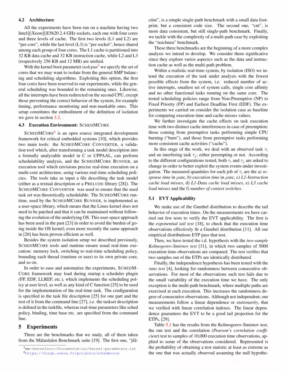
The set of ETPs of Figure 6 captures the great variability thatwe achieve when the data structure of the preempting task isprogressively augmented. We observe a substantial increase inthe execution time for average values, because the heavier thedata structure of τj is the more cache trashing is created duringthe preemptions. Nonetheless, this trend does not translate intoa proportional growth of the largest execution time values. In-deed the isolation configuration has larger execution time thanthe “burn” case as well as the “cache” case with 1000x1000 datastructure. This is due to other phenomena which characterizemodern processor architectures such as prefetch and branch pre-diction. Although not yet able to properly model those effects,our measurement-based approach can observe them and the ef-

fects they provoke. In the future, we will make an effort to com-plete our probabilistic modeling framework and include them in.An F ′upC′i,Oj

built as in Equation (7) (the upper-bound in the figure)

with ∆i,Oj= 124µsec upper-bounds all these effects.

13500 13600 13700 13800 13900

1e-05

1e-03

1e-01

Execution Time

Probability

ISOburncache 750x750cache 1000x1000upper-bound

Figure 6. cnt: execution time comparison.

In terms of extreme value theory this pWCET estimation Ci,Figure 7 shows that we can achieve great accuracy with our ob-served values due to the accuracy of our ETP measurements.Then, with the Ci and the EVT applied, we can safely performprobabilistic scheduling analysis [24], assuming independencebetween tasks for the configurations studied with cnt, as statedby Theorem 1.

13500 13600 13700 13800 13900 14000

1e-05

1e-03

1e-01

Execution Time

Probability

upper-bound EVTupper-bound obs

Figure 7. cnt: extreme value theory of the execu-tion time.

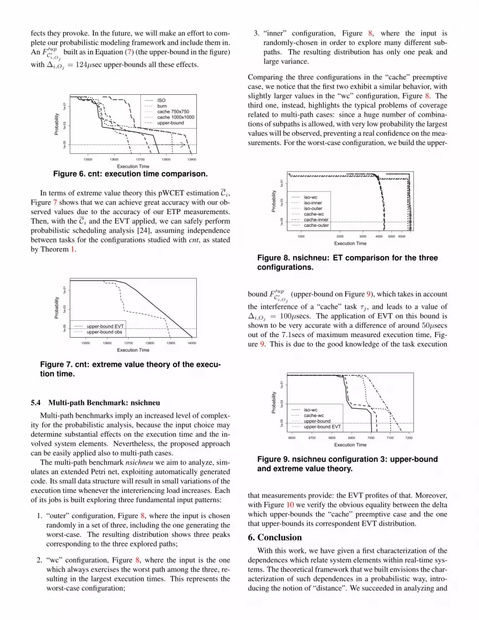
5.4 Multi-path Benchmark: nsichneu

Multi-path benchmarks imply an increased level of complex-ity for the probabilistic analysis, because the input choice maydetermine substantial effects on the execution time and the in-volved system elements. Nevertheless, the proposed approachcan be easily applied also to multi-path cases.

The multi-path benchmark nsichneu we aim to analyze, sim-ulates an extended Petri net, exploiting automatically generatedcode. Its small data structure will result in small variations of theexecution time whenever the intereriencing load increases. Eachof its jobs is built exploring three fundamental input patterns:

1. “outer” configuration, Figure 8, where the input is chosenrandomly in a set of three, including the one generating theworst-case. The resulting distribution shows three peakscorresponding to the three explored paths;

2. “wc” configuration, Figure 8, where the input is the onewhich always exercises the worst path among the three, re-sulting in the largest execution times. This represents theworst-case configuration;

3. “inner” configuration, Figure 8, where the input israndomly-chosen in order to explore many different sub-paths. The resulting distribution has only one peak andlarge variance.

Comparing the three configurations in the “cache” preemptivecase, we notice that the first two exhibit a similar behavior, withslightly larger values in the “wc” configuration, Figure 8. Thethird one, instead, highlights the typical problems of coveragerelated to multi-path cases: since a huge number of combina-tions of subpaths is allowed, with very low probability the largestvalues will be observed, preventing a real confidence on the mea-surements. For the worst-case configuration, we build the upper-

1000 2000 3000 4000 5000 6000

1e-05

1e-03

1e-01

Execution Time

Probability

iso-wciso-inneriso-outercache-wccache-innercache-outer

Figure 8. nsichneu: ET comparison for the threeconfigurations.

bound F ′upC′i,Oj

(upper-bound on Figure 9), which takes in account

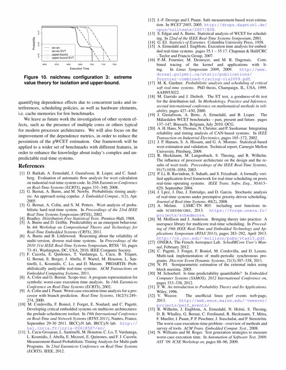
the interference of a “cache” task τj , and leads to a value of∆i,Oj

= 100µsecs. The application of EVT on this bound isshown to be very accurate with a difference of around 50µsecsout of the 7.1secs of maximum measured execution time, Fig-ure 9. This is due to the good knowledge of the task execution

6600 6700 6800 6900 7000 7100 7200

1e-05

1e-03

1e-01

Execution Time

Probability

iso-wccache-wcupper-boundupper-bound EVT

Figure 9. nsichneu configuration 3: upper-boundand extreme value theory.

that measurements provide: the EVT profites of that. Moreover,with Figure 10 we verify the obvious equality between the deltawhich upper-bounds the “cache” preemptive case and the onethat upper-bounds its correspondent EVT distribution.

6. ConclusionWith this work, we have given a first characterization of the

dependences which relate system elements within real-time sys-tems. The theoretical framework that we built envisions the char-acterization of such dependences in a probabilistic way, intro-ducing the notion of “distance”. We succeeded in analyzing and

6600 6700 6800 6900 7000 7100 7200

1e-05

1e-03

1e-01

Execution Time

Probability

iso-wciso-wc EVTupper-boundupper-bound EVT

Figure 10. nsichneu configuration 3: extremevalue theory for isolation and upper-bound.

quantifying dependence effects due to concurrent tasks and in-terferences, scheduling policies, as well as hardware elements,i.e. cache memories for few benchmarks.

We leave as future work the investigation of other system ef-fects, such as the presence of multiple cores or others typicalfor modern processor architectures. We will also focus on theimprovement of the dependence metrics, in order to reduce thepessimism of the pWCET estimation. Our framework will beapplied to a wider set of benchmarks with different features, inorder to enhance the knowledge about today’s complex and un-predictable real-time systems.

References[1] D. Barkah, A. Ermedahl, J. Gustafsson, B. Lisper, and C. Sand-

berg. Evaluation of automatic flow analysis for wcet calculationon industrial real-time system code. In 20th Euromicro Conferenceon Real-Time Systems (ECRTS), pages 331–340, 2008.

[2] G. Bernat, A. Burns, and M. Newby. Probabilistic timing analy-sis: An approach using copulas. J. Embedded Comput., 1(2), Apr.2005.

[3] G. Bernat, A. Colin, and S. M. Petters. Wcet analysis of proba-bilistic hard real-time system. In Proceedings of the 23rd IEEEReal-Time Systems Symposium (RTSS), 2002.

[4] Bradley. Distribution-Free Statistical Tests. Prentice-Hall, 1968.[5] A. Burns and D. Griffin. Predictability as an emergent behaviour.

In 4th Workshop on Compositional Theory and Technology forReal-Time Embedded Systems (CRTS), 2011.

[6] A. Burns and B. Littlewood. Reasoning about the reliability ofmulti-version, diverse real-time systems. In Proceedings of the2010 31st IEEE Real-Time Systems Symposium, RTSS ’10, pages73–81, Washington, DC, USA, 2010. IEEE Computer Society.

[7] F. Cazorla, E. Quinones, T. Vardanega, L. Cucu, B. Triquet,G. Bernat, E. Berger, J. Abella, F. Wartel, M. Houston, L. San-tinelli, L. Kosmidis, C. Lo, and D. Maxim. PROARTIS: Prob-abilistically analysable real-time systems. ACM Transactions onEmbedded Computing Systems, 2011.

[8] A. Colin and G. Bernat. Scope-tree: A program representation forsymbolic worst-case execution time analysis. In 14th EuromicroConference on Real-Time Systems (ECRTS), 2002.

[9] A. Colin and I. Puaut. Worst case execution time analysis for a pro-cessor with branch prediction. Real-Time Systems, 18(2/3):249–274, 2000.

[10] M. Cordovilla, F. Boniol, J. Forget, E. Noulard, and C. Pagetti.Developing critical embedded systems on multicore architectures:the prelude-schedmcore toolset. In 19th International Conferenceon Real-Time and Network Systems (RTNS 2011), Nantes, France,September 29-30 2011. IRCCyN lab, IRCCyN lab. http://hal.inria.fr/inria-00618587/en/.

[11] L. Cucu-Grosjean, L. Santinelli, M. Houston, C. Lo, T. Vardanega,L. Kosmidis, J. Abella, E. Mezzeti, E. Quinones, and F. J. Cazorla.Measurement-Based Probabilistic Timing Analysis for Multi-pathPrograms. In 23nd Euromicro Conference on Real-Time Systems(ECRTS). IEEE, 2012.

[12] J.-F. Deverge and I. Puaut. Safe measurement-based wcet estima-tion. In WCET’2005, 2005. http://drops.dagstuhl.de/opus/volltexte/2007/808.

[13] S. Edgar and A. Burns. Statistical analysis of WCET for schedul-ing. In 22nd of the IEEE Real-Time Systems Symposium, 2001.

[14] G. EJ. Statistics of Extremes. Columbia University Press, 1958.[15] A. Ermedahl and J. Engblom. Execution time analysis for embed-

ded real-time systems. pages 35.1 – 35.17. Chapman & Hall/CRC- Taylor and Francis Group, 2007.

[16] P.-M. Fournier, M. Desnoyer, and M. R. Dagenais. Com-bined tracing of the kernel and applications with lt-tng. In Linux Symposium 2009, 2009. http://www.dorsal.polymtl.ca/static/publications/fournier-combined-tracing-ols2009.pdf.

[17] M. K. Gardner. Probabilistic analysis and scheduling of criticalsoft real-time systems. PhD thesis, Champaign, IL, USA, 1999.AAI9953022.

[18] M. Garrido and J. Diebolt. The ET test, a goodness-of-fit testfor the distribution tail. In Methodology, Practice and Inference,second international conference on mathematical methods in reli-ability, pages 427–430, 2000.

[19] J. Gustafsson, A. Betts, A. Ermedahl, and B. Lisper. TheMalardalen WCET benchmarks – past, present and future. pages137–147, Brussels, Belgium, July 2010. OCG.

[20] A. H. Hans, N. Thomas, N. Christer, and P. Sasikumar. Integratingreliability and timing analysis of CAN-based systems. In IEEETransaction on Industrial Electronics, pages 165–172, 2002.

[21] J. P. Hansen, S. A. Hissam, and G. A. Moreno. Statistical-basedwcet estimation and validation. Technical report, Carnegie MellonUniversity, Pittsburg, 2009.

[22] R. Heckmann, M. Langenbach, S. Thesing, and R. Wilhelm.The influence of processor architecture on the design and the re-sults of wcet tools. Proceedings of the IEEE Real-Time Systems,91(7):1038–1054, 2003.

[23] P. Li, B. Ravindran, S. Suhaib, and S. Feizabadi. A formally veri-fied application-level framework for real-time scheduling on posixreal-time operating systems. IEEE Trans. Softw. Eng., 30:613–629, September 2004.

[24] J. Lpez, J. Daz, J. Entrialgo, and D. Garcia. Stochastic analysisof real-time systems under preemptive priority-driven scheduling.Journal of Real-time Systems, 40(2), 2008.

[25] A. Melani. LSMC-TN #03: including user functions in-side SCHEDMCORE, 2013. https://forge.onera.fr/projects/schedmcore.

[26] M. Mollison and J. Anderson. Bringing theory into practice: Auserspace library for multicore real-time scheduling. In Proceed-ing of 19th IEEE Real-Time and Embedded Technology and Ap-plications Symposium (RTAS’2013), pages 283–292, April 2013.http://cs.unc.edu/˜mollison/pubs/rtas13.pdf.

[27] ONERA, The French Aerospace Lab. SchedMCore User’s Man-ual, February 2012.

[28] C. Pagetti, J. Forget, F. Boniol, M. Cordovilla, and D. Lesens.Multi-task implementation of multi-periodic synchronous pro-grams. Discrete Event Dynamic Systems, 21(3):307–338, 2011.

[29] N. PJ. Semiparametric estimation of the extremal index usingblock maxima. 2005.

[30] M. Schoeberl. Is time predictability quantifiable? In EmbeddedComputer Systems (SAMOS), 2012 International Conference on,pages 333–338, 2012.

[31] F. W. An introduction to Probability Theory and Its Applications.Wiley, 1996.

[32] V. Weaver. The unofficial linux perf events web-page,2013. http://web.eece.maine.edu/˜vweaver/projects/perf_events/.

[33] R. Wilhelm, J. Engblom, A. Ermedahl, N. Holsti, S. Thesing,D. B. Whalley, G. Bernat, C. Ferdinand, R. Heckmann, T. Mitra,F. Mueller, I. Puaut, P. P. Puschner, J. Staschulat, and P. Stenstrom.The worst-case execution-time problem - overview of methods andsurvey of tools. ACM Trans. Embedded Comput. Syst., 2008.

[34] N. Williams and M. Roger. Test generation strategies to measureworst-case execution time. In Automation of Software Test, 2009.AST ’09. ICSE Workshop on, pages 88–96, 2009.