Population size estimation based upon ratios of recapture probabilities

arX

iv:1

107.

5423

v1 [

stat

.AP]

27

Jul 2

011

The Annals of Applied Statistics

2011, Vol. 5, No. 2B, 1512–1533DOI: 10.1214/10-AOAS436c© Institute of Mathematical Statistics, 2011

POPULATION SIZE ESTIMATION BASED UPON RATIOS OFRECAPTURE PROBABILITIES

By Irene Rocchetti1, John Bunge2 and Dankmar Bohning

Sapienza University of Rome, Cornell University and University of Reading

Estimating the size of an elusive target population is of promi-nent interest in many areas in the life and social sciences. Our aimis to provide an efficient and workable method to estimate the un-known population size, given the frequency distribution of counts ofrepeated identifications of units of the population of interest. Thiscounting variable is necessarily zero-truncated, since units that havenever been identified are not in the sample. We consider several ap-plications: clinical medicine, where interest is in estimating patientswith adenomatous polyps which have been overlooked by the diag-nostic procedure; drug user studies, where interest is in estimatingthe number of hidden drug users which are not identified; veteri-nary surveillance of scrapie in the UK, where interest is in estimatingthe hidden amount of scrapie; and entomology and microbial ecology,where interest is in estimating the number of unobserved species of or-ganisms. In all these examples, simple models such as the homogenousPoisson are not appropriate since they do not account for present andlatent heterogeneity. The Poisson–Gamma (negative binomial) modelprovides a flexible alternative and often leads to well-fitting models.It has a long history and was recently used in the development ofthe Chao–Bunge estimator. Here we use a different property of thePoisson–Gamma model: if we consider ratios of neighboring Poisson–Gamma probabilities, then these are linearly related to the countsof repeated identifications. Also, ratios have the useful property thatthey are identical for truncated and untruncated distributions. In thispaper we propose a weighted logarithmic regression model to estimatethe zero frequency counts, assuming a Gamma–Poisson distribution

Received November 2009; revised October 2010.1Supported by Sapienza University of Rome, grant “Mixed Effect Models for Hetero-

geneous Data Modeling.”2This research was conducted using the resources of the Cornell University Center for

Advanced Computing, which receives funding from Cornell University, New York State,the National Science Foundation and other leading public agencies, foundations and cor-porations. Supported by NSF Grant DEB-08-16638.

Key words and phrases. Chao–Bunge estimator, Katz distribution, species problem,negative binomial distribution, weighted linear regression, zero-truncation.

This is an electronic reprint of the original article published by theInstitute of Mathematical Statistics in The Annals of Applied Statistics,2011, Vol. 5, No. 2B, 1512–1533. This reprint differs from the original inpagination and typographic detail.

1

http://arxiv.org/abs/1107.5423v1

http://www.imstat.org/aoas/

http://dx.doi.org/10.1214/10-AOAS436

http://www.imstat.org

http://www.imstat.org

http://www.imstat.org/aoas/

http://dx.doi.org/10.1214/10-AOAS436

2 I. ROCCHETTI, J. BUNGE AND D. BOHNING

for the counts. A detailed explanation about the chosen weights anda goodness of fit index are presented, along with extensions to otherdistributions. To evaluate the proposed estimator, we applied it to thebenchmark examples mentioned above, and we compared the resultswith those obtained through the Chao–Bunge and other estimators.The major benefits of the proposed estimator are that it is definedunder mild conditions, whereas the Chao–Bunge estimator fails tobe well defined in several of the examples presented; in cases wherethe Chao–Bunge estimator is defined, its behavior is comparable tothe proposed estimator in terms of Bias and MSE as a simulationstudy shows. Furthermore, the proposed estimator is relatively in-sensitive to inclusion or exclusion of large outlying frequencies, whilesensitivity to outliers is characteristic of most other methods. Theimplications and limitations of such methods are discussed.

1. Introduction. The size N of an elusive population must often bedetermined. Elusive populations occur, for example, in public health andmedicine, agriculture and veterinary science, software engineering, illegal be-havior research, in the ecological sciences and in many other fields [Bishop,Fienberg and Holland (1995), Bunge and Fitzpatrick (1993), Chao et al.(2001), Hay and Smit (2003), Pledger (2000, 2005), Roberts and Brewer(2006), Wilson and Collins (1992)]. A prominent problem in public health isthe completeness of a disease registry [Van Hest et al. (2008)], while an inter-esting application of capture–recapture techniques in the veterinary sciencesis the estimation of hidden scrapie in Great Britain [Bohning and Del RioVilas (2008)]. In software engineering [Wohlin, Runeson, and Brantestam(1995)] we are interested in finding the number of errors hidden in softwarecomponents. In criminology the number of people with illegal behavior isof high interest [Van der Heijden, Cruyff, and Houwelingen (2003)], and inecology we wish to estimate the number of rare species of organisms [Chao etal. (2001)]. All of these situations fall under the following setting. We assumethat there are N units in the population, which is closed (no birth, death ormigration), and that there is an endogenous mechanism such as a register,a diagnostic device, a set of reviewers, or a trapping system, which identifiesn distinct units from the population. A given unit may be identified exactlyonce, or it may be observed twice, three times, or more. We denote the num-ber of units observed i times by fi, so that n= f1+f2+f3+ · · ·; the numberof unobserved or missing units is f0, so N = f0 +n. The objective is to findan estimate (or rather a prediction) f0 for f0, and hence an estimate N of N .

To illustrate, we first introduce several examples from different domains;these are analyzed in the following sections:

1. Methamphetamine use in Thailand. Surveillance data on drug abuse areavailable for 61 health treatment centers in the Bangkok metropolitanregion from the Office of the Narcotics Control Board (ONCB). Using

POPULATION SIZE ESTIMATION BASED UPON RATIOS 3

Table 1

Methamphetamine data—frequency distribution of treatment episodes per drug user

f1 f2 f3 f4 f5 f6 f7 f8 f9 f10 n

3114 163 23 20 9 3 3 3 4 3 3345

this data, it was possible to reconstruct the counts of treatment episodesfor each patient in the last quarter of 2001. Table 1 presents the number ofmethamphetamine users for each count of treatment episodes [Bohninget al. (2004)]; the maximum observed frequency was 10. Here we areinterested in estimating the number of hidden methamphetamine users.

2. Screening for colorectal polyps. In 1990, the Arizona Cancer Center ini-tiated a multicenter trial to determine whether wheat bran fiber canprevent the recurrence of colorectal adenomatous polyps [Alberts et al.(2000), Hsu (2007)]. Subjects with previous history of colorectal ade-nomatous polyps were recruited and randomly assigned to one of twotreatment groups, low fiber and high fiber. The researchers noted thatadenomatous polyp data are often subject to unobservable measurementerror due to misclassification at colonoscopy. It can be assumed thatpatients with a positive polyp count were diagnosed correctly, whereasit is unclear how many persons with zero-count of polyps were false-negatively diagnosed. Thus, we approach the data as if zero-counts werenot observed, and we try to estimate the undercount from the nonzerofrequencies. Table 2 shows the polyp frequency data for the two differenttreatment groups; the (overall) maximum frequency is 77. The number ofsubjects with an observed number of adenomas equal to 0 is 285 for theLow Fiber treatment and 381 for High Fiber treatment respectively; weregard this as an undercount and seek to estimate the true unobservedfrequencies f0.

Table 2

Polyps data—frequency distribution of recurrent adenomatous polyps per patient, bytreatment group

(f0) f1 f2 f3 f4 f5 f6 f7 f8 f9 f10 f11 · · ·

Low (285) 145 66 39 17 8 8 7 3 1 0 3 · · ·

High (381) 144 61 55 37 17 5 4 6 5 1 1 · · ·

f22 · · · f28 · · · f31 · · · f44 · · · f57 · · · f70 · · · f77 n

Low 1 · · · 1 · · · 0 · · · 0 · · · 0 · · · 0 · · · 0 299High 0 · · · 0 · · · 1 · · · 1 · · · 1 · · · 1 · · · 1 341


Table 3

Scrapie data—frequency distribution of the scrapie countwithin each holding for Great Britain in 2005

f1 f2 f3 f4 f5 f6 f7 f8 n

84 15 7 5 2 1 2 2 118

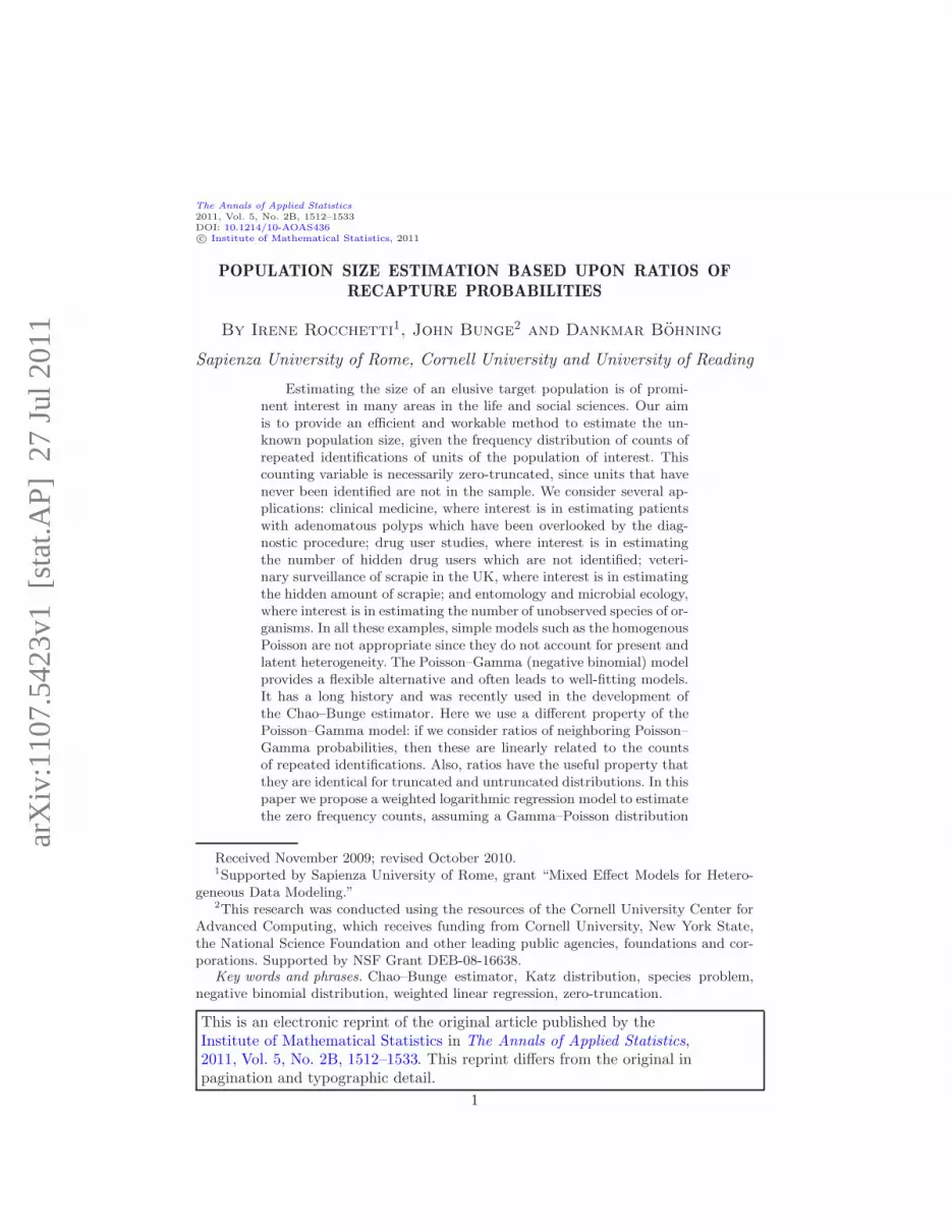
3. Scrapie in Great Britain. Sheep are kept in holdings in Great Britainand the occurrence of scrapie in the population of holdings is monitoredby the Compulsory Scrapie Flocks Scheme [Bohning and Del Rio Vilas(2008)]. This was established in 2004 and summarizes three surveillancesources. Table 3 presents the frequency distribution of the scrapie count

within each holding for the year 2005. Here interest is estimating f0,the frequency of holdings with unobserved or unreported scrapie. Themaximum frequency in the data is 8.

4. Malayan butterfly data. This data set derives from a large collection ofMalayan butterflies collected by A. S. Corbet in 1942 [Fisher, Corbetand Williams (1943)]. There were 9031 individual butterflies classified ton = 620 species. Out of these 620 different species, 118 were observedexactly once, 74 twice, 44 three times and so forth. This “abundance”data is shown in Table 4. Fisher, Corbet and Williams (1943) reportedexact counts only up to f24, stating that there were a total of 119 specieswith sample abundances (counts) greater than 24. Here the interest is inestimating the total number of species N .

5. Microbial diversity in the Gotland Deep. The data on microbial diversityshown in Table 5 stem from a recent work by Stock et al. (2009). Mi-crobial ecologists are interested in estimating the number of species Nin particular environments. Unlike butterflies, microbial species member-ship is not clear from visual inspection, so individuals are defined to bemembers of the same species (or more general taxonomic group) if theirDNA sequences (derived from a certain gene) are identical up to somegiven percentage, 95% in this case. Here the study concerned protistandiversity in the Gotland Deep, a basin in the central Baltic Sea. Thesample was collected in May 2005. The maximum observed frequencywas 53.

Table 4

Butterfly data—frequency distribution of butterfly species collected in Malaya

f1 f2 f3 f4 f5 f6 f7 f8 f9 f10 f11 f12

118 74 44 24 29 22 20 19 20 15 12 14

f13 f14 f15 f16 f17 f18 f19 f20 f21 f22 f23 f24 f>24 n

6 12 6 9 9 6 10 10 11 5 3 3 119 620


Table 5

Protistan diversity in the Gotland Deep—frequency counts of observed species

f1 f2 f3 f4 f6 f8 f9 f10 f11

48 9 6 2 2 2 1 2 1

f12 f13 f16 f17 f18 f20 f29 f42 f53 n

1 1 2 1 1 1 1 1 1 84

The classical approach to estimation of N is to assume that each popula-tion unit enters the sample independently with probability p (dealing withheterogeneous capture probabilities by modeling and averaging). Given p,the unbiased Horvitz–Thompson estimator of N is n/p, and the maximumlikelihood estimator is its integer part ⌊n/p⌋. One then estimates p using anyof several methods, and the final estimate of N is n/p or ⌊n/p⌋ [Lindsay andRoeder (1987), Bohning et al. (2005), Bohning and van der Heijden (2009),Wilson and Collins (1992), Bunge and Barger (2008), Chao (1987, 1989),Zelterman (1988)].

Here we take a new approach: we consider ratios of successive frequency

counts, namely,

r(x) :=(x+1)fx+1

fx.

Often r(x) appears as a roughly linear function of x, which leads us to applylinear regression to the scatterplot of (x, r(x)); we then project the regression

function downward to the left, to zero, which yields f0 and hence N . Figure 1shows the ratio plot of (x, r(x)) for the methamphetamine data; there isclear evidence for a linear trend. Projecting the line to the left, we obtainf0 = 57,788 and, hence, N = 61,133.

Figure 2 shows the ratio plot for the butterfly data; again there is a clearlinear trend and here we also observe increasing variance in the points as xincreases, which we will deal with via weighted least squares. In this case wefind f0 = 126 and N = 746.

This simple and powerful method applies exactly when the frequencycounts emanate from the Katz family of distributions, namely, the bino-mial, Poisson and gamma-mixed Poisson or negative binomial, and it ap-plies approximately to extensions of the Katz family and to general Poissonmixtures. It can be implemented using any statistical software package thatperforms weighted least squares regression, and it is superior to existingmethods for the negative binomial model (including maximum likelihood)in several ways. In addition, it substantially mitigates the effect of truncatinglarge counts (recaptures or replicates), which is an issue with almost everyexisting method, parametric or nonparametric. In Section 2 we discuss the


Fig. 1. Scatterplot with regression line of (x+1)f(x+1)/fx vs. x for the Bangkok metham-phetamine drug user data.

method and its scope of applicability; in Section 3 we describe weightingschemes; in Section 4 we look at goodness of fit of the linear model; andin Section 5 we compare our method with existing techniques, analyze thefive data sets, and discuss the implications of our findings. The Appendixcovers aspects of the approximation used for reaching the linear model aswell as a comparative simulation study, a discussion of standard error ap-proximations, and an assessment of the effect of deleting large “outlying”frequencies.

Fig. 2. Scatterplot with regression line of (x+1)f(x+1)/fx vs. x for the butterfly data.


2. Linear regression and the Katz distributions. Let p0, p1, p2, . . . denotea probability distribution on the nonnegative integers. The condition

(x+1)px+1

px= γ + δx, x= 0,1,2, . . . ,(2.1)

where γ and δ are real constants, characterizes the Katz family of dis-

tributions [Johnson, Kemp and Kotz (2005)]. To yield a valid probabilitydistribution, it is necessary that γ > 0 and δ < 1. If δ < 0, px is the binomialdistribution; if δ = 0, px is the Poisson; and if δ ∈ (0,1), px is the negativebinomial. These distributions arise naturally as models for population sizeestimation.

• Suppose that a given population unit may be observed on each of k “trap-ping occasions.” Assume further that the trapping or capture probability,say, r, is the same on each occasion and that captures are independentacross occasions, and also that the capture probability is the same (ho-mogeneous) for all units, and that units are captured independently ofeach other. If mi denotes the number of captures of the ith unit, thenm1, . . . ,mN are i.i.d. binomial (k, r) random variables. This simple modelis rarely realistic, but it can provide a lower bound for the populationsize, since the homogeneity assumption leads to downwardly biased esti-mation in the presence of heterogeneity. This is formally proved in Bohningand Schon (2005) for maximum likelihood estimation. In this case the fre-quency count data f1, f2, . . . summarizes the nonzero values ofm1, . . . ,mN .

• Now suppose that population unit i appears a random number of timesmi in the sample, but now m1, . . . ,mN are i.i.d. Poisson random variableswith (homogeneous) mean λ. This model arises naturally in species abun-

dance sampling where each species contributes some number of represen-tatives to the sample; it also appears as an approximation to the binomialmodel with λ≈ kr, for large k and small r. Again the homogeneity makesthis model mainly useful for lower-bound benchmarking.

• Assume now that the foregoing Poisson model holds, but with the mod-ification that the mean number of appearances of unit i is λi, and thatλ1, . . . , λN are i.i.d. gamma-distributed random variables. Then the distri-bution of mi is (unconditionally) gamma-mixed Poisson, that is, negativebinomial. This is not the simplest possible model with heterogeneous cap-ture rates, but it may be the oldest, appearing in Fisher, Corbet andWilliams (1943), the source of our butterfly data. (Note that it includesthe geometric, since the exponential is a special case of the gamma.) Thenegative binomial distribution is widely applicable as a model for the fre-quency counts, when the data is not too highly skewed (left or right);however, it is surprisingly difficult to fit by, for example, maximum likeli-hood, or by other existing procedures such as the Chao–Bunge estimator


(see discussion below). We show below that, when implemented by ourweighted least squares regression procedure, the negative binomial modelbecomes practical and useful for estimating N in a variety of situations.

We make two further comments on distribution theory. First, it may bereadily shown using the Cauchy–Schwarz inequality that the ratio on theleft-hand side of (2.1) is nondecreasing for any mixed-Poisson distribution.This means that the linear relation, and hence our weighted linear regressionprocedure below, can be regarded as a first-order linear approximation forany Poisson mixture (not just gamma), thus justifying a degree of robustnessof our method across a wide range of heterogeneity models. Second, thereare extended versions of relation (2.1) which give rise to distributional ex-tensions of the Katz family that need not be mixed-Poisson [Johnson, Kempand Kotz (2005)]. Such extensions may be parameterized and we conjecturethat our method below will be robust to small perturbations along theseparameters.

Condition (2.1) suggests linear regression of the left-hand side upon theright, in some form. Observe that the natural estimate of px would bepx(N) := fx/N , if N were known. But

(x+1)px+1(N)

px(N)=

(x+1)fx+1/N

fx/N=

(x+1)fx+1

fx= r(x),

so we can fit a linear regression of r(x) on x without knowing N . We can

then obtain an estimate of f0 by setting x = 0 so that r(0) = 1f1/f0 = γ,

and, hence, f0 = f1/γ. In practice, however, we prefer to fit the response ona logarithmic scale, which is approximately linear near the origin and avoidsnegative fitted values. Thus, our basic equation becomes

log

((x+1)px+1

px

)= γ + δx,

and we fit the model

log

((x+ 1)fx+1

fx

)= γ + δx+ εx.(2.2)

We consider this in terms of linear regression in the next section. The esti-mate of f0 is then f0 = f1e

−γ .In particular, consider the gamma-mixed Poisson or negative binomial

model for the count data. Let the negative binomial be parameterized as

p(x) =Γ(x+ k)

Γ(x+1)Γ(k)pk(1− p)x,

where k > 0 and p ∈ (0,1). Similar to other areas such as Poisson regression,we need to apply a suitable transformation to avoid negative values for the


ratios which would lead to negative estimates for f0. The log-transformationis appropriate, although others are also possible. Transforming both sides,we obtain

log{(x+1)p(x+1)/p(x)}= log(x+ k) + log(1− p),

but now the right-hand side is nonlinear in k. However, taking the first-orderTaylor expansion of log(k+ x) around k, we achieve

log(k+ x)≈ log(k) +1

kx,

so that we have log(x+k)+ log(1−p)≈ log(1−p)+ log(k)+x/k. Note thatthis approximation is exact for x= 0 (the point where we predict) and goodfor x= 1 (corresponding to the informative “singleton” frequency count). Inthe Appendix we discuss this approximation further, as well as alternatives.With reference to model (2.2), we have γ = log(1− p)+ log(k) and δ = 1/k.We focus on this model in the discussion below.

Note also that due to the simple structure of the estimator f0 = f1 exp(−γ),we can use conditioning [Bohning (2008)] in combination with the δ-method

to give an approximate expression for the variance of f0 as

Var(f0)≈ exp(−γ)2f1[Var(γ)f1 +1],

where Var(γ) is the variance of the intercept estimator in the regression

model. An approximation to the variance of N = f0 + n is then [using the

same technique and estimating Var(n) =N(1− p0)p0 by nf0/N ]

Var(N)≈ nf0

N+ exp(−γ)2f1[Var(γ)f1 +1].(2.3)

Standard errors are obtained by plugging in estimates for Var(γ) and tak-ing the (overall) square root. These expressions may be imprecise for smallsample sizes (<100) and in such cases the bootstrap might be preferable.We provide a simulation study on this aspect in the Appendix.

3. Heteroscedasticity and weighted least squares. Model (2.2) does notsatisfy the classical linear regression assumptions. In the first place, theresponse is discrete (although log-transformed), so we might consider a gen-eralized linear model such as Poisson or even negative binomial regression.However, this is inadvisable since an appropriate formulation as a gener-alized linear model leads to an autoregressive equation involving log fx asan additional offset term in the linear predictor. These kinds of models ex-perience difficulties in terms of the definition of the likelihood as well as incarrying out inference. Actually, residuals derived from model (2.2) typicallyshow reasonable conformity with normal probability plots when the linear


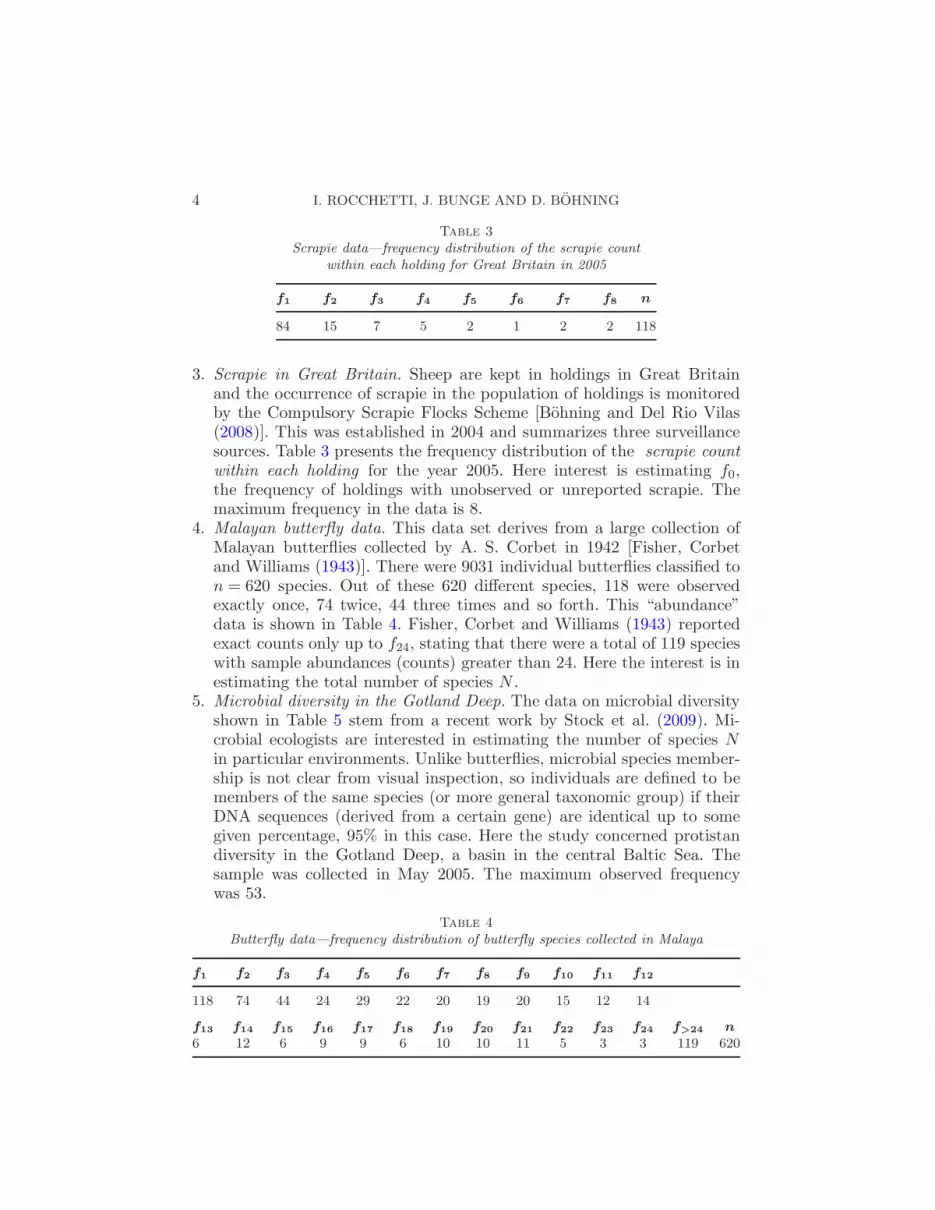
model fits well (see Section 4 regarding goodness of fit). The issues of de-pendence and heteroscedasticity are more important, and we address theseby using weighted least squares. We take

(γδ

)= (XT

WX)−1X

TWY,

where

Y =

log( 2f2f1

)

log( 3f3f2

)

...

log(mfmfm−1

)

, X=

1 11 2...

...1 m− 1

,

and m is the maximum frequency used in the estimator (see Section 4 belowregarding truncation of large frequencies). To reduce MSE, we wish to takeW ≈ (cov(Y))−1. To find cov(Y), assume that the distribution of the cellcounts f1, . . . , fm is multinomial with cell probabilities π = (π1, . . . , πm)T .Then it is well known that f = (f1, . . . , fm)T has covariance matrix Σ =n[Λ(π) − ππT ], where Λ(π) is a diagonal matrix with elements π on thediagonal, and n= f1 + · · ·+ fm. Writing

Σ= n[Λ(π)− ππT ] = Λ(nπ)−1

nnπnπT ,

we see that Σ can be estimated as

Σ = Λ(f)−1

nf f

T .

An application of the multivariate delta-method then shows that an estimateof cov(Y) is

∇f (Y(f))Σ(∇Tf (Y(f)))

(3.1)

=

1f1

+ 1f2

−1f2

0 . . . 0 . . . 0−1f2

1f2

+ 1f3

−1f3

0 . . . 0

0. . .

.... . .

0 . . . 0 −1fi

1fi+ 1

fi+1

−1fi+1

0 . . . 0

.... . .

0 0 −1fm−1

1fm−1

+ 1fm

.

Note that this requires that only nonzero frequencies be used in the esti-mate.


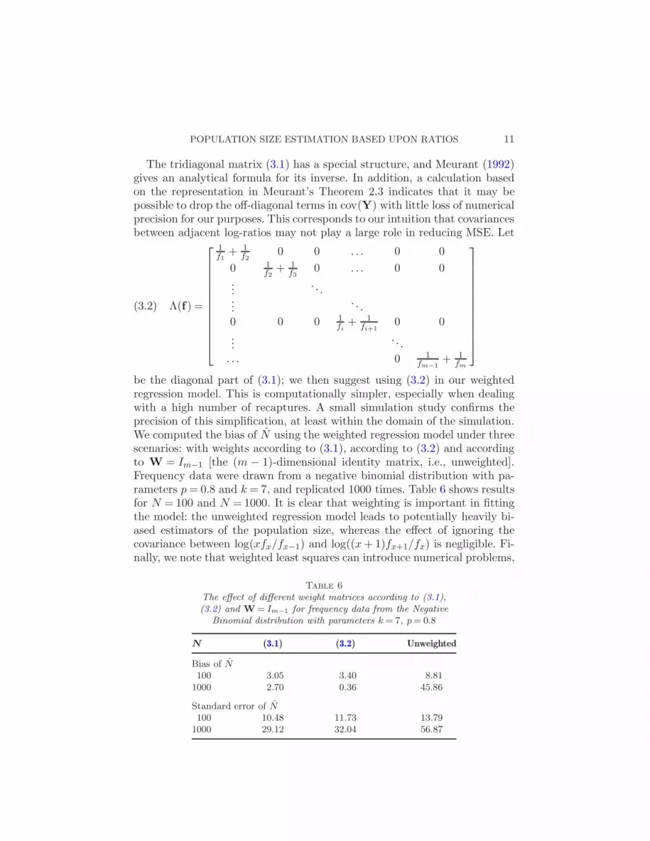
The tridiagonal matrix (3.1) has a special structure, and Meurant (1992)gives an analytical formula for its inverse. In addition, a calculation basedon the representation in Meurant’s Theorem 2.3 indicates that it may bepossible to drop the off-diagonal terms in cov(Y) with little loss of numericalprecision for our purposes. This corresponds to our intuition that covariancesbetween adjacent log-ratios may not play a large role in reducing MSE. Let

Λ(f) =

1f1

+ 1f2

0 0 . . . 0 0

0 1f2

+ 1f3

0 . . . 0 0...

. . ....

. . .

0 0 0 1fi+ 1

fi+10 0

.... . .

. . . 0 1fm−1

+ 1fm

(3.2)

be the diagonal part of (3.1); we then suggest using (3.2) in our weightedregression model. This is computationally simpler, especially when dealingwith a high number of recaptures. A small simulation study confirms theprecision of this simplification, at least within the domain of the simulation.We computed the bias of N using the weighted regression model under threescenarios: with weights according to (3.1), according to (3.2) and accordingto W = Im−1 [the (m − 1)-dimensional identity matrix, i.e., unweighted].Frequency data were drawn from a negative binomial distribution with pa-rameters p= 0.8 and k = 7, and replicated 1000 times. Table 6 shows resultsfor N = 100 and N = 1000. It is clear that weighting is important in fittingthe model: the unweighted regression model leads to potentially heavily bi-ased estimators of the population size, whereas the effect of ignoring thecovariance between log(xfx/fx−1) and log((x+1)fx+1/fx) is negligible. Fi-nally, we note that weighted least squares can introduce numerical problems,

Table 6

The effect of different weight matrices according to (3.1),(3.2) and W= Im−1 for frequency data from the Negative

Binomial distribution with parameters k = 7, p= 0.8

N (3.1) (3.2) Unweighted

Bias of N100 3.05 3.40 8.81

1000 2.70 0.36 45.86

Standard error of N100 10.48 11.73 13.79

1000 29.12 32.04 56.87


especially in sparse-data situations [Bjorck (1996), Chapters 4 and 6]; how-ever, our design matrix has only rank 2 and our maximum frequency m istypically not too large, so we have not yet encountered such problems here.This is a topic for future research in this context.

4. Model assessment and goodness of fit. The ratio plot shown in Fig-ure 1 is our main graphical tool for looking at goodness of fit of the linearregression model, and having fit the model, the standard diagnostic plotsof residuals are also available. We also require a quantitative assessment ofoverall fit: R2 could be used based on the response log(x+1)fx+1/fx, but inthis setting it seems more appropriate to work on the original frequency ofcounts scale. In addition, we are looking for a measure which allows analysisof residuals. We therefore compare the observed frequencies with the esti-mated frequencies from the model, using the χ2-statistic as a goodness-of-fitmeasure [Agresti (2002)]. The estimated frequencies based on the regressionmodel are

yx = log(x+1)fx+1

fx= γ + δx,

x= 1,2, . . . ,m, or, equivalently,

(x+ 1)fx+1

fx= exp(yx),

where m is the “truncation point” or maximum frequency used in the anal-ysis (we return to this issue below). In general, the estimated ratios of fre-

quencies fx+1/fx need not uniquely determine fx+1 and fx, but in this case

they do since f0 = f1/ exp(γ) = f1/(f1/f0). This also shows that f1 = f1,

since f0 = f1/ exp(γ) = f1/ exp(y0), and, hence, f1 = f0 exp(y0) = f1. Now,

with f1 given the equation 2f2/f1 = 2f2/f1 determines f2 uniquely, leading

to the recursive relation fx+1 = fx exp(yx)/(x+ 1), x = 1,2, . . . ,m− 1. Wethen define our χ2 statistic as

χ2 =

m∑

x=1

(fx − fx)2

fx

and simulations support that this has a χ2 distribution with m− 2 degreesof freedom if the regression model yx = γ + δx is correct. Note that wehave m unconstrained frequencies, since n=

∑mx=1 fx is random, and we lose

2 degrees of freedom due to estimating the intercept and slope parameters.Note also that the estimate of the intercept parameter fixes f1 = f1, so thatthe degrees of freedom are indeed only reduced by 2. This approach has thebenefit of gaining one degree of freedom when compared to a goodness-of-fit


measure based solely on the regression model which works with the m− 1values yx, x= 1, . . . ,m− 1.

This argument is conditional upon fixing the value of m, and, indeed, allknown procedures for population size estimation truncate large “outlier” fre-quencies in some way. To illustrate, we return to the classical maximum like-lihood (ML) approach. Bunge and Barger (2008) describe a procedure whichfits the desired distribution (here, the negative binomial) to the (nonzero)frequency count data by ML; the estimate of N is then based upon theestimated parameter values of the distribution. Typically, parametric distri-butions can only be made to fit the data up to some truncation point m,beyond which the fit, as assessed by the classical Pearson χ2 test, falls offconsiderably; consequently, only frequencies up to m are used to obtain theestimate of N , and the number of units with frequencies greater than mis added to the estimate ex post facto. Bunge and Barger (2008) proposea goodness-of-fit criterion for selecting m, while the coverage-based non-parametric methods of Chao and co-authors fix m heuristically at 10 [seeChao and Bunge (2002)]. Our weighted linear regression approach also hasthe potential for loss of fit as m increases, depending on the realized struc-ture of the data, and again we can fix m prior to the analysis, and collapseall frequencies greater than this threshold to one value. Sensitivity of thevarious methods to the choice of m is a complex topic [Bunge and Barger(2008) compute all estimates at all possible values of m]; however, our dataanalyses below show that the weighted linear regression model is consider-ably less sensitive to m than its chief competitors in the negative binomialcase, namely, ML and the Chao–Bunge estimator.

Finally, we note that in the ML approach, if the negative binomial fitis less than ideal (although perhaps still acceptable), numerical maximumlikelihood algorithms often do not converge, or converge to the edges of theparameter space, which in turn distorts the apparent fit. The regression-based method described here offers a more robust approach to parameterestimation, and appears not to be prone to the numerical problems whicharise for maximum likelihood estimation under the negative binomial model.In fact, the negative binomial parameter estimates (p, k) derived from theregression model and could be used as starting values for a numerical searchfor the ML estimates. This is a topic for further research.

5. Alternative estimators, data analyses and discussion.

5.1. Alternative estimators. We first consider certain other options forthe negative binomial model.

• Maximum likelihood. This approach is well studied and has a long history[see Bunge and Barger (2008)], but as noted above, good numerical solu-tions for the model parameters (p, k) seem to be remarkably difficult to


obtain, even using reasonably sophisticated search algorithms with high-precision settings. In our experience we get good numerical convergenceonly when the frequency data is smooth and fits the negative binomialwell, or the right-hand tail is fairly severely truncated. The latter issuecauses the additional computational burden of investigating a diversity oftruncation points, each involving numerical optimization. Nonetheless, wecan obtain ML results for the negative binomial in some cases. The MLestimator NML is consistent for N given that the model is correct.

• Chao–Bunge. Let τ denote the probability of observing a unit at leasttwice, that is, τ = 1− p0 − p1. Chao and Bunge (2002) developed a non-parametric estimator τ for τ , and on this basis proposed the estimator

NCB :=m∑

j=2

fjτ

for N . They showed that NCB is consistent for N under the negative bino-mial model. However, in applied data analysis τ may be very small or evennegative, leading to very large or negative values of NCB. This is one rea-son that Chao and Bunge set m= 10 (as noted above). In fact, NCB fails

roughly as often as NML, although not necessarily in the same situations.• Chao. Chao (1987, 1989) proposed the nonparametric statistic

NCh = n+f21

2f2,

which is valid as a (nonparametric) lower bound for N ; we compute ithere as a benchmark. Note that m≡ 2.

We are currently investigating the asymptotic behavior of our estimator Nin detail. Here we can make the following observations. First, assume thatthe upper frequency cutoff m is selected as m=max{j :fi > 0, i= 1, . . . , j},so that m is a random variable. For the unweighted case, that is, W= Im−1

in Section 3 above, it may be readily shown that N/N → 1 in probabilityas N →∞, when either Y = [(i+1)fi+1/fi] and (i+1)pi+1/pi = γ+ δi (theKatz condition), or Y = [log((i+1)fi+1/fi)] and log((i+1)pi+1/pi) = γ+δi.If W = (cov(Y))−1 or a diagonal matrix with positive variances as entries(similar to those discussed in Section 3), then we conjecture that analogousresults can be obtained (here W must be a function of m). The convergencequestion is more complex for a weight matrix W that is estimated andperhaps approximated further (as in Section 3), although we believe thata Slutsky-type argument will again yield the desired consistency result. Inany case, we note again that from our practical experience a weighted esti-mator [even with estimated weights using (3.2)] increases the efficiency andreduces the bias of the estimator considerably compared to the unweightedone (cf. Table 6).


5.2. Data analyses. We applied the proposed regression method and thealternative procedures to the five data sets discussed above. The results areshown in Table 7. Here the cutoff m was selected for the weighted linearregression model by taking the first m at which fm > 0 and fm+1 = 0; forthe ML procedure m was selected by a goodness-of-fit criterion described inBunge and Barger (2008), and m≡ 10 for NCB and NCh.

We observe first that N gives an answer in every case, unlike NML and NCB.For the methamphetamine data, although the χ2 p-value is low, the resultappears reasonable, especially with reference to the Chao lower bound. Forthe polyps—low data, N gives the most precise result, with good fit; forthe polyps—high data, the same is true but with less good fit. Despite thegoodness-of-fit test in the latter case, though, residuals plots for both polypsdata sets indicate reasonable conformity with the linear model, as shown inFigure 3. For the scrapie data it is interesting to note that N gives a rea-sonable result with good fit while both NML and NCB fail. For the butterfly

data, N is comparable to NCB, with good fit of the linear model, while theML result is only slightly above the lower bound, with poor fit, indicat-ing difficulty with the ML numerical search. Finally, for the microbial data,

both NML and NCB fail, while N < NCh with poor fit, signaling that thedata set is anomalous in some way (in fact, it is highly skewed left). Over-all, the weighted linear regression approach shows up well in contrast to itscompetitors for the negative binomial model.

5.3. Discussion. The main challenge in population-size estimation is ar-guably heterogeneity, that is, the fact that in real applications the captureprobabilities or sampling intensities of the population units are not all equal.The statistician must account for this in some way or risk the severe down-ward bias of procedures based on the assumption of homogeneity, that is,

Table 7

Data analyses. N = weighted linear regression model; NML = negative binomial maximumlikelihood estimate; NCB =Chao–Bunge estimator; NCh = Chao lower bound;

SE= standard error; p= p-value from χ2 goodness-of-fit test; *= estimation failed

Study N SE p NML SE p NCB SE NCh

Meth. 61,133 17,088.8 0.000 * * * * * 33,090Polyps—low

495 37.15 0.340 892 342.3 0.619 668 141.4 458

Polyps—high

513 52.0 0.001 587 77.2 0.010 584 72.0 511

Scrapie 459 112.0 0.298 * * * * * 353Butterflies 746 24.6 0.200 715 19.9 0.000 757 32.4 714Microbial 183 35.9 0.000 * * * * * 212


Fig. 3. Residual plot (fx − fx)/

√

fx versus x for both treatment groups in the adenoma-tous polyps data set.

on “pure” binomial or Poisson models. Since the time of Fisher, Corbet andWilliams (1943), considerable success has been achieved using mixed-Poissonmodels with various mixture distributions intended to model heterogeneity,including the gamma, lognormal, inverse Gaussian, Pareto, generalized in-verse Gaussian and, more recently, finite mixtures of point masses or ofexponentials [Bunge and Barger (2008), Quince, Curtis and Sloan (2008),Bohning and Schon (2005)]. But the substantive applications, such as thosedescribed in our examples here, typically do not offer a theoretical basis forselection of a mixing distribution, so researchers have had to search everfurther afield for flexible and adaptable heterogeneity models. This is partlydue to a perception that the “classical” gamma-mixture or negative binomialmodel is too restrictive and difficult to fit, both statistically and numerically.

However, existing mixed-Poisson-based procedures, whether frequentistor Bayesian, are almost all based on the likelihood of the frequency countdata. Here we take a completely different perspective based on the Katzrelationship (2.1), finding that in many cases the ratio of successive frequencycounts r(x) = (x+ 1)fx+1/fx appears as an approximately linear functionof x. This relationship holds exactly for the gamma-mixture or negativebinomial, and provides an improved method both for fitting that model andfor assessing its fit. Furthermore, from the data-analysis perspective, thelinear relationship seems to hold across a wide variety of data sets; andfrom the theoretical perspective, we know that every mixed-Poisson has(at least) monotone increasing Katz ratios, and that the Katz distributionfamily itself admits extensions in several directions. We therefore believe that


this perspective—looking at the data via r(x)—opens up a new method ofapplying the negative binomial model to data, and that it gives us a view ofa new and little-known territory for exploring the robustness and extensionsof that model.

APPENDIX: SIMULATION STUDY, STANDARD ERRORS ANDDEPENDENCE ON THE TRUNCATION POINT

A.1. Comparative simulation study. We begin with one further exten-sion. The suggested weighted linear regression estimator N depends ona first-order Taylor approximation which might not be good for larger valuesof x. One might consider a second-order approximation, but this leads to anestimator with large variance due to the functional relationship of x and x2.An alternative linear approximation is possible by developing log(k + x) =log((k− 1) + (x+1)) linearly around x+1, leading to the approximation

log(x+ 1) + (k− 1)/(x+ 1)

and the regression model

log

((x+ 1)fx+1

fx

)− log(x+ 1) = γ′ + δ′/(x+ 1) + εx.(A.1)

We call this the hyperbolic model (HM). The hyperbolic model is also ofvery simple structure and prediction is possible since the model is definedfor x= 0 leading to f0 = f1/ exp(γ

′ + δ′). We denote the estimator based on

this model by NHM.In the following simulation comparison, then, we compare N , NHM, NCB

and NCh. We generated counts from a negative binomial distribution withdispersion parameters equal to 1, 2, 4, 6 and 10 and event probability pa-rameter such that the associated mean matches 1. The population sizes tobe estimated were N = 100 and N = 1000. For N = 1000 a case with a com-bination of µ= 0.5, k = 0.5 was included which we have observed as typicalvalues in our data sets (Butterfly and Polyps data). A sample X1, . . . ,XN ofsize N was generated from a negative binomial distribution with parametersas described above and the associated frequency distribution f0, f1, . . . , fmwas determined; then f0 was ignored and f1, . . . , fm were used to computethe various estimators. This process was repeated 1000 times and bias, vari-ance and MSE were calculated from the resulting values. The results areshown in Table 8. Clearly, N performs better than NHM since the formeralways has smaller MSE than the latter. In fact, there are only three cases inwhich NHM had smaller bias than N , namely, N = 1000 and k = 1,2 as wellas the combination µ= 0.5, k = 0.5, and the smaller bias here was balancedby the smaller variance of N . Hence, we do not consider NHM any further.We see in addition that N and NCB overestimate the true size N = 100,


Table 8

RMSE and Bias for estimators based upon the WLRM, the HM, the Chao–Bungeestimator and the lower bound estimator of Chao, N = 100 and N = 1000,

k = 1,2,4,6,10, where k is the dispersion parameter of the negative-binomial with meanµ= 1. Chao–Bunge estimates have been computed only for positive values

k WLRM HM Chao–Bunge Chao

RMSE N = 1001 25.36 366.89 1475.91 27.602 31.93 816.54 1145.43 21.144 37.93 557.87 585.20 18.596 43.56 800.57 642.57 18.21

10 54.72 3453.55 256.71 18.47

BIAS N = 1001 −10.03 115.98 81.08 −21.332 4.39 124.90 52.11 −11.494 12.22 113.29 31.37 −4.896 15.23 116.89 30.60 −2.07

10 16.93 162.21 17.01 −0.30

RMSE N = 10001 185.62 247.96 191.25 251.282 87.11 206.02 117.80 152.884 72.79 176.69 96.55 93.046 75.81 165.98 86.61 73.10

10 79.26 161.73 81.08 59.70µ= 0.5, k = 0.5 375.72 576.80 5247.90 471.19

BIAS N = 10001 −177.89 92.68 23.70 −247.252 −59.9 49.46 12.88 −145.514 −1.88 −12.05 9.96 −78.536 13.26 −42.45 7.96 −52.99

10 21.88 −72.31 7.28 −31.75µ= 0.5, k = 0.5 −368.16 192.00 −145.47 −468.33

whereas NCh tends to underestimate. We need to point out that NCB pro-duced many negative values, so its bias and RMSE were evaluated on thebasis of the positive values. The bias of N is smaller than that of NCB forN = 100, although this reverses for N = 1000, and the bias is of the samesize as that of NCh for N = 100 and becoming smaller for N = 1000. Also,the RMSE of NCB is a lot larger than that of N . The situation changes forN = 1000. In this case both the bias and MSE for N are lower than thosefrom NCh for every value k of the dispersion parameter. We notice, however,that NCB shows a reduced bias, but the RMSE of N is still smaller. Overall,we find that N and NCB are behaving somewhat similarly for larger popu-lation sizes; however, a major benefit of N is that it is well defined in themany situations where NCB fails.


A.2. Standard errors. In Table 9 we compare the standard error cal-culated from (2.3) with the true standard error. This was done by tak-

ing 10,000 replications of N , say, Ni, i = 1, . . . ,10,000. Then the mean of

(1/10,000)∑

i Var(Ni) was computed and the root of it forms column 2 inTable 9. The third column was constructed by simply computing the em-pirical variance of Ni, i = 1, . . . ,10,000. We see that the approximation isgood (and always conservative) for larger values of N and reasonable forsmaller values of N . Finally, we would like to mention the bootstrap asan alternative to the approximate standard errors given above. The boot-strap is straightforward to implement here: first obtain N from the originaldata; then resample (simulate) f∗

0 , f∗

1 , . . . based on the fitted p0, p1, . . .; then

delete f∗

0 and calculate a new N∗ from the new sample. Replicate this pro-

cedure B times (say) and from the resulting N∗’s calculate a standard error

for N , percentile-based confidence intervals, and so forth.

A.3. Dependence of estimators on the truncation point. Table 10 showsthe dependence of N vs. that of NCB on the truncation point for the firstfour data sets considered here. The behavior of N is notably more stablethan NCB in this regard, except perhaps for the butterfly data. The nega-tive binomial MLE and the coverage-based nonparametric estimators alsodisplay considerable instability with respect to m, except in the case of thebutterfly data (results not shown). The only other procedure we know ofthat is relatively robust with respect to m is the parametric estimator based

Table 9

Estimated [using (2.3)] and true standard error forWLRM estimator N ; N = 100 and N = 1000,

k = 1,2,4,6,10, µ= 1; results are based on 10,000replications

k S .E .(N) True S .E .(N)

N = 1001 26.94 23.062 36.36 30.004 44.23 38.026 44.13 38.57

10 41.88 42.21

N = 10001 52.31 52.672 64.73 64.364 72.61 71.646 75.68 73.51

10 77.90 76.12


Table 10

Dependence of the weighted least-squares N and the Chao–Bunge estimator on thetruncation point, compared for all data sets

Polyps–low Polyps–hi Butterflies Microbial

m WLRM C–B WLRM C–B WLRM C–B WLRM C–B

3 609 411 881 446 754 682 767 2664 525 440 620 459 744 696 364 4925 509 471 542 472 776 715 364 4926 523 524 513 482 759 727 364 −2407 519 596 512 497 752 737 364 −2408 503 643 519 532 746 746 364 −759 495 668 510 570 741 752 216 −59

10 495 668 510 570 732 757 212 −4911 495 844 510 586 726 761 214 −4212 495 844 506 607 724 765 205 −4313 495 844 506 607 717 768 197 −4514 495 844 506 607 718 774 195 −4615 495 844 506 607 712 777 195 −4616 495 844 506 607 711 783 195 −4617 495 844 506 607 708 788 195 −4618 495 844 506 607 704 792 182 −4819 495 844 506 607 704 797 182 −4820 495 844 506 607 701 802 182 −4821 495 844 506 607 698 805 182 −4822 495 1821 506 607 695 807 182 −4823 495 1821 506 607 693 808 182 −4824 495 1821 506 607 692 810 182 −4828 495 −2250 506 607 182 −4829 506 607 182 −4331 506 1063 182 −4342 506 1063 182 −3353 506 1063 182 −2777 506 −301

on finite mixtures of geometrics (i.e., Poisson where the Poisson mean isdistributed as a finite mixture of exponentials); for details on this model seeBunge and Barger (2008).

Acknowledgments. We are grateful to the Editor and to a referee formany valuable comments that helped to improve the manuscript, touchingon too many points to list here. Some of this research was completed whileD. Bohning was visiting the Department of Statistical Sciences of CornellUniversity. D. Bohning would like to thank Cornell University as well asthe University of Reading for supporting this visit. I. Rocchetti would liketo thank Marco Alfo for giving suggestions on a previous version of thismanuscript.


REFERENCES

Agresti, A. (2002). Categorical Data Analysis. Wiley, New York. MR1914507Alberts, D. S., Martinez, M. E., Roe, D. J., Guillen-Rodriguez, J. M., Mar-

shall, J. R., Van Leeuwen, B., Reid, M. E., Reitenbaugh, C., Vargas, P. A.,

Bhattacharyya, E. D. L., Sampliner, R., The Phoenix Colon Cancer Preven-

tion Physician’s Network (2000). Lack of effect of a high-fiber cereal supplementon the recurrence of colorectal adenomas. New England Journal of Medicine 342 1156–1162.

Bjorck, A. (1996). Numerical Methods for Least Squares Problems. SIAM, Philadelphia.MR1386889

Bohning, D. (2008). A simple variance formula for population size estimators by condi-tioning. Statist. Methodol. 5 410–423. MR2528565

Bohning, D., Dietz, E., Kuhnert, R. and Schon, D. (2005). Mixture models forcapture–recapture count data. Statist. Methods Appl. 14 29–43. MR2119458

Bohning, D. and van der Heijden, P. G. M. (2009). A covariate adjustment for zero-truncated approaches to estimating the size of hidden and elusive populations. Ann.Appl. Statist. 3 595–610.

Bohning, D. and Schon, D. (2005). Nonparametric maximum likelihood estimation ofthe population size based upon the counting distribution. J. Roy. Statist. Soc. Ser. C54 721–737. MR2196146

Bohning, D., Suppawattanabodee, B., Kusolvisitkul, W. and Viwatwongka-

sem, C. (2004). Estimating the number of drug users in Bangkok 2001: A capture–recapture approach using repeated entries in one list. European Journal of Epidemiology19 1075–1083.

Bohning, D. and Del Rio Vilas, V. (2008). Estimating the hidden number of scrapieaffected holdings in Great Britain using a simple, truncated count model allowing forheterogeneity. Journal of Agricultural, Biological, and Environmental Statistics 13 1–22.MR2423073

Bishop, Y. M. M., Fienberg, S. E., Holland, P. W., with the collaboration of

Light, Richard, J. and Mosteller, F. (1995). Discrete Multivariate Analysis. MIT,Cambridge, MA.

Bunge, J. and Barger, K. (2008). Parametric models for estimating the number ofclasses. Biom. J. 50 971–982. MR2649388

Bunge, J. and Fitzpatrick, M. (1993). Estimating the number of species: A review.J. Amer. Statist. Assoc. 88 364–373.

Chao, A. (1987). Estimating the population size for capture–recapture data with unequalcatchability. Biometrics 43 783–791. MR0920467

Chao, A. (1989). Estimating population size for sparse data in capture–recapture exper-iments. Biometrics 45 427–438. MR1010510

Chao, A. and Bunge, J. (2002). Estimating the number of species in a stochastic abun-dance model. Biometrics 58 531–539. MR1925550

Chao, A., Tsay, P. K., Lin, S. H., Shau, W. Y. and Chao, D. Y. (2001). Tutorialin biostatistics: The applications of capture–recapture models to epidemiological data.Stat. Med. 20 3123–3157.

Fisher, R. A., Corbet, A. S. and Williams, C. B. (1943). The relation between thenumber of species and the number of individuals in a random sample of an animalpopulation. The Journal of Animal Ecology 12 44–58.

Hay, G. and Smit, F. (2003). Estimating the number of drug injectors from needle ex-change data. Addiction Research and Theory 11 235–243.

http://www.ams.org/mathscinet-getitem?mr=1914507











Van Hest, N. A. H., De Vries, G., Smit, F., Grant, A. D. and Richardus, J. H.

(2008). Estimating the coverage of Tuberculosis screening among drug users and home-less persons with truncated models. Epidemiology and Infection 136 628–635.

Van der Heijden, P. G. M., Cruyff, M. and van Houwelingen, H. C. (2003). Esti-mating the size of a criminal population from police records using the truncated Poissonregression model. Statist. Neerlandica 57 1–16. MR2019847

Hsu C.-H. (2007). A weighted zero-inflated Poisson model for estimation of recurrence ofadenomas. Statistical Method in Medical Research 16 155–166. MR2364378

Johnson, N. L., Kemp, A. W. and Kotz, S. (2005). Univariate Discrete Distributions.Wiley, Hoboken, NJ. MR2163227

Lindsay, B. G. and Roeder, K. (1987). A unified treatment of integer parameter models.J. Amer. Statist. Assoc. 82 758–764. MR0909980

Meaurant, G. (1992). A review on the inverse of symmetric tridiagonal and block ma-trices. SIAM J. Matrix Anal. Appl. 13 707–728. MR1168018

Pledger, S. A. (2000). Unified maximum likelihood estimates for closed capture–recapture models using mixtures. Biometrics 56 434–442.

Pledger, S. A. (2005). The performance of mixture models in heterogeneous closedpopulation capture–recapture. Biometrics 61 868–876. MR2196177

Quince, C., Curtis, T. P. and Sloan, W. T. (2008). The rational exploration of mi-crobial diversity. ISME J. 2 997–1006.

Roberts, J. M. and Brewer, D. D. (2006). Estimating the prevalence of male clientsof prostitute women in Vancouver with a simple capture–recapture method. J. Roy.Statist. Soc. Ser. A 169 745–756. MR2291342

Stock, A., Jurgens, K., Bunge, J. and Stoeck, T. (2009). Protistan diversity in thesuboxic and anoxic waters of the Gotland Deep (Baltic Sea) as revealed by 18S rRNAclone libraries. Aquatic Microbial Ecology 55 267–284.

Wilson, R. M. and Collins, M. F. (1992). Capture–recapture estimation with samplesof size one using frequency data. Biometrika 79 543–553.

Wohlin, C., Runeson, P. and Brantestam, J. (1995). An experimental evaluation ofcapture–recapture in software inspections. Journal of Software Testing, Verification andReliability 5 213–232.

Zelterman, D. (1988). Robust estimation in truncated discrete distributions with ap-plications to capture–recapture experiments. J. Statist. Plann. Inference 18 225–237.MR0922210

I. Rocchetti

Department of Demography

Sapienza University of Rome

Rome

Italy

E-mail: [email protected]

J. Bunge

Department of Statistical Sciences

Cornell University

Ithaca, New York

USA

E-mail: [email protected]

D. Bohning

Department of Mathematics

and Statistics

School of Mathematical

and Physical Sciences

University of Reading

Reading

United Kingdom

E-mail: [email protected]: http://www.reading.ac.uk/˜sns05dab









mailto:[email protected]



http://www.reading.ac.uk/~sns05dab

Documents

Population size estimation based upon ratios of recapture probabilities