_• joumalof statistical planning

Journal of Statistical Planning and and inference Inference 67 (1998) 29~4 ELSEVIER

Improved efficiency for recapture studies from auxiliary experimentation

C h r i s J. L l o y d * Department of Statistics, The University of Hong Kong, Pokfulam Road, Hong Kong, Hong Kong

Received 8 October 1996; received in revised form 2 May 1997

Abstract

Recapture studies on heterogeneous populations contain very little information about the un- known population size, because of the non-orthogonality of the heterogeneity parameters and the unknown population size. If a known number of the population can be studied separately then the improved inference on the heterogeneity parameters leads to more precise inference on the size of the main population. For illustrative purposes, the simple behavioural model is studied and the efficiency gains quantified for the new design. The theory of estimating functions is used to derive the efficiencies. (~) 1998 Elsevier Science B.V. All rights reserved.

Keywords: Martingale; Estimating functions; Behavioural response; Orthogonality

1. Introduction and motivation

The objective of a recapture experiment is to estimate the unknown size v of a fixed population by randomly sampling individuals, tagging and replacing them, repeating

this on t occasions, and counting the number of tagged and untagged individuals that appear in the samples; see Seber (1982) for the most wide ranging review.

Realistic models for the capture process will allow individual capture probabilities

to depend on occasion, behavioural response to capture and/or inherent differences in individuals. It is known that allowing for the last two types of dependence drastically reduces the precision with which v can be estimated; see, for instance, Lloyd (1994) for the behavioural model and Lloyd and Yip (1991) for a specific inherent heterogeneity

model. Allowing for both sources of heterogeneity can only lead to further reductions in precision. In summary, unless (i) individuals behave uniformly or (ii) a very large proportion of the population is sampled, inference on v is too imprecise to be of practical use.

The aim of this paper is to look for designs which mitigate the reduction in precision that seems to follow when more realistic models for capture probability are employed.

* E-mail: lloyd@hkustasa.hku.hk.

0378-3758/98/$19.00 (E) 1998 Elsevier Science B.V. All fights reserved. PH S0378-3758(97)00094-3

30 C.J. Lloyd/Journal of Statistical Plannin 9 and Inference 67 (1998) 29-44

The underlying ideas are (i) the loss of information is explained by non-orthogonality of v and the heterogeneity parameters, (ii) separate information about the heterogeneity parameters will improve the precision, and (iii) this information may be provided by a smaller intensive experiment on a sub-population.

In Section 2, non-orthogonality is defined and standard capture-recapture and plant- recapture designs presented as designs which reduce non-orthogonality. For heteroge- neous populations, a new design involving auxiliary experimentation is suggested, and applied to the very simplest heterogeneity model, the 'single effect behavioural model'. An estimator for this design is defined in Section 3 and algorithms for computation in GLIM given. In Sections 4 and 5, estimating function theory is used to quantify the gain in the new design. Section 6 gives a hypothetical example to illustrate the magnitude of the gains likely in practice. Section 7 reports the results of a simulation study of the accuracy of the asymptotic variance formulae.

2. Auxiliary experiments and orthogonality

In general, suppose that v is an interest parameter and 2 a nuisance parameter, both unknown. Denote the information matrix by I. In an obvious notation, the correlation of the score functions for v and 2 is

p - (i~zlw)l/2

and is called the non-orthooonality of v and 2. When p = 0 the parameters are called orthogonal. By considering the inverse of the information matrix, the asymptotic vari- ance of the maximum likelihood estimator f of v is the reciprocal of

LI~ =/vv(1 - p2)

and l~lv, the information about 2 when v is unknown, is similarly defined. For highly non-orthogonal parameters, when 2 is assumed unknown the asymptotic variance of will increase drastically. While extra sampling effort will reduce this, it may be more effective to directly reduce the non-orthogonality if this were possible.

Suppose now that it were possible to perform an independent auxiliary experiment involving the same parameter 2 but that v could be fixed at a known value v*. The likelihood for the auxiliary experiment would then not involve v and so the information matrix corresponding to this likelihood would have the single non-zero entry I S. The non-orthogonality of v and 2, in the main and auxiliary experiments jointly, becomes

L~ {(I~ + G)Iw}'/2

which is less than the original non-orthogonality. Particularly when the original non- orthogonality is close to 1, the factor (1 - p2) may be much larger for the joint than for the main experiment alone.

C.J. Lloyd/Journal o f Statistical Plannino and Inference 67 (1998) 29-44 31

Standard recapture designs can be understood precisely in these terms. From two

independent observations n l , n z on the binomial(v,2) distribution, inference on v is very imprecise because of the non-orthogonality of v and 2. If the nl individuals in the first sample are marked then they become a population of known size v*--nl and recording the number of recaptures becomes an auxiliary experiment whose sole aim is to better estimate 2. Darroch (1958) studies likelihood inference for this design but where several independent samples nl, n2 . . . . . n t are taken. A recent variant of this design is plant-recapture, where a known number v* of individuals is either introduced into the population or, sampled from the population, marked, and released. In the latter case, it is formally identical to capture-recapture but may compare favourably with the t-sample capture-recapture experiment in cost. A critical assumption is that the plants have the same capture probability as the main population. The earliest reference to this technique is Mill (1970) who suggested its use in estimating the number of errors in software. Laska and Miesner (1993) studied the same design in the context of estimating census undercount, and compared it with capture-recapture.

For an heterogeneous population we slightly generalise the above construction. The parameter of interest is still the population size v. The nuisance parameters 2 are divided into two sets: (1) Some overall measure p of the average probability of being captured or sample effort. This parameter can be increased or decreased by the experiment but its precise value must be estimated. (2) A vector of parameters q~ governing how capture probabilities vary. These heterogeneity parameters are not controllable and are usually highly non-orthogonal to v. The parameters describing the population/experiment are (v, t, p, ~b) where t is chosen by the experimenter.

Suppose we have a sub-population of known size v* for which the heterogeneity parameters are the same as for the main population. Independent recapture experiments are performed on the auxiliary population, with defining parameters (v*, t*, p*, q~), and on the main population, with parameter (v - v*, t, p, qS). The experimenter may choose t and t* and the capture efforts p and p* can be partially controlled. The biological parameters (v, ~b) are to be estimated, and incidentally the design parameters (p, p*). The link between the two experiments is the common value of qS.

The sampling intensity of an experiment is determined by t and p. If it were known that p = p* then inference on v would be enhanced. Equal sampling intensities for the two experiments is not assumed, for two reasons. First, not assuming such shows the new design in its worst light. Second, if the auxiliary and main populations are physically separated, and if the cost of sampling the auxiliary population is much less than for the main population, then the most cost effective value of p* may be much larger than p. It may in any case be hard to arrange that p = p* in these circumstances. Second, since t and t* are both known parameters, it makes little difference whether they are, or are not, assumed equal. For extra generality they are allowed to differ.

The auxiliary experiment requires extra experimental effort. It is not obvious that the same precision could not be obtained by putting the same extra effort into sampling the whole population. Our aim is to show that auxiliary experimentation is better, and to quantify the gains.

32 CJ. Lloyd~Journal of Statistical Planning and Inference 67 (1998) 29-44

3. Application to the behavioural model

In this section we consider the simplest known heterogeneity model, the 'single effect behavioural model', denoted JOb by Otis et al. (1978), which has seen considerable application in practice. The aim of the next three sections is to quantify the efficiency gains from auxiliary experimentation on this model, after accounting for the total sam- piing effort involved. More complex models for behaviour and/or heterogeneity are associated with worse precision and greater non-orthogonality. Gains from auxiliary experimentation on these models would likely be greater, so again the chosen condi- tions are disadvantageous for the new design.

A recapture experiment with t sampling/capture occasions is performed on an initially homogeneous population of size v. On each occasion, individuals are independently sampled, then marked and released. The probability of being sampled is p if not previously sampled and the probability of being captured at all is P = 1 - (1 - p)t. The sampling probability changes to c after first sampling and the relationship of p to c can be used to define a behavioural parameter ~b in several ways, see below.

3.1. Likelihood estimation

Let there be uj unmarked and mj marked individuals caught on occasion j with Mj marked in the population just before this occasion. Then the log-likelihood is given by

:(v, p, c) = log{v!/(v - Mt+l ) ! } -F Mt+l log p + (vt - Mt+l + M+ ) log(1 - p)

+ m+ log c(M+ - m+ ) log(l - c). (1)

where subscript + denotes summation. Another way of deriving the same likelihood is to note that conditional on data before occasion j

d uj = B i ( v - M j , p) , mj ~=Bi(Mj, c), (2)

and are independent. Multiplying the corresponding binomial likelihoods gives

L(v, p,c; {uj}, {mj}) 0< 1!I pU:(1 - p)~-MJ-UJcmJ(1 - c) M:-mj j= l Uj

whose logarithm is identical to (1). Precisely, the same likelihood would be obtained were ul . . . . . ut and ml . . . . . mt independent binomial variables as in (2) but with v - M j and Mj non-random. Consequently, for fixed known v standard software for analysing binomial data can be used to maximise the likelihood and then a grid search conducted to maximise with respect to v. The variance of the maximum likelihood estimator of v was given by Zippin (1956).

3.2. Estimating equations

The factorial terms in v mean that maximising the likelihood requires either a grid search or use of the di-gamma function. To avoid this, we instead estimate the

CJ. Lloyd~Journal of Statistical Planning and Inference 67 (1998) 29-44 33

parameters (v, p, c) by equating the estimating functions

t

O,(v, p; {uj}) = ~ wj{u j - (v - Mj)p}, (3) j= l

t

o2(v, p ; {~j}) = ~ us - (v - ~ ) p , j = l

t

93(c; {mj}) = E mj - cMj j = l

all to zero. It is easily checked that 92 and 93 are, respectively, the derivatives of the log-likelihood function with respect to ~b = log(p/( 1 - p ) ) and 7 = log(c/(1 - c)). Writing the summands of 01 a s Wjglj , we take

wj = E}_ , (~g l j /~v ) /E j_ , (g~ j ) c~ (v - Mj) -I

in gl. This choice of weight maximises the correlation of gl with the exact score function for v; see Heyde and Godambe (1987).

If the relationship of p and c is unknown, then (N, p) are estimated by equating the first two functions to zero. This estimator, denoted vB, has the same asymptotic variance as the maximum likelihood estimator (Lloyd, 1994) and bias given by Chaiyapong and Lloyd (]996). Seber and Whale (1970) noted that the maximum likelihood estimator is infinite when the regression of uj on j does not have a negative slope and this breakdown is shared by all reasonable estimators including vB. The practical accuracy of the estimator is summarised in Chaiyapong and Lloyd (1995) and the calculations there indicate that the precision of estimation is extremely poor. For instance, from sampling around 20% of a population of size v = 500, the estimator will be infinite around 20% of the time. To achieve an asymptotic relative standard error of 20%, around 55% of the population must be sampled. Indeed, for all the examples found in Otis et al. (]978) it is estimated that considerably more than 60% of the population is sampled.

3.3. Estimating equations when 49 is known

It is of interest to examine how much precision is gained if the strength of the behavioural response were known. The precision of estimation under such favourable conditions provides a lower bound on precision through augmenting our knowledge of 49 using an auxiliary experiment. The precision of fB provides an upper bound. A convenient parametrisation of the behavioural response is ~ - ¢, i.e.

(p(!-c)) ¢:>c- Pe4~ 49=1og c(1 - p ) J 1 - p + pe4~'

though any definition will do so long as p and c are monotonically related for fixed 49. Reparametrising the likelihood (1) in terms of (v,~b, 49), the score function with respect

34 CJ. Lloyd~Journal of Statistical Planning and Inference 67 (1998) 29-44

< .=_

.o

g g_ g

g-

I I I I [ 0.0 0.2 0.4 0.6 0.8

Fig. 1. Percentage reduction in asymptotic standard error against total capture effort P, when q~ takes known values -2 , 1,0, 1,2 compared to when it is estimated, from t = 5 capture occasion.

to ~b changes from 92 to

t t

h2(v, p; (a, {uj} ) = 92 + 9 3 = E {Uj -- (1~ - - M j ) p } ~-- E {mj -- cMj} , j= l j = l

(4)

where c is a function of p and q~. Estimation of (v, p) for known ~b is achieved by equating hi = 91 and h2 = 92 + 93 to zero. Call this estimator ~ .

Fig. 1 plots 100(s.d.(~B)-s.d.(fO))/s.d.(fB), i.e. the percentage reduction in standard deviation from knowing ~b, against p for various values of 4. The standard devia- tions are asymptotic and details are given in Section 5. When ~b = +zx~ there is no information in 93 and so no extra precision is gained from knowing ~b. The greatest improvements are obtained from moderately large values of tk. When ~b = 0 there is no behavioural response and we are comparing the precision of the behavioural model to the null model -go. This plot has already been given in Lloyd (1994, Fig. 1).

3.4. Estimating equations for the extended experiment

Since ~b will not be known in practice, imagine separately sampling an auxiliary population of known size v*, governed by the same behavioural parameter ~b. The creation of such a sub-population is discussed in the final section. Perform a recapture

CJ. Lloyd/Journal of Statistical Plannin 9 and Inference 67 (1998) 29-44 35

experiment on this sub-population and use *-superscript to denote associated data, parameters and estimating equations.

It is simple to write down the joint likelihood for the parameters (v, p, p*, q~) from the main and auxiliary experiments. Since the auxiliary experiment does not involve v or p the associated estimating functions are again hi and h2 above where the score with respect to v has again been replaced with the martingale estimating function hi in the anticipation that there is no loss in precision relative to maximum likelihood. Score functions with respect to ~O*= logit(p*) and q~ are easily shown to be

t

h3(p*, ~; {.*}, {mr}) = O~ + O• : E {u; - (v* - ~ * ) p * } j = l

t

+ E {m* - c*~*}, j = l

t t

h4(p*, p, q~; {mj}, {mT} ) = 03 + O* • E {mj - ~ } + E {m; - ~*~*}, j = l j : l

where

C = Peq~ c* = P*e¢

1 - p + peO' 1 - p* + p*e¢"

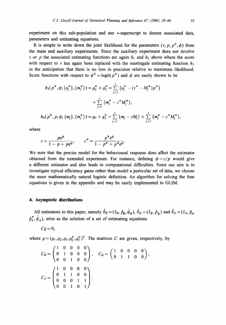
We note that the precise model for the behavioural response does affect the estimator obtained from the extended experiment. For instance, defining q~ = c / p would give a different estimator and also leads to computational difficulties. Since our aim is to investigate typical efficiency gains rather than model a particular set of data, we choose the more mathematically natural logistic definition. An algorithm for solving the four equations is given in the appendix and may be easily implemented in GLIM.

4. Asymptotic distributions

All estimators in this paper, namely 0o = (fB,/3B, q~B), 0~ = (f6, ~bo) and 0A = (fA,/3A,

/3A, q~A), arise as the solution of a set of estimating equations

Cg = O,

where g =(g l , , • Y g2, g3,g2 ,g3 ) • The matrices C are given, respectively, by

(1 o o o i) / oooo / C 8 = 0 1 0 0 , C ¢ = 1 1 0 0 '

0 0 1 0

CA =

( 000 ) 1 1 0 0 0 1 0 1 0

36 CZ Lloyd~Journal of Statistical Planning and Inference 67 (1998) 29~14

The asymptotic variance of these estimators follows from the theory of (martingale) estimating functions. A non-technical summary follows, avoiding the usual measure theoretic presentation for the sake of clarity. Let the data X have distribution depending on an unknown parameter 0 of dimension k. The data are 'filtered' into an increasing

sequence of subsets

X 1 c X 2 c . . . C X r = X ,

where C means the left-hand side is computable from the right-hand side. Often, Xj

will be the data collected up to a certain time j. For i = 1 . . . . . k suppose we have

functions

r oi(x, 0) = ~ o,Axj, 0)

j = l

satisfying

Ej_,(gij)=O, j = l . . . . . T

where Ej denotes expectation conditional on Xj. Then the vector of functions g = (gl . . . . . gk) T is called an unbiased (martingale) estimating function for 0.

Properties of the estimator 3 defined as the root of the estimating equation g = 0

depend on the matrices D and 2~ with entries

T

Dik =j=l ~ Ej-1 \ ~30k ] ' j=l

A minimal condition for consistency of 3 is that D is non-singular, i.e. that the gi are

linearly independent and that each gi depends on at least one component of 0. With this restriction the information in the estimating functions g is

I = DtZ- ID, (5)

where t denotes matrix transpose. Then often, 11/2(3-O) is asymptotically multivariate normal for large T, see Godambe and Heyde (1987). The main conditions are that (i) the mean derivative of certain combinations of the gi equal the derivative of the means, and (ii) that / /T converges in distribution to a positive random variable for large T. Then the inverse I may be used as the asymptotic variance of 0.

In our application the information in the estimating functions C9 is

Ic = ( C D ) t ( c z ~ c t )-1 CD.

There is no problem in the first condition since each of our estimating fimctions de- compose into products of functions of the parameters and functions of the data. The second condition is less straightforward. Notice that each of the estimating functions can be written as a double sum with T = vt terms. For instance,

g 2 = j = l i--1

CJ. Lloyd~Journal of Statistical Planning and Inference 67 (1998) 29-44 37

where j~j indicates that individual i is first captured on occasion j and Cij that in-

dividual i has been captured before occasion j . The mean derivative matrix CD and variance matrix CXC t are also double sums. Clearly, if v diverges and other parameters are held fixed then both these matrices increase like v and so I/T = t-lI/v converges. However, if v is fixed and t diverges this is not true. The problem is that eventually all individuals are captured and so, for instance, Ej- l ( f i j )=O and the terms added to D and S are zero. Nevertheless, before this limiting situation is reached, I will tend to increase with t. In summary the conditions for using I c 1 as the asymptotic variance is that Ic be large. In practice, this means T = vt is large but t is not so large that all the population is captured.

5. Computation of the information

The conditional expectation terms in D and Z are random, making comparison of the different designs dependent on the particular data set. However, these terms converge to their unconditional expectations provided that the Mj converge to their expectations. The conditions for this are identical to the conditions under which Ic/(vt) converges. In this case the statistics

t t (1 - p)P Mj --* v(t - P/p), ~ (v - Mj) -1 ~ (6)

j= l j= l vp(1 - P)

and substituting this in the expressions for I c I gives the asymptotic variance of ~ as the top left element. Let Q = I - P , q = l - p , D12--vtQp2/p and D32=vc(l - c ) ( t - P/p). Terms like D72 below indicate an identical expression to D12 but with auxiliary parameters replacing main parameters. Assuming that the weights wj sum to unity, explicit forms for the matrices D and 2~ with (6) substituted are 0) ° ° i / vPq 0 0 I D12 D22 0 0

D = D32 0 D 3 2 , - Y ' = , 0 0 0 3 2 0 . ( 7 )

1 0 0 D~2 0 0 0 D72/t* D12 ] o 0* o o 072 o 2/

Figs. 2 -4 describe the extent to which auxiliary experimentation can achieve the potential gains plotted in Fig. 1. In each case we imagine that v*= 10,50 or 100 individuals are separated from the population without preventing future behavioural response. A recapture experiment is performed on the sub-population with capture effort P * = 0.5 and t * : 10 occasions. Other values of P* and t* were tried but the precision of ~A is not greatly affected so long as P* is not too small. The asymptotic variance of the estimator ~* is computed by computing I c l assuming v - v * individuals in the main population and v* in the sub-population.

The vertical axis is the standard deviation of estimation divided by the true value of v. The upper solid line describes the estimator ~s and the lower solid line the estimator

38 C.J. Lloyd/Journal of Statistical Planning and Inference 67 (1998) 29-44

~o .~ Lom c~

o (5

.......... v *= lO

. . . . V*=50 V*= IO0

I I I I 50 100 500 1000

Fig. 2. Relative standard errors of fB (upper solid line), fO (lower solid line) and fA (broken lines) against mean number of captures, for three choices of v* (logarithmic scale on both axes, v = 500, q~ = 1 ).

~4,. The horizontal axis is the expected number of captures during the experiment. For fB and fO this is simply vpt. For the estimator fA this is ( v - v * ) p t + v * p * t * . This is

to compare the precision of estimation across the different designs for the equivalent capture effort/cost which is taken to be proportional to the number of captures. A

proper economic analysis would, o f course, likely produce a different measure. For a given total number of captures, the relative standard error is proportional to

v 1/2 while we have seen in Fig. 1 that the gains from knowing the behavioural pa- rameter q~ are largest when ~b is moderately large. The parameter values for (v, qS)

for Figs. 2 - 4 are, respectively, ( 5 0 0 , - 1 ) , (1000,0) and (5000,2). The distance be- tween the upper and lower solid curves describes the potential gains in knowing the behavioural parameter ~b. As expected, the plots show that this potential gain increases with increasing v and q~, at least so long as q~ is not too big. Notice that both axes are on logarithmic scale.

The extent to which fA achieves these potential gains is displayed by the curves plotted with broken lines. The effectiveness of the auxiliary designs is visually under- estimated, since the vertical axes are on the logarithmic scale. For instance, under the favourable conditions of Fig. 4, taking 100 individuals from 5000 for the sub-population and with a total o f 500 individuals captured over the entire experiment, the relative standard deviation is 150% for vB and 24% for VA. Under the less favourable conditions

C.J. Lloyd/Journal of Statistical Planning and Inference 67 (1998) 29-44 39

g

g "y,

"o ,2

~ o

o

I -!iii o I

I I I I 50 100 500 1000

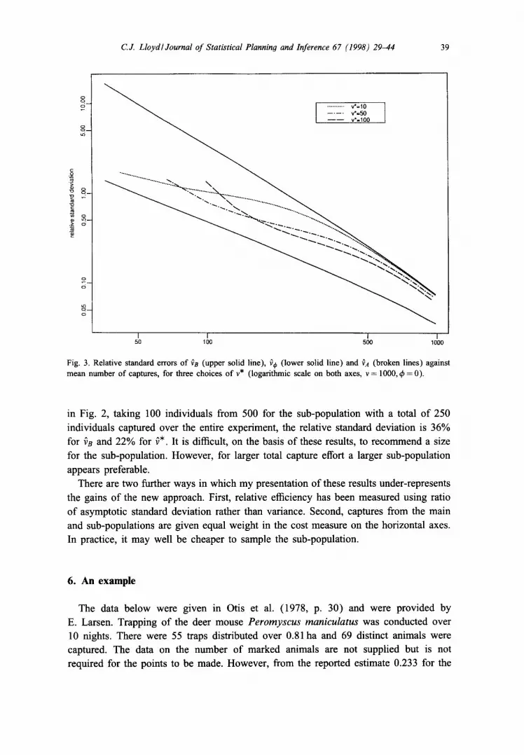
Fig. 3. Relative standard errors of ~B (upper solid line), ~ (lower solid line) and vA (broken lines) against mean number of captures, for three choices of v* (logarithmic scale on both axes, v = 1000, ~b = 0).

in Fig. 2, taking 100 individuals from 500 for the sub-population with a total o f 250

individuals captured over the entire experiment, the relative standard deviation is 36% for fn and 22% for f*. It is difficult, on the basis of these results, to recommend a size for the sub-population. However, for larger total capture effort a larger sub-population

appears preferable. There are two further ways in which my presentation of these results under-represents

the gains of the new approach. First, relative efficiency has been measured using ratio of asymptotic standard deviation rather than variance. Second, captures from the main and sub-populations are given equal weight in the cost measure on the horizontal axes.

In practice, it may well be cheaper to sample the sub-population.

6. An example

The data below were given in Otis et al. (1978, p. 30) and were provided by E. Larsen. Trapping of the deer mouse Peromyscus maniculatus was conducted over 10 nights. There were 55 traps distributed over 0.81 ha and 69 distinct animals were captured. The data on the number of marked animals are not supplied but is not required for the points to be made. However, from the reported estimate 0.233 for the

40 CJ. Lloydl Journal o f Statistical Planning and Inference 67 (1998) 29-44

o

o 5 -

o t6

°o_

o_ (5

o

o -

(:5

. . . . v'=50

. . . . -~" " ~ " " ' ~ ' - " ---k~" " ..... ~"

I I I I 5 0 1 0 0 5 0 0 .1000

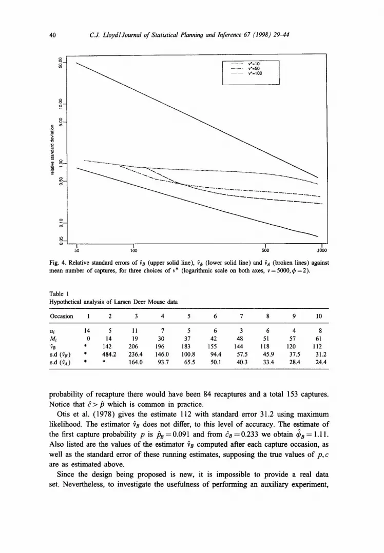
Fig. 4. Relative standard errors of fs (upper solid line), ~¢ (lower solid line) and va (broken lines) against mean number of captures, for three choices of v* (logarithmic scale on both axes, v = 5000, q~ =2).

Table 1 Hypothetical analysis of Larsen Deer Mouse data

Occasion 1 2 3 4 5 6 7 8 9 10

ui 14 5 11 7 5 6 3 6 4 8 Mi 0 14 19 30 37 42 48 51 57 61 vs * 142 206 196 183 155 144 118 120 112 s.d (vs) * 484.2 236.4 146.0 100.8 94.4 57.5 45.9 37.5 31.2 s.d (vA) * * 164.0 93.7 65.5 50.1 40.3 33.4 28.4 24.4

probabil i ty o f recapture there wou ld have been 84 recaptures and a total 153 captures.

Not ice that ~ > / 3 which is c o m m o n in practice.

Otis et al. (1978) gives the est imate 112 with standard error 31.2 us ing m a x i m u m

likelihood. The est imator fB does not differ, to this level o f accuracy. The est imate o f

the first capture probabil i ty p is /3 s = 0 . 0 9 1 and f rom ~s = 0 . 2 3 3 we obtain q~s = 1.11.

Also listed are the values o f the est imator f s computed after each capture occasion, as

wel l as the standard error o f these running estimates, supposing the true values o f p, c

are as es t imated above.

Since the design be ing proposed is new, it is impossible to provide a real data

set. Never theless , to invest igate the usefulness o f per forming an auxil iary exper iment ,

CJ. Lloyd~Journal of Statistical Planning and Inference 67 (1998) 29-44 41

imagine that the first 14 captured animals are an auxiliary population, still subject to behavioural response. For both the auxiliary and main populations, a recapture ex- periment is performed with t = t*, probability of first capture 0.091 and of recapture 0.233. While the required data to compute fA is not at hand, we can still compute the asymptotic standard error from equations (5, 7). The standard error of ~A is listed for t---2 . . . . . 9. The improvement comes from knowing the size of the auxiliary population, and the assumption that it is still subject to behavioural response. Better results again are obtained by concentrating extra effort on this population.

7. Simulation

The efficiency comparisons are based on asymptotic variance expressions for esti- mators under the competing designs. Extensive simulations of vs are already in the literature (Otis et al., 1978) and will not be repeated. It is worth repeating however that the probability that ~s is infinite can be appreciable and that even where it is small the skewness of the estimator is high and the variance, conditional on being finite, is typically much higher than predicted by asymptotics.

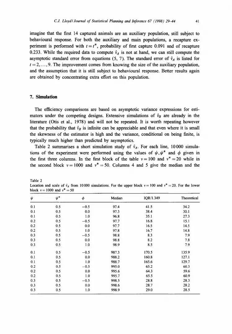
Table 2 summarises a short simulation study of fA. For each line, 10000 simula- tions of the experiment were performed using the values of ~k, ~k* and ~b given in the first three columns. In the first block of the table v = 100 and v* =20 while in the second block v = 1000 and v*= 50. Columns 4 and 5 give the median and the

Table 2 Location and scale of vA from 10000 simulations. block v = 1000 and v* = 50

For the upper block v = 100 and v* = 20. For the lower

~* q~ Median IQR/1.349 Theoretical

0.1 0.5 --0.5 97.4 41.5 34.2 0.1 0.5 0.0 97.3 38.4 30.1 0.1 0.5 1.0 96.8 35.1 27.3 0.2 0.5 --0.5 97.7 16.8 15.1 0.2 0.5 0.0 97.7 16.5 14.5 0.2 0.5 1.0 97.8 16.7 14.8 0.3 0.5 --0.5 98.8 8.3 7.9 0.3 0,5 0.0 98.8 8.2 7.8 0.3 0,5 1.0 98.9 8.5 7.9

0.1 0.5 --0.5 987.3 170.5 135.9 0.1 0,5 0.0 988.2 160.8 127.1 0.1 0,5 1.0 988.7 165.6 129.7 0.2 0,5 --0.5 995.0 65.2 60.3 0.2 0,5 0.0 995.6 64.3 59.6 0.2 0,5 1.0 995.7 65.5 60.9 0.3 0,5 -0 .5 998.5 28.8 28.3 0.3 0,5 0.0 998.6 28.7 28.2 0.3 0.5 1.0 998.9 29.0 28.5

42 C.J. Lloyd~Journal of Statistical Plannin# and Inference 67 (1998,) 29-44

interquartile range divided by 1.349. These robust measures suppress the effect of a small number of extremely large estimates which inevitably appear in such a large simulation. The last column has the asymptotic standard deviation computed using (5). The asymptotic standard error generally underestimates the true standard deviation, but the agreement improves as the standard error decreases. This is typical behaviour of recapture estimators.

8. Discussion

The primary assumptions underlying the analysis of the auxiliary experiment are (i) that the behavioural parameter is the same for the two populations, (ii) that v* is known, and (iii) that different efforts p and p* can be applied to the two populations.

The last requires physical separation of the two populations. If the populations are not separated then the design does not differ from standard mark recapture except that assumption (i) is made. Separation is important because it allows concentration of sampling effort on the auxiliary population whose size is known.

Achieving both (i) and (ii) requires v* individuals to be separated and counted without inducing the behavioural response. For animals with small ranges, one might 'fence off' a physical section of the environment followed by a non-invasive census. Or one might use a better (and more expensive) capture technique, followed by a period for the behavioural response to 'wear off'. In the latter case, why not use the better technique all the time? First it might be difficult and expensive, and waiting for the wear off period between each capture occasion could make the experiment time- consuming and violate population closure. Second, we have shown that capturing a single cohort without inducing behavioural response already produces large efficiency gains.

However, it is not suggested that this is always practical or that the commonly em- ployed but simplistic behavioural model is particularly realistic. We have mainly been using the model to investigate the efficiency of auxiliary experimentation per se, under disadvantageous conditions. For other models of behavioural response the same prac- tical difficulties may not arise. For instance, if one assumed that the same behavioural response (on some scale) occurs each time an individual is captured, then, so long as the model was correct, it should apply to the auxiliary population just as well as to the main population, without any special sampling technique. Indeed, it is strange that the behavioural reponse is not commonly modelled, for instance by a logistic regres- sion with some measure of the previous capture intensity as covariate. Fitting a correct model would certainly increase precision, even without auxiliary experimentation, and research on the efficiency of combining modelling with auxiliary experimentation is currently underway.

Finally, heterogeneous populations may also benefit from auxiliary experimentation. However, if the sub-population is simply sampled from the main population then the capture susceptibilities will be a biased sample from the distribution of susceptibilities

C.J. Lloyd~Journal of Statistical Planning and Inference 67 (1998) 29-44 43

across the main population; the analysis will involve some sampling theory and likely be more complicated. Another approach to heterogeneous populations is to measure covariates on individuals which hopefully predict their susceptibilities. Since the co- variates of uncaptured individuals are unmeasured, this leads to methods conditional on the event of capture at all, described by Huggins (1989).

Appendix

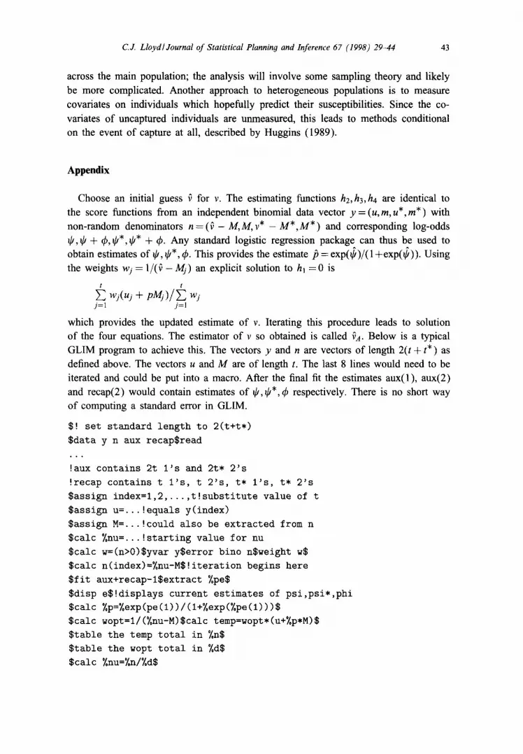
Choose an initial guess f for v. The estimating functions h2, ha, h4 are identical to the score functions from an independent binomial data vector y = (u, m, u* ,m*) with non-random denominators n = (f - M,M, v* - M * , M * ) and corresponding log-odds if, ff + ~b, qJ*, qJ* + ~b. Any standard logistic regression package can thus be used to obtain estimates of ~9, ~k*, ~b. This provides the estimate/3 = exp(~)/(1 +exp(~)) . Using the weights wj = 1 / ( f - Mj) an explicit solution to hi = 0 is

t t

wj(uj + p )/E w s j = l j = l

which provides the updated estimate of v. Iterating this procedure leads to solution of the four equations. The estimator of v so obtained is called ~A. Below is a typical GLIM program to achieve this. The vectors y and n are vectors of length 2(t + t*) as defined above. The vectors u and M are of length t. The last 8 lines would need to be iterated and could be put into a macro. After the final fit the estimates aux(l), aux(2) and recap(2) would contain estimates of ~O, ~b*, q~ respectively. There is no short way of computing a standard error in GLIM.

S! set standard length to 2(t+t*)

$data y n aux recapSread

!aux contains 2t l's and 2t* 2's

!recap contains t l's, t 2's, t* l's, t* 2's

Sassign index=1,2,...,t!substitute value of t

$assign u=... !equals y(index)

$assign M=... !could also be extracted from n

$calc ~,nu=... !starting value for nu

$calc w=(n>O)Syvar ySerror bino nSweight w$

$calc n(index)=~,nu-MS!iteration begins here

Sfit aux+recap-l$extract %pe$

$disp eS!displays current estimates of psi,psi*,phi

$calc %p=%exp (pe (1)) / ( l+~,exp (%pe (1) ) ) $

$calc wopt=l/(~,nu-M) $calc temp=wopt* (u+~.p*M) S

Stable the temp total in ~,n$

Stable the wopt total in %d$

Scalc %nu=7.n/%dS

44 C.J. Lloyd/Journal of Statistical Plannin9 and Inference 67 (1998) 29-44

References

Chaiyapong, Y., Lloyd, C.J., 1995. Minimum capture effort for recapture experiments with behavioural response. La Trobe University Research Report.

Chaiyapong, Y., Lloyd, C.J., 1996. Accurate inference for recaptta'e experiments with behavioural response. J. Statist. Comput. Sim. 56, 97-115.

Darroch, J.N., 1958. The multiple-recapture census. I. Estimation of a closed population. Biometrika 45, 343-359.

Huggins, R.M., 1989. On the statistical analysis of capture experiments. Biometrika 76, 133-140. Godambe, V.P., Heyde, C.C., 1987. Quasi-likelihood and optimal estimation. Int. Statist. Rev. 55, 231-244. Laska, F.M., Meisner, M., 1993. A plant-recapture method for estimating the size of a population from a

single sample. Biometrics 49, 209-220. Lloyd, C.J., 1994. Efficiency of martingale methods in recapture studies. Biometrika 81, 305-315. Lloyd, C.J., Yip, S.F., 1991. A unification of inference from capture-recapture studies through martingale

estimating functions. In: V.P. Godambe (Ed.), Estimating Functions. Clarendon Press, Oxford, pp. 65-88. Mills, H.D., 1970. On the statistical validation of computer programs IBM FSD Rep. Otis, D.L., Burnham, K.P., White, G.C., Anderson, D.R., 1978. Statistical inference from capture data on

closed animal populations. Wildlife Monographs 62, 1-135. Seber, G.A.F., 1982. Estimation of Animal Abundance and Related Parameters, 2nd ed., Griffin, London. Seber, G.A.F., Whale, J.F., 1970. The removal method for two and three samples. Biometrics 26, 393-400.