Focused information criterion for capture-recapture models for closed populations (short title: FIC for closed capture-recapture models)

Focused information criterion

for capture-recapture models for closed populations

Francesco Bartolucci∗† and Monia Lupparelli∗‡

November 16, 2007

Abstract

We propose a criterion for selecting a capture-recapture model for closed populations

which follows the basic idea of the Focused Information Criterion (FIC) of Claeskens

and Hjort (2003). The proposed criterion aims at selecting the model which, among

the available models, leads to the smallest Mean Squared Error (MSE) of the resulting

estimator of the population size and is based on an index which, up to a constant

term, is equal to the asymptotic MSE of the estimator. Two alternative approaches

to estimate this FIC index are proposed. We also deal with multimodel inference; in

this case, the population size is estimated by using a weighted average of the estimates

coming from different models, with weights chosen as to minimize the MSE of the

resulting estimator. The proposed model selection approach is compared with more

common approaches through a series of simulations performed along the same lines

as Stanley and Burnham (1998). It is also illustrated by an application based on a

dataset coming from a live-trapping experiment.

Key words: AIC, CAIC, conditional maximum likelihood estimation, model selection,

multimodel inference.

∗Dipartimento di Economia, Finanza e Statistica, Universita di Perugia, 06123 Perugia, Italy.†email: [email protected]‡email: [email protected]

1

1 Introduction

In many contexts, the estimation of the size of a certain population, such as that of ani-

mals living in a certain region or that of people suffering from a certain disease, is carried

out on the basis of capture-recapture data; for a review see Yip et al. (1995a,b), Schwarz

and Seber (1999), Borchers et al. (2004) and Amstrup et al. (2005), among others. These

data are typically collected by means of a series of trapping experiments or by matching

the information contained in two or more administrative lists and consist of sequences of

binary outcomes that, for each subject observed at least once, indicate if the subject has

been or not “captured” at a given occasion. A wide variety of models is now available for the

analysis of data like these. It ranges from very simple models, such as that assuming that

capture probabilities are equal across subjects and occasions, to very sophisticated models

which take into account all the factors that may affect these probabilities, i.e. time, behavior

and heterogeneity (Otis et al., 1978). Since the estimate of the population size crucially de-

pends on the adopted model, model selection is a fundamental issue in the capture-recapture

context.

As in many other fields, the Akaike Information Criterion (AIC, Akaike, 1973) is one of

the most used criteria for model selection also in this field. This criterion is usually preferred

for its simple use and nice interpretation in terms of distance between the true model, i.e.

the data generating model, and the assumed model. The quality of the inference on the

population size, when the model is selected with AIC, was studied by simulation by Burnham

et al. (1995) and Stanley and Burnham (1998). It results that this criterion usually leads

to selecting a model that, in the class of available models, is a good compromise between

the largest model, which guarantees a small bias of the resulting estimator of the population

size, and the smallest model, which guarantees a small variance of this estimator. These

authors also considered other selection criteria, such as AICc and CAIC, which are versions

of AIC based on a penalization term taking the sample size also into account. These selection

criteria perform better than AIC in certain circumstances. Finally, they considered a form

of multimodel inference in which the population size is estimated by a weighted average of

2

the estimates coming from different models, with weights which are simply computed on the

basis of the AIC, AICc or CAIC index; for a general description of this type of inference see

Buckland et al. (1997) and Burnham and Anderson (2002, Ch. 4). It turns out that the

average estimator is usually more efficient than the corresponding single-model estimator.

An important point to underline is that the AIC, as well as the other selection criteria

mentioned above, are aimed at finding the model which, among the available models, provides

the best approximation of the true model. However, it is not ensured that such a model also

guarantees the smallest estimation error of the population size. In fact, for the same data, we

can usually find two or more models which have very close values of the AIC index, but lead

to very different estimates of the population size. To this regard, the examples provided by

Agresti (1994) and Fienberg et al. (1999) are illuminating. For instance, among the models

considered by Fienberg et al. (1999, Sec. 5.2) for the analysis of a capture-recapture dataset

concerning 2,069 cases of diabetes in an Italian region, there are two models for which the

difference in terms of AIC index is around 0.6, but one leads to an estimate of the population

size equal to 2,381, whereas the other model leads to an estimate of 7,796.

Recently, Claeskens and Hjort (2003) proposed a model selection strategy to be used

when the main interest is in estimating a certain parameter, rather than on representing

adequately the data generating mechanism. This criterion, known as Focused Information

Criterion (FIC), is based on an index that, up to a constant term, is equal to the asymptotic

Mean Squared Error (MSE) of the estimator of the parameter of interest under the model

to which it is referred. This index is developed by exploiting certain asymptotic results of

Hjort and Claeskens (2003) concerning the properties of maximum likelihood estimators in

the presence of misspecification. These results, however, are not directly applicable to the

capture-recapture context, in particular when the conditional maximum likelihood (CML)

approach of Sanathanan (1972) is used to estimate a closed-population model, i.e. a model

assuming that the population size is constant during the period of observation (Borchers

et al., 2004). Note that the inferential framework dealt with in this paper is different from

the traditional one, since, in our context, the sample size is a random quantity, whereas the

(unknown) population size is a fixed quantity. The asymptotic theory is then developed for

3

the latter tending to infinity. This is the main reason why the results of Hjort and Claeskens

(2003) are not directly applicable to our context.

In this paper, we extend the main results of Hjort and Claeskens (2003) to the case in

which a closed-population model is estimated with the CML approach and derive a FIC

index for the resulting estimator. We also introduce two estimators of this index, the first

of which recalls that proposed by Claeskens and Hjort (2003), whereas the second follows a

new idea. We also deal with the estimation of the population size on the basis of a weighted

average of the estimates coming from different models, with weights chosen by minimizing

a function which provides a measure of error of the resulting estimator of the population

size. This criterion for choosing the weights follows a different conception with respect to

that used in connection with AIC and similar selection criteria and recalls that exploited by

Hansen (2007) in a different context. The approach proposed here is illustrated by a series

of simulations performed along the same lines as Stanley and Burnham (1998).

The paper is organized as follows. In Section 2 we review the CML approach for the

estimation of a closed-population model and we recall the main asymptotic properties of

this approach when the assumed model holds. In Section 3 we study the same properties

when the model is misspecified and then we derive an expression for the asymptotic MSE

of the estimator of the population size and a FIC index for this estimator and its weighted

average version. On the basis of these results, in Section 4 we deal with model selection and

multimodel inference on the population size. The approach is illustrated by a simulation

study and an application involving a dataset coming from a live-trapping experiment, the

results of which are reported in Sections 5 and 6. Finally, in Section 7 we draw the main

conclusions and we outline some possible extensions of the proposed approach.

2 Conditional inference for closed-population models

Let N denote the unknown population size, let J denote the number of capture occasions

and let p(r) denote the probability of the capture configuration r = ( r1 · · · rJ ), where

rj is a binary variable equal to 1 if a subject is captured at the j-th occasion and to 0

4

otherwise. Also let m = 1− p(0) be the probability of being captured at least once and let

q(r) = p(r)/m be the conditional probability of the capture configuration r for a subject

captured at least once. Finally, for every r 6= 0, y(r) denotes the frequency of the subjects

with capture configuration r so that n =∑

r 6=0 y(r) is the sample size. We have to stress

that n is a random variable whose distribution depends on the capture probabilities. On

the other hand, N is a fixed quantity and the asymptotic theory that follows is developed

for this quantity tending to infinity, not for n tending to infinity as in standard inferential

contexts.

To estimate N on the basis of the frequencies y(r), we must assume a model on the

probabilities p(r). In this paper, we suppose that a collection M of models is available. The

largest model in this class, referred to as full model, assumes that p(r) = f(r; β,γ) for a

suitable function f(·) and where β and γ are two vectors of parameters to be estimated.

The smallest model in class M, referred to as null model, is a particular case of the full

model in which γ = γ0, where γ0 is a fixed parameter vector. Between the full and the null

models, there exist models in which only certain elements of γ are fixed at the corresponding

elements of γ0 and the other ones have to be estimated, i.e. γ = (γ ′S ,γ′S,0

)′ for a subset S of

F = 1, . . . , c, with c denoting the size of γ and S its complement. Each model in M may

consequently be denoted by MS and its parameter vector by θS = (β′,γ ′S)′, whereas pS(r),

qS(r) and mS denote the corresponding probability functions defined as above. It has to be

clear that these are functions of θS . Finally, note that MF obviously corresponds to the full

model, whereas M∅ corresponds to the null model.

In the following, we show how the parameters of each model MS , and consequently N ,

may be estimated by the CML approach. We also discuss model selection.

2.1 Estimation of the model parameters and population size

In the CML approach, the parameter vector θS of model MS is estimated by maximizing

the conditional log-likelihood of the observed capture configurations given the sample size n.

This function may be expressed as

`(θS) = y′ log(qS),

5

where qS denotes the column vector with elements qS(r) for every r 6= 0 and y denotes the

corresponding vector with elements y(r). Both vectors have 2J − 1 elements.

The Expectation-Maximization (EM) algorithm (Dempster et al., 1977) is normally used

to maximize `(θS). It consists of alternating the following steps until convergence:

• E-step: given the current estimate of θS , denoted by θS , compute the expected value

of the number of subjects which have not been captured as

y(0) = n1− mS

mS;

• M-step: update the estimate of θS by maximizing the conditional expected value of

the complete log-likelihood given y and θS . This log-likelihood may be expressed as

˜∗(θS ; θS) = y(0) log(1−mS) + y′ log(pS),

where pS denotes the vectors with elements pS(r) for every r 6= 0. Typically, ˜∗(θS ; θS)

is maximized by means of a Newton-Raphson algorithm based on the following first

derivative vector and second derivative matrix

∂ ˜∗(θS ; θS)∂θS

= − y(0)

1−mS

∂mS∂θS

+∂p′S∂θS

diag(pS)−1y,

∂2 ˜∗(θS ; θS)∂θS∂θ′S

= − y(0)

(1−mS)2

∂mS∂θS

∂mS∂θ′S

− y(0)

1−mS

∂2mS∂θS∂θ′S

+

−∂p′S∂θS

diag(y)diag(pS)−2∂pS

∂θ′S+

∑

r 6=0

y(r)

pS(r)

∂2pS(r)

∂θS∂θ′S.

The value of θS at convergence of the EM algorithm, which we take as the CML estimate

of θS , is denoted by θS . We then estimate the population size under model MS as NS =

n/mS .

2.2 Asymptotic properties under the assumed model

First of all consider that the score vector for model MS may be expressed as

s(θS) =∂`(θS)∂θS

=∂q′S∂θS

diag(qS)−1y.

6

Since y has variance equal to NΩS , with ΩS = diag(pS) − pSp′S , the Fisher information

matrix, i.e. the variance-covariance matrix of s(θS), may be expressed as

F (θS) = N∂q′S∂θS

diag(qS)−1ΩSdiag(qS)

−1 ∂qS∂θ′S

= mSN∂q′S∂θS

diag(qS)−1 ∂qS

∂θ′S.

This matrix, evaluated at θS,0 = (β′0, γ′S,0)

′, the true value of the parameter vector θS , is

denoted by F S,0 and JS,0 = F S,0/N is the corresponding average information matrix.

Now consider the following assumptions that in our approach need to hold for each model

MS in class M:

A1. for every capture configuration r, pS(r) is strictly positive and admits continuous

first-order derivatives at every admissible value of θS ;

A2. for any ω > 0, it is possible to find an ε > 0 such that

inf|θS−θS,0|>ω

∑

r 6=0

qS,0(r) logqS,0(r)

qS(r)> ε,

with qS,0(r) denoting the probability qS(r) evaluated at θS,0;

A3. the Jacobian of ( pS(0) p′S ) with respect to θS is of full rank.

Note that A1 is a standard regularity condition on the function pS(r), A2 is a strong iden-

tifiability condition (see also Rao, 1965, Sec. 5e.2) expressed directly on the conditional

probabilities qS(r) and A3 implies that the Fisher information matrix at θS,0, F S,0, is of full

rank. It is worth noting that, if the conditions above hold for the full model in class M,

then they hold for each submodel MS in the same class.

Under assumptions A1, A2 and A3, Theorem 2 of Sanathanan (1972) implies that:

• θSp−→ θS,0 and

√N(θS − θS,0)

d−→ N (0,J−1S,0)

• NS/Np−→ 1 and (NS −N)/

√N

d−→ N (0, η2S)

for each model MS , with

η2S =

1−mS,0

mS,0

+1

m2S,0

∂m(θS,0)

∂θ′SJ−1S,0

∂m(θS,0)

∂θS. (1)

7

We recall thatp−→ means convergence in probability and

d−→ means convergence in distri-

bution as N →∞. Moreover, in the above expression, we use

∂m(θS,0)

∂θS

to denote the derivative of mS with respect to θS evaluated at θS,0. A similar convention is

used to denote a derivative of a function of θS evaluated at θS .

The asymptotic results above imply that we can compute the standard errors for θS and

NS from an estimate of JS,0. To this aim consider the following assumption:

A4. for every capture configuration r, pS(r) admits continuous second-order derivatives at

every admissible value of θS .

Under A4, F (θS) is equal to the (unconditional) expected value of

H(θS) = − ∂2`(θS)∂θS∂θ′S

=∂q′S∂θS

diag(y)diag(qS)−2 ∂qS

∂θ′S−

∑r

y(r)

qS(r)

∂qS(r)

∂θS∂θ′S,

which is the observed information matrix. We also have that ‖H(θS)/N − JS,0‖ p−→ 0 and

then JS,0 may be consistently estimated by

JS = H(θS)/NS . (2)

The standard error for θS directly follows from the inverse of H(θS); because of (1), the

standard error for NS is given by√

NS1− mS

mS+

N2S

m2S

∂m(θS)∂θ′S

H(θS)−1∂m(θS)

∂θS.

2.3 Information criteria for model selection

One of the most used criteria for selecting a model for the analysis of a capture-recapture

dataset is the AIC (Akaike, 1973). It is based on an index which provides a measure of the

distance between the assumed model MS and the true model and is defined as

AICS = −2`(θS) + 2kS ,

where kS is the number of the model parameters. Consequently, among the available models,

we prefer the one with the smallest value of this index.

8

Other criteria for model selection are available in the literature which may be seen as

versions of the above one; for a review in the capture-recapture context see Burnham et al.

(1995) and Stanley and Burnham (1998). Among these criteria, it is worth mentioning those

referred to as AICc and CAIC which are based on the indices

AICc,S = AICS +2kS(kS + 1)

n− kS − 1,

CAICS = −2`(θS) + kS [log(n) + 1],

which make use of a penalization term taking the sample size into account.

In the capture-recapture context, the model selected according to one of the above criteria

is used to obtain an estimate of the population size (single-model inference). A different ap-

proach is that based on model averaging (multimodel inference) which consists of estimating

the population by

Nw =∑S

wSNS , (3)

where∑

S denotes the sum over all the models in M and

wS =exp(−AICS/2)∑S′ exp(−AICS′/2)

(4)

is the AIC-weight for model MS . A similar estimator may be based on the other selection

criteria mentioned above. In particular, the formula for computing AICc and CAIC-weights

is the same as (4), with AICS substituted by AICc,S and CAICS , respectively. For a general

discussion on this type of inference see Buckland et al. (1997).

3 Asymptotic properties under the true model

Similarly to Claeskens and Hjort (2003) and Hjort and Claeskens (2003), we now assume

that the full model holds with β = β0 and γ = γ0 + δ/√

N , where δ denotes a fixed vec-

tor of suitable dimension. This model is referred to as true model and the corresponding

probability of the capture configuration r is denoted by ptrue(r) = f(r; β0,γ0 + δ/√

N).

These probabilities are collected in the vector ptrue for every r 6= 0. We also denote by

p0(r) = f(r; β0, γ0) the probability of r when β = β0 and γ = γ0 and by p0 the corre-

sponding probability vector. Similarly, we use q0(r) to denote the conditional probability

9

q(r) under this model, q0 to denote the corresponding probability vector and m0 to denote

the probability of being captured at least once.

Within this framework, we first study the asymptotic properties of the CML estimator of

θS , θS , and those of the corresponding estimator of N , NS . We then consider the asymptotic

properties of the estimator Nw.

3.1 Model parameters estimator

Let f = y/N be the vector of the relative frequencies of all capture configurations r 6= 0

and consider the following assumption:

A5. for every capture configuration r,

ptrue(r) = p0(r) +∂p0(r)

∂γ ′δ/√

N + O(N−1).

Under this assumption, the Central Limit Theorem implies that

√N(f − p0)

d−→ N(

∂p0

∂γ ′δ,Ω0

), (5)

as N → ∞, where Ω0 = diag(p0) − p0p′0. On the basis of this result we prove Theorem 1

below, where we use the following decomposition of the average information matrix under

the full model

JF ,0 =

(J00 J01

J01 J11

)

and P S denotes the block of rows of an identity matrix of size c such that γS = P Sγ. We

also recall that convergence in probability and distribution are for N →∞.

Theorem 1 Under the true model and provided that assumptions A1, A2, A3 and A5 hold,

for each model MS

• θSp−→ θS,0

• √N(θS − θS,0)d−→ N

[J−1S,0

(J01

P SJ11

)δ,J−1

S,0

].

Proof. See Appendix A1.

10

3.2 Population size estimator

Let

TS =NS −N√

N

and note that this quantity may also be expressed as

√N

(1′fmS

− 1

). (6)

The following Theorem holds.


for each model MS

• NS/Np−→ 1

• TSd−→ N (µS , σ2

S),

where

µS =1

m0

b′Sδ and σ2S =

1−m0

m0

+1

m20

∂m(θS,0)

∂θ′SJ−1S,0

∂m(θS,0)

∂θS,

with

bS =

[∂m0

∂γ ′− ∂m(θS,0)

∂θ′SJ−1S,0

(J01

P SJ11

)]′. (7)


This Theorem implies that the asymptotic MSE of TS may be expressed as

MSE(TS) = µ2S + σ2

S =1−m0

m0

+ FIC(TS),

with

FIC(TS) =1

m20

b′Sδδ′bS +1

m20

∂m(θS,0)

∂θ′SJ−1S,0

∂m(θS,0)

∂θS. (8)

It is worth noting that the asymptotic MSE of TS is equal to the index FIC(TS) plus a

term which is constant with respect to S. Therefore, as suggested by Claeskens and Hjort

(2003), it is reasonable to choose the model with the smallest value of this index, once it

has been properly estimated (see Section 4). Also note that the above formula for FIC(TS)

does not closely resemble the general formula provided by Claeskens and Hjort (2003). The

11

latter, however, is based on certain simplifications which we do not consider since they do

not affect the model selection strategy and are not so relevant in the present context.

Now consider the average estimator Nw defined in (3) in the case in which the weights

wS are a priori fixed. Let

Tw =Nw −N√

N

which may also be expressed as

√N

(∑S

wS1′fmS

− 1

).

The following Theorem holds, where w denotes a column vector with elements wS for every

model MS .


• Nw/Np−→ 1

• Twd−→ N (µw, σ2

w),

with

µw =1

m0

w′Bδ and σ2w =

1−m0

m0

+1

m20

w′CJF ,0C′w,

where B is a matrix with rows b′S and C is a matrix with rows c′S for every model MS, with

b′S defined in (7) and

cS =

[∂m(θS,0)

∂θ′SJ−1S,0

(I O

O P S

)]′.


From the above expression, we find that the asymptotic MSE of Tw may be expressed as

MSE(Tw) = µ2w + σ2

w =1−m0

m0

+ FIC(Tw),

with

FIC(Tw) =1

m20

w′Bδδ′B′w +1

m20

w′CJF ,0C′w. (9)

In the following, we show how to estimate FIC(Tw) and suggest an optimal procedure

for choosing w. This procedure is based on a different idea with respect to the standard

procedure used in connection with AIC and similar selection criteria.

12

4 Proposed model selection strategy

We now introduce an estimator of FIC(TS) which follows the basic idea of that of Claeskens

and Hjort (2003). We then discuss an alternative estimator of the same quantity based on a

different approach. Finally, we deal with estimation of FIC(Tw) and multimodel inference

on the population size.

4.1 Single-model inference

First of all note that, if A4 holds, we can consistently estimate all the quantities involved in

(8), with the exception of the matrix δδ′. Let

mF =∂m(θF)

∂θF

and partition this vector into the subvectors m1, referred to the parameters β, and m2,

referred to the parameters γ. We then have that

mS =

(m1

P Sm2

)

is a consistent estimator of the derivative of m(θS,0) with respect to θS and

bS =

[m′

2 − m′SJ

−1

S

(J01

P SJ11

)]′(10)

is a consistent estimator of bS , where J01 and J11 are suitable blocks of JF , with the latter

defined according to (2). Also JS,0 may be consistently estimated by using a suitable block

of JF , denoted in this case by JS .

To derive an estimator of δδ′, we rely on the Lemma below which directly follows from

Theorem 1 considering that NF/Np−→ 1 as N →∞.

Lemma 1 Under the true model and provided that assumptions A1, A2, A3 and A5 hold,

√NF(γF − γ0)

d−→ N (δ,K),

with K denoting the block of J−1F ,0 corresponding to J11.

13

This implies that an asymptotically unbiased estimator of δδ′ is

NF(γF − γ0)(γF − γ0)′ − K,

with K taken from J−1

F . By substituting the above expression into (8) and recalling the

definition of NF , we obtain an estimator of FIC(TS) which is given by

F IC(TS) =n

m3F

b′S(γF − γ0)(γF − γ0)

′bS +1

m2F

m′SJ

−1

S mS − 1

m2F

b′SKbS .

Note that, in the formula above, the quantities m0, bS and JS,0 are estimated by using the

CML estimator θF under the full model, but they could also be consistently estimated on

the basis of the CML estimator θ∅ under the null model (see Claeskens and Hjort, 2003).

An alternative estimator of FIC(TS), which has a nice interpretation, may be built as

follows. Let

DS =NS − NF√

NF

and consider the following Theorem.


DSd−→ N (νS , τ 2

S), with

νS =1

m0

b′Sδ and τ 2S =

1

m20

[∂m(θF ,0)

∂θ′FJ−1F ,0

∂m(θF ,0)

∂θF− ∂m(θS,0)

∂θ′SJ−1S,0

∂m(θS,0)

∂θS

].


Since νS = µS , we propose to estimate FIC(TS) with

F IC∗(TS) = D2

S − τ 2S + σ2

S =(NS − NF)2

NF− 1

m2F

m′F J

−1

F mF +2

m2F

m′SJ

−1

S mS ,

where by σ2S we mean an estimate of σ2

S − (1−m0)/m0.

Regardless of the estimator used for FIC(TS), we suggest to select the model with the

smallest estimate of this index and then taking the corresponding estimate of N . In the

following, this selection criterion will be indicated by FIC when it is based on the estimator

F IC(TS) and by FIC∗ when it is based on the alternative estimator F IC∗(TS). It may

obviously happen that FIC and FIC∗ do not lead to choosing the same model.

14

4.2 Multimodel inference

Given (9), we derive a first estimator of FIC(Tw) which closely recalls the structure of the

estimator F IC(TS) derived above. This estimator has the following structure

F IC(Tw) =n

m3F

w′B(γ − γ0)(γ − γ0)′B

′w − 1

m2F

w′BKB′w +

1

m2F

w′CJFC′w, (11)

where B is made of rows b′S defined in (10) and C is a matrix with rows c′S , with

cS =

[m′

SJ−1

S

(I O

O P S

)]′.

We can use an alternative estimator based on the asymptotic properties of

Dw =Nw − NF√

NF=

∑S

wSDS .


Dwd−→ N (νw, τ 2

w), with

νw =1

m0

w′Bδ and τ 2w =

1

m20

w′EJF ,0E′w,

where E is a matrix with rows e′S for every model MS , where

eS =

[∂m(θF ,0)

∂θ′FJ−1F ,0 −

∂m(θS,0)

∂θ′SJ−1S,0

(I O

O P S

)]′.


From this result, we have that FIC(Tw) may be estimated by

F IC∗(Tw) = D2

w − τ 2w + σ2

w = D2w − 1

m2F

w′EJFE′w +

1

m2F

w′CJFC′w, (12)

with σ2w denoting the estimator of σ2

w − (1 −m0)/m0 and E denoting a matrix with rows

e′S , where

eS =

[m′

F J−1

F − mSJ−1

S

(I O

O P S

)]′.

Regardless of the estimator used for FIC(Tw), we suggest to choose the vector of weights

w by minimizing the corresponding expression, which is of type (11) or (12), under the

constraints wS > 0, ∀S, and∑

S wS = 1; see also Hansen (2007). This optimization may be

15

performed by iterative algorithms which are available in most statistical and mathematical

packages. We suggest to initialize these algorithms by using CAIC-weights, since these

weights usually represent a good solution in terms of efficiency of the estimator of N . The

weights obtained from this optimization are used to compute a multimodel estimate of N

on the basis of (3) and, in the following, are indicated by FIC or FIC∗-weights according to

which estimator is chosen for FIC(Tw).

5 Simulation study

In order to compare the model selection criteria illustrated above with those based on AIC

and CAIC indices, we carried out a simulation study along the same lines as Stanley and

Burnham (1998). In the following, we illustrate the class of models considered in the study,

the simulation design and then the results we obtained.

5.1 A class of models for capture-recapture data

The full model in the class we considered allows for heterogeneity, time and behavior effects

on the capture probabilities. Using a notation taken from Otis et al. (1978), this model is

then of type Mhtb; see also Agresti (1994), Pledger (2000) and Dorazio and Royle (2003). The

heterogeneity effect is introduced via a random effect z having standard normal distribution.

Therefore, the model assumes that, given this random effect and for any j > 1, rj depends

on r1, . . . , rj−1 only through cj−1, where cj−1 is a dummy variable equal to 1 if the subject

has already been captured (i.e.∑

h<j rh > 0) and to 0 otherwise. This implies that

pF(r) =

∫

RpF(r|z)φ(z)dz, (13)

where

pF(r|z) =∏

j

λF(j|z, cj−1)rj [1− λF(j|z, cj−1)]

1−rj

and λF(j|z, cj−1) denotes the probability of being captured at the j-th occasion given z and

cj−1. Moreover, φ(z) denotes the density function of the standard normal distribution. The

16

model also assumes that

logλF(j|z, cj−1)

1− λF(j|z, cj−1)= β1 + zβ2 + t′jγ1 + cj−1γ2,

with c0 ≡ 0 and where tj is a (J − 1)-dimensional column vector of all zeros, apart form its

(j−1)-th element that, when j > 1, is equal to rj. In this way, the parameters in γ1 measure

the differential effect of each capture occasion with respect to the first occasion (time effect),

whereas γ2 measures the effect of a previous capture (behavior effect). Moreover, β1 is the

intercept and β2 is a scale parameter for the random effect (heterogeneity effect).

Several submodels may be conceived by setting to 0 suitable parameters of the full model.

Using the notation of Otis et al. (1978), these models may be indicated by Mtb, Mhb, Mht,

Mb, Mt, Mh, M0. The first model does not consider the heterogeneity effect, the second

does not consider the time effects and so on. Therefore, the last model does not consider

any of the mentioned effects. Estimation of each model may be carried out by using the EM

algorithm described in Section 2. Technical details useful for its implementation are given

in Appendix A2. In our implementation, the integral in (13) is computed by a quadrature

method based on a suitable grid of points.

Note that the application of our approach is made difficult by the fact that the conditions

on which it is based do not hold. This is because, in order to ensure identifiability and to

make possible that the full model specifies into a model without heterogeneity, we require

β2 > 0 and then the range of the admissible values of this parameter is not an open set.

In order to circumvent this difficult we apply FIC and FIC∗ (also in the case of multimodel

inference) as follows:

• We first test the hypothesis H0 : β2 = 0 (absence of heterogeneity) by a likelihood ratio

statistic between models Mhtb and Mtb; this statistic has null asymptotic distribution

of type χ21/2.

• If H0 is rejected, we restrict our attention only to the models including heterogeneity

effect so that it is possible to exclude from the parameter space the points with β2 = 0

and then the conditions on which our approach is based hold. The parameter vector

of the full model Mhtb is θF = (β′, γ ′)′, with β = (β1, β2)′ and γ = (γ ′1, γ2)

′. The

17

submodels we consider are Mhb, Mht and Mh. In our notation, these are indicated by

MS with, respectively, S = J, S = 1, . . . , J − 1 and S = ∅.

• If H0 is not rejected, we only consider models without heterogeneity effect. The full

model is in this case Mtb with parameter vector θF = (β, γ ′)′, where β = β1. The

corresponding parameter space is RJ and then the conditions on which our approach

is based hold. In this case, the submodels we consider are Mb, Mt and M0, which may

also be indicated by MS with S again defined as S = J, S = 1, . . . , J − 1 and

S = ∅, respectively.

5.2 Simulation design

For N = 200, 400 and J = 5, 7, we drew 1,000 samples from the full model Mhtb with

β2 = 0, 0.5, parameters in γ1 generated, for every sample, from the distribution N(0, σ2γ1

),

σ2γ1

= 0, 0.1, and γ2 = −0.5, 0, 0.5. Note that letting β2 = 0 is equivalent to removing

the heterogeneity effect from Mhtb, letting σ2γ1

= 0 is equivalent to removing the time

effect and letting γ2 = 0 is equivalent to removing the behavior effect. Therefore, when

β2 = σ2γ1

= γ2 = 0, model M0 results. Overall, we considered 48 scenarios corresponding

to two choices for J , two for N and twelve for the model parameters. Under each scenario,

the intercept β1 is chosen in order to have an expected sample size close to the 75% of the

population size. We then set β1 = −1.1 when J = 5 and β1 = −1.5 when J = 7.

For each generated sample, we fitted all the available models and we took, as estimate of

N , the one computed on the basis of the model selected with AIC, CAIC, FIC (based on the

estimator F IC(TS)) and FIC∗ (based on the estimator F IC∗(TS)). Note that, taking the

structure of the parameter space into account, the last two criteria are applied as described

at the end of the previous section. To assess the quality of the multimodel inference proposed

here, for each sample we also computed the weighted average estimate of N based on AIC,

CAIC, FIC and FIC∗-weights. In this way we considered height different estimators of N .

Note that we did not consider AICc because, according to Stanley and Burnham (1998), the

estimator of N based on this criterion performs very closely to that based on AIC.

18

For each estimator of N described above, we computed the Relative Mean Squared Error

(RMSE) as

1

1000

1000∑

h=1

(N (h) −N

N

)2

,

where N (h) is the estimate obtained from the h-th simulated sample. The results are dis-

played in Tables 1 to 4 which also show the RMSE of NF (the estimator of N based on

the full model Mhtb) together with the average percentage of captured population (CP), the

percentage of anomalous samples (RS) and the percentage of times the test of the hypothesis

of absence of heterogeneity (H0 : β2 = 0) is rejected (ET). In particular, RS is the percentage

of samples for which the maximum among the estimates of N obtained from Mhtb, Mhb, Mht

and Mh (when absence of heterogeneity is rejected) or the maximum among those obtained

from Mtb, Mb, Mt and M0 (when absence of heterogeneity is not rejected) is larger than

four times n. These samples are discharged and regenerated within the simulation, since

they lead to an unrealistic estimate of N . Note that procedures like this are common to

other simulation studies performed in the capture-recapture literature, as the one of Stanley

and Burnham (1998). They, in particular, adopted a procedure which discharges samples

whenever at least one of the estimates of N is greater than three times the true value of this

parameter. However, we consider our procedure more realistic, since it does require to know

the true population size.

5.3 Results

We first consider the results in Tables 1 and 2 of the simulations carried out in absence of

heterogeneity (β2 = 0). The first of these tables is referred to the case of J = 5 trapping

occasions. We can observe that, in terms of RMSE, FIC∗ is the best criterion for 9 of the

12 scenarios considered in this table. For the remaining 3 scenarios (corresponding to the

generating models M0 and Mb, which have not a high level of complexity), FIC∗ is the second

best criterion. Moreover, FIC results to be the second best criterion 7 times on 12. A similar

pattern is observed for J = 7 (see Table 2). In this case FIC∗ is the best criterion 8 times

on 12 and the second best for the 4 remaining times. FIC is second best criterion 7 times

19

on 12. Overall FIC and FIC∗ behave much better than AIC and CAIC and the advantage

is slightly more evident with N = 200 than with N = 400.

On the basis of Tables 1 and 2, we can draw similar conclusions for what concerns

multimodel inference. In particular, the average estimators of N based on FIC∗-weights is

the best, in terms of RMSE, 8 times on 12 when J = 5 and when J = 7. In the remaining

cases (essentially when samples are generated from models M0 and Mb), it is the second best

multimodel estimator of N . Moreover, the average estimators of N based on FIC-weights is

the second best estimator 7 times on 12 when J = 5 and when J = 7. We also observe that,

in terms of RMSE, a multimodel estimator always behaves better than the corresponding

single-model estimator and then, estimating N by a weighted average based on FIC∗-weights,

results to be the best strategy in most of the scenarios without heterogeneity.

Under the scenarios based on models including heterogeneity effect, see Tables 3 and

4, FIC and FIC∗ have very good performances, even if slightly worse in comparison to the

scenarios without heterogeneity. We can observe that, when J = 5 (Table 3), FIC∗ is the

best criterion in terms of RMSE for 7 cases on 12 and in the remaining cases (essentially

under the generating model Mh and Mhb) it is the second best criterion. Moreover, FIC is

the best selection criterion one time and the second best 5 times on 12. When J = 7, FIC∗

is the best selection criterion 7 times on 12. FIC is the second best criterion 4 times on 12;

the same happens for FIC∗. For what concerns multimodel inference, weighted estimators

based on FIC and FIC∗-weights behave well, even if the advantage with respect to estimators

based on AIC and CAIC-weights is less evident than in the case of absence of heterogeneity.

Overall, we can conclude that, both in absence and in presence of heterogeneity, FIC

and FIC∗ usually outperform AIC and CAIC in terms of the quality of the inference on the

population size. In particular, the advantage of FIC and FIC∗ over AIC and CAIC seems

to increase with the complexity of the generating model, whereas this advantage seems to

slightly decrease as N and J increase and in presence of heterogeneity. We can also observe

that the estimator based on FIC∗ is almost always more efficient than that based on FIC.

Similar considerations may be drawn for multimodel inference and we have also to note that

weighted average estimators are always more efficient than the corresponding single-model

20

estimators. This was already noticed by Stanley and Burnham (1998) for the estimators

based on AIC and CAIC-weights and is also evident for the average estimators based on FIC

and FIC∗-weights.

We repeated the simulation study above with smaller values for the intercepts, so as to

understand what happens when the proportion of captured population is less than 75%.

For instance, with J = 5, we considered -1.6 instead of -1.1 as true value of the parameter

β1 so to have a percentage of capture population (CP) around 60%. In this case, all the

estimators seem to worse in the same direction with an increase of the RMSE roughly

proportional under each scenario we considered. Therefore, these new set of simulations

lead to the same conclusions in terms of comparison between the selection criteria. For this

reason, and also because these new simulations gave less stable results, we prefer to avoid

reporting detailed results. The greater instability is directly due to the smaller percentage of

captured population and is confirmed by the fact that the percentage of anomalous samples

(RS) considerably increases. For instance, under model M0, with J = 5 and N = 400, this

percentage increases from 1.5% to around 15% when β1 = −1.6.

6 An application

In order to illustrate the approach proposed in this paper, we analyze a dataset collected in

a live-trapping study of meadow voles (Microtus pennsylvanicus) based on J = 5 consecutive

daily trapping sessions, which took place in June 1981. The number of animals captured at

least once is n = 104. For details about the survey design see Nichols et al. (1984); see also

Bartolucci and Pennoni (2007) and the references therein.

We first fitted the models described in the previous section (M0, Mt, Mb, Mtb, Mh, Mht,

Mhb, Mhtb) to the data at hand. The results, in terms of maximum log-likelihood, estimate

of N , AIC and CAIC indices of each model are reported in Table 5. The table also shows

the AIC and CAIC-weights and the corresponding single-model and multimodel estimates

of N . In particular, AIC and CAIC lead to choosing the same model, Mh, and then to the

same single-model estimate of N equal to 123.87. However, AIC does not give a large weight

21

to Mh and so the resulting multimodel estimate of N is a compromise among the estimates

obtained from the models with heterogeneity; this estimate is equal to 131.99. On the other

hand, the strategy based on CAIC-weights gives a very large weight to model Mh and then

the resulting multimodel estimate, equal to 124.38, is close to the single-model one.

In order to apply FIC and FIC∗ we initially tested the hypothesis of absence of hetero-

geneity (H0 : β2 = 0) by a likelihood ratio statistic between models Mhtb and Mtb. This test

statistic is equal to 23.42 with a p-value less than 10−3 which clearly leads to rejecting H0.

The presence of a heterogeneity effect is confirmed by very low AIC and CAIC-weights for

models which ignore this effect. Among these models there is Mtb which gives an estimate

surprisingly large, i.e. 632.27. Then, following the approach illustrated at the end of Section

5.1, FIC and FIC∗ are applied only to models with heterogeneity (Mh, Mht, Mhb, Mhtb).

For each model, Table 6 shows the value of F IC and F IC∗

together with the single-model

estimates of N and the corresponding weights for multimodel inference. It may be observed

that FIC leads to choosing model Mhtb, whereas FIC∗ leads to choosing the same model

as AIC and CAIC, which is Mh. The single-model estimates of N are then 153.64 (with

FIC) and 123.87 (with FIC∗). Finally, the multimodel estimate based on FIC-weights is a

compromise between those under models Mhb and Mhtb and is equal to 141.91, whereas the

multimodel estimate based on FIC∗-weights is a compromise between those under models

Mh and Mhtb and is equal to 137.27.

Overall, the single-model estimate which seems to be preferred is N = 123.87 deriving

from model Mh; in fact, 3 criteria on 4 prefer this model, included FIC∗. On the other hand,

multimodel estimates obtained on the basis of FIC and FIC∗-weights are larger than the AIC

and CAIC multimodel estimates. However, on the basis of our simulation study which show

the superiority of the strategy based on FIC∗-weights over the other estimation strategies

(especially when the population size is small) we take 137.27 as estimate of N .

22

7 Conclusions

Following the intuition of Claeskens and Hjort (2003), in this paper we introduce a selection

criterion for capture-recapture models which takes into account the MSE of the resulting

estimator of the population size. To this aim, we first extend the main asymptotic results of

Hjort and Claeskens (2003) to the CML method of Sanathanan (1972) which is currently used

for estimating capture-recapture models for closed populations. On the basis of these results,

we derive an expression for the asymptotic MSE of the estimator of the population size which

is also valid when the assumed model is different from the true one. This expression is given

by a constant term plus a term depending on the model, which is a FIC index in the sense of

Hjort and Claeskens (2003). We then introduce two different methods for estimating the FIC

index. The first method recalls that developed by Claeskens and Hjort (2003), whereas the

second seems to have a nicer interpretation because it derives from the asymptotic properties

of the difference between the estimators of N computed under different models. Through

a simulation study, carried out along the same lines as Stanley and Burnham (1998), we

show that the proposed selection criterion generally outperforms AIC and CAIC in terms of

quality of the inference induced on the population size, especially when we use the second

estimation method for the FIC index.

In this paper, we also deal with multimodel inference for the population size on the basis

of a weighted average estimator. To this aim, we first develop a weighted FIC index which

may again be estimated in two different ways. We then propose a procedure for choosing

weights which consists of minimizing the estimate of the weighted FIC index. Also in this

case, we established by simulation that the proposed strategy generally outperforms that

based on AIC and CAIC.

The proposed approach can be generalized to a hierarchical class of capture-recapture

models which also include individual covariates. CML estimation of these models was intro-

duced by Alho (1990) and may be implemented by using an EM algorithm similar to that

illustrated in Section 2; see also Bartolucci and Forcina (2006). The asymptotic properties

of this estimation method, when the assumed model is different from the true one, has first

23

to be studied along the same lines as we did in Section 3. On the basis of these results, it

should then be possible to derive a FIC index and a weighted FIC index, similar to those

derived in Section 4, which have to be properly estimated in order to implement a FIC se-

lection strategy. This selection strategy also involves the choice of the best set of covariates

to include in the model in order to minimize the MSE of the estimator of the population size

induced by the model. Finally, a worthwhile extension is that to open-population models

which, together with closed-population models, represent an important class of models for

capture-recapture data. This class of models is suitable when the capture-recapture experi-

ment takes long time and then modification of the population size, due essentially to births

and deaths, must be taken into account. Model selection strategies for these models are

studied, in particular, by Burnham et al. (1995).

Appendix

A1: Proofs

Proof of Theorem 1. Consistency can easily be proved by following the first part of the proof

of Theorem 2 of Sanathanan (1972) and considering that ptrue(r) → p0(r) as N →∞.

For what concerns asymptotic normality, consider first that

s(θS) = N∂q(θS)′

∂θSdiag(qS)−1f = 0 and N

∂q(θS)′

∂θSdiag(qS)−1pS = 0

and then

N∂q(θS)′

∂θSdiag(qS)−1(f − p0) = N

∂q(θS)′

∂θSdiag(qS)−1(pS − p0). (14)

We also have that

pS − p0 =∂p(θS)

∂θ′S(θS − θS,0), (15)

where θS is an intermediate point between θS,0 and θS . Now substitute (15) in (14), divide the

resulting expression by√

N and consider that

J(θS) =∂p′S∂θS

diag(qS)−1 ∂qS∂θ′S

and that θSp−→ θS,0 and θS

p−→ θS,0 as N →∞. It results that

√N(θS − θS,0)

p−→√

NJ−1S,0

∂q(θS,0)′

∂θSdiag(q0)

−1(f − p0). (16)

24

Finally, the Theorem follows because of (5) and since

∂q(θS,0)′

∂θSdiag(q0)

−1 ∂p0

∂γ ′=

(J01

P SJ11

)(17)

∂q(θS,0)′

∂θSdiag(q0)

−1Ω0diag(q0)−1 ∂q(θS,0)

∂θ′S= JS,0. (18)

Proof of Theorem 2. Consistency may be proved by extending the first part of the proof of

Theorem 2 of Sanathanan (1972). Consider in particular that, as N → ∞, both n/N and mS

converge in probability to m0.

To prove asymptotic normality, take the following first-order expansion of (6) around θS,0

TS =√

N

[1′fm0

− 1− 1′fm2S

∂mS(θS)∂θ′S

(θS − θS,0)]

,

with θS defined as above. As N → ∞, 1′f p−→ m0, θSp−→ θS,0 and therefore mS

p−→ m0.

Considering also (16) and after some algebra, we have

TSp−→√

N

m0a′S(f − p0), aS =

[1′ − ∂m(θS,0)

∂θ′SJ−1S,0

∂q(θS,0)′

∂θSdiag(q0)

−1

]′. (19)

The result then follows from (5). In particular, the expression given for µS derives from

∂p′0∂γ

aS = bS , (20)

which holds because of (17). The expression given for σ2S derives from (18) and because

1′Ω01 = m0(1−m0) and∂q(θS,0)′

∂θSdiag(q0)

−1Ω01 = 0.

Proof of Theorem 3. Proceeding as in the proof of Theorem 2, we find that

Twp−→√

N

m0w′A(f − p0),

with A denoting a matrix with rows a′S for each model MS . The result then follows from (5). In

particular, the expression for µw derives from (20). The expression for σ2w derives from AΩ0A

′ =

m0(1−m0)11′ + CJF ,0C′, which holds because

∂q(θS,0)′

∂θSdiag(q0)

−1Ω0diag(q0)−1 ∂q(θS′,0)

∂θ′S′=

(I O

O P S

)JF ,0

(I O

O P ′S′

)

for every pair of models MS and MS′ .

Proof of Theorem 4. First of all consider that

DSp−→ NS −N√

N− NF −N√

N.

25

From (19) it then follows that

DSp−→√

N

m0(aS − aF )′(f − p0).

As usual, the result follows from (5). For what concerns νS , we have to consider that

∂p′0∂γ

(aS − aF ) = bS

because of (20) and since bF = 0. Now let

dS =[∂m(θS,0)

∂θ′SJ−1S,0

∂q′(θS,0)∂θS

]′

and note that (aS − aF )′Ω0(aS − aF ) = m20(dF − dS)′diag(p0)−1(dF − dS). The expression for

τ2S derives from

m20d′Sdiag(p0)

−1dS =∂m(θS,0)

∂θ′SJ−1S,0

∂m(θS,0)∂θS

m20d′Sdiag(p0)

−1dF =∂m(θS,0)

∂θ′SJ−1S,0

(J00 J01

P SJ11 P SJ11

)J−1F ,0

∂m(θF ,0)∂θF

=∂m(θS,0)

∂θ′SJ−1S,0

∂m(θS,0)∂θS

.

Proof of Theorem 5. First of all consider that

Dwp−→

∑

SwS

(NS −N√

N− NF −N√

N

).

Using the notation of the proofs of Theorems 3 and 4, we then have that

Dwp−→√

N

m0(A− 1a′F )(f − p0).

The result then follows because of (5) and (20) and because A − 1a′F = (1d′F − D)diag(q0)−1,

where D is a matrix with rows d′S for every model MS . Moreover,

(1d′F −D)diag(q0)−1Ω0diag(q0)

−1(1d′F −D)′ = m20(1d′F −D)diag(p0)

−1(1d′F −D)′

and the row of the matrix 1d′F −D corresponding to model MS is

dF − dS =∂q(θF ,0)

∂θ′FeS .

26

A2: Partial derivatives of the probabilities pS(r) and qS(r)

For each model MS including heterogeneity effect, the following expressions derive from (13) for

the first derivative vector and the second derivative matrix of the probability pS(r):

∂pS(r)∂θS

=∫

R

∂pS(r|z)∂θS

φ(z)dz,∂2pS(r)∂θS∂θ′S

=∫

R

∂2pS(r|z)∂θS∂θ′S

φ(z)dz.

We also have that

∂pS(r|z)∂θS

= pS(r|z)∑

j

[rj − λS(j|z, cj−1)]xS(j|z, cj−1),

where xS(j|z, cj−1) is a subvector of xF (j|z, cj−1) = (1, z, t′j , cj−1)′ such that

λS(j|z, cj−1) =exp[xS(j|z, cj−1)′θS ]

1 + exp[xS(j|z, cj−1)′θS ].

Using the matrix notation, we can also write

∂pS(r|z)∂θS

= pS(r|z)XS(r|z)′uS(r|z), (21)

where XS(r|z) is a matrix with rows xS(j|z, cj−1)′ and uS(r|z) is a vector with elements rj −λS(j|z, cj−1), for j = 1, . . . , J . For what concerns the second derivative, we have

∂2pS(r|z)∂θS∂θ′S

= pS(r|z)XS(r|z)′uS(r|z)uS(r|z)′ − diag[vS(r|z)]XS(r|z), (22)

where vS(r|z) is a vector with elements λS(j|z, cj−1)[1− λS(j|z, cj−1)], j = 1, . . . , J .

For a model MS not including heterogeneity effect, the first and second derivatives of pS(r) can

be simply deduced from (21) and (22) considering that the random effect z must be ignored.

References

Agresti, A. (1994). Simple capture recapture models permitting unequal catchability and variable

sampling effort. Biometrics 50, 494–500.

Akaike, H. (1973). Information theory as an extension of the maximum likelihood principle.

Second International symposium on information theory. Petrov, B. N. and Csaki F. (eds),

267–281. Budapest: Akademiai Kiado.

Alho, J. M. (1990). Logistic Regression in Capture-Recapture Models. Biometrics 46, 623–635.

Amstrup, S. C., McDonald, T. L. and Manly, B. F. J. (2005). Handbook of Capture-Recapture

Analysis, Princeton University Press.

27

Bartolucci, F. and Forcina, A. (2006). A class of latent marginal models for capture-recapture data

with continuous covariate. Journal of the American Statistical Association, 101, 786–794.

Bartolucci, F. and Pennoni, F. (2007), A class of latent Markov models for capture-recapture data

allowing for time, heterogeneity and behavior effects, Biometrics, 63, 568–578.

Borchers, D. L., Buckland, S. T. and Zucchini, W. (2004). Estimating Animal Abundance,

Springer.

Buckland, S. T., Burnham, K. P. and Augustin, N. H. (1997). Model Selection: An integral Part

of Inference. Biometrics 53, 603–618.

Burnham, K. P., White, G. C. and Anderson, D. R. (1995). Model selection strategy in the

Analysis of capture-recapture data. Biometrics 51, 888–898.

Burnham, K. P. and Anderson, D. R. (2002). Model selection and multimodel inference. Springer,

New York.

Claeskens, G. and Hjort, N. L. (2003). The focused information criterion. Journal of the American

Statistical Association 98, 900–916.

Dempster, A. P., Laird, N. M. and Rubin, D. B. (1977). Maximum Likelihood from Incomplete

Data via the EM Algorithm. Journal of the Royal Statistical Society, Series B 39, 1–22.

Dorazio, R. M. and Royle, J. A.(2003). Mixture models for estimating the size of a closed popu-

lation when capture rates vary among individuals. Biometrics 59, 351–364.

Fienberg, S. E., Johnson, M. S. and Junker, B. W. (1999). Classical multilevel and Bayesian

approaches to population size estimation using multiple lists. Journal of the Royal Statistical

Society A 162, 383–405.

Hansen, B. E. (2007). Least Squares Model Averaging. Econometrica 75, 1175–1189.

Hjort, N. L. and Claeskens, G. (2003). Frequentist model average estimators. Journal of the

American Statistical Association 98, 879–899.

Nichols, J. D., Pollock, K. H., and Hines J. E. (1984). The use of a robust capture-recapture

design in small mammal population studies: A field example with Microtus pennsylvanicus.

Acta Theriologica 29, 357–365.

Otis, D. L., Burham, K. P., White, G. C. and Anderson, D. R. (1978). Statistical inference from

capture data on closed animal populations. Wildlife Monographs 62, 1–135.

28

Pledger, S. (2000). Unified maximum likelihood estimates for closed capture-recapture models

using mixtures. Biometrics 56, 434–442.

Rao, C. R. (1965). Linear statistical inference and its applications. New York : Wiley & Sons.

Sanathanan, L. (1972). Estimating the size of a multinomial population. The Annals of Mathe-

matical Statistics 43, 142–152.

Stanley, T. and Burnham, K. P. (1998). Information-theoretic model selection and model averag-

ing for closed-population capture-recapture studies. Biometrics Journal 40, 475–494.

Schwarz, C. J. and Seber, A. F. (1999). Estimating animal abundance: review III. Statistical

Science 14, 427–456.

Yip, P. S. F., Bruno, G., Tajima, N., Seber, G. A. F., Buckland, S. T., Cormack, R. M., Unwin, N.,

Chang, Y.-F., Fienberg, S. E., Junker, B. W., LaPorte, R. E., Libman, I. M. and McCarty

D. J. (1995a). Capture-recapture and multiple-record systems estimation I: history and

theoretical development. American Journal of Epidemiology 142, 1047–1058.

Yip, P. S. F., Bruno, G., Tajima, N., Seber, G. A. F., Buckland, S. T., Cormack, R. M., Unwin,

N., Chang, Y.-F., Fienberg, S. E., Junker, B. W., LaPorte, R. E., Libman, I. M. and McCarty

D. J. (1995b). Capture-recapture and multiple-record systems estimation II: applications in

human diseases. American Journal of Epidemiology 142, 1059–1068.

29

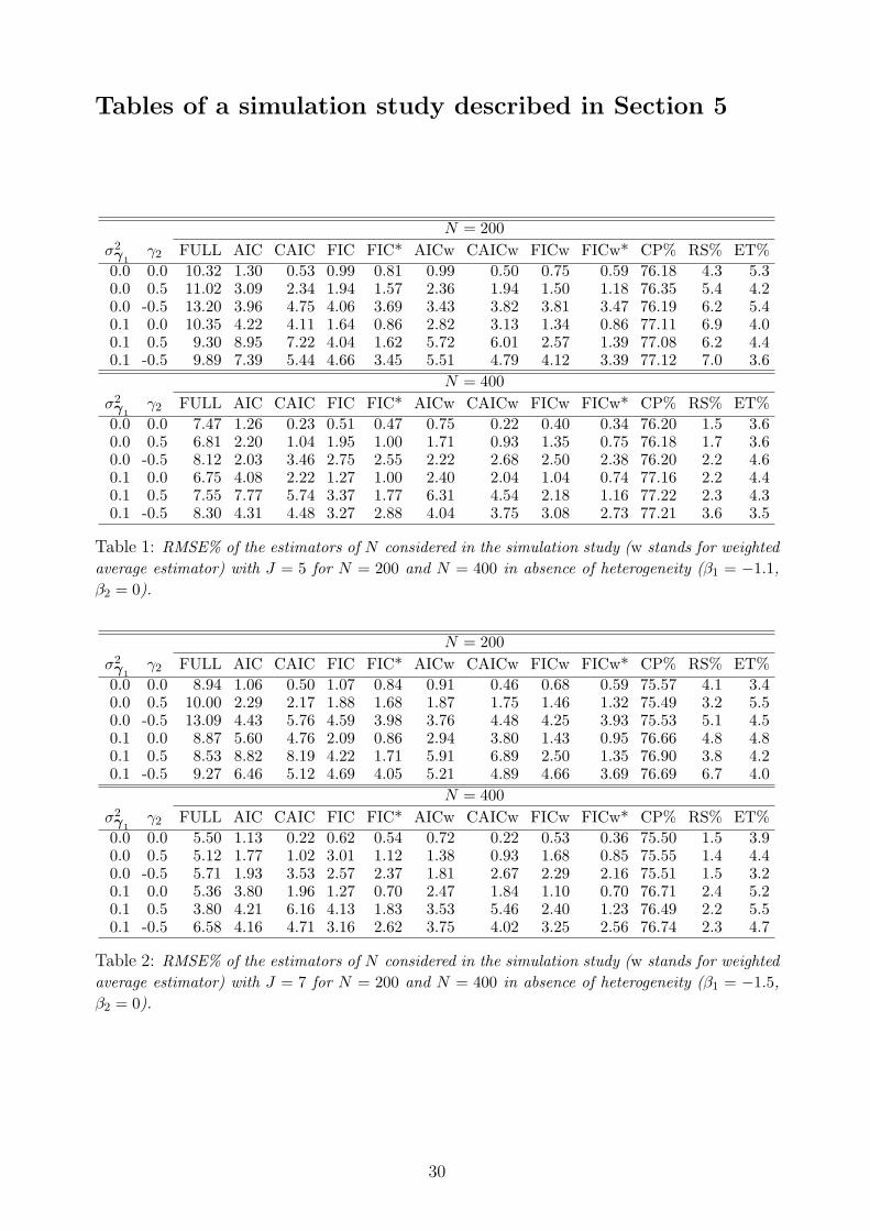
Tables of a simulation study described in Section 5

N = 200σ2γ1

γ2 FULL AIC CAIC FIC FIC* AICw CAICw FICw FICw* CP% RS% ET%0.0 0.0 10.32 1.30 0.53 0.99 0.81 0.99 0.50 0.75 0.59 76.18 4.3 5.30.0 0.5 11.02 3.09 2.34 1.94 1.57 2.36 1.94 1.50 1.18 76.35 5.4 4.20.0 -0.5 13.20 3.96 4.75 4.06 3.69 3.43 3.82 3.81 3.47 76.19 6.2 5.40.1 0.0 10.35 4.22 4.11 1.64 0.86 2.82 3.13 1.34 0.86 77.11 6.9 4.00.1 0.5 9.30 8.95 7.22 4.04 1.62 5.72 6.01 2.57 1.39 77.08 6.2 4.40.1 -0.5 9.89 7.39 5.44 4.66 3.45 5.51 4.79 4.12 3.39 77.12 7.0 3.6

N = 400σ2γ1


Table 1: RMSE% of the estimators of N considered in the simulation study (w stands for weightedaverage estimator) with J = 5 for N = 200 and N = 400 in absence of heterogeneity (β1 = −1.1,β2 = 0).

N = 200σ2γ1


N = 400σ2γ1


Table 2: RMSE% of the estimators of N considered in the simulation study (w stands for weightedaverage estimator) with J = 7 for N = 200 and N = 400 in absence of heterogeneity (β1 = −1.5,β2 = 0).

30

N = 200σ2γ1


N = 400σ2γ1


Table 3: RMSE% of the estimators of N considered in the simulation study (w stands for weightedaverage estimator) with J = 5 for N = 200 and N = 400 in the presence of heterogeneity (β1 =−1.1, β1 = 0.5).

N = 200σ2γ1


N = 400σ2γ1


Table 4: RMSE% of the estimators of N considered in the simulation study (w stands for weightedaverage estimator) with J = 7 for N = 200 and N = 400 in presence of heterogeneity (β1 = −1.5,β2 = 0.5).

31

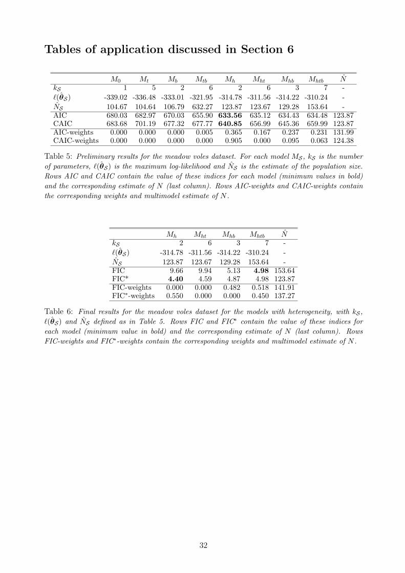
Tables of application discussed in Section 6

M0 Mt Mb Mtb Mh Mht Mhb Mhtb NkS 1 5 2 6 2 6 3 7 -`(θS) -339.02 -336.48 -333.01 -321.95 -314.78 -311.56 -314.22 -310.24 -NS 104.67 104.64 106.79 632.27 123.87 123.67 129.28 153.64 -AIC 680.03 682.97 670.03 655.90 633.56 635.12 634.43 634.48 123.87CAIC 683.68 701.19 677.32 677.77 640.85 656.99 645.36 659.99 123.87AIC-weights 0.000 0.000 0.000 0.005 0.365 0.167 0.237 0.231 131.99CAIC-weights 0.000 0.000 0.000 0.000 0.905 0.000 0.095 0.063 124.38

Table 5: Preliminary results for the meadow voles dataset. For each model MS , kS is the numberof parameters, `(θS) is the maximum log-likelihood and NS is the estimate of the population size.Rows AIC and CAIC contain the value of these indices for each model (minimum values in bold)and the corresponding estimate of N (last column). Rows AIC-weights and CAIC-weights containthe corresponding weights and multimodel estimate of N .

Mh Mht Mhb Mhtb NkS 2 6 3 7 -`(θS) -314.78 -311.56 -314.22 -310.24 -NS 123.87 123.67 129.28 153.64 -FIC 9.66 9.94 5.13 4.98 153.64FIC* 4.40 4.59 4.87 4.98 123.87FIC-weights 0.000 0.000 0.482 0.518 141.91FIC∗-weights 0.550 0.000 0.000 0.450 137.27

Table 6: Final results for the meadow voles dataset for the models with heterogeneity, with kS ,`(θS) and NS defined as in Table 5. Rows FIC and FIC∗ contain the value of these indices foreach model (minimum value in bold) and the corresponding estimate of N (last column). RowsFIC-weights and FIC∗-weights contain the corresponding weights and multimodel estimate of N .

32

Documents

Focused information criterion for capture-recapture models for closed populations (short title: FIC for closed capture-recapture models)