Continuous-time spatially explicit capture–recapturemodels, with an application to a jaguar camera-trap

survey

DavidBorchers1, GregDistiller2*, Rebecca Foster3, 4, Bart Harmsen3, 4 and LorenzoMilazzo5

1School ofMathematics and Statistics, Centre for Research into Ecological and Environmental Modelling, TheObservatory,

BuchananGardens, University of St Andrews, Fife KY16 9LZ, UK; 2Statistics in Ecology, Environment andConservation

(SEEC), Department of Statistical Sciences, University of Cape Town, Private BagX3, Rondebosch 7701, South Africa;3Panthera, 8West 40th Street, 18th Floor, NewYork, NY 10018, USA; 4Environmental Research Institute (ERI), University of

Belize, POBox 340Belmopan, Belize; and 5Cambridge Infectious Diseases (CID), University of Cambridge,Madingley Road,

Cambridge CB3 0ES,UK

Summary

1. Many capture–recapture surveys of wildlife populations operate in continuous time, but detections are typi-

cally aggregated into occasions for analysis, evenwhen exact detection times are available. This discards informa-

tion and introduces subjectivity, in the form of decisions about occasion definition.

2. We develop a spatiotemporal Poisson process model for spatially explicit capture–recapture (SECR) surveys

that operate continuously and record exact detection times.We show that, except in some special cases (including

the case in which detection probability does not change within occasion), temporally aggregated data do not pro-

vide sufficient statistics for density and related parameters, and that when detection probability is constant over

time, our continuous-time (CT) model is equivalent to an existing model based on detection frequencies. We use

themodel to estimate jaguar density from a camera-trap survey and conduct a simulation study to investigate the

properties of a CT estimator and discrete-occasion estimators with various levels of temporal aggregation. This

includes investigation of the effect on the estimators of spatiotemporal correlation induced by animal movement.

3. TheCT estimator is found to be unbiased andmore precise than discrete-occasion estimators based on binary

capture data (rather than detection frequencies) when there is no spatiotemporal correlation. It is also found to

be only slightly biased when there is correlation induced by animal movement, and to be more robust to inade-

quate detector spacing, while discrete-occasion estimators with binary data can be sensitive to occasion length,

particularly in the presence of inadequate detector spacing.

4. Our model includes as a special case a discrete-occasion estimator based on detection frequencies, and at the

same time lays a foundation for the development of more sophisticated CT models and estimators. It allows

modelling within-occasion changes in detectability, readily accommodates variation in detector effort, removes

subjectivity associated with user-defined occasions and fully utilizes CT data. We identify a need for developing

CT methods that incorporate spatiotemporal dependence in detections and see potential for CT models being

combined with telemetry-based animalmovementmodels to provide a richer inference framework.

Key-words: animal movement, data aggregation, density estimation, statistical methods,

sufficiency

Introduction

Monitoring elusive species such as forest-dwelling carnivores

that occur at low densities and range over wide areas is diffi-

cult, as is monitoring species that are difficult to trap or detect

visually, but many such species are of high conservation con-

cern. The estimation of density and detectability are common

in population monitoring and are crucial parameters for elu-

sive species (Stuart et al. 2004, Thompson 2004).

Technological advances in non-invasive sampling methods

such as scat or hair collection for genetic analysis, camera-trap-

ping and acoustic detection have led to newways of ’capturing’

individuals, that are particularly useful for species that are diffi-

cult to survey using more conventional methods. Camera-trap

arrays in particular have become an important tool for assess-

ment and management of species that are hard to detect by

other means. They have been used with capture–recapture

(CR) methods for various species that are individually identifi-

able from photographs, including felids, canids, ursids, hyae-

nids, procynoids, tapirids and dasypodids (see references in*Correspondence author. E-mail: Greg.Distiller@uct.ac.za

© 2014 The Authors. Methods in Ecology and Evolution © 2014 British Ecological Society

Methods in Ecology and Evolution 2014 doi: 10.1111/2041-210X.12196

Foster & Harmsen 2012), and are increasingly used with

spatially explicit capture–recapture (SECR) methods. SECR

incorporates spatial information on capture locations and

allows inferences to be drawn about the underlying process

governing the locations of individuals, as well as providing esti-

mates of density without the need for separate estimates of the

effective sampling area (Efford 2004, Borchers & Efford 2008,

Efford, Borchers &Byrom 2009a, Royle et al. 2009).

When a CR study (conventional or SECR) involves physi-

cally capturing individuals, the survey process generates

well-defined sampling occasions. But, when there is no physical

capture and release, as in the case of camera-trap studies or

acoustic CR surveys that record times of detection, there is no

well-defined sampling occasion. In such cases, aggregating data

into capture occasions introduces subjectivity (the occasion

length chosen by the analyst) and discards some information

(the exact times of capture). Continuous-time (CT) models

avoid these problems. The earliest CT model is probably that

of Craig (1953). It assumed equal catchability for all individuals

at all times, but has since been extended to allow individual het-

erogeneity (Boyce et al. 2001). Most CT estimators use martin-

gale estimating functions (Becker 1984; Yip 1989; Becker &

Heyde 1990; Yip, Huggins & Lin 1995; Lin & Yip 1999; Yip

et al. 1999; Hwang & Chao 2002; Yip &Wang 2002), although

Nayak (1988), Becker & Heyde (1990) and Hwang, Chao &

Yip (2002) developed maximum likelihood estimators (MLEs)

and Chao & Lee (1993) developed a CT estimator based on

sample coverage. Of the CT models in the literature, only the

models of Nayak (1988), Yip (1989) and Hwang, Chao & Yip

(2002) estimate detectability and abundance simultaneously, in

common with the estimator we develop below.

There is no consensus on the utility of CT estimators. Some

authors concluded that the use of a discrete-occasion model to

analyse a CT data set will bias estimates (Yip & Wang 2002;

Barbour, Ponciano & Lorenzen 2013), while others found no

benefit over discrete-occasion estimators (e.g. Chao & Lee

1993;Wilson&Anderson 1995).We show inAppendix S3 that

Chao&Lee’s (1993) conclusion that capture times are uninfor-

mative about abundance does not hold in general. We develop

CTSECR likelihoods andMLEswhich, unlike any existingCT

models, are parameterised in termsof populationdensity rather

than abundance, and crucially, incorporate a model for (unob-

served) individual activity centres. An activity centre is the cen-

tre of gravity of an individual’s locations over the duration of

the survey. It may have biological interpretation, for example

as a home range centre, but need not. Ourmodel is obtained by

formulating the SECR survey process as a non-homogeneous

spatiotemporal Poisson process, in which events are detections

at points in space and time (see Cook & Lawless 2007, for a

comprehensive overview of recurrent event processes, of which

Poisson processes are a special case). We note that the interac-

tion between recurrent event processes and CR methods was

identified by Chao & Huggins (2005), p. 85) as ’a fruitful area

for future research’,whichwe explore in this paper.

We focus on the development of SECR methods for data

from camera-trap surveys, but ourmodels are also appropriate

for any CR survey with continuous sampling in which capture

times are recorded. This includes acoustic SECR surveys such

as those described in Efford, Dawson & Borchers (2009b),

Dawson & Efford (2009) or Borchers et al. (2013), although

recapture identification may be difficult in such surveys. CT

SECR models also provide the basis for varying-effort SECR

methods such as those of Efford, Borchers andMowat (2013),

and we show how discrete-occasion models arise from a CT

formulation.

We assume independence between captures, conditional on

activity centre location. This is almost certainly violated to

some degree in camera-trap studies because individuals are

only detected when they move within range of a camera, and

an individual’s locations are temporally correlated.We investi-

gate sensitivity to violation of this assumption.

We develop a general CT SECR likelihood and then evalu-

atemodels under the assumptions of constant detection proba-

bility over time and constant intensity of the spatial point

process governing the number and locations of activity centres.

In this case, the CT likelihood is equivalent to a single-occasion

Poisson count likelihood spanning the whole survey, in which

the data are the capture frequencies of each individual at each

detector (see Appendix S3). Simulations are used to compare

the CT estimator for this case with discrete-occasion estimators

based on binary data within occasions and detectors (i.e. in

which, each individual’s capture frequency at each detector

within an occasion is reduced to a binary indicator of detection

or not). We compare various levels of temporal aggregation

both when the assumption of independence holds and when it

is violated by simulating correlated animalmovement.

Materials andmethods

STUDY SITE AND CAMERA TRAPPING OF JAGUARS

Jaguars (Panthera onca) are near threatened and their global popula-

tion is declining (Caso et al. 2008), and population monitoring is diffi-

cult because they occur at low densities, range widely and are elusive,

often inhabiting thick habitat. Over the past decade, the challenge of

detecting jaguars for population estimation has been facilitated by cam-

era traps, following the work of Silver et al. 2004; however, reliable and

robust density estimates of jaguars are rarely obtained (see Foster &

Harmsen 2012; Tobler & Powell 2013).

We estimate male jaguar density in the Cockscomb Basin Wildlife

Sanctuary inBelize fromcamera-trap data. The sanctuary encompasses

490 km2 of secondary tropical moist broadleaf forest at various stages

of regeneration following anthropogenic and natural disturbance (for

more details, see Harmsen et al. 2010b). To the west, the sanctuary

forms a contiguous forest block with the protected forests of the Maya

Mountain Massif ( 5000 km2 of forest). To the east, the sanctuary is

partially buffered by unprotected forest beyond which is a mosaic of

pine savannah, shrub landandbroadleaf forest, inter-dispersedwith vil-

lages and farms. Jaguars are found throughout this landscape (Foster,

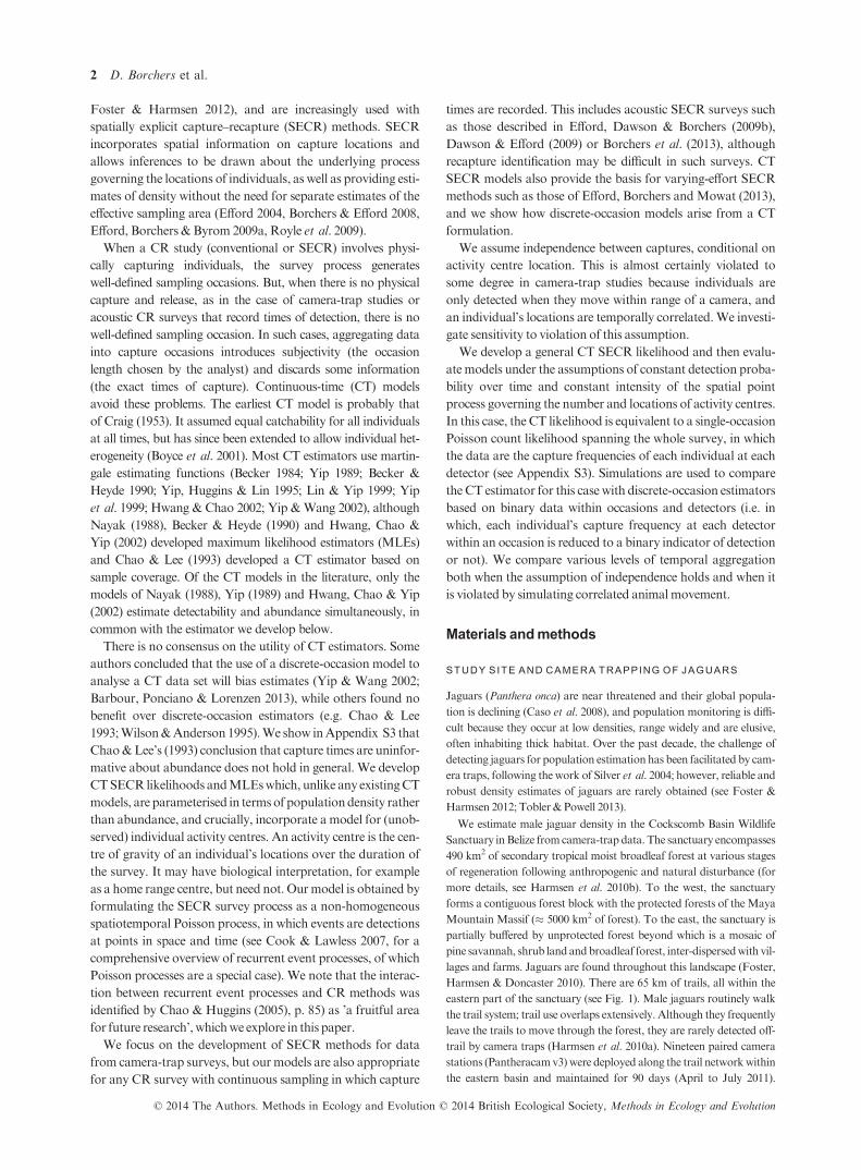
Harmsen & Doncaster 2010). There are 65 km of trails, all within the

eastern part of the sanctuary (see Fig. 1). Male jaguars routinely walk

the trail system; trail use overlaps extensively. Although they frequently

leave the trails to move through the forest, they are rarely detected off-

trail by camera traps (Harmsen et al. 2010a). Nineteen paired camera

stations (Pantheracamv3)were deployed along the trail networkwithin

the eastern basin and maintained for 90 days (April to July 2011).

© 2014 The Authors. Methods in Ecology and Evolution © 2014 British Ecological Society, Methods in Ecology and Evolution

2 D. Borchers et al.

Neighbouring stations had an average spacingof 20km (11 to 31 km).

The cameras used have an enforced 8 s delay between consecutive pho-

tos, anddigital photographic dataweredownloaded every 2weeks.

CONTINUOUS-T IME MODELS FOR PROXIMITY

DETECTORS

We refer to both capture and detection as ‘detection’, and to all detec-

tors, including traps, as ‘detectors’.

We model the process generating detections as a non-homogeneous

Poissonprocess (NHPP) inspaceandtime, inwhich theeventsaredetec-

tions. This model is governed by a hazard of detection, which can vary

with location and timeand is equal to the expectednumber of detections

per unit time at the location and time. The model allows this hazard to

change with location (to accommodate lower capture probability for

individuals with activity centres farther from detectors, for example),

time (to accommodate different animal activity levels at different times

of day, for example) andother explanatory variables, butwe assume ini-

tially that the hazard for any individual at any time is independent of the

individual’s capture history up to that time. We develop a model and

estimator under this assumption and then investigate its performance

when the hazard of detection does depend onwhere andwhen individu-

als were previously detected (as a consequence of correlated animal

movement). Parameters and standard errors were estimated using a

Newton-typealgorithmwith functionnlm inR (RCoreTeam,2013).

Continuous-time proximity detector likelihood

We consider a survey in which we have an array of K continuously

samplingproximitydetectors.Thekeydifference between the likelihood

presented here and adiscrete-occasion SECR likelihood is that there are

no longer occasions, but instead, a continuous survey running for a per-

iod (0,T). Instead of a capture history of length S (if there were S occa-

sions) for the ith individual at detector k, we have xik captures of the

individual at detector k at times tik ¼ ðtik1; . . .; tikxikÞ. For brevity, we

let t = tik (i = 1,. . .,n;k = 1,. . .,K) denote the set of all detection times.

To simplify presentation of the likelihood, we start by considering a

single individual (the ith individual), with activity centre at xi, and a sin-

gle detector (the kth detector). By considering tik to be a realization of

an NHPP in time, we obtain an expression for the probability density

function (pdf) of tik. This is analogous to the probability of obtaining a

capture history at detector k for individual i in a discrete-occasion for-

mulation, but it is worth noting that both the length of tik (i.e. xik) and

the times that it contains are random variables, whereas for a discrete-

occasion survey, the length of a capture history is fixed by the number

of occasions used.

Using the pdf of tik, we obtain an expression for the probability of

detecting individual i at all. Then, following Borchers & Efford (2008),

we assume that the (unobserved) activity centres of detected individuals

are realizations of a filtered spatial NHPP, with filter at a location x

being the detection probability at that location. This gives rise to a joint

probability model for the number of individuals detected (n) and their

detection times at detectors (t). When considered as a function of the

unknownmodel parameters, this is the CT SECR likelihood function.

The pdf of tik. In a CT formulation, the discrete-occasion expression

for the probability of detecting individual i at detector k on an occasion

is replaced by a detection hazard function that specifies the expected

detection rate per unit time at detector k of an individual, at time t,

given the location of its activity centre (xi for individual i). This hazard

function hk(t,xi;h) depends on the distance from detector k to the indi-

vidual’s activity centre (xi), and we make this explicit when we specify

models for hk(t,xi;h), but for notational, brevity we do not make the

dependence on distance explicit otherwise. The hazard function has an

unknown vector of detection function parameters h. The ‘survivor

function’ for individual i at detector k over thewhole survey (the proba-

bility of individual i not being detected on the detector by time T) is

SkðT;xi; hÞ ¼ exp R T0 hkðu;xi; hÞ du

and hence 1Sk(T,xi;h) is

the probability of detection in (0,T).

In a similar vein, the link between a CT detection hazard and a dis-

crete-occasion detection probability, pks(xi;h) for detector k on occasions, of length Ts = tsts1 (running from ts1 to ts) is: pksðxi; hÞ ¼ 1exp R tsts1

hksðt; xi; hÞ du. Under the assumption of a constant haz-

ard, solving this for hks(t,xi;h) leads to a hazardwith the following form:

hksðxi; hÞ ¼ log 1 pksðxi; hÞf g=Ts eqn 1

In our analyses, we use hazard functions in which pks(xi;h) for a spec-ified occasion length has a half-normal form: pksðxi; hÞ ¼ g0;Ts

expfdkðxiÞ2=ð2r2Þg, where dk(xi) is the distance from xi to detector k, and

g0;Tsand r are parameters to be estimated. The parameter g0;Ts

is the

probability that an individual with activity centre located at a detector

is detected in a time period of length Ts, while r is the scale parameter

of the half-normal detection function, and determines the range over

which an individual is detectable.

Assuming that, conditional on the activity centre location, the times

of detections are independent, we can model the number of detections,

xik, and the detection times tik as a nonhomogeneous Poisson process

with pdf as follows [see Cook&Lawless 2007, Theorem 21 on page 30,and Equation (213) on page 32]:

fkðtikjxi; hÞ ¼ SkðT;xi; hÞYxik

r¼1

hkðtikr;xi; hÞ eqn 2

(We omitxik from the LHS for brevity, because given tik,xik is known.)

For those familiar with the definition of hazard functions in terms of

the pdf and survivor function, we note that hk(tikr,xi;h) = fk(tikr|xi;h)/Sk((tikrtik(r1)),xi;h).

Equation (2) is a generalization of the expression obtained by

Hwang et al. (2000, p. 43) for their modelMt (given by their expression

for Li), and of the expression of Chao & Huggins (2005, p. 80) for the

case in which hk(tikr,xi;h) is constant. Both sets of authors use k for the

hazard, whereas we use h(). In addition to locating these models in the

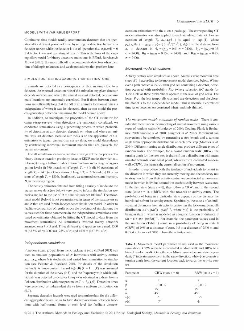
Fig. 1. Camera-trap locations within Cockscomb Basin Wildlife

Sanctuary, Belize.

© 2014 The Authors. Methods in Ecology and Evolution © 2014 British Ecological Society, Methods in Ecology and Evolution

Continuous-time SECR 3

Poisson process literature, our generalization involves the inclusion of

x as a latent variable (see below), and extension tomultiple detectors.

Multiple detectors and individuals. An individual’s overall detec-

tion frequency across the K detectors is denoted xi ¼PK

k¼ 1 xik, and

the event xi>0 indicates detection by some detector. The combined

detection hazard over all detectors at time t is hðt; xi; hÞ ¼ PKk¼ 1

hkðt;xi; hÞ, and the overall probability of detection in (0,T) over all

detectors is p(xi;h) = p(xi>0|xi;h) = 1S(T,xi;h), where SðT; xi; hÞ¼ exp R T0 hðt;xi; hÞ

is the overall survivor function.

Following Borchers & Efford (2008), we assume that activity cen-

tres occur independently in the plane according to an NHPP with

intensity D(x;/) at x, where x is any point in the survey region and

/ is a vector of unknown parameters that govern the intensity and

hence the distribution of activity centres. D(x;/) is the expected

activity centre density at x. Activity centres are assumed not to move

during the survey.

The likelihood for / and h is the joint distribution of the number of

animals captured n, and the density of the outcome ‘xik events, at times

tik1\. . .\tikxrmikr’, for all i and k. This can be written in terms of the

marginal distribution of n and the conditional distribution of t given n.

Lðh;/ j n; tÞ ¼ Pðn j /; hÞftðtjn; h;/Þ eqn 3

If individuals are detected independently, n is a Poisson random

variable with parameter k(h,/) = ∫AD(x;/)p(x;h) dx, where p(x;h) isthe probability of an individual with activity centre at x being detected

at all and the integral is over all points x in the area A in which activity

centres occur.

We obtain an expression for ft(t|n,h,/) in Appendix S1 and show

that, given the detection times of all detected individuals, t, the likeli-

hood for/ and h is

Lð/; hjn; tÞ ¼ expkð/;hÞ

n!

Yni¼1

ZA

Dðxi;/ÞSðT;xi; hÞ

YKk¼1

Yxik

r¼1

hkðtikr;xi; hÞ dxeqn 4

The integral is over all possible activity centre locations that could

have led to a detection on the survey. (See section 42 of Borchers & Ef-

ford 2008, for a brief discussion of this issue.)

It is sometimes useful to write this likelihood in terms of themarginal

distribution of xik and the conditional distribution of tik given xik. The

capture frequency over the survey for individual i at detector k has a

Poisson distribution with parameterHkðxi; hÞ ¼ R T0 hkðt;xi; hÞ dt [see

Cook&Lawless 2007, Equation (215) on page 32]:

Pkðxikjxi; hÞ ¼ Hkðxi; hÞxik expHkðxi ;hÞ

xik!¼ Hkðxi; hÞxikSkðT;xi; hÞ

xik!

eqn 5

It follows from this and eqn (2) that the conditional pdf of detection

times tik, givenxik, for the ith animal is

ftjx;kðtikjxik;xi; hÞ ¼ xik!Yxik

r¼1

hkðtikrjxi; hÞHkðxi; hÞ eqn 6

and hence that

Lð/; hjn; tÞ ¼ ekðh;/Þ

n!

Yni¼1

ZA

Dðxi;/ÞYKk¼1

Pkðxikjxi; hÞ

Yxik

r¼1

ftjx;kðtikjxik; xi; hÞ dxeqn 7

Constant density, constant hazard likelihood

One simple special case arises when density is uniform, that is the spa-

tial Poisson process governing activity centre locations is homoge-

neous, and the detection hazards do not change with time. In this case,

D(x;/) is a constant (D), k(h,/) = Da(h) (where a(h) = ∫Ap(x;h) dx is

the effective survey area), hk(t,xi;h) = hk(xi;h) and soHk(xi;h) = Thk(xi;

h). As a result, eqn (6) becomes ftjx;kðtikjxik;xi; hÞ ¼ xik!Qxik

r¼ 1 T1

and the likelihood eqn (7) simplifies to

LðD; hjn; tÞ ¼ DneDaðhÞ

n!

Yni¼1

ZA

YKk¼1

Pkðxikjxi; hÞ dx !

Yni¼1

YKk¼1

xik!Yxik

r¼1

1

T

! eqn 8

The second term in large brackets is the pdf of the detection times t,

given the detection frequencies xik (i = 1,. . .,n;k = 1,. . .,K). Because

this term does not contain any model parameters, and the term in

the first large brackets contains the parameters and the detection

frequencies xik but not the detection times, it follows (from the

Fisher–Neyman Factorization Theorem for sufficiency) that in this

case, the detection frequencies are sufficient statistics for the parame-

ters h andD, that is, that no information about D is lost by discarding

the detection times. Chao & Lee (1993) obtained this result for the

case with a single detector, no x, and a model parameterised in terms

of abundance N rather than density D – but the result does not hold

in general, as we discuss below.

Relationship to Poisson countmodels

One can see from eqn (8) that under the above assumptions, the CT

model gives rise to a Poisson count model, as Pk(xik) is a Poisson prob-

abilitymass function (pmf) with rate parameterTshks(xi;h) and the termin the second large bracket can be neglected because it is constant with

respect to the parameters. This model was proposed in Appendix S1 of

Efford,Dawson&Borchers (2009b), and a similarmodelwas proposed

by Royle et al. (2009). The CTmodel provides an interpretation of the

Poisson rate parameter of these models as the cumulative detection

hazard,Tshks(xi;h). BothEfford,Dawson&Borchers (2009b) andRoy-

le et al. (2009) proposedmodellingTshks(xi;h) using the same functional

forms as are used for the probability of detecting an individual within

an occasion, but allowing an intercept greater than 1. This may be a

reasonable strategy, but modellers should be aware that pks(xi;h) andhks(xi;h) necessarily have different shapes because pks(xi;h) = 1exp Tshks(xi;h). So for example, assuming a half-normal shape for

the Poisson rate parameter (as do Royle et al. 2009), Tshks(xi;

h) = k0expdk(xi)2/r2 generates a shape for the detection function

pks(xi);h) that is not half-normal.

Lack of sufficiency of detection frequencies

In Appendix S3, we show that the discrete-occasion Bernoulli, bino-

mial and Poisson models are reduced-data versions of the CT model

and that the detection histories or detection frequencies Ω = xiks

(i = 1,. . .,n;k = 1,. . .,K;s = 1,. . .,S, where S is the number of occasions

in the survey) are not in general sufficient statistics for h and /, that isthat in general detection time is informative. A notable exception is

when the detection hazard is constant within occasions. In this case,

discarding detection times does not discard information about popula-

tion density. Reducing counts to a binary event does however discard

information, and the consequences of this reduction are explored in the

first simulation below.

© 2014 The Authors. Methods in Ecology and Evolution © 2014 British Ecological Society, Methods in Ecology and Evolution

4 D. Borchers et al.

MODELS WITH VARIABLE EFFORT

Continuous-time models readily accommodate detectors that are oper-

ational for different periods of time, by setting the detection hazard at a

detector to zero while the detector is out of operation (i.e. hk(t,x;h) = 0

if detector k was not operating at time t). This is the basis of the vary-

ing-effort model for binary detectors and counts in Efford, Borchers &

Mowat (2013). It is more difficult to accommodate detectors when their

time of failing is unknown, andwe do not address that problem here.

SIMULATION TESTING CAMERA-TRAP ESTIMATORS

If animals are detected as a consequence of their moving close to a

detector, the expected detection rate of the animal at any given detector

depends on when and where the animal was last detected, because ani-

mals’ locations are temporally correlated. But if times between detec-

tions are sufficiently long that the pdf of an animal’s location at time t is

independent of where it was last detected, then we can model the pro-

cess generating detection times using themodel derived above.

In addition, to investigate the properties of the CT estimator for

camera-trap surveys when detections are temporally correlated, we

conducted simulations using a generating process in which probabil-

ity of detection at any detector depends on when and where an ani-

mal was last detected. Because our focus is on the application of CT

estimators to jaguar camera-trap survey data, we model dependence

by constructing individual movement models that are plausible for

jaguar movement.

For all simulation scenarios, we also investigated the properties of a

binary discrete-occasion proximity detector SECRmodel (in whichxiks

is binary) using a half-normal detection function and a range of aggre-

gation levels: (i) 360 occasions of length Ts = 6 h (ii) 90 occasions of

length Ts = 24 h (iii) 30 occasions of length Ts = 72 h and (iv) 18 occa-

sions of length Ts = 120 h. In all cases, we assumed constant intensity,

D, in the survey region.

The density estimates obtained from fitting a variety ofmodels to the

jaguar survey data (see below) were used to inform the simulation sce-

narios and led to the use of D = 4 individuals per 100 km2. The move-

ment model (below) is not parameterised in terms of the parameters g0andr that are used for the independence simulationmodel. In order to

facilitate comparison of results across the two kinds of simulations, the

values used for these parameters in the independence simulations were

based on estimates obtained by fitting the CT model to data from the

movement simulations. All simulations involved twenty detectors

arranged on a 49 5 grid. Three different grid spacings were used: 1500

m (625%ofr), 3000m (125%ofr) and 4500m (1875%ofr).

Independence simulations

Functionsim.popn from the R packagesecr (Efford 2013) was

used to simulate populations of N individuals with activity centres

x1,. . .,xN, where N is stochastic and varied from simulation to simula-

tion (see Fewster & Buckland 2004, for details of the simulation

method). A time-constant hazard hk(xi;h) (k = 1,. . .,K) was assumed

for the duration of the survey (0,T), and the frequency with which indi-

vidual iwas detected by detector k (xik) was obtained as a draw from a

Poisson distribution with rate parameter T 9 hk(xi;h). Detection times

were generated by independent draws from a uniform distribution on

(0,T).

Separate detection hazards were used to simulate data for the differ-

ent aggregation levels, so as to have discrete-occasion detection func-

tions with half-normal forms at each level (to facilitate discrete-

occasion estimation with the secr package). The corresponding CT

model estimator was also applied to each simulated data set. For an

occasion of length Ts, hksðxi; hTsÞ is equal to eqn (1), where

pksðxi; hTsÞ ¼ g0;Ts

expfdkðxiÞ2=ð2r2Þg, dk(xi) is the distance from

xi to detector k, h6 = (g0,6 = 001,r = 2400), h24 = (g0,24=005,r = 2400), h72 = (g0,72 = 015,r = 2400) and h120 = (g0,120 = 025,r = 2400).

Movementmodel simulations

Activity centres were simulated as above. Animals were moved in time

steps of 1 h according to the movement model described below.When-

ever a path crossed a 2509250 m grid cell containing a detector, detec-

tion occurred with probability PGC (where subscript GC stands for

’Grid Cell’ as these probabilities operate at the level of grid cells). The

lower PGC, the less temporally clustered are detections and the closer

the model is to the independence model. This is because a correlated

time series becomes less correlated when randomly thinned.

The movement model: a mixture of random walks. There is con-

siderable literature on themodelling of animal movement using various

types of random walks (Morales et al. 2004; Codling, Plank & Benha-

mou 2008; Smouse et al. 2010; Langrock et al. 2012). Movement can

conveniently be simulated by generating a step length and a turning

angle from appropriate distributions at each time step (Morales et al.

2004). Different turning angle distributions produce different types of

random walks. For example, for a biased random walk (BRW), the

turning angle for the next step is drawn from a distribution with mean

oriented towards some focal point, whereas for a correlated random

walk (CRW), themean is the current direction ofmovement.

In order to reproduce both the tendency of individuals to persist in

the direction in which they are currently moving and the tendency not

to stray too far from their activity centre, we constructed a movement

model in which individuals transition stochastically between two states.

In the first state (state s = 0), they follow a CRW, and in the second

state (state s = 1), a BRW with bias towards an activity centre. The

probability of being in a particular state depends on the distance the

individual is from its activity centre. Specifically, the state s of an indi-

vidual at distance d from its activity centre has the following Bernoulli

distribution s|d c(d)s(1c(d))1s, where c(d) is the probability of

being in state 1, which is modelled as a logistic function of distance: c(d) = (1+ exp a+bd)1. For example, the parameter values used in

the simulation (Table 1) result in a probability of being in state 0

(CRW) of 095 at a distance of zero, 05 at a distance of 2500 m and

005 at a distance of 5000m from the activity centre.

Table 1. Movement model parameter values used in the movement

simulations. CRW refers to a correlated random walk and BRW to a

biased random walk. Only the von Mises parameters are state depen-

dent; 0o indicates movement in the same direction, while/t represents a

turning angle from the current location back towards the activity cen-

tre

Parameter CRW (state s = 0) BRW (state s = 1)

a 3 3

b 00012 00012a 750 750

b 450 450

j(s) 6 05l(s) 0o /t

© 2014 The Authors. Methods in Ecology and Evolution © 2014 British Ecological Society, Methods in Ecology and Evolution

Continuous-time SECR 5

The size of each movement step (l) is a draw from a gamma distribu-

tion with mean step length a and standard deviation b: lGamma(a2/

b2,b2/a). The turning angle (/), given that the individual is in state s, is

drawn from a von Mises distribution /|s von Mises(l(s),j(s)) wherel(s) is the mean and j(s) the concentration parameter. Values for j(s)close to zero generate something close to a uniform distribution on the

circle, whereas larger values will place increasingmass around themean

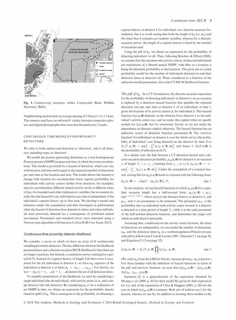
value. Table 1 shows the movement model parameter values used in

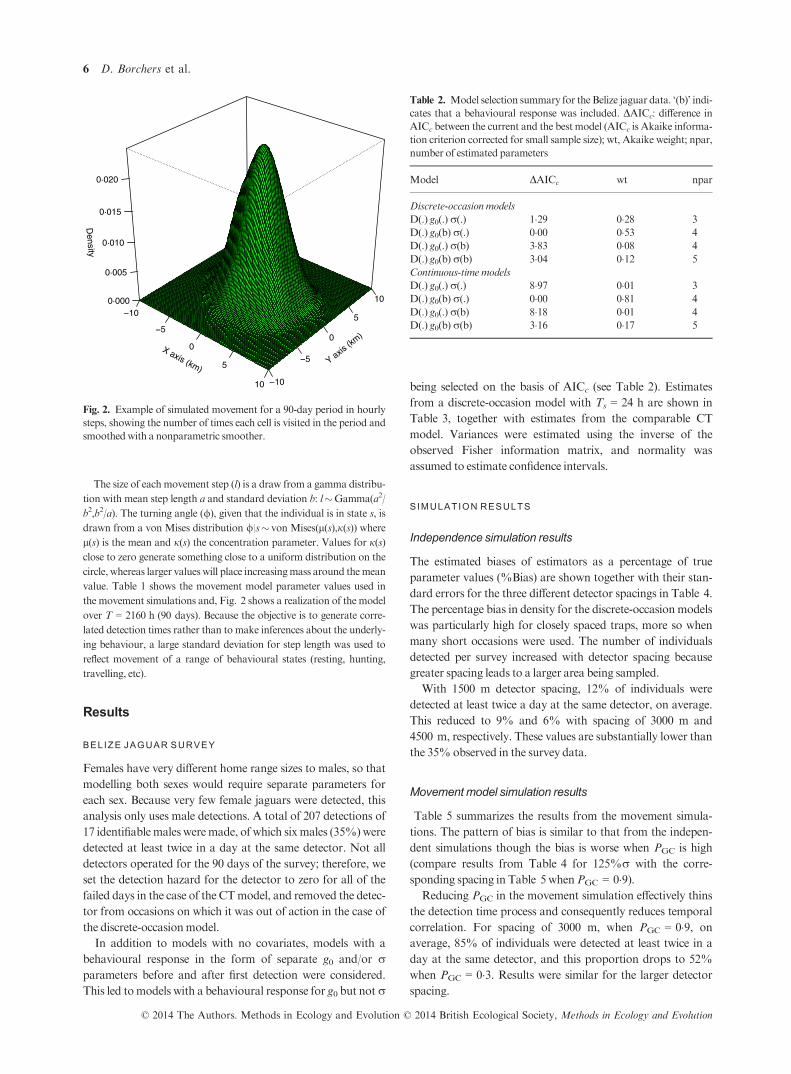
the movement simulations and, Fig. 2 shows a realization of the model

over T = 2160 h (90 days). Because the objective is to generate corre-

lated detection times rather than to make inferences about the underly-

ing behaviour, a large standard deviation for step length was used to

reflect movement of a range of behavioural states (resting, hunting,

travelling, etc).

Results

BELIZE JAGUAR SURVEY

Females have very different home range sizes to males, so that

modelling both sexes would require separate parameters for

each sex. Because very few female jaguars were detected, this

analysis only uses male detections. A total of 207 detections of

17 identifiablemales weremade, of which sixmales (35%)were

detected at least twice in a day at the same detector. Not all

detectors operated for the 90 days of the survey; therefore, we

set the detection hazard for the detector to zero for all of the

failed days in the case of the CTmodel, and removed the detec-

tor from occasions on which it was out of action in the case of

the discrete-occasionmodel.

In addition to models with no covariates, models with a

behavioural response in the form of separate g0 and/or rparameters before and after first detection were considered.

This led tomodels with a behavioural response for g0 but notr

being selected on the basis of AICc (see Table 2). Estimates

from a discrete-occasion model with Ts = 24 h are shown in

Table 3, together with estimates from the comparable CT

model. Variances were estimated using the inverse of the

observed Fisher information matrix, and normality was

assumed to estimate confidence intervals.

SIMULATION RESULTS

Independence simulation results

The estimated biases of estimators as a percentage of true

parameter values (%Bias) are shown together with their stan-

dard errors for the three different detector spacings in Table 4.

The percentage bias in density for the discrete-occasionmodels

was particularly high for closely spaced traps, more so when

many short occasions were used. The number of individuals

detected per survey increased with detector spacing because

greater spacing leads to a larger area being sampled.

With 1500 m detector spacing, 12% of individuals were

detected at least twice a day at the same detector, on average.

This reduced to 9% and 6% with spacing of 3000 m and

4500 m, respectively. These values are substantially lower than

the 35%observed in the survey data.

Movementmodel simulation results

Table 5 summarizes the results from the movement simula-

tions. The pattern of bias is similar to that from the indepen-

dent simulations though the bias is worse when PGC is high

(compare results from Table 4 for 125%r with the corre-

sponding spacing in Table 5 whenPGC = 09).Reducing PGC in the movement simulation effectively thins

the detection time process and consequently reduces temporal

correlation. For spacing of 3000 m, when PGC = 09, on

average, 85% of individuals were detected at least twice in a

day at the same detector, and this proportion drops to 52%

when PGC = 03. Results were similar for the larger detector

spacing.

X axis (km)

−10

−5

0

5

10

Y axis (k

m)

−10

−5

0

5

10

Density

0·000

0·005

0·010

0·015

0·020

Fig. 2. Example of simulated movement for a 90-day period in hourly

steps, showing the number of times each cell is visited in the period and

smoothedwith a nonparametric smoother.

Table 2. Model selection summary for theBelize jaguar data. ‘(b)’ indi-

cates that a behavioural response was included. DAICc: difference in

AICc between the current and the best model (AICc is Akaike informa-

tion criterion corrected for small sample size); wt, Akaike weight; npar,

number of estimated parameters

Model DAICc wt npar

Discrete-occasionmodels

D(.) g0(.)r(.) 129 028 3

D(.) g0(b)r(.) 000 053 4

D(.) g0(.)r(b) 383 008 4

D(.) g0(b)r(b) 304 012 5

Continuous-timemodels

D(.) g0(.)r(.) 897 001 3

D(.) g0(b)r(.) 000 081 4

D(.) g0(.)r(b) 818 001 4

D(.) g0(b)r(b) 316 017 5

© 2014 The Authors. Methods in Ecology and Evolution © 2014 British Ecological Society, Methods in Ecology and Evolution

6 D. Borchers et al.

Discussion

BELIZE JAGUAR SURVEY RESULTS

The percentage of individuals that are detected at least twice in

a day at the same camera gives a rough indication of spatio-

temporal clustering. The differences between the real data

(35%) and the simulated movement data (52% and 85%) sug-

gest that the Belize jaguar data are closer to satisfying the inde-

pendence assumptions of the continuous-time (CT) model

than are either of the movement simulation scenarios.

Although the assumption of independent activity centres is not

realistic for territorial species, no SECR model yet exists that

accommodates the ’repulsive’ effect that activity centres of ter-

ritorial species exert on one another’s activity centres, and

modelling this is challenging. Efford, Borchers & Byrom

(2009a) found SECR estimators of density to be robust to

violation of the independent activity centre distribution

assumption in the form of clustering (overdispersion), and they

may also be robust to violation in the form of underdispersion.

As no bait or lure was used, it is unlikely that the behaviour-

al response in g0 is a true trap-happiness effect. The camera sta-

tions are located on trails resulting in a higher probability of

detecting the individuals that habitually use those trails; hence,

the behavioural response parameter may be acting as a proxy

for individual heterogeneity (Soisalo &Cavalcanti 2006, Royle

et al. 2009).

ESTIMATOR PROPERTIES

Like Efford, Dawson & Borchers (2009b), we found that a

SECR count model estimator with a single sampling interval

(equivalent to our CT estimator with constant hazards) can

give precise and unbiased density estimates. In addition, we

Table 4. % Bias and associated standard error of density and other estimators, from simulations with independent data, with discrete-occasion

models with interval length Ts ranging from 6 to 120 h, and the corresponding continuous-time (CT) model. ‘CT (t)’ indicates that a CTmodel with

detection hazard form that generates a half-normal detection shape over t hours was used. True density was four individuals per 100 km2, r = 2400

m, g0 = 001 for Ts = 6, g0 = 005 for Ts = 24, g0 = 015 for Ts = 72, g0 = 025 for Ts = 120. Twenty detectors spaced at 1500 m, 3000 m and

4500 m apart were used, and the survey durationwasT = 2160 h. ‘Detections’ is mean number of detections per survey, ‘Unique’ is mean number of

individuals detected per survey and ‘Reps’ is number of surveys that did not result in estimation error or warning messages (such estimates were

excluded)

Detector spacing Ts %BiasD (SE) %Bias g0 (SE) %Biasr (SE) Detections Unique Reps

625%r (1500) 6 8543 (251) 4113 (069) 2543 (044) 1037 100 979

CT (6) 835 (131) 301 (075) 228 (046) 1038 99 1000

24 6935 (221) 3694 (073) 2162 (041) 1306 106 988

CT (24) 869 (116) 410 (065) 249 (038) 1323 105 998

72 3615 (166) 2117 (077) 1349 (043) 1296 104 995

CT (72) 664 (119) 340 (064) 192 (0.41) 1347 104 999

120 2175 (139) 1199 (075) 801 (041) 1300 105 998

CT (120) 642 (115) 355 (062) 127 (040) 1391 105 1000

125%r (3000) 6 181 (081) 297 (053) 135 (025) 1018 160 995

CT (6) 051 (079) 001 (054) 010 (025) 1020 160 1000

24 001 (082) 031 (044) 068 (022) 1281 167 991

CT (24) 095 (081) 061 (044) 014 (022) 1295 166 1000

72 084 (078) 042 (046) 005 (023) 1276 167 981

CT (72) 114 (077) 017 (044) 006 (023) 1324 166 1000

120 024 (081) 023 (043) 015 (022) 1280 168 950

CT (120) 086 (080) 024 (040) 006 (021) 1366 167 1000

1875%r (4500) 6 125 (067) 122 (052) 002 (023) 1052 246 994

CT (6) 118 (067) 118 (051) 002 (023) 1054 246 1000

24 089 (065) 074 (045) 009 (020) 1309 256 982

CT (24) 084 (064) 084 (044) 011 (020) 1328 256 1000

72 107 (068) 002 (045) 029 (019) 1309 258 924

CT (72) 089 (065) 022 (041) 012 (018) 1363 257 1000

120 151 (069) 129 (046) 020 (021) 1316 259 865

CT (120) 115 (064) 116 (041) 025 (019) 1410 258 1000

Table 3. Estimates from the selected SECR proximity model with Ts = 24 h and a continuous-time (CT) model fitted to the male jaguar data. Esti-

mated density (D) is individuals per 100 km2; g00 and g01 are estimated detection function intercepts before and after initial detection, respectively; r(in km) is estimated detection function scale parameter. The CT model used a hazard that is consistent with a half-normal detection function shape

over an interval of 24 h

Ts D (95%CI) g00 (95%CI) g01 (95%CI) r (95%CI)

24 36 (214 ; 605) 0034 (0016 ; 0068) 0067 (0055 ; 0094) 2737 (2419 ; 3095)CT 34 (202 ; 568) 0028 (0014 ; 0055) 0077 (0061 ; 0096) 2942 (2624 ; 3299)

© 2014 The Authors. Methods in Ecology and Evolution © 2014 British Ecological Society, Methods in Ecology and Evolution

Continuous-time SECR 7

show that when there is inadequate spacing between detectors,

the estimator from a count model with a single sampling inter-

val performs substantially better than binary model estimators

in which the interval is divided intomultiple occasions.

Information loss with binary data

In general, information is lost if exact detection times are dis-

carded, although this is not the case if the hazard of detection is

constant and count data are retained. There is a loss if count

data are reduced to binary data although Efford, Dawson &

Borchers (2009b) found the loss to be small in the scenarios

they considered. Similarly, we found little difference between

the performance of binary discrete-occasion estimators andCT

estimators with constant detection hazard when using detector

spacings of 125r and 188r. However, when detector spacing

was reduced to 0625r, the CT estimator performed substan-

tially better than the binary discrete-occasion estimators.

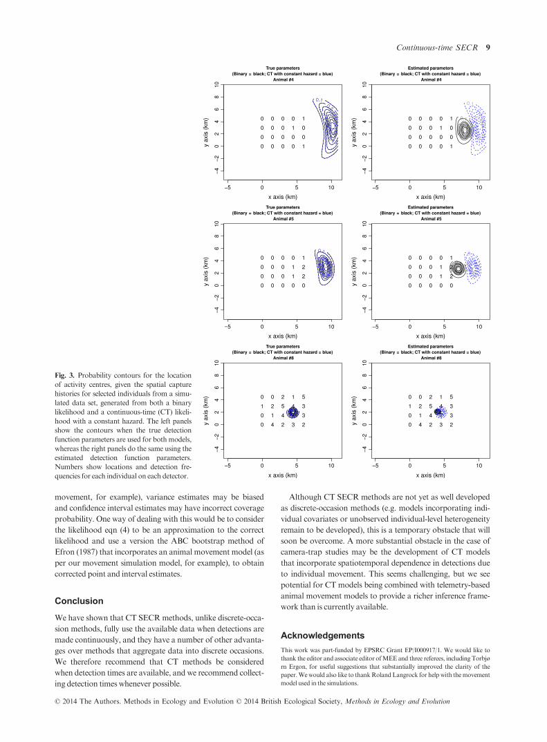
To understand this behaviour, we investigated simulated

data sets in which no count was greater than 1 in any interval.

The binary and CT estimators produced different estimates in

these cases, although they operate on identical data. This is

because the binary likelihoodmodels the probability of at least

one detection in an interval, whereas the CT likelihood models

the probability of exactly one detection, and the latter is more

informative about individual activity centre location. For

example, the fact that an individual was detected exactly once

by the detector suggests that the centre was not very close to

the detector (if it was, more than one detection would be

likely), whereas the fact that an individual was detected at least

once includes the possibility that it was detectedmany times, in

which case, the centre could be very close to the detector. Con-

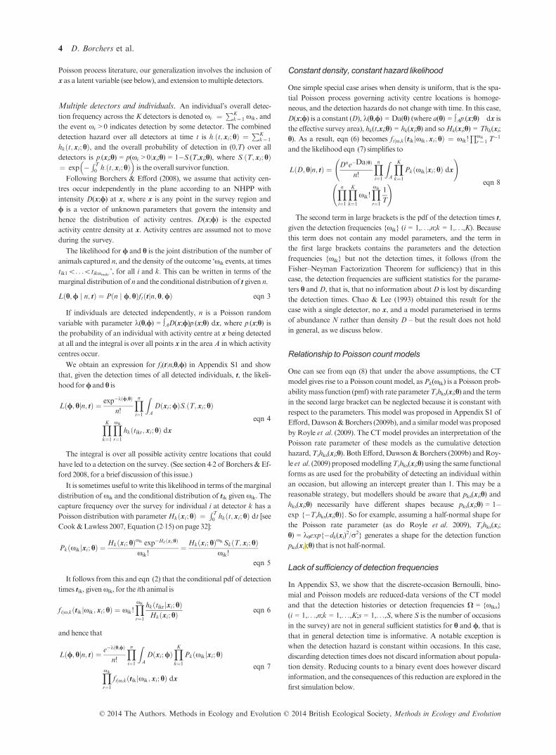
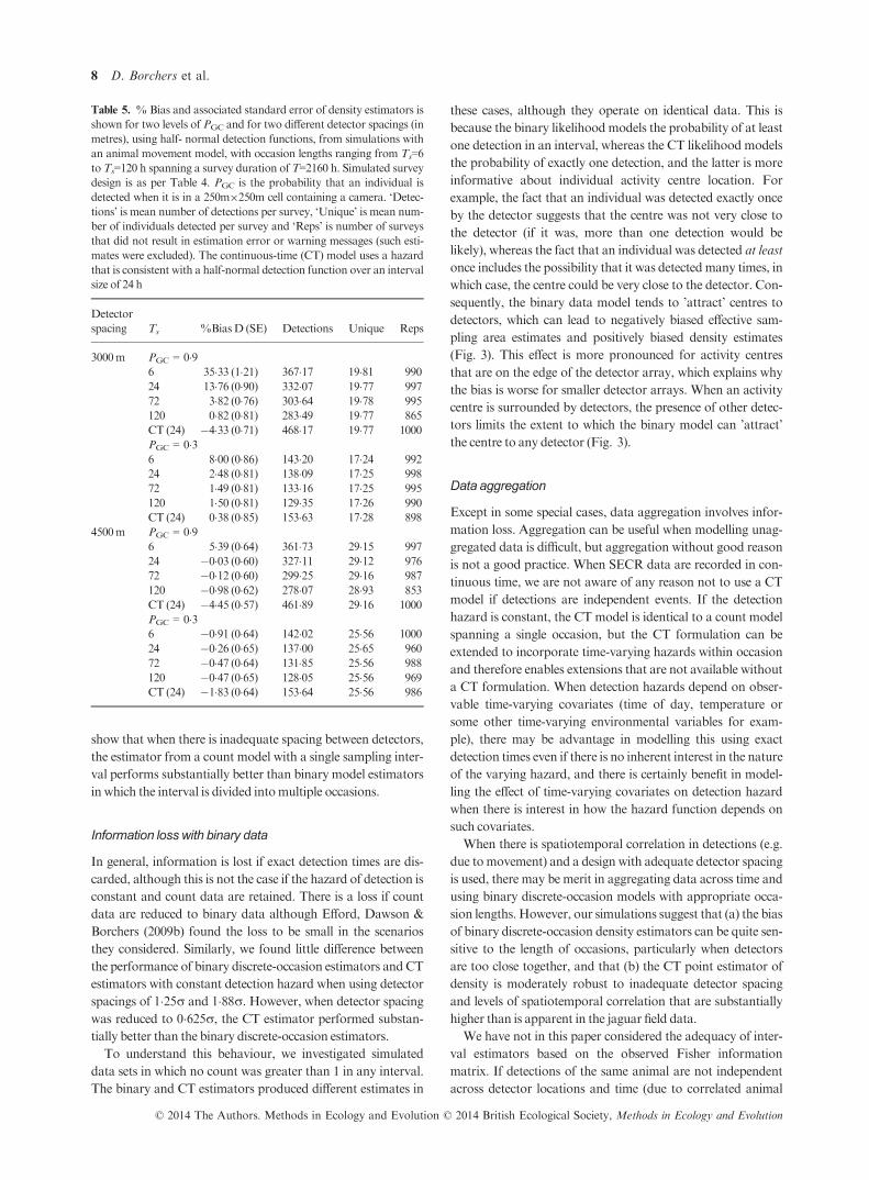
sequently, the binary data model tends to ’attract’ centres to

detectors, which can lead to negatively biased effective sam-

pling area estimates and positively biased density estimates

(Fig. 3). This effect is more pronounced for activity centres

that are on the edge of the detector array, which explains why

the bias is worse for smaller detector arrays. When an activity

centre is surrounded by detectors, the presence of other detec-

tors limits the extent to which the binary model can ’attract’

the centre to any detector (Fig. 3).

Data aggregation

Except in some special cases, data aggregation involves infor-

mation loss. Aggregation can be useful when modelling unag-

gregated data is difficult, but aggregation without good reason

is not a good practice. When SECR data are recorded in con-

tinuous time, we are not aware of any reason not to use a CT

model if detections are independent events. If the detection

hazard is constant, the CT model is identical to a count model

spanning a single occasion, but the CT formulation can be

extended to incorporate time-varying hazards within occasion

and therefore enables extensions that are not available without

a CT formulation. When detection hazards depend on obser-

vable time-varying covariates (time of day, temperature or

some other time-varying environmental variables for exam-

ple), there may be advantage in modelling this using exact

detection times even if there is no inherent interest in the nature

of the varying hazard, and there is certainly benefit in model-

ling the effect of time-varying covariates on detection hazard

when there is interest in how the hazard function depends on

such covariates.

When there is spatiotemporal correlation in detections (e.g.

due tomovement) and a design with adequate detector spacing

is used, there may be merit in aggregating data across time and

using binary discrete-occasion models with appropriate occa-

sion lengths. However, our simulations suggest that (a) the bias

of binary discrete-occasion density estimators can be quite sen-

sitive to the length of occasions, particularly when detectors

are too close together, and that (b) the CT point estimator of

density is moderately robust to inadequate detector spacing

and levels of spatiotemporal correlation that are substantially

higher than is apparent in the jaguar field data.

We have not in this paper considered the adequacy of inter-

val estimators based on the observed Fisher information

matrix. If detections of the same animal are not independent

across detector locations and time (due to correlated animal

Table 5. %Bias and associated standard error of density estimators is

shown for two levels of PGC and for two different detector spacings (in

metres), using half- normal detection functions, from simulations with

an animal movement model, with occasion lengths ranging from Ts=6to Ts=120 h spanning a survey duration of T=2160 h. Simulated survey

design is as per Table 4. PGC is the probability that an individual is

detected when it is in a 250m9250m cell containing a camera. ‘Detec-

tions’ is mean number of detections per survey, ‘Unique’ is mean num-

ber of individuals detected per survey and ‘Reps’ is number of surveys

that did not result in estimation error or warning messages (such esti-

mates were excluded). The continuous-time (CT) model uses a hazard

that is consistent with a half-normal detection function over an interval

size of 24 h

Detector

spacing Ts %BiasD (SE) Detections Unique Reps

3000m PGC = 096 3533 (121) 36717 1981 990

24 1376 (090) 33207 1977 997

72 382 (076) 30364 1978 995

120 082 (081) 28349 1977 865

CT (24) 433 (071) 46817 1977 1000

PGC = 036 800 (086) 14320 1724 992

24 248 (081) 13809 1725 998

72 149 (081) 13316 1725 995

120 150 (081) 12935 1726 990

CT (24) 038 (085) 15363 1728 898

4500m PGC = 096 539 (064) 36173 2915 997

24 003 (060) 32711 2912 976

72 012 (060) 29925 2916 987

120 098 (062) 27807 2893 853

CT (24) 445 (057) 46189 2916 1000

PGC = 036 091 (064) 14202 2556 1000

24 026 (065) 13700 2565 960

72 047 (064) 13185 2556 988

120 047 (065) 12805 2556 969

CT (24) 183 (064) 15364 2556 986

© 2014 The Authors. Methods in Ecology and Evolution © 2014 British Ecological Society, Methods in Ecology and Evolution

8 D. Borchers et al.

movement, for example), variance estimates may be biased

and confidence interval estimates may have incorrect coverage

probability. One way of dealing with this would be to consider

the likelihood eqn (4) to be an approximation to the correct

likelihood and use a version the ABC bootstrap method of

Efron (1987) that incorporates an animal movement model (as

per our movement simulation model, for example), to obtain

corrected point and interval estimates.

Conclusion

We have shown that CT SECRmethods, unlike discrete-occa-

sion methods, fully use the available data when detections are

made continuously, and they have a number of other advanta-

ges over methods that aggregate data into discrete occasions.

We therefore recommend that CT methods be considered

when detection times are available, and we recommend collect-

ing detection times whenever possible.

Although CT SECR methods are not yet as well developed

as discrete-occasion methods (e.g. models incorporating indi-

vidual covariates or unobserved individual-level heterogeneity

remain to be developed), this is a temporary obstacle that will

soon be overcome. A more substantial obstacle in the case of

camera-trap studies may be the development of CT models

that incorporate spatiotemporal dependence in detections due

to individual movement. This seems challenging, but we see

potential for CT models being combined with telemetry-based

animal movement models to provide a richer inference frame-

work than is currently available.

Acknowledgements

This work was part-funded by EPSRC Grant EP/I000917/1. We would like to

thank the editor and associate editor ofMEE and three referees, including Torbjø

rn Ergon, for useful suggestions that substantially improved the clarity of the

paper.Wewould also like to thankRolandLangrock for help with themovement

model used in the simulations.

Fig. 3. Probability contours for the location

of activity centres, given the spatial capture

histories for selected individuals from a simu-

lated data set, generated from both a binary

likelihood and a continuous-time (CT) likeli-

hood with a constant hazard. The left panels

show the contours when the true detection

function parameters are used for both models,

whereas the right panels do the same using the

estimated detection function parameters.

Numbers show locations and detection fre-

quencies for each individual on each detector.

© 2014 The Authors. Methods in Ecology and Evolution © 2014 British Ecological Society, Methods in Ecology and Evolution

Continuous-time SECR 9

Data accessibility

Data deposited in the Dryad repository: http://datadryad.org/resource/doi:10.

5061/dryad.mg5kv

References

Barbour, A.B., Ponciano, J.M. & Lorenzen, K. (2013) Apparent survival estima-

tion from continuous mark-recapture/resighting data.Methods in Ecology and

Evolution, 4, 846–853.Becker, N.G. (1984) Estimating population size from capture-recapture experi-

ments in continous time.Australian Journal of Statistics, 26, 1–7.Becker, N.G. & Heyde, C.C. (1990) Estimating population size from multiple

recapture experiments. Stochastic Processes and their Applications, 36, 77–83.Borchers, D. & Efford,M. (2008) Spatially explicit maximum likelihoodmethods

for capture-recapture studies.Biometrics, 64, 377–385.Borchers,D., Stevenson,B.,Kidney,D., Thomas, L.&Marques, T. (2013)Auni-

fying model for capture-recapture and distance sampling surveys of wildlife

populations. Journal of the American Statistical Association. doi: 10.1080/

01621459.2014.893884.

Boyce, M.S., Mackenzie, D.I., Manly, B.F., Haroldson, M.A. & Moody, D.

(2001) Negative binomial models for abundance estimation of multiple closed

populations. Journal ofWildlifeManagement, 65, 498–509.Caso, A., Lopez-Gonzalez, C., Payan, E., Eizirik, E., de Oliveira, T., Leite-Pit-

man, R.., Kelly, M. & Valderrama, C. (2008) Panthera onca. IUCN 2013. The

IUCN Red List of Threatened Species. Version 2013.2 <http://www.iucnred-list.org>Downloadedon21November 2013.

Chao, A. & Huggins, R. (2005) Modern closed-population capture-recapture

models. Handbook of Capture-recapture Analysis (eds S.C. Amstrup, T.L.

McDonald &B.F.J.Manly), chapter 4, pp. 58–87. PrincetonUniversity Press,

Princeton, NJ,USA.

Chao, A. &Lee, S.M. (1993) Estimating population size for continuous-time cap-

ture-recapturemodels via sample coverage.Biometrical Journal, 35, 29–45.Codling, E.A., Plank, M.J. & Benhamou, S. (2008) Random walks in biology.

Journal of the Royal Society Interface, 5, 813–834.Cook, R. & Lawless, J. (2007) The Statistical Analysis of Recurrent Events.

Springer, NewYork, NY,USA.

Craig, C.C. (1953) On the utilization of marked specimens in estimating popula-

tions of flying insects.Biometrika, 40, 170–176.Dawson, D.&Efford,M. (2009) Bird population density estimated fromacoustic

signals. Journal of Applied Ecology , 46, 1201–1209.Efford, M.G., Borchers, D.L. & Mowat, G. (2013) Varying effort in cap-

ture-recapture studies.Methods in Ecology and Evolution, 4, 629–636.Efford,M. (2004)Density estimation in live-trappingstudies.Oikos, 106, 598–610.Efford,M. (2013) secr: Spatially explicit capture-recapture models. R package ver-

sion 2.5.0.

Efford, M.G., Borchers, D.L. & Byrom, A.E. (2009a) Density estimation by spa-

tially explicit capture-recapture: Likelihood-based methods.Modelling Demo-

graphic Processes in Marked Populations (eds D. Thomson, E. Cooch & M.

Conroy), pp. 255–269. Springer, NewYork,NY,USA.

Efford, M.G., Dawson, D.K. & Borchers, D.L. (2009b) Population density esti-

mated from locations of individuals on a passive detector array. Ecology, 90,

2676–2682.Efron, B. (1987) Better bootstrap confidence intervals. Journal of the American

Statistical Association, 82, 171–200.Fewster, R. & Buckland, S. (2004) Assessment of distance sampling estimators.

Advanced Distance Sampling (eds S. Buckland, D. Anderson, K. Burnham, J.

Laake, D. Borchers & L. Thomas), chapter 10, pp. 281–306. Oxford Univer-

sity Press, Oxford,UK.

Foster, R.J. & Harmsen, B.J. (2014) Data from: Continuous-time spatially expli-

cit capture-recapture models, with an application to a jaguar camera-trap sur-

vey. Methods in Ecology and Evolution, Dryad Digital Repository.

doi:10.5061/dryad.mg5kv.

Foster, R.J. & Harmsen, B.J. (2012) A critique of density estimation from cam-

era-trap data.The Journal ofWildlifeManagement, 76, 224–236.Foster, R.J., Harmsen, B.J. & Doncaster, C.P. (2010) Habitat use by sympatric

jaguars andpumasacross agradientofhumandisturbance inbelize.Biotropica,

42, 724–731.Harmsen,B.J., Foster, R.J., Silver, S., Ostro, L.&Doncaster, C.P. (2010a)Differ-

ential use of trails by forest mammals and the implications for camera-trap

studies: a case study frombelize.Biotropica, 42, 126–133.Harmsen, B.J., Foster, R.J., Silver, S.C., Ostro, L.E. & Doncaster, C.P.(2010b)

The ecology of jaguars in the cockscomb basin wildlife sanctuary, Belize. The

Biology and Conservation of Wild Felids (eds D.W. MacDonald & A.J. Love-

ridge), chapter 18, pp. 403–416. OxfordUniversity Press, Oxford,UK.

Hwang, W. & Chao, A. (2002) Continuous-time capture-recapture models with

covariates.Statistica Sinica, 12, 1115–1131.Hwang, W., Chao, A. & Yip, P. (2002) Continuous-time capture-recapture mod-

els with time variation and behavioural response. Australian and New Zealand

Journal of Statistics, 44, 41–54.Langrock, R., King, R., Matthiopoulos, J., Thomas, L., Fortin, D. & Morales,

J.M. (2012) Flexible and practical modelling of animal telemetry data: hidden

markovmodels and extensions.Ecology, 93, 2336–2342.Lin, D.Y. &Yip, P.S.F. (1999) Parametric regressionmodels for continuous time

removal and recapture studies. Journal of the Royal Statistical Society: Series

B, 61, 401–411.Morales, J.M., Haydon, D.T., Frair, J., Holsinger, K.E. & Fryxell, J.M. (2004)

Extractingmore out of relocationdata: buildingmovementmodels asmixtures

of randomwalks.Ecology, 85, 2436–2445.Nayak, T. (1988) Estimating population size by recapture sampling. Biometrika,

75, 113–120.R Core Team. (2013) R: A Language and Environment for Statistical Computing.

R package version 3.0.2, Vienna, Austria.

Royle, J.A., Karanth, K.U., Gopalaswamy, A.M. & Kumar, N.S. (2009) Bayes-

ian inference in camera-trapping studies for a class of spatial capture-recapture

models.Ecology, 11, 3233–3244.Silver, S.C., Ostro, L.E.T., Marsh, L.K., Maffei, L., Noss, A.J., Kelly, M.J. et al.

(2004) The use of camera traps for estimating jaguar panthera onca abundance

anddensity using capture/recapture analysis.Oryx, 38, 148–154.Smouse, P.E., Focardi, Moorcroft, P.R., Kie, J.G., Forester, J.D. & Morales,

J.M. (2010) Stochastic modelling of animal movement. Philosophical Transac-

tions of the Royal Society B, 365, 2201–2211.Soisalo, M.K. & Cavalcanti, S.M.C. (2006) Estimating the density of a jaguar

population in the brazilian pantanal using camera-traps and capture-recapture

sampling in combination with gps radio-telemetry. Biological Conservation,

129, 487–496.Stuart, S.N., Chanson, J., Cox, N., Young, B., Rodrigues, A., Fischmann, D. &

Waller, R. (2004) Status and trends of amphibian declines and extinctions

worldwide.Science, 306, 1783–1786.Thompson, W. (2004) Sampling Rare or Elusive Species: Concepts, Designs, and

Techniques for Estimating Population Parameters. Island Press, Washington,

DC,USA.

Tobler, M.W. & Powell, G.V.N. (2013) Estimating jaguar densities with camera

traps: problems with current designs and recommendations for future studies.

Biological Conservation, 159, 109–118.Wilson, K.R. & Anderson, D.R. (1995) Continuous-time capture-recapture pop-

ulation estimation when capture probabilities vary over time. Environmental

and Ecological Statistics, 2, 55–69.Yip, P. (1989) An inference procedure for a capture and recapture experiment

with time-dependent capture probabilities.Biometrics, 45, 471–479.Yip, P.S.F., Huggins, R.M. & Lin, D.Y. (1995) Inference for capture-recapture

experiments in continuous time with variable capture rates. Biometrika, 83,

477–483.Yip, P.S.F. & Wang, Y. (2002) A unified regression model for recapture studies

with random removals in continuous time.Biometrics, 58, 192–199.Yip, P., Zhou, Y., Lin, D. & Fang, X. (1999) Estimation of population size based

on additive hazards models for continuous-time recapture experimets. Biomet-

rics, 55, 904–908.

Received 26 September 2013; accepted 18March 2014

Handling Editor: Robert B. O’Hara

Supporting Information

Additional Supporting Information may be found in the online version

of this article.

Appendix S1. Continuous-time proximity likelihood derivation.

Appendix S2. Discrete-occasion proximity likelihood derivation.

Appendix S3. Lack of sufficiency ofΩ.

© 2014 The Authors. Methods in Ecology and Evolution © 2014 British Ecological Society, Methods in Ecology and Evolution

10 D. Borchers et al.

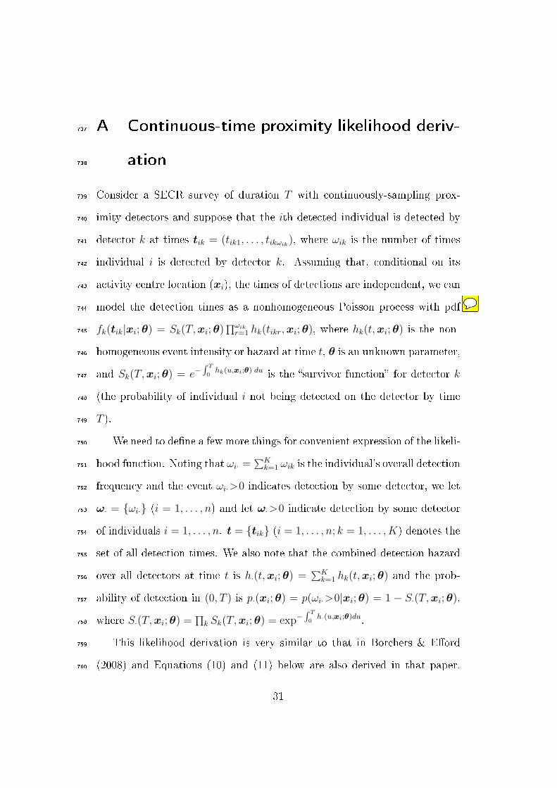
A Continuous-time proximity likelihood deriv-737

ation738

Consider a SECR survey of duration T with continuously-sampling prox-739

imity detectors and suppose that the ith detected individual is detected by740

detector k at times tik = (tik1, . . . , tikωik), where ωik is the number of times741

individual i is detected by detector k. Assuming that, conditional on its742

activity centre location (xi), the times of detections are independent, we can743

model the detection times as a nonhomogeneous Poisson process with pdf744

fk(tik|xi;θ) = Sk(T,xi;θ)∏ωikr=1 hk(tikr,xi;θ), where hk(t,xi;θ) is the non-745

homogeneous event intensity or hazard at time t, θ is an unknown parameter,746

and Sk(T,xi;θ) = e−∫ T

0hk(u,xi;θ) du is the survivor function for detector k747

(the probability of individual i not being detected on the detector by time748

T ).749

We need to dene a few more things for convenient expression of the likeli-750

hood function. Noting that ωi· =∑Kk=1 ωik is the individual's overall detection751

frequency and the event ωi·>0 indicates detection by some detector, we let752

ω· = ωi· (i = 1, . . . , n) and let ω·>0 indicate detection by some detector753

of individuals i = 1, . . . , n. t = tik (i = 1, . . . , n; k = 1, . . . , K) denotes the754

set of all detection times. We also note that the combined detection hazard755

over all detectors at time t is h·(t,xi;θ) =∑Kk=1 hk(t,xi;θ) and the prob-756

ability of detection in (0, T ) is p·(xi;θ) = p(ωi·>0|xi;θ) = 1 − S·(T,xi;θ),757

where S·(T,xi;θ) =∏k Sk(T,xi;θ) = exp−

∫ T

0h·(u,xi;θ)du.758

This likelihood derivation is very similar to that in Borchers & Eord759

(2008) and Equations (10) and (11) below are also derived in that paper.760

31

The reader may nd it useful to refer to Borchers & Eord (2008) when761

reading this derivation. We assume that, conditional on activity centre loca-762

tions of detected individuals (X = (x1, . . . ,xn)), the times and locations of763

detections of individuals are independent, and that individuals are detected764

independently. Suppose also that activity centres are realisations of a non-765

homogeneous Poisson process (NHPP) in the plane, with intensity D(x;φ)766

at x, and that φ is an unknown parameter vector. Then the likelihood for767

the parameters φ of the NHPP governing activity centre locations and the768

parameters θ of the detection process, is obtained from the pdf of the number769

of detected individuals n (P (n|φ,θ)), the pdf of the activity centre locations770

given detection (fX(X|ω·>0;φ,θ)), and the pdf of detection times t, given771

X and detection (ft(t|X,ω· > 0;θ)), after integrating over the unknown772

locations X, as follows:773

L(φ,θ|n, t) = P (n|φ,θ)ft(t|n,θ,φ)

= P (n|φ,θ)∫AfX(X|ω·>0;φ,θ)ft(t|X,ω·>0;θ) dX (9)

where774

P (n|φ,θ) =λ(θ,φ)ne−λ(θ,φ)

n!(10)

with λ(θ,φ) =∫AD(x;φ)p·(x;θ) dx (where the integral is over all points x775

in the area A in which activity centres occur), and776

fX(X|ω·>0;φ,θ) =n∏i=1

D(xi;φ)p·(xi;θ)

λ(θ,φ)(11)

32

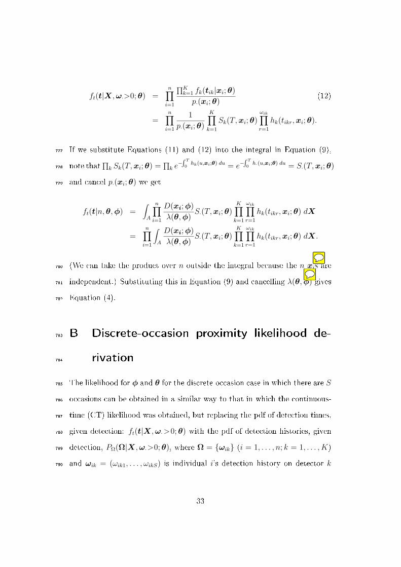
ft(t|X,ω·>0;θ) =n∏i=1

∏Kk=1 fk(tik|xi;θ)

p·(xi;θ)(12)

=n∏i=1

1

p·(xi;θ)

K∏k=1

Sk(T,xi;θ)ωik∏r=1

hk(tikr,xi;θ).

If we substitute Equations (11) and (12) into the integral in Equation (9),777

note that∏k Sk(T,xi;θ) =

∏k e−∫ T

0hk(u,xi;θ) du = e−

∫ T

0h·(u,xi;θ) du = S·(T,xi;θ)778

and cancel p·(xi;θ) we get779

ft(t|n,θ,φ) =∫A

n∏i=1

D(xi;φ)

λ(θ,φ)S·(T,xi;θ)

K∏k=1

ωik∏r=1

hk(tikr,xi;θ) dX

=n∏i=1

∫A

D(xi;φ)

λ(θ,φ)S·(T,xi;θ)

K∏k=1

ωik∏r=1

hk(tikr,xi;θ) dX.

(We can take the product over n outside the integral because the n xis are780

independent.) Substituting this in Equation (9) and cancelling λ(θ,φ) gives781

Equation (4).782

B Discrete-occasion proximity likelihood de-783

rivation784

The likelihood for φ and θ for the discrete-occasion case in which there are S785

occasions can be obtained in a similar way to that in which the continuous-786

time (CT) likelihood was obtained, but replacing the pdf of detection times,787

given detection: ft(t|X,ω·>0;θ) with the pdf of detection histories, given788

detection, PΩ(Ω|X,ω·>0;θ), where Ω = ωik (i = 1, . . . , n; k = 1, . . . , K)789

and ωik = (ωik1, . . . , ωikS) is individual i's detection history on detector k790

33

over the S occasions:791

L(φ,θ|n,ωik) = P (n|φ,θ)∫AfX(X|ω·>0;φ,θ)PΩ(Ω|X,ω·>0;θ) dX. (13)

This is the likelihood obtained by Borchers & Eord (2008).792

In 13 above PΩ(Ω|X;θ) is conditioned on being caught (ω·>0) and leads793

to another term entering the likelihood p.(x,θ)−1. Two forms of PΩ(Ω|X;θ)794

have been proposed for proximity detectors: one in which ωiks is binary,795

indicating detection or not of individual i on detector k on occasion s, and796

one in which ωiks is a count of the number of times individual i was detected797

by detector k on occasion s. Both have the form798

PΩ(Ω|X;θ) =n∏i=1

S∏s=1

K∏k=1

P (ωiks|xi;θ). (14)

The two forms of discrete-occasion SECRmodel dier in the form they use799

for P (ωiks|xi;θ). We show that when a CT detection process is discretised800

into discrete occasions this gives rise to a Bernoulli model in the case of801

binary data, and to binomial and Poisson SECR models in the case of count802

data. (Binomial and Poisson models have been proposed for the case in803

which there is only one occasion (S = 1) but are easily extended to multi-804

occasion scenarios, as we show below.) To do this, we divide the time interval805

(0, T ) into S subintervals with interval s running from ts−1 to ts, of length806

Ts = ts − ts−1, and with t0 = 0.807

With a CT model, the probability of detecting individual i at least808

once in detector k in this interval is pks(xi;θ) = 1 − e−Hks(xi;θ), where809

34

Hks(xi;θ) =∫ tsts−1

hk(u,xi;θ)du. Specifying a model for pks(xi;θ) implies810

a model for hk(t,xi;θ), although not a unique one. The mean value of the811

detection hazard in interval s must be hks(xi;θ) = − log 1− pks(xi;θ) /Ts812

and any hk(t,xi;θ) with this mean is consistent with pks(xi;θ). When813

the hazard is constant in the interval there is a one-to-one relationship814

between the detection hazard and the detection probability: hks(xi;θ) =815

− log 1− pks(xi;θ) /Ts.816

Bernoulli model This is obtained from a continuous-time model as PBern(ωiks|xi;θ) =817

pks(xi;θ)ωiks 1− pks(xi;θ)1−ωiks , with pks(xi;θ) = 1− e−Hks(xi;θ) and bin-818

ary ωiks.819

Binomial count model Eord, Dawson & Borchers (2009b) proposed this820

for the case in which the S original intervals are collapsed into S∗(< S) in-821

tervals and ωiks∗ is the count in the new interval s∗, which comprisesNs∗ adja-822

cent original intervals. In this case PBinom(ωiks∗ |xi;θ) =(Ns∗ωiks∗

)pks∗(xi;θ)ωiks∗ 1− pks∗(xi;θ)1−ωiks∗ ,823

where pks∗(xi;θ) = 1− e−Hks∗ (xi;θ), and Hks∗(xi;θ) =∑Ns∗s=1 Hks(xi;θ).824

Poisson count model A NHPP with intensity hk(t,xi;θ) at time t gives825

rise to an event count (ωiks) in a time interval (ts−1, ts) that has the Poisson826

pmf PP (ωiks|xi;θ) = Hks(xi;θ)ωiks exp−Hks(xi;θ) /(ωiks!), whereHks(xi;θ) =827 ∫ tsts−1

hk(u,xi;θ)du and event counts in non-overlapping intervals are inde-828

pendent.829

35

C Lack of suciency of Ω830

To investigate the suciency of Ω for the unknown parameters θ and φ, we831

consider the term fk(tik|xi;θ).832

The conditional distribution of detection times, t(s)ik = t

(s)ik1, . . . , t

(s)ikωiks

, in833

interval s, given that ωiks detections occurred in the interval is as follows:834

fts(t(s)ik |ωiks;θ) = ωiks!

ωiks∏r=1

hk(tikr,xi;θ)

Hks(xi;θ). (15)

We can now factorise fk(tik|xi;θ) into the pmf for the count ωiks in in-835

terval s and the pdf for the detection times, given the count, as follows:836

fk(tik|xi;θ) =S∏s=1

Hks(xi;θ)ωiks exp−Hks(xi;θ)

(ωiks!)

[ωiks!

ωiks∏r=1

hk(tikr,xi;θ)

Hks(xi;θ)

]

=S∏s=1

PP (ωiks|xi;θ)fts(t(s)ik |ωiks;θ) (16)

The likelihood Equation (4) can then be written as837

L(φ,θ|n, t) =e−λ(φ,θ)

n!

n∏i=1

∫AD(xi;φ)

K∏k=1

S∏s=1

PP (ωiks|xi;θ)fts(t(s)ik |ωiks;θ) dx(17)

The likelihood for the Poisson count model proposed by Eord, Dawson &838

Borchers (2009b) is this likelihood with a single occasion (S = 1) and without839

fts(t(s)ik |ωiks;θ)). It ignores the times of detection and because fts(t

(s)ik |ωiks;θ)840

involves θ, the detection frequencies alone (without the times of detection)841

are not in general sucient for θ. And because φ occurs in a product inside842

the integral, we can't factorise the likelihood into a component with φ and843

without t(s)ik , so that (by the Fisher-Neyman Factorization Theorem) Ω is844

36

neither sucient for θ nor φ. Finally, because neither the binomial nor the845

Bernoulli models involve the detection times, Ω is not sucient for θ and φ846

with any of these models either.847

There are two notable exceptions. The rst is when hk(t,xi;θ) is con-848

stant within intervals. In this case fts(t(s)ik |ωiks;θ) = ωiks!/T

ωikss , which849

does not involve θ (or the detection times) and so counts with the Poisson850

model are sucient for θ and φ. Note that in this case, the multi-occasion851

(S > 1) likelihood is identical to a single-occasion likelihood with occasion852

duration T =∑Ss=1 Ts (the only dierence being the multiplicative constant853

ωiks!/Tωikss ). A consequence of this is that when detection hazards do not854

depend on time, the notion of occasion is redundant when using a Poisson855

count model since the likelihood is identical whether or not it involves856

occasions.857

The second is when density is constant, i.e. D(x;φ) = D. In this case D858

can be factorised out of the integral and n is conditionally sucient for φ,859

given θ.860

37