ExpeER Distributed Infrastructure for EXPErimentation in

ExpeER - FP7 - 262060/ Data Management and policy

ExpeER

Distributed Infrastructure for EXPErimentation

in Ecosystem Research

Grant Agreement Number: 262060

SEVENTH FRAMEWORK PROGRAMME

Capacities

Integrating activities: Networks of Research Infrastructures(RIs)

Theme: Environment and Earth Sciences

DELIVERABLE 9.2

Assessment/review of model strengthens and weaknesses

Abstract:

The report summarises the work to provide Biogeochemical models potentially applicable at the EXPEER sites will be identified and evaluated with respect to strengths and weaknesses for modelling specific ecosystems, key ecosystem compartments as well as key drivers of change (e.g. climate and land use change). Also the ability to model vegetation change will be evaluated.

Due date of deliverable: M24 Actual submission date: M30

Start date of the project: December 1st, 2010 Duration: 48 months

Organisation name of lead contractor: DTU

Contributors: Claus Beier, Per Erik Jansson, Michael Michurov, Elianor Blyth

Revision N°: Final

Dissemination level:

PU Public (must be available on the website) [X]

PP Restricted to other programme participants (including the Commission Services) []

RE Restricted to a group specified by the consortium (including the Commission Services) (precise to whom it should be addressed)

[ ]

CO Confidential, only for members of the consortium(including the Commission Services) [ ]


Page 1 of 9

1 Executive summary

Three Biogeochemical models have been selected to be included in the EXPEER model toolbox. The model characteristics and specific features in terms of compartments and drivers are summarized in tables below.

2 Model selection

Three models have been identified and selected. These are COUP, LPJ-GUESS and JULES.

COUP model

Purpose: To quantify and increase the understanding concerning basic hydrological and biological processes in the soil-plant-atmosphere system. Brief Description : The model simulates soil water and heat processes in many type of soils; bare soils or soils covered by vegetation. The basic structure of the model is a depth profile of the soil. Processes such as snow-melt, interception of precipitation and evapotranspiration are examples of important interfaces between soil and atmosphere. Two coupled differential equations for water and heat flow represent the central part of the model. These equations are solved with an explicit numerical method. The basic assumptions behind these equations are very simple:

• (i) The law of conservation of mass and energy and

• (ii) flows occur as a result of gradients in water potential (Darcy's Law) or

temperature (Fourier's law).

The calculations of water and heat flows are based on soil properties such as: the water retention curve, functions for unsaturated and saturated hydraulic conductivity, the heat capacity including the latent heat at thawing/melting and functions for the thermal conductivity. The most important plant properties are: development of vertical root distributions, the surface resistance for water flow between plant and atmosphere during periods with a non limiting water storage in the soil, how the plants regulate water uptake from the soil and transpiration when stress occurs, how the plant cover influences both aerodynamic conditions in the atmosphere and the radiation balance at the soil surface. All of the soil-plant-atmosphere system properties are represented as parameter values. Meteorological data are driving variables to the model. Most important of those are precipitation and air temperature but also air humidity, wind speed and cloudiness are of great interest. Results of a simulation are such as: temperature, content of ice, content of unfrozen water, water potential, vertical and horizontal flows of heat and water, water uptake by roots, storages of water and heat, snow depth, water equivalent of snow, frost depth, surface runoff, drainage flow and deep percolation to ground water. In addition to the water and heat conditions also the plant dynamics and related turnover of nitrogen and carbon may be simulated. The abiotic and biotic processes may be linked in


Page 2 of 9

different ways also to handle the feedback between the physical driving forces and the plant development. A full technical description of the model is available as an Acrobat file. ftp://amov.ce.kth.se/CoupModel/CoupModel.pdf Contact: Prof. Dr. Per-Erik Jansson, KTH Royal Institute of Technology, Stockholm, Sweden; [email protected] References: Eckersten, H., Gärdenäs, A. & Jansson, P-E. 1995. Modelling Seasonal Nitrogen, Carbon,

Water and Heat Dynamics of the Solling Spruce Stand. Ecological Modelling, 83: 119-129 .

Jansson, P-E. & Thoms-Hjärpe, C. 1986. Simulated and measured soil water dynamics of unfertilized and fertilized barley. Acta Agric Scand 36:162-172.

Johnsson, H. & Jansson, P-E., 1991. Water balance and soil moisture dynamics of field plots with barley and grass ley. Journal of Hydrology, 129:149-173.

Stähli, M., Jansson, P.-E. & Lundin, L.-C. 1999. Soil moisture redistribution and infiltration in frozen sandy soils. Water Resources Research, 35 (1): 95-103.

LPJ-GUESS model

Purpose: LPJ-GUESS is a computer model that simulates the responses of land vegetation and ecosystems to climatic and environmental variation..

Brief Description: LPJ-GUESS model (Smith et al. 2001) employs forest-gap method to model dynamics of natural vegetation. Its implementation represents forest stand as a mosaic of independent patches each 1000 sq. m that are at different successional stages and follow independent hydrological and biogeochemical histories. The difference between the patches originates in explicitly-formulated processes of establishment, mortality and competition for resources under probabilistic disturbance regime. Overall state of the forest is obtained by averaging the patch variables. Establishment of new tree individuals occurs in age groups (“cohorts”), i.e. newly established individuals have similar characteristics; however, the age-dependent and growth-stress mortality of individual trees is modelled stochastically as is patch-destroying mortality due to a disturbance (e.g., storms, fire). Typically model is run with a daily time step, meaning that daily meteorological forcing data are required and most of the physiological processes are parameterised for this time scale. Establishment, growth, mortality and disturbances are calculated annually. Vegetation is organised into groups, referred to as plant functional types (PFTs), which have specific static parameters describing their ecological niches. List of PFTs is designed to represent most relevant and common plant species and live forms; it can be expanded or adjusted as necessary to account for site-specific vegetation.

The model was successfully applied to a variety of environments and a particular attention has been paid to European conditions with a more detailed parameterisation of the relevant PFTs (Wramneby et al. 2010; Smith et al. 2011). It was used with both historical meteorological datasets as well as various climate projections. Data from manipulation


Page 3 of 9

experiments were successfully used to evaluate obtained results at a wider regional or global scale (Hickler et al. 2008). Therefore, LPJ-GUESS is uniquely suitable to possible wide range of applications for ecosystem research in Europe.

Availability and documentation: The model is well documented and has a number of configuration parameters that can be adjusted by the users, including duration of the simulation and optional disturbance regime. The model, including a detailed description of the model is available at http://www.nateko.lu.se/lpj-guess Contact: Prof. Ben Smith, Dept of Physical Geography and Ecosystem Science, Lund University Geocentrum II. [email protected] References Hickler, T., B. Smith, I. C. Prentice, K. Mjöfors, P. Miller, A. Arneth and M. T. Sykes (2008).

"CO2 fertilization in temperate FACE experiments not representative of boreal and tropical forests". Global Change Biology 14(7): 1531-1542, doi: 10.1111/j.1365-2486.2008.01598.x.

Smith, B., I. C. Prentice and M. T. Sykes (2001). "Representation of vegetation dynamics in the modelling of terrestrial ecosystems: comparing two contrasting approaches within European climate space". Global Ecology and Biogeography 10(6): 621-637, doi: 10.1046/j.1466-822X.2001.t01-1-00256.x.

Smith, B., P. Samuelsson, A. Wramneby and M. Rummukainen (2011). "A model of the coupled dynamics of climate, vegetation and terrestrial ecosystem biogeochemistry for regional applications". Tellus A 63(1): 87-106, doi: 10.1111/j.1600-0870.2010.00477.x.

Wramneby, A., B. Smith and P. Samuelsson (2010). "Hot spots of vegetation-climate feedbacks under future greenhouse forcing in Europe". J. Geophys. Res. 115(D21): D21119, doi: 10.1029/2010jd014307.

JULES model Purpose: The Joint UK Land Environment Simulator (JULES) is a process-based model that simulates the fluxes of carbon, water, energy and momentum between the land surface and the atmosphere. Brief Description: JULES has a tiled model of sub-grid heterogeneity with separate surface temperatures, short-wave and long-wave radiative fluxes, sensible and latent heat fluxes, ground heat fluxes, canopy moisture contents, snow masses and snow melt rates computed for each surface type in a grid-box. Nine surface types are normally used: five Plant Functional Types (PFTs) - broadleaf trees, needleleaf trees, C3 (temperate) grass, C4 (tropical) grass and shrubs - and four non-vegetation types - urban, inland water, bare soil and land-ice. Except for those classified as land-ice, a land grid-box can be made up from any mixture of the other surface types. Fractions of surface types within each land-surface grid-box are read from an ancillary file or modelled by TRIFFID. Air temperature, humidity and wind-speed above the surface and soil temperatures and moisture contents below the surface are treated as homogeneous across a grid-box.


Page 4 of 9

The model runs on an hourly timestep with the incoming radiation energy being allocated to either sensible or latent heat fluxes from the land to the atmosphere as well as warming up the soil. Soil moisture dynamics are calculated using the Darcy-Richards equations with flow going across four vertically layered soils. If the soil moisture falls below a critical threshold, the transpiration is reduced and the photosynthesis is also reduced. The soil moisture also affects the surface and sub-surface runoff through a simple hydrology model. In this way, the carbon, water and energy cycles are linked. Availability and documentation: The model is freely available upon acceptance of the terms of conditions. Available at: https://jules.jchmr.org/ Contact: Eleanor Blyth - [email protected] References: Best, M. J., Pryor, M., Clark, D. B., Rooney, G. G., Essery, R .L. H., Ménard, C. B., Edwards, J.

M., Hendry, M. A., Porson, A., Gedney, N., Mercado, L. M., Sitch, S., Blyth, E., Boucher, O., Cox, P. M., Grimmond, C. S. B., and Harding, R. J.: The Joint UK Land Environment Simulator (JULES), model description – Part 1: Energy and water fluxes, Geosci. Model Dev., 4, 677-699, doi:10.5194/gmd-4-677-2011, 2011.

Clark, D. B., Mercado, L. M., Sitch, S., Jones, C. D., Gedney, N., Best, M. J., Pryor, M., Rooney, G. G., Essery, R. L. H., Blyth, E., Boucher, O., Harding, R. J., and Cox, P. M.: The Joint UK Land Environment Simulator (JULES), Model description – Part 2: Carbon fluxes and vegetation, Geosci. Model Dev. Discuss., 4, 641-688, doi:10.5194/gmdd-4-641-2011, 2011.


Page 5 of 9

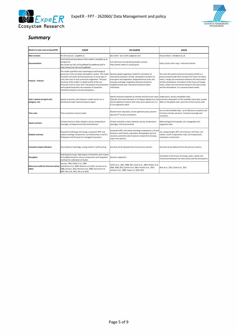
Summary Models for plot-scale testing (WP9) COUP LPJ-GUESS JULES

Main Contacts Per Erik Jansson - [email protected] Ben Smith - [email protected] Eleanor Blyth - [email protected]

Documentation

A full technical description of the model is available as an

Acrobat file.

ftp://www.lwr.kth.se/CoupModel/CoupManual.pdf or

http://www2.lwr.kth.se/CoupModel

Full reference list and demonstration version:

http://www.nateko.lu.se/lpj-guesshttps://jules.jchmr.org/ + references below

Purpose - features

The model quantifies basic hydrological and biological

processes in the soil-plant-atmosphere system. The model

simulates soil water and heat processes in many type of

soils; bare soils or soils covered by vegetation. The basic

structure of the model is a depth profile of the soil.

Processes such as snow-melt, interception of precipitation

and evapotranspiration are examples of important

interfaces between soil and atmosphere.

Dynamic global vegetation model for simulation of

interactions between climate, atmospheric burdens of

trace gases and vegetation, biogeochemical cycles and

trace gas exchange. Vegetation dynamics based on

neighbourhood-scale interactions between plant

individuals.

The Joint UK Land Environment Simulator (JULES) is a

process-based model that simulates the fluxes of carbon,

water, energy and momentum between the land surface

and the atmosphere. Simulation of the fluxes of energy,

water, carbon and momentum between the land surface

and the atmosphere. It is a process based model.

Scale / spatial unit (grid cells,

polygons, etc)

Spatial resolution: plot.However model can be run in

distributed model representing any region

Spatial resolution depends on climate and land cover input.

Typically 10 minutes (Europe) or 0.5 degree (globe) but may

also be applied at stand or plot scale, basic spatial unit is a

0.1 ha vegetation patch

Single point, country and global scale,

resolution dependent on the available input data; usually

50km on the global scale, and 1 km on the country scale

Time units Time resolution: hourly to dailyShortest time-step daily; can be applied to past, present-

day and 21st century simulations

be run with available data – up to 100 years in practice and

for future climate scenarios. Temporal coverage and

resolution

Inputs summaryClimate (hourly or daily radiation, precip, temperature

(average), windspeed and CO2 concentration)

Climate (monthly or daily radiation, precip, temperature

(average), CO2 concentration

Meteorological forcing data, soil, topography and

vegetation data

Outputs summary

Ecosystem hydrology and energy, ecosystem NPP, and

carbon exchange components, soil and biomass C and N ),

N deposion and N inputs for managed ecosystems

Ecosystem NPP, and carbon exchange components, soil and

biomass C and N pools, population demography and size

structure, potential natural species composition (Europe,

major tree species)

LAI, canopy height, GPP, soil moisture, leaf litter, soil

carbon, runoff, evaporation, heat, soil temperature,

respiration, momentum

Ecosystem impact indicators Any related to hydrology, energy and/or C and N cycling Any that can be deduced from the previous column. Any that can be deduced from the previous column.

Strengthes

Hydrology & energy. High degree of flexibility with respect

to feedback between various components and integrated

methods for calibration of model.

Dynamic vegetationSimulation of the fluxes of energy, water, carbon and

momentum between the land surface and the atmosphere

References (add full reference below

table)

Eckersten et al., 1995; Jansson et al, 1986; Johnsson and

Jansson, 1991; Stähli et al., 1999

Gustafsson et at, 2004; Hollesen et al 2011, Jannson et al,

2008, Jansson, 2012, Norman et al, 2008, Svensson et al

2007, Wu et al, 2011, Wu et al 2012

Smith et al., 2001, 2008, 2011; Sitch et al., 2003; Hickler et al.

2004, 2008, 2012; Zaehle et al. 2005; Arneth et al., 2007;

Lehsten et al., 2009; Tang et al. 2010, 2012

Best et al., 2011; Clark et al., 2011


Page 6 of 9

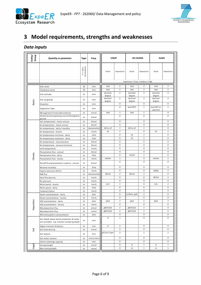
3 Model requirements, strengths and weaknesses

Data inputs

Enti

ty/

Gro

up

Quantity or parameter Type Freq.

In =

in

pu

t,

Va=

vali

dat

ion

Units Importance Units Importance Units Importance

Si te name ID once text 2 text 2 text 2

Treatment name ID once text 2 text 2 text 2

Si te Lati tude In oncedecimal

degree

2 decimal

degree

2 decimal

degree

2

Site Longitude In oncedecimal

degree

2 decimal

degree

2 decimal

degree

2

Elevation In once 0 0 0

Vegetation Type In once0 text (PFT) 1 text (PFT or

species )

1

Management his tory (description) In annual text 1 text 1 0

Start/end plant growing season/fumigation

periodIn Annual

0 0 0

Soi l temperature - mean annual In Annual 0 0 0

Air temperature - mean annual In Annual 0 0 0

Air temperature - da i ly / monthly In Daily/monthly dai ly, oC 2 dai ly, oC 2 0

Air temperature - hourly In hourly oC 2 0 oC 2

Air temperature minimum - da i ly In Daily 0 oC 2 0

Air temperature maximum - da i ly In Daily 0 oC 2 0

Air temperature - July maximum In Annual 0 0 0

Air temperature - January minimum In Annual 0 0 0

Leaf temperature In hourly 0 0 0

Precipi tation flux - annual In Annual 0 0 0

Precipi tation flux - da i ly In Daily 0 mm/d 2 0

Precipi tation flux - hourly In hourly mm/hr 2 0 mm/hr 2

Runoff flux (precipi tation surplus ) - annual In Annual0 0 0

Relative humidity In Daily 0 0 0

Vapour pressure defici t In hourly 0 0 kg/kg 2

PAR flux In daily/monthly W/m2 2 W/m2 2 0

Heat flux dens i ty In hourly 0 0 W/m2 2

Air pressure In hourly 0 0 0

Wind speed - hourly In hourly m/s 2 0 m/s 2

Wind speed - da i ly In Daily 0 0 0

Turbulent Stress In hourly 0 0 0

Ozone concentration - da i ly In daily 0 surface, ppb 2 0

Ozone concentration - hourly In hourly 0 0 0

CO2 concentration - da i ly In daily ppm 2 ppm 2 ppm 2

CO2 concentration - hourly In hourly 0 0 0

NHy depos i tion flux In annual gN/m2/yr 2 gN/m2/yr 2 0

NOx depos i tion flux In annual gN/m2/yr 2 gN/m2/yr 2 0

NH3 atmospheric concentration In daily 0 0 0

Soi l depth above which properties & s tocks

are recorded - e.g. solution sampl ing depthIn once

m 2 0 0

Organic horizon thickness In once m 2 0 0

Soi l bulk dens i ty In annual 2 0 0

Soi l texture In oncepF/soi l layer 2 1 1

Soi l water content In annual mean 0 0 0

Cation exchange capaci ty In once 0 0 0

Canopy height In annual 0 m 1 m 1

Max rooting depth In annual 0 m 1 m 1

COUP LPJ-GUESS

Bas

ics

Clim

ate

Dep

osi

tio

nSo

il

JULES

Importance - 0 low, 1 medium, 2 high

Veg

etat

ion


Page 7 of 9

En

tity

/

Gro

up

Quantity or parameter Type Freq.

In =

in

pu

t,

Va=

vali

dat

ion

Units Importance Units Importance Units Importance

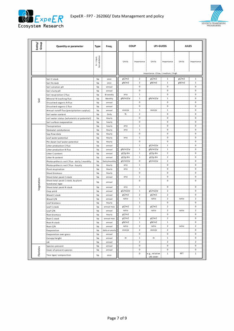
Soi l C s tock Va once gC/m2 2 gC/m2 1 gC/m2 1

Soi l N s tock Va once gN/m2 2 gN/m2 1 gN/m2 1

Soi l solution pH Va annual 0 0 0

Soi l s lurry pH Va annual 0 0 0

Soi l respiration C flux Va Bi-weekly any 1 0 0

Minera l N leaching flux Va Monthly gN/m2/yr 1 gN/m2/yr 1 0

Dissolved organic N flux Va annual 0 0 0

Dissolved organic C flux Va annual 0 0 0

Annual runoff flux (precipi tation surplus ) Va annual mm/yr 1 mm/yr 1 0

Soi l water content Va Daily % 2 0 0

soi l water s tatus (volumetric or potentia l ) Va Hourly 0 0 0

Soi l surface evaporation Va hourly 0 0 0

Transpiration Va hourly any 1 0 0

Stomatal conductance Va Hourly any 1 0 0

Sap flow data Va Hourly 0 0 0

Leaf water potentia l Va Hourly any 1 0 0

Pre-dawn leaf water potentia l Va Hourly 0 0 0

Litter production C flux Va annual 1 gC/m2/yr 1 0

Li tter production N flux Va annual gN/m2/yr 1 gN/m2/yr 1 0

Li tter C content Va annual gC/g dm 1 gC/g dm 2 0

Litter N content Va annual gC/g dm 1 gC/g dm 2 0

Photosynthes is net C flux - da i ly / monthly Va Daily/monthly gC/m2/yr 0 gC/m2/yr 2 0

Photosynthes is net C flux - hourly Va Hourly any 1 0 0

Plant respiration Va Hourly any 1 0 0

Shoot biomass Va Hourly 0 0 0

Shoot tota l peak C s tock Va annual any 1 0 0

Shoot tota l peak C s tock, by plant

functional typeVa annual

0 0 0

Shoot tota l peak N s tock Va annual any 1 0 0

Crop yield Va annual gC/m2/yr 1 gC/m2/yr 2 0

Wood C s tock Va annual gC/m2 2 gC/m2 2 0

Wood C/N Va annual ratio 1 ratio 2 ratio 2

Leaf biomass Va Hourly 1 0 0

Leaf C s tock Va annual max gC/m2 2 gC/m2 2 0

Leaf C/N Va annual ratio 1 ratio 2 ratio 2

Root biomass Va Hourly gC/m2 1 0 0

Root C s tock Va annual max gC/m2 2 gC/m2 2 0

Root N s tock Va annual gN/m2 1 gN/m2 1 0

Root C/N Va annual ratio 2 ratio 2 ratio 2

Evaporation Va daily or yearly mm/yr 2 mm/yr 2 0

Evaporation over grass Va annual 0 0 0

Canopy height Va annual m 1 m 1 0

LAI Va annual 2 2 2

Species present Va annual 0 0 0

Cover of present species Va annual 0 0 0

Tree type/ compos ition Va once0 e.g., relative

LAI cover

1 PFT 1

Flo

rist

ics

COUP LPJ-GUESS JULES

Importance - 0 low, 1 medium, 2 high

Soil

Veg

etat

ion


Page 8 of 9

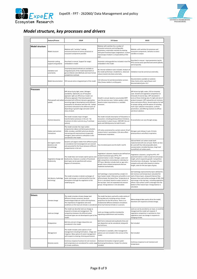
Model structure, key processes and drivers

Feature/Proces COUP LPJ Guess JULES

Model structure

Model structure

Modular with "switches" making

exclusion/inclusion of various processes or

ecosystem components possible

Modular with switches for a number of

ecosystem processes and configurable

parameters, extensible interface for dealing

with plant functional types (vegetation). Custom

input/output module is a responsibility of the

user.

Modular, with switches for processes and

ecosystem components. Switches to select

variables to output.

Parameter setting

support and guidance

Described in manual. Support for ranges

embedded in model

Parameter setting guidelines included in text file

embedded in the model

Described in manual. Input parameters (eg for

PFTs) can be easily specified and varied spatially

and temporally.

Validation and

uncertainty

Uncertainty based methods are available as

integrated parts of the model based both on

general Monte Carlo Methods and more formal

probabilistic methods

No internal validation tools included. Analysis of

the model performace (modelled vs. observed

values) needs to be done externally.

Validation must be carried out externally.

Model documentation Pdf manual and as integrated part of the modelFull reference list and demonstration version:

http://www.nateko.lu.se/lpj-guess

Documentation available on website:

https://jules.jchmr.org/software-and-

documentation/jules-v3.2

Processes

Plant growth and carbon

uptake

GPP driven by by light, water, Nitrogen

availability. Optionally use of Farquahar

approach, light use efficiency or water use

efficiency approach. Plant development

calculated with different dynamic approaches

assuming stage of development with different

seasonality for allocation and litter fall. Carbon

assimilation allocated to the different parts of

depending on growth stage and water and N

stress of plant.

Growth is annual, based on accumulated NPP

over the previous year. Carbon uptake is daily

based on plant requirements vs. available

resources.

GPP driven by light, water, CO2 on timestep

scale. Growth and vegetation competition on

timescale of several days. GPP calculated in

terms of three limiting rates: N, light and rate of

product transport. GPP reduced by soil moisture

stress and ozone effects. Several options for leaf

to canopy scaling, with the option of including

multi-layer radiation interception, sunfleck

penetration, and differing reactions to diffuse

and direct radiation.

Nutrient dynamics

The model includes major nitrogen

transformation processes in the soil. No

treatment of other nutrients (e.g. P and base

cations)

The model includes description of N dynamics in

ecosystem, including photosynthesis limitation,

accumulation in plant tissues. CENTURY-like soil

pools and SOM dynamics for both N and C.

N concetration can vary through canopy.

Carbon and nutrient

interactions

The model consider the major carbon

componentes (above and below ground plant,

SOM, microbes, and DOC) which are directly

interacting with macronutrients (especially

nitrogen), plant nutrient re-allocation is also

considered in the model.

C/N ratios constrained to a certain extent, N leaf

content limits C assimilation, C/N ratios affect

maintenance respiration.

Nitrogen cycle follows C cycle. N limits

photosynthesis and affects respiration.

Soil organic matter

dynamics and

microbiology

Dynamic soil organic matter from different pools

is considered. Soil microorganisms are covered

and accounted for the fluxes between different

compartments in the soil.

Two microbial pools exist for both C and N.

Q10 and RothC soil carbon model both

implemented with one soil pool. RothC can also

be used with four (decomposable plant,

resistant plant, microbial biomass, long-lived

humidified) soil carbon pools.

Vegetation change and

biodiversity

The model does not include explicit species and

biodiversity. However a number of functional

plant types can be specified with various

degrees of interactions.

Vegetation is dynamic, based on pre-defined set

of plant functional types (PFTs). PFT

parametrisation is static. Nitrogen, water and

light competition simmulated on individual or

PFT basis. Mortaliy includes both an age and a

growth-stress related components that are

modelled stochastically.

Vegetation is dynamic, using five PFTs. PFT

parameterisation is static except LAI and canopy

height, which respond to growth. Competition

hierarchy trees-shrub-grass. Two types of trees

compete with each other based on relative

height, same for the two types of grass.

Soil physics, hydrology

and energy

The model simulates in details exchanges of

water and energy in a vertical profile from the

atmosphere through the vegetation to the

underlying soil.

Soil hydrology is represented by a simple 2.5-

layer bucket model. Otherwise soil profile is not

differentiated. No lateral flow. Temperature at

25 cm is calculated, based on water content in

the top layer. Soils are separated into texture

groups. Energy balance is not calculated.

Soil hydrology represented by layers (default 4).

Soil moisture and temperature calculated for

each of these layers, along with Darcian flow

between them and surface exchange of H20, CO2

and energy in the top layer, including vegetation

effects. Sub-surface runoff is drainage from the

bottom of the lowest layer. Energy balance is

calculated.

Drivers

Climate change

The model simulate climate change (and

different climate scenarios), because

meteorological data are used as driving forces.

The importance of vegetation and snow

conditions on the local soil climate is considered.

The model has been used with a wide variety of

forcing data sets including various climate

projections for the XXI century. There is no

fundamental differens between simulations

driven by historical climate or a scenario.

Meteorological data used to drive the model,

therefore will respond to climate change.

Land use change

The model can describe land use change as

respond to climate and management. The

competition between the different plant

functional types are not developed as part of the

model.

Land-use change could be simulated by

regulating establishment and mortality.

Land use can be provided as an input, so could be

changed and the model will respond. If

vegetation competition is switched on, then

vegetation cover can change in response to

changing climate.

N depositionBoth dry and wet nitrogen deposition are

considered in the model.

Both forms (reduced and oxydised) of dry and

wet deposition can be considered, along with

the fertilisers.

Not included

Management

The model includes some options of soil

management including fertilization , tillage and

irrigation. Many options for plant management

with respect to clearing, thinning and harvest.

Fertilisation is available, other management

options are not included in this version of the

model.

Not included

Extreme events

Continous response functions for soil moisture

and temperature are considered for a wide range

of climate conditions.

Stochastic formulation of generic patch-

destroying disturbances. Simple fire scheme

included.

Continous response to soil moisture and

temperature


Page 9 of 9

4 Summary

Model selection

The model toolbox will contain three biogeochemical models. These were chosen among many possible obtions based on the following criteria:

Flexibility in terms of ecosystems and drivers

Documentation (manuals, user friendliness, access and references)

Complementarity (the three components of the model toolbox should ideally complement each other in terms of processes, drivers, ecosystems etc.)

Competences among the WP partners

Other models exist that could have fitted in as well, but no models have been identified which would have clear advantages over the ones chosen. Some ecosystem specific models for forests, grasses or agriculture might have advantages for those specific ecosystems, but would loose on the flexibility.

Parameter inputs

The models require a range of driving variables as well as characterising parameters and validation parameters. The driving variables are mostly climatic variables and management/treatments, which can be substantial, but which are required by any biogeochemical model, and they are more or less identical across the models.

Site characteristics and soil and plant parameters differ across models. These include quite many of which not all may be available at each site. Site specific solutions will have to be taken to obtain the parameters needed. The toolbox will provide guidelines for this.

Validation parameters will typically depend on the scientific question raised in a given project, and should therefore not be difficult to get from a given project. The toolbox will provide guidelines to more elaborate validation parameters.

Strengths

The different models are generally quite flexible with respect to terrestrial ecosystem types, they operate at slightly different scales and have different strengths. In combination this means that the model toolbox will provide models that together will provide useful model tools to cover most relevant ecosystem types and land uses, address key questions related to biogeochemical cycling and address questions at different time and spatial scales.

Key strengths are:

COUP – plot scale, soil hydrology & energy, C and N

LPJ-guess – Plot-regional scale, vegetation dynamics, atmospheric feedback

JULES – Landscape scale, hydrologic and carbon flows and feedbacks

Weaknesses

None of the models address other elements (like P and nutrients) or acidity

Documents

ExpeER Distributed Infrastructure for EXPErimentation in