Embed Size (px)
Citation preview

PARAXIAL APPLICATION OF AUXILIARY
DEVICES WITH WAVEGUIDE MEDIATED
LASER IRRADIATION FOR APPLICATIONS
IN MEDICAL BIOPHOTONICS
A Dissertation presented to
the Faculty of the Graduate School
at the University of Missouri
In Partial Fulfillment
of the Requirements for the Degree
Doctor of Philosophy
by
PAUL JAMES DOUGLAS WHITESIDE
Heather K. Hunt, Ph.D.
Dissertation Supervisor
May 2017

Declaration of ApprovalThe undersigned, appointed by the Dean of the Graduate School, have exam-
ined the dissertation entitled:
PARAXIAL APPLICATION OF AUXILIARY DEVICES WITH WAVEGUIDEMEDIATED LASER IRRADIATION FOR APPLICATIONS IN MEDICAL BIO-PHOTONICS
presented by Paul J.D. Whiteside, a candidate for the degree of Doctor of Philosophyin Bioengineering, and hereby certify that, in their opinion, it is worthy of acceptance.
Heather K. Hunt, Ph.D.
Sheila A. Grant, Ph.D.
Kevin D. Gillis, Ph.D.
Nicholas J. Golda, M.D.
John A. Viator, Ph.D.

Dedicated to my parents, Clive and Barbara Whiteside

“I may not have gone where I intended to go,but I think I’ve ended up where I needed to be”
The Long Dark Tea-Time of the Soul (1988)
– Douglas Adams
“No man is an island”
Meditation XVII (1624)
– John Donne

Acknowledgements
This research has been funded from a variety of sources, including partial fund-
ing from an NIH grant, the A. Ward Ford translational research grant, Wallace H.
Coulter Foundation translational research grant, and the MU Fast Track translational
research grant.
Throughout my graduate research career, there have been many people who
fundamentally contributed to my work either scientifically or morally, without whose
unique and invaluable contributions, this dissertation may never have successfully
come to fruition; whereas there have been others, whose proclivity for distraction and
knack for providing ample sources of extracurricular activities easily lengthened this
dissertation by a few years.
I would first like to thank my parents, Clive and Barbara Whiteside, for their
resolute and continuous support of my madness, because no one in their right mind
could ever justify intentionally choosing to get a Ph.D. Having such constant and
unwavering support was invaluable in finishing my continued education.
I would also like to thank Dr. Hunt and Dr. Viator, for giving me the freedom,
reassurance, and support to innovate new projects and technologies; and I’d like to
really thank Dr. Golda for somehow managing to coin a brilliantly catchy phrase for
yet another of my best inventions: Dr. Golda coined both “sonoillumination” and
“selective release waveguides.”
My projects have also benefitted from the technical and moral support of Dr.
Benjamin Goldschmidt, who helped to confirm that my mad ideas weren’t entirely
insane and might actually work out. Our approach to scientific research is funda-
mentally different, and for that I could not be more grateful, as it has led to more
constructive discourse than I enjoy with anyone else. Additionally, I have received
help and support from the likes of Quentin Bostick, Michael Carraher, Mason Schel-
lenberg, Jeff Chininis, Emma Bennett, Amanda Sain, Chenxi Qian, and Sharanya
Kumar, in addition to the services of the MU EMC and Mizzou Meat Market.
Finally, I would like to thank Dr. Ashley Ermer, who has been a constant source
of support and compassion, and who has complicated my life in all the best ways.
ii

Contents
Acknowledgements ii
List of Figures vii
List of Tables ix
Abbreviations x
Biological Terminology xii
Physical Constants xiii
Symbols xiv
Abstract xv
1 Introduction to biophotonics and waveguide-mediated irradiation 1
1.1 Applications of lasers in biophotonics . . . . . . . . . . . . . . . . . . 1
1.1.1 Selective photothermolysis . . . . . . . . . . . . . . . . . . . . 3
1.1.2 Deep tissue thermal effects . . . . . . . . . . . . . . . . . . . . 5
1.2 Laser-tissue interactions . . . . . . . . . . . . . . . . . . . . . . . . . 7
1.3 Modern methods in biophotonics . . . . . . . . . . . . . . . . . . . . 11
1.3.1 Common practices . . . . . . . . . . . . . . . . . . . . . . . . 11
1.3.2 Concerns regarding contemporary systems . . . . . . . . . . . 13
1.3.2.1 Problems . . . . . . . . . . . . . . . . . . . . . . . . 14
1.3.2.2 Limitations . . . . . . . . . . . . . . . . . . . . . . . 16
1.4 Contact-based transmission modality . . . . . . . . . . . . . . . . . . 18
1.4.1 Prior Investigations . . . . . . . . . . . . . . . . . . . . . . . . 19
1.4.1.1 Preliminary Methods . . . . . . . . . . . . . . . . . . 21
1.4.1.2 Preliminary Results . . . . . . . . . . . . . . . . . . 23
1.4.2 Branching projects encompassed by this dissertation . . . . . 25
iii

Contents
2 Techniques and challenges of metal thin film characterization forapplications in photonics 28
2.1 Introduction to metal films . . . . . . . . . . . . . . . . . . . . . . . 28
2.1.1 Importance of film thickness in optics . . . . . . . . . . . . . . 30
2.1.2 Metal thin film characterization . . . . . . . . . . . . . . . . . 33
2.2 Established characterization techniques . . . . . . . . . . . . . . . . . 35
2.2.1 X-Ray Reflectivity . . . . . . . . . . . . . . . . . . . . . . . . 37
2.2.1.1 XRR: Theory . . . . . . . . . . . . . . . . . . . . . . 37
2.2.1.2 XRR: Method . . . . . . . . . . . . . . . . . . . . . . 40
2.2.1.3 XRR: Analysis . . . . . . . . . . . . . . . . . . . . . 42
2.2.2 Ellipsometry . . . . . . . . . . . . . . . . . . . . . . . . . . . . 44
2.2.2.1 Ellipsometry: Theory . . . . . . . . . . . . . . . . . 44
2.2.2.2 Ellipsometry: Method . . . . . . . . . . . . . . . . . 46
2.2.2.3 Ellipsometry: Analysis . . . . . . . . . . . . . . . . . 48
2.2.3 Atomic Force Microscopy . . . . . . . . . . . . . . . . . . . . . 51
2.2.3.1 AFM: Theory . . . . . . . . . . . . . . . . . . . . . . 51
2.2.3.2 AFM: Method . . . . . . . . . . . . . . . . . . . . . 54
2.2.3.3 AFM: Analysis . . . . . . . . . . . . . . . . . . . . . 55
2.2.4 Electron Beam Techniques . . . . . . . . . . . . . . . . . . . . 57
2.2.4.1 E-Beam Techniques: Theory . . . . . . . . . . . . . . 58
2.2.4.2 E-Beam Techniques: Method . . . . . . . . . . . . . 61
2.2.4.3 E-Beam Techniques: Cross-Sectional SEM Analysis . 63
2.2.4.4 E-Beam Techniques: SEM-EDS Analysis . . . . . . . 66
2.3 Characterization limitations & considerations . . . . . . . . . . . . . 68
2.3.1 Radiative absorption . . . . . . . . . . . . . . . . . . . . . . . 68
2.3.2 Sample conductivity . . . . . . . . . . . . . . . . . . . . . . . 69
2.3.3 Derived vs. measured thickness . . . . . . . . . . . . . . . . . 71
2.4 Conclusions and developing technologies . . . . . . . . . . . . . . . . 72
3 Selective release waveguides and contact-based laser irradiation oftissue 76
3.1 Introduction . . . . . . . . . . . . . . . . . . . . . . . . . . . . . . . . 76
3.2 Technical discussion . . . . . . . . . . . . . . . . . . . . . . . . . . . . 77
3.2.1 Operating conditions of planar optical waveguides . . . . . . . 78
3.2.1.1 Maxwell’s and Fresnel’s Equations . . . . . . . . . . 78
3.2.1.2 Snell’s Law . . . . . . . . . . . . . . . . . . . . . . . 86
3.2.1.3 Waveguide operation . . . . . . . . . . . . . . . . . . 89
3.2.2 Evanescent fields and optical tunneling . . . . . . . . . . . . . 93
3.2.2.1 Evanescent fields . . . . . . . . . . . . . . . . . . . . 94
3.2.2.2 Frustrated total internal reflection . . . . . . . . . . 99
3.2.3 Contact-based transmission . . . . . . . . . . . . . . . . . . . 104
3.2.4 Objectives . . . . . . . . . . . . . . . . . . . . . . . . . . . . . 106
iv

Contents
3.3 Materials and methods . . . . . . . . . . . . . . . . . . . . . . . . . . 108
3.3.1 Porcine tissue samples . . . . . . . . . . . . . . . . . . . . . . 108
3.3.2 Waveguide fabrication . . . . . . . . . . . . . . . . . . . . . . 109
3.3.3 Experimental apparatus . . . . . . . . . . . . . . . . . . . . . 111
3.3.4 Experimental methodology . . . . . . . . . . . . . . . . . . . . 113
3.4 Results . . . . . . . . . . . . . . . . . . . . . . . . . . . . . . . . . . . 113
3.5 Discussion . . . . . . . . . . . . . . . . . . . . . . . . . . . . . . . . . 117
4 Simultaneous paraxial ultrasonic pulsation to improve transdermallaser fluence 119
4.1 Introduction . . . . . . . . . . . . . . . . . . . . . . . . . . . . . . . . 119
4.1.1 Objectives . . . . . . . . . . . . . . . . . . . . . . . . . . . . . 124
4.2 Phenomenological model . . . . . . . . . . . . . . . . . . . . . . . . . 126
4.2.1 Established acousto-optic theory . . . . . . . . . . . . . . . . . 126
4.2.2 Established UOT theory . . . . . . . . . . . . . . . . . . . . . 130
4.2.3 Mechanisms of sonoillumination . . . . . . . . . . . . . . . . . 131
4.2.3.1 Refractive index modulation . . . . . . . . . . . . . . 132
4.2.3.2 Alteration of optical collision events . . . . . . . . . 134
4.3 Materials and methods . . . . . . . . . . . . . . . . . . . . . . . . . . 139
4.3.1 Porcine tissue samples . . . . . . . . . . . . . . . . . . . . . . 139
4.3.2 Waveguide fabrication . . . . . . . . . . . . . . . . . . . . . . 140
4.3.3 Experimental apparatus . . . . . . . . . . . . . . . . . . . . . 142
4.3.4 Ultrasonic Pulsation . . . . . . . . . . . . . . . . . . . . . . . 145
4.3.5 Experimental procedures . . . . . . . . . . . . . . . . . . . . . 147
4.4 Results . . . . . . . . . . . . . . . . . . . . . . . . . . . . . . . . . . . 148
4.4.1 Electrical Impedance Measurements . . . . . . . . . . . . . . . 148
4.4.2 Relationship between photocurrent and laser energy . . . . . . 153
4.4.3 Optical transmission enhancement . . . . . . . . . . . . . . . . 155
4.5 Discussion . . . . . . . . . . . . . . . . . . . . . . . . . . . . . . . . . 158
4.6 Conclusions and continued research . . . . . . . . . . . . . . . . . . . 164
5 Backward-mode waveguide-mediated photoacoustic tomography 166
5.1 Introduction . . . . . . . . . . . . . . . . . . . . . . . . . . . . . . . . 166
5.2 Technical discussion . . . . . . . . . . . . . . . . . . . . . . . . . . . . 169
5.2.1 Photoacoustics . . . . . . . . . . . . . . . . . . . . . . . . . . 170
5.2.2 Backward-mode transmission modality . . . . . . . . . . . . . 171
5.2.3 Technical objectives . . . . . . . . . . . . . . . . . . . . . . . . 174
5.3 Materials and methods . . . . . . . . . . . . . . . . . . . . . . . . . . 175
5.3.1 Porcine tissue preparation . . . . . . . . . . . . . . . . . . . . 175
5.3.2 Turbid tissue phantom design . . . . . . . . . . . . . . . . . . 176
5.3.3 Waveguide fabrication . . . . . . . . . . . . . . . . . . . . . . 177
5.3.4 Experimental apparatus . . . . . . . . . . . . . . . . . . . . . 179
v

Contents
5.3.4.1 Optical apparatus . . . . . . . . . . . . . . . . . . . 179
5.3.4.2 Electronic apparatus . . . . . . . . . . . . . . . . . . 181
5.3.4.3 Multiplexer design . . . . . . . . . . . . . . . . . . . 182
5.4 Results . . . . . . . . . . . . . . . . . . . . . . . . . . . . . . . . . . . 188
5.4.1 Preliminary results . . . . . . . . . . . . . . . . . . . . . . . . 189
5.4.2 2D Depth Profiling . . . . . . . . . . . . . . . . . . . . . . . . 190
5.5 Discussion . . . . . . . . . . . . . . . . . . . . . . . . . . . . . . . . . 191
6 Conclusions & continued investigations 195
6.1 Conclusions . . . . . . . . . . . . . . . . . . . . . . . . . . . . . . . . 195
6.2 Continued investigations . . . . . . . . . . . . . . . . . . . . . . . . . 197
6.2.1 Project: Selective-release waveguides . . . . . . . . . . . . . . 197
6.2.2 Project: Sonoillumination . . . . . . . . . . . . . . . . . . . . 199
6.2.3 Project: Waveguide-mediated PAT . . . . . . . . . . . . . . . 201
A Derivation of Theoretical Equations 203
A.1 Maxwell’s Equations . . . . . . . . . . . . . . . . . . . . . . . . . . . 203
A.1.1 Wave Equation in terms of E . . . . . . . . . . . . . . . . . . 203
A.1.2 Wave Equation in terms of H . . . . . . . . . . . . . . . . . . 207
A.1.3 Characteristic Optical Admittance, Y . . . . . . . . . . . . . . 208
A.1.4 The Poynting Vector, Irradiance, and the Optical AbsorptionCoefficient . . . . . . . . . . . . . . . . . . . . . . . . . . . . . 211
A.1.5 Snell’s Law . . . . . . . . . . . . . . . . . . . . . . . . . . . . 213
A.2 Boundary conditions . . . . . . . . . . . . . . . . . . . . . . . . . . . 215
A.2.1 Normal incidence in non-absorbing media . . . . . . . . . . . . 215
A.2.2 Oblique incidence in non-absorbing media . . . . . . . . . . . 218
A.2.2.1 p-polarized light (TM polarized) . . . . . . . . . . . 218
A.2.2.2 s-polarized light (TE polarized) . . . . . . . . . . . . 223
A.2.2.3 Optical admittance for oblique incidence . . . . . . . 227
A.2.2.4 The Brewster Angle . . . . . . . . . . . . . . . . . . 229
B MATLAB Simulations 231
C Error Analysis of Labview-acquired data 235
C.1 Identifying sources of error . . . . . . . . . . . . . . . . . . . . . . . . 236
C.2 Error compensation . . . . . . . . . . . . . . . . . . . . . . . . . . . . 240
Bibliography 249
Vita 281
vi

List of Figures
1.1 Graph of Laser-Tissue Interactions . . . . . . . . . . . . . . . . . . . 3
1.2 Laser tattoo removal example: before and after . . . . . . . . . . . . 4
1.3 Diagram of fractional photothermolysis . . . . . . . . . . . . . . . . . 6
1.4 Photothermal effects within biological tissue . . . . . . . . . . . . . . 8
1.5 Cynosure MedLite C6 hand-piece . . . . . . . . . . . . . . . . . . . . 12
1.6 Original theoretical operation of contact-based transmission waveguides 20
1.7 Preliminary waveguide design . . . . . . . . . . . . . . . . . . . . . . 22
1.8 Preliminary apparatus utilized in M.S. Thesis work . . . . . . . . . . 23
1.9 Preliminary angular spectra of waveguides used in M.S. Thesis . . . . 24
2.1 Metal films utilized on planar waveguides . . . . . . . . . . . . . . . . 31
2.2 Importance of thickness for evanescent effects . . . . . . . . . . . . . 33
2.3 XRR theoretical diagram . . . . . . . . . . . . . . . . . . . . . . . . . 39
2.4 XRR equipment diagram . . . . . . . . . . . . . . . . . . . . . . . . . 41
2.5 XRR sample data analysis . . . . . . . . . . . . . . . . . . . . . . . . 42
2.6 Spectroscopic Ellipsometry equipment diagram . . . . . . . . . . . . . 47
2.7 Spectroscopic Ellipsometry sample data analysis . . . . . . . . . . . . 49
2.8 AFM theoretical diagram . . . . . . . . . . . . . . . . . . . . . . . . . 53
2.9 AFM equipment diagram . . . . . . . . . . . . . . . . . . . . . . . . . 54
2.10 AFM sample data analysis . . . . . . . . . . . . . . . . . . . . . . . . 56
2.11 E-beam interaction volume . . . . . . . . . . . . . . . . . . . . . . . . 59
2.12 SEM equipment diagram . . . . . . . . . . . . . . . . . . . . . . . . . 62
2.13 SEM sample data analysis . . . . . . . . . . . . . . . . . . . . . . . . 64
2.14 EDS sample data analysis . . . . . . . . . . . . . . . . . . . . . . . . 66
3.1 Oblique incidence sign conventions for TM and TE polarizations . . . 81
3.2 Fresnel Conditions . . . . . . . . . . . . . . . . . . . . . . . . . . . . 87
3.3 Reflectivity vs. Internal Reflection Angle: Glass–Air . . . . . . . . . . 91
3.4 Diagram of light propagation within a waveguide . . . . . . . . . . . 92
3.5 Reflectivity vs. Internal Reflection Angle: Glass–Silver . . . . . . . . 93
3.6 Evanescent field penetration depth: Glass–Air . . . . . . . . . . . . . 97
3.7 Evanescent field penetration depth . . . . . . . . . . . . . . . . . . . 98
vii

List of Figures
3.8 Diagram of Evanescent Penetration . . . . . . . . . . . . . . . . . . . 100
3.9 Diagram of Optical Tunneling . . . . . . . . . . . . . . . . . . . . . . 101
3.10 Boundary conditions for FTIR . . . . . . . . . . . . . . . . . . . . . . 102
3.11 Application of SRW in laser dermatology . . . . . . . . . . . . . . . . 106
3.12 SRW physical design . . . . . . . . . . . . . . . . . . . . . . . . . . . 109
3.13 Optical thin film regulation experimental apparatus . . . . . . . . . . 112
3.14 SEM-EDS analysis spectrum for Ag on Si substrate . . . . . . . . . . 114
3.15 Results of preliminary waveguide transmission experiments . . . . . . 116
3.16 Optical transmission through tissue vs. film thickness . . . . . . . . . 117
4.1 Graph of chromophore spectral absorption . . . . . . . . . . . . . . . 121
4.2 Sonoillumination modulating tissue . . . . . . . . . . . . . . . . . . . 125
4.3 Sonoillumination theoretical diagram . . . . . . . . . . . . . . . . . . 131
4.4 Porcine tissue sample cartridge . . . . . . . . . . . . . . . . . . . . . 140
4.5 Waveguide design for Sonoillumination applications . . . . . . . . . . 141
4.6 Experimental apparatus for Sonoillumination . . . . . . . . . . . . . . 142
4.7 3D printed optomechanical mount for Sonoillumination . . . . . . . . 144
4.8 Equivalent L-match circuit design . . . . . . . . . . . . . . . . . . . . 146
4.9 Resistance and reactance of the 500 kHz transducer . . . . . . . . . . 152
4.10 Graph of photocurrent vs. laser energy . . . . . . . . . . . . . . . . . 154
4.11 Graph of transmitted optical power by driving voltage . . . . . . . . 156
4.12 Sonoillumination improvement factor vs. driving voltage . . . . . . . 157
4.13 Resistance and reactance of an impedance matched transducer . . . . 159
4.14 Comparison of impedance magnitudes between transducer and matchedcircuit . . . . . . . . . . . . . . . . . . . . . . . . . . . . . . . . . . . 161
5.1 Waveguide-mediated photoacoustics . . . . . . . . . . . . . . . . . . . 172
5.2 Preliminary PAT waveguide design . . . . . . . . . . . . . . . . . . . 177
5.3 Optical apparatus of photoacoustic system . . . . . . . . . . . . . . . 179
5.4 3D printed photoacoustic tomography cartridge . . . . . . . . . . . . 180
5.5 Imasonic array transducer design . . . . . . . . . . . . . . . . . . . . 183
5.6 Multiplexer PCB design . . . . . . . . . . . . . . . . . . . . . . . . . 185
5.7 Photograph of the Multiplexer PCB . . . . . . . . . . . . . . . . . . . 186
5.8 Photograph of the completed multiplexer . . . . . . . . . . . . . . . . 188
5.9 Photoacoustic traces . . . . . . . . . . . . . . . . . . . . . . . . . . . 190
6.1 Waveguides with multi-layer thin film claddings . . . . . . . . . . . . 198
6.2 Acoustic wedge for pulsing into tissue at an angle . . . . . . . . . . . 200
C.1 Error from pulse to pulse energy variation . . . . . . . . . . . . . . . 239
viii

List of Tables
2.1 Examples of metal films in optics and biophotonics . . . . . . . . . . 30
2.2 List of metal film characterization techniques . . . . . . . . . . . . . . 36
3.1 Tabulated atomic ratios and thicknesses for Ag and Ti films . . . . . 115
4.1 Theorized threshold frequencies for sonoillumination efficacy . . . . . 139
4.2 Tabulated transducer complex electrical impedance values . . . . . . 152
4.3 Photocurrent regression statistics . . . . . . . . . . . . . . . . . . . . 155
4.4 Tabulated amplification statistics by driving amplitude . . . . . . . . 163
5.1 Tabulated electronic components used for MUX boards . . . . . . . . 187
5.2 Calculated speed of sound in tissue phantoms . . . . . . . . . . . . . 192
ix

Abbreviations
AFM Atomic Force Microscopy
ATR Attenuated Total Reflection
CW Continuous Wave
DAQ Data Acquisition
EMC Electron Microscopy Core
Er:YAG Erbrium doped Yttrium Aluminum Garnet
FS Fused Silica
FTIR Frustrated Total Internal Reflection
GRIF Gradient Refractive Index Field
GRIN Graded Index
LASER Light Amplification by Stimulated Emission of Radiation
LASIK Laser-Assisted In Situ Keratomileusis
MRI Magnetic Resonance Imaging
MTZ MicroThermal Zone
N-BK7 Borosilicate Crown Glass
N-IR Near-Infrared
Nd:YAG Neodymium-doped Yttrium Aluminum Garnet
NOA 74 Norland Optical Adhesive # 74
OCA Optical Clearing Agent
OCT Optical Coherence Tomography
PAQT Photonic Ablation via Quantum Tunneling
PAS PhotoAcoustic Spectroscopy
x

Abbreviations
PAT PhotoAcoustic Tomography
PC PolyCarbonate
PEG Polyethylene Glycol
PMMA PolyMethylMethAcrylate (i.e. Acrylic)
PXI PCI extensions for Instrumentation
SEM Scanning Electron Microscopy
SRW Selective Release Waveguide
TE Transverse Electronic
TIR Total Internal Reflection
TIRPAS Total Internal Reflection PhotoAcoustic Spectroscopy
TIZ Targeted Irradiation Zone
TM Transverse Magnetic
TOC Tissue Optical Clearing
TOCD Tissue Optical Clearing Device
UOT Ultrasound-modulated Optical Tomography
UV Ultraviolet
xi

Biological Terminology
Collagen Structural protein giving skin its elasticity
Dermis Lower layer of skin containing blood vessels and hair follicles
Epidermis Outer layer of skin containing melanin
Fibroblasts Collagen producing cells
Fibroplasia Formation of fibrous tissue to create the extracellular matrix
Hyperpigmentation Dramatic relative increase in local melanin content
Hyperthermia Elevated body temperature due to failed thermoregulation
Hypopigmentation Dramatic relative decrease in local melanin content
Hypertrophic scar Raised scars that protrude and distort tissue topography
Inflammation The body’s response to harmful stimuli and damage
Lymphatic system Vessels that transport constituents of the inflammatory response
Melanin Broadly optically absorbing pigment in skin and hair
Melasma Brown or grey-brown patches of discoloration in skin
Necrosis Cell death that releases cell contents into extracellular matrix
Oedema Area of fluid retention causing tissue swelling
Phagocytosis Process by which a cell engulfs a solid particle
Port wine stain Reddish area of capillary malformation in the skin
Purpura Red or purple discolorations in the skin
Thermal coagulation Denaturation of blood cells through intense heat
Vascular system System of vessels and capillaries through which blood flows
Vascularization Formation of blood vessels and capillaries in living tissue
White blood cell Cells responsible for engulfing and removing foreign elements
xii

Physical Constants
Speed of Light in a vacuum c = 2.9979 ×10⁸ m s−1
Speed of Sound in water vwater = 1.497 ×10³ m s−1
Speed of Sound in tissue vtissue = 1.470 ×10³ m s−1
Speed of sound in acrylic vacrylic = 2.750 ×10³ m s−1
Speed of sound in fused silica vFS = 5.960 ×10³ m s−1
Acoustic impedance of water Zwater = 1.483 ×10⁵ g /cm2 s−1
Acoustic impedance of tissue Ztissue = 1.580 ×10⁵ g /cm2 s−1
Acoustic impedance of acrylic Zacrylic = 3.260 ×10⁵ g /cm2 s−1
Acoustic impedance of fused silica Zfs = 13.1 ×10⁵ g /cm2 s−1
Refractive index of silver (532 nm) nAg = 0.1429
Refractive index of titanium (532 nm) nT i = 2.479
Refractive index of acrylic (532 nm) nacrylic = 1.4953
Refractive index of fused silica (532 nm) nFS = 1.4607
Extinction coefficient of silver (532 nm) kAg = 3.0518
Extinction coefficient of titanium (532 nm) kT i = 3.3511
Permittivity of free space ε0 = 8.8541 ×10⁻¹² m−3 kg−1 s4 A2
Permeability of free space µ0 = 1.2566 ×10⁻⁶ m kg s−2 A−2
xiii

Symbols
N complex refractive index (unitless)
n real component of N (unitless)
k complex component of N (unitless)
λ wavelength nm
P power mW (mJ s−1)
I intensity mJ
H Magnetic field strength A m−1
B Magnetic flux density T
E Electric field strength V m−1
D Electric displacement V m−2
j Electric current density A m−2
ρ Electric charge density C m−3
σ Electric conductivity S m−1
µ permeability m kg s−2 A−2
ε permittivity m−3 kg−1 s4 A2
µr relative permeability m kg s−2 A−2
εr relative permeability m−3 kg−1 s4 A2
T Relative transmission coefficient (unitless)
R Relative reflection coefficient (unitless)
Γg Gruneissen coefficient (unitless)
HB Radiant beam exposure J cm−2
Z Electrical Impedance Ω
xiv

UNIVERSITY OF MISSOURI
Paraxial application of auxiliary deviceswith waveguide mediated laser irradiationfor applications in medical biophotonics
Paul James Douglas Whiteside
Heather K. Hunt, Dissertation Supervisor
Abstract
Laser-based medical applications offer minimally-invasive alternatives to tradi-
tional procedures; however, the simplistic method of open-air laser transmission poses
ocular hazards and negative side effects, along with a fundamentally limited efficacy
for patients of darker complexion due to strong optical absorption in the epidermis.
Additionally, the traditional irradiation method also inhibits the incorporation of
additional technologies that might otherwise enhance therapeutic effects or provide
diagnostic benefits, as doing so would otherwise occlude the laser beam path. The
research presented herein addresses each of these considerations individually, first
by transmitting laser light into tissue through direct contact with a selective-release
waveguide, and thereafter incorporating auxiliary equipment on its rear face. Metal
clad planar optical waveguides are demonstrated for the transmission of laser light
into samples of porcine skin through direct transmission, governed by scaling evanes-
cent leaking through a designated active area by controlling thin film thickness. In
one manifestation, an ultrasonic pulser was incorporated to modulate tissue optical
properties and thereby improve transmission of light through epidermal and dermal
tissues by increasing forward anisotropy; whereas in another, a high frequency ul-
trasonic transducer was incorporated to detect photoacoustically generated pressure
waves to determine depth profiles of chromophores in skin as a foundation for clinical
backward-mode photoacoustic tomography.
xv

Chapter 1
Introduction to biophotonics andwaveguide-mediated irradiation
Portions of this chapter have been reproduced with permission from the Master’s
Thesis work entitled Photonic ablation via quantum tunneling, authored by Paul J.D.
Whiteside, Bioengineering Department, University of Missouri, May 2015 [1].
1.1 Applications of lasers in biophotonics
Although initially not intended for such applications, lasers have been incor-
porated into a wide variety of medical procedures, demonstrating strong appeal as
a highly controllable, non-invasive instrument. In particular, dermatology has been
among the most predominant fields with applications of lasers in medicine, including
tattoo removal, port wine stain treatment, skin resurfacing, treatment of acne vul-
garis, and ablation of vascular lesions and cancerous tumors [2–4]. However, while
many of the procedures are similar in nature, each of these applications requires the
use of a different variety of laser based primarily on the intended biological or chemical
target to be illuminated [5].
That being said, laser procedures in general can be broken down into five distinct
1

Chapter 1. Introduction
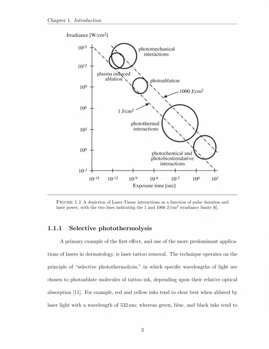
classifications, depending on the characteristics of the laser being utilized and the
duration of the laser pulse: photodisruption, plasma-induced ablation, photoablation,
thermal interaction, and photochemical interaction [6, 7]. The first three methods
utilize pulse durations in the range of femto- to nano-seconds, as shown in Figure
1.1, whereas the latter two employ durations in the millisecond to continuous wave
(CW) range. It is worth noting that although the shorter pulse durations do not
individually exhibit thermal effects identical to those produced using longer pulses,
similar results have been observed when the repetition rate of the laser and number
of pulses have been sufficiently high [8]. Consequently, in certain cases, short-pulse
duration approaches may be used for long-pulse duration applications; e.g. utilizing
short-pulse fractionated CO2 laser ablation for skin resurfacing.
However, while there are a plethora of applications for lasers in clinical derma-
tology, the method of choice for any given procedure generally reduces to one of two
principally desired effects – either the localized ablation of a target chromophore, or
the incitement of large area photothermal effects within the tissue. Principal exam-
ples of the former effect include the treatment of port wine stains, solar lentigines
(lesions), and pigmented tumors, along with the removal of percutaneous tattoos and
other foreign pigments [9–11]. By contrast, the latter effect typically encompasses
broad deep-tissue applications, such as acne scar treatment, skin resurfacing, and
hair removal [12–15].
2
Chapter 1. Introduction
Figure 1.1 A depiction of Laser-Tissue interactions as a function of pulse duration andlaser power, with the two lines indicating the 1 and 1000 J/cm2 irradiance limits [6].
1.1.1 Selective photothermolysis
A primary example of the first effect, and one of the more predominant applica-
tions of lasers in dermatology, is laser tattoo removal. The technique operates on the
principle of “selective photothermolysis,” in which specific wavelengths of light are
chosen to photoablate molecules of tattoo ink, depending upon their relative optical
absorption [11]. For example, red and yellow inks tend to clear best when ablated by
laser light with a wavelength of 532 nm; whereas green, blue, and black inks tend to
3

Chapter 1. Introduction
Figure 1.2 [left] Monochromatic tattoo prior to laser treatment. [right] The sametattoo after four treatments of 1064 nm laser light from a Q-Switched Nd:YAG laser with6 ns pulse duration [18].
clear best using 755 nm or 1064 nm [8, 16].
Unfortunately, there are currently no restrictions as to the chemical composition
of any tattoo inks, their pharmacological consistency, or their purity, the result of
which is that each pigment may necessitate a different wavelength based on the optical
absorption spectrum of the target ink, which may vary from patient to patient [17].
Additionally, the photoablation may also have adverse medical effects post-operation
due to the release of potentially harmful chemicals that previously comprised the
ink. For example, certain red inks tend to contain mercury or cadmium that may
be released into the body when the ink is ablated, which can result in a substantial
immunological response at the site of the tattoo or throughout the body [8].
Figure 1.2 demonstrates a comparison of the results of a series of four laser tat-
4

Chapter 1. Introduction
too removal treatments using a Q-switched Nd:YAG operating at 1064 nm. Although
individual treatments tend not to completely clear the tattoos, they are often prefer-
able to more invasive surgical procedures, which necessitate complex wound closing
procedures, potentially resulting in wound healing complications, hypertrophic scar-
ring, keloid formation, or anatomic distortion; consequently, laser tattoo removal
procedures generally consist of a lengthy series of treatments (between 4 - 20 treat-
ments depending on the complexity and size of the tattoo) [19–21]. Nevertheless,
laser tattoo removal has shown wider appeal and greater success than other treat-
ment procedures that tend to scar or injure the surrounding tissue, with methods
being refined and improved through medical laser research every year [22].
1.1.2 Deep tissue thermal effects
Another major application of lasers in dermatology is in the field of skin resur-
facing. Whereas tattoo removal procedures operate through photothermolysis, skin
resurfacing techniques capitalize on broader, deep-tissue photothermal effects in order
to achieve results. Laser skin resurfacing has fairly broad applications from acne scar
removal to skin tightening and wrinkle removal, but the general effect is the same
regardless of the structure to be resurfaced [23].
By utilizing relatively long pulse-widths (millisecond regime), the technique
focuses on the thermal interactions that occur in the area surrounding the illuminated
portion [15]. The high-energy laser light carbonizes and photocoagulates surface
tissue, causing necrosis in the top-most layer of the epidermis and an inflammatory
response in the deeper dermal tissue. The consequence of this photothermal damage
5

Chapter 1. Introduction
Figure 1.3 Fractional photothermolysis ablates columns of tissue to encourage collagenproduction in the dermis, without causing excess damage to the epidermis as in ablativeresurfacing techniques [27].
is that the scarred surface tissue is destroyed and subsequently removed, whereas the
deeper dermal tissue experiences an increase in collagen production to promote the
generation of well-structured, healthy tissue [24].
Unlike techniques that target specific pigmented chromophores, skin resurfacing
techniques target dissolved water molecules within the tissue; consequently, the lasers
used tend to operate in the IR or near-IR wavelength spectra, since water is strongly
optically absorbing in that range. The lasers typically used in skin resurfacing tend
to be CO2, Er:YAG, or Nd:YAG lasers with pulse durations from microseconds to
continuous wave [13, 25, 26].
Additionally, the techniques for laser skin resurfacing can be divided into three
categories – ablative resurfacing, nonablative dermal remodeling, and fractional pho-
tothermolysis – with each method focusing on a different aspect of the photothermal
response[27, 28]. Ablative resurfacing is primarily intended to evenly destroy surface
tissue, as shown in Figure 1.3 [left], and is useful for treating hypertrophic scarring
[24, 29]. Nonablative dermal remodeling, by contrast, focuses on homogeneously en-
6

Chapter 1. Introduction
couraging the increased production of collagen without causing excess surface tissue
damage, as shown in Figure 1.3 [center], and is useful for wrinkle removal procedures
[30].
Fractional photothermolysis, however, relies on the heterogeneous ablation of
tissue, leaving portions of healthy tissue interspersed between treated regions , as
shown in Figure 1.3 [right], and is used in the treatment of pigmented lesions,
melasma, and acne scarring [27, 31]. The intention of this approach is to cause
partial photothermolysis in the treated regions, referred to as “microthermal zones”
(MTZs), so as to achieve similar, albeit lessened, resurfacing effects as in ablative
resurfacing, while leaving the surrounding tissue to experience similar inflammatory
wound healing responses to those observed in nonablative dermal remodeling [24, 32].
Research has shown that Fractionated methods may result in faster recovery times
by reserving healthy tissue to more readily repair the laser-damaged tissue due to
keratinocyte diffusion from the untreated into the treated zones [4]. Additionally,
the non-ablative thermal damage to the surrounding tissue tightens and organizes
collagen fibers while simultaneously promoting neocollagen secretion by fibroblasts
[33, 34]. However, non-Fractionated methods are still widely used in treatments based
on manufacturers’ preferences and the relative youth of the Fractionated methods in
clinical applications.
1.2 Laser-tissue interactions
When examining the effects of laser light on biological tissue, there are a myriad
of considerations that may dramatically influence the final approach from an engineer-
7

Chapter 1. Introduction
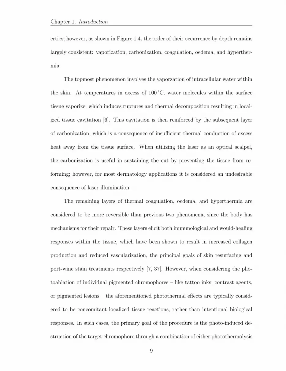
Figure 1.4 The severity of the thermal effects observed following illumination of biologicalsoft tissue with incident high-energy laser light decreases with penetration depth into thetissue [35].
ing perspective. Specific examples of such factors include inhomogenous scattering
and absorption within the tissue, the tissue’s density and water content, and the
degree of reflection at the surface of the tissue [35]. However, for dermatological
applications it is convenient to consider only the case of soft epithelial tissues like
skin. Whereas the specific effects will vary from person to person based on aspects
like melanin, fat, and water content, the resultant thermal effects within the tissue
remain largely consistent from person to person.
Regardless of the application, illuminating soft tissues with a high-powered laser
will result in a layering of distinct photothermal effects, resultant from the tissue’s
poor heat conductivity into the atmosphere coupled with its inherent thermal relax-
ation time [35, 36]. These effects differ between applications based on the laser’s
pulsewidth, energy density, and wavelength, along with the tissue’s own optical prop-
8
Chapter 1. Introduction
erties; however, as shown in Figure 1.4, the order of their occurrence by depth remains
largely consistent: vaporization, carbonization, coagulation, oedema, and hyperther-
mia.
The topmost phenomenon involves the vaporzation of intracellular water within
the skin. At temperatures in excess of 100 °C, water molecules within the surface
tissue vaporize, which induces ruptures and thermal decomposition resulting in local-
ized tissue cavitation [6]. This cavitation is then reinforced by the subsequent layer
of carbonization, which is a consequence of insufficient thermal conduction of excess
heat away from the tissue surface. When utilizing the laser as an optical scalpel,
the carbonization is useful in sustaining the cut by preventing the tissue from re-
forming; however, for most dermatology applications it is considered an undesirable
consequence of laser illumination.
The remaining layers of thermal coagulation, oedema, and hyperthermia are
considered to be more reversible than previous two phenomena, since the body has
mechanisms for their repair. These layers elicit both immunological and would-healing
responses within the tissue, which have been shown to result in increased collagen
production and reduced vascularization, the principal goals of skin resurfacing and
port-wine stain treatments respectively [7, 37]. However, when considering the pho-
toablation of individual pigmented chromophores – like tattoo inks, contrast agents,
or pigmented lesions – the aforementioned photothermal effects are typically consid-
ered to be concomitant localized tissue reactions, rather than intentional biological
responses. In such cases, the primary goal of the procedure is the photo-induced de-
struction of the target chromophore through a combination of either photothermolysis
9

Chapter 1. Introduction
or photoplasmolysis along with inelastic photoacoustic expansion (photomechanical
action), based on the pulse width and energy density of the laser [6].
Photothermolysis, as discussed in Section 1.1.1, is intended to break apart the
target chromophore into much smaller molecules by thermally compromising their
structural integrity. The effect is achieved by using ultra-short pulse durations in
the nanosecond regime to induce an acoustic shockwave, whose intensity exceeds the
fracture thresholds of the molecules [38]. The acoustic pressure wave is produced
through the rapid thermal expansion of the chromophore immediately following op-
tical absorption, in a process referred to as “photoacoustics.” Due to the extreme
energies of the incident beam, the photoacoustic expansion is inelastic, fragmenting
the target into smaller particles, which are more easily phagocytosed – engulfed by
white blood cells – for removal by the vascular or lymphatic systems [39]. Addition-
ally, the fragmentation of the chromophore may generate particles whose dimensions
are smaller than the wavelength of visible light, and would therefore be effectively
“cleared” regardless of their presence or absence in the tissue.
Photoplasmolysis acts in a similar fashion and produces a photoacoustic pressure
wave through the same inelastic expansion; however, the principal difference between
photoplasmolysis and photothermolysis is that the former effect results in the optical
breakdown and subsequent plasma formation by the target chromophore formed by
the ionizing effects of the incident beam [40–42]. Consequently, the ensuing explosive
inelastic expansion is much more extreme and results in a more thorough destruction
of the pigment [35]. The two effects are distinguished by the pulse width of the
incident beam, with photoplasmolysis exclusively occurring with pulse widths shorter
10

Chapter 1. Introduction
than 1000 ps and photothermolysis occupying the longer pulse width regime up to a
few hundred nanoseconds.
1.3 Modern methods in biophotonics
Regardless of the desired clinical effect, however, the means of tissue irradiation
in clinical practice is largely consistent across devices, with only slight differences
based on the intended application or the manufacturer’s proprietary designs. Al-
though the method is simple and straight-forward, it exposes the patient and practi-
tioner to significant hazards, while also being fundamentally limited in that it necessi-
tates a clear line of sight to the target, which precludes the incorporation of auxiliary
technologies.
1.3.1 Common practices
This method of laser transmission, which has been systematically accepted
throughout the clinical community, operates through the free-space open-air transmis-
sion of light aimed in the direction of the target tissue [43]. The techniques typically
involve routing the light into a tethered hand-piece by means of either a fiber-optic
bundle or an articulated mirror system, depending on the energy requirements of
the application. An adjustable lens within the hand-piece focuses the light onto the
tissue surface while the operating distance is set by an adjustable or interchangeable
stand-off or plastic guard, such as the thin metal stand-off attached to the end of the
hand-piece shown in Figure 1.5.
In addition to directing the laser light toward the tissue, medical laser man-
11

Chapter 1. Introduction
Figure 1.5 The Cynosure MedLite C6 laser system utilizes interchangeable hand-piecescontaining dye-doped modified polymers that increase the frequency of the Nd:YAG outputfrom 532 nm to either 585 or 650 nm for applications in selective photothermolysis [44, 45].
ufacturers may incorporate interchangeable hand-pieces to enhance the capabilities
of their systems. For example, a company called Cynosure currently produces the
MedLite C6 laser tattoo removal system, which is comprised of a powerful Q-Switched
Nd:YAG laser that is directed toward a hand-piece via an articulated mirror system
[45]. The Nd:YAG’s principal harmonic output is a beam of 1064 nm IR light; the
beam can also be frequency doubled to output the secondary harmonic beam at
532 nm in the visible spectrum. However, the MedLite C6 system, also incorporates
interchangeable hand-pieces, as shown in Figure 1.5, which contain dye-doped mod-
ified polymers. These polymers are pumped by the frequency doubled Nd:YAG in
order to output lower frequency beams. For example, a polymer within the hand-piece
doped with Pyrromethene-650 (PM-650) dye will output a beam at 650 nm, whereas
Pyrromethene-597 (PM-597) will output a beam at 585 nm [44]. Consequently, such
devices are primarily utilized in the selective photothermolysis of multi-colored tat-
12

Chapter 1. Introduction
toos for applications wherein the Nd:YAG’s harmonic outputs are insufficient (i.e.
for the ablation of chromophores that are not strongly absorbing at either 532 or
1064 nm).
Other companies produce similar units, each of which illuminates the tissue
through free-space delivery of light out of a hand-piece. The principal difference
between any two systems typically simplifies down to the lasing material (Nd:YAG,
Er:YAG, CO2, etc.), the pulse width, and the manufacturer’s proprietary technologies,
like the aforementioned dye-doped polymers. However, certain manufacturers also
incorporate a means of fractionating the beam out of the hand-piece for fractional
photothermolysis applications, as discussed in Section 1.1.2. For example, the Fraxel
Laser System, produced by Solta Medical, employs a CO2 laser that is directed into
a hand-piece wherein the beam is split up into an array of smaller beams to create
thousands of microthermal zones (MTZs) [46].
1.3.2 Concerns regarding contemporary systems
Although laser procedures have progressed substantially since the technology
was first put into practice by Leon Goldman in 1963, modern techniques still exhibit
many of the same detrimental characteristics as their forebears [9, 47, 48]. These
characteristics manifest as both distinctly detrimental operational hazards and fun-
damental limiting factors that compromise the efficacy of light-based medical proce-
dures. With regard to operational hazards, two of the more predominant problems
involve the risk of ocular injury to the practitioner and the potential for negative
tissue effects within the targeted tissue [49–52]. These concerns are directly resultant
13

Chapter 1. Introduction
from the operational design of the light delivery systems used in dermatology settings.
Moreover, all such designs regardless of application are subject to the same limitation,
in that they necessitate a clear line-of-sight to the optical target. This requirement
inhibits the incorporation of auxiliary devices, barring significant alteration to the
secondary technology, as the vast majority would otherwise occlude the path of the
light.
1.3.2.1 Problems
With regard to contemporary problems, the open-air, free-space delivery method
involves a distinct and consistent possibility for the un-confined light to reflect off the
patient’s skin. Considering that the vast majority of techniques utilize laser energies
between 1 and 1000 J/cm2, as per Figure 1.1, a diffuse reflection of even just 1% of
the incident energy may be enough to cause permanent eye damage to anyone present
[49]. This is particularly the case for ultra-short pulsed laser systems in the picosecond
to microsecond regimes, as the pulse can result in microcavitation or photoacoustic
destruction within retinal melanosomes, in addition to intra-retinal damage produced
through the ionizing effects of picosecond pulse lasers [53]. Moreover, it has been
reported that the vast majority of laser related injuries involve serious damage to the
retina, which consideration is only made worse by the extremely limited medical or
surgical treatments available to treat ocular laser injuries [49].
Consequently, in all dermatological laser applications, the practitioner and the
patient are required to wear protective eyewear with a high optical density for the
wavelength being used [54]. The high optical density reduces the degree to which
14

Chapter 1. Introduction
those wavelengths transmit into the retina; however, most eyewear occludes a broad
spectrum of wavelengths, rather than a single specific wavelength [55]. While these
glasses serve to protect the wearer from light-based injury, the high optical density
also dramatically hinders the vision of the laser operator across a broad spectrum
of wavelengths. Clinical practitioners therefore develop procedural habits wherein
they intermittently remove the eyewear between laser pulses so that they can visually
identify the target more clearly. This practice is currently a procedural necessity, due
to their limited vision; however, it entirely undermines the purpose of the protective
glasses in the event of a mistake.
Another consequence of the free-space propagation design is that the light is
transmitted into the skin at a tissue-air interface. As discussed in Section 1.2, the
poor heat conductivity at this interface prevents adequate heat dissipation, resulting
in carbonization, vaporization, and a subsequent inflammatory response. Whereas
most of these effects fade within a few days of treatment, more permanent hyper-
pigmentation, hypopigmentation, purpura, and scarring are possible side effects of
excessive damage or uneven wound healing [56]. Moreover, the potential for dam-
age increases noticeably for patients of darker skin phototypes (i.e. higher melanin
content or density), so much greater care must be taken for such patients [57, 58].
There are also other factors related to the delivery design that further exac-
erbate these problems. For example, there is a substantial degree of operator error
introduced because the hand-pieces are aimed at transdermal targets held suspended
above the tissue surface, which can result in harmful overexposure of the tissue,
causing permanent scarring and increased recovery times. Moreover, due to the in-
15

Chapter 1. Introduction
consistencies of the laser delivery methods and the rapid rate at which the oedema
forms within the tissue, most procedures necessitate a lengthy series of treatments,
rather than a single, more effective treatment, which only serves to compound the
aforementioned concerns with every subsequent visit, particularly in pigment clearing
procedures like tattoo removal [19, 21, 25].
1.3.2.2 Limitations
With regard to the incorporation of auxiliary devices, in order to utilize laser trans-
mission alongside any secondary technology, modern transmission modalities demand
that modifications be made to the secondary technique, which can often compromise
the effectiveness or otherwise require more complex alternatives to achieve the same
effect. One such example that has seen limited implementation in clinical laser der-
matology is the contact cooling of tissue during laser ablation procedures. In the
course of laser treatment, a significant amount of heat is generated through the unde-
sired optical absorption of the incident beam by biological chromophores within the
tissue (e.g. melanin, hemoglobin, water) [36]. This heating can permanently damage
tissue through carbonization and coagulation and is the primary source of pain during
procedures due to the thermal damage caused to local sensory nerves [6, 35]. Contact
cooling techniques have been suggested as a possible means of either mitigating this
thermal damage or otherwise cooling the tissue prior to the procedure to numb nerve
tissue and reduce patient pain [19]. However, contemporary methods of transmitting
laser light necessitate that cooling devices must not occlude the path of the beam.
This requirement has thus far effectively limited the viable options for cooling the
16

Chapter 1. Introduction
tissue during procedures to the use of cold air or cryogenic sprays, as cooling pads
would block the incident laser light [2, 28, 30, 59].
Another example of an application that attempts to incorporate laser irradia-
tion alongside additional equipment is in the field of photoacoustic tomography, which
involves the generation of ultrasonic pressure waves within tissue following the ab-
sorption of a sufficiently short pulse of light [60–62]. Due to factors such as acoustic
attenuation and impedance mismatches between soft and hard tissues, applications
of photoacoustics in a clinical setting necessitate that the acoustic detectors record
signals from the same side of the tissue from which they were generated, a condition
referred to as “backward mode.” This requirement has proven challenging to per-
form outside of a laboratory setting, since traditional ultrasonic transducers in this
orientation either occlude the path of the laser beam or otherwise must be positioned
off-axis. Nevertheless, as with the tissue cooling technologies, alternative approaches
have been developed that modify the secondary detection equipment in order to al-
low for a freely propagating laser beam. One such solution, presented by Zhang
et al. resolved the occlusion issue by utilizing a dual-wavelength optical method of
ultrasonic measurement [63]. The system utilizes two lasers of different wavelengths
superimposed on each other incident upon a Fabry-Perot (F-P) etalon manufactured
with dichroic films surrounding a compressible transparent polymer layer [64]. This
arrangement allows one of the beams to excite the photoacoustic response within the
tissue, while the other is used to record the interference response of the F-P cavity,
which varies as the thickness of the polymer layer is changed when the ultrasonic
pressure wave hits its surface. Similar F-P cavities have also been minimized to the
17

Chapter 1. Introduction
tip of a 125 µm optical fiber acting as an optical hydrophone, which can be positioned
in an array around a central illuminating optical fiber for photoacoustic generation
[65].
1.4 Contact-based transmission modality
Based on these examples, the standard approach to resolving the occlusion
problem observed in dual-technology systems typically involves modifying the sec-
ondary technology in order to accommodate a freely propagating laser beam, which
may place additional design constraints or limitations on their use. Meanwhile, the
standard approach to resolving the ocular hazards presented by reflections involves
the use of occluding eyewear, which presents issues in and of itself. These concerns
gave rise to the contact-based transmission modality around which this dissertation
is focused. The method, originally referred to as photonic ablation via quantum tun-
neling (PAQT), departs from traditional free-space propagation in favor of a thin
planar optical waveguide that delivers the light via direct physical contact with the
tissue. This method encloses the optical system, which circumvents hazards associ-
ated with backscattered light and prevents occlusion of the light while allowing for
the paraxial operation of a second technology on the rear face of the waveguide [66].
For example, in the case of photoacoustic tomography, a traditional piezoelectric ul-
trasonic transducer or array may be positioned on the rear face of the waveguide to
detect photoacoustic waves propagating out from the tissue, through the waveguide
substrate, toward the detector surface [67]. The modality was originally investigated
in my Master’s Thesis and forms the foundation for the various applications inves-
18

Chapter 1. Introduction
tigated in this Dissertation. The following sections provide a brief summary of the
prior research, which established the core principles of the technology.
1.4.1 Prior Investigations
The following sections cover the preliminary findings in the foundation of the
contact-based method as presented in the manuscript entitled Regulation of evanes-
cent leaking for contact-based light transmission in biophotonics applications, authored
by Paul J.D. Whiteside, Nicholas J. Golda, Randy D. Curry, and John A. Viator,
which has been submitted for publication in the journal Applied Optics [68].
For the purposes of this project, the PAQT waveguides consisted of glass slabs
clad in layers of titanium and silver. The waveguides also incorporated rectangular
“active areas” consisting of thin films of those same metals, which allow the light to
optically tunnel into tissue phantoms by means of evanescent leaking. The degree of
optical tunneling is strongly related to the incident angle of the light and the thickness
of the film in the active area, so waveguides were scanned throughout a range of
internal reflection angles using cylindrical coupling lenses, as shown in Figure 1.6,
and transmitted through films of four different thicknesses. The specific objectives of
this study were to:
• establish waveguide fabrication protocols;
• record a wide range of internal reflection geometries using hemi-cylindrical cou-
pling lenses;
• demonstrate laser beam transmission into agar gel tissue phantoms;
19

Chapter 1. Introduction
Figure 1.6 Coupling light directly into tissue by physical contact circumventsmany of the issues presented by free-space propagation techniques, and the use ofcylindrical coupling lenses permits tuning of the internal reflection angles.
• regulate transmission efficiency by varying active area film thickness.
The modality presented herein is heavily dependent upon both macroscale opti-
cal waveguide transmission along with the sub-wavelength evanescent effects demon-
strated by photons undergoing total internal reflection, which concepts will be dis-
cussed more thoroughly in Chapter 3. Optical waveguides are a well established
technology and have been used extensively in a variety of applications, including
optoelectronic integrated circuitry, attenuated total reflection spectroscopy (ATR),
and laser beam generation within planar waveguides [69–71]. Light is transmitted
along the length of the substrate by internally reflecting between their bounding sur-
faces, as a result of refractive index differences between substrate and cladding media.
Although most waveguides utilize polymer claddings (n2 ≥ 1.32) to ensure total inter-
20

Chapter 1. Introduction
nal reflection (TIR) conditions and permit waveguide operation, the objectives of this
study necessitated an uncommonly low critical angle, which could not be achieved
with any commercially available polymer. Consequently, the waveguides fabricated
for this project consisted of BK7 glass substrates (n1 = 1.519 at 532 nm) coated in
a layer of silver (n2 = 0.1429) applied using a cold sputter coater, resulting in an
extremely low critical angle, θc = 5.36°, permitting TIR within the waveguide for all
incident angles 6° < θ1 < 90° [72, 73].
In these experiments, laser light was coupled into a planar optical waveguide,
wherein it reflected between opposing faces until reaching a thin film active area.
When placed in contact with skin or a tissue phantom, the light at each internal
reflection point occurring within the active area either refracted or optically tunneled
into the external medium, depending on the active area film thickness.
1.4.1.1 Preliminary Methods
The waveguides developed for this study were fabricated in house, utilizing rectangu-
lar BK7 glass slabs 1 mm thick, clad in thick films of silver and titanium, as shown in
Figure 1.7. The former was chosen as a cladding due to its exceptionally low refrac-
tive index, n = 0.1429, at the lasing wavelength of 532 nm that was produced from
the second harmonic generator of a Q-switched Nd:YAG laser; whereas the latter was
deposited in an ultra-thin film to serve as an adhesion layer for the silver, since silver
does not strongly adhere to glass [73–75].The entrance aperture geometry measured
6 mm from the end of the substrate, which permitted the incorporation of a hemi-
cylindrical lens (Thorlabs, LJ1878L2-A) adhered atop the entrance aperture using
21

Chapter 1. Introduction
Figure 1.7 BK7 glass substrates were clad in thin films of Ti and Ag (shownexaggerated above), with a separately deposited active area on the underside of thesubstrate.
NOA 74 (Norland Optical Adhesive # 74). A section of the substrate was masked
off on the opposite face to serve as the active area, which was designed to begin at
approximately 21.10 mm from the aperture end of the slab and end at approximately
45.0 mm.
Synthetic multi-layered tissue phantoms composed of agar gel and optically
absorbing rubber were utilized in these experiments to simulate aspects of human
skin. A clear layer of agar separated the waveguide from the rubber absorber, which
was intended to represent a target chromophore, such as a blood vessel or cancerous
lesion, approximately 3 mm to 4 mm below the surface of the tissue. Rubber was
chosen as opposed to a dye or other such pigment to prevent the chromophore from
diffusing throughout the agar phantom.
A Q-switched Nd:YAG laser (Quantel, Brilliant B), which transmitted a verti-
cally polarized beam at a wavelength of 532 nm in a circular gaussian profile with a 5 ns
pulse width, was used to generate photoacoustic signals within the tissue phantom by
22

Chapter 1. Introduction
Figure 1.8 P-polarized light was directed into a beam dump (a), while s-polarizedlight transmitted through a 50:50 beamsplitter. Half of the energy directed towarda rubber chromophore adhered to an ultrasonic transducer (b) to measure incidentbeam energy, while a reflection was used to trigger a photodiode (d). Remain-ing light was transmitted into the tissue phantom via an optical waveguide to bedetected by an ultrasonic transducer (e) for photoacoustic signal analysis.
means of the waveguides developed for this study. Figure 1.8 depicts the optical train
used to couple light into the waveguides and demonstrates that the waveguides could
be rotated with respect to the incident beam to vary the internal reflection angle.
Photoacoustic signals generated within the tissue phantom were recorded throughout
the angular spectrum at 0.2° increments from perpendicular incidence to 75°. Tests
were repeated 15 times to improve statistical reliability.
1.4.1.2 Preliminary Results
Figure 1.9 depicts the integrated energy transmission curve throughout the angular
spectrum for each of the four active area geometries under consideration. Each of the
curves represents the respective mean corrected intensity spectrum calculated from
15 successive angular spectra recorded under identical situations without making any
alteration to the apparatus between tests. The angular spectra shown in Figure 1.9
23

Chapter 1. Introduction
0 10 20 30 40 50 60 70 800
0.5
1
1.5
2
2.5
3
3.5
Internal Reflection Angle (deg)
Aver
age
Corr
ecte
dIn
tensi
ty(a
.u.)
Integrated energy transmission vs. angle
TheoreticalCriticalAngle
BareTi + AgTi+Ag x2Ti+Ag x3
1
Figure 1.9 The decrease in integrated intensity corresponds with the decrease inevanescent penetration into tissue phantoms through silver films with increasingthickness.
demonstrate that the intensity of light transmitted into the phantom reached its
maximum near 50° and decreased with increasing film thickness. The diminishing
transmission was expected seeing as the bare active areas transmitted light through
the exposed glass substrate by means of simple refraction; whereas the silvered active
area geometries acted as partial mirrors, with a portion of the beam transmitting into
the phantom by means of optical tunneling. With each subsequent film deposited on
top of the previous layers in 30 nm increments, a smaller portion of the evanescent
peak penetrated through the intermediary film layer, which decreased the degree of
FTIR that occurred. Accordingly, by specifically controlling the thickness of the thin
film in the active area, the angular transmission spectra confirm that the transmitted
24

Chapter 1. Introduction
intensity can be intentionally scaled without varying the incident laser intensity, which
can be used to design waveguides that transmit different amounts of light at each
internal reflection point, depending upon the thickness of the active area film at that
location.
These initial experiments demonstrated the potential for transmitting laser light
into tissue through direct physical contact. The generation of photoacoustic signals
within the tissue demonstrated that the light remained collimated when it reached
the chromophore, which indicated that these waveguides were not merely illuminating
the tissue with light, but coupling laser beams into the tissue medium through direct
physical contact. Furthermore, the results of the silver film active area transmission
studies demonstrated that it was also possible to regulate energy transmission at an
individual internal reflection location through the control of active area film thickness
and composition.
1.4.2 Branching projects encompassed by this dissertation
With the proof-of-concept work having successfully established the groundwork
for contact-based light transmission, this dissertation represented a collective effort
to investigate three potential applications of the waveguide technology, each utilizing
aspects of the core technique to achieve unique effects. To more consistently describe
the waveguides in such a manner that there would be no confusion between appli-
cations, the technology will henceforth be referred to as selective release waveguides
(SRWs), owing to the tunability of the active area parameters.
First and foremost, an aspect of this dissertation was dedicated to the logical
25

Chapter 1. Introduction
continuation of the original work to more thoroughly characterize the effects observed
when using SRWs to transmit light into tissue. This project involved the character-
ization of sub-micron metal film deposition rates followed by optical transmission
testing using ex vivo samples of porcine skin. A variety of metal thin film charac-
terization methods were considered, which led to the compilation of a comprehensive
review of the primary techniques used to determine metal film thickness, which has
been included as Chapter 2. The principal study, however, investigated ten fused
silica waveguides with active area thicknesses ranging from 0 to 60 nm to establish
a greater understanding of the relationship between silver film thickness and light
transmission, and has been included as Chapter 3.
The second sub-project built on the back of the SRW technology by incorpo-
rating an ultrasonic transducer onto the rear face of an acrylic waveguide. Doing so
permitted the ultrasonic modulation of tissue optical properties during laser irradi-
ation of samples of ex vivo porcine skin. The technique combined concepts utilized
in acousto-optic modulators with the newly established contact-based laser derma-
tology method to improve light transmission through epidermal, dermal, and adipose
tissue. Results yielded a maximum 1.742 times improvement in optical transmis-
sion over the baseline, representing the significant potential for this dual-technology
modality, hereafter referred to as sonoillumination, to greatly improve the efficacy of
light-based procedures. Results of this study have been incorporated as Chapter 4 of
this dissertation.
Finally, Chapter 5 represents the third sub-project, which utilized a 32 element
ultrasonic transducer array on the rear face of an acrylic SRW to establish a new
26

Chapter 1. Introduction
method of performing 2D backward-mode photoacoustic tomography (PAT). This
project involved the design of a 32 channel multiplexer, which was fabricated almost
entirely in-house. Whereas most paraxial backward-mode PAT devices modify the
acoustic sensing equipment, irradiating the tissue using a planar acrylic SRW per-
mitted the use of a standard transducer array. This project focuses on the potential
imaging of severe burn wounds, but is intended to be expanded to investigate pressure
ulcers and blood oxygenation to track wound healing and the adhesion of skin grafts.
27

Chapter 2
Techniques and challenges of metal thinfilm characterization for applications inphotonics
This chapter is reproduced with permission from the manuscript entitled Techniques
and Challenges for Characterizing Metal Thin Films with Applications in Photonics,
authored by Paul J.D. Whiteside, Jeffrey A. Chininis, and Heather K. Hunt, published
as an open-access article in the MDPI journal Coatings [76].
2.1 Introduction to metal films
Well before the age of dedicated scientific inquiry and technological innovation,
metal-smiths of the ancient world made use of metal thin films to gild less-precious
materials in thin layers of gold and silver [77]. Although these craftsmen were likely
ignorant of the physiochemical processes involved in their plating procedures, their
contributions to metal film deposition techniques have inspired centuries of thin film
innovation for applications that extend far beyond their mere artistic origins. Building
on that foundation, modern metal thin films are utilized in a variety of scientific and
industrial applications, but few more so than in the field of optics. Such films offer
28

Chapter 2. Metal film characterization
an uncommon combination of transparency and conductivity for certain compositions
and thicknesses, while also boasting broadband reflectivity for relatively thicker films
[78, 79].
Depending on the desired film characteristics, a variety of different metals have
been utilized in thin film optics with applications ranging from optoelectronics to sur-
face plasmon generation, examples of which are provided in Table 2.1 with references
for the interested reader. Amongst the more common of these applications, metal
films are often deposited in nanoscale thicknesses on ceramic substrates in order to
create high-quality broadband mirrored surfaces. Such mirrors have been utilized in
reflecting telescopes as alternatives to lens arrays in order to reduce image aberrations,
in microscopy for dark-field illumination, or in adaptive optics to create deformable
mirrors for optical wavefront control [80–82]. Such high quality mirrors are also widely
used in laser applications to exert control over laser beam directionality and propa-
gation. For example, in the field of biophotonics, of particular interest to this work,
articulated mirror arms are utilized in clinical laser dermatology systems to redirect
high-powered, short-pulsed laser light toward the clinical target; meanwhile, metal
film-clad optical waveguides are also being developed for direct-contact coupling of
laser light into tissue via optical tunneling, as depicted in Fig. 2.1 [40, 66, 67, 83].
Many contemporary laser systems also make use of metal thin films throughout
their optical train, whether involved in the generation of the beam within the lasing
medium or the redirection of the beam toward the desired target. For example, in
the case of solid lasing media (e.g. Nd:YAG crystals), it is sometimes sufficient to
simply polish the opposing ends of the material to an optical grade finish in order
29

Chapter 2. Metal film characterization
Element Application in optics Important parameters Ref.
Al Microelectronics and optoelectronics Thickness, conductivity [84]
Ti Adhesion layer for Au & Ag films Thickness, adhesion [75]
V Thin film optical switches Thickness, conductivity [85]
Cr Adhesion layer for Au & Ag films Thickness, adhesion [75]
Ni Solar cells and other photovoltaics Transmittivity, resistivity [86]
Cu Transparent conducting films Thickness, structure [78]
Ag Thin film coated optical waveguides Reflectivity, thickness [66]
In / Sn Solar cells and thin film OLEDs Transmittivity, resistivity [87]
W Photocatalysis for graphene nanosheets Optical absorption [88]
Au Surface plasmon generation Thickness, composition [74]
Table 2.1 Examples of photonics applications employing metal thin films, the majorityof whose most important characteristics are either directly dependent upon or can beindirectly related to the film’s thickness.
to achieve the lasing action; however, for higher power applications like medical laser
ablation, the ends of the medium are often also coated with a highly reflective metal
film in order to generate a beam of consistent intensity [89]. In such cases, the facets
of the material will be polished to an extreme degree of flatness and parallelism prior
to being coated with a thin layer of metal – typically aluminum or silver. In order to
allow the beam to escape confinement within the lasing medium, however, one of the
metal film mirrors must be partially transmissive.
2.1.1 Importance of film thickness in optics
The performance of these mirrors in their respective applications is largely de-
pendent upon three principal factors: the wavelength of light being used, the optical
properties of the metal film, and the film’s thickness. Of these three, however, the
wavelength of light is typically both fixed and known, particularly for laser-related
applications. Additionally, the optical properties of standard metals – including ab-
sorption, reflectivity, and refractive index – have been extensively researched and are
30

Chapter 2. Metal film characterization
Figure 2.1 Regarding the example of a metal coated optical waveguide, the metal thinfilm serves as a cladding layer to restrict the laser light within the bounds of the substrate;however, upon contact with the tissue, depending on the thickness of the metal film, thelight may transmit out of the waveguide [83].
available in established databases [72]. Consequently, in any given application, with
wavelength and metal composition appropriately chosen in beforehand, the film’s
thickness will have the greatest effect on its performance characteristics. Therefore,
by varying the film thickness, often only by tens of nanometers, the degree to which
each of the bulk physical and optical properties is expressed may be tailored in order
to achieve the wide variety of effects listed in Table 2.1.
For the purposes of this review, the aforementioned application involving metal
film-clad optical waveguides, shown in Fig. 2.1, serves as a specific example to demon-
strate the significance of accurately controlling and characterizing film thickness in
order to tailor the performance characteristics of the waveguide. The waveguides
are designed to transmit light directly into the tissue by means of an evanescent-
leaking effect referred to as optical tunneling. This application sees the use of glass
slab substrates as optical light-guides that are designed to restrict the propagation
of the visible laser light within their bounding surfaces, specifically 532 nm from a
Q-Switched Nd:YAG laser. The substrates are clad in thin films of titanium and
31

Chapter 2. Metal film characterization
silver with a total thickness on the order of 200 nm. Using thin films of metal as
a cladding layer guarantees that the waveguides can operate throughout a range of
internal reflection angles from 6°< θi <90°, which can be directly calculated using
Snell’s Law [66, 90–92].
The waveguides are designed such that the light will reflect within the parallel
silver films until reaching an “active area,” wherein the silver film’s thickness is much
thinner, between 0–30 nm, and the light is capable of escaping confinement through
optical tunneling, which is comparable to the quantum tunneling experienced by
electrons under similar situations. As the laser interacts with the glass-metal interface,
a portion of the incident photons within the glass will penetrate into the external
medium in the form of an exponentially decaying electromagnetic field, referred to as
the evanescent field [93, 94]. Figure 2.2 demonstrates that in situations wherein the
film thickness is shorter than the penetration depth of this field, the peak of the field
may protrude through the film and interact with the third external medium. Under
such circumstances, the protruding peak may revert back into a propagating field and
refract into the tertiary medium, having “optically tunneled” through the metal film
[95]. This optical tunneling is utilized in the waveguide application to transmit the
laser light into tissue that is in direct contact with the waveguide.
The importance of the silver film thickness in this case relates to the degree to
which optical tunneling occurs, as the effect is proportional to the extent to which
the evanescent peak protrudes into the external medium, which is correlated to the
refractive index and thickness of the cladding film. It has been demonstrated that
regulating the thickness of the metal film along the waveguide and within the active
32

Chapter 2. Metal film characterization
Figure 2.2 When a beam of light undergoes total internal reflection, as occurs withinoptical waveguides, the incident electromagnetic energy slightly protrudes out into theexternal media at each reflection point; if the cladding layer is sufficiently thin, the lightmay optically tunnel through the film, resulting in a beam of light within the externalmedium whose intensity is proportional to the film thickness [66].
area affords control over the location and intensity of energy transmission into the
tissue [83]. Consequently, for this example, the accurate characterization of the metal
film’s thickness is of paramount importance in appropriately exerting control over the
beam propagation, both for maintaining confinement within the waveguide and for
transmitting the light into the external medium.
2.1.2 Metal thin film characterization
Such concerns reverberate throughout the field of metal thin film optics, as the
thickness clearly plays such an important role in determining the efficacy of each
technology. For the metal clad waveguides, the film thickness determines the degree
of transmission into the external medium; whereas for applications in other fields,
as in optoelectronics, the film thickness has significant ramifications on conductivity,
33

Chapter 2. Metal film characterization
resistivity, and bulk optical absorption as well. However, the majority of metal thin
films are deposited in thicknesses much shorter than the wavelength of visible light,
and as such are well beyond the diffraction limit of traditional microscopy.
In certain applications, obtaining an estimate of the film thickness within ±
50 nm may be sufficient, particularly if the intention is akin to simple mirror fabri-
cation, wherein the principal property of concern is bulk reflectivity. In such cases,
older, less complex techniques may be utilized to obtain a functional approximation
of the film thickness. Amongst the oldest and most established characterization tech-
niques, UV-Vis spectrophotometry provides a relatively quick and simple analysis
of material optical properties, from which bulk film properties can be discerned. Al-
though this technique does not provide the nanoscale resolution offered by other more
advanced methods, it is one of the simplest and cheapest characterization methods
and can often provide a general measurement of film transmittivity and reflectivity,
from which the film thickness may be derived [96]. However, the technique is largely
subject to measurement errors and assumptions made in fitting the theoretical equa-
tions to the measured interference spectra, resulting in film thickness measurements
that may be as much as 200 nm disparate from measurements produced by more
reliable techniques, such as ellipsometry [96, 97]
Consequently, a variety of alternative methods have been established for deter-
mining film thickness to a much greater degree of accuracy. It is therefore the purpose
of this review to present some of the most predominant characterization methods with
respect to their functional theory, methods, and data analysis procedures. This article
is intended to serve as a brief introduction to each of the most prominent techniques,
34

Chapter 2. Metal film characterization
while highlighting their individual limitations and considerations with regard specifi-
cally to the characterizing of metal thin films. In the sections that follow, we provide
a cursory introduction to each X-Ray Reflectivity (XRR), Ellipsometry, Atomic Force
Microscopy (AFM), cross-sectional Scanning Electron Microscopy (SEM), and SEM
coupled with Energy-dispersive X-Ray Spectroscopy (SEM / EDS).
2.2 Established characterization techniques
Thin film characterization has long been plagued by the limitations of optical
microscopy and contemporary electronics. Although the films themselves have been
in consistent use for centuries, their chemical structure and physical geometry had
been largely a mystery until the relatively recent development of electronic imaging
technologies, albeit many of the original limitations still apply. Nevertheless, the
ability to measure and image beyond the diffraction limit of visible light has dramat-
ically improved our understanding of thin film geometry and our capability to closely
control thin film fabrication. The sections that follow introduce each of the four
aforementioned thin film characterization techniques, covering their respective theo-
ries, methods, and analytical methods individually before discussing their principal
concerns and restrictions collectively. Table 2.2 lists additional techniques not dis-
cussed herein, their most relevant considerations and limitations, vertical resolutions,
and accompanying references for the interested reader.
35

Chapter 2. Metal film characterization
Technique name (abbreviation) LimitationsVerticalResolution Ref.
Atomic Force Microscopy (AFM) 5 0.1 A[98][99]
Auger Electron Spectroscopy (AES) 2, 3, 7, 9 0.5–2.5 nm [100]
Confocal Microscopy 1, 3, 5, 6, 7, 8 10 nm [101]
Cross-Sectional Scanning Electron Microscopy(SEM) 2, 4, 6, 7, 8, 9<1 nm
[102][103]
Energy-Dispersive X-ray Spectroscopy (EDS)(i.e. Electron Probe Microanalysis (EPMA)) 1, 2, 3, 4, 7, 9 1.5 nm
[104][105]
Evanescent Field-based Photoacoustics (EFPA) 1, 4, 8 38 nm [106]
Glow-Discharge Optical Emission Spectroscopy(GDOES) 1, 2, 4, 7, 9 2 nm
[107][108]
High Resolution RBS (HR-RBS) 3, 4, 9 <1 nm[109][110]
Interferometric Optical Profilometry (OP) 1, 3, 4, 7, 8 0.1 nm [101]
Medium Energy Ion Scattering (MEIS) 2, 3, 4, 9 1.5 A [111]
Raman Spectroscopy (RS) 1, 3, 4, 7, 8 1000 nm [112]
Rutherford Backscattering Spectrometry (RBS) 2, 3, 4, 9 5 nm [100]
Scanning Near-field Optical Microscopy (SNOM) 1, 3, 7, 8 2–5 nm [113]
Scanning Tunneling Microscopy (STM) 2, 5 0.2 A [114]
Secondary Ion Mass Spectrometry (SIMS) 2, 3, 4, 9 0.5–1.5 nm [107]
Spectroscopic Ellipsometry (SE) 1, 3, 4, 7, 8 0.1 nm [115]
UV-Vis Spectrophotometry (UV-Vis) 1, 3, 4, 7, 8 1 nm [116]
X-ray Fluorescence (XRF) 1, 3, 5, 7 25 nm [102]
X-ray Photoelectron Spectroscopy (XPS) 1, 3, 4, 7, 9 0.5–2.5 nm [100]
X-ray Reflectivity (XRR) 1, 3, 4, 7 1 nm [116]
Table 2.2 A list of techniques that may be used to characterize the thickness of thin films.Measurement limitations are enumerated as follows: (1) Radiative absorption, (2) Sampleconductivity, (3) Penetration depth, (4) Computationally derived characteristics, (5) Mea-surement artifacts, (6) Contrast requirement, (7) Diffraction, (8) Sample characteristics(e.g. refractive index), (9) Requires high vacuum conditions.
36

Chapter 2. Metal film characterization
2.2.1 X-Ray Reflectivity
The first of the primary technologies used in thin film material characteriza-
tion, X-ray reflectivity (XRR) operates in a similar manner to UV-Vis reflectance
spectrophotometry, with the principal difference that the photons emitted and mea-
sured are of substantially shorter wavelength and higher frequency than those in the
UV and visible spectra. The use of X-ray photons instead of visible spectrum radia-
tion allows measurement to circumvent inaccuracies caused by optical absorption of
visible light while also allowing decreasing the effective diffraction limit. Additionally,
whereas traditional spectrophotometry suffers inaccuracies when the observed spec-
trum deviates from the theoretically expected curve, X-ray reflectivity relies entirely
upon deviation from theory in order to derive material properties. The subsections
that follow introduce the operational theory and general apparatus design of XRR
before discussing the procedure for data analysis and thickness derivation.
2.2.1.1 XRR: Theory
With regard to operational theory, XRR builds on some of the same fundamental op-
tical theories that gave rise to UV-Vis spectrophotometry. In traditional reflectance
spectrophotometry, incident light reflects off the interface between the thin film and
the air, and again off the interface between the film and the substrate (or the next
intermediary layer), forming interference patterns by scanning the sample through-
out a range of incident wavelengths. By contrast, X-ray reflectivity functions by
scanning the sample surface with a monochromatic beam of X-ray photons through-
37

Chapter 2. Metal film characterization
out a range of incident angles θi. Although the wavelength of the incident photons
does not change, the changing incident angle results in variations in the amplitude
of the reflected beam, which generates interference patterns throughout the angular
spectrum.
Research has demonstrated that typically, the most relevant and useful data
will be recorded within a few degrees of the critical angle between the sample and
the surrounding atmosphere. Seeing as the same optical principles may be applied
to X-ray photons as to visible radiation, the critical angle can be calculated from the
simplified form of Snell’s law:
cos θc =n2
n1
(2.1)
given that the sample medium is less optically dense than the surrounding medium
at the X-ray wavelength (i.e. n2 < n1) [117]. As with visible optics, angles of
incidence less than θc will result in a portion of the incident beam refracting into
the medium, while the remaining portion of the beam reflects away; whereas angles
greater than θc will result in the incident beam to totally reflecting away from the
interface. Consequently, scanning through the range of angles surrounding the critical
angle yields multiple beam scenarios such as are depicted in Fig. 2.3.
However, the true strength of the technique is derived from the extremely short
wavelengths of X-ray photons, which permits them to interact with materials on an
atomic level. As a result, the incident beam is strongly susceptible to the changes
in electron density that occur at the interfaces between media of differing refractive
indices, due to the strong dependence of refractive index on electron density. As the
38

Chapter 2. Metal film characterization
Figure 2.3 An incident beam of X-ray radiation may reflect or transmit through amaterial in much the same way as a coherent laser beam. By measuring the coherence ofthe reflected beams and the degree of reflectivity throughout a range of incident angles θ,it is possible to computationally derive material properties.
incident angle changes, the X-rays reflecting off the surface will interfere with the
X-rays that penetrate the sample and reflect off the sample-substrate interface. This
interference results in constructive and destructive peaks and valleys in the measured
spectra. Therefore, by recording the amplitude of the specularly reflected X-rays
and their coherence, a parameterized model can be fit to the data to incorporate
electron density ρe, thickness d, and surface roughness r. Although the parameterized
model can reveal more specific information about the sample, a quick analysis reveals
that the periodicity of the peaks is proportional to 2π/d, whereas the amplitude is
proportional to the density difference [117]. Moreover, more complex models can be
implemented for cases involving multilayered structures, such as the fused silica –
titanium – silver multilayered waveguides discussed in Section 2.1.1.
R(Q)
RFresnel(Q)=
[1
ρ∞
∫ +∞
−∞eiQz
(dρedz
)dz
]2
(2.2)
39

Chapter 2. Metal film characterization
Equation 2.2 represents the ratio of the measured reflectivity, R(Q), over the
ideal Fresnel reflectivity, RFresnel(Q), which is equal to the average electron density
profile as a function of depth, z [118]. In this case ρe is the electron density and Q is
the X-ray wave vector given by:
Q =4π sin θi
λ(2.3)
wherein θi is the angle of incidence and λ is the wavelength of the X-ray photon.
In order to derive the film thickness, the parameters of the electron density model
are computationally optimized to better fit the reflectance ratio spectrum. Such an
analysis yields a parameterized model that varies with increasing depth, and therefore
an electron density profile that yields the positions of each interface, from which the
film thickness may be derived. An additional benefit may come from scanning the
beam of x-rays across the surface of the film, which can reveal information regarding
surface film homogeneity [119].
2.2.1.2 XRR: Method
With regard to operational methods, a goniometer is used to scan the x-ray emitter
and detector throughout a range of incident angles, both of which may be moved
independently with respect to the stationary sample stage, as shown in Fig. 2.4. As
the incident beam transmits through the thin film, a portion of the beam will reflect
at each subsequent interface: air–film, film–film, and film–substrate. As mentioned
above, these reflections are due to variations in local electron density, dependent upon
40

Chapter 2. Metal film characterization
Figure 2.4 The X-ray source and detector are attached to a goniometer that allows forconsistent, relative rotation with respect to the sample surface so that the detector mayalways be positioned such that only the specularly reflected beam is considered. The XRRoften incorporates a monochromator, entrance aperture, and collimator to improve thereliability of the system.
local material composition, which aids in distinguishing between individual layers.
The equipment for generating X-rays is identical to a standard X-ray diffraction
device (XRD), although the X-ray source may need to be replaced to produce slightly
longer wavelengths. As such, a parallel beam of monochromatic, coherent X-rays is
shone upon the sample surface, however the detector is oriented such that it detects
only those X-rays that are specularly reflecting off the surface; i.e. the detector
geometry is designed such that diffusely reflected X-rays are not detected or are
computationally ignored. A goniometer is also utilized to move the X-ray source
and detector in an arc centered around the sample, such that the sample may be
interrogated through an angular spectrum while guaranteeing only the specularly
reflected photons are detected. Often, the detector will be designed to incorporate
a specific entrance aperture or slits to prevent measurements generated by diffusely
reflected X-rays from affecting the measured interference patterns.
41

Chapter 2. Metal film characterization
Figure 2.5 By fitting parameterized equations to each of the three x-ray reflectivity data
traces above, it can be determined that the base Ti layer is 47 nm thick on the lowest trace,
both the Ti and TiO2 layers are 46 nm thick in the center trace, and the three layers on
the top trace are 40 nm, 51 nm, and 49 nm respectively on the top trace, demonstrating a
distinct decrease in accuracy with increasing film thickness. [Reprinted from MaterialsResearch Bulletin, 47, 2, K. Drogowska, et al. , “RBS, XRR and optical reflectivitymeasurements of Ti-TiO2 thin films deposited by magnetron sputtering”, Page 299,Copyright (2012), with permission from Elsevier]
2.2.1.3 XRR: Analysis
In another similarity with spectrophotometry, the film thickness and other physical
properties are not directly measured, but are instead computationally derived by com-
paring a parameterized model of the electron density profile to the ratio of measured
reflectivity over the Fresnel reflectivity (Eq. 2.2). To demonstrate the computational
analysis process, a sample set of interference spectra is included in Fig. 2.5, which
42

Chapter 2. Metal film characterization
is a combined graph of three independent sample traces for titanium and titanium
dioxide films deposited on silicon substrates in approximately 50 nm layers [116]. The
data is fit in each case with a parameterized equation that yielded the thickness,
roughness, and density for each film involved. However, it should be noted that as
the number of layers increased, the number of necessary parameters also increased,
and the resultant fit became less accurate. Additionally, the similarities in electron
densities between layers of Ti and TiO2 yield less distinct interference peaks than are
generated by the differing densities at the Si–Ti layer on the bottom of the intensity
plot.
Nevertheless, with regard to the thickness, the measurements based on the single
film layer were most accurate, with a margin of error of only ± 1 nm; whereas, for
the triple film layer sample, the margin of error increased to ± 2 nm for each film
thickness. The plot also demonstrates that as the overall film thickness increases, the
interference intensity curve undulates to a lesser extent, which lessens the accuracy
of the parameterized fitting functions. Consequently, the increase in error observed
in the multi-layer films is directly resultant from their collective thickness.
Additionally, although the equipment measured the same film with subsequent
depositions, the measurements for each of the films changed as additional films were
deposited on top. This is to be expected, as the mean free path of the photon is
insufficient to accurately measure films beyond approximately 100 nm. XRR relies on
the penetration and subsequent reflection of X-ray photons at the interfaces between
material boundaries; however, with increasing sample thickness, the incident photons
stand a greater chance of absorption, scattering, or diffuse reflection, all of which
43

Chapter 2. Metal film characterization
diminish the specular reflectance measurements and thereby decreases the accuracy
of the parameterized fit [117]. Nevertheless, the accuracy of the fit for ultra-thin
films on the order of 25 nm is extremely good, with measurement error falling to
around only ± 0.3 nm [120]. As such, in the course of metal film characterization,
if the film thickness is known to be less than 100 nm, XRR is likely to produce
reliable measurements of film thickness; although, it will not yield information about
properties of the film in the visible spectrum.
2.2.2 Ellipsometry
Another optically-based characterization technique, ellipsometry was initially
established 100 years ago by Paul Drude in Germany; however, it was only with the
advent of modern computing and phase modulation that the true strength of the
technique as a characterization tool was demonstrated [121]. As with spectropho-
tometry, ellipsometry uses visible light to derive thin film properties; however, the
analysis is much more accurate as it incorporates changes in both reflected amplitude
and phase. As above, the subsections that follow introduce the operational theory
behind ellipsometry, the methods for its use, and the procedure for obtaining film
thickness measurements from the resultant data.
2.2.2.1 Ellipsometry: Theory
Ellipsometry builds on many of the same principles that were established by spec-
trophotometry, but more acutely measures the changes that result following reflection
of the incident beam of photons off each interface. The technique utilizes linearly po-
44

Chapter 2. Metal film characterization
larized visible light, which may also be scanned through a spectrum of wavelengths,
to illuminate a sample surface at a designated angle of incidence, θ. Under such situ-
ations, when the polarized light intersects the interface, as with the X-rays discussed
earlier, a portion of the beam will reflect away from the interface, whereas the remain-
ing portion will transmit down to the next interface. The strength of ellipsometry,
however, is derived from the amplitude of the reflected beams along with the phase
shift that occurs as the beam refracts and reflects within each layer.
Building on that foundation, the linearly polarized light can be considered to
be a product of separate transverse magnetic (TM or “p-polarized”) and transverse
electric (TE or “s-polarized”) components. The Fresnel equations, shown in Equa-
tions 2.4 and 2.5, express the reflection coefficient for each of these conditions at the
interface of two media:
ρπ =
(n2 cos θ1 − n1 cos θ2
n2 cos θ1 + n1 cos θ2
)(2.4)
ρσ =
(n1 cos θ1 − n2 cos θ2
n1 cos θ1 + n2 cos θ2
)(2.5)
wherein ρπ and ρσ are the coefficients for each the p- and s-polarizations respectively,
n1 and n2 are the complex refractive indices for the incident and secondary media,
and θ1 and θ2 are the angles of incidence and refraction.
Given that the thin films in question are deposited on a substrate layer, or may
incorporate multiple consecutive layers, the reflection coefficients for each subsequent
layer must all be incorporated into the total reflection coefficient. The expressions
for a simple three-layer system (e.g. air–film–substrate) are provided in Equations
45

Chapter 2. Metal film characterization
2.6 and 2.7 below:
Pπ =
(ρ12,π + ρ23,πe
−i2β
1 + ρ12,πρ23,πe−i2β
)(2.6)
Pσ =
(ρ12,σ + ρ23,σe
−i2β
1 + ρ12,σρ23,σe−i2β
)(2.7)
For these equations, the reflection coefficients at each boundary are referred to
as ρnm, where n is the incident medium and m is the refracting medium. Additionally,
β is incorporated as an expression of the phase change that occurs from the top to
the bottom of each layer:
β = 2πd
λn2 cos θ2 (2.8)
which is dependent upon the wavelength λ, refractive index of the refracting medium
n2, angle of refraction through the medium θ2, and the film thickness d [122]. Con-
sequently, by measuring the phase shift and reduction in amplitude of the reflected
beams relative to the known and controlled light source, computational analysis may
be performed to determine a value for β and thereby derive the complex refractive
index and film thickness of each layer.
2.2.2.2 Ellipsometry: Method
Modern ellipsometers typically contain a specific series of specialized optical com-
ponents in order to accurately track the effects on a beam of light resultant from
reflection off a multilayered surface. Figure 2.6 depicts the components necessary
for properly performing ellipsometric analysis on a thin film sample, which may be
46

Chapter 2. Metal film characterization
Figure 2.6 A collimated light source outputs a monochromatic beam through a linearpolarizer and compensator (optional) toward the surface of a sample. The polarization ofthe reflected beam is rotated upon interaction with the sample, which can be measured byan analyzer and detector pair, and is indicative of material properties such as film thicknessand refractive index.
modified to include additional components as needed. However, regardless of the
application, the system will typically proceed along the same progression of optical
components. First, a collimated light source generates a beam of light, which is trans-
mitted through a linear polarizer and subsequently passed through a compensator,
which is typically either an electronic phase modulator or quarter-wave plate. The
purpose of these components is to afford control over the incident polarization state
of the light, so as to accurately measure the phase change upon reflection.
The final components incorporate an analyzer and a detector pair, which allow
for independent measurement of the resultant wavelength-dependent phase shift and
reduction in amplitude resultant from reflection. Additionally, the components are
typically also mounted on a goniometer, which allows for the incident reflection angle
to be modified between spectra. Based purely on the optical theories presented in
47

Chapter 2. Metal film characterization
the previous section, it is possible to derive the film thickness using either a single
wavelength throughout a spectrum of angles, or alternatively a spectrum of wave-
lengths operating at a single reflection angle; however, due to the strong dependence
of refractive index and optical absorption on wavelength, in addition to the effects of
chromatic dispersion, it is often advisable to perform multiple wavelength spectra at
various angles of incidence to reduce measurement errors.
Most modern ellipsometers utilize software that is designed to fit a parameter-
ized model to a spectrum of wavelengths as opposed to a spectrum of angles; although,
it may also be beneficial to record measurements at a variety of incident angles and
average the derived values for each fit. The spectra typically range from the upper
end of the UV to the lower end of the near-Infrared regions. For applications in-
volving metal films, it should be noted that UV light tends to be largely absorbed
by most metals, and as such shorter wavelengths are not ideal for producing reli-
able data. Additionally, infrared wavelengths tend to be absorbed by adsorbed water
molecules or other organic molecules in the local atmosphere, which may add mea-
surement error to the resultant film thickness calculations; although, applications for
infrared wavelengths in characterizing certain metamaterials and organic films have
been demonstrated [123].
2.2.2.3 Ellipsometry: Analysis
After recording the reflected intensity and the phase change for both s- and p-
polarizations for each wavelength in the spectrum, the ellipsometry software will
create a complex reflectance ratio of the reflectivity for p-polarized light, Pπ, divided
48

Chapter 2. Metal film characterization
Figure 2.7 Full wavelength spectra were recorded for three incident angles of light upon
platinum films deposited on silicon wafers. Applying the model fits to each spectrum
determined that the film thickness was derived to be 65.3 nm. [Reprinted from Surfaceand Interface Analysis, 29, H.G. Tompkins, et al. , “Spectroscopic ellipsometrymeasurements of thin metal films”, Page 185, Copyright (2000), with permissionfrom John Wiley and Sons, Ltd.]
by that of the s-polarized light, Pσ, given by Equations 2.6 and 2.7 respectively. This
ratio can also be expressed as:
P =PπPσ
= tan (Ψ) ei∆ (2.9)
where tan(Ψ) represents the amplitude reflectance ratio of the two polarizations and
∆ represents the phase change [124]. As was the case with spectrophotometry, since
49

Chapter 2. Metal film characterization
the optical properties are wavelength dependent and are derived alongside the film
thickness, ellipsometry uses a spectrum of incident wavelengths in order to determine
these values. The principal difference between the two is that by observing the change
in phase in addition to the change in amplitude, the parameterized model takes a
two-tiered approach dependent upon two independent variables and consequently
produces more accurate results.
However, in order to retrieve the thickness and refractive index values from this
relationship, the ratio spectrum must be fit to an appropriate model, as shown in Fig.
2.7. Often, the model selection comes down to the preference of the user, although
it is typically advisable to take the “simpler, better” approach, unless there is reason
to involve additional variables [125]. It is important to note that this model will not
be an exact fit to the data, particularly for multilayered, thicker, or more optically
absorptive metal thin films.
For example, since optical absorption is wavelength dependent, the deviation
from theoretically predicted values will also change based on the incident wavelength.
Although the theoretical equations do incorporate the complex component of the
refractive index into the calculations, it is challenging to separate amplitude loss due
to absorption from that due to transmission or scattering. Additionally, the optical
penetration depth of a photon into a material is a function of wavelength, which would
suggest that longer wavelengths will penetrate more deeply into the material, which
may alter the accuracy with which a film’s thickness is measured. Consequently,
there will likely be a significant degree of error in the thickness and refractive index
values output by the software for metal and other optically absorptive thin films.
50

Chapter 2. Metal film characterization
Additionally, this error compounds with increasing film thickness, so much so that
many ellipsometer manufacturers advise against utilizing ellipsometry for films thicker
than 50 nm, as the values may no longer be considered reliable.
2.2.3 Atomic Force Microscopy
The field of profilometry encompasses a wide variety of techniques utilized for
surface topographical analysis with sub-nanometer resolution. Although Scanning
Probe Microscopy (SPM) and Scanning Tunneling Microscopy (STM) may be used
in certain cases for the analysis of thin film thickness, they necessitate that the sam-
ple be electrically conductive; and, whereas the metal films in question are indeed
conductive, they it is common for them to be deposited on insulating glass or ceramic
substrates [126]. As such, Atomic Force Microscopy (AFM) is typically utilized in-
stead, since it measures mechanical tip deflection rather than electrical current and
consequently is not subject to such electrical limitations [127].
2.2.3.1 AFM: Theory
Unlike other surface analysis methods, AFM measures the surface profile and film
thickness through direct correlation with a mechanical action, as opposed to calcu-
lating derived values by data-fitting a theoretical model. Whereas the previously
discussed techniques have each been based on various forms of radiative reflection,
this technique functions by directly measuring the deflection and corresponding os-
cillation of a flexible, microscopic cantilever tip caused by attractive and repulsive
atomic forces experienced as the tip is moved vertically with respect to the film’s sur-
51

Chapter 2. Metal film characterization
face. At relatively long distances, the attractive van der Waals forces will dominate
the action of the tip, resulting in a characteristic deflection toward the surface rela-
tive to the strength of the force, as can be seen in Fig. 2.8 when the approaching tip
makes contact. Following contact, however, the repulsive Coulombic forces will begin
to dominate, causing an opposing deflection, which is measured in the increasing Z
voltage. As the tip is retracted away from the surface, the attractive forces begin to
dominate again and hold on to the tip, resulting in an inversely concave deflection
until reaching a threshold at which the forces are no longer sufficient to hold the tip
and the voltage returns to baseline. Moreover, by moving the tip within the transition
region between attractive and repulsive forces, the these forces can generate a spring-
like oscillation in the cantilever, whose frequency is characteristic of the surface being
analyzed.
In order to achieve high resolution, the cantilever tip must be manufactured to be
only a few nanometers thick at its tip. However, because the oscillations are resultant
from atomic forces, AFM does not necessitate that the sample be either conductive,
as is the case with Scanning Probe Microscopy and Scanning Tunneling Microscopy,
or optically reflective or transparent, as is the case with light-based methods. Ad-
ditionally, since the tip effectively measures the strength of atomic forces, AFM is
capable of characterizing surface properties in addition to surface geometry. More-
over, AFM may be utilized to generate a three-dimensional surface profile by raster
scanning the surface with the cantilever and recording the deflection with respect to
the horizontal grid system. In this manner, a 3D reconstruction of surface geometries
may be computationally reconstructed; however, in order to specifically measure the
52

Chapter 2. Metal film characterization
Figure 2.8 The measured voltage, which corresponds to cantilever deflection, decreasesbriefly at the moment of contact, before increasing with tip deflection while in constantcontact with the sample. When retracting, the attractive intermolecular forces cause thetip to deflect toward the sample until reaching an adhesion threshold and releasing thecantilever back to baseline.
thickness of a thin film, it is necessary to raster the tip across a transition region,
wherein the discrepancy in the vertical position of the film’s surface and the substrate
layer may be measured, such as a border or furrow. The waveguides discussed in Sec-
tion 2.1.1 are fabricated with masked-off active areas, which when removed expose the
underlying substrate material and provide a significant transitionary region between
the substrate and metal-film cladded sections.
However, in cases wherein the film is homogeneously deposited across the sub-
strate surface, another method for measuring the thickness with AFM is to scratch
the film and measure the depth of the scratch [128]. For sufficiently thin films, the
scratch will penetrate down to the substrate and result in an accurate thickness mea-
surement; however, care should be taken with this approach as an insufficiently deep
53
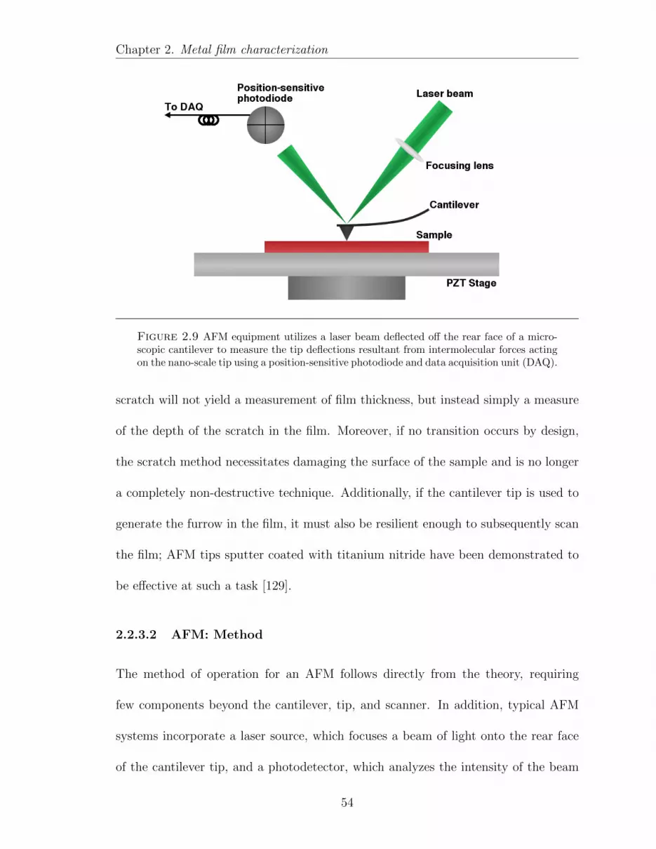
Chapter 2. Metal film characterization
Figure 2.9 AFM equipment utilizes a laser beam deflected off the rear face of a micro-scopic cantilever to measure the tip deflections resultant from intermolecular forces actingon the nano-scale tip using a position-sensitive photodiode and data acquisition unit (DAQ).
scratch will not yield a measurement of film thickness, but instead simply a measure
of the depth of the scratch in the film. Moreover, if no transition occurs by design,
the scratch method necessitates damaging the surface of the sample and is no longer
a completely non-destructive technique. Additionally, if the cantilever tip is used to
generate the furrow in the film, it must also be resilient enough to subsequently scan
the film; AFM tips sputter coated with titanium nitride have been demonstrated to
be effective at such a task [129].
2.2.3.2 AFM: Method
The method of operation for an AFM follows directly from the theory, requiring
few components beyond the cantilever, tip, and scanner. In addition, typical AFM
systems incorporate a laser source, which focuses a beam of light onto the rear face
of the cantilever tip, and a photodetector, which analyzes the intensity of the beam
54

Chapter 2. Metal film characterization
reflected off the tip, as shown in Fig. 2.9. The apparatus may also include a voltmeter
or an arbitrary waveform generator in order to either measure the oscillation of the
cantilever or drive the oscillation with an applied waveform.
The AFM system may be operated in contact mode, wherein the tip remains
in contact with the sample surface throughout testing, or tapping mode, wherein
the spring-like undulation of the cantilever tip is used to measure surface properties
based on attractive and repulsive forces. Furthermore, the apparatus may be de-
signed such that the piezoelectric translational stage (PZT) moves the sample stage
with respect to a fixed cantilever setup, or such that the cantilever and laser setup is
moved with respect to a fixed sample stage; however, both orientations may produce
comparable results. It should be noted that hysteresis in the piezoelectrics may lead
to measurement artifacts and non-linear, inconsistent lateral resolution. However, for
the purposes of film thickness characterization, as long as there is sufficient resolu-
tion at the transition between film and substrate, the thickness should be accurately
measured. Additionally, if the cantilever tip is in motion across the surface, it is rec-
ommended to operate in contact mode to avoid the addition of any vibrations from
the scanning action [114].
2.2.3.3 AFM: Analysis
AFM analysis is much more straightforward than other techniques mentioned herein,
since the reflected laser intensity directly corresponds to the position of the tip relative
to the surface, assuming the system has been properly calibrated. Although only a
single pass over the transition between film and substrate is necessary to measure
55

Chapter 2. Metal film characterization
Figure 2.10 An AFM cantilever tip was used to scratch a furrow in a 14-bilayer polymer-
polyelectrolyte film on a silicon substrate. Cross-sectional analysis revealed the depth of
the furrow, and therefore the thickness of the film, to be approximately 54 nm. [Reprintedfrom Nanotechnology, 14, R. Lobo, et al. , “In situ thickness measurements ofultra-thin multilayer polymer films by atomic force microscopy”, Page 392, Copy-right (1999), with permission from IOP Publishing]
depth, typically a full two-dimensional scan will be performed in order to generate
a three-dimensional surface profile, such as that shown in Fig. 2.10. Scanning over
a large area also ensures that variations, artifacts, and debris on the film surface do
not distort thickness measurements.
Film analysis in such a manner will not only reveal the thickness of the film,
but also aspects of the transition area like steepness and film homogeneity. For
example, the study that recorded the AFM image shown in Fig. 2.10 also noted that
in the course of scratching the furrow in the polymer film, the cantilever tip created
ridges along one edge where the polymer had been pushed to one side. In order to
compensate and accurately determine the thickness of the film, they scanned over a
relatively large area (2500 µm2), so that the baseline used as a top surface reference
would not be distorted by the ridge height.
By scanning the cantilever tip across the furrow, the researchers were able to
56

Chapter 2. Metal film characterization
generate the cross-sectional profile shown in Fig. 2.10, which determined the thickness
of the 14-bilayer film to be approximately 54 nm. Although the specific value is not
quoted in the text, a graph of the number of bilayers plotted against the film thickness
recorded by AFM was presented in the text, which demonstrated a linear relationship
between the two. That said, typical AFM systems have a sub-nanometer vertical
resolution, so as long as the transition between the substrate and the film surface
is being observed, the thickness should be readily determined with a relatively low
degree of error. It should also be noted that such measurements using a furrow to
measure thickness will be fundamentally limited by the sharpness of the cantilever
tip. Moreover, although AFM can indirectly measure the thickness of a thin film
on a substrate without the need for complex curve-fitting, the technique provides
little other information beyond thickness and homogeneity. Consequently, in relating
optical transmission to metal film thickness, AFM is only capable of completing half
of the analysis and so must be used in conjunction with an optically based technique
in order to complete the analysis.
2.2.4 Electron Beam Techniques
Electron beam based technologies represent a categorically different alternative
to traditional techniques that rely on electromagnetic radiation to interrogate sample
surfaces. Although there are a number of different techniques that have spawned from
e-beam approaches, including Auger Electron Spectroscopy (AES) and Transmission
Electron Microscopy (TEM), two technologies have demonstrated particular applica-
tion in determining thin film thickness: cross-sectional Scanning Electron Microscopy
57
Chapter 2. Metal film characterization
(SEM) and Energy Dispersive X-ray Spectroscopy (EDS or EDX). The former tech-
nique uses secondary generated electrons to computationally produce a two dimen-
sional image of a film cross-section, which may provide a clear depiction of the film
sitting atop the underlying substrate layer. By contrast, the latter technique uses
X-rays generated by the incident e-beam to characterize the elemental composition
of the film, which may be compared to the elemental composition of the substrate to
computationally determine the film thickness.
2.2.4.1 E-Beam Techniques: Theory
Both of the techniques mentioned may be performed using an SEM system, although
the SEM-EDS necessitates a suitable X-ray detector in addition to the standard sec-
ondary electron detector used in SEM image generation. In both cross-sectional SEM
and SEM/EDS analysis, a beam of electrons is directed in a column incident upon
the sample surface, generating a variety of effects that are strongly correlated with
the energy of the e-beam, each of which provide an array of information about the
sample and can be utilized to determine a variety of its characteristics. For example,
backscattered electrons may be used to determine sample crystallography; whereas
Auger electrons may be detected to provide information about the surface compo-
sition. Figure 2.11 depicts the characteristically bulbous electron beam interaction
volume and demonstrates the various depths at which each effect is generated.
However, cross-sectional SEM analysis is principally concerned with the topog-
raphy of the film cross-section, and so utilizes the detection of secondary electrons
generated within the sample through inelastic scattering. Although these electrons
58

Chapter 2. Metal film characterization
Figure 2.11 The interaction volume of an incident beam of electrons produces a varietyof effects at different depths. SEM utilizes the secondary 2´ electrons for surface imagingwhereas EDS utilizes characteristic x-rays for elemental analysis
.
bear no significant dependence upon the composition of the region of their origin,
they are highly sensitive to topographical features [130]. Consequently, these elec-
trons are used to generate the traditional tomographical SEM images, which have
become so prevalent in scientific literature, and are widely used in observing and
characterizing thin film surface homogeneity [131]. The lateral resolution of such im-
ages is largely dependent upon the incident beam diameter, which may be as small as
10 A, yielding surface tomographical images with resolutions well beyond the optical
diffraction limit. The typical resolution of standard SEM is included in Table 2.2,
along with the resolutions, limitations, and sample requirements of other standard
materials characterization methods.
59

Chapter 2. Metal film characterization
Additionally, although the properties of the electrons themselves are not re-
lated to sample composition, the likelihood of their generation is dependent upon
the composition of the sample from which they originate, which produces a degree
of contrast between surfaces of differing composition, such as a metal film and its
glass substrate. Moreover, by increasing the tilt angle of the sample, it is possible
to increase secondary electron generation and thereby increase the contrast. Images
produced that demonstrate a discernible difference between the two surfaces are then
analyzed to produce an estimation of the film thickness.
SEM-EDS, on the other hand, relies on X-rays produced through the interaction
of the incident electron beam upon the sample surface [132]. The high energy electrons
bombard the sample and eject secondary electrons from the atomic orbitals. The
ejection of said electrons leaves vacancies in the electron shell, which are filled by
electrons in higher shells. When an electron drops down to fill the vacancy, an X-ray
is produced, whose energy and wavelength are characteristic of the orbital from which
it was generated, and therefore are characteristic of the atom as well. However, not
all X-rays produced through this method are characteristic of the elements they are
generated by. The incident electrons can interact with any electrons in the atomic
orbitals, which can generate a spectrum of other X-rays of differing energies [105].
Nevertheless, the characteristic X-rays may be used to perform chemical analysis
of the sample surface, which may be compared to the chemical composition of the
substrate to determine the relative amount of each element in the film. Although not
an absolute measure of elemental concentration, ratios of the relative amounts of the
elements of interest may be generated to infer film characteristics or to compare the
60

Chapter 2. Metal film characterization
sample to other similar samples for differentiation purposes [133, 134].
2.2.4.2 E-Beam Techniques: Method
The electron beam may be generated through one of two different means: field emis-
sion or thermionic emission. In the former method, electrons are generated by placing
a pointed cold cathode filament in a high potential electric field, which rips electrons
away from the filament and directs them toward the sample. In the latter method,
a strong current is passed through a conducting filament, which generates a beam of
electrons that are directed toward the sample surface. However, the method of gen-
eration is a design parameter of the equipment, rather than an analytical variable.
That being said, regardless of the method of generation, the electron beam must be
created under a high vacuum in order to collimate the beam and prevent premature
electron scattering.
The beam is directed toward the sample through a column of electromagnetic
“lenses”, which collimate, condense, and focus the beam upon the sample surface, as
shown in Fig. 2.12. In addition to these lenses, a pair of scanning coils deflects the
beam so that it may be raster scanned across the surface, so as to generate a two-
dimensional image or analyze a specific section of the sample. The SEM equipment
may also incorporate detectors for each of the aforementioned phenomena; however,
cross-sectional SEM generally utilizes only the secondary electron detector, whereas
SEM-EDS uses both that and the X-ray detector for elemental analysis. In order
to avoid artifacts caused by sample charging, operating the SEM at lower beam
energies around 1.5 kV or less can yield operating resolutions around 1 nm, although
61

Chapter 2. Metal film characterization
Figure 2.12 SEM systems are operated under ultra-high vacuum to minimize electrondiffraction and allow the condenser “lenses” to collimate the electron beam. The samplechamber is equipped with as many different detectors as is necessary, but SEM imaging isperformed using the secondary 2´ electron detector.
insulating samples like the glass or ceramic substrates used in optics should still be
properly grounded [135].
Cross-sectional SEM analysis is functionally identical to traditional SEM in
that a beam of electrons is directed toward the surface of a sample thin film-coated
material. The principal difference is that the cross-sectional analysis necessitates that
the region of interest be either the boarder of a thin film where the full thickness of
the film atop the substrate can be observed, or else is a surface created by cutting
the sample to produce such a cross-section. In the event that an observable border is
present by design, the procedure is non-destructive in nature; however, should there
62

Chapter 2. Metal film characterization
be no such facet, this technique may necessitate damaging the sample.
By contrast, SEM-EDS focuses the incident e-beam onto a sample spot that
is analyzed for a set amount of time, typically around 100 s, so that the electrons
can interact with each element of the sample and under interrogation. Although
EDS can be achieved using any e-beam system, the combination of EDS with SEM
allows for the secondary electron imaging to be utilized as a targeting system. The
SEM generates a two dimensional image of an area of the sample, from which a
point or series of points are selected for interrogation. Analysis of more points allows
for statistical verification of film thickness, given that inhomogeneities may result in
slight variations in thickness calculations.
2.2.4.3 E-Beam Techniques: Cross-Sectional SEM Analysis
With regard to thin film thickness measurement, cross-sectional SEM analysis is per-
formed using image processing software, provided that an appropriate cross-section of
the film and substrate layers has been recorded such that each layer is distinguishable
from the others. Certain manufacturers include image processing as a tool incorpo-
rated into the equipment’s operational software; however, there are also a number of
third party applications that perform the same tasks, including ImageJ, Gimp, and
Adobe Photoshop, assuming that a relevant scale has been included in the image. By
comparing the height of the thin film in pixels over the length of the image to the
scale provided by the SEM software, it is possible to calculate the thickness of the film
in nanometers. The software may also need to take into account the magnification
and the tilt angle of the mount in order to obtain an accurate reading, which may
63

Chapter 2. Metal film characterization
Figure 2.13 Software analysis of the SEM cross-section image reported in Sharp et al.
reveals that the thickness of the Au film is 60.1 nm with a 123.5 nm thick Ni film underneath
on a Si substrate, both with a claimed resolution less than 1 nm; although that resolution
may vary depending upon the degree of contrast between subsequent layers. [Reprintedfrom Microscopy and Microanalysis, 14, S. Sharp, et al. , “Thin film proper-ties measurement using SEM-based energy dispersive spectroscopy for nanosciencestudies”, Page 337, Copyright (2008), with permission from Cambridge UniversityPress]
compound error and result in detrimental effects on the resolution of the technique
depending on the accuracy of the mounting angle measurement.
The SEM image shown in Fig. 2.13 demonstrates an example of a two-film
system deposited on a silicon substrate [102]. The system under interrogation consists
of a thin gold film deposited over a nickel film adhered to the surface of the silicon
substrate, each of which is clearly distinguishable due to the distinct difference in
contrast presented by each material. The image was analyzed using the LayerProbe
64

Chapter 2. Metal film characterization
software and yielded thicknesses of 60.1 nm for the gold film and 123.5 nm for the
nickel film. The paper also reported that measurements had been recorded for the
same system using X-Ray Fluorescence (XRF), yielding thickness values of 61 nm
and 141 nm respectively. Moreover, the software claims that the resolution for each
measurement is 0.7 nm for this analysis, although in other cases error was as low
as 0.1 nm; whereas the resolution of XRF measurements was only 25 nm and 24 nm
respectively [102].
These values suggest that SEM image analysis can provide an extremely ac-
curate measurement of film thickness; however, the situation presented is an ideal
example wherein the films are easily distinguished and there does not appear to be
any blatant image aberration. Under less-than-ideal situations, the measurement
resolution is quickly compromised due to confounding factors such as image aberra-
tions, distortion, lack of contrast, and charge build-up. Moreover, the facet chosen
for analysis may not be representative of the entire surface, so obtaining an accurate
thickness measurement may necessitate the destruction of the sample such that ad-
ditional cross-sections may be imaged. Whereas other methods of analysis may non-
destructively analyze different portions of the film, whether through raster-scanning
the sample surface or independently changing the investigated area, cross-sectional
SEM reveals only information about the observable face. In cases where the sample
is inhomogeneously deposited, cross-sectional SEM may yield in inaccurate or mis-
leading measurement. Consequently, SEM analysis is often used to visually present
the film geometry and thereby gain an estimation of its thickness and surface rough-
ness, but is typically used in conjunction with another analytical method for a more
65

Chapter 2. Metal film characterization
Figure 2.14 EDS analysis yields an X-ray spectrum, with characteristic peaks for eachelement present. Comparing peak ratios of reliable elements, like Si, to the elements ofthe thin film, Ag and Ti, it is possible to calculate film thickness using spectrum analyzersoftware developed at the National Institute of Standards and Technology (NIST).
accurate empirical measure.
2.2.4.4 E-Beam Techniques: SEM-EDS Analysis
In performing SEM-EDS analysis of a sample thin film deposited on a given substrate,
the SEM imaging system is utilized as a targeting system so that the regions of interest
can be identified by the user and interrogated by the e-beam. Each element yields
characteristic X-rays resultant from electron interactions with electrons in the core
atomic orbitals, allowing for the recording of an X-ray energy spectrum, which depicts
the relative presence of each element based on the amplitude of recorded X-rays by
their characteristic energy. In order to accurately record ultra-thin films of elements
with high characteristic X-ray energies, a high speed silicon drift detector is necessary,
due to the need to process counts at a sufficient rate to record the shorter wavelength
X-rays.
Chininis et al. utilized an SEM equipped with a Bruker Quantax 200 Silicon
Drift Detector with Xflash6 to interrogate samples of titanium and silver deposited
66

Chapter 2. Metal film characterization
on silicon glass substrates in order to determine the respective deposition rates of
the two metals in a cold sputter vacuum deposition system [83]. The X-ray energy
spectrum recorded for each sample was utilized to compare the peak amplitude of
the silicon peak to that of the element being analyzed, as shown in Fig. 2.14. Silicon
was used due to its stability within the glass chemistry, allowing for the recording of
reliable Counts Per Second by electron-volt (cps/eV) for each of the relevant elements
in the sample.
Following that, elemental ratios of silicon to the element of interest (either silver
or titanium) were generated and the NIST DTSA-II (National Institute of Standards
and Technology Desktop Spectrum Analyzer-II) software was used to produce a simu-
lation of experimental conditions, while iteratively varying film thickness on a homoge-
nous substrate in order to compare the recorded elemental ratios to those predicted
though simulations. The ratios of silicon/titanium and silicon/silver were calculated
for each simulation, varying film thickness until the ratios matched the recorded data,
allowing for the determination of film thickness by comparing recorded measurements
to the theoretically predicted models. The authors were able to calculate thickness
measurements in such a manner and determine the titanium deposition rate to be
0.10 nm/s and the silver deposition rate to be 1.19 nm/s. Consequently, provided the
SEM is equipped with an appropriate X-ray detector, it may be possible to perform
calculations to determine the film thickness by comparing measured values to DSTA
software simulations based on NIST data.
67

Chapter 2. Metal film characterization
2.3 Characterization limitations & considerations
The techniques discussed herein are some of the more useful methods of charac-
terizing metal thin films. However, there are myriad other modalities for characteriz-
ing thin films, many of which are listed in Table 2.2. Each of these technologies has its
benefits, but many are poorly suited to characterizing metal thin films in particular.
Some of the more common limitations are included in the sections to follow, along
with some useful considerations for the interested reader.
2.3.1 Radiative absorption
Many of the techniques mentioned herein and included in Table 2.2 are based on
some form of photon propagation, whether within the X-ray, UV, Visible, or Infrared
spectra. Consequently, these methods are subject to the influence of the optical prop-
erties of the samples in question, such as their absorption and scattering coefficients.
This work focuses on metal films, which samples are largely reflective, particularly at
greater thicknesses; however, they also tend to have a non-zero absorption coefficient,
which is incorporated as part of the complex refractive index n = n+ iκ, where n is
the real portion of the refractive index, which governs the relative speed of light in
the medium, and κ is the imaginary component, which governs optical absorption.
The complex refractive index, and therefore the absorption of photons, may
have a profoundly negative effect on the efficacy of any radiative technique, particu-
larly techniques like XRR and ellipsometry, which rely heavily upon specific changes
resultant from the incident beam partially reflecting off the front and rear faces of
68
Chapter 2. Metal film characterization
the sample at each film interface. The greater the absorption within the film, the
less accurate the measured change will be. This is particularly true for thicker films,
wherein significant absorption reduces the effective mean free path of the photons
passing through the film, which consequently decreases the number of photons that
are able to escape the medium and therefore the intensity of the detected beam. This
effect may alter the amplitude of the reflected intensity profile and skew the data
away from the true values of film thickness, which can have a compounding effect for
techniques that rely on computational curve fitting for thin film analysis. It is for
this reason that many thin film characterization companies state that their software
is only reliable for metal films between 0.5–50 nm thick, beyond which regimes the
software can no longer accurately match the model to the data in a reliable fashion;
although custom-built laboratory equipment may be able to out-perform commer-
cially available equipment. Figure 2.5 is a principal example of such limitations, as
the data for the thicker films is less defined and resulted in a poorer parameterized
fit. The margin of error in the fit resulted in a slightly worsened resolution as well.
It is advisable, therefore, that the radiative absorption spectrum of the elements that
comprise the sample be considered when selecting a radiative technique, given that
metals may be highly absorbing in the one spectral regime, but largely transmissive
in another.
2.3.2 Sample conductivity
Another significant category of techniques utilized in thin film characteriza-
tion involves the use of electron beams, as are used in SEM and Auger Electron
69

Chapter 2. Metal film characterization
Spectroscopy (AES), beams of charged ions, as used in Medium Energy Ion Scat-
tering (MEIS), or electrical current, as employed in Scanning Tunneling Microscopy
(STM). As a result, all such techniques are subject to the likelihood for charge build-
up on the sample surface if not appropriately grounded, which can have substantial
consequences for both the resolution of the technique and the serviceability of the
equipment.
This work focuses on metal films in optical applications, which frequently in-
volve film deposition onto optically transparent, but electrically insulating substrates.
That being the case, electrical charge build-up is a strong possibility. Techniques like
SEM, which rely on the detection of electrons ejected from the sample utilize incredi-
bly sensitive equipment designed to detect small amounts of electrons. Consequently,
an charge build-up may permanently damage the detector/analyzer, but will almost
certainly “white-wash” the SEM image, thereby disrupting the necessary contrast for
discerning film layers, deteriorating the spatial resolution of the image, and render-
ing any desired tomographical profile unreliable. Operating at a lower vacuum and
reintroducing gases into the SEM may improve contrast and allow for charge to be
conducted away from the sample surface, but also introduces a greater likelihood for
e-beam interaction with the gas in the form of diffraction or scattering, which can
have a negative influence on spatial resolution.
Moreover, techniques that employ X-ray radiation may also suffer from charge-
related problems as X-rays of such a wavelength as to be capable of interacting with
the valence electrons in metal films and thereby elevating them to a higher energy
state or otherwise ejecting them away from the film surface entirely. In the case of
70

Chapter 2. Metal film characterization
XRR, the charge build-up may damage the equipment as it discharges to other com-
ponents, but may also affect the intensity of the specularly reflected beam. The use
of conductive adhesive, such as copper tape, to form an electrical connection between
the film layer and the sample stage may mitigate charge build-up concerns, but may
have undesirable consequences on the adhesion regions of the sample, undermining
otherwise non-destructive techniques.
2.3.3 Derived vs. measured thickness
Although Table 2.2 lists a number of other limitations and considerations, per-
haps the most important consideration to bear in mind is the difference between
computationally derived film thickness values, such as are provided by techniques like
UV-Vis Spectrophotometry, XRR, and Ellipsometry, and thickness values directly
correlated to an empirical measurement, as are provided by techniques like STM and
AFM. The latter variety are typically contact-based technologies that often offer sub-
nanometer depth resolutions and extremely reliable measurements owing to the use of
vibration-damping systems to mitigate noise and error; however, they also necessitate
transition regions on the samples to provide vertical contrast between substrate and
film layers, and as such are limited either to only those samples that incorporate such
regions, or those samples that allow for destructive testing conditions.
When such conditions are not met, the former variety of techniques are prefer-
able, typically guaranteeing non-destructive testing and nano-scale resolutions. How-
ever, such methods rely on computational modeling or curve fitting to derive film
characteristics, and as such are only as accurate as the margin of error for the mod-
71

Chapter 2. Metal film characterization
els. Consequently, the parameters of the model, such as refractive index and film
thickness, may place limitations on the reliability of the measurement, as the er-
ror residuals increase. Figure 2.5 again provides an example wherein the analysis of
thicker films exhibited greater error in the model fit and a correspondingly worsened
depth resolution. As a result, derived thickness values are subject to computational
error, inaccuracies of fit, and potentially substantial deviations away from the the-
oretically expected model. Moreover, when making use of any such computational
techniques, it is essential that the operator also be aware of the theoretical assump-
tions upon which the software is operating. Moreover, said assumptions will likely
change based on the various types of models and statistical analyses available in the
software.
2.4 Conclusions and developing technologies
Due to their reflectivity and optical absorption, metal thin films often provide
a challenge for many of the most predominant characterization techniques available.
Of the methods covered in this review, AFM provides the most accurate and reliable
measure of film thickness, with a potentially sub-Angstrom resolution, although it
provides little other information and places certain requirements on the samples.
Following that, SEM/EDS offers both an image of the film surface, which may grant
information about the surface homogeneity, along with a computationally derived film
thickness and elemental composition spectrum. The resolution is not quite on par with
AFM, but for the purposes of film analysis in optics and biophotonics, it is sufficient,
given that the technique can analyze films regardless of their optical reflectivity or
72

Chapter 2. Metal film characterization
absorption while still offering an optically relevant thickness measurement.
On the other hand, the other techniques, both based on radiative measurements,
demonstrate varying efficacy and are highly dependent upon the film thickness, ab-
sorption, and refractive index. Ellipsometry is reportedly limited to metal films less
than 50 nm thick, whereas XRR can reliably double that limit, although the degree
of error in thickness value grows as thickness increases. In contrast to the other tech-
niques, cross-sectional SEM does not actually provide a thickness value. However,
image analysis can afford the observer with an idea of the overall thickness and the
homogeneity of the film over a broad surface area. That said, it only provides local
thickness characteristics at the cross section, and therefore would necessitate that the
sample be fractured into multiple pieces to generate more cross-sections to analyze
for statistical reliability.
Consequently, it is the opinion of the authors that if the refractive index of
the metal film is of little to no consequence, contact based profilometry techniques
like AFM offer the most reliable measurement of thickness alone. In the event that
a transition region is not incorporated nor destructive testing methods permissible,
SEM/EDS is a suitable alternative technique, if available. Nevertheless, each of
the other techniques, particularly XRR, can provide reasonably accurate estimations
through their derivations; however, investigators should be aware of the operational
limitations of the techniques. It is recommended that should AFM or SEM/EDS
not be a viable option, a reliable measure of thickness may be obtained through the
combination of a radiative technique with cross-sectional SEM. Moreover, should the
optical properties of the film be unknown and desired, employing additional thickness
73

Chapter 2. Metal film characterization
characterization techniques as confirmation can add reliability to radiative methods
whose derivations may depend on geometric and optical parameters.
Having introduced some of the more predominant characterization methods and
included a table of potentially viable alternatives that have seen some use in liter-
ature, it is worth noting that there are also new techniques in development for the
characterization of thin films. One such technique, Total Internal Reflection Pho-
toacoustic Spectroscopy (TIRPAS), falls into the category of Evanescent Field-based
Photoacoustics (EFPA), and has been demonstrated in the characterization of the
thickness and refractive index of optically transparent thin films [136]. Variations
of the same technology have been suggested for use with metal and other optically
absorptive thin films, in the form of Surface Plasmon Resonance Photoacoustic Spec-
troscopy (SPRPAS) and Optical Tunneling Photoacoustic Spectroscopy (OTPAS), in
addition to applications involving the detection of absorbing particles [106, 137].
EFPA techniques utilize the same evanescent field depicted in Fig. 2.2, but with
the intention of generating acoustic pulses following the absorption of the field’s opti-
cal energy. In such applications, a sufficiently short laser pulse (less than 1µs) totally
internally reflects within a prism or waveguide, thereby generating an evanescent field
within the external medium, which is typically the sample thin film. The portion of
the field that penetrates through the film may be absorbed by chromophores in the
medium beyond the film, which in turn incites an ultrasonic pressure wave through
the optical absorption and resultant rapid thermoelastic expansion of the absorber.
This acoustic energy may then be detected by a suitable ultrasonic transducer, which
yields information about the film’s optical and geometric properties, including re-
74

Chapter 2. Metal film characterization
fractive index and thickness [138]. The peak-to-peak magnitude of the photoacoustic
pressure wave is directly related to the film thickness, its refractive index, and the in-
cident angle of the laser beam. Consequently, by scanning through a range of incident
angles, it is possible to determine the critical angle of the film-prism interface, calcu-
late the refractive index using Snell’s Law based on the known refractive index of the
prism, and thereafter derive the film’s thickness. Although this method has similar
limitations to the other aforementioned optical approaches, the range of detectable
film thicknesses is theoretically directly related to the wavelength of the incident light.
Consequently, for thicker films, a longer wavelength should ideally provide accurate
results, whereas for thinner films, a shorter wavelength may prove more effective.
Nevertheless, considering the recent breakthroughs in thin film chemistry, film
deposition techniques, and meta-material fabrication, along with the continuous stream
of new optical thin film applications being envisioned each year, the accurate depth
profiling of thin films on insulating substrates represents a critical milestone in the
advancement optical technologies. This is particularly the case for technologies akin
to the waveguides discussed in Section 2.1.1, which rely on sub-wavelength electro-
magnetic effects, such as evanescent field interactions and surface plasmon resonance,
to achieve what macroscale techniques could not. As such, whether it is a new concep-
tual modality still being substantiated or an established technique being iteratively
improved, the further advancement of both noted and novel thin film characteriza-
tion technologies is anticipated to play a significant role in the future of optics and
biophotonics.
75

Chapter 3
Selective release waveguides andcontact-based laser irradiation of tissue
Portions of this chapter have been reproduced with permission from the Master’s
Thesis entitled Photonic Ablation via Quantum Tunneling, authored by Paul J.D.
Whiteside, Bioengineering Department, University of Missouri, May (2015) [1].
3.1 Introduction
Whereas the previous chapters first presented a background in medical bio-
photonics and the applications of light-based procedures therein followed by a com-
prehensive overview of metal thin film applications and the most appropriate and
effective characterization techniques, the following sections discuss the concept of
the planar “selective-release waveguide” (SRW), the principal innovation that forms
the foundation of this dissertation and permits the incorporation of secondary tech-
nologies without necessitating their alteration or compromising their efficacy. As a
brief overview, the SRW technique involves the fabrication of a planar optical waveg-
uide through which laser light may be transmitted. Such waveguides are designed
to transmit light through designated “active areas” on one of their largest facets. In
76

Chapter 3. Selective-release design
biophotonics applications, upon direct contact of the waveguide’s active area with a
tissue or tissue-like medium, the light within the SRW substrate either refracts or
optically tunnels out of the waveguide into the external medium. Furthermore, by
tuning the composition and thickness of the active area materials, it is possible to
regulate the portion of light that is transmitted out of the waveguide at each in-
ternal reflection point. The following sections discuss the technical aspects of this
transmission approach in greater detail, along with a subsequent description of the
experimental methods employed to establish the technique and quantify the trans-
mission of pulsed light into ex vivo porcine tissue samples using planar, metal-clad
SRW’s of differing active area film thicknesses.
3.2 Technical discussion
The cardinal strength of the selective release waveguide technology lies in its
foundation upon well-established optical principles, the most fundamental of which
is the concept of the optical waveguide (a.k.a. “lightguide”). Such materials are
utilized to transmit or redirect electromagnetic waves in the Ultraviolet (UV), Visible,
and Near-Infrared (N-IR) spectra. Waveguides composed of optically transparent
materials function by reflecting light within their bounding surfaces, forcing the light
to propagate along their length [92, 139]. This section provides a mathematical
description for waveguide operation starting with optical first principles established
by the likes of Isaac Newton, James Clerk Maxwell, and Augustin-Jean Fresnel.
77

Chapter 3. Selective-release design
3.2.1 Operating conditions of planar optical waveguides
Optical waveguides have been used extensively in a variety of applications, in-
cluding optoelectronic integrated circuitry, attenuated total reflection spectroscopy
(ATR), and laser beam generation within planar waveguides; however, our appli-
cation is intended for use in the controlled delivery of light into tissue and for that
endeavor we must consider the types of interactions light can undergo along the length
of the waveguides in question [69–71].
3.2.1.1 Maxwell’s and Fresnel’s Equations
With regard to the operation of optical waveguides, when considering the propagation
of light within the waveguide substrate, the optical properties of both the substrate
and cladding materials collectively determine the behavior of any beam of photons
incident upon their interface. Such a beam may either refract into the external
medium, travel along the interface, or totally internally reflect back into the substrate,
dependent upon the relative refractive indices of the two media and the angle of the
incident beam with respect to the interface. Waveguide operation demands that the
light within the substrate repeatedly totally internally reflect at each interface, until
reaching a designated exit aperture. The mathematical equations that govern each of
these conditions are collectively known as the Fresnel Equations, and can be directly
78

Chapter 3. Selective-release design
derived from Maxwell’s Equations in isotropic media, shown below [140].
∇×H = j +∂D
∂t(3.1)
∇×E = −∂B∂t
(3.2)
∇ ·D = ρ (3.3)
∇ ·B = 0 (3.4)
j = σE (3.5)
D = εE (3.6)
B = µH (3.7)
Expressing the Wave Equation in terms of only the Electric Field, E, necessitates
that the magnetic components of Maxwell’s Equations (H and B) be replaced with
their electric equivalents. Combining and reducing Maxwell’s Equations to only their
electric components yields the Laplacian of E, shown below in Eq. (3.8).
∇2E = µσ∂E
∂t+ µσ
∂2E
∂t2(3.8)
One solution of this equation is in the complex form of a plane-polarized har-
monic plane wave:
E = E exp[iω(t− x
v
)](3.9)
with the condition that:ω2
v2= ω2εµ− iωµσ (3.10)
79

Chapter 3. Selective-release design
In this representation, E represents the vector amplitude for the Electric wave.
The complex representation of the refractive index (n = n− iκ) can then be readily
derived from Eq. (3.10) by defining n2 = c2
v2. This representation utilizes n and κ to
represent the real and complex components of the refractive index respectively. By
accounting for the speed of light (c), relative permeability (µr), relative permittivity
(εr), and the complex refractive index, Equation (3.9) can be rewritten to incorporate
some of the more useful optical properties. The equation can then be generalized for
any plane-polarized wave propagating in the direction given by the unit vector s =
〈αi+ βj + γk〉, to yield the Wave Equation in terms of E in Eq. (3.11). Additionally,
a more rigorous derivation is included in Appendix A.
E = E exp
[i
(ωt−
(2πn
λ
)(αx+ βj + γz)
)](3.11)
By a similar process, it is also possible to derive the Wave Equation in terms of
only its magnetic components, yielding Eq. (3.12) below.
H = H exp
[i
(ωt−
(2πn
λ
)(αx+ βj + γz)
)](3.12)
Whereas polarization does not have any implications for a beam that is normal
to the interface, since the magnetic and electric components would both be parallel
to the interface, in cases of oblique incidence in non-absorbing media, as is observed
in optical waveguides, the polarization state of the beam has distinct implications
with regard to the relative reflection and transmission coefficients. For the purposes
80

Chapter 3. Selective-release design
Figure 3.1 The sign conventions defining the positive directions for the Electric andMagnetic components of an obliquely incident beam upon a secondary medium for [left]Transverse Magnetic (TM, p-) polarized light and [right] Transverse Electric (TE, s-)polarized light.
of this study, we will consider the case of a beam that is linearly polarized with a
transversely electric component. This polarization state is referred to as TE or s-
polarized, wherein “s” stands for “senkrecht” (German for “perpendicular”). The
alternative polarization state is that of the transverse magnetic beam, referred to as
TM or p-polarized, wherein “p” stands for “parallel” (the derivation for the transverse
magnetic component is included in Appendix A).
The positive sign conventions for both polarizations of an obliquely incident
beam are shown in Figure 3.1, with the conventions for TM polarized light on the
[left] whereas those for TE polarized light are on the [right]. Based on these con-
ventions, the boundary conditions for an obliquely incident s-polarized beam are
mathematically represented below:
81

Chapter 3. Selective-release design
Ei + Er = Et (3.13)
Hi cosϑ0 −Hr cosϑ0 = Ht cosϑ1 (3.14)
Again, we will derive these conditions such that they deal with only the electric
field. It is important to note that the cosϑ terms arise from translating s over to
perpendicular incidence, so that E and H are tangential (parallel) to the surface.
Furthermore, it is convenient to define new variables to represent components of the
translated boundary conditions, as shown below:
Ei = Ei
Er = Er
Et = Et
Hi = Hi cosϑ0 = Y0 cosϑ0Ei
Hr = Y0 cosϑ0Er
Ht = Y1 cosϑ1Et
Rewriting the boundary conditions in the terms shown above yields Eq. (3.15)
and (3.16), from which we can obtain expressions for the amplitude reflection and
transmission coefficients for p-polarized light, ρs and τs in Equations (3.17) and (3.18)
respectively, by defining ρs = ErEi
and τs = EtEi
. In this form, Y represents the optical
admittance in non-absorbing media equivalent to Y = nY = n√
ε0µ0
, where Y is the
characteristic optical admittance of free space.
82

Chapter 3. Selective-release design
Hi − Hr = Ht (3.15)
Y0 cosϑ0Ei − Y0 cosϑ0Er = Y1 cosϑ1Et (3.16)
= Y1 cosϑ1 (Ei + Er) (Sub. in Eq. 3.13)
Ei (Y0 cosϑ0 − Y1 cosϑ1) = Er (Y0 cosϑ0 + Y1 cosϑ1) (Distribute and factor)
Er
Ei
=Y0 cosϑ0 − Y1 cosϑ1
Y cosϑ0 + Y cosϑ1
(Rearrange fractions)
ρs =Er
Ei
(Definition of ρ)
∴ ρs =Y0 cosϑ0 − Y1 cosϑ1
Y cosϑ0 + Y cosϑ1
(3.17)
Y0 cosϑ0Ei − Y0 cosϑ0Er = Y1 cosϑ1Et (Continued from above)
Y0 cosϑ0Ei − Y0 cosϑ0 (Et − Ei) = Y1 cosϑ1Et (Sub in Eq. 3.13)
Ei (2Y0 cosϑ0) = Et (Y0 cosϑ0 + Y1 cosϑ1) (Factor)
Et
Ei
=2Y0 cosϑ0
Y0 cosϑ0 + Y1 cosϑ1
(Divide by Ei)
τs =Et
Ei
(Definition of τ)
∴ τs =2Y0 cosϑ0
Y0 cosϑ0 + Y1 cosϑ1
(3.18)
Next we define the expressions for the Irradiance of each of the three beams of
interest, wherein Ii represents the Irradiance of the incident beam derived from the
general expression for Irradiance, as shown below.
83

Chapter 3. Selective-release design
I =1
2R E ×H∗ (3.19)
I = R
1
2E (Y cosϑE)∗
(Scalar Irradiance)
∴ Ii =1
2Y0 cosϑ0EiE
∗i (3.20)
Following along the same approach, we will now define Ir and It in terms of Ii
in order to derive the relative reflection and transmission coefficients for s-polarized
light, Rs and Ts respectively.
Ir = R
1
2Er (Y0 cosϑ0Er)
∗
(Scalar Reflected Irrdiance)
=1
2ρsEi (Y0 cosϑ0ρsEi)
∗ (Er = ρsEi)
=1
2ρ2sY0 cosϑ0EiE
∗i (Reflect the format of Ii)
∴ Ir = ρ2sIi (3.21)
It = R
1
2Et (Y1 cosϑ1Et)
∗
(Scalar Transmitted Irradiance)
=1
2τsEi (Y1 cosϑ1τsEi)
∗ (Et = τsEi)
=1
2τ 2sY1 cosϑ1
Y0 cosϑ0Y0 cosϑ0EiE
∗i (Reflect the format of Ii)
∴ It =Y1 cosϑ1
Y0 cosϑ0
τ 2s Ii (3.22)
From here, considering the simple energy balance equation below allows for
the direct derivation of Rs and Ts. It is also worth noting that by translating s
to perpendicular incidence and incorporating the cosϑ components, the traditional
84

Chapter 3. Selective-release design
condition that 1−R = T still holds true.
I0 = I1 (Conservation of energy)
R
1
2E0 ×H∗
0
= R
1
2E1 ×H∗
1
(Sub in. Eq. 3.19)
R
1
2(Ei + Er) (Hi − Hr)
∗
= R
1
2EtH
∗t
(Scalar components)
1
2(Ei + Er) (Y0 cosϑ0Ei − Y0 cosϑ0Er)
∗ =1
2EtY1 cosϑ1E∗t (H = Y cosϑE)
1
2Y0 cosϑ0 (Ei + ρsEi) (Ei − ρsEi)
∗ =1
2Y1 cosϑ1τ
2sEiE
∗i (Er = ρsEi)
1
2Y0 cosϑ0EiE
∗i
(1− ρ2
s
)=
1
2Y1 cosϑ1τ
2sEiE
∗i (Factor)
=1
2Y1 cosϑ1
Y0 cosϑ0Y0 cosϑ0τ
2sEiE
∗i
Ii(1− ρ2
s
)=
1
2Y1 cosϑ1
Y0 cosϑ0
Ii (Sub. in Eq. 3.20)
Ii − ρ2sIi =
1
2Y1 cosϑ1
Y0 cosϑ0
Ii (Distribute)
Ii − Ir = It (Sub in Eq. 3.21, 3.22)
1− IrIi
=ItIi
(Divide by Ii)
∴ 1−R = T (3.23)
Following from this, we find the expressions for Rs and Ts shown below in
Equations (3.24) and (3.25), respectively.
Rs = ρ2s =
(Y0 cosϑ0 − Y1 cosϑ1
Y0 cosϑ0 + Y1 cosϑ1
)2
(3.24)
Ts = τ 2s
(Y1 cosϑ1
Y0 cosϑ0
)=
4Y0Y1 cosϑ0 cosϑ1
(Y0 cosϑ0 + Y1 cosϑ1)2 (3.25)
By substituting Y = nY , the traditional form of the Fresnel equations for s-
polarized light are produced.
85

Chapter 3. Selective-release design
Rs =
(n0 cosϑ0 − n1 cosϑ1
n0 cosϑ0 + n1 cosϑ1
)2
(3.26)
Ts =4n0n1 cosϑ0 cosϑ1
(n0 cosϑ0 + n1 cosϑ1)2 (3.27)
These equations describe the degree of transmission and reflection observed at
the intersections of two materials of differing optical properties, namely the waveguide
and any surrounding material. When a beam of light is incident upon a planar in-
terface, such as those shown in Figure 3.1, a portion of the light may reflect whereas
the remainder may refract into the secondary medium. For each of the preceding
equations, Ts represents the percent of light incident upon the intersection that is
transmitted into the second medium, whereas Rs represents the percent of light re-
flected back within the original material. A similar derivation yields the percent
reflection (Rp) and transmission (Tp) for p-polarized light, shown below in Equations
(3.28) and (3.29) respectively.
Rp =
[n0
cosϑ0− n1
cosϑ1n0
cosϑ0+ n1
cosϑ1
]2
(3.28)
Tp =4n0n1
cosϑ0 cosϑ1(n0
cosϑ0+ n1
cosϑ1
)2 (3.29)
3.2.1.2 Snell’s Law
In cases of refraction, the Fresnel Equations govern the degree of reflection and re-
fraction at the interface, leaving a portion of the incident beam to propagate within
86

Chapter 3. Selective-release design
Figure 3.2 The conditions for the three possible outcomes of the Fresnel equations andSnell’s Law are: (a) when n2 > n1 light is refracted into the second material, (b) when
n2 < n1 and θ = θc the light travels along the intersection, or (c) when n2 < n1 and
θ > θc the light undergoes TIR.
each material. However, there are two additional possible outcomes, wherein there is
no observable refraction and T = 0, as shown in Figure 3.2 (b) and (c). In order to
determine the conditions at which these outcomes occur, we must first derive another
equation to directly relate the refractive indices and propagation angles of each the
incident, transmitted, and reflected beams.
We start by considering the Irradiance of each of the three beams individually.
The general expression for Irradiance can be concisely represented in the following
manner:
I =1
2nY |E|2 exp
[−4πk
λ(αx+ βy + γz)
](3.30)
Following that, we apply a few simple boundary conditions:
87

Chapter 3. Selective-release design
• the tangential components of E and H are continuous across the boundary
• sreflected = 〈αr, βr, γr〉
• stransmitted = 〈αt, βt, γt〉
From these conditions, we can represent each of the three wavefronts of interest –
incident, reflected, and transmitted – consistently for both Electric and Magnetic
components in the following forms:
Incident : exp
[i
(ωit−
(2πn1
λi
)(x sinϑ1 + z cosϑ1)
)]Reflected : exp
[i
(ωrt−
(2πn1
λr
)(αrx+ βry + γrz)
)]Transmitted : exp
[i
(ωtt−
(2πn2
λt
)(αtx+ βty + γtz)
)]
Then, in order to satisfy continuity for all x, y, and t at z = 0, it can be
determined that ωi ≡ ωr ≡ ωt. In other words, there is no change in frequency for
reflected or transmitted waves as compared to the incident wave. That being the
case, we can extend the identical equality to the wavelength, such that λi ≡ λr ≡ λt.
Additionally, since the representation of the incident beam is oriented such that it
is independent of y, the conclusion can be drawn that the directions of the reflected
and transmitted waves are confined to the plane of incidence. The mathematical
implications of these observations are as follows:
88

Chapter 3. Selective-release design
0 ≡ n1βr ≡ n2βt(2πn1
λ
)(x sinϑi + z cosϑi) ≡
(2πn1
λ
)(αrx+ γrz)
≡(
2πn2
λ
)(αtx+ γtz)
∴ sinϑ = α
∴ cosϑ = γ
n1 sinϑi ≡ n1αr ≡ n2αt (3.31)
Following from Eq. 3.31 and defining the angles of reflection and transmission
to be ϑr and ϑt respectively, we find the following relation to be true.
n1 sinϑi ≡ n2αt (From Eq. 3.31)
= n2 sinϑt (3.32)
Redefining ϑi and ϑt to be ϑ1 and ϑ2 respectively, results in the traditional
expression for Snell’s Law shown below:
n1 sinϑ1 = n2 sinϑ2 (3.33)
3.2.1.3 Waveguide operation
In order for a material to operate as a waveguide, the light must be totally internally
reflected within the bounds of the material, such that all of the light incident upon
the intersection of the substrate and external medium reflects back within the original
89

Chapter 3. Selective-release design
medium, as shown in Figure 3.2 (c). Optical waveguides operate exclusively under
this third condition, such that the refractive index of the external medium (n2) is
less than that of the waveguide (n1), forcing the light to internally reflect between
its surfaces as it propagates along the length of the waveguide. However, in order
to achieve total internal reflection (TIR), the incident angle of the light upon the
boundary must also be greater than the critical angle, θc, which can be mathematically
determined from Snell’s Law (eq. 3.33) [93].
n1 sin θ1 = n2 sin θ2 (3.34)
θc = arcsin
(n2
n1
)(3.35)
Assuming that the external material is of lower refractive index than the waveg-
uide, it can be determined that sin θ2 → 1, which reduces Snell’s Law to equation
(3.35), allowing for direct calculation of the critical angle when n1 and n2 are known.
Using this value in conjunction with the Fresnel equations for reflectivity for TE and
TM polarized light (Eq. (3.26) and 3.28 respectively) allows for the generation of
a plot depicting polarization-dependent reflectivity versus internal reflection angle.
For example, the reflectivity for a waveguide composed of BK7 glass (n1 = 1.519)
considering the external material to be air (n2 = 1.0) is shown in Figure 3.3 [72]. The
graph demonstrates that the reflectivity for TE polarized light is consistently greater
than for TM polarized light, until the critical angle at θc = 41.17°, after which the
light undergoes total internal reflection. Additionally, the TM polarization reflectiv-
ity drops to 0 at the Brewster Angle, which is given by Equation (3.36), and is derived
90

Chapter 3. Selective-release design
0 10 20 30 40 50 60 70 80 90
0
0.2
0.4
0.6
0.8
1
Internal Reflection Angle (deg)
Refl
ecti
vity
Reflectivity vs. Internal Reflection Angle by Polarization: Glass–Air
Rp
Rs
1
Figure 3.3 The reflectivity for p-polarized light is consistently lower than for s-polarizedlight, until the critical angle at θc = 41.17°, after which the light undergoes TIR.
in Appendix (A.2.2.4).
θB = tan−1
(n2
n1
)(3.36)
However, in most cases it can not be assumed that only air will come in contact
with the waveguide. Consequently, for most waveguides TIR is ensured by design
through the incorporation of a cladding layer of known refractive index to encap-
sulate the waveguide, as shown in Figure 3.4 [90, 141]. Typically, optical waveg-
uide substrates are composed of transparent polymers, like Poly-methyl methacrylate
(PMMA, n = 1.49), ceramics, or glasses, like Sapphire (n = 1.77) or Borosilicate BK7
glass (n = 1.519) [72, 142]. By selecting one such substrate with known refractive
index, θc can subsequently be scaled by the appropriate selection of the cladding ma-
91

Chapter 3. Selective-release design
Figure 3.4 Light in a waveguide undergoes TIR when n2 < n1 and θ exceeds the criticalangle. This can be ensured by cladding the waveguide in a polymer or reflective metal layerof lower refractive index than the substrate.
terial. For example, using polymer claddings with refractive indices around n = 1.32
on a BK7 glass substrate typically results in a relatively large θc = 60.34°; however,
choosing such a material limits the angles that support TIR to only those between
60.34° and 90°.
On the other hand, certain metal claddings allow for a much broader range
of total internal reflection angles, since they may have substantially lower refractive
indices. For example, the polarization-dependent reflectivity plot for a BK7 glass
waveguide clad in Silver (n = 0.142) is shown in Figure 3.5. The figure shows that
the metal ensures a broad range of angles that support TIR after the critical angle of
5.36°, although the p-polarized light experiences a substantial decrease in reflectivity
until the Brewster Angle at 5.34°. Such metal claddings demonstrate high reflectivity
in the visible spectrum and support TIR throughout a much broader spectrum of
angles; however, they also tend to introduce a degree of optical absorption, which
may result in energy loss over long distances [73].
92

Chapter 3. Selective-release design
0 10 20 30 40 50 60 70 80 90
0
0.2
0.4
0.6
0.8
1
Internal Reflection Angle (deg)
Refl
ecti
vity
Reflectivity vs. Internal Reflection Angle by Polarization: Glass–Silver
Rp
Rs
1
Figure 3.5 Using Silver as a cladding allows for a wide range of acceptable angles thatsupport TIR, from around 5.4 < θ1 < 90°. However, the reflectivity of TM polarized lightis severely limited at angles less than θc.
3.2.2 Evanescent fields and optical tunneling
The following section provides a discussion of the nano-scale effects observed at
the bounding interfaces of an optical waveguide. Whereas the previous explanation
of TIR and waveguide operation provides a conceptual overview of the phenomena
involved in light transmission, the wave nature of light causes a variety of problems
when describing TIR, due to common assumptions resultant from classical mechanics.
In classical mechanics, particularly on the macroscale, light is traditionally
treated as a particle propagating in distinct energy packets referred to as photons. As
such, diagrams like that shown in Figure 3.4 depict the paths of these photons bounc-
ing off the surfaces of the waveguide like particles off a barrier. However, research has
93

Chapter 3. Selective-release design
demonstrated, even as far back as Isaac Newton, that the energy of the photons does
not merely reflect off the surface, but rather exhibits a degree of penetration into the
surrounding material [143].
3.2.2.1 Evanescent fields
By contrast, treating the light as an electromagnetic wave instead of a discrete parti-
cle reveals that upon interacting with a secondary material of lower refractive index,
the energy of the incident wave slightly crosses the interface of the two materials, pen-
etrating the external medium in the form of an exponentially decaying field of energy,
referred to as the evanescent field. In mathematically deriving the existence of the
evanescent field, it is necessary to account for the non-propagating nature of the field
first by defining the “propagation” vector s2 = 〈sin θ2i+ 0j + cos θ2k〉, and second by
recognizing that θ2 technically does not exist, since there is no refracting portion of
the beam. Consequently, in the course of the derivation, all terms containing θ2 will
need to be substituted out for terms that still apply to the situation of total internal
reflection. We will also define E0,2 to be the electric field in the second medium and
E0,2 to be the amplitude of the field of interest. It is also convenient to temporarily
define the wave vector k2 = 2πnλ0
for simpler expressions during the derivation.
94

Chapter 3. Selective-release design
E0,2 = E0,2 exp
[i
(ωt−
(2πn
λ0
)s2 · ~r
)](From Eq. A.15)
= E0,2 exp [i (ωt− k2s2 · ~r)] (Sub. in k2)
= E0,2 exp [i (ωt− k2x sin θ2 − k2z cos θ2)] (Dot product)
= E0,2 exp[i(ωt− k2x sin θ2 ± k2z
(1− sin2 θ2
) 12
)](Trig. substitution)
= E0,2 exp
[i
(ωt− k2x
n1
n2
sin θ1 ± k2z
(1− n2
1
n22
sin2 θ1
) 12
)](Snell’s law)
= E0,2 exp
[i
(ωt− k2x
n1
n2
sin θ1 ±k2
n2
z(n2
2 − n21 sin2 θ1
) 12
)](Factor n2)
= E0,2ei(ωt−k2xn1n2 sin θ1
)e− k2n2z(n2
1 sin2 θ1−n22)
12
(Factor i)
= E0,2ei(ωt− 2πn2n1
λ0n2x sin θ1
)e− 2πn2λ0n2
z(n21 sin2 θ1−n2
2)12
(Sub. out k2)
= E0,2ei(ωt− 2πn1
λ0x sin θ1
)e− 2πλ0z(n2
1 sin2 θ1−n22)
12
(Simplify)
By defining δ to be the penetration depth of the evanescent field into the sec-
ondary (rarer) medium, and representing it as shown in Equation (3.37), the final
expression of the Electric field in the secondary medium can be represented as shown
in Equation (3.38). Additionally, δ is the depth at which the amplitude of the field
reduces to 1/e of its maximum value
δ =λ0
2π(n2
1 sin2 θ1 − n22
) 12
(3.37)
∴ E0,2 = E0,2ei(ωt− 2πn1
λ0sin θ1x
)e−
zδ (3.38)
Many sources find it convenient to represent the Evanescent field in terms of
irradiance, rather than Electric field intensity [91, 144]. The relationship between
95

Chapter 3. Selective-release design
Irradiance and the Electric field is derived from the Poynting vector, as shown below.
I =1
2nYEE∗ (From Eq. A.31)
=1
2n
√ε0
µ0
|E|2 (Sub. for Y)
=1
2n√ε2
0c2|E|2 (µ0 = 1
ε0c2)
∴ I =1
2nε0c|E|2 (3.39)
From here, it is possible to substitute in E0,2 and simplify the expression by
defining I0 to be the incident irradiance, represented as shown in Equation (3.41).
Doing so yields Equation (3.40), which is in the same form as a simplified version of
Beer’s law.
I =1
2nε0c [E0,2]2 (Sub in. Eq. 3.38)
=1
2nε0c
[E2
0,2e2i(ωt− 2πn1
λ0sin θ1x
)e−
2zδ
](Distribute)
∴ I = I0e− 2zδ (3.40)
where: I0 =1
2nε0c
[E2
0,2e2i(ωt− 2πn1
λ0sin θ1x
)](3.41)
It is important to note that both δ and I are strongly dependent upon the in-
cident angle. Figure 3.6 demonstrates the penetration depth for a beam of 532 nm
light incident upon a BK7 glass (n = 1.519) and air (n = 1.0) interface. The pen-
etration depth decays quickly from a mathematically infinite value at the critical
angle θc =41.17°. Near the critical angle, the penetration depth is on the order of
the wavelength of the incident beam; however, at greater incident angles, the pen-
96

Chapter 3. Selective-release design
40 45 50 55 60 65 70 75 80 85 900
500
1000
1500
2000
2500
3000
3500
4000
4500
5000
Incident Angle (deg)
Pen
etra
tion
Dep
th(n
m)
Penetration Depth vs. Internal Reflection Angle: Glass–Air
1
Figure 3.6 The penetration depth of the evanescent field created by totally internallyreflecting 532 nm light is on the order of the wavelength of the beam near the critical angle,but decays quickly to an asymptote around 74.05 nm.
etration depth reaches a horizontal asymptote around 74.05 nm. Figure 3.7 depicts
the relative penetration depths for each of three interfaces: glass–air, glass–polymer
(n = 1.32), and glass–silver. Although TIR occurs throughout a larger portion of the
angular spectrum for the glass–silver interface than for the other two interfaces, the
evanescent field penetration depth decays to a shorter horizontal asymptote. Conse-
quently, a relatively thin layer of silver around 60 nm might make for a sufficiently
thick cladding layer as the 1/e depth would be shallower than the thickness for most
of the angular spectrum.
E0,2 = E0,2ei(ωt− 2πn1
λ0x sin θ1
)e− 2πλ0z(n2
1 sin2 θ1−n22+κ22−2in2κ2)
12
(3.42)
97

Chapter 3. Selective-release design
0 10 20 30 40 50 60 70 80 900
100
200
300
400
500
600
700
800
900
1000
Incident Angle (deg)
Pen
etra
tion
Dep
th(n
m)
Penetration Depth vs. Internal Reflection Angle by interface
532 nm
Glass–AirGlass–PolymerGlass–Silver
1
Figure 3.7 The penetration depth of the evanescent field created by totally internallyreflecting 532 nm light decays slower for the Glass–Silver interface, but reaches a shallowerhorizontal asymptote than the Glass–Air and Glass–Polymer interfaces.
It is also worth considering that δ, in this case, is calculated assuming that the
secondary medium is non-absorbing. However, for metal clad waveguides, that may
not necessary be applicable. Equation (3.42) represents an alternative expression for
secondary materials that have a degree of optical absorption, denoted by the κ term
from the complex expression of the refractive index (n = n + iκ) [70]. The optical
absorption decreases the penetration depth of the evanescent field and forces the field
to propagate at a slight angle to the interface, rather than along it as in the case of a
non-absorbing rarer medium, which is not reflected in the graph shown in Figure 3.7.
For the mathematically inclined, this description of the evanescent field may be
sufficient; however, an alternative conceptual approach would be to simply consider
the photon to be a packet of energy propagating toward the interface of the two
98

Chapter 3. Selective-release design
media. As the photon undergoes TIR, the momentum of the packet causes a portion
of the energy to penetrate into the second medium, whereas the majority of the
packet remains within the initial material, as shown in Figure 3.8. The penetrating
portion of the packet reaches into the medium in the form of an exponentially decaying
field, which is only present while the photon is undergoing TIR. The use of the term
“evanescent”, which means “fleeting” or “temporary”, is specifically because the non-
propagating field is only present during a TIR event.
Then, provided the external medium is of lower refractive index than the origi-
nating medium, the bulk of the packet reflects back away from the interface. However,
the evanescent portion during its brief presence in the rarer medium, has the chance
to interact with the external medium, typically in the form of optical absorption.
This interaction is referred to as “evanescent leaking” and is usually a consideration
to be minimized in waveguide design due to the potentially significant loss of energy,
except in cases where transmission efficiency is not a limiting design factor. It is
also worth noting that in a two-medium system, such as those considered above, the
evanescent field does not transfer energy into the external medium, except in the case
of optical absorption.
3.2.2.2 Frustrated total internal reflection
Whereas most waveguides are designed to limit evanescent effects due to the potential
loss of energy into the surrounding materials, our waveguides utilize that loss as a
means by which to deliver light into tissue through a process referred to as frustrated
total internal reflection (FTIR) [145]. In this process, the thickness of the secondary
99

Chapter 3. Selective-release design
Figure 3.8 When a photon incident upon a boundary between two materials of differingrefractive index reflects away from the boundary, a portion of the energy extends as anexponentially decaying field into the external medium.
medium is less than the penetration depth of the evanescent field. Consequently,
the field extends into a third medium, where a percentage of the light is able to
escape TIR and revert into a propagating photon within the third medium, as shown
in Figure 3.9. This technique has been utilized in a variety of applications including
prism couplers, optical filters and switches, biosensors, and in optically characterizing
thin films [144, 146–151]. Moreover, it is also the basis upon which Photon Tunneling
Microscopy functions [152].
Figure 3.9 shows that as the wave of light approaches the waveguide–film inter-
face, a portion of the wave extends past the interface, forming the evanescent field
as a decaying exponential field. When the film thickness, d, is sufficiently small, the
peak of the evanescent wave extends beyond the thin film and into the tissue. Then,
provided n3 > n1, the evanescent peak reverts back into a propagating wave within
the tissue, having ”optically tunneled” through the thin film since the light was never
100

Chapter 3. Selective-release design
Figure 3.9 If the boundary material is sufficiently thin, a portion of the evanescent fieldmay penetrate into the external medium and revert into a propagating photon.
propagating within the film; although it is also called quantum tunneling, since the
effect is analogous to that observed by electrons under similar situations [95].
In order to mathematically demonstrate this effect, we must derive an expression
for the Transmission into the third external medium. Consequently, it is necessary
to consider the reflectivity at the interfaces between each subsequent layer. It is
convenient, therefore, to start by considering Forsterling’s solution for the amplitude
reflection coefficient of a thin film between two semi-infinite isotropic dielectric media,
shown in Equation (3.43) [153]. Figure 3.10 depicts the tri-layer boundary conditions
considered in the derivation of the optical tunneling effect.
reiδ =r12 + r23e
−ix
1 + r12r23e−ix(3.43)
wherein: x =4πn2d
λ0
cos θ2 (3.44)
101

Chapter 3. Selective-release design
Figure 3.10 The diagram depicting the boundary conditions for FTIR is similar to asimple case of double refraction through an intermediary medium; however, under TIR,the beam technically does not propagate within the secondary medium n2.
In this expression, r12 and r23 represent the complex reflection coefficients at
each boundary (1,2) and (2,3) respectively, whereas δ represents the change in phase
upon reflection, and d represents the intermediate film thickness. It is important to
note that the evanescent field within the second medium is not a propagating beam,
and therefore θ2 has no real value. Consequently, using Snell’s Law (Eq. 3.34) and
substituting x′ = ix, it is useful to rewrite Equation (3.44) in the form shown in
Equation (3.45).
x′ = +4πd
λ0
√n2
1 sin2 θ1 − n22 (3.45)
In this form, it is necessary to specify that x′ adopt only the positive root, as a
negative root results in an evanescent amplitude that increases to infinity. Addition-
102

Chapter 3. Selective-release design
ally, in order to obtain an expression for the transmission through the film, we must
first rewrite Eq. (3.43) by defining r12 = eiδ12 and r23 = −r32 = eiδ32 , based on the
fact that only the phase of the wave changes upon TIR along with Stoke’s principle
of reversibility.
reiδ =eiδ12 − eiδ32e−x
′
1− ei(δ12+δ32)e−x′(3.46)
Consequently, following the derivation presented by Court et al., utilizing the
Fresnel equation for s-polarized light (Eq. 3.26, 3.27), it is possible to determine
an expression for the transmission through the intermediary film into the external
medium for TE polarized light [145]. The resulting expression is given by Equation
(3.47). A similar equation may also be derived for p-polarized light. Additionally, it
is important to note that this equation assumes that the three media are optically
transparent and have negligible absorption; however, a similar representation may be
derived by using the complex form of the refractive index, (n = n+ iκ), instead.
103

Chapter 3. Selective-release design
Ts =1
α sinh y + β(3.47)
wherein: y =2πn2d
λ0
√N2 sin2 θ1 − 1
αs =(N2 − 1)(η2N2 − 1)
4N2 cos θ1(N2 sin2 θ1 − 1)√η2 − sin2 θ1
βs =
(√η2 − sin2 θ1 + cos θ1
)2
4 cos θ1
√η2 − sin2 θ1
N =n1
n2
η =n3
n1
It is important to note that the intensity of the new ray of light in the third
medium is dependent upon only the portion of the evanescent wave that penetrates
into the third medium. Consequently, the majority of the light will be reflected back
within the waveguide. Also, for our applications, biological tissue will likely have a
refractive index lower than that of the waveguide, which would otherwise not allow
for the tunneling to occur. However, in order to account for that issue, real tissue
trials would involve an oil or optical gel specifically chosen to have a higher relative
refractive index.
3.2.3 Contact-based transmission
Selective-release waveguides represent an amalgam of the fundamental optical
concepts discussed above, in which laser light reflects between opposing surfaces of a
104

Chapter 3. Selective-release design
planar substrate until undergoing FTIR and tunneling out through a designated ac-
tive area into an external medium. Such waveguides are designed to have a relatively
thick cladding covering the majority of their surface area to guarantee TIR along
their length; however, within the active area located on one of their larger facets, the
cladding is tailored to be considerably thinner, permitting FTIR to occur and thereby
facilitating indirect light transmission into the targeted irradiation zone (TIZ). Trans-
mitting light in such a manner effectively encloses the optical system, as compared
to traditional free-space propagation modalities, by reducing the operational distance
to 0. Doing so circumvents many of the aforementioned complications presented by
contemporary approaches, as discussed in Section 1.3.2, the most prevalent of which
involved the potential for hazardous reflections from the surface of the tissue, which
is rendered exceedingly unlikely assuming proper implementation of the SRW. Figure
3.11 demonstrates an application of a planar SRW for irradiating a epidermal and
dermal tissue. Utilizing the SRW in this manner prevents any back-reflecting pho-
tons from exiting the tissue through the rear face of the waveguide, and in doing so
averts the possibility for accidental exposure, representing a dramatic improvement
in operational safety over conventional systems.
Moreover, by minimizing the operational distance of the optical system, this
technique also eliminates the tissue-air interface in favor of a tissue-waveguide in-
terface. Although not specifically investigated in this dissertation, the exchange of
these two interfaces represents the replacement of thermal convection between the
surrounding air and the tissue with thermal conduction between a solid substrate
and the tissue. In this manner, it may be possible to minimize the generation of
105

Chapter 3. Selective-release design
Figure 3.11 Transmitting light into tissue through physical contact of a planar SRWprevents any back-reflecting photons from escaping the confinement around the TIZ.
the surface plume that accompanies laser ablation, the frosting effect observed as a
result of vaporization at the tissue surface, or the carbonization and inflammatory ef-
fects corresponding to photothermally generated heat within the tissue, each of which
effects is strongly related to poor thermal conductivity at the tissue-air interface. Fur-
thermore, as with the other secondary technologies incorporated behind SRW’s that
will be discussed in the chapters to follow, tissue irradiation through direct contact
allows for the simultaneous application of contact-based cooling technologies that
would otherwise occlude the optical path in contemporary light transmission modal-
ities. Such techniques have already been clinically demonstrated to further reduce
thermal tissue damage, but have seen limited implementation due to the operational
constraints imposed by free-space propagation [19, 154].
3.2.4 Objectives
In applications such as that shown in Figure 3.11, SRW’s capitalize on the
evanescent leaking effect to selectively transmit light into the TIZ exclusively through
106

Chapter 3. Selective-release design
a non-normative exit aperture, while conveniently mitigating detrimental side-effects
of traditional methods. Consequently, for the purposes of waveguide characterization,
it was hypothesized in this developmental study that the composition and thickness
of the films within the defined active area would strongly correlate with the amount of
light transmission into the external medium. Although prior experiments had demon-
strated the potential to govern contact-based transmission by regulating active area
geometry, a direct correlation between curve between active area film thickness and
transmitted optical intensity had yet to be established [1]. As such, it was the inten-
tion of this study to characterize the behavior of silver-clad optical substrates, first
using the SEM-EDS analysis described in the previous chapter to properly charac-
terize film thickness and deposition rates, and subsequently to measure transmitted
laser intensity through samples of ex vivo porcine skin.
For the purposes of this study, the selective-release waveguides were fabricated
using fused silica (FS) substrates custom ordered from Opco Laboratories. The sub-
strates incorporated 45° entrance apertures, akin to that shown in Figure 3.11, and
were then clad in thin films of titanium and silver. The silver was identified as
a cladding layer due to its high reflectivity and comparatively low refractive index
(nAg = 0.143) at the experimental lasing wavelength of 532 nm as compared to that
of FS (nFS = 1.4607); whereas the titanium was simply utilized as a thin adhesion
layer for the outermost silver films, which do not readily adhere to glass substrates
[72].
Figure 3.11 demonstrates that the beam was also forced to propagate along the
length of the waveguides, escaping only through the designated active areas. For the
107

Chapter 3. Selective-release design
purposes of this study, the active areas were formed by masking off a rectangular area
of the substrate using Kapton tape during the cladding deposition process, preserving
the bare glass surface below. Ten such waveguides were fabricated, after which nine of
the waveguide active areas received an additional silver coating ranging in thickness
from 5 to 60 nm, while the remaining tenth waveguide was maintained with a bare
glass active area to serve as a control for maximum refracted transmission. The
waveguides were tested using porcine tissue samples to measure the magnitude of
light transmission through each of the active area geometries and thereby establish a
calibration curve for metal clad SRW operation.
3.3 Materials and methods
The sections that follow describe the experimental protocols involved in empir-
ically establishing the relationship between SRW active area film geometry and light
transmission through samples of ex vivo porcine skin. Additionally, the MATLAB
code used to analyze the data and correct for systematic errors recorded by LabVIEW
is included in Appendix B.
3.3.1 Porcine tissue samples
Large sections of ex vivo porcine skin were donated for this research project from
the Mizzou Meat Market (College of Agriculture, Food, and Natural Resources at the
University of Missouri). The skin was disinfected in a 1.75% ethanol solution for 2
minutes prior to processing for experimentation. Following disinfection, the sections
were trimmed down to a thickness of 4 mm, incorporating epidermal, dermal, and
108

Chapter 3. Selective-release design
Figure 3.12 Planar substrates of fused silica incorporated 45° angled faces at two oppos-ing ends and were then clad in films of titanium and silver, while preserving rectangularsections on one face for use as active areas.
adipose tissue, and cut into 40 mm square samples. Originally, each sample was
held taut and adhered at the edges with superglue over a thin fiberglass mesh to
individual 3D-printed tissue mounts, which incorporated open apertures to allow for
measurement of optical transmission through the tissue. The fiberglass mesh was
included to provide additional support to the porcine skin and prevent potential
indentation of the tissue during testing. Processed skin samples were wrapped in
moist Kim wipes to prevent dehydration, enclosed in air-tight plastic bags, and stored
in a freezer at 4°C until needed. Prior to use, samples were defrosted by running water
over the plastic bag for 10 – 15 min.
3.3.2 Waveguide fabrication
The optical waveguides consisted of fused silica substrates clad in films of silver
and titanium. The fused silica substrates were custom ordered to be 15 mm optically
109

Chapter 3. Selective-release design
transparent squares, 1.5 mm thick, with 45° angled facets at two opposing ends to form
a flat trapezoidal prism, as shown in Figure 3.12 (Opco Laboratory, Fitchburg, MA).
The substrates were polished to within best efforts on flatness, 40/20 (scratch/dig) on
all faces. The two angled entrance and exit apertures of the substrates were masked
off with Kapton tape, along with a 9 mm x 15 mm rectangular section of the largest
face, which would serve as the waveguide’s active area. The substrates were then
clad in thin films of titanium and silver using a cold sputtering vacuum deposition
system (Quorum Technologies, K575X) to serve as mirrors on the bounding surfaces
of the substrate. The titanium was deposited using a 99.998% pure Ti target at
90 mA for 60 s, which formed a film 7 nm thick. The titanium acted as an adhesion
layer for the silver, which was deposited from a 99.95% pure Ag target at 30 mA
for 240 s to form a much thicker layer approximately 240 nm thick. As such, laser
light incident perpendicularly upon one of the angled faces would internally reflect
along the waveguide to the exit aperture when exposed to air, but would transmit
out through the exposed active area when in contact with tissue.
In order to govern the degree of optical transmission into the tissue, the compo-
sition of the active area cladding was regulated based on the presence and thickness of
thin films of silver. Waveguides were fabricated with active area film thicknesses of 5,
10, 15, 20, 25, 30, 40, 50, and 60 nm while maintaining a bare active area waveguide
to use as a control, which is denoted as either the “control waveguide” or a 0 nm
active area waveguide.
110

Chapter 3. Selective-release design
3.3.3 Experimental apparatus
The goal of these experiments was to investigate the efficacy of regulating light
transmission into porcine skin samples by means of controlling the thickness of silver
films in the active areas of ten waveguide substrates with the active area geometries de-
fined above. Accordingly, pulsed laser light, generated by a Q-switched Nd:YAG laser
(Opotek, Vibrant 355 II) operated at a wavelength of 532 nm with a 5 ns pulse width
was transmitted through porcine skin samples using each of the sample waveguides
individually and measured with a reverse-biased Si photodiode (Thorlabs, DET100A)
attached to an integrating sphere, as shown in Figure 3.13. The optical apparatus
first incorporated a zero-order half-waveplate (Thorlabs, WPH05M-532) and polariz-
ing beamsplitter cube (Thorlabs, CM1-PBS251). Rotating the waveplate within it’s
housing permitted variable control of the ratio of laser intensity transmitted down
the train toward the samples and that transmitted toward a power meter (Thorlabs,
PM100USB) and photodiode trigger (Thorlabs, DET10A). The light directed to-
ward the samples was first transmitted through an anamorphic prism pair (Thorlabs,
PS883-A), which compressed the beam profile from a circular Gaussian into an ellipti-
cal profile with narrow axis thickness of approximately 1.5 mm, roughly equivalent to
that of the waveguide substrate. Prior to coupling into the waveguide substrates, the
beam was transmitted through a long-focus cylindrical lens (Thorlabs, LJ1558L2-A),
which collimated the beam to correct for the significant dispersive effects of the prism
pair.
An optomechanical clamp was designed and 3D printed to permit rapid, reliable
111
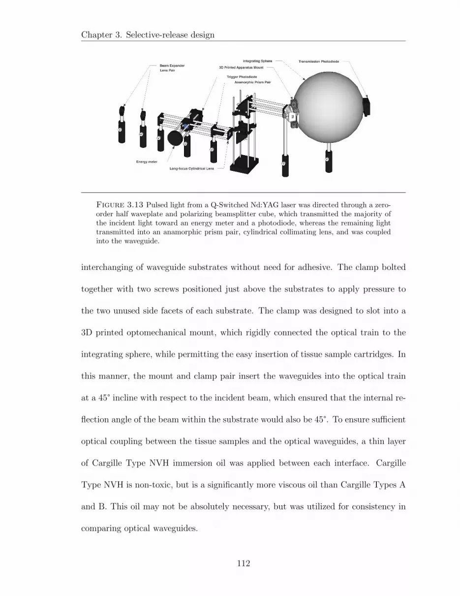
Chapter 3. Selective-release design
Figure 3.13 Pulsed light from a Q-Switched Nd:YAG laser was directed through a zero-order half waveplate and polarizing beamsplitter cube, which transmitted the majority ofthe incident light toward an energy meter and a photodiode, whereas the remaining lighttransmitted into an anamorphic prism pair, cylindrical collimating lens, and was coupledinto the waveguide.
interchanging of waveguide substrates without need for adhesive. The clamp bolted
together with two screws positioned just above the substrates to apply pressure to
the two unused side facets of each substrate. The clamp was designed to slot into a
3D printed optomechanical mount, which rigidly connected the optical train to the
integrating sphere, while permitting the easy insertion of tissue sample cartridges. In
this manner, the mount and clamp pair insert the waveguides into the optical train
at a 45° incline with respect to the incident beam, which ensured that the internal re-
flection angle of the beam within the substrate would also be 45°. To ensure sufficient
optical coupling between the tissue samples and the optical waveguides, a thin layer
of Cargille Type NVH immersion oil was applied between each interface. Cargille
Type NVH is non-toxic, but is a significantly more viscous oil than Cargille Types A
and B. This oil may not be absolutely necessary, but was utilized for consistency in
comparing optical waveguides.
112

Chapter 3. Selective-release design
3.3.4 Experimental methodology
The experimentation was performed by an automated LabVIEW program, which
was designed to control laser operations and data collection, leaving only sample
preparation and signal analysis to the scientist. The software controlled the Q-Switch
delay of the laser, flashlamp activation, and laser firing by means of an RS-232 con-
nection and serial input/output commands. Data was recorded using a 4 channel,
60 MHz bandwidth USB data acquisition device (DAQ; Picoscope, 5442B) operating
with 14 bit resolution. Data acquisition was triggered by the photodiode connected
directly to the optical train, whereas incident laser energy was recorded for each shot
using the USB connected power meter. The LabVIEW software was designed to fire a
single shot and then record the peak photocurrent on channel A, the peak photovolt-
age on channel B, and the incident laser energy from the power meter before repeating
for a total of 200 data points. The laser was fired at approximately 1 Hz to avoid
any potential contamination of data from oversaturated detectors. The photocurrent
was calculated by measuring the voltage drop across a 50 Ω resistor in series with the
photovoltage generated by the photodiode attached to the integrating sphere using a
1X voltage probe.
3.4 Results
The following sections describe the results of optical waveguide transmission
studies performed using ex vivo samples of porcine skin, consisting of epidermal, der-
mal, and adipose tissues. The project progressed in two distinct phases of develop-
ment: (1) empirically establishing the technique as appropriate for light transmission
113

Chapter 3. Selective-release design
Figure 3.14 The SEM-EDS spectrum for silver deposition on silicon substrates at 30 mAfor 240 s resulted in a film over 10 times thicker than that of titanium deposited for thesame duration at higher current, indicating a significantly higher deposition rate for silver.
into tissue, as previous studies had only investigated tissue phantoms, and (2) fabri-
cating a series of waveguides with active area thicknesses increasing at relatively small
increments on the order of a few nanometers to concretely establish the relationship
between film thickness and transmitted intensity.
During the first phase of the project, prior to waveguide fabrication, experiments
were performed to empirically establish the deposition rates of the RF sputter coater
used to clad the fused silica substrates in silver and titanium. These experiments were
performed to obtain an accurate estimation of the film thickness in each active area
without necessitating a direct measurement of every waveguide. SEM-EDS analysis,
a metal film characterization technique discussed in Chapter 2, was performed to
produce elemental spectra for substrates deposited with silver at 30 mA for 60, 120,
180, and 240 s along with those deposited with titanium at 90 mA for the same du-
rations. Figure 3.14 depicts a typical spectrum produced by the SEM-EDS software
for the atomic ratios of a silver film on a silicon substrate deposited for 240 s. The
graph depicts an elemental ratio for Si:Ag of 0.05:1, whereas when deposited for 60 s
114

Chapter 3. Selective-release design
Duration Atomic ratio [Si:Ti] Ti Thickness Atomic Ratio [Si:Ag] Ag Thickness
60 s 60.01:1 7 nm 1.22:1 68 nm
120 s 39.02:1 13 nm 0.35:1 115 nm
180 s 25.00:1 20 nm 0.09:1 190 nm
240 s 19.51:1 25 nm 0.05:1 280 nm
Table 3.1 The tabulated atomic ratios determined by EDS data included alongsidethe corresponding film thicknesses calculated using the NIST DTSA-II spectral analysissoftware.
the ratio if 1.22:1, representing a decrease in interaction between the two elements
with increasing film thickness. Table 3.1 includes the atomic ratios and calculated
deposition rates for each silver and titanium of silicon substrates.
As discussed in Chapter 2, SEM-EDS is not a direct measure of film thick-
ness, but instead relies on comparison of simulated models with experimental data.
Accordingly, film thickness was determined by comparing the EDS spectra recorded
with elemental simulations produced by the NIST DTSA-II software replicating the
experimental conditions. These simulations were iteratively improved and narrowed
until the simulated elemental ratios matched those recorded experimentally. The
corresponding film thicknesses are included in Table 3.1, and were analyzed to deter-
mine deposition rates of 0.104 nm/s for titanium on silicon at 90 mA and 1.17 nm/s
for silver on silicon at 30 mA, assuming linear deposition rates due to RF sputtering
occurring with constant current.
After establishing metal film deposition rates, waveguides were fabricated with
active area film thicknesses of 0, 10, 20, and 30 nm, with 0 nm representing the bare
substrate acting as the experimental control. Light was transmitted through the tissue
samples and was recorded as a peak photovoltage intensity by the integrating sphere
photodiode and the trigger photodiode. Owing to difficulties with the LabVIEW
115

Chapter 3. Selective-release design
−5 0 5 10 15 20 25 30 350.5
0.6
0.7
0.8
0.9
1
1.1
1.2
1.3
Active area film thickness [ nm ]
Cor
rect
ed tr
ansm
itted
inte
nsity
[ V
/V ]
Corrected transdermal laser intensity regulated by film thickness
Student Version of MATLAB
Figure 3.15 Preliminary experiments confirmed that the transmission of light throughex vivo samples of porcine skin decreased with increasing optical film thickness, as waspredicted.
software provided by Thorlabs for the USB energy meter, pulse-to-pulse variations
in laser intensity were corrected for by dividing the peak photovoltage of the sample
photodiode by that of the trigger photodiode. Figure 3.15 depicts the results of this
study, and demonstrates a distinct decrease in optical transmission with increasing
film thickness, as was expected based on our prior work with optical tissue phantoms.
The data from phase 2 of this project is currently being collected and ana-
lyzed and will be incorporated into a later draft of this dissertation. A plot of the
transmission of the ten waveguides is included in Figure 3.16; however, we are cur-
rently attempting to collect cleaner data with narrower error bars. It should be noted
that this data was analyzed prior to our current laser energy measurement correction
116

Chapter 3. Selective-release design
−10 0 10 20 30 40 50 60 700.8
1
1.2
1.4
1.6
1.8
2
2.2
2.4
2.6
Active area thickness [nm]
Ener
gy
corr
ecte
dphoto
curr
ent
[mA
/m
A]
Mean transmission vs. Active area thickness
1
Figure 3.16 The transmission of light through thin film active areas decreases with in-creasing film thickness; however, the current data suggests that ultra thin films demonstratea local minimum, which increases around 20 nm and then drops off rapidly thereafter.
paradigm, as discussed in Appendix C, so we will also be re-evaluating the data based
on the new method of analysis.
3.5 Discussion
The principal ramification of the preliminary results included in Figure 3.15,
is that they immediately demonstrated the potential for the waveguide technology
to be utilized in tissue-based applications; whereas previous studies had been lim-
ited to artificial tissue simulations. The isolated and enclosed nature of the optical
apparatus and photodiode within the integrating sphere concretely established that
the waveguides each successfully transmitted light through the 4 mm thick samples of
117

Chapter 3. Selective-release design
tissue Moreover, the decreasing transmission with respect to increasing film thickness
suggests that the light underwent frustrated total internal reflection within the active
area, which was regulated by controlling active area film geometry. An additional
implication of the success of the preliminary data regarded the elimination of the
operating distance between the laser source and the tissue. These results indicated
contact-based transmission to be a viable technology, at least for the comparatively
low intensities utilized in this study.
More recent optical transmission studies have been performed using waveguides
with active area geometries from 0 – 60 nm in increments of 5 nm and have demon-
strated some success; however, we have had problems with the reliability of the optical
alignment and are currently revising our approach and collecting new data, which will
be analyzed and incorporated into this dissertation. We have also recently serviced
the laser by replacing the flashlamp and deionization cartridge, which will ideally
improve the performance and reliability of the laser.
118

Chapter 4
Simultaneous paraxial ultrasonic pulsationto improve transdermal laser fluence
Portions of this chapter have been reproduced with permission from the manuscript
entitled Ultrasonic Modulation of Tissue Optical Properties in Ex Vivo Porcine Skin
to Improve Transmitted Transdermal Laser Intensity, authored by Paul J.D. White-
side, Chenxi Qian, Nicholas J. Golda, and Heather K. Hunt, published in the journal
Lasers in Surgery and Medicine [155].
4.1 Introduction
Over the past few decades, the increasing demand for minimally invasive tech-
niques for clinical or surgical applications has led to the development of a wide array
of transdermal laser-based technologies. These technologies have been used for tissue
resurfacing, tattoo and hair removal, treatment of pigmentary disorders, photother-
mal tumor ablation, and the treatment of vascular lesions [2–4, 156]. The broad
variety of optical therapeutic procedures is credited primarily to the laser devices’
narrow wavelength bandwidth, which permits the specific targeting of individual
chromophores based on their relative optical absorption spectra [2, 5]. For exam-
119

Chapter 4. Sonoillumination
ple, the removal of green tattoo inks is typically best performed using either red or
near-infrared laser light, owing to the tendency of green inks to absorb strongly in
those wavelength regimes as compared to their absorption at shorter wavelengths in
the ultraviolet to yellow regimes [8, 16].
However, for any given application, it is unlikely that the laser light will be
perfectly, selectively absorbed by only the target of choice. Although the wavelength
may be specifically chosen for greatest impact on the therapeutic target, there will
inevitably be additional chromophores interspersed throughout the dermis and epi-
dermis that may also absorb at the chosen wavelength. The three most predominant
biological chromophores that detrimentally impact the efficacy of optically based pro-
cedures are hemoglobin, melanin, and water; a number of additional proteins and
enzymes have been shown to absorb light within the UV spectrum as well [157–159].
Hemoglobin, melanin, and water vary in concentration based on both the patient’s
skin type and the relevant anatomical region; however, their absorptive properties,
and therefore their impact on the procedure, are dependent upon only their molec-
ular structure. Accordingly, each of these molecules exhibits a different absorption
spectrum, as shown in Figure 4.1, with melanin absorbing strongly throughout the
visible spectrum and hemoglobin demonstrating two slightly different spectra based
on its state of oxygenation [160, 161]. In the event that one or more of these spectra
overlaps with that of the clinical target at the chosen wavelength, their presence in
the tissue above the target will necessarily detract from the efficacy of the procedure
not only by reducing the amount of light that reaches the target, but also by generat-
ing undesirable photothermal effects, such as carbonization and inflammation, which
120

Chapter 4. Sonoillumination
Figure 4.1 Whereas melanosomes in human skin are on average broadly absorbingthroughout a wide range of wavelengths, hemoglobin exhibits peaks and valleys in bothoxygenated and deoxygenated spectra, which may be exploited when selecting lasing wave-length.
thereby further exacerbate the attenuation of light [9, 35, 43].
The clinical solution to this problem is typically to either increase the incident
laser energy or otherwise reduce the laser spot size, both of which increase the laser
energy density that reaches the clinical target [22]. Such practices serve as an ex-
pedient solution for an immediate clinical problem; however, they also intensify the
detrimental side effects presented by unintended optical targets. This is particularly
concerning in the case of epidermal melanin absorption. Melanin is a broadband op-
tical absorber produced within the surface epidermal tissue, and is therefore likely
to reside in the path between the laser source and the clinical optical target. Un-
surprisingly, the efficacy of light-based techniques decreases dramatically for patients
121

Chapter 4. Sonoillumination
with higher concentrations of melanin (i.e. skin types higher on the Fitzpatrick scale)
[162]. Moreover, the side effects resultant from melanin absorption also increase with
local energy density, which can result in scarring or localized pigmentary changes
(hypo- or hyperpigmentation) [56]. The combination of these two concerns renders
most optical therapeutic techniques increasingly ineffective for a substantial portion
of the global population.
Previous research has attempted to address this problem by optically clearing
the tissue via chemical or mechanical means. For instance, a number of chemical opti-
cal clearing agents (OCA) have been investigated to increase optical transmittance in
laboratory imaging techniques like Optical Coherence Tomography (OCT), including
glycerol, glucose, polypropylene glycol (PPG), polyethylene glycol (PEG), dimethyl
sulfoxide (DMSO), and oleic acid . However, for potential clinical applications, glyc-
erol is typically preferred as it is biocompatible and considered a safe chemical agent
by the Food and Drug Administration [163, 164, 164, 165]. Yoon et al. demonstrated
that the tissue optical clearing (TOC) effects of glycerol may be further improved
by physically overcoming the barrier presented by the stratum corneum using a mi-
croneedle roller to introduce artificial microchannels in the tissue followed by the
application of sonophoresis, which ultrasonically induces microcavitation within the
tissue along with thermal and mechanical effects that help to promote permeability
of OCAs into the tissue [166–169].
Purely mechanical methods have also been demonstrated; these aim to avoid
any long-term chemical clearing by mechanically altering the tissue’s local optical
properties. Rylander et al. demonstrated two such mechanically-based tissue optical
122

Chapter 4. Sonoillumination
clearing devices (TOCD), one of which used an array of mechanical pin transducers
to induce localized vacuum pressure, whereas the other used an array of ball lenses to
focus light into the tissue while applying a vacuum pressure in the interstices between
lenses [170]. Both of these TOCDs utilized the vacuum to stretch and compress
the tissue while under radiant exposure, thereby displacing interstitial water and
blood within the tissue and increasing light fluence through porcine skin samples
[171]. Their work suggested that mechanical modification of optical properties had
the potential to improve radiant throughput by reducing optical path length and
potentially displacing chromophores.
Although both paradigms to tissue optical clearing have proven effective in prior
investigations on in vitro, ex vivo, and in vivo tissues, each method presents poten-
tially limiting factors or detrimental side effects. Of the two approaches, OCAs have
been much more broadly investigated, which has yielded reports that their efficacy
varies strongly with concentration. Even agents such as glycerol, which are considered
relatively “safe,” have been shown to significantly alter tissue structure or obstruct
localized blood flow in high concentrations, while insufficiently clearing the tissue at
lower concentrations; other OCAs may induce edema or suppuration, or result in tis-
sue scarring [165]. Moreover, even when appropriate concentrations are utilized, the
barrier presented by the stratum corneum often prevents or prolongs topical diffusion
of OCAs into the tissue, which may necessitate invasive hypodermal injection of the
OCA or lengthy pre-treatment with sonophoresis in order to effect optical clearing
[172]. By contrast, mechanical TOCDs represent a relatively recent technology and
accordingly have seen very limited development. Although publications have been
123

Chapter 4. Sonoillumination
generally positive, their efficacy in clinical therapeutics has yet to be demonstrated
and improvements in transmitted intensity are postulated as related to observed de-
creases in optical scattering, tissue thickness, and changes in group refractive index
[171].
Therefore, the purpose of this research was to develop an alternative tissue opti-
cal clearing technique that would be predominantly mechanical in nature, but which
could also be utilized alongside the application of an OCA if necessary. Whereas the
aforementioned research by Yoon et al. involved the use of ultrasound to improve the
diffusion of OCAs into the skin, the work presented herein instead focused only on
the mechanical action of ultrasonic pulsation to locally alter the optical properties
of the tissue through periodic compressions and rarefactions [173]. This technique
builds upon precedent established by low intensity Ultrasound-Modulated Optical
Tomography (UOT), wherein continuously pulsed ultrasound results in changes in
mass density and the corresponding optical properties (i.e. refractive index, scat-
tering coefficient, absorption coefficient), and changes in optical phase due to the
displacement of scatterers and absorbers [174].
4.1.1 Objectives
Unlike sonophoresis-based methods, which are applied prior to laser treatment,
this work investigated the potential for continuously pulsed ultrasound to mechan-
ically modify the tissue throughout the course of the procedure. However, in es-
tablished UOT publications, the ultrasound is typically applied to ex vivo tissue
samples in water baths perpendicular to the direction of optical transmission, which
124

Chapter 4. Sonoillumination
Figure 4.2 Using an optical waveguide permits the paraxial application of ultrasonicpulsation, which modulates the tissue’s optical properties to improve transdermal lasertransmission.
is patently not an option for any clinical application. To resolve this issue, planar
optical waveguides were used to transmit laser light directly into the tissue through
physical contact, which permitted the paraxial application of ultrasonic pulsation on
the rear face of the waveguide, as shown in Figure 4.2 [175]. Although both these
techniques had previously been independently established, this project hypothesized
that their paraxial application might sufficiently alter the optical properties of the
tissue such that total intensity of transmitted light through epidermal, dermal, and
adipose tissue would be substantially increased.
As such, Q-switched Nd:YAG laser, similar to those used in clinical dermatol-
ogy, was used to transmit pulses of light at a wavelength of 532 nm into samples of
ex vivo porcine skin by means of a silvered acrylic optical waveguide, based on de-
125

Chapter 4. Sonoillumination
signs established in prior investigations [1, 66, 83]. The light was confined within the
waveguide until reaching a pre-defined active area in contact with the tissue, where-
after the light refracted into the skin. Ultrasound was then applied on the rear face
of the waveguide at a frequency of 510 kHz, varying the amplitude to determine what
effect, if any, the ultrasound might have upon the transmission of light through the
tissue.
4.2 Phenomenological model
Figure 4.2 depicts a theoretical means of implementing sonoillumination in
which acoustic pressure is applied to the tissue by means of an ultrasonic trans-
ducer. The acoustic waves are coupled into the tissue through an optical selective
release waveguide (SRW), which concept was discussed in Chapter 3. Moreover, the
SRW simultaneously irradiates the tissue with light, which propagates through the
ultrasonically modulated medium. The following phenomenological model represents
the current understanding of the methods by which sonoillumination improves opti-
cal transmission through epidermal, dermal, and adipose tissues; although, the same
principles can be translated to applications for other tissues and non-biological media.
4.2.1 Established acousto-optic theory
The ultrasonic modulation of transparent and turbid media for optical benefit
has been extensively demonstrated in the realms of acousto-optics and ultrasound-
modulated optical tomography. Accordingly, the discussion of the mechanisms of
sonoillumination are founded on established acousto-optic theory coupled with em-
126

Chapter 4. Sonoillumination
pirical observations recorded in lab.
Acousto-optics (A-O), not to be confused with opto-acoustics, principally re-
gards the modulation of optical properties of transparent media by means of ultra-
sonic pulsation, and has been implemented to generate acoustically-induced diffrac-
tion gratings, deflectors, and optical modulators [141, 176, 177]. In such applications,
acoustic pressure induces regional changes in optical refractive index within the re-
gions of applied acoustic pressure, which will form a column when applied using an
unfocused transducer or a hyperboloid when using a focused transducer, with the
waist of the hyperboloid located at the focal point of the transducer. This change in
refractive index is resultant from an acoustically induced strain within the medium,
which alters the medium’s local permittivity by means of varying the local material
density [178]. Considering the strong relationship between material density and opti-
cal refractive index, which is a measure of the relative speed of light within a medium,
any density alterations within a medium necessarily change the local relative speed
of light due to an increase or decrease in the amount of material per unit of space
that is present to hinder light transmission, leading to a direct relationship wherein
∆n/n = ∆ρ/ρ [179].
When the acoustic field applied to a medium is nearly orthogonal to the inci-
dent light, the acoustic waveform can induce a gradient refractive index field (GRIF)
consisting of intermittent regions of high pressure followed by comparatively low pres-
sure, which forms a diffraction grating moving with the velocity of the acoustic wave
in the medium [180]. For a plane wave propagating along the z-axis in a transparent
medium, the refractive index becomes a function of both depth, z, and time, t, and
127

Chapter 4. Sonoillumination
can be expressed as Eq. 4.1,
n(z, t) = n0 −∆n cos (Ωat− kaz) (4.1)
wherein: ∆n =1
2pzjn0
3S0 (4.2)
in which Ωa is the angular frequency (2πf) and ka is the acoustic wavenumber (2π/λa),
∆n is the amplitude variation in the refractive index, S0 is the amplitude of the
acoustically-induced mechanical strain, and pzj is the photoelastic constant (i.e. the
strain-optic coefficient) [178]. These equations are simplified and assume that the
acoustic pressure is applied orthogonal to the surface of the medium by an unfocused
acoustic source, and that the medium is homogenous. As such the equations omit
deviations in the x- and y- directions; however, in practice, such deviations will oc-
cur due to inhomogeneities in the media involved. Additionally, the negative value
indicates that a positive strain corresponds with a decrease in refractive index.
According to Eq. 4.1, the acoustic wavenumber, ka, is a determining factor
with regard to the depth-resolved change in refractive index. The ramification of
this relationship is that the diffractive or deflective effects are directly affected by the
properties of the acoustic waveform, including its amplitude, frequency, and wave-
length, since ka = 2πf/cs, wherein f represents the acoustic pulsation frequency and
cs represents the speed of sound in the medium. This distinction has led to frequency
regimes of differing effects, with Raman-Nath diffraction and Bragg diffraction. The
128
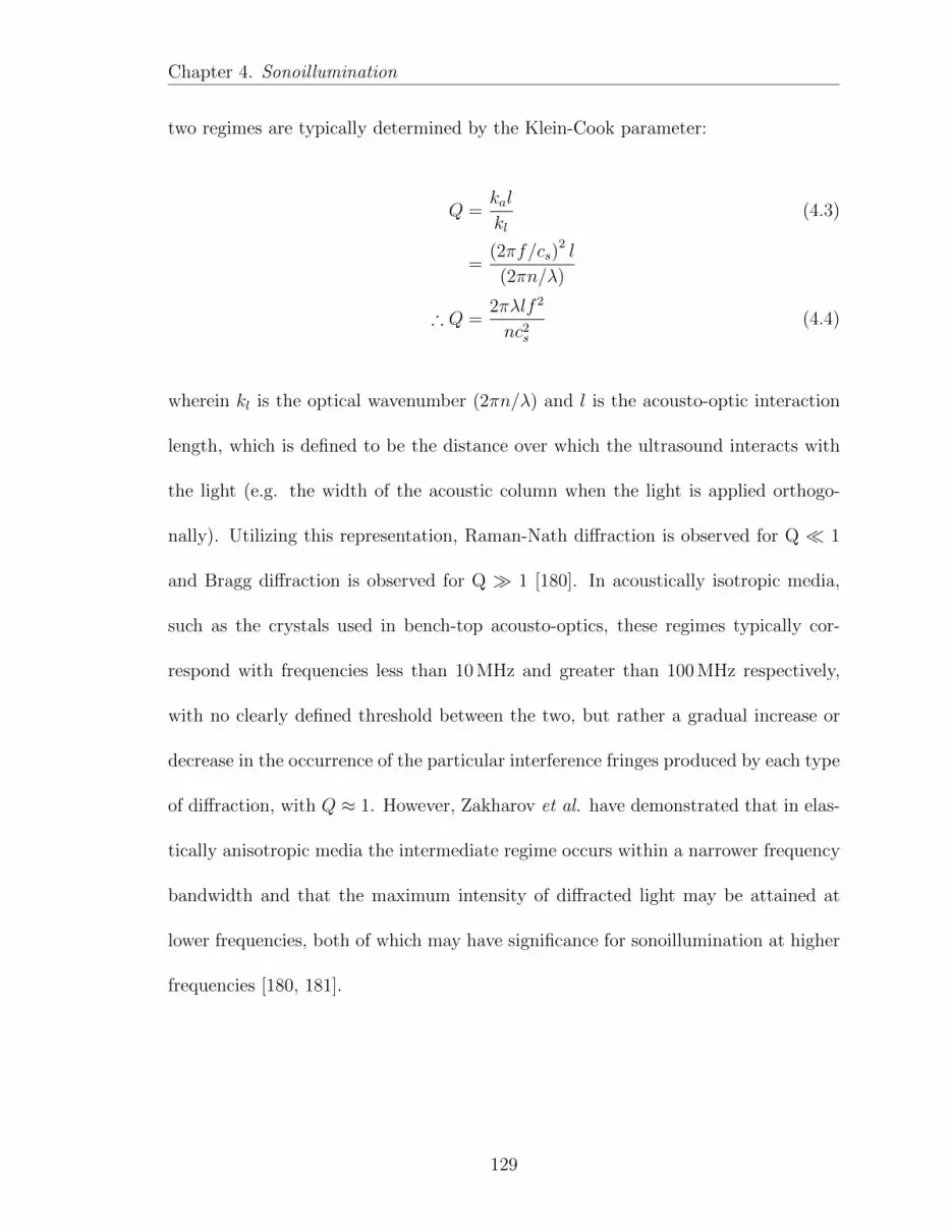
Chapter 4. Sonoillumination
two regimes are typically determined by the Klein-Cook parameter:
Q =kal
kl(4.3)
=(2πf/cs)
2 l
(2πn/λ)
∴ Q =2πλlf 2
nc2s
(4.4)
wherein kl is the optical wavenumber (2πn/λ) and l is the acousto-optic interaction
length, which is defined to be the distance over which the ultrasound interacts with
the light (e.g. the width of the acoustic column when the light is applied orthogo-
nally). Utilizing this representation, Raman-Nath diffraction is observed for Q 1
and Bragg diffraction is observed for Q 1 [180]. In acoustically isotropic media,
such as the crystals used in bench-top acousto-optics, these regimes typically cor-
respond with frequencies less than 10 MHz and greater than 100 MHz respectively,
with no clearly defined threshold between the two, but rather a gradual increase or
decrease in the occurrence of the particular interference fringes produced by each type
of diffraction, with Q ≈ 1. However, Zakharov et al. have demonstrated that in elas-
tically anisotropic media the intermediate regime occurs within a narrower frequency
bandwidth and that the maximum intensity of diffracted light may be attained at
lower frequencies, both of which may have significance for sonoillumination at higher
frequencies [180, 181].
129

Chapter 4. Sonoillumination
4.2.2 Established UOT theory
Bench-top A-O typically involves the use of optically transparent media to
induce an acoustically variable diffraction grating; however, ultrasound-modulated
optical tomography (UOT) employs the techniques to improve imaging in ex vivo
tomography of tissue structures [179, 182, 183]. Optical tomography traditionally
suffers resolution losses due to scattering-induced destructive optical interference at
the detector, which effect is referred to as “speckle” [184]. Although A-O focuses on
modulating refractive index, in UOT ultrasonic pulsation is applied to ex vivo tissue
samples to modulate the position of scattering elements within the tissue and thereby
alter the speckle effects observed at the detector interface [185].
In addition to refractive index changes, the applied acoustic pressure wave also
displaces optically scattering and absorbing matter within the medium [185]. Al-
though the displacement is typically very small, on the order of tens or hundreds
of nanometers, it is sufficient to periodically alter the conditions of optical collision
events, which results in the blurring of the observed speckle. Moreover, the modula-
tion of scatterer position can also result in a phase modulation of the optical field and a
Doppler-shift in the optical frequency corresponding to the magnitude and frequency
of the scattering wavevector [186]. This Doppler-shift can result in the generation of
“acoustic sidebands” that are located as multiples of the acoustic propagation fre-
quency around the primary incident laser frequency. In UOT, the Doppler-shift can
be significant for reducing speckle in image formation, because frequency-shifted pho-
tons are less capable of destructively interfering with the primary optical frequency,
130

Chapter 4. Sonoillumination
Figure 4.3 In sonoillumination, pulsed ultrasound is applied by an (a) an ultrasoundsource, via (b) an optional acoustic couplant, into (c) an optical selective-release waveguide,which transmits both light and acoustic pressure into (d) the target medium.
which can blur and effectively fill-in the imaging gaps left by destructive speckling.
4.2.3 Mechanisms of sonoillumination
The mechanisms of sonoillumination build on the principles established by
acousto-optics and ultrasound-modulated optical tomography, while also represent-
ing a significant deviation from both. Figure 4.3 represents a theoretical diagram
of sonoillumination theory, which incorporates both (1) regional changes in optical
refractive index as predicted by acousto-optics, and (2) the displacement of optically
scattering and absorbing matter as employed in UOT; however, sonoillumination
also incorporates two additional effects regarding the anisotropy of the tissue and
131

Chapter 4. Sonoillumination
a frequency-dependent relationship with the transport mean free path of the light
through the turbid medium, which will be discussed below.
4.2.3.1 Refractive index modulation
With regard to differentiating sonoillumination from the two established techniques,
applications of A-O and UOT typically utilize cases wherein the angle between the
incident light wavevector and the acoustic wavevector, represented in Figure 4.3 as
θA, is relatively close to orthogonal (i.e. close to π/2) [141]. In A-O, this permits the
light to transmit through the acoustically-induced pressure zones as if it were trans-
mitting through a physical diffraction grating, with the distinct advantage of being
able to change the properties of that grating in real time by altering the pulsation fre-
quency, magnitude, or timing with respect to laser operation. Moreover, in UOT, the
orthogonally applied acoustic pressure effectively shortens the magnitude of the scat-
tering wavevector and thereby reduces the impact of collision events and destructive
interference on the detected image. However, for the purposes of sonoillumination,
the effective angle of incidence between the light transmitted into the medium and
the acoustic propagation vector is of substantial significance. Specifically, in the the-
oretical diagram shown in Figure 4.3, the angle between the acoustic propagation
vector and the incident light vector is significantly less than π/2, which permits the
acoustically varying GRIF generated within the tissue to behave less like a diffraction
grating and more like a gradient refractive index lens (GRIN), continuously refracting
the light as it propagates through the tissue.
Akin to the effect explained by Eq. 4.1 in transparent media, the GRIF is de-
132

Chapter 4. Sonoillumination
pendent upon the amplitude variation in the refractive index and the induced strain,
both of which are directly dependent upon the applied acoustic waveform. For ex-
ample, a continuous sinusoidal waveform, such as is depicted in Figure 4.3, induces
a field that continuously changes from regions of greater density to those of lower
density, with GRIF characteristics corresponding to those of the applied acoustic
pressure with regard to frequency, wavelength, waveform, amplitude, and the direc-
tion of the acoustic propagation vector. Accordingly, the varying refractive index field
may cause the incident light to undergo subsequent refraction throughout the tissue
in a manner similar to light transmission through a physical GRIN lens, wherein the
light propagation vector bends as it transmits through the continuous gradient [187].
Since the GRIF is not a physical constant, but is instead induced by means
of a temporally and spatially variant acoustic waveform, differing applications may
benefit from applying the GRIF such that it exhibits a desired refractive index or
relative pressure at a specific location within the medium. For example, the GRIF
may be applied such that there is a local refractive index maximum at the surface of
the tissue, which would alter the optical boundary conditions between the tissue and
external medium, thereby decreasing the optical reflection coefficient and the angle
of refraction. Alternatively, the GRIF may be applied to exhibit a maximum at a
defined distance below the surface in order to apply a mechanical strain to a specific
optical target to improve a desired therapeutic effect, such as the photomechanical
ablation of tattoo ink located within the dermis.
133

Chapter 4. Sonoillumination
4.2.3.2 Alteration of optical collision events
In addition to refractive index effects, the applied ultrasound also modulates the
position of scatterers within the tissue, which can have a variety of ramifications
that collectively contribute to improving optical transmission. As in UOT, the dis-
placement of scatterers can result in a Doppler-shift in the frequency of the applied
photons. Although the Doppler-shift is at least seven or eight orders of magnitude
smaller than the primary optical frequency, which will have negligible impact with
regard to the absorption spectrum of the clinical target, the corresponding reduction
in possible destructive interference may permit a greater portion of the incident light
available to transmit toward the target. For applications employing multiple succes-
sive laser pulses incident upon the same location, the temporally variable acoustic
field displaces scatterers differently for successive laser pulses, which may also allow
light to transmit to portions of the target missed by previous shots.
Another effect that is observed regards the shortening of the scattering wavevec-
tor in low pressure acoustic zones [185]. The same displacement that results in a
decrease in the energy of the colliding photon and corresponds to the lower acoustic
sidebands also reduces the magnitude of the optical wavevector following scattering
events within low pressure zones. By contrast, in high pressure zones, the applied
pressure incorporates the magnitude and directionality of the acoustic wavevector into
the deflected optical wavevector [188]. This results in the generation of the higher
acoustic sidebands, but also deflects the optical wavevector in the direction of the
acoustic wavevector by transferring the mechanical energy of the displacement into
134

Chapter 4. Sonoillumination
the colliding photon. Extrapolating that assertion suggests that the applied pressure
field skews the anisotropy of the tissue in the direction of the acoustic wavevector.
The anisotropy of a turbid medium is defined to be the average cosine of the deflection
angle following a scattering event, g =< cos(θ) >, which is therefore a value between
−1.0 and 1.0, wherein a magnitude of 0 represents a perfectly isotropic medium and a
magnitude of 1.0 represents a perfectly forward or backscattering medium [189]. With
regard to biological tissue, anisotropy is typically between 0.8 − 1.0, representing a
largely forward-scattering medium, and is often considered to be around g = 0.90
[189, 190]. Consequently, if sonoillumination increased the forward anisotropy, there
would be a corresponding increase in the likelihood that the clinical target would
receive a greater dose of the applied light.
Each of the aforementioned effects are fundamentally tied to the properties of the
applied pressure field, and are therefore strongly related to the magnitude, frequency,
and propagation vector of the acoustic waveform. The impact of each property,
however, is theorized to reach individual thresholds beyond which their influence
either plateaus or begins to operate under distinctly different conditions. For example,
with regard to acoustic magnitude, this threshold represents the maximum degree to
which the tissue may be manipulated before necessitating a physiological change to the
medium. In other words, the ultrasound does not remove the scatterers or absorbers,
nor does it introduce any additional material into the medium or change its phase;
accordingly, it can only modulate its properties so much before the modulation ceases
to result in a measurable change in optical properties. Increasing the magnitude
beyond this threshold likely results in minimal change in optical properties until such
135

Chapter 4. Sonoillumination
point as the overall structure of the medium is fundamentally altered, as occurs in
sonophoresis through the ultrasonically-induced generation of hollow microcavities
from dissolved gas [169].
Moreover, with regard to the propagation vectors, the theoretical threshold
represents the distinction between the GRIF behaving less like a GRIN lens and
more like a diffraction grating or GRIN optical fiber. Unlike traditional optical fibers
that rely on internal reflection between core and cladding materials, GRIN optical
fibers refract the light continuously within the cylindrical gradient index substrate,
bending the light vector between the higher refractive index center and the lower
refractive index exterior regions [191]. In tissue, the parallel regions of high and low
refractive index could behave in a manner akin to GRIN fibers for sufficiently large
values of θA at low frequency and thereby “guide” the light deeper into the tissue as
if it were transmitting through a biological waveguide. This effect is anticipated to
occur at lower frequencies <1 MHz, as it will likely behave more like traditional UOT
or A-O at higher frequencies. The theorized propagation vector threshold represents
the angle between the optical and acoustic wavevectors, such that there is a transition
between the GRIN lens region and the GRIN fiber region. Since the relative angle
between the wavevectors is of greater importance than their direction with respect to
the tissue, orthogonal incidence may be achieved by applying both light and acoustics
at an angle to the skin or by refracting the acoustic wave into the tissue using an
acoustic wedge. Literature review has not yielded evidence of any such behavior,
which is tentatively attributed in part to the relative youth of ultrasonic modulation
but is also suspected to be related to the high frequency nature of contemporary
136

Chapter 4. Sonoillumination
approaches, which seek to achieve diffractive effects or to modulate speckle, rather
than to guide transmission.
Finally, based on the inverted relationship between acoustic pulsation frequency
and the distance between successive pressure wavefronts (i.e. the acoustic wave-
length), there will likely be a strong positive correlation between acoustic frequency
and the likelihood that the sonoillumination effects will influence the propagation of
any given photon. This relationship is based on the comparison of the acoustic wave-
length for typical ultrasound in tissue, which for frequencies from 15 kHz to 100 MHz
is between 10.63 cm and 15.95 µm respectively (assuming cs =1595 m/s), with the op-
tical transport mean free path length (TMFP) of the incident light within the tissue,
which is typically around 1 mm for visible light [174, 192]. The TMFP, also referred
to as the “reduced mean free path,” represents the average distance a photon will
travel in tissue before losing “direction memory,” after which it can be considered
a randomly propagating photon, rather than part of an incident beam [190]. The
TMFP can be calculated from the standard optical mean-free path length, which is
the average distance a photon will travel between scattering events, as follows:
lmfp =1
µs(4.5)
µ′s =µs ∗ (1− g) (4.6)
l′mfp =1
µ′s ∗ (1− g)(4.7)
∴ TMFP =lmfp
(1− g)(4.8)
137

Chapter 4. Sonoillumination
wherein µs represents the scattering coefficient, lmfp is the mean free path length,
g is the anisotropy of the tissue, and µ′s is the reduced scattering coefficient l. As
mentioned above, the photon loses direction memory after one TMFP into the tissue,
which consequently often represents the limit for optical imaging techniques in tissue.
However, since the typical TMFP for visible light is within the realm of available
acoustic pulsation wavelengths, when the two are of comparable length, there is a
much higher likelihood that the acoustic pulsation will influence the propagation of
the photon. Assuming a TMFP of 1000 µm, the corresponding ultrasonic pulsation
frequency is approximately 1.595 MHz. Based on these assertions, for frequencies
less than 1.595 MHz, the impact of sonoillumination on photon migration will be
largely due to modulation of refractive indices near the surface of the tissue; however,
beyond this threshold frequency, each photon is increasingly likely to be impacted
by the sonoillumination’s effect on at least one collision event. Moreover, based on
the same TMFP and the previously mentioned anisotropy of tissue, the typical MFP
is on the order of 100 µm. As such, there may be a second threshold frequency
at 15.95 MHz, since the distance between wavelengths would be comparable to the
distance between individual scattering events, which represents a significant likelihood
that the conditions of every collision event will have been altered by sonoillumination.
Correspondingly, Table 4.1 includes the typical TMFP for a variety of biological
tissues along with the corresponding acoustic frequency at the primary and secondary
thresholds to anticipate the divisions of regimes based on tissue [174, 190].
138

Chapter 4. Sonoillumination
Tissue TMFP Primary threshold Secondary threshold
Muscle 1.1 mm 1.45 MHz 14.5 MHz
Skin 1.0 mm 1.595 MHz 15.95 MHz
Brain 0.6 mm 2.658 MHz 26.58 MHz
Breast 0.8 mm 1.994 MHz 19.94 MHz
Lung 0.3 mm 5.317 MHz 53.17 MHz
Table 4.1 Typical TMFP in various tissues listed with corresponding acoustic frequen-cies at the primary threshold, wherein the wavelength corresponds to the TMFP, and thesecondary threshold, wherein the wavelength corresponds to the MFP [174, 190].
4.3 Materials and methods
Although the amplitude, frequency, and propagation angle are each likely to
have significant influence on the method and efficacy of sonoillumination, due to
the limitations of the equipment available, the experiments performed herein exclu-
sively investigated the effect of varying the magnitude of acoustic pulsation on optical
transmission. The following sections describe the procedures involved in waveguide
fabrication and tissue sample preparation, along with a description of the optical ap-
paratus employed in the associated experiments. Additionally, details regarding the
ultrasonic pulsation electronics are also included.
4.3.1 Porcine tissue samples
Large sections of ex vivo porcine skin were donated for this research project from
the Mizzou Meat Market (College of Agriculture, Food, and Natural Resources at the
University of Missouri). The skin was disinfected in a 1.75% ethanol solution for 2
minutes prior to processing for experimentation. Following disinfection, the sections
were trimmed down to a thickness of 4 mm, incorporating epidermal, dermal, and
139

Chapter 4. Sonoillumination
Figure 4.4 3D printed cartridges were designed to keep the porcine skin taut duringexperimentation while also allowing for consistent and easy interchanging of samples.
adipose tissue, and cut into 40 mm square samples. Originally, each sample was
held taut and adhered at the edges with superglue over a thin fiberglass mesh to
individual 3D-printed tissue mounts, as shown in Figure 4.4, which incorporated
open apertures to allow for measurement of optical transmission through the tissue.
The fiberglass mesh was included to provide additional support to the porcine skin
and prevent potential indentation of the tissue during testing. Processed skin samples
were wrapped in moist Kim wipes to prevent dehydration, enclosed in air-tight plastic
bags, and stored in a freezer at 4°C until needed. Prior to use, samples were defrosted
by running water over the plastic bag for 10 – 15 min.
4.3.2 Waveguide fabrication
The optical waveguides were fabricated in-house from a large sheet of 1.5 mm
thick polymethyl-methacrylate (PMMA) acrylic glass (Evonik CRYO, 0A000 GT).
Waveguide substrates were cut into 28 x 25.5 mm units and machined to incorporate
45 angled faces at two opposing ends, as shown in Figure 4.5. Both of the angled
140

Chapter 4. Sonoillumination
Figure 4.5 A planar optical waveguide composed of a PMMA substrate clad in thin filmsof silver ensured internal reflection angles of 45° and enabled the transmission of laser lightinto porcine tissue through direct physical contact with the exposed “active area” on thewaveguide’s largest face.
faces and the two largest faces were polished using optical sanding paper with 200,
800, 1000, and 2000 grits in increasing order, followed by a final polish using a fine
scratch removing compound (Novus Fine Scratch Remover No. 2). The two angled
entrance and exit apertures of the substrates were masked off with Kapton tape, along
with a 9 mm x 25.5 mm rectangular section of the largest face, which would serve as
the waveguide’s active area. The substrates were then clad in thin films of titanium
and silver using a cold sputtering vacuum deposition system (Quorum Technologies,
K575X) to serve as mirrors on the bounding surfaces of the substrate. The titanium
was deposited using a 99.998% pure Ti target at 90 mA for 60 s, which formed a film
less than 10 nm thick. The titanium acted as an adhesion layer for the silver, which
141

Chapter 4. Sonoillumination
Figure 4.6 Laser light at 532 nm triggered data collection, was measured for pulse-to-pulse energy variations, and was then transmitted through porcine skin into an integratingsphere by a planar waveguide. Ultrasound was applied to the rear face of the waveguide,driven by an AWG, amplified 50 dB, and impedance matched to improve electrical trans-mission. Light was detected by a reverse-biased photodiode, whose photovoltage spike wasmeasured by a voltage probe across a series resistor, R.
was deposited from a 99.95% pure Ag target at 30 mA for 300 s to form a much thicker
layer approximately 200 nm thick. Laser light incident perpendicularly upon one of
the angled faces would internally reflect along the waveguide to the exit aperture
when exposed to air, but would transmit out through the active area when in contact
with tissue.
4.3.3 Experimental apparatus
The goal of these experiments was to investigate the potential for increased
light fluence through epidermal, dermal, and adipose tissues under continuous ultra-
sonic pulsation with relevance to potential clinical applications in laser dermatology.
Accordingly, pulsed laser light, generated by a Q-switched Nd:YAG laser (Opotek,
142

Chapter 4. Sonoillumination
Vibrant 355 II) operated at a wavelength of 532 nm with a 5 ns pulse width, was
transmitted through porcine skin samples and measured using a reverse-biased Si
photodiode (Thorlabs, DET100A) attached to an integrating sphere. The light was
guided into the tissue using silvered optical waveguides following a short optical train
that modified the beam shape to better suit a planar waveguide and directed light
toward a second photodiode to trigger data collection and a power meter to account
for variations in pulse-to-pulse laser intensity. The optical train, shown in Figure
4.6, consisted of a zero-order half-waveplate (Thorlabs, WPH05M-532) and polar-
izing beamsplitter cube (Thorlabs, CM1-PBS251) to direct a small portion of light
toward the trigger photodiode (Thorlabs, DET10A), while transmitting the remain-
ing s-polarized light along the length of the train. A standard 50:50 beamsplitter
cube was used to direct half of the beam intensity toward a power meter (Thorlabs,
PM100USB) and the remaining half toward a 4X anamorphic prism pair (Thorlabs,
PS883-A), which compressed the beam along one axis to transform the incident cir-
cular beam into an elliptical Gaussian profile approximately 1.5 mm thick along its
narrow axis. To compensate for the dispersive effects caused by the extreme degree
of compression, a long focus cylindrical lens (Thorlabs, LJ1558L2-A) re-collimated
the beam prior to entering the waveguide.
The waveguides were fixed at a 45° incline with respect to the incident beam
using a custom 3D printed optomechanical mount (Figure 4.7) that rigidly connected
the optical train to the integrating sphere while allowing for interchangeable tissue
samples and waveguide cartridges. At this incline, the incident light was perpendicu-
lar to the angled face of the substrate, which minimized refraction and ensured that
143

Chapter 4. Sonoillumination
Figure 4.7 The waveguides were sealed into 3D printed mounts to ensure consistentalignment between tests while permitting the ultrasound transducer to be coupled to therear face. The waveguide cartridges were held in place against the tissue samples usingadditional 3D printed optomechanics.
the beam within the waveguide was also internally reflecting at 45°. Figure 4.7 also
depicts the 3D printed waveguide cartridges, which allowed for the incorporation of
an ultrasonic transducer operated at a central frequency of 510 kHz. When assem-
bled, the transducer was in direct contact with the rear face of the waveguide whereas
the waveguide active area was in direct contact with the porcine tissue sample. To
ensure sufficient optical and ultrasonic transduction, a thin layer of Cargille Type
NVH immersion oil was applied between each interface.
A combination USB data acquisition device (DAQ) and arbitrary waveform
generator (AWG) (Picoscope, 5442B) was used for both data collection and ultrasonic
pulse generation. The AWG output a sine wave at 510 kHz, whose amplitude was
computationally controlled. The signal was then amplified by a 50 dB gain high
frequency RF Amplifier (Electronics & Innovation, 350L) and transmitted via BNC
cable to an L-match electrical impedance matching circuit, which then passed the
144

Chapter 4. Sonoillumination
signal along to the transducer for acoustic pulse generation. The impedance matching
circuit minimized electrical reflections within the BNC cable to maximize transmission
of power to the transducer.
4.3.4 Ultrasonic Pulsation
In addition to recording the optical transmission data, the Picoscope 5442 B
oscilloscope also incorporated an arbitrary waveform generator (AWG). The AWG was
used to output a sine wave at the central frequency of each transducer. The waveform
was transmitted through a 50 Ω BNC cable into a 50 W RF Amplifier (Electronics &
Innovation 350L), which was capable of amplifying the input waveform amplitude by
50 dB at frequencies ranging from 250 kHz – 150 MHz.
The transducers used in these experiments incorporated piezoelectric elements
to generate the ultrasound pulses. Although the output electrical impedance of the
RF amplifier was set to 50 Ω, the input impedance of the transducers was inversely
frequency dependent, increasing substantially with decreasing central frequency. In
order to achieve sufficient power transmission from the amplifier to the transducers,
electrical impedance matching circuits were designed for each transducer considered.
Only one transducer was used for this study, chosen based on experimentally de-
termined capabilities balancing thermal stability under high electrical power with
the availability of impedance matching components. In order to properly match the
transducers, the electrical impedance spectrum of each transducer was recorded using
two 10X voltage probes. The transducers were each put in series with a 100 Ω thin
film resistor, assuming the impedance of the resistor to be predominantly resistive
145

Chapter 4. Sonoillumination
Figure 4.8 An L-match circuit, consisting of a capacitor in series with the driving pulseand an inductor shunted to ground in parallel with the transducer, was used to more closelymatch the electrical impedances of the BNC cable and the ultrasonic transducer.
(as opposed to reactive) in the frequency regimes used. A positive square pulse was
transmitted through these simple circuits, with pulse width set according to the cen-
ter frequency of the transducer. Matlab Fast Fourier Transform (FFT) analysis was
performed in order to generate a frequency spectrum for the real valued resistance
and complex valued reactance of each transducer, and thereby calculate its impedance
at its center frequency.
To more closely match the impedance of the transducer to the 50 Ω output
impedance from the RF amplifier, a high-pass, DC-blocking “L-match” L-C impedance
matching circuit was designed, as is shown in Figure 4.8. The general design of an
L-match circuit consists of a capacitor, C, in series with the transducer and an induc-
tor, L, shunted to ground in parallel with the transducer [193]. The name “L-match”
is derived from the shape of the circuit; there are also T-match and pi-match circuits,
which vary based on the positioning of each component with respect to the load and
ground. The circuits were designed to more closely match the effective impedance of
the transducer to the 50 Ω impedance of the RF amplifier and BNC cables, to permit
adequate signal transmission to the transducer.
146

Chapter 4. Sonoillumination
The transducer was press-fit into a 3D printed cartridge, which incorporated a
thin space between the transducer active face and the rear face of the waveguide. This
space was filled with Cargille Type NVH oil to ensure proper transmission into the
waveguide. Experiments had originally called for the use of standard ultrasound gel,
such as is used in clinical applications; however, the gel exhibited significant problems
with power transmission into external media through the waveguide, possibly due
to an acoustic impedance mismatch between the gel and the waveguide substrate.
The transducers used were immersion transducers, and as such were acoustically
impedance-matched to water. The acrylic waveguide substrates were chosen as they
would exhibit a relatively low impedance mismatch with water, tissue, and oil, which
are all characterized as having comparable acoustic impedances.
4.3.5 Experimental procedures
During experimentation, the data collection was performed by a custom de-
signed LabVIEW automated program, which was designed to control laser firing,
ultrasonic driving amplitude, laser energy measurement, triggering, and data collec-
tion. The laser was controlled via an RS-232 cable connected to the computer and
operated using standard serial communication commands, as outlined in the Brilliant
Laser manual. The program was designed to output a sinusoidal waveform from the
Picoscope’s AWG port, which would be connected via BNC cable to the RF amplifier,
followed by the impedance matching circuit and transducer. The amplitude of the
waveform was user-defined and could be set within the Picoscope’s maximum range
of 0 ¡ VRMS 2 V. During experimentation, the program would enable the waveform
147

Chapter 4. Sonoillumination
output for 10 s prior to laser irradiation, after which period the laser was pulsed in
single-fire mode at roughly 1 Hz. Detection of the laser pulse by the photodiode would
trigger data collection by the Picoscope. The software would then record the peak
amplitudes of the photovoltage from the integrating sphere photodiode and the cor-
responding photocurrent, by measuring the voltage drop across a 50 Ω series resistor
with a 1X voltage probe. The program repeated this process for 200 consecutive
shots and exported the file as a comma separated value file (*.csv). The Matlab code
included in Appendix C was used to analyze the data and account for pulse to pulse
laser energy variations. Data was recorded for ultrasound driving amplitudes from 0
to 700 mV in 100 mV increments.
4.4 Results
The following sections present the results of the transducer electrical impedance
spectral measurements followed by optical transmission data for light under various
ultrasonic pulsation energies. A brief discussion of the mathematical analysis of the
impedance data is also included for the reader’s convenience.
4.4.1 Electrical Impedance Measurements
As mentioned in the previous section, the electrical impedance frequency spec-
trum was calculated for each transducer under consideration. This was performed by
recording the time-resolved voltages across a 100 Ω thin film resistor placed in series
with each transducer [194]. The voltages were recorded using 10X oscilloscope volt-
age probes on Channels A and B of the Picoscope, with the output square pulse also
148

Chapter 4. Sonoillumination
generated from the AWG port of the Picoscope. The pulse was a 2V positive square
pulse 256 data points long followed by 16128 points at baseline to temporally separate
pulses, such that only a single pulse would be recorded within the window of interest.
In order to match the 256 point wide pulse to the appropriate temporal pulse width
for each transducer, the AWG was operated at various frequencies, calculated by the
expression:
foperation =Npulse
dt ∗Ntotal
(4.9)
wherein dt represents the period of the transducer at its center frequency and Npulse
is the unitless length of the pulse in data points and Ntotal is the total number of
data points recorded, which for the purposes of this experiment were 256 and 16384
points respectively. Matlab was then used to calculate the N -point discrete Fourier
transform (DFT) of a single pulse recorded on each channel, where N was determined
to be the nearest power of 2 to the total number of recorded data points, amending
any under-filled FFTs with zeros. The impedance spectrum of the transducer was
then calculated using the following equation:
ZTransducer =FChB(t)
FChA(t) − FChB(t)ZResistor (4.10)
where FChA(t) and FChB(t) are the discrete Fourier transforms of the time do-
main voltage traces from the probe attached before the resistor, plugged into Channel
A, and that from the probe attached immediately following the resistor, plugged into
149

Chapter 4. Sonoillumination
Channel B. The complex impedance of the transducer was then calculated to be:
ZLoad = RL + jXL (4.11)
wherein: RL = |ZTransducer| cos(∠ZTransducer) (4.12)
XL = |ZTransducer| sin(∠ZTransducer) (4.13)
The equivalent circuit of a piezoelectric transducer can be represented by a ca-
pacitor in parallel with a resistor, capacitor, and inductor all in series, wherein the
resistor accounts for the real valued load resistance, RL, and the remaining compo-
nents account for the complex valued load reactance, XL [195]. Figure 4.9 shows
the resistance and reactance of a 500 kHz transducer. The Matlab code used to an-
alyze the time-resolved voltage data from the two voltage probes and generate the
impedance spectra included herein is as follows:
[Time ,ChA , ChB] = ImportImpedanceFile(FileLocation);
dt = (Time (2) - Time (1))*10^ -6; % Determine the time step
Fs = 1/dt; % Calculate the frequency step
Zp = 93.7; % Measured impedance of resistor
ChA_length = length(ChA); % Signal length
n=1;
N = 2^n;
while N < ChA_length
n = n+1;
N = 2^n;
end
FA = fftshift(fft(ChA ,N)); % N-Point FFT , ChA
FB = fftshift(fft(ChB ,N)); % N-Point FFT , ChA
FZm = (FB)./(FA -FB) .* Zp; % Complex impedance of the system
150

Chapter 4. Sonoillumination
dF = Fs / N; % Build the discrete frequency matrix
freq = -Fs/2:dF:Fs/2-dF;
freq = freq((N/2)+1:end)/10^6; % The matrix is mirrored , use only
half
% Resistance and reactance from complex impedance:
RL = abs(FZm((N/2)+1:end)).*cos(unwrap(angle(FZm((N/2)+1:end))));
XL = abs(FZm((N/2)+1:end)).*sin(unwrap(angle(FZm((N/2)+1:end))));
Brief experimentation determined that the higher frequency transducers were
subject to thermal destabilization at greater amplitudes, in some cases resulting in
the catastrophic failure of the piezoelectric element or delamination of the piezo-
electric from the acoustic impedance matching layers installed by the manufacturer.
Accordingly, the 500 kHz transducer was determined to be the most appropriate for
continued testing, as it withstood the highest amplitudes while maintaining proper
functionality; although, it may be possible to utilize different waveforms or duty cy-
cles to avoid overloading the higher frequency transducers. Alternatively, it may be
possible to actively cool the transducer casing or utilize transformer-based impedance
matching circuits to improve high frequency operation.
At the center frequency of the 500 kHz transducer, the total impedance was
found to be ZLoad = 89.01 − j630.73, which necessitated the construction of an
impedance matching circuit. The load impedance measured for each transducer prior
to the design of impedance matching circuits is included in Table 4.2. The circuit for
the 500 kHz transducer was designed to utilize C = 657 pF and L = 85.8µH; however,
due to limited availability of components with sufficient power dissipation capabilities,
the single inductor L was replaced with five inductors consisting of an 82µH inductor
in series with an additional four 1.05µH inductors. As a consequence of this design
151

Chapter 4. Sonoillumination
1 2 3 4 5 6 7 8 9 10−50
0
50
100
150
200
250
Frequency (MHz)
RL
(Ohm
s)
Calculated Resistance vs Frequency (510 kHz)
510 kHz
1
1 2 3 4 5 6 7 8 9 10
−2000
−1500
−1000
−500
0
Frequency (MHz)
XL
(Ohm
s)
Calculated Reactance vs Frequency (510 kHz)
510 kHz
1
Figure 4.9 The resistive and reactive components of the complex impedance spectrumas measured for the 500 kHz transducer. The intermittent spikes are artifacts caused bythe 100 Ω thin film resistor.
fnominal fcenter foperation Z = RL + jXL |Z| (Ω) ΓSL
500 kHz 510 kHz 15.94 kHz Z = 89.01− j630.73 636.98 0.8544
1.0 MHz 1.0 MHz 31.25 kHz Z = 95.47− j409.9 420.87 0.7876
5.0 MHz 5.24 MHz 163.78 kHz Z = 8.06− j21.89 23.33 -0.3637
7.5 MHz 7.55 MHz 236.03 kHz Z = 10.81− j22.44 24.91 -0.3349
10.0 MHz 10.69 MHz 333.87 kHz Z = 16.36 + j2.92 16.61 -0.5013
Table 4.2 Measured complex electrical impedance values for each transducer employedin this study, along with calculated total impedance, |Z|, and source-load reflection coef-ficient, ΓSL. Negative reflection coefficients are indicative of a 180° phase change in thereflected waveform. The operating frequency, foperation, for impedance measurements isalso included, based on the specific square pulse that was used.
concession, the capacitor was increased to 680 pF, which was determined experimen-
tally to provide better matching between source and load. Particular care should
be taken that all components in such circuits are capable of withstanding the volt-
ages, currents, and powers that they are expected to encounter, accounting for power
dissipation across inductors using heatsinks and active cooling fans as necessary.
152

Chapter 4. Sonoillumination
4.4.2 Relationship between photocurrent and laser energy
In order to determine what, if any, correlation existed between the amplitude
of ultrasonic pulsation and the degree of transdermal transmission, successive ex-
periments were conducted under increasing ultrasonic driving amplitudes. Prior ex-
perimentation revealed that the voltage spikes produced by the laser impacting the
photodiode detection surface were logarithmically related to the transmitted optical
power. However, technical documents from the photodiode manufacturer suggested
that measuring the photocurrent as opposed to the photovoltage would yield a more
linear relationship to the incident laser energy. Lacking access to a current probe, a
voltage probe was used to measure the voltage drop across a series resistor of known
resistance to calculate the photocurrent based on Ohm’s Law, Eq. 4.14, wherein the
current is equivalent to the change in voltage divided by the resistance.
I =∆V
R(4.14)
Laser light was transmitted into the integrating sphere, varying the laser’s Q-
Switch delay to control output intensity. The effective photocurrent (i.e. photovoltage
drop divided by 50 Ω) was recorded for each individual shot along with the output
laser intensity of the beam directed toward the energy meter shown in Figure 4.6. The
data for this series of tests is shown in Figure 4.10, showing the relationship between
photocurrent and laser energy. Although the technical documents had specified that
the relationship would be linear, a brief observation of the full dataset suggested
153

Chapter 4. Sonoillumination
Figure 4.10 Comparison of least-squares regressions revealed that photocurrent waslogarithmically related to incident laser energy, which indicated that the current needed tobe converted into units of optical power prior to evaluating any potential improvement intransmission.
that the relationship might still be somewhat logarithmic. Accordingly, the data
was fit with both linear and nonlinear logarithmic regressions, which were compared
for accuracy and reliability of fit. The linear regression was of the form y = β1x +
β0, wherein the independent variable x represents the incident laser energy and the
dependent variable y represents the photocurrent; similarly, the logarithmic regression
was of the form y = β1ln (x) + β0. The regression coefficients for each fit are shown
in Table 4.3, accompanied by their Mean Squared Error (MSE) and coefficients of
determination (R2).
154
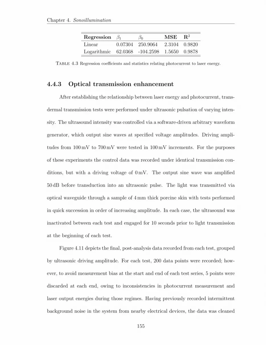
Chapter 4. Sonoillumination
Regression β1 β0 MSE R2
Linear 0.07304 250.9064 2.3104 0.9820
Logarithmic 62.0368 -104.2598 1.5650 0.9878
Table 4.3 Regression coefficients and statistics relating photocurrent to laser energy.
4.4.3 Optical transmission enhancement
After establishing the relationship between laser energy and photocurrent, trans-
dermal transmission tests were performed under ultrasonic pulsation of varying inten-
sity. The ultrasound intensity was controlled via a software-driven arbitrary waveform
generator, which output sine waves at specified voltage amplitudes. Driving ampli-
tudes from 100 mV to 700 mV were tested in 100 mV increments. For the purposes
of these experiments the control data was recorded under identical transmission con-
ditions, but with a driving voltage of 0 mV. The output sine wave was amplified
50 dB before transduction into an ultrasonic pulse. The light was transmitted via
optical waveguide through a sample of 4 mm thick porcine skin with tests performed
in quick succession in order of increasing amplitude. In each case, the ultrasound was
inactivated between each test and engaged for 10 seconds prior to light transmission
at the beginning of each test.
Figure 4.11 depicts the final, post-analysis data recorded from each test, grouped
by ultrasonic driving amplitude. For each test, 200 data points were recorded; how-
ever, to avoid measurement bias at the start and end of each test series, 5 points were
discarded at each end, owing to inconsistencies in photocurrent measurement and
laser output energies during those regimes. Having previously recorded intermittent
background noise in the system from nearby electrical devices, the data was cleaned
155

Chapter 4. Sonoillumination
Figure 4.11 The application of ultrasonic pulsation yielded distinct differences in mea-sured optical power with increasing driving amplitude until leveling off above 400mV, sug-gesting that there is an upper limit to the degree of tissue modulation that occurs underlow intensity pulsation.
for outliers, which occurred roughly every 12th data point, by identifying outlier in-
dices using normalized datasets. The normalized datasets were generated according
to Eq. 4.15, wherein P (x) represents the photocurrent at index x, whereas µn and
σn represent the relative means and standard deviations of the respective test.
N(x) =P (x)− µn
σn(4.15)
Outliers were defined as those points that occurred beyond the 90% confidence
interval established by µnorm ± 1.645σnorm, wherein µnorm and σnorm represent the
mean and standard deviation of the respective normalized datasets. Additionally,
156

Chapter 4. Sonoillumination
Figure 4.12 When scaled against the control mean value, increasing ultrasonic drivingamplitude improves the transmitted transdermal optical power by a maximum factor of1.742 times the control mean.
variation in laser intensity from between pulses coincided with significant deviations
in the photocurrent at corresponding indices. To account for this source of error,
the normalized laser energy was therefore scaled using the standard deviation of the
photocurrent, which was then subtracted from the photocurrent data.
The resultant data was translated into units of optical power based on the
logarithmic regression coefficients included in Table 4.3. The optical power data is
depicted in Figure 4.11, grouped by ultrasonic driving voltage. After observing the
significant change in transmitted optical power, the data was scaled by the mean of the
control sample to demonstrate the factor by which the optical power increased. Figure
4.12 depicts the mean improvement factor observed under each driving amplitude
157

Chapter 4. Sonoillumination
and demonstrates that low intensity ultrasound consistently increases optical power
with increasing ultrasonic amplitude. The maximum mean improvement factor was
recorded as 1.742 ± 0.0526 times the control mean under 400 mV driving voltage,
which plateaued to an average 1.733 ± 0.0549 times the control mean. The error bars
shown, which represent one standard deviation above and below the respective mean,
also confirm that improvement factors recorded at driving amplitudes beyond 400 mV
did not statistically differ from the maximum observed value. The full process of error
analysis was performed in MATLAB and is made available in Appendix C.
4.5 Discussion
This project hypothesized that the paraxial application of continuously pulsed
ultrasound and laser illumination would substantially modulate the optical proper-
ties of the local tissue such that an increase in total transmitted intensity might be
observed. In that regard, a calibration correlation was established to relate the mea-
surable photocurrent generated by light transmitted into a sealed integrating sphere
with the incident optical power upon the measurement device. Although theory had
predicted in an ideal setting that the relationship would be strictly linear, the data
shown in Figure 4.10 suggests that the improvised measurement system employed
in these experiments was only approximately linear for a short region, but became
increasingly less accurate beyond that region. Comparing the least-squares coeffi-
cients of the linear and logarithmic regressions, included in Table 4.3, revealed that
the log fit exhibited a smaller Mean Squared Error and a slightly higher coefficient
of determination, which confirmed that measuring the voltage drop across a series
158

Chapter 4. Sonoillumination
0.2 0.4 0.6 0.8 1 1.2 1.4 1.6 1.8 2−500
0
500
1000
1500
2000
2500
3000
Frequency (MHz)
RL
(Ohm
s)
Calculated Resistance vs Frequency (Impedance Matched)
510 kHz
1
0.2 0.4 0.6 0.8 1 1.2 1.4 1.6 1.8 2
−2000
−1500
−1000
−500
0
500
1000
Frequency (MHz)
XL
(Ohm
s)
Calculated Reactance vs Frequency (Impedance Matched)
510 kHz
1
Figure 4.13 After incorporating an L-match impedance matching circuit, the resistanceof the 500 kHz transducer dropped to 74.21 Ω while the reactance dropped to −51.65 Ω.
resistor did not permit the linear translation of photocurrent to optical power. The
method of measurement represented an indirect calculation of photocurrent, and so
necessitated the assumption that the imposition of the voltage probe upon the system
would negligibly affect the current measurement. However, should this assumption
not hold true, the system would likely behave somewhere between the original loga-
rithmic relationship and the ideal linear correlation, as was observed. Nevertheless,
recording the approximate photocurrent in this manner did result in a logarithmic
relationship that was less concave than measuring the photovoltage directly, which
was preferable for the purposes of these experiments.
With regard to transmitting the ultrasonic driving signals to the transducers,
electrical impedance matching circuits were designed and calculated by the data in-
cluded in table 4.2. After incorporating the impedance matching circuit, the effective
resistance of the circuit + transducer decreased from 89.01 Ω to 74.21 Ω while the reac-
tance decreased from −630.73 Ω to −51.65 Ω, as shown in Figure 4.13. These changes
159

Chapter 4. Sonoillumination
resulted in a total impedance magnitude of |Z| = 90.42 Ω, which although not ideal
was considerably closer to the goal 50 Ω impedance than the original impedance of
the transducer. The impedance magnitude spectra for both the 500 kHz transducer
on its own and the impedance matched transducer pair are included in Figure 4.14.
The plots demonstrate the drastic difference in impedance “seen” by the sine wave
transmitted from the RF amplifier toward the transducer and the importance of ap-
propriate impedance matching in electrical circuits.
However, the most appropriate method of realizing the impact of the impedance
matching circuit on the power transmission is using the source-load reflection coeffi-
cient, ΓSL, which can be calculated using equation 4.16 below, and provides a measure
of the portion of the the signal that will be reflected from the interface between two
circuits of differing impedance. The original reflection coefficient of the transducer
was 85.44% of the incident energy, which resulted in minimal acoustic generation
and significant losses in the system. The impedance-matched system, however, oper-
ated with a reflection coefficient of 28.79%, which permitted significantly more power
transmission and acoustic generation.
ΓSL =ZL − ZSZL + ZS
(4.16)
The RF amplifier incorporated two digital displays that provided a measure
of the power forward and power reflected from the circuit + transducer pair. This
data was recorded, however, the displays did not provide sufficient significant figures
to be of practical use in measurement. That being said, the average reflected power
160

Chapter 4. Sonoillumination
0.2 0.4 0.6 0.8 1 1.2 1.4 1.6 1.8 2
0
500
1000
1500
2000
2500
3000
Frequency (MHz)
Magnit
ude
(Ohm
s)
Magnitude Impedance Response (510 kHz)
510 kHz
1
0.2 0.4 0.6 0.8 1 1.2 1.4 1.6 1.8 2−500
0
500
1000
1500
2000
2500
3000
Frequency (MHz)
Magnit
ude
(Ohm
s)
Magnitude Impedance Response (Impedance Matched)
510 kHz
1
Figure 4.14 [Left] Plot of the impedance magnitude of the 500 kHz transducer. [Right]Plot of the impedance magnitude of the impedance-matched transducer. The matchingcircuit was designed to drag down the impedance of the transducer at the central frequencyof 510 kHz.
coefficient throughout the testing amounted to approximately 16.69%, which suggests
that the physical impedance matching circuit functioned better than the analysis
would have predicted based on the source-load reflectance coefficient calculated above.
However, it is worth noting that the method of impedance analysis only provided an
estimate, which is not to be equivalated to the analysis that could be provided by
a specialized RF impedance measurement device. This discrepancy may account for
the difference in analyzed performance as compared to the qualitative observations
regarding reflected power. Nevertheless, the impedance matching circuit allowed for
ample power transmission to generate acoustic pulses, to the point that under high
amplitude pulsation, the transducer was able to incite the generation of a column of
bubbles in water.
After calibrating the relationship between incident optical power and measured
photocurrent and more closely matching the effective electrical impedance, the ul-
161

Chapter 4. Sonoillumination
trasound modulation experiments revealed that increasing ultrasonic amplitude cor-
responded with a consistent improvement in transmitted optical intensity through
4 mm of porcine skin, consisting of epidermis, dermis, and adipose tissue. The data
in Figure 4.11 distinctly shows isolated increases in transmitted intensity as compared
to the control sample with no ultrasound applied. This data accounted for known
sources of error resultant from variations in laser energy between pulses, intermit-
tent high frequency interference from nearby electronics, and a wandering baseline
related to the exposed leads of the series resistor. In that regard, normalizing the
laser energy data determined the unitless relative deviance due to variations in pulse
output energy corresponding directly with peak photocurrent measurements of the
same point index. This data was scaled and deducted using the respective standard
deviation of the photocurrent to countermand the effect that fluctuations in output
laser intensity imparted upon the measured change in transmission. Additionally,
the margins of error were further reduced by the omission of outliers, which occurred
regularly every 12th data point as the result of a high frequency pulse interfering
with the signal. It is suspected that this pulse was associated with the cycling of
the pulsed power circuit driving the laser. Finally, observation of the difference in
normalized datasets revealed that the baseline intensity of the measurement probe
was not consistent throughout the tests. This phenomenon, commonly referred to as
a “wandering baseline” in the analysis of data from electrocardiograms (ECG’s), was
accounted for by means of deducting an 11-point moving average from the photocur-
rent, which stabilized the baseline while preserving the random measurement error
associated with the photodiode and variations in optical scattering and anisotropy.
162

Chapter 4. Sonoillumination
Pulsation Amplitude Mean Amplification Factor Standard Deviation
0 mV control 1.0 0.0306
100 mV 1.1813 0.0398
200 mV 1.4755 0.0400
300 mV 1.6607 0.0549
400 mV 1.7421 0.0526
500 mV 1.7261 0.0503
600 mV 1.7373 0.0613
700 mV 1.7298 0.0554
Table 4.4 Amplification factor statistics by ultrasonic driving amplitude
The resultant intensity data varies randomly throughout each individual test
group. This may also suggest that the duration of application was not an important
factor in amplifying the transmission, but was certainly indicative of its irrelevance for
durations less than 210 seconds. Moreover, the distinct jumps between test groups
are further indicative of an immediate response of the tissue to the application of
the ultrasound, as a delayed or prolonged response would have been observed in the
wandering baseline. This assertion could be confirmed in future experimentation by
comparing the application of ultrasound in order of both increasing and decreasing
intensities. Additionally, Figure 4.12 demonstrates that the increase in transmitted
intensity appears to approach an upper threshold. The amplified mean values are
included in Table 4.4 and reach a plateau around an average amplification factor of
1.733 ± 0.0549 times the control mean. Prior research into the mechanisms behind
UOT suggest that the changes in mass density and optical phase due to the periodic
compressions and rarefactions of tissue reduce scattering and permit a deeper pene-
tration depth into the tissue. However, it is reasonable to conclude that the tissue
may only be modulated so much before the application of ultrasound ceases to further
163

Chapter 4. Sonoillumination
alter tissue properties. Consequently, it is speculated that increasing the ultrasonic
amplitude beyond the observed values would likely not result in a measured deviation
from this plateau, until such point as the application resulted in a significant trans-
formation of the local tissue structure. For example, the application of high intensity
ultrasound may result in the cavitation of the local tissue by means of sonophoresis,
which may further alter the optical properties beyond the observed upper thresh-
old. Alternatively, operating at different frequencies may also vary the maximum
amplification factor, although a similar curve and plateau would be expected.
4.6 Conclusions and continued research
This series of experiments successfully confirmed the potential for ultrasonic
pulsation to be utilized to mechanically alter the optical properties of ex vivo tis-
sue, encouraging increased transdermal light transmission through porcine analogues
of human skin. With regard to potential applications, the increase also implies a
reduction in light either back-scattered or absorbed within the tissue, which would
permit a greater proportion of incident energy to be delivered to a clinical target
below the epidermis. The combination of two well-established clinical technologies in
this manner boasts the potential to both improve procedural efficacy and to reduce
the severity of detrimental side effects resultant from unwanted absorption by biolog-
ical chromophores, such as epidermal melanin. Moreover, the potential to effectively
bypass undesirable melanin absorption may allow for the expansion of light-based
procedures to patients of darker complexions.
Founding this mechanical tissue optical clearing technique on low intensity ultra-
164

Chapter 4. Sonoillumination
sound also offers the option to further improve the technique by either incorporating
chemical OCAs to further clear the tissue or otherwise increasing the ultrasound in-
tensity to induce cavitation within the tissue. Continued research into this technology
should investigate a spectrum of ultrasonic amplitudes and frequencies to more thor-
oughly establish tissue behavior throughout and beyond the intensities investigated
herein. Additionally, the project will investigate other design applications in order to
implement paraxial pulsation with traditional free space optical transmission devices
used in contemporary clinics while also investigating behavior under clinically rele-
vant laser energy levels. For example, refracting the ultrasound into the tissue using
a silicone elastomer wedge may permit application with free-space beams, but also
may operate at a sufficiently high angle of incidence to be beyond the aforementioned
threshold between GRIF operations. With regard to project specifics, future efforts
would do well to investigate:
• a continuous range of increasing ultrasonic amplitude to include amplitudes
sufficient to generate microcavities within the tissue, thereby effecting a physi-
ological change and potentially further improving forward transmission;
• differing incident angles for both the laser and acoustic propagation vectors to
characterize the regimes of GRIF operation;
• a variety of acoustic frequencies, particularly around the primary and secondary
thresholds tabulated in Table 4.1 by choosing a handful of different ultrasonic
transducers and generating acoustic waves throughout their central 6 dB band-
widths, to characterize the efficacy of sonoillumination by pulse frequency.
165

Chapter 5
Backward-mode waveguide-mediatedphotoacoustic tomography
Portions of this chapter have been reproduced with permission from the manuscripts
entitled Planar waveguide light transmission modality for backward-mode photoa-
coustic tomography, authored by Mason W. Schellenberg, Paul J.D. Whiteside, and
Heather K. Hunt, along with the Master’s Thesis entitled Photonic Ablation via Quan-
tum Tunneling authored by Paul J.D. Whiteside, Bioengineering Department, Uni-
versity of Missouri, May (2015) [66, 67].
5.1 Introduction
The field of photoacoustic tomography represents a significant divergence from
traditional acoustic technologies involving pulsed ultrasound, in that the acoustic
pressure waves are produced from within the medium, rather than applied to its sur-
face. Specifically, photoacoustics refers to the phenomenon wherein a short burst of
optical radiation generates a subsequent ultrasonic pulse through the rapid thermoe-
lastic expansion of an optical chromophore, such as a blood vessel or melanotic tumor
[174]. As such, photoacoustics has been utilized in a wide variety of applications
166

Chapter 5. Waveguide-mediated PAT
ranging from the detection of circulating tumor cells and blood oxygenation to the
evaluation and optical characterization of surfaces and thin films [62, 136, 144, 196–
198].
In typical photoacoustic applications, a laser beam of sufficiently short pulse
duration is absorbed by an optical chromophore, causing the absorber to undergo
a rapid thermoelastic expansion, which generates an ultrasonic pressure wave that
propagates throughout the medium. Much like traditional ultrasound, these acoustic
waves carry information about the underlying tissue structure and may be recorded
and analyzed to determine the depth of a single acoustic source or to generate a 2D
or 3D tomographical map of the tissue structure [60, 174]. However, unlike tradi-
tional ultrasound, the acoustic information is based on the optical properties of the
medium rather than acoustic differences between tissues [159]. This distinction per-
mits the imaging of acoustically similar tissues based on differences in relative optical
properties. For example, Zhang et al. have used photoacoustics to reconstruct 3D
tomographical maps of the in vivo vasculature of mouse models, relying on the strong
optical absorption of hemoglobin as compared to the surrounding dermal tissues [199].
Such structures are typically unresolvable by traditional ultrasonics, as those tech-
niques predominantly rely on differing material properties, such as compressibility,
density, and acoustic impedance, to resolve the boundaries of interfacing materials,
such as bone and soft tissue [200, 201].
However, despite providing useful and relevant information regarding previously
unresolvable structures, photoacoustic tomography has seen limited clinical imple-
mentation owing to the necessity for the technique to be performed in “backward
167

Chapter 5. Waveguide-mediated PAT
mode.” This backward mode of operation refers to the parameter wherein the ultra-
sonic pressure waves must be detected on the optically irradiated side of the tissue,
due to the potential interference of echogenic structures, such as bone or lung tissue,
and the reduction in signal to noise ratio (SNR) associated with acoustic attenuation
through acoustically anisotropic tissues [63].
Typical ultrasonic detectors utilized in both ultrasonic tomography and labo-
ratory photoacoustics are based on piezoelectric elements, which are cheap to man-
ufacture and can be constructed in a wide range of configurations from large low
frequency individual elements to high frequency linear or matrix arrays. However,
problems in backward mode photoacoustics arise, because piezoelectric materials are
typically opaque and therefore complicate the laser irradiation component of the
backward mode design by occluding the path of the light when applied coaxially.
This has led to the development of three prevailing solutions: (1) to design acoustic
detectors that incorporate through-holes to permit coaxial optical fiber radiation of
tissue, (2) to spatially separate the acoustic detector from the tissue using a trans-
parent acoustic couplant to transmit light at an angle to the tissue surface, or (3)
to use complex dual-wavelength optical detection systems to irradiate tissue through
dichroic coatings [63, 159, 202].
Whereas each of these methods has shown promise, each also incorporates addi-
tional challenges. For example, when incorporating a cavity through which an optical
fiber may irradiate the tissue, the through-hole necessitates changes to the surface
detection geometry of the transducer. This alteration from a “disk” to a “ring” ge-
ometry introduces an additional edge near the center of the transducer, which can
168

Chapter 5. Waveguide-mediated PAT
subsequently introduce acoustic ringing in the detected signal. The ringing effect
may also introduce acoustic artifacts and overwhelm otherwise valuable information,
causing a decrease in SNR and a loss of resolution; accordingly, this solution has
not seen much development outside of some initial investigations by the Viator lab-
oratory. With regard to the second solution, however, the spatial distancing of the
detector from the tissue surface increases acoustic attenuation and signal loss, while
also allowing acoustic signals to reflect within the detection chamber, both of which
can also decrease SNR. The third solution does not experience such problems, as the
opaque transducer is replaced with a dichroic-based optical detector. Such systems
use two lasers simultaneously, one to generate photoacoustic pulses by transmitting
through the dichroic cavity, and the other to scan and detect changes to the geome-
try of the cavity resultant from acoustic pressure variations [60, 63]. These systems
can demonstrate remarkable resolution, as the detection surface is strongly correlated
with the spot size of the interrogating beam and the translational resolution of the
scanning stage or deformable mirror. However, such systems require two separate
lasers along with complex optical components that necessitate rigid, reliable align-
ment of both incident beams. Although these systems produce exceptionally accurate
reconstructions and can be used for in vivo analysis in backward mode, due to their
complexity they are often ill-suited for portable clinical applications.
5.2 Technical discussion
This project represents an alternative solution to the backward mode paradigm,
using a planar selective release waveguide to irradiate the tissue directly underneath
169

Chapter 5. Waveguide-mediated PAT
the detection surface of an ultrasonic transducer or transducer array. The principal
benefit of this modality lies in its ability to utilize readily available acoustic detection
equipment and software that are calibrated for use with piezoelectric elements, which
greatly simplifies any potential commercial and clinical applications of the technology
as compared to more complex approaches. The following sections describe the fun-
damental science behind photoacoustic signal generation and our proposed method
of photoacoustic tomography.
5.2.1 Photoacoustics
As discussed above, photoacoustics is the result of the rapid irradiation of an op-
tically absorbing particle by a short pulse of light. This photo-mechanical effect may
accompany the thermal expansion of any chromophore following a pulse of optical
irradiation; however, the resultant acoustic pressure wave is only useful for photoa-
coustic tomography in the event that two conditions are met. The first condition,
known as “stress confinement,” stipulates that the pulse duration of the incident laser
light must be shorter than the time required for the resultant acoustic wave to depart.
The condition for stress confinement is shown in Equation 5.1 below:
τ ≤ δ
cs(5.1)
wherein τ is the laser pulse duration, cs is the speed of sound in the medium, and
δ = 1/µa, where µa is the optical absorption coefficient of the target [144]. The second
condition, known as “thermal confinement,” necessitates that the energy absorbed by
170

Chapter 5. Waveguide-mediated PAT
the chromophore must not be dissipated in the form of heat before the acoustic wave
can depart. When firing a laser with a pulse width on the order of a few nanoseconds,
the heat dissipation away from the absorber may be neglected and all of the incident
electromagnetic energy is translated into acoustic pressure [203]. This pressure wave
can be described mathematically by Equation 5.2 below:
p(x, t) =1
2ΓgµaHBe
−µa(x−cst) +1
2ΓgµaHBe
−µa(x+cst) (5.2)
wherein Γg represents the Grunesian coefficient, HB is the radiant exposure of the
beam, x is depth, and t is time [204, 205]. At the surface of an ultrasonic detector,
where x = 0, the equation describes the recorded amplitude of the pressure wave
as a function of time. As the wave approaches the detector surface, the pressure
exponentially increases in amplitude followed by an immediate drop when the wave
hits the detector. Then, while the inverted negative pressure wave is reflecting away
from the detector, the recorded pressure follows a reciprocal exponential return to
the baseline. Peak-to-peak analysis is often used in photoacoustic experimentation,
as a result of this characteristic waveform profile observed by the detector.
5.2.2 Backward-mode transmission modality
Following the principles of photoacoustic signal generation, the majority of pho-
toacoustic systems use pulsed lasers operating with pulse widths on the order of a
few nanoseconds or less. A typical laser system for photoacoustic tomography is the
Q-Switched Nd:YAG laser, which generates a primary beam at 1064 nm, but whose
171

Chapter 5. Waveguide-mediated PAT
Figure 5.1 Transmitting the light through an off-axis waveguide in contact with thetissue allows the incorporation of a standard off-the-shelf transducer on the rear face todetect ultrasonic photoacoustic signals.
secondary harmonic is 532 nm, which is strongly absorbed by biological chromophores
such as hemoglobin and melanin. Moreover, some systems utilize the third harmonic
at 355 nm to drive an optical parametric oscillator (OPO), which allows the laser to
output pulses at wavelengths throughout the visible spectrum.
The system designed herein transmits the secondary harmonic of a Q-Switched
Nd:YAG laser into the tissue using a planar selective release waveguide (SRW) in
a manner similar to that discussed in the previous chapter. As the light transmits
along the SRW, it is contained within the silver cladding layer until it reaches the
designated active area, as shown in Figure 5.1. The light then transmits out through
172

Chapter 5. Waveguide-mediated PAT
the active area into the target medium, which for our purposes is skin tissue, and is
absorbed by an optical chromophore. As mentioned above, the short pulse width of
the laser generates an acoustic pressure wave whose properties are dependent upon
the optical characteristics of the chromophore. This pressure wave propagates up
through the tissue, across the SRW, and is detected by the transducer on the rear
face of the waveguide.
Unlike some competing systems, this design makes use of a standard piezoelec-
tric transducer element acoustically coupled to the rear face of the SRW. This orienta-
tion necessitates that the optical and acoustic characteristics of the SRW be balanced
to allow for transmission of the light into the tissue while also permitting the acoustic
energy to transmit across the waveguide substrate. For the purposes of these exper-
iments, our waveguides were made from a single sheet of poly-methyl methacrylate
(PMMA), which is largely transmissive to visible light and whose acoustic impedance
(ZPMMA = 3.26 MRayl) does not substantially differ from that of tissue (Zskin =
1.99 MRayl). The SRW substrates used in Chapter 3 were composed of fused silica
(ZFS =13.1 MRayl), which prevented sufficient transmission of acoustic energy due
to the significant acoustic impedance mismatch. The acoustic reflection coefficient at
the interface between any two media of differing impedances can be represented as:
R =
(Z2 − Z1
Z2 + Z1
)2
(5.3)
wherein Z1 and Z2 represent the incident medium and the external medium respect-
fully. That being the case, the reflection coefficient for an FS–tissue interface would be
173

Chapter 5. Waveguide-mediated PAT
approximately 0.542, whereas for a PMMA–tissue interface, the reflection coefficient
would be approximately 0.0585, which is an order of magnitude more transmissive.
We had briefly considered using an acoustic impedance matching layer with the fused
silica substrates, however, the available polymers that would have achieved greater
acoustic transmission would also have inhibited optical transmission into the tissue
by promoting total internal reflection instead. Future designs of the waveguide that
operate as planar beam deflectors, which will be discussed later on, may incorporate
acoustic matching layers, as they do not operate under the same internal reflection
conditions.
5.2.3 Technical objectives
Having previously established that collimated light could successfully be trans-
mitted into phantoms simulating human skin through direct contact, this project
represented a significant potential application that incorporated an auxiliary sensing
technology alongside laser irradiation. This sought to formally establish the poten-
tial for using planar waveguide irradiation as a means of achieving backward-mode
photoacoustic detection. As such, the primary milestone was pragmatic in that exper-
iments were designed to detect and analyze a simple one dimensional photoacoustic
signal measured with a 10 MHz transducer to correspond peak locations with known
chromophores. Following that, the technology was expanded to detect and analyze a
two-dimensional array of time-resolved photoacoustic traces to reconstruct a map of
photoacoustic sources. Accordingly, the goals of this project were as follows:
• Record photoacoustic signals in backward mode using a transducer on the rear
174

Chapter 5. Waveguide-mediated PAT
face of a waveguide and correlate with known chromophore depths;
• Design and fabricate a stand-alone signal multiplexer, incorporating printedcircuit boards to multiplex 32 input signals onto 4 oscilloscope channels;
• Record time-resolved photoacoustic data from 32 transducer elements in rapidsuccession by programming an automated LabVIEW VI;
• Reconstruct a 2D depth profile of a tissue phantom or ex vivo tissue sample inMATLAB using the k-space reconstruction methods.
5.3 Materials and methods
The following sections describe the procedures involved in waveguide fabrica-
tion and tissue sample preparation, along with a description of the optical apparatus
employed and the electronic instrumentation components and procedures. The exper-
iments discussed herein represent two distinct phases of development: (1) empirically
establishing the technique by recording preliminary photoacoustic data in a backward
mode, and (2) revising the apparatus to record data in a linear array and thereby
generate a two-dimensional profile.
5.3.1 Porcine tissue preparation
The porcine tissue samples for the preliminary research were prepared accord-
ing to the same protocols designed for aforementioned sonoillumination experiments.
Included for ease of reference, large sections of ex vivo porcine skin were donated for
this research project from the Mizzou Meat Market (College of Agriculture, Food, and
Natural Resources at the University of Missouri). The skin was disinfected in a 1.75%
ethanol solution for 2 minutes prior to processing for experimentation. Following dis-
infection, the sections were trimmed down to a thickness of 4 mm, incorporating
epidermal, dermal, and adipose tissue, and cut into 40 mm square samples. Orig-
inally, each sample was held taut and adhered at the edges with superglue over a
thin fiberglass mesh to individual 3D-printed tissue mounts, as shown in Figure 4.4,
175

Chapter 5. Waveguide-mediated PAT
which incorporated open apertures to allow for measurement of optical transmission
through the tissue. The fiberglass mesh was included to provide additional support
to the porcine skin and prevent potential indentation of the tissue during testing.
Processed skin samples were wrapped in moist Kim wipes to prevent dehydration,
enclosed in air-tight plastic bags, and stored in a freezer at 4°C until needed. Prior
to use, samples were defrosted by running water over the plastic bag for 10 – 15 min.
5.3.2 Turbid tissue phantom design
Due to the complexity and variability of biological tissues, while developing
the 2D photoacoustic imaging modality, optical tissue phantoms were utilized as a
controllable substitute for skin. The preparation protocol, adapted from procedures
published by Chen et al. , is based on a mixture of intralipid, methanol, agar, and
gelatin to generate an optically scattering gel with a speed of sound comparable to that
observed in tissue [206]. This procedure was refined through photoacoustic analysis
to closely match the speed of sound in test samples with the reported speed of sound
in tissue. Samples were produced by heating 13.73 mL of ultra-pure DI water to 30°C,
mixing the solution using a magnetic stir bar at 350 rpm, and then adding 5.472 mL
of 20% Intralipid, 2.94 mL of methanol, and 17.6 µL Formaldehyde 37%. After the
solution is homogenized, the mixing speed was increased to 700 rpm at which point
1.54 g of gelatin (300 Bloom) and 190 mg of agar were slowly added to the solution,
such that the powder did not aggregate in the solution. The beaker was covered
with an aluminum heat shield and was slowly heated up to 45°C. Once reached, the
solution was poured into a tissue phantom mold, which was then transferred into a
vacuum desiccator for 10 min to remove dissolved gas from the solution and minimize
the occurrence of air pockets. The mold was then placed in a 4°C refrigerator for 1
day to allow the solution to set.
176

Chapter 5. Waveguide-mediated PAT
Figure 5.2 [Left] The original design for the photoacoustic waveguides utilized PMMAsubstrates clad in silver and titanium; [Right] the active area of the waveguides exposedthe bare substrate, relying on silver to confine the light elsewhere within the waveguide,which was later revealed to provide a source of error owing to photoacoustic signals incitedwithin the metal cladding [67].
5.3.3 Waveguide fabrication
The original waveguides for this project were fabricated from 1.5 mm thick sheets
of PMMA (Evonik CRYO, 0A000 GT). This material was chosen for its relatively
low acoustic impedance, given that it is commercially available in transparent slabs.
There are other materials that would have resulted in a closer acoustic impedance
match to skin (Zskin = 1.99 MRayl; Zacrylic = 3.26 MRayl); however, few of them are
transparent at 532 nm or available in rigid planar sheets [207, 208]. Two different
waveguide designs were utilized for these experiments, with the second representing
a revision of the first following the results of preliminary testing. The original waveg-
uides were similar to those fabricated in Chapter 3, in that they were planar slabs
coated in titanium and silver with 45° polished entrance apertures, as depicted in Fig-
ure 5.2. The substrates were fabricated in-house to be 15 mm square units, cutting a
bevel at 45° and polishing the bevel with increasing grit optical sandpaper, finally fol-
lowed by a fine scratch removing compound specifically formulated for plastics (Novus
177

Chapter 5. Waveguide-mediated PAT
Fine Scratch Remover No.2). The two angled entrance and exit apertures of the sub-
strates were masked off with Kapton tape, along with a 9 mm x 15 mm rectangular
section of the largest face 3 mm from each end, which would serve as the waveguide’s
active area. The substrates were then clad in thin films of titanium and silver using a
cold sputtering vacuum deposition system (Quorum Technologies, K575X) to serve as
mirrors on the bounding surfaces of the substrate. The titanium was deposited using
a 99.998% pure Ti target at 90 mA for 60 s, which formed a film less than 10 nm thick.
The titanium acted as an adhesion layer for the silver, which was deposited from a
99.95% pure Ag target at 30 mA for 300 s to form a much thicker layer approximately
200 nm thick. Laser light incident perpendicularly upon one of the angled faces would
internally reflect along the waveguide to the exit aperture when exposed to air, but
would transmit out through the active area when in contact with tissue.
The results of our preliminary testing, which will be discussed in the sections to
follow, revealed that cladding the waveguides in silver incorporated significant noise
into the photoacoustic signals owing to a photoacoustic response incited within the
metal cladding. Consequently, for the continued experiments, the waveguide was
redesigned such that it did not incorporate an optically absorbing cladding. The
new waveguides have been revised such that they are comprised of two acrylic slabs
fused together using Norland Optical Adhesive 13685 (NOA 13685). This adhesive
was chosen based on its reported refractive index of n = 1.3685, such that light
incident at 45° within the acrylic substrates (n = 1.4937) would internally reflect
from the interface and be directed perpendicularly into the tissue. In this manner,
the waveguide behaves as a planar optical beam deflector, rather than a traditional
multiply-reflecting waveguide. However, at the moment, the fabrication protocols for
the new waveguide design are still under development and revision, so this section
will be revised following the completion of that design.
178

Chapter 5. Waveguide-mediated PAT
Figure 5.3 The optical apparatus was similar to previous systems, transmitting lightthrough a beamsplitter to trigger data collection and measure laser pulse energy, com-pressing the beam along one axis using an anamorphic prism pair, re-collimating the beam,and transmitting light through an SRW with an ultrasonic transducer on the rear face.
5.3.4 Experimental apparatus
The experimental apparatus involved a number of custom designed and fabri-
cated materials and circuits, in addition to standard optical components and elec-
tronic instrumentation. These materials and systems were revised between the two
phases of research to account for revelations and updated operating conditions. Ac-
cordingly, the sections that follow describe each of these components in detail.
5.3.4.1 Optical apparatus
The first phase of the project was intended to demonstrate backward-mode pho-
toacoustics with simple one dimensional generation and detection of photoacoustic
waveforms in porcine skin. As such, the optical apparatus was markedly similar to
those discussed in previous chapters, with some slight discrepancies, as shown in Fig-
ure 5.3. The light from a pulsed Nd:YAG laser transmitted first through a zero-order
half-waveplate (Thorlabs, WPH05M-532) and polarizing beamsplitter cube (Thor-
labs, CM1-PBS251). Rotating the waveplate rotates the incident linear polarization
with respect to the cube, resulting in what is known as a “variable beam splitter,” in
179

Chapter 5. Waveguide-mediated PAT
Figure 5.4 The waveguide and 10 MHz ultrasonic transducer were incorporated into asingle removable 3D printed cartridge that incorporated both components and a cavityfilled with ultrasound gel to transmit the photoacoustic signals.
that the rotation angle of the waveplate determines the relative portion of s- and p-
polarized light that either deflects toward the energy meter or transmits toward the
waveguide.
The light that is deflected is used to trigger data collection by generating a
photovoltage pulse using a high-speed photodiode (Thorlabs, DET10A), which was
chosen for its exceptionally fast rise time of 1 ns and sensitivity at 532 nm. The
light that transmits toward the waveguide also transmits through a 50:50 beamsplit-
ter cube, which directs half of the intensity toward a pulse power meter (Thorlabs,
PM100USB), which measures the pulse energy of the laser to account for variations
in intensity between pulses. The other half of the energy transmits through a 4X
anamorphic prism pair (Thorlabs, PS883-A), which double refracts the beam be-
tween two fixed-angle prisms and thereby compressed the beam along one axis to
transform the beam from a circular Gaussian profile into an elliptical Gaussian ap-
proximately 1.5 mm thick along its narrow axis. The extreme degree of compression
resulted in significant dispersive effects, which were corrected using a long focus cylin-
drical lens (Thorlabs, LJ1558L2-A), which re-collimated the beam prior to entering
the waveguide.
The waveguides were fabricated as described in the previous section and were
180

Chapter 5. Waveguide-mediated PAT
fixed at a 45° incline with respect to the incident beam using a custom 3D printed
optomechanical mount, as shown in Figure 5.4. That was rigidly connected to the op-
tical train. Unlike the apparatuses discussed in previous chapters, these experiments
did not necessitate an integrating sphere, as we were not measuring transmitted op-
tical intensity. The light transmitted out of the waveguides into the porcine tissue
samples, which had ABS plastic absorbers embedded into the dermis to simulate bi-
ological chromophores at an appropriate depth. The second phase of this project is
currently under development, but is intended to make use of tissue phantoms with
tubes filled with an artificial blood analogue to properly characterize the 2D photoa-
coustic tomography system prior to conducting experiments on ex vivo tissue.
5.3.4.2 Electronic apparatus
The goal of these experiments was to establish a backward-mode method of perform-
ing photoacoustic tomography in tissue phantoms and samples with distinct relevance
to empirically mapping the severity of thermal injuries. Accordingly, pulsed laser
light, generated by a Q-switched Nd:YAG laser (Opotek, Vibrant 355 II) operated
at a wavelength of 532 nm with a 5 ns pulse width, was transmitted through porcine
skin samples. Optical chromophores consisting of a Direct Red dye solution in trans-
parent tubing absorbed the light and generated photoacoustic pulses. These pulses
were detected by a custom-ordered 32 channel ultrasonic transducer array, which op-
erated with a 12.5 MHz ± 10% central frequency. The array was designed to utilize
a −6 dB bandwidth of 60% extending from roughly 7.5 MHz to 17.5 MHz. Elements
were 0.15 mm wide, with an element pitch of 0.20 mm, an inter element spacing of
0.05 mm, and an element width of 6 mm. The total active dimensions for the 32
consecutive rectangular elements was 6.35 mm x 6 mm. The array was acoustically
impedance matched to PMMA (roughly 3.3 MRayl) to minimize reflections at the
interface with the waveguide. Finally, the array operated under a stated 50 Ω output
181

Chapter 5. Waveguide-mediated PAT
impedance; however, the specifications documentation provided by the manufacturer
states “Imasonic designs its phased array probes to get real impedance as close as
possible to 50 Ω... the real impedance is higher than 100 Ω. The capacitive imaginary
part is typically not matched.”
As described above, the transducer array was connected to a custom-designed
32 channel multiplexer, described in the next section, which amplified four output
signals simultaneously, while shunting the unused signals to ground. The output
signals of the multiplexer were indexed by an Arduino Mega R3, which received
indexing commands via LabVIEW serial output through a USB cable. For any one
full 32-element image to be generated, a minimum of 8 laser pulses were required. The
output channels of the multiplexer were fed via BNC cable to the four input channels
of the Picoscope 5442B USB oscilloscope, incorporating 50 Ω feed-through terminators
to minimize reflections in the lines due to electrical impedance mismatching. Laser
pulses, controlled by LabVIEW via RS-232 commands, triggered data collection by
irradiating a photodiode (Thorlabs, DET 10A).
A LabVIEW automation software was designed to control laser operations, mul-
tiplexer indexing, and data acquisition. The software was programmed to index the
multiplexer outputs onto their first input channel, fire a single pulse of the laser,
trigger data collection, record the laser pulse energy, and save the waveform to a file.
Following that procedure, the next multiplexer input channel was indexed and the
process was repeated. Image processing was performed in MATLAB using the k-wave
toolbox (Available from www.k-wave.org, maintained by Bradley Treeby, Ben Cox,
and Jiri Jaros) [209, 210].
5.3.4.3 Multiplexer design
In order to obtain higher quality imaging resolution in the second phase of the project,
a 32 channel linear array transducer was custom manufactured by Imasonic (Imasonic
182

Chapter 5. Waveguide-mediated PAT
Figure 5.5 [Top] The geometry of the array transducer is such that there are 32 elementswith rectangular detection areas h x (p - e); [Bottom] the array transducer is incorporatedinto a stainless steel housing with a footprint comparable to the rear face of the standardSRW used in these studies.
SAS, Voray-sur-l’Ognon, France). The linear array was manufactured with a central
frequency of 12.5 MHz. Each of the 32 contact areas were designed with an element
width of h =6 mm, an element pitch of p =0.20 mm, and an element spacing of
e =0.05 mm for a total active area length of l =6.35 mm, as shown in Figure 5.5. The
array was also acoustically impedance matched to PMMA (3.3 MRayl).
However, given the necessity that each of the 32 channels be recorded individu-
ally to preserve signal integrity between channels, and given that the USB oscilloscope
(Picoscope 5442B) being utilized was only equipped with 4 channel inputs, a 32 chan-
nel multiplexer was required to achieve optimal photoacoustic tomography. Investiga-
tions into commercially available multiplexers capable of accepting signals within the
appropriate frequency bandwidth exclusively yielded options beyond the limitations
of the available grant budget. A thorough literature search revealed that Gamelin
183

Chapter 5. Waveguide-mediated PAT
et al. had developed such a multiplexer for photoacoustic tomography in-house us-
ing commercially available electronics components; whereas Gamelin did not provide
the circuit diagrams for their proprietary multiplexer, the manuscript listed the part
numbers of each of the primary components, including the appropriate operational
amplifier chips (op-amps) and the 8-channel multiplexer (mux) chips [211].
Using Gamelin et al. as a foundation, it was determined that the 32 channels
would be best multiplexed onto the 4 BNC input channels of the oscilloscope using
four individual 8-channel multiplexer boards, which would accept 8 input signals,
amplify and output the desired signal to a 50 Ω impedance BNC cable, and shunt
the other 7 to ground to reduce cross-talk between signals. However, it was fur-
ther determined that constructing each of these multiplexer boards using standard
through-hole breadboards and wiring would invite excessive external interference and
exacerbate signal decomposition. Accordingly, an 8-channel multiplexer circuit was
designed as a printed circuit board (PCB) using AutoDesk Eagle PCB software and
ordered from Advanced Circuits. Five boards were ordered from Advanced Circuits,
allowing for one “practice” board, given the exceedingly small size of some of the
chosen components.
Figure 5.6 depicts the AutoDesk EagleCAD design of a single 8-channel mul-
tiplexer board, with red components representing the top routes, blue representing
the bottom, and green representing the soldering pads. The circuit is designed to
accept unregulated ± 7.5 V and ground input on the left side of the board. The
7.5 V unregulated power supply fed a 5 V Low-Dropout regulator (LDO), which was
stabilized by the capacitors in positions C2, C3, C6, and C7, whose values are listed
in Table 5.1, in addition to the diodes in positions D1 and D4. Similarly, the −7.5 V
unregulated power supply fed a −5 V LDO, which was stabilized by the capacitors in
positions C4, C5, C6, and C7 along with the diodes in positions D2 and D3. These
two LDO circuits provided ±5 V regulated power to the op-amps and mux chips.
184

Chapter 5. Waveguide-mediated PAT
42DON'T PANICDON'T PANIC
Figure 5.6 The multiplexer boards were designed to accept 8 signal inputs, to amplifyand output 1 signal, and to shunt the other 7 to ground to reduce cross-talk between signals.The signals were input via two ribbon cable ports at the top and bottom, whereas powerwas provided via the three pin port on the left, and the multiplexer logic commands wereprovided from the three pin input port on the right.
The boards were designed to accept four input signals from the Imasonic array
transducer at the top and bottom of the layout. Each of the signals was fed to
an independent op-amp, which was designed as a non-inverting high-gain amplifier to
improve the signal-to-noise ratio (SNR). The gain was defined by the ratio of resistors
R1 and R4, which were the feedback (Rf ) and input (Ri) resistors, respectively. The
gain equation for such a non-inverting amplifier is shown in Equation 5.4 below:
G = 1 +Rf
Ri
(5.4)
185

Chapter 5. Waveguide-mediated PAT
Figure 5.7 Stackable multiplexer boards were designed in EagleCAD to minimize highfrequency interference, and were then printed by Advanced Circuits, LLC. The words ofadvice in the bottom left corner of the board are actually etched in copper as well andserve to aid the manufacturer in discerning between the files for the front and rear circuittraces.
As such, the gain could be set to either G = 20 or G = 10, depending on
the choice of R4. It should be noted that the op-amp becomes less stable at high
gains for higher frequency signals, so a lower gain should be selected if excessive
ringing is observed in the output signal. Moreover, gains lower than 10 necessitate
the incorporation of a compensation circuit, which may consist of a single capacitor
or a capacitor and a resistor in series. The data sheet for the op-amps used for
these multiplexer circuits recommended a compensation capacitor of 15 pF for a gain
of 10, but did not require anything to be connected to the circuit for a gain of
20. Additionally, these particular op-amps incorporated a “disable” pin, which when
deactivated would route the input signal to ground to minimize cross-talk between
amplified signal channels within the mux chips. The op-amps and mux chips were
all independently stabilized on both their positive and negative supply rails using
186

Chapter 5. Waveguide-mediated PAT
Symbol Description Manufacturer Part Number Footprint
LDO +5V 5 V supply AZ2940D-5.0TRE1 TO-252-3
LDO -5V −5 V supply LM2990SX-5.0/NOPB TO-263-3
MUX-SIG Signal output selection MAX4051ESE+ 16-SOIC
MUX-DIS Disabling signals MAX4051ESE+ 16-SOIC
OP(#) High gain op-amps AD8099ARDZ-REEL7 8-SOIC
D(#) Diodes RS3AB-13-F DO-214AA
C1 100 pF CL05C101JC51PNC 0402
C2 0.1µF GRM155R62A104KE14D 0402
C3 0.33µF CL31B334KBFNNNE 1206
C4 1.0µF CL31B105KCHNNNE 1206
C5 2.2µF HMK316ABJ225KL-TE 1206
C6 10µF UMK316BBJ106ML-T 1206
C7 47µF C3216X5R1E476M160AC 1206
R1 499 Ω RC1206FR-07499RL 1206
R2 49.9 Ω RC1206FR-0749R9L 1206
R3 1 kΩ RC1206FR-071KL 1206
R4 (G=20) 26.1 Ω RC1206FR-0726R1L 1206
R4 (G=10) 53.6 Ω ERJ-8ENF53R6V 1206
SMB Molex right angle SMB 731000103 SMB
Table 5.1 This table lists each of the components utilized in the creation of the 8-channelmultiplexer PCB’s shown in Figure 5.6. All components were purchased on Digikey.com
capacitors C1 and C2.
The output pins of each op-amp were fed to the 8-channel mux chip labeled
“MUX-SIG,” whereas their respective disable pins were fed to the mux chip labeled
“MUX-DIS.” The two mux chips were indexed by the three input pins labeled ADDA,
ADDB, and ADDC. These digital indexes simultaneously controlled the output of
MUX-SIG while also disabling the op-amps for each of the 7 unused signals through
MUX-DIS. The digital address pins were the final input on the right side of the
board and were designed for this case to be operated by an Arduino Mega 2560
microcontroller, which would in turn be operated by USB output from a LabVIEW
automation software. Finally, the output of MUX-SIG was directed to a 50 Ω output
impedance Molex SMB right-angle connector.
187

Chapter 5. Waveguide-mediated PAT
Figure 5.8 The assembled multiplexer boards are stacked and fed unregulated ± 8 Vand ground, 8 signal inputs each, and 3 arduino address signals. The multiplexed signalsare output via SMB connectors to BNC front-panel ports, which then feed to the 4 inputchannels of the Picoscope 5442B, including 50 Ω feedthrough terminators on each channelto minimize reflections.
Using four of these boards stacked on top of each other, as shown in Figure
5.8, the 32 channels of the array transducer were separated into groups of 8, isolated,
amplified, and output to one of the four BNC input channels of the oscilloscope.
Signals (1–8) corresponded to Channel A, (9–16) to Channel B, (17–24) to Channel
C, and (25–32) to Channel D. Additionally, each of the BNC channels incorporated a
50 Ω feedthrough terminator to more appropriately match the electrical impedance.
5.4 Results
As discussed previously, this project proceeded in two distinct phases, the first
of which was intended to demonstrate proof of concept to show that backward-mode
photoacoustics could be performed using selective release waveguides, whereas the
second was intended to improve upon that system to generate a 2D depth profiling
188

Chapter 5. Waveguide-mediated PAT
system for tomographic applications in a clinical setting. The first phase utilized
porcine skin samples embedded with ABS plastic chromophores and demonstrates
1D photoacoustic depth profiling. The second phase utilized tissue phantoms that
were specifically designed to be both optically and acoustically analogous to tissue,
while permitting strong control over the position and depth of blood vessel analogues.
5.4.1 Preliminary results
To establish the groundwork for a backward-mode waveguide-based photoacous-
tic tomography modality, the initial phase of the project involved the generation and
detection of photoacoustic signals within ex vivo samples of porcine skin, detecting
the ultrasonic pulses on the reverse face of the transmitting waveguide. In that re-
gard, experiments were designed such that the laser was fired 16 consecutive times,
resulting in 16 waveforms that were averaged to improve signal to noise ratio (SNR).
The light was transmitted into two tissue samples, one consisting of the original
porcine tissue and the other consisting of porcine tissue with an ABS black plastic
chromophore embedded in the back side of the dermis. The waveforms generated
within each sample were compared to identify the sources of individual peaks and
confirm that the signals from the ABS plastic chromophore could be successfully iso-
lated and identified. To accomplish this, the position of each peak in the time domain
was recorded and matched to the time of flight predictions based on the various paths
and reflections that it might have taken, utilizing the speeds of sound in each of the
materials involved (cacrylic =2730 m/s; cgel ≡ cwater =1570 m/s; cskin =1595 m/s) to
additively determine the total time of flight for each peak [206–208].
Figure 5.9 depicts the photoacoustic trace of the ABS-implanted tissue sample,
and demonstrates the occurrence of six events of interest. The first two positive
peaks, occurring at 3.942 µs and 4.026 µs were the closest to the transducer face and
were determined to correlate with internal reflection points within the waveguide,
189

Chapter 5. Waveguide-mediated PAT
4 4.5 5 5.5 6 6.5 7 7.5 8 8.5−300
−250
−200
−150
−100
−50
0
50
100
150
200
Time [ us ]
Am
plitu
de [
mV
]
Photoacoustic trace detected from porcine tissue in backward mode
Student Version of MATLAB
Figure 5.9 The photoacoustic peaks were analyzed to reveal that the most significantpeaks were resultant from optical absorption by the silver cladding, which also generatedacoustic reflections; these observations provided justification to redesign waveguide fabri-cation protocols to avoid using optically absorbing cladding layers.
suggesting that the silver cladding was producing a photoacoustic response. The two
negative peaks occurring at 5.102 µs and 5.192 µs represent the reflections of these
signals from the waveguide tissue interface. Finally, the peaks occurring at 5.62 µs
and 7.86 µs correspond strongly with the known position of the ABS chromophore.
Additionally, although the former peaks were present in the traces recorded from the
unaltered porcine skin sample, the latter peaks were not, contributing to the assertion
that these peaks were the result of optical absorption by the ABS chromophore.
5.4.2 2D Depth Profiling
Having empirically proven that the backward mode technique to be a viable
method of both transmitting light into ex vivo tissue and detecting the subsequent
190

Chapter 5. Waveguide-mediated PAT
ultrasound, the project advanced to the second phase, wherein the single element
transducer would be replaced by a 2D array of piezoelectric elements. Owing to the
increased complexity of the acoustic apparatus, the initial 2D photoacoustic tomog-
raphy experiments were designed to be performed first on well-controlled artificial
tissue phantoms. The fabrication protocols for establishing appropriate phantoms to
use in developing a bespoke photoacoustic imaging modality were refined experimen-
tally to accurately replicate reported values of the speed of sound in tissues while also
replicating appropriate optical scattering.
Although the tissue phantoms were designed based on a protocol published
by Chen et al. , reproducing the protocol did not precisely reproduce the reported
speed of sound in tissue [206]. Consequently, the phantom preparation protocols were
iteratively revised to more closely match the speed of sound in tissue, resulting in the
protocols listed in the previous section. After the speed of sound was first matched,
five phantoms were produced to confirm the original analysis and the consistency
with which the protocols would match the reported speed. The results of these tests
are included in table 5.2, which resulted in an average of 1562.048 ± 8.425 m/s. This
mean and standard deviation represent the consistency of calculated speed from one
sample to the next; however, the deviation of calculated speeds within a single sample
was only at most 3.243 m/s. The speed of sound in human dermis is reported to be
1595 m/s and 1645 m/s in human epidermis; consequently the average speed of sound
is only 2.07 % deviant from that in dermis and 5.04 % from that in epidermis [192].
5.5 Discussion
The results of the first phase of this research project successfully demonstrated
that backward-mode photoacoustic tomography could be performed using selective
release waveguides to transmit light into the tissue with an acoustic detector on
the rear face of the waveguide; however, they also revealed significant flaws in the
191

Chapter 5. Waveguide-mediated PAT
Sample Speed [m/s] Average [m/s] Std. Dev. [m/s]
1 (a) 1572.515
1 (b) 1572.49 1573.247 1.289
1 (c) 1574.735
2 (a) 1566.58
2 (b) 1568.604 1568.618 2.045
2 (c) 1570.67
3 (a) 1548.82
3 (b) 1552.85 1551.393 2.235
3 (c) 1552.51
4 (a) 1553.01
4 (b) 1558.94 1556.733 3.423
4 (c) 1558.25
5 (a) 1557.77
5 (b) 1562.22 1560.247 2.267
5 (c) 1560.75
Table 5.2 The calculated speed of sound determined from three tests (a,b,c) in each offive tissue phantoms, resulting in an average 1562.048 ± 8.425 m/s for the speed of soundin the turbid media.
designs of the experimental apparatus and waveguides that compromise the reliability
of such a system. Specifically, the results shown in Figure 5.9 revealed that the
moderate optical absorption occurring within the silver cladding of the waveguides
was generating multiple distinct photoacoustic signals. Because the signals occurred
within the cladding they were exposed to the largest dose of laser energy, which
resulted in spikes that were at least one order of magnitude greater than the signals
of interest. Moreover, these signals were generated in relatively close proximity to
the acoustic detection interface. This closeness permitted the associated acoustic
reflections to reappear in the signal trace before the signals of interest, which poses
significant concerns about the reliability of the system, as their magnitude is sufficient
to overlap signals from the tissue.
We attempted to resolve these concerns by performing a frequency analysis of
the system with no chromophore in the tissue, to hopefully identify the frequency
192

Chapter 5. Waveguide-mediated PAT
response of the silver signals and potentially filter them out through a low-pass or
high-pass digital LabView filter. However, our analysis revealed that there was not
a distinct peak, but a broadband response that overlapped the typical frequency
responses of biological chromophores, which have been observed to be between 5 and
15 MHz. As such, the waveguides have been redesigned for the second phase of the
project to avoid the generation of such signals. Two solutions were posed for these
designs, which will be investigated as the project continues. The first solution was to
use a multi-layer thin film coating of alternating layers of TiO2 and SiO2, which are
both transparent to 532 nm. This solution is technically complex, but also permits
the use of greater laser intensities. The second solution, as described in Section 5.3.3,
are composed of multiple slabs of acrylic or polycarbonate that are adhered together
using an optical adhesive, which is specifically chosen to have a lower refractive index
than the substrate. The light is transmitted through the waveguide parallel to the
tissue until it reaches the bonding interface, which is at an angle to the tissue, after
which the light totally internally reflects toward the tissue. This approach is referred
to as a planar beam deflector, rather than a traditional waveguide, and has distinct
benefits in that the light now transmits perpendicularly though the tissue and does
not generate the signals from any cladding layer. However, curing the optical adhesive
may prove problematic as they are typically UV-curing but polycarbonate and acrylic
substrates are non-transmissive to light lower than around 400 nm. Additionally,
reflections from the tissue surface may generate photoacoustic signals on the surface
of the transducer. Another distinct benefit of this design is that it may permit multiple
parallel interfaces to permit an array of transmitted beams to generate photoacoustic
sources within the tissue, which may speed up analysis or improve the efficiency of
live-imaging modalities.
With regard to the second phase of this project, at the time this dissertation was
written, 2-dimensional photoacoustic tomographic data has not yet been collected.
193

Chapter 5. Waveguide-mediated PAT
The tissue phantom protocols have been iteratively improved to generate tissue ana-
logues that are optically and acoustically similar to human dermal tissue, as shown
in Table 5.2, and the multiplexer boards are completely assembled, as shown in Fig-
ure 5.8, but the LabView program that will index the multiplexer and control signal
acquisition from the 32 channels is still being written. Once the LabView program
has been compiled, the system will control laser firing, index the 4 multiplexer boards
to output 1 of 8 input signals each, and then compile all 32 channels into a single
data file. That file may then be reconstructed using the Matlab k-wave analysis soft-
ware toolbox, which uses four dimensional Fourier transform analysis to reconstruct
tomographical depth profiles. Alternatively, LabView boasts an ultrasound analysis
toolbox that uses traditional delay-and-sum beam-forming to analyze time of flight
of signals and reproduce them into a 2D depth profile. Both methods have been used
in photoacoustic tomography [209, 210, 212]. The k-wave analysis is potentially more
accurate, and readily allows for 3D analysis if a matrix array transducer is used or the
laser beam is translated across the waveguide; however, the delay-and-sum system is
more likely to permit live-imaging, which is arguably more valuable to clinicians.
194

Chapter 6
Conclusions & continued investigations
6.1 Conclusions
Contemporary laser-based medical procedures pose substantial problems with
regard to ocular hazards, negative tissue side effects, and restrictions for the incorpo-
ration of auxiliary equipment. By contrast, the selective release waveguides discussed
throughout this dissertation have been shown to resolve, mitigate, or otherwise cir-
cumvent each of the fundamental limitations of the traditional free-space method of
laser transmission. The preliminary work performed and presented in the associated
Master’s Thesis project, as discussed in Section 1.4.1, successfully demonstrated that
light could be transmitted into tissue phantoms by direct contact of an optical waveg-
uide with the target medium. Moreover, the work established that the transmission
could be regulated in part through control of the composition and thickness of active
area optical thin films.
That preliminary work has since been refined through this dissertation and
shown to be applicable in a variety of disparate methods. The selective release
waveguides discussed in Chapter 3 further confirm the principles of contact-based
transmission and regulation of that transmission at each individual active area re-
flection point by varying local film thickness. Results demonstrate that transmission
decreases substantially with even just 60 nm of silver in the active area. Additionally,
195

Chapter 6. Conclusions & continued investigations
the results suggest that the active area thickness must be closely controlled within
a margin of error of less than 10 nm, as transmission decreased significantly at that
increment beyond a 30 nm thickness.
The selective release waveguides were also put into use in Chapter 4 to demon-
strate the incorporation of an auxiliary technology in order to improve potential
therapeutic effects. This research led to the observation of a new phenomenon in
the form of sonoillumination, wherein tissue optical properties are modulated us-
ing continuously pulsed ultrasound throughout the therapeutic laser treatment. This
combination of phenomena resulted in a 174% increase in forward transmission, which
has significant ramifications with regard to treatment efficacy and the mitigation of
detrimental photothermal side effects within the tissue. Moreover, the increase in
transmission may also permit the broadening of laser-based treatments to patients
of darker complexions by decreasing the relative absorption of light by epidermal
melanin. However, this project concretely established the principle of combining two
distinct technologies simultaneously during a laser procedure without need for altering
the auxiliary equipment in any manner.
Finally, the method of backward-mode photoacoustic tomography discussed in
Chapter 5 further demonstrates the applicability of auxiliary equipment with selective
release waveguides by transmitting light into the tissue through contact and subse-
quently detecting the photoacoustically generated ultrasonic signals. The project also
highlighted some unanticipated problems that need to be resolved before the technol-
ogy can be applied in a clinical setting. Specifically, the results demonstrated signif-
icant absorption in the cladding of the waveguides, which resulted in overwhelming
photoacoustic signals that had the potential to overlap meaningful signals produced
within the tissue. Although not as remarkably successful as the sonoillumination
project, it laid the foundation for continued research to establish a clinical imaging
modality based on the photoacoustic effect that has the potential to address substan-
196

Chapter 6. Conclusions & continued investigations
tial needs in such areas as the diagnosis and mapping of severe burns, pressure ulcers,
and capillary perfusion into skin grafts.
6.2 Continued investigations
Although the work presented herein has established proof of concept for each
of the respective projects, there are some significant hurdles to overcome before the
systems will see commercial or clinical application. The following final sections discuss
some of my ideas about how the projects should continue.
6.2.1 Project: Selective-release waveguides
The selective release waveguides successfully regulated transmission of laser
pulses through the tissue samples in ex vivo testing, however, before pre-clinical and
clinical testing can begin, the design of the waveguides should be revised slightly.
Specifically, the silver cladding, while providing almost complete total internal reflec-
tion regardless of internal reflection angle is slightly optically absorbing. At clinically
relevant energies between 4 and 12 J/cm2, the silver cladding may become damaged,
particularly with prolonged exposure. I would therefore recommend investigating the
use of multi-layer thin film claddings instead, as are used in anti-reflection coatings,
but constructed in such a way that the light totally internally reflects at the defined
internal reflection angle. Typical coatings are composed of alternating layers of ma-
terials such as TiO2 and SiO2, neither of which is optically absorbing in the visible
spectrum Such coatings can reliably achieve damage thresholds above 5 J/cm2. The
multi-layer thin film coatings also boast the benefit of being dichroic and partially
transmissive to light beyond the specific wavelength and incident angle, as demon-
strated in Figure 6.1, which shows a sample waveguide I had designed with alternating
layers of TiO2 and SiO2 in 49.8 nm and 91.1 nm thicknesses respectfully, for a total of
5 layer pairs. The coating resulted in partial reflection, but allowed substantial light
transmission; however, I could not identify whether the films had not been deposited
197

Chapter 6. Conclusions & continued investigations
Figure 6.1 A waveguide with a dichroic multi-layer thin film cladding designed to totallyinternally reflect 532 nm laser light at 45° incidence, which would permit operation at agreater optical damage threshold than silver layers do.
correctly, or the film thicknesses were inappropriate. I recommend having a profes-
sional optical coatings company deposit such films in the future. Nevertheless, even
the coating we achieved performed as a dichroic layer, with the figure showing that
the active area and glove can be discerned through the waveguide cladding, which
may permit clinicians to have a “viewing window” during laser procedures.
In addition to the non-absorptive cladding change, the improved safety of the
SRW design over free-space propagation methods must be empirically established
though measurement of the reflected intensity. Although it seems obvious that en-
closing the optical system would inhibit back-reflections, confirming this claim with
evidence based analysis may aid in attracting industry collaborations. I recommend
moving the integrating sphere to the rear face of the waveguide and blocking off
the surrounding area with a highly reflective white scattering plastic. Compare this
against the free-space modality in terms of reflected intensity detected by a photodi-
ode attached to the integrating sphere. It may not need to be completely enclosed,
198

Chapter 6. Conclusions & continued investigations
due to the significant decrease in comparative measurements; however, it may be pos-
sible to reduce light escaping from the system by transmitting the free-space beam off
a mirrored prism attached to the entrance port of the integrating sphere. Once these
two concerns have been addressed, the project can advance to testing with clinically
relevant energies and transition into the development of a hand-piece prototype that
can be adapted for use with a clinical laser system.
6.2.2 Project: Sonoillumination
Although the sonoillumination experiments demonstrated remarkable success
in not only improving transmission through simultaneous ultrasonic modulation of
tissue, but also in demonstrating the applicability of auxiliary technologies alongside
laser irradiation, the phenomenon of sonoillumination is still not fully understood.
The phenomenological model predicts that there are thresholds of operation that
separate distinct mechanistic regimes. As such, I would recommend first perform-
ing a thorough analysis of the relationship between acoustic pulsation magnitude
and transmitted optical intensity. Specifically, future experiments should establish
a continuous curve relating increasing amplitude to optical transmission to demon-
strate increasing regions, plateaus, and regions exhibiting a physiological change in
the medium through sonophoresis. These tests would be better related to acous-
tic pressure than driving voltage, and so I would also recommend determining the
conversion efficiency of the transducer to determine acoustic pressure as related to
electronic pulsation amplitude, which may be accomplished with a radiation force
balance, although it may be possible to request that the manufacturer of the acous-
tic probe characterize the transducer in advance. If the latter route is chosen, the
efficiency of the electrical impedance matching circuit should also be taken into ac-
count. Electrical impedance is also better matched using transformer circuits than
the L-match circuit used herein.
199

Chapter 6. Conclusions & continued investigations
Figure 6.2 A mold for an acoustic wedge was 3D printed and filled with a siliconeelastomer to transmit continuously pulsed 510 kHz ultrasound into a water bath to generateacoustically-induced cavities within the water.
In addition to varying the magnitude, a range of frequencies and angles be-
tween propagation vectors should also be investigated. With regard to frequencies, I
would recommend testing pulsation frequencies below, within, and at the predicted
primary and secondary threshold frequencies using comparable acoustic pressures.
Each transducer will likely necessitate its own impedance matching circuit and would
benefit from being characterized by a radiation force balance (RFB). Additionally,
if an RFB is available, each transducer may be pulsed within it’s -6 dB bandwidth,
rather than exclusively at the central frequency, to gain a wider array of considered
frequencies; however, the conversion efficiency will decrease as the frequency deviates
from the central frequency of the transducer.
With regard to the angle between propagation vectors, it may be possible to
apply ultrasound at an angle to the tissue for use in standard free-space laser trans-
mission, rather than exclusively using an SRW. This may be performed using an
acoustic wedge composed of a material whose acoustic impedance and attenuation
characteristics are similar to those of tissue. Thus far I have attempted to use a
silicone elastomer to form an acoustic wedge and managed to transmit an ultrasonic
column into a water bath at an angle, as shown in Figure 6.2, but have yet to demon-
200
Chapter 6. Conclusions & continued investigations
strate the effect in tissue. The acoustic wedge refracted the ultrasound into the water
and generated a column of sonophoretically induced bubbles that were held in vibra-
tional stasis as long as ultrasound was being applied. That wedge had been designed
to be placed such that the edge of the 3D printed mold would align with either a
free-space beam or a waveguide-mediated beam, such that the acoustic pressure re-
fracts underneath the incident beam; however, an improved design might incorporate
an extension onto the wedge such that the light and ultrasound impact the tissue
at the same location for greater effect. Moreover, it may be advisable to investigate
using a focused transducer with the focal point located at the surface of the tissue
for maximum epidermal effect.
6.2.3 Project: Waveguide-mediated PAT
With regard to the continuation of the photoacoustic tomography work, the
project is already on course to transition into the next stage of testing. At the
time of this dissertation, the multiplexer boards have been completed and the next
steps include programming LabView to control the 32 channel detection system and
output the recorded data into a single file. At that point, the 2D reconstruction may
be performed using the aforementioned k-wave toolbox in Matlab or the delay-and-
sum beam-forming toolbox in LabView. Regardless which method is chosen, they will
both require slight modification to account for the thickness and acoustic properties
of the waveguide substrate when calculating reconstructions. It may be advisable to
measure these properties in lab by producing a photoacoustic signal on one side of the
substrate and measuring it on the other. Then compare that time-of-flight analysis
with a similar system, using DI water in place of the substrate to confirm that the
analysis matches the known speed of sound in water.
Once the 2D reconstruction software has been programmed, the project should
first confirm the accuracy of the system using tissue phantoms with blood analogues
201

Chapter 6. Conclusions & continued investigations
(e.g. wires or tubes filled with absorbing dye solutions). Following that, the research
should transition to ex vivo porcine skin and thermally damaged porcine skin. Heat-
ing a circular metal rod and placing it against the skin for a controlled amount of
time should induce a change in the mechanical properties of the tissue, which should
be observable using photoacoustics. However, ex vivo tissue will not exhibit the co-
agulative or inflammatory responses that would be observed in vivo, so the logical
progression would be to transition from laboratory bench-top systems to pre-clinical
trials with hairless pig or hamster models. Alternatively, the photoacoustic system
may be used to image tattooed ex vivo porcine skin to demonstrate the accuracy and
resolution of the system.
It may also be possible to generate 3D images by compiling 2D depth profiles
produced by scanning a small spot size laser beam across the active area of the
waveguide. The amplitude of the photoacoustic signal is proportional to the radiant
exposure of the beam, H0, so the use of a smaller spot size beam may be advantageous
even for 2D profiling. However, when using a smaller beam spot, particular care must
be taken to avoid exceeding the optical damage threshold of the optics. Operating
with a safety factor of 1/3 or 1/5 of the published damage threshold is typical, which
helps to account for pulse to pulse energy variations. Additionally, when designing
a stand-alone backward-mode photoacoustic tomography system for any pre-clinical
or clinical studies, the choice of laser should be based on the available wavelengths,
the pulse width, and the maximum energy; however, selecting the highest energy
laser may actually reduce the reliability of the system. Pulsed laser systems operate
most consistently near their maximum energy. Consequently, if the maximum output
energy is 50 mJ but the system only requires 5 mJ, the laser will behave less reliably
and will introduce greater errors into the data.
202

Appendix A
Derivation of Theoretical Equations
A.1 Maxwell’s Equations
∇×H = j +∂D
∂t(A.1)
∇×E = −∂B∂t
(A.2)
∇ ·D = ρ (A.3)
∇ ·B = 0 (A.4)
j = σE
D = εE
B = µH
ε = εrε0
µ = µrµ0
H = Magnetic field strengthB = Magnetic flux densityE = Electric field strengthD = Electric displacementj = Electric current densityρ = Electric charge densityσ = Electric conductivityµ = permeabilityε = permittivity
ε0 = permittivity of free spaceµ0 = permeability of free spaceεr = relative permittivityµr = relative permabilityc = speed of light in a vacuum
A.1.1 Wave Equation in terms of E
In order to get an expression for the wave equation in terms of the Electric
Field, E, all of the magnetic components (H and B) must be replaced with their
electric equivalents. The following rigorous derivation demonstrates this process step
by step, until reaching the general expression for the wave equation in terms of E (Eq.
A.8). In the derivation below and those that follow, equations of some significance
203

Appendix A. Derivations
are accompanied by numerical tags for reference purposes; whereas intermediate steps
are accompanied by a brief note describing the action required to proceed from the
previous step, included on the right of each line.
∇×H = j +∂D
∂t(From Eq. A.1)
= σE + ε∂E
∂t(Substitute D = εE, j = σE)
∇×(
1
µB
)= σE + ε
∂E
∂t(Substitute B = µH)
1
µ(∇×B) = σE + ε
∂E
∂t(Factor in the Curl of B)
∴ ∇×B = µσE + µε∂E
∂t(A.5)
∇ ·D = 0 (Charge density in a vacuum is 0)
= ∇ · (εE) (Substitute D = εE)
= ε(∇ ·E) (Factor in the divergence of E)
∴ ∇ ·E = 0 (A.6)
The expressions derived in Equations A.5 and A.6 will be utilized in the subse-
quent derivation, but are presented at the start of the process for ease of reference.
The derivation of the wave equation will henceforth proceed unimpeded until the
complete expression has been found.
204

Appendix A. Derivations
∇× (∇×E) = ∇×(−∂B∂t
)(Take the curl of Eq. A.2)
= − ∂
∂t(∇×B) (Factor in the Curl of B)
∇ (∇ ·E)−∇2E = − ∂
∂t(∇×B) (Curl of the Curl identity)
0−∇2E = − ∂
∂t(∇×B) (Substitute in Eq. A.6)
∴ ∇2E =∂
∂t(∇×B) (A.7)
∇2E =∂
∂t
(µσE + µε
∂E
∂t
)(Subtitute in Eq. A.5)
= µσ∂E
∂t+ µσ
∂2E
∂t2(Distribute the derivative)
∴ ∇2E = µσ∂E
∂t+ µε
∂2E
∂t2(A.8)
One solution of Eq. A.8 is in the complex form of a plane-polarized harmonic
plane wave:
E = E exp[iω(t− x
v
)](A.9)
with the condition that:ω2
v2= ω2εµ− iωµσ (A.10)
In this representation, E represents the vector amplitude for the Electric wave.
The complex representation of the refractive index N = n− iκ, where n and κ are the
real and complex components of the refractive index respectively, can then be readily
derived from Eq. A.10, and subsequently a much more useful form of the plane wave
equation.
205

Appendix A. Derivations
ω2
c2= ω2εµ− iωµσ (v = c in a vacuum)
= ω2εµ− 0 (σ = 0 in a vacuum)
= ω2ε0µ0 (Use ε0 and µ0 for a vacuum)
∴ c2 =1
ε0µ0
(A.11)
c2ω2
v2=(ω2εµ− iωµσ
) 1
ε0µ0
(Multiply Eq. A.10 by Eq. A.11)
c2
v2=
εµ
ε0µ0
− iµσ
ωε0µ0
(Divide through by ω2)
= εrµr − iµrσ
ε0ω(Substitute ε = εrε0 and µ = µrµ0)
∴c2
v2= εrµr − i
µrσ
ε0ω(A.12)
c2
v2= N2 (Define N = c/v)
N2 = (n− ik)2 (N is of the form n− ik)
= n2 − i2nk − k2 (Factor the exponential expression)
=(n2 − k2
)− i2nk (Group like terms for comparison)(
n2 − k2)− i2nk = εrµr − i
µrσ
ε0ω(Substitute Eq. A.12 for N2)
∴(n2 − k2
)= εrµr (A.13)
∴ 2nk =µrσ
ε0ω(A.14)
Equation A.8 can then be rewritten to incorporate some more useful elements
like the complex refractive index term N and the wavelength term λ. Subsequently,
the equation can be generalized for any plane-polarized wave propagating in the
direction given by unit vector s = 〈αi+ βj + γk〉, as shown below:
206

Appendix A. Derivations
E = E exp
[i
(ωt− ωNx
c
)](Substitute v = c
N into Eq. A.8)
= E exp
[i
(ωt−
(2πN
λ
)x
)](Substitute λ = 2πc
ω )
∴ E = E exp
[i
(ωt−
(2πN
λ
)(αx+ βj + γz)
)](A.15)
A.1.2 Wave Equation in terms of H
A similar expression can be derived for the Wave Equation in terms of the
Magnetic Field , H . Much of the derivation is identical to that which led to Eq.
A.15, but the portions that differ are shown below. Again, Equation A.16 is included
for use later on in the derivation of the wave equation, but is included at the start
for ease of reference.
∇ ·B = 0 (From Eq. A.4)
= ∇ · (µH) (Substitute B = µH)
= µ (∇ ·H) (Factor in the divergence of H)
∴ ∇ ·H = 0 (A.16)
207

Appendix A. Derivations
∇× (∇×H) = ∇×(j +
∂D
∂t
)(Take the curl of Eq. A.1)
= σ (∇×E) + ε∂
∂t(∇×E) (Substitute j = σE, D = εE)
= −σ∂B∂t− ε∂
2B
∂t2(Substitute Eq. A.2 for ∇×E)
= −εµ∂2H
∂t2− σµ∂H
∂t(Substitute B = µH)
∇ (∇ ·H)−∇2H = −εµ∂2H
∂t2− σµ∂H
∂t(Curl of the Curl identity)
0−∇2H = −εµ∂2H
∂t2− σµ∂H
∂t(Substitute in Eq. A.16)
∴ ∇2H = εµ∂2H
∂t2+ σµ
∂H
∂t(A.17)
One solution of Eq. A.17 is in the complex form of a plane-polarized harmonic
plane wave, as was the case in the derivation of the Wave Equation in terms of E. A
nearly identical equation results from the derivation of the Wave Equation in terms
of H, where H represents the vector amplitude for the magnetic wave:
H = H exp
[i
(ωt−
(2πN
λ
)(αx+ βj + γz)
)](A.18)
A.1.3 Characteristic Optical Admittance, YThe following derivation utilizes portions of sections A.1.1 and A.1.2 in order to
gain a relation between E and H in terms of the characteristic optical admittance Y .
Following from Eq. A.15, we first gain an expression for the curl of H in terms of E,
before finding an alternate expression for the curl of H that suits more appropriately
suits our intentions.
208

Appendix A. Derivations
∂
∂tE = iωE exp
[i
(ωt−
(2πN
λ
)(αx+ βj + γz)
)](Derive Eq. A.15)
= iωE (A.19)
∇×H = j +∂D
∂t(Maxwell’s Eq. A.1)
= σE + ε∂E
∂t(Substitute for j and D)
= σE + ε (iωE) (Substitute in Eq. A.19)
= (σ + iωε)E (Factor out E)
= (σ + iωε)N2
εrµr − iµrσωε0
E (Substitute in Eq. A.12)
= (σ + iωε)N2
εµε0µ0− i µσ
ωε0µ0
E (Replace µr and εr)
= (σ + iωε)N2
εµω−iµσε0µ0ω
E (Common denominator)
=(σ + iωε)N2ω
c2 (εµω − iµσ)E (Rearrange fractions, c = 1
ε0µ0)
=i
i
(σ + iωε)N2ω
c2µ (εω − iσ)E (Multiply top and bottom by i)
=i (σ + iωε)N2ω
c2µ (σ + iωε)E (Factor in i on the bottom)
∴ ∇×H = iN2ω
c2µE (A.20)
209

Appendix A. Derivations
∂H
∂x= −i
2πN
λαH exp
[i
(ωt− 2πN
λ(αx+ βy + γz)
)](Derive Eq. A.18)
= −i2πN
λαH (Substitute H)
= −iωN
cαH (A.21)
∂H
∂y= −i
ωN
cβH (A.22)
∂H
∂z= −i
ωN
cγH (A.23)
∇×H =
(∂H
∂y− ∂H
∂z
)i+
(∂H
∂z− ∂H
∂x
)j +
(∂H
∂x− ∂H
∂y
)k
(Definition of the curl of H)
= −iωN
c[(βH − γH) i+ (γH − αH) j + (αH − βH)]
(Substitute Eq. A.21, A.22, A.23)
= −iωN
c(s×H) (Definition of s×H)
−iωN
c(s×H) = i
N2ω
c2µE (From Eq. A.20)
(s×H) = −Ncµ
E (Combine fractions)
∴ E = −cµN
(s×H) (s, E, H form a right-handed set)
∴ H =N
cµ(s×E) (A.24)
The optical admittance of free space is given by Y =√
ε0µ0
. Typically, µ = µrµ0,
but for optical frequencies µr = 1, so µ ≈ µ0. As such, the characteristic optical
210

Appendix A. Derivations
admittance of any medium can be given by the following expression:
Y =N
cµ(Definition of optical admittance)
=N√ε0µ0
µ0
(µ ≈ µ0, c = 1√ε0µ0
)
=N√ε0√µ0(√
µ0
)2 (Rewrite the denominator)
= N
√ε0
µ0
(Cancelõ0)
∴ Y = NY (A.25)
That being the case, Eq. A.24 can be rewritten in the more convenient manner
shown below.
H = Y (s×E) (A.26)
H = NY (s×E) (A.27)
A.1.4 The Poynting Vector, Irradiance, and the Optical Ab-
sorption Coefficient
In optics, the Poynting vector is defined as the instantaneous rate of flow of
energy across unit area and is oriented along the same direction as s. That being
the case, the mean value of the Poynting vector is defined as the optical Irradiance
(i.e. the optical intensity), I, shown below where H∗ is the complex conjugate of H ,
whereas E, H, and I are the respective scalar magnitudes.
I =1
2R E ×H∗ (A.28)
||I|| = I = R
1
2EH∗
(A.29)
211

Appendix A. Derivations
By incorporating in the expression derived for H in Eq. A.24, we can express
the scalar irradiance as shown below.
I =1
2R E × Y (s×E) (Substitute in Eq. A.24)
I = R
1
2YEE
∗s
(A.30)
∴ I =1
2nYEE∗ (A.31)
In order to gain a more useful expression for the irradiance, however, we must
first determine the Real component of the Electric vector amplitude.
||E|| = E = E exp
[i
(ωt− 2πN
λ(αx+ βy + γz)
)](From Eq. A.15)
= E exp
[i
(ωt− 2π [n− ik]
λ(αx+ βy + γz)
)](N = n− ik)
= E exp
[−2πk
λ(αx+ βy + γz)
]exp
[i
(ωt− 2πn
λ(αx+ βy + γz)
)]R E = E exp
[−2πk
λ(αx+ βy + γz)
](A.32)
∴ EE∗ = EE∗ exp
[−4πk
λ(αx+ βy + γz)
](A.33)
As a result, the Irradiance can be concisely represented in the following manner.
I =1
2nY |E|2 exp
[−4πk
λ(αx+ βy + γz)
](A.34)
Since the amplitude of the Electric field at (x, y, z) is given by Eq. A.32, the
expression for Irradiance can be generalized as I = 12nY (amplitude)2. Therefore,
as opposed to the traditional I ∝ (amplitude)2, a more appropriate relation can be
212

Appendix A. Derivations
expressed as follows.
I ∝ n× (amplitude)2 (A.35)
Additionally, for expressions utilizing s, (αx+ βy + γz) is defined as the dis-
tance along the direction of propagation. Following from that expression, it can be
found that I drops to 1eI at a distance given by λ
4πk. It is convenient to define the
optical absorption coefficient of a medium as the inverse of this distance:
α =4πk
λ(A.36)
A.1.5 Snell’s Law
We can readily derive Snell’s law by applying a few simple boundary conditions,
namely that:
• tangential components of E and H are continuous across the boundary
• sreflected = 〈αr, βr, γr〉
• stransmitted = 〈αt, βt, γt〉
From these conditions, we can represent each of the three wavefronts of interest
– incident, reflected, and transmitted – consistently for both Electric and Magnetic
components in the following forms:
Incident : exp
[i
(ωit−
(2πn0
λi
)(x sinϑ0 + z cosϑ0)
)]Reflected : exp
[i
(ωrt−
(2πn0
λr
)(αrx+ βry + γrz)
)]Transmitted : exp
[i
(ωtt−
(2πn1
λt
)(αtx+ βty + γtz)
)]
213

Appendix A. Derivations
Then, in order to satisfy continuity for all x, y, and t at z = 0, it can be
determined that ωi ≡ ωr ≡ ωt. In other words, there is no change in frequency for
reflected or transmitted waves as compared to the incident wave. That being the
case, we can extend the identical equality to the wavelength, such that λi ≡ λr ≡ λt.
Additionally, since the representation of the incident beam is oriented such that it
is independent of y, the conclusion can be drawn that the directions of the reflected
and transmitted waves are confined to the plane of incidence. The mathematical
implications of these observations are as follows:
0 ≡ n0βr ≡ n1βt(2πn0
λ
)(x sinϑi + z cosϑi) ≡
(2πn0
λ
)(αrx+ γrz)
≡(
2πn1
λ
)(αtx+ γtz)
∴ sinϑ = α
∴ cosϑ = γ
n0 sinϑi ≡ n0αr ≡ n1αt (A.37)
Following from Eq. A.37 and defining the angles of reflection and transmission
to be ϑr and ϑt respectively, we find the following relation to be true.
n0 sinϑi ≡ n1αt (From Eq. A.37)
= n1 sinϑt (A.38)
Redefining ϑi and ϑt to be ϑ0 and ϑ1 respectively, results in the traditional
expression for Snell’s Law shown below. Additionally, we can represent this expression
214

Appendix A. Derivations
equivalently as shown in Eq. A.40 and A.41.
n0 sinϑ0 = n1 sinϑ1 (A.39)
α2r + γ2
r = 1 (A.40)
α2t + γ2
t = 1 (A.41)
A.2 Boundary conditions
This section deals with the various boundary conditions encountered when deal-
ing with borders between two adjacent media. The first sections will deal with non-
absorbing media for simplicity, seeing as the absorbing nature of a medium necessi-
tates the incorporation of complex components.
A.2.1 Normal incidence in non-absorbing media
This section deals with perhaps the simplest boundary conditions in that they do
not incorporate angular components and deal only with straightforward interactions.
The pair of conditions are that the electric and magnetic vectors are continuous across
the boundary. They are represented mathematically as shown below:
Ei + Er = Et (A.42)
Hi −Hr = Ht (A.43)
It is convenient to rearrange these conditions such that they deal with only the
electric field; although the choice between E and H is an arbitrary one. Rewriting the
second condition in terms of E results in the following derivations of the amplitude
reflection coefficient, ρ, and the amplitude transmission coefficient, τ .
215

Appendix A. Derivations
Hi −Hr = Ht (From Eq. A.43)
Y0Ei − Y0Er = Y1Et (H = YE)
= Y1 (Ei + Er) (Substitute in Eq. A.42)
Ei (Y0 − Y1) = Er (Y0 + Y1) (Distribute and factor)
ErEi
=Y0 − Y1
Y0 + Y1
(Rearrange fractions)
=n0Y − n1Yn0Y + n1Y
(Y = (n− ik)Y, k = 0)
=n0 − n1
n0 + n1
(Divide by Y)
ρ =ErEi
(Definition of ρ)
∴ ρ =n0 − n1
n0 + n1
(A.44)
Y0Ei − Y0Er = Y1Et (Continued from above)
Y0Ei − Y0 (Et − Ei) = Y1Et (Substitute in Eq. A.42)
2Y0Ei = Et (Y0 + Y1) (Distribute and factor)
EtEi
=2Y0
Y0 + Y1
(Y = nY)
=2n0
n0 + n1
(Divide by Y)
τ =EtEi
(Definition of τ)
∴ τ =2n0
n0 + n1
(A.45)
From these expressions for ρ and τ , we can observe that τ is always positive and
real, indicating that there is no phase shift between incident and transmitted beams.
We can also see that if ρ is positive (i.e. if n0 > n1), then there will be no phase
change; however, if ρ is negative, there will be a phase change of π.
216

Appendix A. Derivations
Having defined ρ and τ , we can determine expressions for the Irradiance of each
of the three beams of interest – incident, reflected, and transmitted.
I =1
2YEE∗ (From Eq. A.31)
∴ Ii =1
2Y0EiE∗i (A.46)
Here, Ii above represents the Irradiance of the incident beam. While we can
express Ir and It in similar terms, it is more convenient for future derivations to
express them instead in terms of Ii, as shown below.
Ir =1
2Y0ErE∗r (Reflected irradiance)
=1
2Y0 (ρEi) (ρEi)∗ (Substitute Er = ρEi)
=1
2Y0ρ
2EiE∗i (Reflect the format of Ii)
∴ Ir = ρ2Ii (A.47)
It =1
2Y1EtE∗t (Transmitted irradiance)
=1
2Y1 (τEi) (τEi)∗ (Substitute Et = τEi)
=1
2Y0Y1
Y0
τ 2EiE∗i (Reflect the format of Ii)
∴ It =Y1
Y0
τ 2Ii (A.48)
At this point, we can utilize our expressions for ρ and τ along with the expres-
sions for Irradiance shown above in order to derive the expressions for the relative
reflection and transmission coefficients R = IrIi
and T = ItIi
through a simple energy
balance equation based on Eq. A.28.
217

Appendix A. Derivations
I0 = I1 (Conservation of energy)
R
1
2E0 ×H∗
0
= R
1
2E1 ×H∗
1
(Substitute in Eq. A.28)
R
1
2(Ei + Er) (Hi −Hr)
∗
= R
1
2EtH
∗t
(Scalar components)
1
2(Ei + Er) (Y0Ei − Y0Er)∗ =
1
2Y1EtE∗t (H = YE)
1
2Y0 (Ei + ρEi) (Ei − ρEi)∗ =
1
2Y0Y1
Y0
τ 2EiE∗i (Er = ρEi, Et = τEi)
1
2Y0EiE∗i
(1− ρ2
)=
1
2Y0Y1
Y0
τ 2EiE∗i (Factor)
Ii(1− ρ2
)=Y1
Y0
τ 2Ii (Substitute in Eq. A.46)
Ii − ρ2Ii =Y1
Y0
τ 2Ii (Factor)
Ii − Ir = It (Substitute in Eq. A.47, A.48)
1− IrIi
=ItIi
(Divide by Ii)
∴ 1−R = T (A.49)
A.2.2 Oblique incidence in non-absorbing media
A.2.2.1 p-polarized light (TM polarized)
This section deals with oblique incidence, and therefore necessitates separate ap-
proaches based on the polarization state of the incident beam – either p- or s- po-
larized. The two approaches are similar, but require different sign conventions and
result in slightly differing representations for the relative reflection and transmission
coefficients. We will begin by stating the boundary conditions for p-polarized light,
218

Appendix A. Derivations
mathematically represented as shown below:
Ei cosϑ0 + Er cosϑ0 = Et cosϑ1 (A.50)
Hi −Hr = Ht (H = YE)
Y0Ei − Y0Er = Y1Et (A.51)
Again, we will rearrange these conditions such that they deal with only the
electric field. It is important to note that the cosϑ terms arise from translating
s over to perpendicular incidence, so that E and H are tangential (parallel) to the
surface. Furthermore, it is convenient to define new variables to represent components
of the translated boundary conditions, as shown below:
Ei = Ei cosϑ0
Er = Er cosϑ0
Et = Et cosϑ1
Hi = Y iEi =Y i
cosϑ0
Ei
Hr =Y r
cosϑ0
Er
Ht =Y t
cosϑ1
Et
Rewriting the boundary conditions in the terms shown above yields Eq. A.52
and A.53, from which we can obtain expressions for the amplitude reflection and
transmission coefficients for p-polarized light, ρp and τp respectively.
219

Appendix A. Derivations
Ei + Er = Et (A.52)
Y0
cosϑ0
Ei − Y0
cosϑ0
Er =Y1
cosϑ1
Et (A.53)
=Y1
cosϑ1
(Ei + Er) (Substitute in Eq. A.52)
Ei
(Y0
cosϑ0
− Y1
cosϑ1
)= Er
(Y0
cosϑ0
+Y1
cosϑ1
)(Distribute and factor)
Er
Ei
=Y0
cosϑ0− Y1
cosϑ1Y0
cosϑ0+ Y1
cosϑ1
(Rearrange fractions)
ρp =Er
Ei
(Definition of ρ)
∴ ρp =Y0
cosϑ0− Y1
cosϑ1Y0
cosϑ0+ Y1
cosϑ1
(A.54)
Y0
cosϑ0
Ei − Y0
cosϑ0
Er =Y1
cosϑ1
Et (Continued from above)
Y0
cosϑ0
Ei − Y0
cosϑ0
(Et − Ei) =Y1
cosϑ1
Et (Substitute in Eq. A.52)
2Y0
cosϑ0
Ei = Et
(Y0
cosϑ0
+Y1
cosϑ1
)(Distribute and factor)
Et
Ei
=
2Y0
cosϑ0Y0
cosϑ0+ Y1
cosϑ1
(Rearrange fractions)
τp =Et
Ei
(Definition of τ)
∴ τp =
2Y0
cosϑ0Y0
cosϑ0+ Y1
cosϑ1
(A.55)
From here we define the expressions for the Irradiance of each of the three
beams of interest. Considering that the oblique incidence will add some otherwise
unexpected components to the Irradiance, we will begin with the original definition
220

Appendix A. Derivations
for the optical Irradiance, I, and proceed to find expressions for Ii, Ir, and It.
I =1
2R E ×H∗ (From Eq. A.28)
I = R
1
2E(
Ycosϑ
E)∗
(Scalar Irradiance)
∴ Ii =1
2
(Y0
cosϑ0
)EiE
∗i (A.56)
Again, Ii represents the Irradiance of the incident beam. We will also express
Ir and It in terms of Ii as we did in the previous section in order to derive expressions
for the relative reflection and transmission coefficients for p-polarized light, Rp and
Tp respectively.
Ir = R
1
2Er
(Y0
cosϑ0
Er
)∗(Scalar Reflected Irradiance)
=1
2ρpEi
(Y0
cosϑ0
ρpEi
)∗(Er = ρpEi)
= ρ2p
1
2
(Y0
cosϑ0
)EiE
∗i (Reflect the format of Ii)
∴ Ir = ρ2Ii (A.57)
It = R
1
2Et
(Y1
cosϑ1
Et
)∗(Scalar Transmitted Irradiance)
=1
2τpEi
(Y1
cosϑ1
τpEi
)∗(Et = τpEi)
= τ 2p
1
2Y1 cosϑ0
Y0 cosϑ1
(Y0
cosϑ0
)EiE
∗i (Reflect the format of Ii)
∴ It = τ 2pY1 cosϑ0
Y0 cosϑ1
Ii (A.58)
Consider the simple energy balance equation below in order to derive Rp and
Tp. It is important to note that by translating s to perpendicular incidence by incor-
porating in the cosϑ components, the traditional condition that 1−R = T still holds
221

Appendix A. Derivations
true.
I0 = I1 (Conservation of energy)
R
1
2E0 ×H∗
0
= R
1
2E1 ×H∗
1
(Sub. in Eq. A.28)
R
1
2(Ei + Er) (Hi − Hr)
∗
= R
1
2EtH
∗t
(Scalar components)
1
2(Ei + Er)
(Y0
cosϑ0
Ei − Y0
cosϑ0
Er
)∗=
1
2Et
Y1
cosϑ1
E∗t (H = YcosϑE)
1
2Y0
cosϑ0
(Ei + ρpEi) (Ei − ρpEi)∗ =
1
2Y1
cosϑ1
τ 2pEiE
∗i (Sub. for Er, Et)
1
2Y0
cosϑ0
EiE∗i
(1− ρ2
p
)=
1
2Y1 cosϑ0
Y0 cosϑ1
Y0
cosϑ0
EiE∗i τ
2p (Factor)
Ii(1− ρ2
p
)=Y1 cosϑ0
Y0 cosϑ1
τ 2p Ii (Sub. in Eq. A.56)
Ii − ρ2pIi =
Y1 cosϑ0
Y0 cosϑ1
τ 2p Ii (Distribute)
Ii − Ir = It (Sub. in Eq. A.57, A.58)
1− IrIi
=ItIi
(Divide by Ii)
∴ 1−Rp = Tp (A.59)
It may also be useful to express Rp and Tp in terms of Y and ϑ.
Rp =IrIi
(Definition of Rp)
=ρ2pIi
Ii(Sub in Eq. A.57)
= ρ2p (Simplify)
∴ Rp =
[Y0
cosϑ0− Y1
cosϑ1Y0
cosϑ0+ Y1
cosϑ1
]2
(A.60)
222

Appendix A. Derivations
Tp =ItIi
(Definition of Tp)
=
Y1 cosϑ0
Y0 cosϑ1τ 2p Ii
Ii(Sub in Eq. A.58)
=Y1 cosϑ0
Y0 cosϑ1
τ 2p (Simplify)
=Y1 cosϑ0
Y0 cosϑ1
4Y20
cosϑ0(Y0
cosϑ0+ Y1
cosϑ1
)2
(Sub in Eq. A.55)
∴ Tp =
4Y0Y1
cosϑ0 cosϑ1(Y0
cosϑ0+ Y1
cosϑ1
)2 (A.61)
A.2.2.2 s-polarized light (TE polarized)
Having derived the expressions for p-polarized light, we must now consider the case of
s-polarized light. The boundary conditions for the s-polarization state are as follows:
Ei + Er = Et (A.62)
Hi cosϑ0 −Hr cosϑ0 = Ht cosϑ1 (A.63)
Again, we will rearrange the conditions such that they deal only with the electric
field. We will also define new variables to represent the components of the translated
boundary conditions, as we did for the p-polarization state.
Ei = Ei
Er = Er
Et = Et
Hi = Hi cosϑ0 = Y0 cosϑ0Ei
Hr = Y0 cosϑ0Er
Ht = Y1 cosϑ1Et
From there the derivation follows the same format as that of the p-polarized
light. First we will obtain the expressions for the amplitude reflection and transmis-
223

Appendix A. Derivations
sion coefficients for s-polarized light, ρs and τs respectively.
Hi − Hr = Ht (From Eq. A.63)
Y0 cosϑ0Ei − Y0 cosϑ0Er = Y1 cosϑ1Et (Replace Hi, Hr, and Ht)
= Y1 cosϑ1 (Ei + Er) (Sub. in Eq. A.62)
Ei (Y0 cosϑ0 − Y1 cosϑ1) = Er (Y0 cosϑ0 + Y1 cosϑ1) (Distribute and factor)
Er
Ei
=Y0 cosϑ0 − Y1 cosϑ1
Y cosϑ0 + Y cosϑ1
(Rearrange fractions)
ρs =Er
Ei
(Definition of ρ)
∴ ρs =Y0 cosϑ0 − Y1 cosϑ1
Y cosϑ0 + Y cosϑ1
(A.64)
Y0 cosϑ0Ei − Y0 cosϑ0Er = Y1 cosϑ1Et (Continued from above)
Y0 cosϑ0Ei − Y0 cosϑ0 (Et − Ei) = Y1 cosϑ1Et (Sub in Eq. A.62)
Ei (2Y0 cosϑ0) = Et (Y0 cosϑ0 + Y1 cosϑ1) (Factor)
Et
Ei
=2Y0 cosϑ0
Y0 cosϑ0 + Y1 cosϑ1
(Divide by Ei)
τs =Et
Ei
(Definition of τ)
∴ τs =2Y0 cosϑ0
Y0 cosϑ0 + Y1 cosϑ1
(A.65)
Next we define the expressions for the Irradiance of each of the three beams
of interest in a similar manner as before. Again, Ii represents the Irradiance of the
incident beam derived from the general expression for Irradiance, as shown below.
I =1
2R E ×H∗ (From Eq. A.28)
I = R
1
2E (Y cosϑE)∗
(Scalar Irradiance)
∴ Ii =1
2Y0 cosϑ0EiE
∗i (A.66)
224
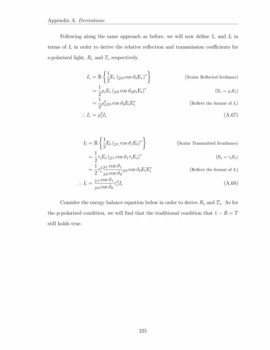
Appendix A. Derivations
Following along the same approach as before, we will now define Ir and It in
terms of Ii in order to derive the relative reflection and transmission coefficients for
s-polarized light, Rs and Ts respectively.
Ir = R
1
2Er (Y0 cosϑ0Er)
∗
(Scalar Reflected Irrdiance)
=1
2ρsEi (Y0 cosϑ0ρsEi)
∗ (Er = ρsEi)
=1
2ρ2sY0 cosϑ0EiE
∗i (Reflect the format of Ii)
∴ Ir = ρ2sIi (A.67)
It = R
1
2Et (Y1 cosϑ1Et)
∗
(Scalar Transmitted Irradiance)
=1
2τsEi (Y1 cosϑ1τsEi)
∗ (Et = τsEi)
=1
2τ 2sY1 cosϑ1
Y0 cosϑ0Y0 cosϑ0EiE
∗i (Reflect the format of Ii)
∴ It =Y1 cosϑ1
Y0 cosϑ0
τ 2s Ii (A.68)
Consider the energy balance equation below in order to derive Rs and Ts. As for
the p-polarized condition, we will find that the traditional condition that 1−R = T
still holds true.
225

Appendix A. Derivations
I0 = I1 (Conservation of energy)
R
1
2E0 ×H∗
0
= R
1
2E1 ×H∗
1
(Sub in. Eq. A.28)
R
1
2(Ei + Er) (Hi − Hr)
∗
= R
1
2EtH
∗t
(Scalar components)
1
2(Ei + Er) (Y0 cosϑ0Ei − Y0 cosϑ0Er)
∗ =1
2EtY1 cosϑ1E∗t (H = Y cosϑE)
1
2Y0 cosϑ0 (Ei + ρsEi) (Ei − ρsEi)
∗ =1
2Y1 cosϑ1τ
2sEiE
∗i (Er = ρsEi)
1
2Y0 cosϑ0EiE
∗i
(1− ρ2
s
)=
1
2Y1 cosϑ1τ
2sEiE
∗i (Factor)
=1
2Y1 cosϑ1
Y0 cosϑ0Y0 cosϑ0τ
2sEiE
∗i
Ii(1− ρ2
s
)=
1
2Y1 cosϑ1
Y0 cosϑ0
Ii (Sub. in Eq. A.66)
Ii − ρ2sIi =
1
2Y1 cosϑ1
Y0 cosϑ0
Ii (Distribute)
Ii − Ir = It (Sub in Eq. A.67, A.68)
1− IrIi
=ItIi
(Divide by Ii)
∴ 1−R = T (A.69)
Again, we will express Rs and Ts in terms of Y and ϑ.
Rs =IrIi
(Definition of Rs)
=ρ2sIiIi
(Sub in Eq. A.67)
= ρ2s (Simplify)
∴ Rs =
(Y0 cosϑ0 − Y1 cosϑ1
Y0 cosϑ0 + Y1 cosϑ1
)2
(A.70)
226

Appendix A. Derivations
Ts =ItIi
(Definition of Ts)
=τ 2s
Y1 cosϑ1
Y0 cosϑ0Ii
Ii(Sub in Eq. A.68)
= τ 2sY1 cosϑ1
Y0 cosϑ0
(Simplify)
=Y1 cosϑ1
Y0 cosϑ0
4Y20 cos2 ϑ0
(Y0 cosϑ0 + Y1 cosϑ1)2 (Sub in Eq. A.65)
∴ Ts =4Y0Y1 cosϑ0 cosϑ1
(Y0 cosϑ0 + Y1 cosϑ1)2 (A.71)
A.2.2.3 Optical admittance for oblique incidence
The optical admittance for light incident upon a surface at an oblique angle takes a
slightly different form than it did for normal incidence. Since the expressions for H
and E differ based on the polarization state of the beam, we must redefine the optical
admittance term in such a way that it applies for any obliquely incident beam upon
a non-absorbing medium, independent of its polarization. In order to distinguish this
term from the optical admittance for normal incidence, we will define it as follows:
normal incidence : η = Y = nY
oblique incidence : η =H
E
Proceeding from this definition for oblique incidence, we can derive new expres-
sions for ρ and τ that are applicable regardless of the polarization state of the incident
beam. In order to demonstrate this, we will derive the expression in sequence for p-
and s- polarizations.
227

Appendix A. Derivations
ηp =Y
cosϑ(HE for p-polarized light)
ρp =Y0
cosϑ0− Y1
cosϑ1Y0
cosϑ0+ Y1
cosϑ1
(Definition of ρp)
=ηp,0 − ηp,1ηp,0 + ηp,1
(Substitute in ηp)
(A.72)
ηs = Y cosϑ (HE for s-polarized light)
ρs =Y0 cosϑ0 − Y1 cosϑ1
Y0 cosϑ0 + Y1 cosϑ1
(Definition of ρs)
=ηs,0 − ηs,1ηs,0 + ηs,1
(Substitute in ηs)
The two derivations reveal that the amplitude reflection coefficient, ρ, can be
represented in the same manner irrespective of the polarization state of light by
writing it in terms of the optical admittance, η.
∴ ρ =η0 − η1
η0 + η1
(A.73)
Continuing in a similar manner, we can derive an expression for the ampli-
tude transmission coefficient, τ . The resultant equation is again independent of the
polarization state, provided the appropriate optical admittance is used.
ηp =Y
cosϑ(HE for p-polarized light)
τp =
2Y0
cosϑ0Y0
cosϑ0+ Y1
cosϑ1
(Definition of τp)
=2ηp,0
ηp,0 + ηp,1(Substitute in ηp)
228

Appendix A. Derivations
ηs = Y cosϑ (HE for s-polarized light)
τs =2Y0 cosϑ0
Y0 cosϑ0 + Y1 cosϑ1
(Definition of τs)
=2ηs,0
ηs,0 + ηs,1(Substitute in ηs)
∴ τ =2η0
η0 + η1
(A.74)
Based on these new definitions, we can further express the relative reflection and
transmission coefficients, R and T in terms of the optical admittance, η, as shown
below.
R =
(η0 − η1
η0 + η1
)2
(A.75)
T =4η0η1
(η0 + η1)2 (A.76)
A.2.2.4 The Brewster Angle
The equations derived above can be used to determine the degree of reflectance for
each polarization at a simple boundary between extended media. In cases wherein
there is no absorption in the medium, it can be determined that there is a definitive
angle at which the reflectance for p-polarized light goes to zero. This angle is referred
to as the Brewster Angle, but is also known as the polarizing angle, since the all of
the reflected light will be s-polarized. The expression for this angle can be derived
using a combination of Snell’s Law (Eq. A.39) and the expression for the relative
reflection coefficient for p-polarized light (Eq. A.60). Since the Brewster angle is
defined as the angle at which Rp = 0, we will start with the conditions necessary for
that outcome to occur, and derive an expression that allows us to eliminate ϑ1 from
229

Appendix A. Derivations
the expressions.
Y0
cosϑ0
=Y1
cosϑ1
(Rp = 0)
n0Ycosϑ0
=n1Y
cosϑ1
(Substitute Y = nY)
cosϑ1 =n1 cosϑ0
n0
(A.77)
n0 sinϑ0 = n1 sinϑ1 (Snell’s Law)
sinϑ1 =n0 sinϑ0
n1
(A.78)
Now that we have two independent equations, we can eliminate ϑ1 using trigono-
metric identities, as follows:
sin2 ϑ0 + cos2 ϑ0 = 1 (Trig. identity)
= sin2 ϑ1 + cos2 ϑ1 (Apply to ϑ1)
=
(n0 sinϑ0
n1
)2
+
(n1 cosϑ0
n0
)2
(Sub in Eq. A.77 and A.78)
sin2 ϑ0 −n2
0
n21
sin2 ϑ0 =n2
1
n20
cos2 ϑ0 − cos2 ϑ0 (Rearrange)(n2
1 − n20
n21
)sin2 ϑ0 =
(n2
1 − n20
n20
)cos2 ϑ0 (Isolate sin and cos)
sin2 ϑ0
cos2 ϑ0
=(n2
1 − n20)n2
1
n20 (n2
1 − n20)
(Rearrange)(sinϑ0
cosϑ0
)2
=
(n1
n0
)2
(Simplify)
tanϑ0 =n1
n0
(Trig identity)
ϑ0 = tan−1
(n1
n0
)(Solve for ϑ0)
∴ ϑB = tan−1
(n1
n0
)(A.79)
230

Appendix B
MATLAB Simulations
As a result of fabricating the original proof-of-concept waveguides in-house, certain
approximations were made due to limited resources and time constraints that neces-
sitated deviations away from our ideal designs. One such alteration was the use of the
Thorlabs LJ1878L2-A cylindrical lens adhered to the surface of a glass slab substrate,
as opposed to the use of a single piece of glass that incorporated a quarter-cylinder.
As a result, the entrance aperture of the waveguide needed to be widened slightly to
allow a sufficient amount of light to couple into the waveguide at the broader angles,
where fluence was anticipated to be greatest. The MATLAB simulations were per-
formed to determine the optimum thickness for this allowance, which was eventually
determined to be 1.0 mm wider than the radius of the lens. Waveguides were fabri-
cated with 6.0 mm entrance apertures as a result of the simulation curves generated
by the code included in this appendix.
The code incorporates a variety of necessary aspects that contribute to the
coupling efficiency of the cylindrical lens. One such aspect was the fact that as
the incident angle changed from 0 to 75°, the beam spot size would grow along its
narrowest dimension. The beam was assumed to be an elliptical gaussian, and was
simulated using a 3-dimensional intensity distribution, which was projected onto a
the waveguide surface at incident angles in 0.2° increments throughout the full range
of anticipated incident angles.
231

Appendix B. MATLAB
Another such consideration was that portions of the light would not be coupled
into the waveguide, but would instead simply reflect off the silvered rear surface of
the glass. Additionally, at broader angles, portions of the projected ellipse would
not be coupled into the waveguide as they would be incident beyond the entrance
aperture and would consequently reflect of the near face of the waveguide. The code
incorporates loops to simulate entrance apertures from 5.0 to 9.0 mm in increments
of 0.5 mm, depicting coupling efficiency resultant from the use of the cylindrical lens.
The optimum entrance aperture was chosen as the first curve that demonstrated a
maximum at 45° incidence.
kappa = .96; % Coupling efficiency
I_0 = 1.5; % Measured incident energy (mJ)
r_1 = .75; % Short axis radius (mm)
r_2 = 5; % Long axis radius (mm)
internal_angle = 1:15:75; % vary internal reflection angle
height = 1; % thickness of waveguide
var_aperture = .5;
R1 = r_1./cosd(internal_angle); % Project ellipse at an angle
R2 = r_2; % Projection does not affect R2
sigma_x = .5*R1; % Std.dev. in x
sigma_y = .5*R2; % Std.dev. in y
sigma_x_incident = .5* r_1;
A_incident = kappa .*(I_0)./(2.* pi.* sigma_x_incident .* sigma_y);
% ========================================
% Establish elliptical gaussian
[X,Y] = meshgrid ( -5:.01:5 , -10:.05:10);
Z_incident = A_incident .*exp(-(X.^2./( sigma_x_incident .^2)+Y.^2./(
sigma_y .^2)));
A_Z = sum(sum(Z_incident)); % energy of original incident beam
profile
% =====================================================
% Transmission at Reflection Interfaces
% =====================================
n_0 = 1.519; % Refractive index of waveguide
232

Appendix B. MATLAB
n_1 = 1.33; % Refractive index of tissue phantom
script_Y = 2.6544E-3; % Free space optical admittance
script_y_0 = script_Y * n_0; % Waveguide optical admittance
script_y_1 = script_Y * n_1; % Coupling oil optical admittance
theta_c = 180/pi*asin(n_1/n_0);
theta_0 = internal_angle;
L1 = 20; % active area begins 20mm from the end
L2 = 40; % active area is 20mm long
x_0 = 5; % coordinates of the center of rotation
y_0 = height;
L1_rel = L1 - x_0; % position of the active area relative to x_0
L2_rel = L2 - x_0;
Length = 60; % waveguide is 60mm long
Total_Transmission = zeros(size(internal_angle));
[aa,bb] = size(X);
for kk = 1: length(internal_angle)
% Determine reflection and transmission coefficients as a
function of
% internal reflection angle
if theta_0(kk) < theta_c
theta_1 = asind(n_0*sind(internal_angle(kk))/n_1);
T = (4* script_y_0*script_y_1*cosd(theta_0(kk))*cosd(theta_1)
) / (script_y_0*cosd(theta_0(kk)) + script_y_1*cosd(
theta_1))^2;
R = ( (script_y_0*cosd(theta_0(kk)) - script_y_1*cosd(
theta_1)) / (script_y_0*cosd(theta_0(kk)) + script_y_1*
cosd(theta_1)) )^2;
elseif theta_0(kk) == theta_c
theta_1 = 90;
T = 0;
R = 1;
else
theta_1 = theta_0(kk) + 90;
T = 0;
R = 1;
end
% =====================================================
% Internal Reflection Points
233

Appendix B. MATLAB
% ====================================
Gamma = height .*tand(internal_angle(kk)); % distance moved in
the x direction between reflection points
reflections = round(Length /( height .*tand(internal_angle(kk))));
% number of internal reflections
Transmission = zeros(length(internal_angle),reflections); %
Transmission matrix by reflection point
transmitted_Z = zeros(size(Z_incident));
reflected_Z = Z_incident;
h = waitbar(0,'Calculating reflections ...');for nn = 1: reflections
X_new = X + (2*nn -1)*Gamma;
for ii = 1:aa
for jj = 1:bb
if (L1_rel) < X_new(ii ,jj) && X_new(ii ,jj) < (L2_rel
)
% if the spot is within the active area , then
the portion
% of reflected_Z in the active area is
transmitted
transmitted_Z(ii,jj) = reflected_Z(ii,jj)*T;
reflected_Z(ii,jj) = reflected_Z(ii,jj)*R;
end
end
end
waitbar(nn/reflections ,h)
Transmission(kk ,nn) = sum(sum(transmitted_Z));
end
Total_Transmission(kk) = sum(Transmission(kk ,:));
end
plot(internal_angle ,Total_Transmission)
234

Appendix C
Error Analysis of Labview-acquired data
In recording the transmission of laser light through samples of tissue, whether for
ultrasonic modulation experiments or otherwise for waveguide active area transmis-
sion testing, substantial error was present in the data recorded by LabVIEW. Prior
to error analysis, it was not uncommon for the 90% confidence intervals of any one
test to overlap the means of other tests. These overlaps effectively invalidated many
conclusions that might have been drawn from the data, which gave rise to the need
for appropriate analysis.
This section details the error analysis and compensation process, which nar-
rowed the margin of error for each data set by iteratively accounting for each source
of non-random error and thereby reduced the standard deviations of each test indi-
vidually allowing for the drawing of meaningful inferences. The error analysis was
performed in Matlab, rather than in LabVIEW, and the code is included at the end
of this section.
235

Appendix F. Error Analysis
C.1 Identifying sources of error
The first step in compensating for error is to identify as many independent
sources as possible and subsequently categorize them as either random or systematic
errors. Random error is herein considered to be the result of unpredictable fluctua-
tions in the measurement equipment, which can be influenced by the quality of the
equipment, the accuracy of electronic components, their behavior at different tem-
peratures and energies, and other such physical influences that collectively culminate
in the generation of “white noise” in the recorded data. By contrast, systematic error
is herein considered to be the result of specific changes in the state of the measure-
ment equipment over time, which may be gradual over time or vary from one data
point to the next. For example, during the experiments conducted for Section 4,
variations in output laser energy from one shot to the next directly resulted in the
recording of peaks and valleys by both the laser energy meter and the integrating
sphere photodiode at corresponding data points (i.e. distinct spikes were observed by
both measurement devices at corresponding data points with identical indices).
The categorization of error in this manner dictates the method by which the
analysis may proceed. The principal distinguishing factor between the two varieties
of error is that random error may be averaged to yield a relatively reliable mean with
standard deviation predominantly dependent upon the quality of the measurement
equipment; whereas statistical analysis of data that is subject to systematic error
will yield means that are skewed in the direction of the error source and standard
deviations that are almost invariably greater than expected. Given that the random
236

Appendix F. Error Analysis
error is directly associated with the limitations of the equipment, which are considered
to be predominantly dependent on available grant funding, the procedural analysis of
systematic error is therefore aimed at removing the non-random deviations such that
only the random measurement error remains.
With regard to the waveguide transmission and ultrasonic modulation testing
sequences, two hundred pulses were recorded for each test, and two independent
measurements were recorded for each pulse. It was strongly suspected that the laser
energy was varying significantly from one pulse to the next, which would result in a
systematic error that would also be present in both measurements. As such, the error
at any given point can reasonably be described for the Laser Energy measurement,
L(x), and the Photocurrent, P (x) as:
L(x) = Lmean ± ErrL−measurement(x)± Errpulse(x) (C.1)
P (x) = Pmean ± ErrP−measurement(x)± Errpulse(x) (C.2)
wherein each point is defined as a deviation from the respective mean based on the
errors that are present. In this representation, ErrL−measurement and ErrP−measurement
represent the random measurement error in each measurement device, which are
considered distinct from one another. The error in incident pulse energy, Errpulse,
is present in both data sets and is considered to be resultant from the same source
of error. Accordingly it is possible to utilize one data set to remove that specific
error from the main data set of interest. It should be noted that doing so will also
necessarily merge the random error of both data sets; however, for the purposes
237

Appendix F. Error Analysis
of these experiments this is considered to be an acceptable concession, because the
random error to be removed was an order of magnitude smaller than the combined
systematic error.
NLE(x) =
(L(x)− µL
sL
)(C.3)
NP (x) =
(P (x)− µP
sP
)(C.4)
In order to confirm this assertion, the two data sets were normalized according
to Equations C.3 and C.4, where µ is the mean of the respective test sequence (not
the entire data set) and s is the corresponding standard deviation. The normalization
function converts the data into a series of points deviating around a mean of zero. If
the deviation were entirely random, there would be no observable pattern between the
two normalized data sets; however, if the deviation is not entirely random, but instead
incorporates a common systematic error, then there would be a strong correlation
between the two normalized data sets. Relatively quick options for assessing the
presence of systematic error include the Matlab command r = corr(X,Y), which
can be used to determine the correlation between two data sets X and Y, to simply
overlay the two data sets to visually observe the correlation in the data, or otherwise
to subtract one normalized data set from the other and determine if the resulting
data is normally distributed around a mean of zero with a smaller standard deviation
than either of the data presented individually. For example, figure C.1 displays the
normalized photocurrent overlaid on the normalized laser energy from a control test
sequence for the ultrasound modulation experiments. The figure clearly depicts the
238

Appendix F. Error Analysis
0 20 40 60 80 100 120 140 160 180−3
−2
−1
0
1
2
3
4
5
Repetition
NP overlaid on NL from a control test sequence
NL
NP
1
Figure C.1 Overlaying the normalized photocurrent on top of the normalizedlaser energy measurements reveals strong correlation between the errors of eachmeasurement, which confirms the influence of pulse energy variation on the mea-sured photocurrent.
strong correlation between the error shared by both data sets, with spikes and valleys
occurring in NP corresponding with spikes and valleys in NL at the same indices.
For further confirmation, this data resulted in a correlation coefficient of r = 0.9700,
which indicates strong correlation between the two and confirms the presence of the
suspected systematic error.
However, subtracting the normalized data sets may also reveal other sources
of error. For example, Figure C.1 depicts the difference of the two data sets, which
reveals that the baseline of one data set appears to “wander” and highlights outliers
that have greater than expected deviation from the mean. The analysis in this case
revealed that every 12th data point (±1) of the photocurrent yielded a greater value
239
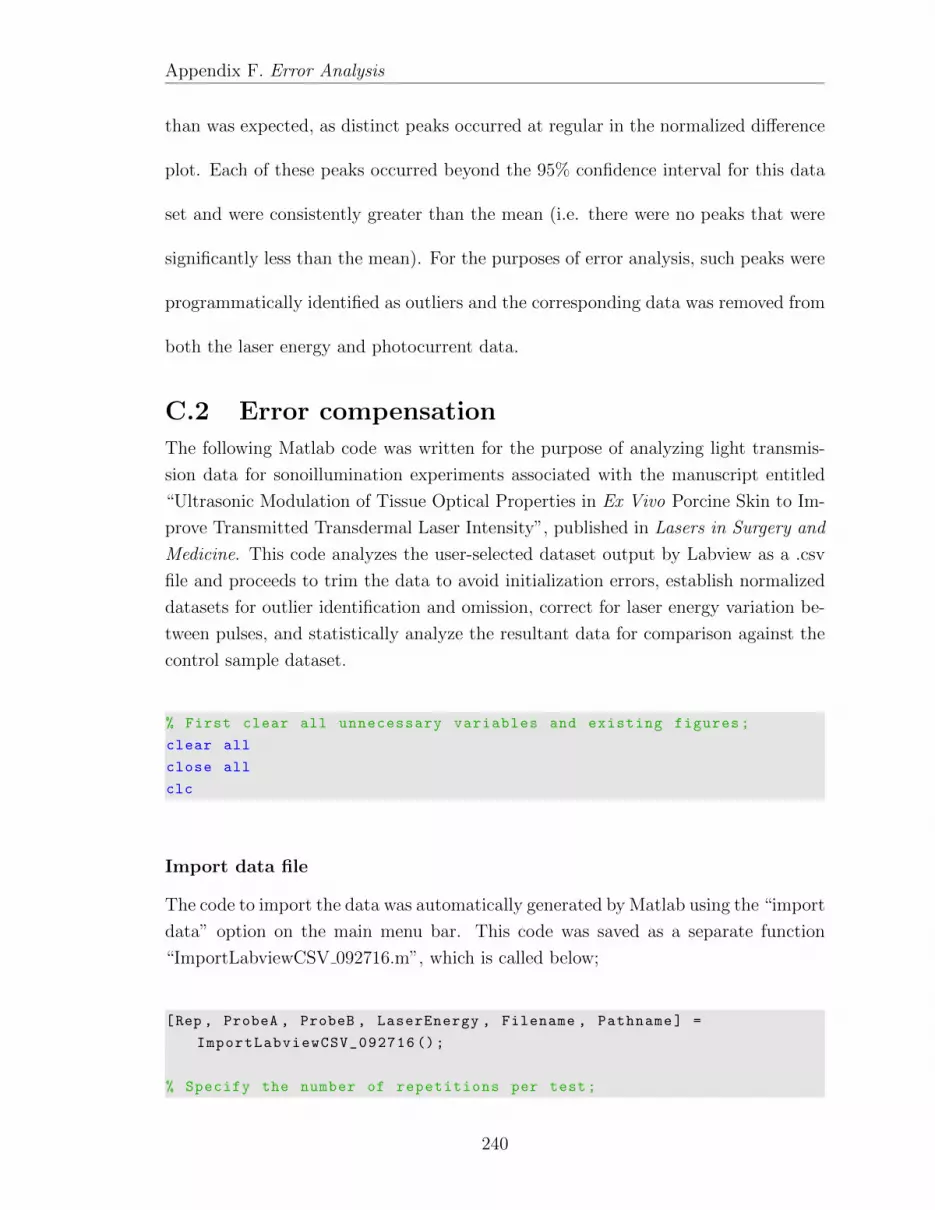
Appendix F. Error Analysis
than was expected, as distinct peaks occurred at regular in the normalized difference
plot. Each of these peaks occurred beyond the 95% confidence interval for this data
set and were consistently greater than the mean (i.e. there were no peaks that were
significantly less than the mean). For the purposes of error analysis, such peaks were
programmatically identified as outliers and the corresponding data was removed from
both the laser energy and photocurrent data.
C.2 Error compensation
The following Matlab code was written for the purpose of analyzing light transmis-
sion data for sonoillumination experiments associated with the manuscript entitled
“Ultrasonic Modulation of Tissue Optical Properties in Ex Vivo Porcine Skin to Im-
prove Transmitted Transdermal Laser Intensity”, published in Lasers in Surgery and
Medicine. This code analyzes the user-selected dataset output by Labview as a .csv
file and proceeds to trim the data to avoid initialization errors, establish normalized
datasets for outlier identification and omission, correct for laser energy variation be-
tween pulses, and statistically analyze the resultant data for comparison against the
control sample dataset.
% First clear all unnecessary variables and existing figures;
clear all
close all
clc
Import data file
The code to import the data was automatically generated by Matlab using the “import
data” option on the main menu bar. This code was saved as a separate function
“ImportLabviewCSV 092716.m”, which is called below;
[Rep , ProbeA , ProbeB , LaserEnergy , Filename , Pathname] =
ImportLabviewCSV_092716 ();
% Specify the number of repetitions per test;
240

Appendix F. Error Analysis
Num_reps = 200;
Num_tests = floor(length(Rep)./ Num_reps);
Trim the data
Omit 5 data points from the start and the end of each group to avoid skewing the
analysis via contamination from potentially saturated detectors, initial laser energy
spikes, etc.;
Num_2_remove = 5;
PA = zeros(length(Rep) -2* Num_2_remove*Num_tests ,1);
LE = PA;
r = 0;
for ii = 1: Num_tests
for jj = Num_reps *(ii -1)+ Num_2_remove + 1 : Num_reps*ii -
Num_2_remove
r = r+1;
PA(r) = ProbeA(jj);
LE(r) = LaserEnergy(jj+1);
end
end
clearvars Pathname Filename Rep ProbeA ProbeB Rep LaserEnergy ii jj
r
Predefine variables
Predefine variables to avoid memory allocation issues in subsequent loops;
Num_reps = Num_reps -2* Num_2_remove;
Mean_PA = zeros(Num_tests ,1);
Mean_LE = Mean_PA;
STD_PA = Mean_PA;
STD_LE = Mean_PA;
N_PA = zeros(size(PA));
N_LE = zeros(size(LE));
Determine means and standard deviations and build normalized datasets
241

Appendix F. Error Analysis
for ii = 1: Num_tests
Mean_PA(ii) = mean(PA(Num_reps *(ii -1) +1: Num_reps*ii));
Mean_LE(ii) = mean(LE(Num_reps *(ii -1) +1: Num_reps*ii));
STD_PA(ii) = std(PA(Num_reps *(ii -1) +1: Num_reps*ii));
STD_LE(ii) = std(LE(Num_reps *(ii -1) +1: Num_reps*ii));
for jj = Num_reps *(ii -1)+1: Num_reps*ii
N_PA(jj) = (PA(jj) - Mean_PA(ii))./ STD_PA(ii);
N_LE(jj) = (LE(jj) - Mean_LE(ii))./ STD_LE(ii);
end
end
Build N DIFF dataset
Establish a dataset that represents the non-random error (N DIFF), and calculate
the respective means and standard deviations. N DIFF is used in determining the
indices of outliers.
N_DIFF = N_PA - N_LE;
Mean_NDIFF = zeros(size(Mean_PA));
STD_NDIFF = Mean_NDIFF;
for ii = 1: Num_tests
Mean_NDIFF(ii) = mean(N_DIFF(Num_reps *(ii -1)+1: Num_reps*ii));
STD_NDIFF(ii) = std(N_DIFF(Num_reps *(ii -1)+1: Num_reps*ii));
end
Identify outliers indices
Utilize N DIFF to identify data points that occur outside the 90% Confidence Interval
for each group of 190 data points. This was typically fewer than 15 data points, which
were later identified as a non-random interference from nearby electronics;
Outlier_Indices = ones(Num_reps ,Num_tests);
PA_corrected = zeros(size(Outlier_Indices));
LE_corrected = zeros(size(Outlier_Indices));
for ii = 1: Num_tests
zz=1;
for jj = Num_reps *(ii -1)+1: Num_reps*ii
if (N_DIFF(jj) > Mean_NDIFF(ii) + STD_NDIFF(ii)*1.645 || ...
242

Appendix F. Error Analysis
N_DIFF(jj) < Mean_NDIFF(ii) - STD_NDIFF(ii)*1.645)
Outlier_Indices(zz,ii) = 0;
else
end
PA_corrected(zz ,ii) = PA(jj);
LE_corrected(zz ,ii) = LE(jj);
zz = zz+1;
end
end
PA_corrected = PA_corrected .* Outlier_Indices;
LE_corrected = LE_corrected .* Outlier_Indices;
clearvars PA LE Mean_PA Mean_LE STD_PA STD_LE Num_2_remove ii jj zz
Remove outliers and calculate statistical coefficients
Establish cell arrays containing individual data sets. Cell arrays are used because
outlier removal may result in matrices of different lengths. Calculate means and
standard deviations of the corrected data;
Mean_PA_corrected = zeros(Num_tests ,1);
Mean_LE_corrected = zeros(Num_tests ,1);
STD_PA_corrected = zeros(Num_tests ,1);
STD_LE_corrected = zeros(Num_tests ,1);
LE_finalNum_tests ,1 = [];
PA_finalNum_tests ,1 = [];
for ii = 1: Num_tests
LE_final(ii) = nonzeros(LE_corrected (:,ii));
PA_final(ii) = nonzeros(PA_corrected (:,ii));
Mean_PA_corrected(ii) = mean(cell2mat(PA_final(ii)));
STD_PA_corrected(ii) = std(cell2mat(PA_final(ii)));
Mean_LE_corrected(ii) = mean(cell2mat(LE_final(ii)));
STD_LE_corrected(ii) = std(cell2mat(LE_final(ii)));
end
Revise normalized datasets
Clear previous normalized datasets and re-establish them having omitted the outliers
243

Appendix F. Error Analysis
identified above. Calculate relevant means and standard deviations;
clearvars N_PA N_LE N_DIFF PA_corrected LE_corrected OutlierIndices;
N_PANum_tests ,1 = [];
N_LENum_tests ,1 = [];
N_DIFFNum_tests ,1 = [];
for ii = 1: Num_tests
A = cell2mat(PA_final(ii));
B = zeros(size(A));
C = cell2mat(LE_final(ii));
D = B;
for jj = 1: length(A)
B(jj) = (A(jj) - Mean_PA_corrected(ii))./ STD_PA_corrected(ii
);
C(jj) = (C(jj) - Mean_LE_corrected(ii))./ STD_LE_corrected(ii
);
end
N_PA(ii) = B;
N_LE(ii) = C;
N_DIFF(ii) = cell2mat(N_PA(ii)) - cell2mat(N_LE(ii));
end
clearvars A B C D;
Wandering baseline correction
Analysis of the data revealed that the baseline recorded by the data acquisition device
(Picoscope) was not consistent, but appeared to have a trend that varied with time.
This problem did not occur for the laser energy, however. Establish an 11-point
wandering baseline from the normalized dataset (common procedure for medical ECG
devices), subtract the moving average from the normalized dataset, and then revert
back to the original probe voltage data;
n = 11;
A = vertcat(cell2mat(N_DIFF (:)));
movingAverage = conv(A, ones(n,1)/n, 'same');
M = vertcat(cell2mat(N_PA (:))) - movingAverage;
r = 0;
244

Appendix F. Error Analysis
PA_MVavgNum_tests ,1 = [];
Mean_PA_MVavg = zeros(Num_tests ,1);
STD_PA_MVavg = Mean_PA_MVavg;
for ii = 1: Num_tests
ll = length(cell2mat(LE_final(ii)));
Mv = zeros(ll ,1);
for jj = 1:ll
r = r+1;
Mv(jj) = M(r)*STD_PA_corrected(ii) + Mean_PA_corrected(ii);
end
PA_MVavg(ii) = Mv;
Mean_PA_MVavg(ii) = mean(Mv);
STD_PA_MVavg(ii) = std(Mv);
end
clearvars n A M r ll Mean_PA_MVavg Mv movingAverage
NOTE: Analysis thus far
At this point, PA final represents the original data from ProbeA, shortened at the
ends, corrected for outliers, and corrected for the wandering baseline. The laser en-
ergy variation has yet to be taken into account. Do so by converting probe voltage
into optical power and subtracting the difference, which will yield the optical power
recorded, corrected for energy variations, with only the white noise of the measure-
ment devices as sources of error.
PA_penultimateNum_tests ,1 = [];
Mean_PA_penultimate = zeros(Num_tests ,1);
STD_PA_penultimate = Mean_PA_penultimate;
for ii = 1: Num_tests
A = cell2mat(N_LE(ii))*STD_PA_MVavg(ii);
B = cell2mat(PA_MVavg(ii)) - A;
PA_penultimate(ii) = B;
Mean_PA_penultimate(ii) = mean(B);
STD_PA_penultimate(ii) = std(B);
clearvars A B
end
245

Appendix F. Error Analysis
Unit conversion
Convert the probe voltage to equivalent optical power using a regression equation from
the data relating laser energy to probe voltage. The log regression yielded a more
accurate fit, so utilize the log relation to convert probe voltage data into equivalent
laser energy (optical power).
y => Probe Volage
x => Laser Energy
BetaFit => two element matrix of fit coefficients
Linear fit: y = BetaFit(1)*x + BetaFit(2) Log fit: y = BetaFit(1)*ln(x) + BetaFit(2)
OP_finalNum_tests ,1 = [];
Mean_OP_final = zeros(size(Mean_PA_corrected));
STD_OP_final = zeros(size(Mean_PA_corrected));
BetaFit = [62.036762824841681; -1.042597617243455e+02];
for ii = 1: Num_tests
OP_final(ii) = (exp(( cell2mat(PA_penultimate(ii)) - BetaFit (2))
/BetaFit (1)));
Mean_OP_final(ii) = mean(cell2mat(OP_final(ii)));
STD_OP_final(ii) = std(cell2mat(OP_final(ii)));
end
PLOTS
Figure 1 => Scatter plot of all data (post processed) Figure 2 => Bar plot of %
difference from control data
OP_all = vertcat(cell2mat(OP_final (:)));
X = 1: length(OP_all);
r = 0;
G = ones(size(OP_all));
for ii = 1: Num_tests
246

Appendix F. Error Analysis
ll = length(cell2mat(OP_final(ii)));
for jj = 1:ll
r = r+1;
G(r) = G(r)*ii;
end
end
figure
myColors = [0 0.2 0.75];
gscatter(X,OP_all ,G,myColors ,'psoxhd +*','','off')ax = gca;
xlabel('Repetition Number [ a.u. ]')ylabel('Transdermal Optical Power [ uJ ]')title('Transmitted transdermal optical power under varying
ultrasonic pulsation ')legend('Control ','100 mV','200 mV','300 mV','400 mV','500 mV','600
mV' ,...'700 mV','Location ','Southeast ')
set(ax ,'TickLength ' ,[0 0.01])
set(ax ,'Box','on')
clearvars X r G ii jj ll
% Scale the converted optical power based on the control dataset; i.
e.
% OP_final matrix (1);
OP_scaledNum_tests ,1 = [];
Mean_OP_scaled = zeros(size(Mean_OP_final));
STD_OP_scaled = zeros(size(Mean_OP_final));
for ii = 1: Num_tests
OP_scaled(ii) = cell2mat(OP_final(ii))./ Mean_OP_final (1);
Mean_OP_scaled(ii) = mean(cell2mat(OP_scaled(ii)));
STD_OP_scaled(ii) = std(cell2mat(OP_scaled(ii)));
end
myC = [119 178 48]./255;
myAxesLabels = ['100 ';'200 ';'300 ';'400 ';'500 ';'600 ';'700 '];
figure
myBar = barwitherr(STD_OP_scaled (2:end),Mean_OP_scaled (2:end));
ax = gca;
h = gcf;
set(ax ,'XTickLabel ',myAxesLabels)
247

Appendix F. Error Analysis
xlabel('Ultrasonic Driving Amplitude [ mV ]')ylabel('Multiplier on Control Mean Value [ a.u. ]')title('Effect of ultrasonic amplitude on scaled optical transmission
')set(ax ,'YLim' ,[1 1.9])
set(ax ,'TickLength ' ,[0 0.125])
set(ax ,'Box','on')set(myBar ,'BaseValue ' ,1.0)colormap(h,myC)
clearvars h ax myBar myC myAxesLabels ii myColors
248

Bibliography
[1] Paul J.D. Whiteside. Photonic Ablation via Quantum Tunneling. PhD thesis,
University of Missouri, May 2015.
[2] Sean W Lanigan. Lasers in dermatology. Medicine, 32(12):21 – 23, 2004.
[3] Sajjad Rajpar and Sean Lanigan. The use of lasers for dermatological condi-
tions. Medicine, 35(8):473 – 476, 2007.
[4] Sean W. Lanigan. Lasers in dermatology. Medical Laser Application, 23(2):51
– 54, 2008.
[5] Roland Kaufmann. Lasers in dermatology - state of the art. Medical Laser
Application, 20(2):103 – 109, 2005.
[6] Markolf H. Niemz. Laser-Tissue Interactions: Fundamentals and Applications.
Springer, 2004.
[7] Martin J.C. van Gemert and A.J. Welch. Clinical use of laser-tissue interactions.
Engineering in Medicine and Biology Magazine, IEEE, 8(4):10–13, Dec 1989.
249

Bibliography
[8] Barry E. DiBernardo and Jason N. Pozner. Lasers and Non-Surgical Rejuvena-
tion. Elsevier - Saunders, 2009.
[9] Elizabeth L. Tanzi, Jason R. Lupton, and Tina S. Alster. Lasers in dermatology:
Four decades of progress. Journal of the American Academy of Dermatology,
49(1):1 – 34, 2003.
[10] Jean-Paul Ortonne, Amit G. Pandya, Harvey Lui, and Doris Hexsel. Treatment
of solar lentigines. Journal of the American Academy of Dermatology, 54(5,
Supplement 2):S262 – S271, 2006.
[11] Sonal Choudhary, Mohamed L. Elsaie, Angel Leiva, and Keyvan Nouri. Lasers
for tattoo removal: a review. Lasers in Medical Science, 25(5):619–627, 2010.
[12] Michael H. Gold. Lasers and light sources for the removal of unwanted hair.
Clinics in Dermatology, 25(5):443 – 453, 2007.
[13] Carsten M. Philipp, Dagmar Scharschmidt, and H. Peter Berlien. Laser treat-
ment of scars and keloids – how we do it. Medical Laser Application, 23(2):79
– 86, 2008.
[14] J.R. Lupton, C.M. Williams, and T.S. Alster. Nonablative laser skin resur-
facing using a 1540 nm erbium glass laser: A clinical and histologic analysis.
Dermatological Surgery, 28(9), 2002.
[15] Dong Hun Lee, Yu Sung Choi, Seong Uk Min, Mi Young Yoon, and Dae Hun
250

Bibliography
Suh. Comparison of a 585-nm pulsed dye laser and a 1064-nm nd:yag laser for
the treatment of acne scars: A randomized split-face clinical study. Journal of
the American Academy of Dermatology, 60(5):801 – 807, 2009.
[16] Lisa Carroll and Tatyana R. Humphreys. Laser-tissue interactions. Clinics in
Dermatology, 24(1):2 – 7, 2006.
[17] Maurice A. Adatto. Laser tattoo removal: Benefits and caveats. Medical Laser
Application, 19(4):175 – 185, 2004.
[18] Akkrapol Mungnirandr, Woraphong Manuskiatti, Pakawadee Hatthanirun,
Wanwilai Outtarawichian, Sakda Sookruen, Chaiwat Buathong, and Yongyuth
Vajaradul. Laser tattoo removal in thai students. Medical Laser Application,
26(3):126 – 132, 2011.
[19] Katy Burris and Karen Kim. Tattoo removal. Clinics in Dermatology, 25(4):
388 – 392, 2007.
[20] Uwe Wollina and Erich Kostler. Tattoos: surgical removal. Clinics in Derma-
tology, 25(4):393 – 397, 2007.
[21] Theodora Kossida, Dimitrios Rigopoulos, Andreas Katsambas, and R. Rox An-
derson. Optimal tattoo removal in a single laser session based on the method
of repeated exposures. Journal of the American Academy of Dermatology, 66
(2):271 – 277, 2012.
251

Bibliography
[22] Eric F. Bernstein. Laser treatment of tattoos. Clinics in Dermatology, 24(1):
43 – 55, 2006.
[23] Keyvan Nouri and Christopher J. Ballard. Laser therapy for acne. Clinics in
Dermatology, 24(1):26 – 32, 2006.
[24] H-J. Laubach, Z. Tannous, R.R. Anderson, and D. Manstein. Skin responses
to fractional photothermolysis. Lasers in Surgery and Medicine, 38, 2006.
[25] Pa-Fan Hsiao, Yang-Chih Lin, Cheng-Chieh Huang, and Yu-Hung Wu. Efficacy
and safety of a single treatment using a 10,600-nm carbon dioxide fractional
laser for mild-to-moderate atrophic acne scars in asian skin. Dermatologica
Sinica, 31(2):59 – 63, 2013.
[26] Karen Riggs, Matthew Keller, and Tatyana R. Humphreys. Ablative laser
resurfacing: high-energy pulsed carbon dioxide and erbium:yttrium-aluminum-
garnet. Clinics in Dermatology, 25(5):462 – 473, 2007.
[27] Naga B. Meduri. Facial resurfacing: An overview. Operative Techniques in
Otolaryngology-Head and Neck Surgery, 18(3):172 – 180, 2007.
[28] Macrene R. Alexiades-Armenakas, Jeffrey S. Dover, and Kenneth A. Arndt.
The spectrum of laser skin resurfacing: Nonablative, fractional, and ablative
laser resurfacing. Journal of the American Academy of Dermatology, 58(5):719
– 737, 2008.
252

Bibliography
[29] Khaled M. Hassan and Anthony V. Benedetto. Facial skin rejuvenation: Ab-
lative laser resurfacing, chemical peels, or photodynamic therapy? facts and
controversies. Clinics in Dermatology, 31(6):737 – 740, 2013.
[30] Danielle M. DeHoratius and Jeffrey S. Dover. Nonablative tissue remodeling
and photorejuvenation. Clinics in Dermatology, 25(5):474 – 479, 2007.
[31] Albert E. Rivera. Acne scarring: A review and current treatment modalities.
Journal of the American Academy of Dermatology, 59(4):659 – 676, 2008.
[32] Zeina Tannous. Fractional resurfacing. Clinics in Dermatology, 25(5):480 – 486,
2007.
[33] Jeffrey S. Orringer, Sewon Kang, Timothy M. Johnson, Darius J. Karimipour,
Ted Hamilton, Craig Hammerberg, John J. Voorhees, and Gary J. Fischer.
Connective tissue remodeling induced by carbon dioxide laser resurfacing of
photodamaged human skin. Archives of Dermatology, 140(11):1326–1332, 2004.
[34] Kenneth C. Nowak, Matthew McCormack, and R. James Koch. The effect of
superpulsed carbon dioxide laser energy on keloid and normal dermal fibroblast
secretion of growth factors: A serum-free study. Plastic and Reconstructive
Surgery, 105(6), 2000.
[35] S. Parker. Verifiable cpd paper: Laser-tissue interaction. British Dental Journal,
202:73–81, 2007.
253
Bibliography
[36] A.J. Welch. The thermal response of laser irradiated tissue. Quantum Electron-
ics, IEEE Journal of, 20(12):1471–1481, December 1984.
[37] Ashley J. Welch and Martin J.C. van Gemert, editors. Optical-Thermal
Response of Laser-Iradiated Tissue. Lasers, Photonics, and Electro-Optics.
Plenum Press, 1st edition, 1995.
[38] Darwin D.-M. Ho, Richard London, George B. Zimmerman, and David A.
Young. Laser-tattoo removal—a study of the mechanism and the optimal treat-
ment strategy via computer simulations. Lasers in Surgery and Medicine, 30
(5):389–397, 2002.
[39] Victor E. Ross, George Naseef, Charles Lin, Michael Kelly, Norm Michaud,
Thomas J. Flotte, Jill Raythen, and R. Rox Anderson. Comparison of re-
sponses of tattoos to picosecond and nanosecond q-switched neodymium:yag
lasers. Archives of Dermatology, 134(2):167–171, 1998.
[40] John C. Fisher. Photons, physiatrics, and physicians- a practical guide to under-
standing interaction of laser light with living tissue- part ii: Basic mechanisms
of tissue destruction by laser beams. Journal of Clinical Laser Medicine and
Surgery, 11(6):291–303, 1993.
[41] F. Hillenkamp. Laser radiation tissue interaction. Health Physics, 56(5):613–6,
May 1989.
[42] Stanley M. Shapshay, editor. Endoscopic Laser Surgery Handbook. Science and
254

Bibliography
Practice of Surgery. Marcel Dekker, Inc., 1987.
[43] K. Shokrollahi, E. Raymond, and M.S.C. Murison. Lasers: Principles and
surgical applications. The Journal of Surgery, 2(1), 2004.
[44] Robert S. Anderson, Robert E. Hermes, Gennady A. Matyushin, Vladimir S.
Nechitailo, and Stephen C. Picarello. Photostability of dye-doped modified
polymers at extremely high intensities: Medlite laser systems. Proceedings of
the SPIE, 3265:13–20, 1998.
[45] Cynosure medlite c6 medical laser description. 2014. URL http://www.
cynosure.com/products/medlite/howitworks.php.
[46] Solta medical fraxel laser system. 2014. URL http://www.solta.com/brands/
fraxel.
[47] L. Goldman, D.J. Blaney, D.J. Kindel, and E.K. Franke. Effect of the laser
beam on the skin. Journal of Investigative Dermatology, 40:121–122, 1963.
[48] L. Goldman, D.J. Blaney, D.J. Kindel, D. Richfield, and E.K. Franke. Pathology
of the effect of the laser beam on the skin. Nature, 197(912-914), 1963.
[49] Yaniv Barkana and Michael Belkin. Laser eye injuries. Survey of Ophthalmology,
44(6):459 – 478, 2000.
[50] Daniel F Marcus, Md, and James Ravin. A new report of laser eye injury.
Survey of Ophthalmology, 45(3), 2000.
255

Bibliography
[51] Michael Belkin. Authors’ response: A new report on laser eye injuries. Survey
of Ophthalmology, 45(3):262 – 263, 2000.
[52] Daniele De Luca, Ines Delfino, and Maria Lepore. Laser safety standards and
measurements of hazard parameters for medical lasers. International Journal
of Optics and Applications, 2(6):80–86, 2012.
[53] Benjamin A. Rockwell, Robert J. Thomas, and Alfred Vogel. Ultrashort laser
pulse retinal damage mechanisms and their impact on thresholds. Medical Laser
Application, 25(2):84 – 92, 2010.
[54] Alfred Schirmacher. Eye protection for short and ultra-short pulsed laser sys-
tems. Medical Laser Application, 25(2):93 – 98, 2010.
[55] Ming Chen, Chunfei Li, Mai Xu, Weibiao Wang, Shaojie Ma, and Yuxue Xia.
Eye-protection glasses against yag laser injury based on the band gap reflection
of one-dimensional photonic crystal. Optics and Laser Technology, 39(1):214 –
218, 2007.
[56] Moshe Lapidoth, Gal Shafirstein, Dan Ben Amitai, Emmilia Hodak, Milton
Waner, and Michael David. Reticulate erythema following diode laser-assisted
hair removal: A new side effect of a common procedure. Journal of the American
Academy of Dermatology, 51(5):774 – 777, 2004.
[57] Sean W Lanigan. Incidence of side effects after laser hair removal. Journal of
the American Academy of Dermatology, 49(5):882 – 886, 2003.
256

Bibliography
[58] Christopher A. Nanni and Tina S. Alster. Laser-assisted hair removal: Side
effects of q-switched nd:yag, long-pulsed ruby, and alexandrite lasers. Journal
of the American Academy of Dermatology, 41(2):165 – 171, 1999.
[59] Sara Friedman and Jonathan Lippitz. Chemical peels, dermabrasion, and laser
therapy. Disease-a-Month, 55(4):223 – 235, 2009.
[60] E. Z. Zhang, J. G. Laufer, R. B. Pedley, and P. C. Beard. In vivo high-resolution
3d photoacoustic imaging of superficial vascular anatomy. Physics in Medicine
and Biology, 54(4):1035–1046, 2009.
[61] James A. Guggenheim, Thomas J. Allen, Andrew Plumb, Edward Z. Zhang,
Manuel Rodriguez-Justo, Shonit Punwani, and Paul C. Beard. Photoacoustic
imaging of human lymph nodes with endogenous lipid and hemoglobin contrast.
Journal of Biomedical Optics, 20(5), 2015.
[62] E.B. Samson, B.S. Goldschmidt, P.J.D. Whiteside, A.S.M. Sudduth, J.R.
Custer, B. Beernsten, and J.A. Viator. Photoacoustic spectroscopy of beta-
hematin. Journal of Optics, 14(6), 2012.
[63] Edward Z. Zhang, Jan Laufer, and Paul Beard. Backward-mode multiwave-
length photoacoustic scanner using a planar fabry-perot polymer film ultra-
sound sensor for high-resolution three-dimensional imaging of biological tissues.
Applied Optics, 47(4):561–577, 2008.
[64] B.T. Cox and P.C. Beard. The frequency-dependent directivity of a planar
257

Bibliography
fabry-perot polymer film ultrasound sensor. Ultrasonics, Ferroelectrics, and
Frequency Control, IEEE Transactions on, 54(2):394–404, 2007.
[65] Paul Morris, Andrew Hurrell, Adam Shaw, Edward Zhang, and Paul Beard. A
fabry-perot fiber-optic ultrasonic hydrophone for the simultaneous measurement
of temperature and acoustic pressure. The Journal of the Acoustical Society of
America, 125(6):3611–3622, 2009.
[66] Paul J. D. Whiteside, Benjamin S. Goldschmidt, Randy Curry, and John A. Via-
tor. Controlled laser delivery into biological tissue via thin-film optical tunneling
and refraction. Proceedings of the SPIE, 9303, 2015. doi: 10.1117/12.2078994.
[67] Mason W. Schellenberg, Paul J.D. Whiteside, and Heather K. Hunt. Planar
waveguide light transmission modality for backward-mode photoacoustic to-
mography. Proceedings of the SPIE, 9708, 2016.
[68] Paul J.D. Whiteside, Nicholas J. Golda, Randy D. Curry, and John A. Via-
tor. Regulation of evanescent leaking for contact-based light transmission in
biophotonics applications. Applied Optics, 2017.
[69] G. Li, Y. Hashimoto, T. Maruyama, and K. Iiyama. High-efficiency optical
coupling to planar photodiode using metal reflector loaded waveguide grating
coupler. Optical and Quantum Electronics, 45(7):657–663, 2013.
[70] Milan Milosevic. Internal Reflection and ATR Spectroscopy, volume 176 of
Chemical Analysis. Wiley, 2012.
258

Bibliography
[71] Siang Ping Ng and J.I. Mackenzie. Planar waveguide laser optimization and
characterization employing real-time beam quality measurement. IEEE Journal
of Quantum Electronics, 49(2):146–153, Feb 2013.
[72] M.N. Polyanskiy. Refractive index database, 2015. URL:
http://refractiveindex.info.
[73] A.D. Rakic, A.B. Djurisic, J.M. Elazar, and M.L. Majewski. Optical properties
of metallic films for vertical cavity optoelectronic devices. Applied Optics, 37:
5271–5283, 1998.
[74] B.A. Sexton, B.N. Feltis, and T.J. Davis. Characterisation of gold surface
plasmon resonance sensor substrates. Sensors and Actuators A: Physical, 141
(2):471 – 475, 2008.
[75] J.C. Hoogvliet and W.P. van Bennekom. Gold thin-film electrodes: an EQCM
study of the influence of chromium and titanium adhesion layers on the re-
sponse. Electrochimica Acta, 47(4):599 – 611, 2001. doi: http://dx.doi.org/10.
1016/S0013-4686(01)00793-9.
[76] Paul J.D. Whiteside, Jeffrey A. Chininis, and Heather K. Hunt. Techniques and
challenges for characterizing metal thin films with applications in photonics.
Coatings, 6(3):35, 2016.
[77] Gabriel Maria Ingo, Giuseppe Guida, Emma Angelini, Gabriella Di Carlo,
Alessio Mezzi, and Giuseppina Padeletti. Ancient mercury-based plating meth-
259

Bibliography
ods: Combined use of surface analytical techniques for the study of manufac-
turing process and degradation phenomena. Accounts of Chemical Research, 46
(11):2365–2375, 2013. doi: 10.1021/ar300232e.
[78] Hosuk Lee, Hosun Lee, Jun-Hyuk Park, Han-Ki Kim, Bo Hyun Kong, and
Hyung Koun Cho. Optical properties of ultrathin copper thin films sandwiched
between nb-doped tio 2 films studied with spectroscopic ellipsometry. Japanese
Journal of Applied Physics, 50(5R):055805, 2011.
[79] H. Kuhn and B. A. Wilson. Reflectivity of thin silver films and their use in
interferometry. Proceedings of the Physical Society. Section B, 63(10):745, 1950.
[80] E.S.O. New adaptive optics component delivered for the eso vlt, 2 March,
2012. URL http://www.eso.org/public/announcements/ann12015/. URL:
http://www.eso.org/public/announcements/ann12015/.
[81] Enrico Savazzi. Digital Photography for Science: Close-Up Photography,
Macrophotography, and Photomacrography. Enrico Savazzi, 2011.
[82] Hans Jurgen Karcher. Reflecting Telescope Mechanics. Wiley VCH Cerlag
GmbH, 2008.
[83] Jeffrey Chininis, Paul J.D. Whiteside, and Heather K. Hunt. Metal-clad waveg-
uide characterization for contact-based light transmission into tissue. Proceed-
ings of the SPIE, 9689, 2016.
260

Bibliography
[84] Ding Lei, Zhang Fanghui, Ma Ying, and Zhang Maili. Aluminum/moo3 anode
thin films: an effective anode structure for high-performance flexible organic
optoelectronics. Journal of Semiconductors, 33(1), January 2012.
[85] Sihai Chen, Hong Ma, Xinjian Yi, Hongcheng Wang, Xiong Tao, Mingxiang
Chen, Xiongwei Li, and Caijun Ke. Optical switch based on vanadium dioxide
thin films. Infrared Physics & Technology, 45(4):239 – 242, 2004.
[86] M. Jlassi, I. Sta, M. Hajji, and H. Ezzaouia. Optical and electrical properties
of nickel oxide thin films synthesized by sol–gel spin coating. Materials Science
in Semiconductor Processing, 21:7 – 13, 2014. doi: http://dx.doi.org/10.1016/
j.mssp.2014.01.018.
[87] J. Hotovy, J. Hupkes, W. Bottler, E. Marins, L. Spiess, T. Kups, V. Smirnov,
I. Hotovy, and J. Kovac. Sputtered ito for application in thin-film silicon solar
cells: Relationship between structural and electrical properties. Applied Surface
Science, 269:81 – 87, 2013. doi: http://dx.doi.org/10.1016/j.apsusc.2012.10.180.
[88] M. Choobtashani and O. Akhavan. Visible light-induced photocatalytic reduc-
tion of graphene oxide by tungsten oxide thin films. Applied Surface Science,
276:628 – 634, 2013. doi: http://dx.doi.org/10.1016/j.apsusc.2013.03.144.
[89] K.J. Kuhn. Laser Engineering. Prentice-Hall, 1998.
[90] E. Hecht. Optics. Addison Wesley, 4th edition edition, 2001.
261

Bibliography
[91] Max Born and Emil Wolf. Principles of Optics: Electromagnetic theory of
propagation, interference and diffraction of light. Cambridge University Press,
seventh edition edition, 1999.
[92] Katsunari Okamoto. Fundamentals of Optical Waveguides. Elsevier Academic
Press, 2nd edition edition, 2006.
[93] N. J. Harrick. Internal Reflection Spectroscopy. Harrick Scientific Corporation,
3rd edition edition, 1987.
[94] L. Novotny and B. Hecht. Principles of Nano-Optics. Cambridge University
Press, 2nd edition, 2012.
[95] S. Zhu, A. W. Yu, D. Hawley, and R. Roy. Frustrated total internal reflection:
A demonstration and review. American Journal of Physics, 54(7):601–607, July
1986.
[96] J. Domaradzki, S. Lis, D. Kaczmarek, and S. Patela. Application of spec-
trophotometry and ellipsometry for determination of optical parameters of op-
tical coating thin films. Students and Young Scientists Workshop, 2010 IEEE
International, pages 10–13, 2010.
[97] M. Kusko, M. Purica, and E. Budianu. The optical characterization of thin
layers by spectrophotometry measurements. International Semiconductor Con-
ference, 1:90 Vol. 1, 2003.
262

Bibliography
[98] Yang Gan. Atomic and subnanometer resolution in ambient conditions by
atomic force microscopy. Surface Science Reports, 64(3):99 – 121, 2009. doi:
http://dx.doi.org/10.1016/j.surfrep.2008.12.001.
[99] Dimitrios Fotiadis, Simon Scheuring, Shirley A. Muller, Andreas Engel, and
Daniel J. Muller. Imaging and manipulation of biological structures with
the AFM. Micron, 33(4):385 – 397, 2002. doi: http://dx.doi.org/10.1016/
S0968-4328(01)00026-9.
[100] R. Escobar Galindo, R. Gago, A. Lousa, and J.M. Albella. Comparative depth-
profiling analysis of nanometer-metal multilayers by ion-probing techniques.
TrAC Trends in Analytical Chemistry, 28(4):494–505, 2009.
[101] A. Torres Perez, A. Hernandez Battez, G. Garcıa-Atance, J.L. Viesca,
R. Gonzalez, and M. Hadfield. Use of optical profilometry in the ASTM
D4172 standard. Wear, 271(11–12):2963 – 2967, 2011. doi: http://dx.doi.
org/10.1016/j.wear.2011.06.016.
[102] S. Sharp, S. Burgess, C. Hodson, and Q. Fang. Thin film properties measure-
ment using sem-based energy dispersive spectroscopy for nanoscience studies.
Microscopy and Microanalysis, 14:336–337, 2008.
[103] K.D. Vernon-Parry. Scanning electron microscopy: an introduction. III-Vs
Review, 13(4):40 – 44, 2000. doi: http://dx.doi.org/10.1016/S0961-1290(00)
80006-X.
263

Bibliography
[104] Jean-Louis Pouchou. X-ray microanalysis of stratified specimens. Analyt-
ica Chimica Acta, 283(1):81 – 97, 1993. doi: http://dx.doi.org/10.1016/
0003-2670(93)85212-3.
[105] M. Procop, M. Radtke, M. Krumrey, K. Hasche, S. Schadlich, and W. Frank.
Electron probe microanalysis (epma) measurement of thin-film thickness in the
nanometer range electron probe microanalysis (epma) measurement of thin-film
thickness in the nanometer range. Analytical and Bioanalytical Chemistry, 374
(631-634), 2002.
[106] Benjamin S. Goldschmidt, Anna M. Rudy, Charissa A. Nowak, Dylan P. Ma-
coubrie, John A. Viator, and Heather K. Hunt. Characterization of mgf2 thin
films using optical tunneling photoacoustic spectroscopy. Optics & Laser Tech-
nology, 73:146–155, 2015.
[107] Jorge Pisonero, Beatriz Fernandez, Rosario Pereiro, Nerea Bordel, and Alfredo
Sanz-Medel. Glow-discharge spectrometry for direct analysis of thin and ultra-
thin solid films. TrAC Trends in Analytical Chemistry, 25(1):11 – 18, 2006. doi:
http://dx.doi.org/10.1016/j.trac.2005.04.019.
[108] Marcus Wilke, Gerd Teichert, Ryota Gemma, Astrid Pundt, Reiner Kirch-
heim, Henry Romanus, and Peter Schaaf. Glow discharge optical emission
spectroscopy for accurate and well resolved analysis of coatings and thin films.
Thin Solid Films, 520(5):1660 – 1667, 2011. doi: http://dx.doi.org/10.1016/j.
tsf.2011.07.058.
264

Bibliography
[109] S. Hosoi, K. Nakajima, M. Suzuki, K. Kimura, Y. Shimizu, S. Fukatsu, K.M.
Itoh, M. Uematsu, H. Kageshima, and K. Shiraishi. Observation of si emission
during thermal oxidation of si(0 0 1) with high-resolution RBS. Nuclear
Instruments and Methods in Physics Research Section B: Beam Interactions
with Materials and Atoms, 249(1–2):390 – 393, 2006. doi: http://dx.doi.org/
10.1016/j.nimb.2006.04.036.
[110] R. Nagel, C. Alof, A.G. Balogh, W.M. Arnoldbik, and D.O. Boerma. Study
of magnetic multilayers by RBS with nanometer resolution. Nuclear Instru-
ments and Methods in Physics Research Section B: Beam Interactions with
Materials and Atoms, 183:140 – 145, 2001. doi: http://dx.doi.org/10.1016/
S0168-583X(01)00320-2.
[111] P Bailey, T.C.Q Noakes, C.J Baddeley, S.P Tear, and D.P Woodruff. Monolayer
resolution in medium energy ion scattering. Nuclear Instruments and Methods
in Physics Research Section B: Beam Interactions with Materials and Atoms,
183:62 – 72, 2001. doi: http://dx.doi.org/10.1016/S0168-583X(01)00384-6.
[112] M. Branescu, C. Naudin, M. Gartner, and G. Nemes. Depth profiling raman
spectroscopy of a thin yba2cu3o7 δ film. Thin Solid Films, 516(22):8190 – 8194,
2008. doi: http://dx.doi.org/10.1016/j.tsf.2008.04.074.
[113] Yasushi Oshikane, Toshihiko Kataoka, Mitsuru Okuda, Seiji Hara, Haruyuki
Inoue, and Motohiro Nakano. Observation of nanostructure by scanning near-
field optical microscope with small sphere probe. Science and Technology of
265

Bibliography
Advanced Materials, 8(3):181, 2007.
[114] Bharat Bhushan. Surface roughness analysis and measurement techniques. In
Bharat Bhushan, editor, Modern Tribology Handbook, volume 1, chapter 2. CRC
Press, 2000.
[115] Michael C. Howland, Alan W. Szmodis, Babak Sanii, and Atul N. Parikh.
Characterization of physical properties of supported phospholipid membranes
using imaging ellipsometry at optical wavelengths. Biophysical Journal, 92(4):
1306 – 1317, 2007. doi: http://dx.doi.org/10.1529/biophysj.106.097071.
[116] K. Drogowska, Z. Tarnawski, A. Brudnik, E. Kusior, M. Soko lowski, K. Za-
krzewska, A. Reszka, N. T. H. Kim-Ngan, and A. G. Balogh. Rbs, xrr and
optical reflectivity measurements of ti–tio2 thin films deposited by magnetron
sputtering. Materials Research Bulletin, 47(2):296–301, 2012.
[117] E. Chason and T. M. Mayer. Thin film and surface characterization by specular
x-ray reflectivity. Critical Reviews in Solid State and Materials Sciences, 22(1):
1–67, 1997.
[118] Jens Als-Nielsen and Des McMorrow. Refraction and reflection from interfaces,
pages 69–112. Wiley, 2011. doi: 10.1002/9781119998365.ch3.
[119] A. Kossoy, D. Simakov, S. Olafsson, and K. Leosson. Determining surface
coverage of ultra-thin gold films from x-ray reflectivity measurements. Thin
Solid Films, 536(0):50–53, 2013.
266

Bibliography
[120] Michael F. Toney and Sean Brennan. Measurements of carbon thin films using
x-ray reflectivity. Journal of Applied Physics, 66(4):1861–1863, 1989.
[121] Robert W. Collins and Yeon Taik Kim. Ellipsometry for thin-film and surface
analysis. Analytical Chemistry, 62(17):887A–890A, 1990.
[122] R. M. A. Azzam and N. M. Bashara. Ellipsometry and polarized light. North-
Holland Pub. Co., 1977.
[123] Karsten Hinrichs, Andreas Furchner, Guoguang Sun, Michael Gensch, Jorg
Rappich, and Thomas W. H. Oates. Infrared ellipsometry for improved laterally
resolved analysis of thin films. Thin Solid Films, 571(3):648–652, 2014.
[124] I. Kalimanova, N. Ilieva, and M. Georgieva. Ellipsometry and thin films param-
eters measurement. 28th International Spring Seminar on Electronics Technol-
ogy: Meeting the Challenges of Electronics Technology Progress, pages 472–475,
2005.
[125] M. Horprathum, J. Kaewkhao, P. Eiamchai, P. Chindaudom, and P. Limsuwan.
Investigation of inhomogeneity of tio2 thin films using spectroscopic ellipsome-
try. Journal of Physics: Conference Series, 417(1), 2013.
[126] Dawn Bonnel, editor. Scanning Probe Microscopy and Spectroscopy: Theory,
Techniques, and Applications. Wiley, 2nd edition, 2000.
[127] G. Binnig, C. Quate, and Ch Gerber. Atomic force microscope. Physical Review
267

Bibliography
Letters, 56(9):930–933, 1986.
[128] R.F.M. Lobo, M.A. Pereira-da Silva, M. Raposo, R.M. Faria, and O.N.
Oliveira Jr. In situ thickness measurements of ultra-thin multilayer polymer
films by atomic force microscopy. Nanotechnology, 10:389–393, 1999.
[129] Po-Jui Su and Bernard Haochih Liu. Ion-beam-sputter deposited titanium ni-
tride thin films for conductive atomic force microscope probes. Thin Solid Films,
529(0):317–321, 2013. doi: http://dx.doi.org/10.1016/j.tsf.2012.07.066.
[130] J.I. Goldstein. Scanning Electron Microscopy and X-Ray Microanalysis.
Springer, 3rd edition, 2003.
[131] F. Z. Mammeri, L. Chekour, and N. Rouag. Characterization of nitride thin
films using sem and edx. Acta Physica Polonica, A, 123(2):294–295, 2013.
[132] Matthew T. Johnson, C. Barry Carter, and Joseph Michael. Sem analysis of
oxide thin films and reactions. Journal of the American Ceramic Society, 82
(6):1644–1646, 1999.
[133] Barbara G. Kutchko and Ann G. Kim. Fly ash characterization by sem-eds.
Fuel, 85(17-18):2537 – 2544, 2006. doi: http://dx.doi.org/10.1016/j.fuel.2006.
05.016.
[134] Michael C. Meyer, Peter Austin, and Peter Tropper. Quantitative evaluation of
mineral grains using automated sem–eds analysis and its application potential
268

Bibliography
in optically stimulated luminescence dating. Radiation Measurements, 58:1 –
11, 2013. doi: http://dx.doi.org/10.1016/j.radmeas.2013.07.004.
[135] E. D. Boyes. Nanoparticle, thin film and surface sensitive analysis in the sem.
Microscopy and Microanalysis, 13:584–585, 2007.
[136] B.S. Goldschmidt, A.S.M Sudduth, P.J.D. Whiteside, and J.A. Viator. Total
internal reflection photoacoustic spectroscopy. U.S. Patent App. 13/747,172,
2013.
[137] B. S. Goldschmidt, A. S. M. Sudduth, E. Samson, P. J. D. Whiteside, K. Bhat-
tacharyya, and J. A. Viator. Total internal reflection photoacoustic spectroscopy
for the detection of beta-hematin. Journal of Biomedical Optics, 17(6), 2012.
[138] Amanda S. M. Sudduth, Benjamin S. Goldschmidt, Edward B. Samson, Paul
J. D. Whiteside, and John A. Viator. Total internal reflection photoacoustic
detection spectroscopy. Proc. SPIE, 7899, 2011.
[139] Charles Vassallo. Optical Waveguide Concepts, volume 1 of Optical Wave Sci-
ences and Technology. Elsevier, 1991.
[140] H. Angus Macleod. Thin-Film Optical Filters. Institute of Physics, third edition
edition, 2001.
[141] Robert G. Hunsperger. Integrated Optics. Springer, 6th edition edition, 2009.
[142] Choon-Gi Choi, Sang-Pil Han, and Myung-Yung Jeong. Two-dimensional poly-
269

Bibliography
meric optical waveguides for high-density parallel optical interconnection. Op-
tics Communications, 235:69 – 73, 2004.
[143] Sir Isaac Newton. Opticks: A Treatise of the Reflections, Refractions, Inflections
and Colours of Light. London : Printed for William Innys at the West-End of
St. Paul’s, 4th edition edition, 1730.
[144] Benjamin S. Goldschmidt. Photoacoustic Evaluation of Surfaces via Pulsed
Evanescent Field Interaction. PhD thesis, University of Missouri, May 2014.
[145] I.N. Court and F.K. von Willisen. Frustrated total internal reflection and ap-
plication of its principle to laser cavity design. Applied Optics, 3(6):719–726,
June 1964.
[146] P.K. Tien and R. Ulrich. Theory of prism-film coupler and thin-film light guides.
Journal of the Optical Society of America, 60(10):1325–1337, October 1970.
[147] P.W. Baumeister. Optical tunneling and its applications to optical filters. Ap-
plied Optics, 6(5), 1967.
[148] R. Ulrich and R. Torge. Measurement of thin film parameters with a prism
coupler. Applied Optics, 12(12), 1973.
[149] Yu Zhu, Chuanjun Yao, Jinbang Chen, and Rihong Zhu. Frustrated total in-
ternal reflection evanescent switching. Optics and Laser Technology, 31(8):539
– 542, 1999.
270

Bibliography
[150] S.B. Kharchenko, P.M. McGuiggan, and K.B. Migler. Flow induced coating
of fluoropolymer additives: Development of frustrated total internal reflection
imaging. Journal of Rheology, 47(1523), 2003.
[151] Nicholas J. Goddard, Kirat Singh, Richard J. Holmes, and Behnam Bastani.
Resonant grating sensors using frustrated total-internal reflection. Sensors and
Actuators B: Chemical, 51(1–3):131 – 136, 1998.
[152] Frederique de Fornel. Evanescent Waves From Newtonian Optics to Atomic
Optics. Springer, 1st edition, 2001.
[153] K. Forsterling. Uber die messung der optischen konstanten sehr dunner met-
allschichten. Annalen der Physik, 422(8):745–751, 1937.
[154] J. Stuart Nelson, Thomas E. Milner, Bahman Anvari, B. Samuel Tanenbaum,
Sol Kimel, Lars O. Svaasand, and Steven L. Jacques. Dynamic epidermal cool-
ing during pulsed laser treatment of port-wine stain: A new methodology with
preliminary clinical evaluation. Archives of Dermatology, 131(6):695–700, 1995.
[155] Paul J.D. Whiteside, Chenxi Qian, Nicholas J. Golda, and Heather K. Hunt.
Ultrasonic modulation of tissue optical properties in ex vivo porcine skin to im-
prove transmitted transdermal laser intensity. Lasers in Surgery and Medicine,
?(?):?–?, 2017.
[156] Mona Boord. Laser in dermatology. Clinical Techniques in Small Animal Prac-
tice, 21(3):145–149, 2008.
271

Bibliography
[157] Franz-Xaver Schmid. Biological Macromolecules: UV-visible Spectrophotometry.
Encyclopedia of Life Sciences. Nature Publishing Group, 2001.
[158] Rami Nachabe, Benno H.W. Hendriks, Marjolen van der Voort, Adrien E. Des-
jardins, and Henricus J.C.M. Sterenborg. Estimation of biological chromophores
using diffuse optical spectroscopy: benefit of extending the uv-vis wavelength
range to include 1000 to 1600 nm. Biomedical Optics Express, 1(5):1432–1442,
2010.
[159] Paul Beard. Biomedical photoacoustic imaging. Interface Focus, 1(4), 2011.
[160] Scott Prahl. Tabulated molar extinction coefficient for hemoglobin
in water. Oregon Medical Laser Center, 1998. URL:
http://omlc.org/spectra/hemoglobin/index.html.
[161] Steven L. Jacques, Randolph D. Glickman, and Jon A. Schwartz. Internal
absorption coefficient and threshold for pulsed laser disruption of melanosomes
isolated from retinal pigment epithelium. Proceedings of the SPIE, 468, May
1996.
[162] A. F. Alexis. Lasers and light-based therapies in ethnic skin: treatment options
and recommendations for fitzpatrick skin types v and vi. British Journal of
Dermatology, 169:91–97, 2013.
[163] Valery V. Tuchin. A clear vision for laser diagnostics (review). IEEE Journal
of Selected Topics in Quantum Electronics, 13(6):1621–1628, 2007.
272

Bibliography
[164] Gracie Vargas, Eric K. Chan, Jennifer K. Barton, H. Grady Rylander, and
Ashley J. Welch. Use of an agent to reduce scattering in skin. Lasers in Surgery
and Medicine, 24(2133-141), 1999.
[165] Dan Zhu, Kirill V. Larin, Qingming Luo, and Valery V. Tuchin. Recent progress
in tissue optical clearing. Laser & Photonics Reviews, 7(5):732–757, 2013.
[166] Baris E. Polat, William M. Deen, Robert Langer, and Daniel Blankschtein. A
physical mechanism to explain the delivery of chemical penetration enhancers
into skin during transdermal sonophoresis - insight into the observed synergism.
Journal of Controlled Release, 158(2):250–260, 2012.
[167] Baris E. Polat, Douglas Hart, Robert Langer, and Daniel Blankschtein.
Ultrasound-mediated transdermal drug delivery: Mechanisms, scope, and
emerging trends. Journal of Controlled Release, 152(3):330–348, 2011.
[168] Ahmet Tezel and Samir Mitragotri. Interactions of inertial cavitation bubbles
with stratum corneum lipid bilayers during low-frequency sonophoresis. Bio-
physical Journal, 85(6):3502–3512, 2003.
[169] Jinhee Yoon, Donghee Park, Taeyoon Son, Johngbum Seo, J. Stuart Nelson,
and Byungjo Jung. A physical method to enahnce transdermal delivery of a
tissue optical clearing agent: Combination of microneedling and sonophoresis.
Lasers in Surgery and Medicine, 42:412–417, 2010.
[170] Christopher G. Rylander, Thomas E. Milner, Stephan Baranov, and J. Stu-
273

Bibliography
art Nelson. Mechanical tissue optical clearing devices: Enhancement of light
penetration in ex-vivo porcine skin and adipose tissue. Lasers in Surgery and
Medicine, 40(10):688–694, 2009.
[171] Christopher Drew, Thomas E. Milner, and Christopher G. Rylander. Mechan-
ical tissue optical clearing devices: evaluation of enhanced light penetration in
skin using optical coherence tomography. Journal of Biomedical Optics, 14(6),
2009.
[172] I.V Meglinski, A.N. Bashkatov, E.A. Genina, D.Y. Churmakov, and Valery V.
Tuchin. The enhancement of confocal images of tissues at bulk optical immer-
sion. Laser Physics, 13(1):65–69, 2003.
[173] Cuncheng Weng and Jing Zhang. Effects of modulation phase of ultrasound-
modulated light on the ultrasound-modulated optical image in turbid media.
Ultrasonics, 52(4):472–474, 2012.
[174] Lihong V. Wang and Hsin i Wu. Biomedical Optics: Principles and Imaging.
Wiley, 2007.
[175] Paul J.D. Whiteside, Jeffrey A. Chininis, Mason W. Schellenberg, Chenxi Qian,
and Heather K. Hunt. Increased epidermal laser fluence through simultaneous
ultrasonic microporation. Proceedings of the SPIE, 9706-49, March 2016.
[176] Haowen Ruan, Melissa L. Mather, and Stephen P. Morgan. Ultrasound mod-
ulated optical tomography contrast enhancement with non-linear oscillation of
274

Bibliography
microbubbles. Quantitative Imaging in Medicine and Surgery, 5(1), 2015.
[177] E. I. Gordon. A review of acoustooptical deflection and modulation devices.
Appl. Opt., 5(10):1629–1639, Oct 1966. doi: 10.1364/AO.5.001629. URL http:
//ao.osa.org/abstract.cfm?URI=ao-5-10-1629.
[178] Bahaa E. A. Saleh and Malvin Carl Teich. Fundamentals of Photonics, chapter
Acousto-Optics, pages 799 – 831. John Wiley & Sons, 1991.
[179] D. T. Pierce and R. L. Byer. Experiments on the interaction of light and sound
for the advanced laboratory. American Journal of Physics, 41(3):314–325, 1973.
doi: 10.1119/1.1987217.
[180] A. V. Zakharov, N. V. Polikarpova, and V. B. Voloshinov. The klein-cook pa-
rameter in analyzing acousto-optic interaction in acoustically anisotropic media.
Bulletin of the Russian Academy of Sciences: Physics, 78(12):1250 – 1253, 2014.
[181] Alexei V. Zakharov, Vitaly B. Voloshinov, and Erik Blomme. Intermediate and
bragg acousto-optic interaction in elastically anisotropic medium. Ultrasonics,
51:745 – 751, 2011.
[182] W. Leutz and G. Maret. Ultrasonic modulation of multiply scattered light.
Physica B: Condensed Matter, 204(1):14 – 19, 1995. doi: http://dx.doi.org/10.
1016/0921-4526(94)00238-Q.
[183] M. Kempe, M. Larionov, D. Zaslavsky, and A. Z. Genack. Acousto-optic tomog-
275

Bibliography
raphy with multiply scattered light. Journal of the Optical Society of America
A, 14(5), May 1997.
[184] J. M. Schmitt, S. H. Xiang, and K. M. Yung. Speckle in optical coherence
tomography. Journal of Biomedical Optics, 4(1):95 – 105, 1999.
[185] Daniel S. Elson, Rui Li, Christopher Dunsby, Robert Eckersley, and Meng-Xing
Tang. Ultrasound-mediated optical tomography: a review of current methods.
Interface Focus, 1(4), August 2011.
[186] Florian J. Blonigen, Alex Nieva, Charles A. DiMarzio, Sebastien Manneville, Lei
Sui, Gopi Maguluri, Todd W. Murray, and Ronald A. Roy. Computations of the
acoustically induced phase shifts of optical paths in acoustophotonic imaging
with photorefractive-based detection. Applied Optics, 44(18), June 2005.
[187] Byounghwak Lee, Naeho Shin, Kwan Jeong, Myoung-Jin Park, and Byung-Gyu
Kim. Nondestructive optical measurement of refractive-index profile of graded-
index lenses. Journal of the Optical Society of Korea, 13(4):468–471, 2009.
[188] Charles A. DiMarzio and Todd W. Murray. Medical imaging techniques com-
bining light and ultrasound. Subsurface Sensing Technologies and Applications,
4(4), October 2003.
[189] Steven L. Jacques. Optical properties of biological tissues: a review. Physics
in Medicine and Biology, 58(11), 2013.
276

Bibliography
[190] Vasilis Ntziachristos. Going deeper than microscopy: the optical imaging fron-
tier in biology. Nature Methods, 7(8):603 – 614, August 2010.
[191] Bahaa E. A. Saleh and Malvin Carl Teich. Fundamentals of Photonics, chapter
Ray Optics, pages 18 – 26. John Wiley & Sons, 1991.
[192] C. M. Moran, N. L. Bush, and J. C. Bamber. Ultrasonic propagation properties
of excised human skin. Ultrasound in Medicine and Biology, 9(1995):1177 –
1190, 21.
[193] L. Svilainis and V. Dumbrava. Evaluation of the ultrasonic transducer electrical
matching performance. Ultrasound, 62(4):16–21, 2007.
[194] Tan Jian-wen, Liao Rui-jin, Wang Hua, Li Long, and Qiang Sheng-ze. Time
domain electrical impedance measurement method for ultrasound transducer.
2011 International Symposium on Bioelectronics and Bioinformatics (ISBB),
2011.
[195] Ricardo Queiros, Pedo Silva Girao, and Antonio Cruz Serra. Single-mode piezo-
electric ultrasonic transducer equivalent circuit parameter calculations and op-
timization using experimental data. IMEKO TC4 Symposium, 2:468–471, 2005.
[196] Kiran Bhattacharyya, Martin Njoroge, Benjamin S. Goldschmidt, Brian Gaffi-
gan, Kyle Rood, and John A. Viator. Detection, isolation, and capture of
circulating breast cancer cells with photoacoustic flow cytometry. Proceedings
of the SPIE, 8570, 2013.
277

Bibliography
[197] Jan Laufer, Clare Elwell, Dave Delpy, and Paul Beard. In vitro measurements
of absolute blood oxygen saturation using pulsed near-infrared photoacoustic
spectroscopy: accuracy and resolution. Phys. Med. Biol., 50:4409–4428, 2005.
[198] C.M. O’Brien, K. Rood, K.D. Bhattacharyya, T. DeSouza, S. Sengupta, S.K.
Gupta, and J.A. Viator. Capture of circulating tumor cells using photoacoustic
flowmetry and two phase flow. Journal of Biomedical Optics, 17(6), 2012.
[199] Edward Z. Zhang, Jan Laufer, and Paul Beard. Three dimensional photoacous-
tic imaging of vascular anatomy in small animals using an optical detection
system. Proceedings of SPIE, Photons Plus Ultrasound: Imaging and Sensing,
6437(64370S), 2007.
[200] John G. Webster, editor. The Measurement, Instrumentation, and Sensors
Handbook, chapter Medical Imaging, pages 79–13. CRC Press, 1999.
[201] Jerry L. Prince and Jonathan M. Links, editors. Medical Imaging Signals and
Systems, chapter Ultrasound Imaging Systems, pages 347 – 371. Pearson Pren-
tice Hall, 2006.
[202] Lihong V. Wang and Junjie Yao. A practical guide to photoacoustic tomography
in the life science. Nature Methods, 13(8):627 – 638, 2016.
[203] Tatyana A. Filimonova, Dmitry S. Volkov, Mikhail A. Proskurnin, and Ivan M.
Pelivanov. Optoacoustic spectroscopy for real-time monitoring of strongly light-
absorbing solutions in applications to analytical chemistry. Photoacoustics, 1
278

Bibliography
(3–4):54 – 61, 2013.
[204] J.A. Viator, Steven L. Jacques, and S.A. Prahl. Depth profiling of absorbing
soft materials using photoacoustic methods. IEEE Journal of Selected Topics
in Quantum Electronics, 5(4):989–996, Jul 1999.
[205] J.A. Viator. Characterization of Photoacoustic Sources in Tissue Using Time
Domain Measurements. PhD thesis, Oregon Graduate Institute of Science and
Technology, August 2000.
[206] Alvin I. Chen, Max L. Balter, Melanie I. Chen, Daniel Gross, Sheikh K. Alam,
Timothy J. Maguire, and Martin L. Yarmush. Multilayered tissue mimicking
skin and vessel phantoms with tunable mechanical, optical, and acoustic prop-
erties. Medical Physics, 43(6):3117 – 3131, June 2016.
[207] Haim Azhari. Basics of Biomedical Ultrasound for Engineers, chapter Appendix
A: Typical Acoustic Properties of Tissues. John Wiley & Sons, 2010.
[208] Alan R. Selfridge. Approximate material properties if isotropic materials. IEEE
Transactions on Sonics and Ultrasonics, SU-32(3):381 – 394, May 1985.
[209] Bradley E. Treeby and Ben T. Cox. k-wave: Matlab toolbox for the simulation
and reconstruction of photoacoustic wave-fields. Journal of Biomedical Optics,
15(2):021314, 2010.
[210] Alistair P. Rendell Bradley E. Treeby, Jiri Jaros and Ben T. Cox. Modeling
279

Bibliography
nonlinear ultrasound propagation in heterogeneous media with power law ab-
sorption using a k-space pseudospectral method. Journal of the Acoustic Society
of America, 131(6):4324 – 4336, June 2012.
[211] John Gamelin, Andres Aguirre, Anastasios Maurudis, Fei Huang, Diego
Castillo, Lihong V. Wang, and Quing Zhu. Curved array photoacoustic to-
mographic system for small animal imaging. Journal of Biomedical Optics, 13
(2):024007–024007–10, 2008. doi: 10.1117/1.2907157.
[212] Christoph G. A. Hoelen and Frits F. M. de Mul. Image reconstruction for
photoacoustic scanning of tissue structures. Applied Optics, 39(31):5872–5883,
2000.
280

Vita
Paul J.D. Whiteside is an award-winning British-American biomedical engineer who
earned his B.S., M.S., and Ph.D. at the University of Missouri, in Columbia, MO. He
has invented a handful of patentable and patented innovations in response to both
laboratory research problems and observed clinical needs, and is an accomplished
scientific author, having published a relatively popular Invited Review manuscript in
the journal Coatings concerning the characterization of thin films in optical applica-
tions, and a research article in the Journal of Optics that was listed amongst their
“Highlight Articles” for 2012.
His research career started as an undergraduate working under Dr. Xudong Fan
in the area of fiber-based Fabry-Perot cavities for the detection of explosive analytes.
Dr. Fan left the University of Missouri for the University of Michigan in 2009, at
which point Paul joined Dr. John Viator’s research group working on the development
of a photoacoustic spectroscopy for determining optical properties of chromophores.
He stayed on with Dr. Viator after he finished in B.S. in Biological Engineering in
2010 to pursue a graduate degree developing a photoacoustic tomographic probe for
severe burn analysis. In 2013, Dr. Viator accepted a position as Director of the
Biomedical Engineering department at Duquesne University in Pittsburgh, PA. This
281

Vita – Paul J.D. Whiteside
complicated Paul’s graduate ambitions, which led to Paul merging his M.S. research
project with Dr. Randy Curry’s research group. This permitted the continuation of
his research into selective release waveguides under co-advisement from Drs. Viator
and Curry. After concluding his M.S. in 2015, Paul transferred into Dr. Heather
Hunt’s research group, with whom he had collaborated during his M.S., to ensure
that his eventual Ph.D. would be in Bioengineering, since Dr. Curry was a professor
in Electrical Engineering. In Dr. Hunt’s lab, he served as senior graduate research
assistant, which effectively made him the lab manager as well. During his Ph.D., he
directed multiple research sub-projects while mentoring undergraduate and graduate
researchers in developing technical and professional skills.
There are three principal stages to the development of new technologies: (1) the
conducting of basic scientific research, (2) the application of that research through
translational research into pragmatic prototypes, and (3) the iterative development of
reliably manufactured instruments. Paul’s research has been predominantly funded
by translational research grants to transition concepts from stage (2) to (3), but
distinctly depends upon the basic scientific research conducted by other groups or by
his group without an official research grant. Technological innovation depends upon
the collective efforts of basic scientists, translational researchers, and development
engineers. Undervaluing the contributions of any of these groups undermines the
potential for future innovation, and failing to appreciate this fact invariably leads to
ruin.
No man is an island.
282