Seediscussions,stats,andauthorprofilesforthispublicationat:https://www.researchgate.net/publication/263812042

Universalityoffixationprobabilitiesinrandomlystructuredpopulations

ARTICLEinSCIENTIFICREPORTS·JULY2014

ImpactFactor:5.58·DOI:10.1038/srep06692·Source:arXiv

CITATIONS

11

READS

72

2AUTHORS:

BenAdlam

HarvardUniversity

6PUBLICATIONS19CITATIONS

SEEPROFILE

MartinANowak

HarvardUniversity

461PUBLICATIONS53,988CITATIONS

SEEPROFILE

Availablefrom:MartinANowak

Retrievedon:03February2016

Universality of Fixation Probabilities in

Randomly Structured Populations

Ben Adlam1,2 and Martin A. Nowak1,3,4

Program for Evolutionary Dynamics,1 School of Engineering and Applied Science,2

Department of Mathematics,3 and Department of Organismic and Evolutionary Biology,4

Harvard University, Cambridge MA 02138, USA

Abstract: The stage of evolution is the population of reproducing individuals. The structure of thepopulation is know to affect the dynamics and outcome of evolutionary processes, but analytical resultsfor generic random structures have been lacking. The most general result so far, the isothermal theorem,assumes the propensity for change in each position is exactly the same, but realistic biological structuresare always subject to variation and noise. We consider a population of finite size n under constantselection whose structure is given by a wide variety of weighted, directed, random graphs; vertices repre-sent individuals and edges interactions between individuals. By establishing a robustness result for theisothermal theorem and using large deviation estimates to understand the typical structure of randomgraphs, we prove that for a generalization of the Erdos-Renyi model the fixation probability of an invad-ing mutant is approximately the same as that of a mutant of equal fitness in a well-mixed population withhigh probability. Simulations of perturbed lattices, small-world networks, and scale-free networks behavesimilarly. We conjecture that the fixation probability in a well-mixed population, p1 ´ r´1

qp1 ´ r´nq,

is universal: for many random graph models, the fixation probability approaches the above functionuniformly as the graphs become large.

In physics, a system exhibits universality when its macroscopic behavior is independent of the details of itsmicroscopic interactions [13]. Many physical models are conjectured as universal and long programs havebeen carried out to establish this mathematically [17, 7]. However such universality conjectures have beenlacking in biological models.

It is well known that population structure can affect the behavior of evolutionary processes under bothconstant selection [29, 28, 16, 30, 8, 19], on which we focus here, and frequency dependent selection [40, 25,37, 11, 9]. However, so far, deterministic and highly organized population structures have received the mostattention [24, 10, 22, 14, 23] while some populations are accurately modeled in this way [15, 21, 39, 26, 1],

1

arX

iv:1

407.

2580

v1 [

q-bi

o.PE

] 9

Jul

201

4

often a random structure is far more appropriate to describe the irregularity of the real world [18, 42, 5, 34].Random population structures have been considered numerically, but analytical results have been lacking[30, 37, 4].

The Moran process considers a population of n individuals, each of which is either wild-type or mutantwith constant fitness 1 or r respectively, undergoing reproduction and death [33]. At each discrete timestep an individual is chosen randomly for reproduction proportional to its fitness; another individual ischosen uniformly at random for death and is replaced by a new individual of the same phenotype as thereproducing individual. In the long run, the process has only two possible outcomes: the mutants fix andthe wild-type dies out or the reverse. When a single mutant is introduced randomly into a homogenous,wild-type population, we call the probability of the first eventuality the fixation probability.

Fixation probabilities are of fundamental interest in evolutionary dynamics [38]. For a well-mixed popu-lation as described above, the fixation probability, denoted

ρMnprq “1´ r´1

1´ r´n, (1)

depends on r and n [31, 35]. Fixation probabilities also depend on population structure [6, 43], which ismodeled by running the process on a graph (a collection of n vertices with edges between them) where verticesrepresent individuals and edges competition between individuals. Population structure forces reproducingindividuals to replace only individuals with whom they are in competition, as described by the graph, andthus death is no longer uniformly at random but among only the reproducing individual’s neighbors. Seethe Appendix for details.

With this enrichment of the model, the effects of population structure can be understood. Simple one-rooted population structures are able to repress selection and reduce evolution to a standstill, while intricate,star-like structures can amplify the intensity of selection to all but guarantee the fixation of mutants witharbitrarily slight fitness advantages [30]. The former has been proposed as a model for understanding thenecessity of hierarchical lineages of cells to reduce the likelihood of cancer initiation [36]. Some populationstructures have fixation probabilities which are given exactly by ρMn

prq and a fundamental result, called theisothermal theorem (stated precisely in Theorem A.1), gives conditions for this [30]. As a special case ofthese conditions are all symmetric population structures or graphs with undirected edges. More generally, agraph is called isothermal if the sums of the outgoing and ingoing edge weights are the same for all subsets ofthe graph’s vertices. This is our first hint of universality but it was not the first time certain quantities wereobserved as independent of population structure. Maruyama introduced geographical population structureby separating reproduction, which occurs within sub-populations, and migration, which occurs betweensub-populations, and found that the fixation probability was the same as that of a well-mixed populationstructure [32]. In the framework of evolutionary graph theory, Maruyama’s model would correspond to asymmetric graph. In this sense his finding is a special case of the isothermal theorem.

However, the assumptions of the isothermal theorem sit on a knife edge—when any small perturbation ismade to the graph, the assumptions no longer hold and the original isothermal theorem is silent. In particular,it cannot be applied to directed, random graphs. We address these shortcomings in Section A, where westrengthen the forward direction of the isothermal theorem by proving a deterministic statement: we weakenthe theorem’s assumptions to be only approximately true for a graph G and show that the conclusion isstill approximately true, that is, the fixation probability of a general graph ρGnprq is approximately equalto ρMn

prq. We call this the robust isothermal theorem (rit).

Theorem (Robust isothermal theorem). Fix 0 ď ε ă 1. Let Gn “ pVn,Wnq be a connected graph. If

2

for all nonempty S Ĺ Vn we have ∣∣∣∣wOpSq

wIpSq´ 1

∣∣∣∣ ď ε, (2)

where wOpSq and wIpSq are the sums of the outgoing and ingoing edges respectively, then

suprą0

|ρMnprq ´ ρGnprq| ď ε. (3)

This verifies something essential for the process: as in physics, our laws should not depend on arbitrarilysmall quantities nor make disparate predictions for small perturbations of a system. The rit generalizesthe isothermal theorem in this sense; if an isothermal graph is perturbed with strength ε such that theassumption (2) holds, then its fixation probability is close to that of the original graph (Figure 1). There aremany ways of rigorously perturbing a graph, so we do not make a precise definition of perturbation here. Allwe claim is that any perturbation which changes the assumptions of the rit continuously can be controlled.The rit has many useful applications and is our first ingredient to universality.

Robustness is essential for the analysis of random graphs. We say a random graph model exhibitsuniversal Moran-type behavior if its fixation probability behaves like ρMn

prq as the graph becomes large.That is, as the graphs become large their macroscopic properties, fixation probabilities, are independent oftheir microscopic structures, the distributions of individual edges. Mathematically, we ask that the randomvariable suprą0 |ρGnprq ´ ρMn

prq| converges in probability to 0, as n goes to infinity. For finite values of n,we can require finer control over this convergence such that

P„

suprą0

|ρGnprq ´ ρM pn, rq| ď δpnq

“ 1´ εpnq, (4)

where the functions δpnq “ op1q and εpnq “ op1q can be specified. For the generalized Erdos-Renyi model[18] where edges are produced independently with fixed probability p (see Definitions B.4 and D.1) we proveuniversality. In Sections B and D we analyze the typical behavior of random graphs and show that withvery high probability they satisfy the assumptions of the rit, giving us the paper’s main result:

Theorem. Let pGnqně1 be a family of random graphs where the directed edge weights are chosen indepen-dently according to some suitable distribution (the outgoing edges may be normalized to sum to 1 or not).Then there are constants C ą 0 and c ą 0, not dependent on n, such that the fixation probability of arandomly placed mutant of fitness r ą 0 satisfies

|ρGnprq ´ ρMnprq| ďC plog nq

C`Cξ

?n

(5)

uniformly in r with probability greater than 1´ expp´ν plog nq1`ξq, for some positive constants ξ and ν.

This theorem isolates the typical behavior of the Moran process on these random structures. It can beinterpreted as stating that random processes generating population structures where vertices and edges aretreated independently and interchangeably will almost always produce graphs with Moran-type behavior.While such processes can generate graphs which do not have Moran-type behavior (for example one-rooted ordisconnected graphs), these graphs are generated with very low probability as the size of the graphs becomeslarge. Moreover, it improves upon diffusion approximation methods by explicitly controlling the error rates[20].

The result holds with high probability but sometimes this probability becomes close to 1 only as thegraphs become large. The necessary graph size depends on the distribution that the random graph’s edge

3

weights are drawn from. In particular, it depends inversely on the parameter p from the generalized Erdos-Renyi model, which is the probability that there is an edge of some weight between two directed vertices.The smaller this parameter the more disordered and sparse the random graphs and the less uniform theirvertices’ temperatures, which all tend to decrease the control over the graph’s closeness to isothermality, (2).

Regardless, our choice of the parameter plog nq1`ξ

guarantees that the bound [B.54] decays to 0 and that itholds with probability approaching 1 as n becomes large.

We investigated the issues of convergence for small values of n numerically to illustrate our analyticalresult (Figure 2). For Erdos-Renyi random graphs (see Section B with the distribution chosen as Bernoulli),we generated 10 random graphs according to the procedure outlined in Definition B.4 for fixed values of0 ă p ă 1. On each graph the Moran process was simulated 104 times for various values of 0 ď r ď 10to give the empirical fixation probability, that is, the proportion of times that the mutant fixed in thesimulation. Degenerate graphs were not excluded from the simulations but rather than estimating theirfixation probabilities, we calculated them exactly, so that 1-rooted graphs were given fixation probability1n and many-rooted and disconnected graphs were given fixation probability 0. Trivially, such 1-rootedgraphs are repressors—that is, the fixation probability of a mutant of fitness 0 ă r ă 1 (and a mutant offitness r ą 1) is greater than (and less than respectively) the mutant’s fixation probability in a well-mixedpopulation—but repressor graphs without these degenerate properties were also observed. As the graphsbecome larger their fixation probabilities match ρMn

closely and degeneracy becomes highly improbable aspredicted by our result.

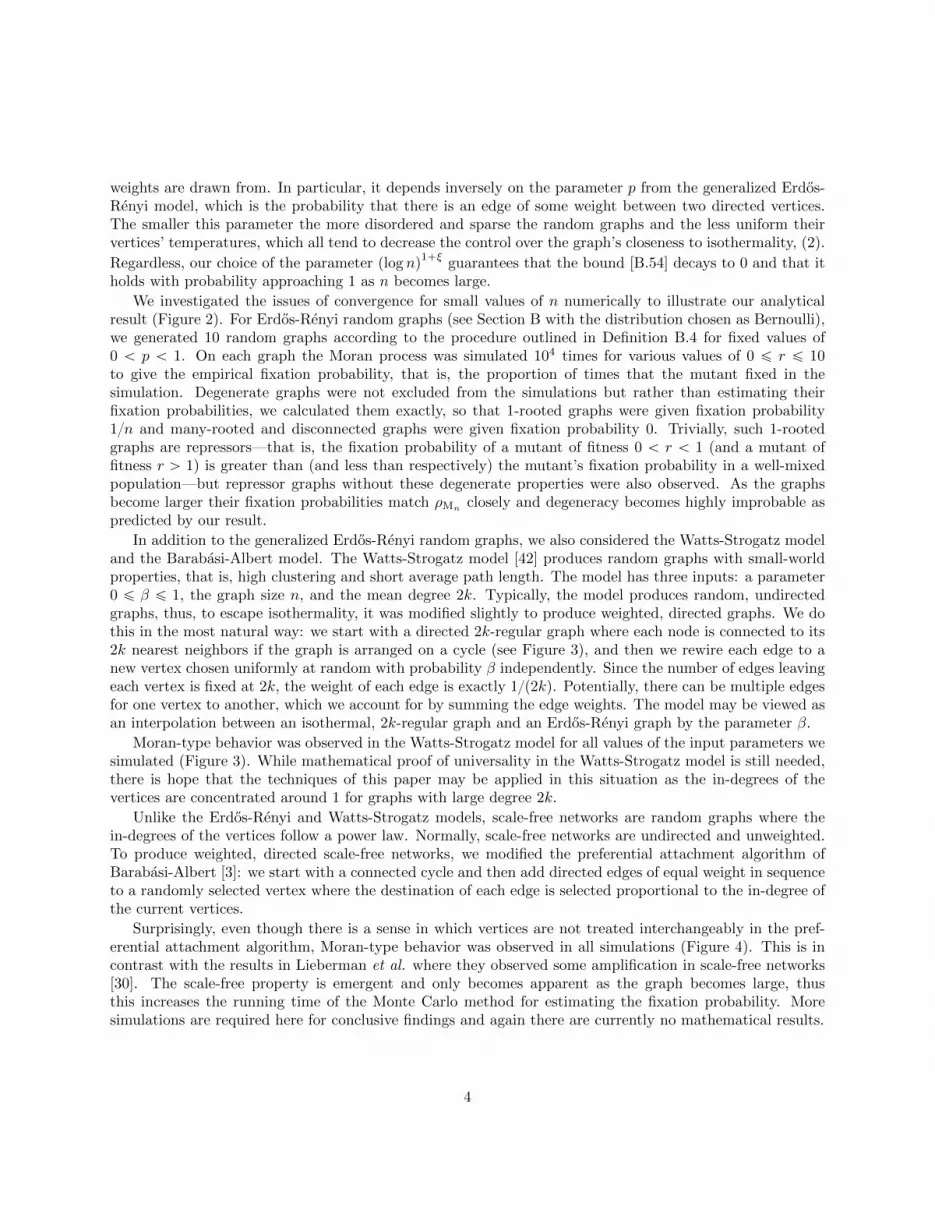
In addition to the generalized Erdos-Renyi random graphs, we also considered the Watts-Strogatz modeland the Barabasi-Albert model. The Watts-Strogatz model [42] produces random graphs with small-worldproperties, that is, high clustering and short average path length. The model has three inputs: a parameter0 ď β ď 1, the graph size n, and the mean degree 2k. Typically, the model produces random, undirectedgraphs, thus, to escape isothermality, it was modified slightly to produce weighted, directed graphs. We dothis in the most natural way: we start with a directed 2k-regular graph where each node is connected to its2k nearest neighbors if the graph is arranged on a cycle (see Figure 3), and then we rewire each edge to anew vertex chosen uniformly at random with probability β independently. Since the number of edges leavingeach vertex is fixed at 2k, the weight of each edge is exactly 1p2kq. Potentially, there can be multiple edgesfor one vertex to another, which we account for by summing the edge weights. The model may be viewed asan interpolation between an isothermal, 2k-regular graph and an Erdos-Renyi graph by the parameter β.

Moran-type behavior was observed in the Watts-Strogatz model for all values of the input parameters wesimulated (Figure 3). While mathematical proof of universality in the Watts-Strogatz model is still needed,there is hope that the techniques of this paper may be applied in this situation as the in-degrees of thevertices are concentrated around 1 for graphs with large degree 2k.

Unlike the Erdos-Renyi and Watts-Strogatz models, scale-free networks are random graphs where thein-degrees of the vertices follow a power law. Normally, scale-free networks are undirected and unweighted.To produce weighted, directed scale-free networks, we modified the preferential attachment algorithm ofBarabasi-Albert [3]: we start with a connected cycle and then add directed edges of equal weight in sequenceto a randomly selected vertex where the destination of each edge is selected proportional to the in-degree ofthe current vertices.

Surprisingly, even though there is a sense in which vertices are not treated interchangeably in the pref-erential attachment algorithm, Moran-type behavior was observed in all simulations (Figure 4). This is incontrast with the results in Lieberman et al. where they observed some amplification in scale-free networks[30]. The scale-free property is emergent and only becomes apparent as the graph becomes large, thusthis increases the running time of the Monte Carlo method for estimating the fixation probability. Moresimulations are required here for conclusive findings and again there are currently no mathematical results.

4

In summary, we have generalized the isothermal theorem to make it biologically realistic and to increaseits technical applicability. The conclusion of the robust isothermal theorem now depends continuously onits assumptions. With this new tool, we have proved analytically that fixation probabilities in a generalizedErdos-Renyi model converge uniformly to the fixation probability of a well-mixed population. In our proof,we identify the reason for this convergence and bound its rate. Thus, we confirm observations from manysimulations and give a method of approximation with a specified error. Furthermore, we conjecture thatmany random graph models exhibit this universal behavior. However, it is easy to construct simple examplesof random graphs which do not, thus it still remains to determine the necessary assumptions on the randomgraph model for it to exhibit universal behavior.

5

0 2 4 6 8 10

0.0

0.2

0.4

0.6

0.8

1.0

r

ΡG

HrL

0 2 4 6 8 10

0.0

0.2

0.4

0.6

0.8

1.0

r

ΡG

HrL

0 2 4 6 8 10

0.0

0.2

0.4

0.6

0.8

1.0

r

ΡG

HrL

0 2 4 6 8 10

0.0

0.2

0.4

0.6

0.8

1.0

r

ΡG

HrL

0.6

0.8

1.0

1.2

1.4

1 2 3 4 5

6 7 8 9 10

11 12 13 14 15

16 17 18 19 20

1 2 3 4 5

6 7 8 9 10

11 12 13 14 15

16 17 18 19 20

1 2 3 4 5

6 7 8 9 10

11 12 13 14 15

16 17 18 19 20

1 2 3 4 5

6 7 8 9 10

11 12 13 14 15

16 17 18 19 20

æ æ æ æ æ æ æ æ æ

æ

æ

æ

æ

æ

æ

æ

æ

æ

æ

æ

æ

æ

æ

æ

æ

æ

ææ

æ

æ

æ

ææ

æ æ

æ

ææ

ææ

æ

ææ æ

ææ æ

æ æ ææ æ

æ ææ

ææ

ææ æ

æ ææ æ

ææ æ

æ

æ æ æ æ ææ æ æ

æ æ æ æ ææ æ æ

æ æ æ ææ æ æ æ

æ ææ æ

æ ææ æ æ

æ æ æ æ æ æ æ æ æ

æ

æ

æ

æ

æ

æ

æ

æ

æ

æ

æ

æ

æ

æ

æ

æ

æ

ææ

æ æ

ææ

ææ æ

ææ

æ

æ

ææ

ææ æ

æ æ

æ ææ æ

æ æ ææ

ææ

æ ææ

æ æ ææ æ

æ

ææ æ

æ æ æ æ æ ææ

æ æ ææ æ

æ æ æ

æ ææ æ

æ æ ææ æ

ææ æ æ

æ æ æ ææ

æ æ æ æ æ æ æ æ æ

æ

æ

æ

æ

æ

æ

æ

æ

æ

æ

æ

æ

æ

æ

ææ

æ

æ

ææ

æ

æ

æ

æ æ ææ

æ æ æ æ

æ ææ

æ

æ

æ æ ææ æ

æ ææ

æ ææ

æ ææ æ

æ æ ææ æ

ææ

æ æ æ æ æ

ææ

ææ

æ ææ

æ æ ææ æ

ææ æ

æ æ æ ææ æ

æ æ æ æ æ æ

ææ

æ æ æ æ æ æ æ æ æ

æ

æ

æ

æ

æ

æ

æ

æ

æ

æ

æ

æ

æ

ææ

æ

æ

æ

ææ

æ

æ

æ

æ æ

ææ

ææ

æ æ

æ æ

æ ææ

ææ æ

ææ æ æ æ

æ æ æ ææ æ

ææ

æ ææ æ æ æ

æ æ æ æ ææ æ

æ æ ææ æ æ æ æ

æ æ ææ æ æ

æ æ ææ æ æ æ æ æ

ææ

æ æ

Ε=0.0

Ε=0.1

Ε=0.2

Ε=0.4

ΡMHrL

0 2 4 6 8 10

0.0

0.2

0.4

0.6

0.8

1.0

r

ΡG

HrL

æ æ æ æ æ æ æ æ æ

æ

æ

æ

æ

æ

æ

æ

æ

æ

æ

æ

æ

æ æ æ æ æ æ æ ææ

æ

æ

æ

æ

æ

æ

æ

æ

æ

æ

æ

æ

æ æ æ æ æ æ æ æ æ

æ

æ

æ

æ

æ

æ

æ

æ

æ

æ

æ

æ

æ æ æ æ æ æ æ æ æ

æ

æ

æ

æ

æ

æ

æ

æ

æ

æ

æ

æ

0.0 0.5 1.0 1.5 2.00.0

0.1

0.2

0.3

0.4

0.5

0.6

r

ΡG

HrL

0 2 4 6 8 10-0.02

-0.01

0.00

0.01

0.02

r

ΡG

HrL-

ΡM

HrLFigure 1: The robust isothermal theorem guarantees that the fixation probability of an approximately isother-mal graph lies in the green region and dashed lines indicate the optimal bound. As the perturbation strengthdecreases through ε P r0.4, 0.1s and the graph approaches isothermality, the bound improves and convergesuniformly to the solid black line, ρMn . The figures of square lattices show how random perturbations shiftthe graphs from isothermality, as the perturbation strength decreases from left to right; we draw each graphwith the directed edges’ thickness proportional to their weight and the vertices’ color given by the sum ofthe weights of edges pointing to them. In the bottom row empirical estimates of the fixation probabilities(small circles) are plotted against the values predicted by ρMn

(solid lines) and, despite the perturbations tothe graphs, their fixation probabilities lie close to ρMn .

6

0.0

0.5

1.0

1.5

2.0

n=5

n=7

n=10

n=20

0 2 4 6 8 10

0.0

0.2

0.4

0.6

0.8

1.0

r

ΡG

HrL

n=5

n=7

n=10

n=20

0 2 4 6 8 10

0.0

0.2

0.4

0.6

0.8

1.0

r

ΡG

HrL

n=5

n=7

n=10

n=20

0 2 4 6 8 10

0.0

0.2

0.4

0.6

0.8

1.0

r

ΡG

HrL

0.0 0.5 1.0 1.5 2.00.0

0.1

0.2

0.3

0.4

0.5

0.6

r

ΡG

HrL

0.0 0.5 1.0 1.5 2.00.0

0.1

0.2

0.3

0.4

0.5

0.6

r

ΡG

HrL

0.0 0.5 1.0 1.5 2.00.0

0.1

0.2

0.3

0.4

0.5

0.6

r

ΡG

HrL

0 2 4 6 8 10

-0.04

-0.02

0.00

0.02

0.04

r

ΡG

HrL-

ΡM

HrL

0 2 4 6 8 10

-0.04

-0.02

0.00

0.02

0.04

r

ΡG

HrL-

ΡM

HrL

0 2 4 6 8 10

-0.04

-0.02

0.00

0.02

0.04

r

ΡG

HrL-

ΡM

HrL

Figure 2: The fixation probability of the generalized Erdos-Renyi random graphs converge uniformly toρMn

. The three columns from left to right correspond to Erdos-Renyi random graphs with decreasingconnection probabilities p “ 1, p “ 0.6, and p “ 0.3. The representative random graphs in the top row showboth the increasing sparsity and disorder as p decreases and the elimination of degeneracy (rootedness anddisconnectedness) and the increasing uniformity of temperature as the graph sizes increase. In the middle tworows empirical estimates of the fixation probabilities (small circles) are plotted against the values predictedby ρMn

(solid lines). When p “ 1 the graphs are isothermal and thus correspond exactly to their predictedvalues which can be seen even more clearly in the bottom row, where the difference of the empirical fixationprobabilities and their predicted values display as stochastic fluctuations about 0. For p “ 0.6 and p “ 0.3,the convergence of the empirical values to ρMn as the graphs increases in size is apparent. Smaller graphsare typically repressors as illustrated by the clear sign change at r “ 1 in the difference of empirical andpredicted values, whereas larger graphs fluctuate about 0. Moreover, the convergence is patently slower inn for smaller values of p.

7

0.0

0.5

1.0

1.5

2.0

æ æ æ æ æ æ æ æ æ

æ

æ

æ

æ

æ

æ

æ

æ

æ

æ

æ

æ

æ

æ

æ

æ

æ

æ

æ

ææ

æ

æ

æ

ææ

ææ

æ æ

æ ææ

ææ æ

æ ææ

æ æ ææ æ

æ ææ æ

æ æ æ æ æ æ æ æ æ æ æ æ æ æ æ æ æ æ æ æ æ æ æ æ æ æ æ æ æ æ æ æ æ æ æ æ æ æ æ æ æ æ æ æ

æ æ æ æ æ æ æ æ æ

æ

æ

æ

æ

æ

æ

æ

æ

æ

æ

æ

æ

æ

æ

æ

æ

æ

æ

æ

æ

æ

ææ

ææ

ææ

ææ

ææ

ææ

ææ æ

æ ææ æ

ææ æ æ æ

æ ææ æ æ æ æ æ æ æ æ æ æ

æ æ æ æ æ æ æ æ æ æ æ æ æ æ æ ææ æ æ æ æ æ æ æ æ æ æ æ æ æ æ æ æ æ

æ æ æ æ æ æ æ æ æ

æ

æ

æ

æ

æ

æ

æ

æ

æ

æ

æ

æ

æ

æ

æ

æ

æ

æ

æ

æ

æ

æ

ææ

ææ

æ

ææ

ææ

ææ æ

ææ

æ ææ

æ ææ æ

ææ æ æ æ

æ ææ æ æ æ æ

æ æ æ æ æ ææ æ æ æ æ æ æ æ æ æ æ æ æ æ æ æ æ æ æ æ æ æ æ æ æ æ æ æ æ æ æ

æ æ æ æ æ æ æ æ æ

æ

æ

æ

æ

æ

æ

æ

æ

æ

æ

æ

æ

æ

æ

æ

æ

æ

ææ

æ

ææ

ææ

ææ

æ

ææ

ææ

ææ æ

æ ææ æ

æ æ æ ææ æ

æ æ æ æ ææ æ

æ æ æ æ æ æ æ æ æ æ ææ æ

æ æ æ æ æ æ æ æ æ æ æ æ æ æ æ æ æ æ æ æ æ æ æ æ æ æ æ æ

Β=0

Β=0.3

Β=0.6

Β=1

ΡMHrL

0 2 4 6 8 10

0.0

0.2

0.4

0.6

0.8

1.0

r

ΡG

HrL

æ æ æ æ æ æ æ æ æ

æ

æ

æ

æ

æ

æ

æ

æ

æ

æ

æ

æ

æ æ æ æ æ æ æ æ æ

æ

æ

æ

æ

æ

æ

æ

æ

æ

æ

æ

æ

æ æ æ æ æ æ æ æ æ

æ

æ

æ

æ

æ

æ

æ

æ

æ

æ

æ

æ

æ æ æ æ æ æ æ æ æ

æ

æ

æ

æ

æ

æ

æ

æ

æ

æ

æ

æ

0.0 0.5 1.0 1.5 2.00.0

0.1

0.2

0.3

0.4

0.5

0.6

r

ΡG

HrL

0 2 4 6 8 10-0.010

-0.005

0.000

0.005

0.010

r

ΡG

HrL-

ΡM

HrL

Figure 3: Small-world networks also show universal behavior. Representative Watts-Strogatz random graphsdisplay increasing disorder as the rewiring probability β increases from 0 to 1, which may be viewed asan interpolation between an isothermal graph to an Erdos-Renyi random graph. For all values of β thecorrespondence to ρMn

is striking but mathematical proof is lacking.

8

0.6

0.8

1.0

1.2

1.4

1.6

0.5 1.0 1.5

0.00

0.05

0.10

0.15

0.20

0.4

0.6

0.8

1.0

1.2

1.4

1.6

1.8

0.5 1.0 1.5 2.0

0.00

0.05

0.10

0.15

0.20

0.5

1.0

1.5

2.0

0.5 1.0 1.5 2.0

0.00

0.05

0.10

0.15

0.20

0.6

0.8

1.0

1.2

1.4

1.6

1.8

0.5 1.0 1.5 2.0

0.00

0.05

0.10

0.15

0.20

æ ææ

æ

æ

æ

æ

æ

æ

æ

æ

æ

ææ

ææ

ææ

æ ææ

æ æ

æ

æ

æ

æ

æ

æ

æ

æ

æ

ææ

æ

ææ

æ

æ ææ

æ

æ ææ

æ

æ

æ

æ

æ

æ

æ

æ

æ

æ

ææ

æ

æ ææ

æ æ

æ ææ

æ

æ

æ

æ

æ

æ

æ

æ

æ

æ

ææ

æ ææ

ææ æ

m=10

m=20

m=40

m=80

ΡMHrL

0 2 4 6 8 10

0.0

0.2

0.4

0.6

0.8

1.0

r

ΡG

HrL

æ æ æ æ æ æ æ æ æ æ

æ

æ

æ

æ

æ

æ

æ

æ

æ

æ

æ

æ æ æ æ æ æ æ æ æ æ

æ

æ

æ

æ

æ

æ

æ

æ

æ

æ

æ

æ æ æ æ æ æ æ æ æ æ

æ

æ

æ

æ

æ

æ

æ

æ

æ

æ

æ

æ æ æ æ æ æ æ æ æ æ

æ

æ

æ

æ

æ

æ

æ

æ

æ

æ

æ

0.0 0.5 1.0 1.5 2.00.0

0.1

0.2

0.3

0.4

0.5

0.6

r

ΡG

HrL

0 2 4 6 8 10-0.02

-0.01

0.00

0.01

0.02

r

ΡG

HrL-

ΡM

HrL

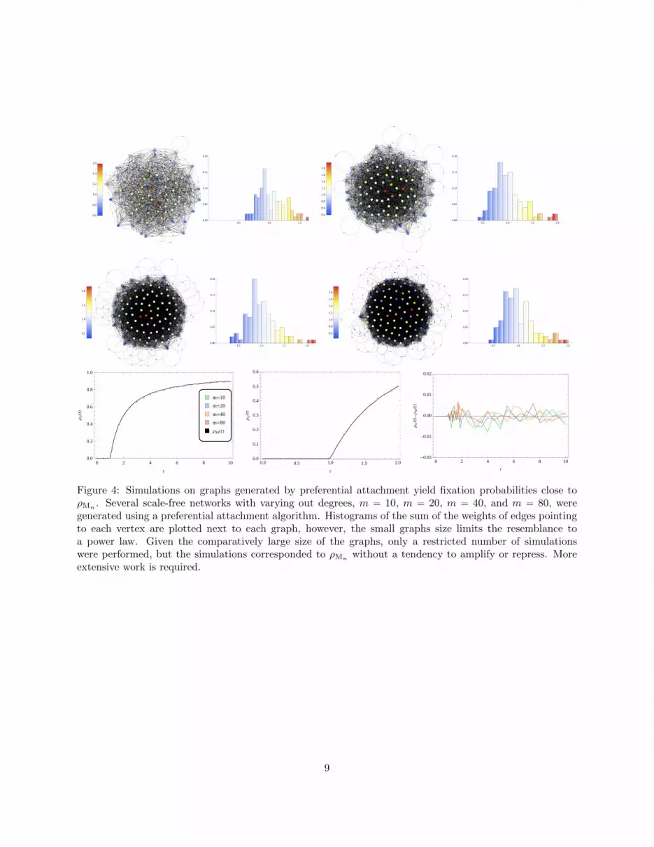
Figure 4: Simulations on graphs generated by preferential attachment yield fixation probabilities close toρMn . Several scale-free networks with varying out degrees, m “ 10, m “ 20, m “ 40, and m “ 80, weregenerated using a preferential attachment algorithm. Histograms of the sum of the weights of edges pointingto each vertex are plotted next to each graph, however, the small graphs size limits the resemblance toa power law. Given the comparatively large size of the graphs, only a restricted number of simulationswere performed, but the simulations corresponded to ρMn

without a tendency to amplify or repress. Moreextensive work is required.

9

Appendix A. The robust isothermal theorem

The Moran process on graphs is the standard model for population structure in evolutionary dynamics[30, 35]. The process is defined for a directed, weighted graph, G ” Gn “ pVn,Wnq, where V ” Vn :“ JnKand W ”Wn :“ rwijs is a stochastic matrix of edge weights. The process Xt is Markovian with state space2V , where each Xt is the subset of V consisting of all the vertices occupied by mutants at time t. At time 0a mutant is placed at one of the vertices uniformly at random or formally,

PrX0 “ Ss “

#

n´1 if |S| “ 1

0 otherwise. (A.1)

Then at each subsequent time step exactly one vertex is chosen randomly, proportional to its fitness, forreproduction: so the probability of choosing a particular wild type vertex is 1pn ´ |Xt| ` r|Xt|q and theprobability of choosing a particular mutant vertex is rpn ´ |Xt| ` r|Xt|q. An edge originating from thechosen vertex is then selected randomly with probability equal to its edge weight, which is well defined sinceW is stochastic, and the vertex at the destination of the edge takes on the type of the vertex at the originof the edge.

Typically, there are exactly two absorbing states, Xt “ H and Xt “ V , corresponding to the wild typefixing in the population and the mutant fixing in the population respectively. Thus, almost surely, one ofthese two absorbing states is reached in finite time. The probability that the process reaches V and not His called the fixation probability and for a graph G we denote its fixation probability for a mutant of fitnessr ą 0 by

ρGprq :“ PrXt “ V for some t ě 0s. (A.2)

A fundamental point of comparison is the fixation probability ρMnfor a well-mixed population structure,

where the graph structure is given by

wij :“

#

pn´ 1q´1 if i ‰ j

0 if i “ j(A.3)

and M stands for “Moran” or “mixed.” An easy calculation using recurrence equations shows that

ρMnprq “1´ r´1

1´ r´n. (A.4)

Graphs with exactly the same fixation probability as ρMn are classified by the isothermal theorem, whichgives sufficient conditions for a general graph G to have the same fixation probability as ρMn [30].

In this section we derive a generalization of the isothermal theorem and throughout we shall require thatthe matrix W is stochastic—that is, the row sums are all equal to 1:

nÿ

j“1

wij “ 1, (A.5)

for all i P V . Any graph with nonnegative edge weights can be normalized to produce a graph with astochastic W , so long as each row has a nonzero entry, without changing the behavior of the process as definedabove. A graph G is called isothermal if all the column sums of W are identical—that is, W1 “ ¨ ¨ ¨ “Wn “ 1,where

Wj :“nÿ

i“1

wij , (A.6)

10

or equivalently, W is doubly stochastic.For all S Ď V , define

wOpSq :“ÿ

iPS

ÿ

jRS

wij and wIpSq :“ÿ

iRS

ÿ

jPS

wij (A.7)

as the sum of the edge wights leaving S and entering S respectively. Then an easy calculation shows that agraph is isothermal if and only if

wOpSq “ wIpSq (A.8)

for all H ‰ S Ĺ V . The later condition and its equivalence to isothermality is at the core of the proof ofthe isothermal theorem. The term “isothermal” originates from an interpretation of the sum of the ingoingedge weights as temperature, with “hotter” vertices changing more frequently in the Moran process. Thus agraph satisfying (A.8) is isothermal because the ingoing and outgoing temperatures are equal and all subsetsS are in “thermal equilibrium.” We now restate the forward direction of the original isothermal theorem.

Theorem A.1 (Isothermal theorem). Suppose that a graph G is isothermal, then the fixation probabilityof a randomly placed mutant of fitness r is equal to ρMn

prq.

We ask, can we relax the assumptions of Theorem A.1? That is, perhaps an approximate result can beobtained for W that are only approximately doubly stochastic in the following sense:

|Wj ´ 1| ď ε (A.9)

for all j P V and some small quantity ε. However, the example

W “

»

—

—

–

0 1´ ε ε 01´ ε 0 0 εε2 0 0 1´ ε2

0 ε2 1´ ε2 0

fi

ffi

ffi

fl

(A.10)

shows we cannot, since as εÑ 0wOpt1, 2uq

wIpt1, 2uq“

2ε

2ε2“ ε´1 Ñ8. (A.11)

That is, W is approximately doubly stochastic, but the ratio of the outgoing and ingoing edge weights isunbounded for some subset S. Thus, we need stronger assumptions for our theorem which we state now.

Theorem A.2 (Robust isothermal theorem). Fix 0 ď ε ă 1. Let Gn “ pVn,Wnq be a connected graph.If for all nonempty S Ĺ Vn we have ∣∣∣∣wOpSq

wIpSq´ 1

∣∣∣∣ ď ε, (A.12)

thensuprą0

|ρMnprq ´ ρGnprq| ď ε. (A.13)

Proof. To briefly outline the proof, we begin by projecting the process from Xt to |Xt|. Next we considerthe ratio of the probability of increasing the number of mutants to the probability of decreasing the numberof mutants. By bounding this ratio we can use a coupling argument to establish that the fixation probabilityof the process is close to ρMn . Finally, we use the mean value theorem and smoothness properties of ρMn tosimplify our bound and obtain the result.

11

Just as in the proof of the original isothermal theorem, we make the projection of the state space ofall subsets of V , which records exactly which vertices are mutants, to the simpler state space t0, 1, . . . , nu,which records only the number of mutants. The problem with making this projection in general is that thetransition probabilities from one subset to another can depend on the structure of a subset not merely thenumber of mutants. However, it is clear that the only quantities which affect the fixation probability are theratios of the probability of increasing the number of mutants to the probability of decreasing the number ofmutants in a particular state S.

Define p`pSq and p´pSq as the probability that the number of mutants in a population increases anddecreases by one respectively. Thus

p`pSq “wOpSqr

wOpSqr ` wIpSqand p´pSq “

wIpSq

wOpSqr ` wIpSq, (A.14)

which gives, when the two equations are divided,

p`pSq

p´pSq“ r

wOpSq

wIpSq. (A.15)

By assumption (A.12),

rp1´ εq ďp`pSq

p´pSqď rp1` εq. (A.16)

This states that the ratio of the probabilities of increasing to decreasing the number of mutants in any stateS is approximately proportional to r.

If for some graph G1 “ pV 1,W 1q we have p`pSqp´pSq “ rp1 ˘ εq for all S Ď V 1, then by the standardresult for fixation probabilities in birth-death processes, its fixation probability is given by

ρG1prq “ ρMnpr ˘ rεq “

1´ pr ˘ εrq´1

1´ pr ˘ εrq´n. (A.17)

From (A.16) and (A.17) we would like to conclude that

ρMnpr ´ rεq “

1´ pr ´ εrq´1

1´ pr ´ εrq´nď ρGprq ď

1´ pr ` εrq´1

1´ pr ` εrq´n“ ρMn

pr ` rεq. (A.18)

The upper bound is given by taking the maximum allowed value for the probability of increasing the numberof mutants relative to the probability of decreasing the number of mutants. For the lower bound we use theopposite.

This intuitive result can be proved with a coupling argument. We can couple the Moran process Xt ofa mutant of fitness r on G with another process Y defined as follows: Y has state space t0, . . . , nu (with 0and n absorbing) and Y starts at 1. We couple Y to Xt as follows:

(i) if |Xt| decreases by 1, then Y must also decrease by 1;

(ii) if |Xt| increases by 1, then independently Y increases by 1 with probability

P`pSq ` P´pSq

P`pSq

rp1´ εq

1` rp1´ εq(A.19)

(which is less than or equal to 1 by assumption (A.16)), else Y decreases by 1;

12

(iii) otherwise Y remains constant.

Note that marginally Y is a simple random walk on t0, . . . , nu with forward bias rp1 ´ εq and thus theprobability that Y reaches n before it reaches 0 is given by

1´ pr ´ εrq´1

1´ pr ´ εrq´n. (A.20)

However, because the processes are coupled we have Y ď |Xt| and thus if Y “ n, then the mutant has fixedin the process Xt. Equation (A.20) immediately implies the lower bound in (A.18). A similar coupling yieldsthe upper bound. Thus

ρMnpr ´ rεq ´ ρMn

prq ď ρGprq ´ ρMnprq ď ρMn

pr ` rεq ´ ρMnprq. (A.21)

By the mean value theorem,

ρMnpr ` rεq ´ ρMn

prq

εďrε

εsup

rďxďr`rε

∣∣ρ1Mnpxq

∣∣ “ r suprďxďr`rε

∣∣ρ1Mnpxq

∣∣ (A.22)

andρMnprq ´ ρMnpr ´ rεq

εě ´r sup

r´rεnďxďr

∣∣ρ1Mnpxq

∣∣ . (A.23)

Thus, it is sufficient to show for all r ą 0

supně2

∣∣ρ1Mnprq

∣∣ ď r´1. (A.24)

We note that this is not an optimal bound, however, it sufficies for our applications. Calculating, one finds

ρ1Mnprq “

rn´2 prn ´ nr ` n´ 1q

prn ´ 1q2 . (A.25)

First, when r ě 1 we prove the stronger claim

rn´2 prn ´ nr ` n´ 1q

prn ´ 1q2 ď r´2, (A.26)

by noting the above is equivalent to

pr ´ 1q

˜

nrn ´n´1ÿ

k“0

rk

¸

ě 0, (A.27)

which is true since r ě 1. Similarly, one can prove

rn´2 prn ´ nr ` n´ 1q

prn ´ 1q2 ă 1 (A.28)

when r ă 1. Equations (A.26) and (A.28) imply supně2

∣∣ρ1Mnprq

∣∣ ď r´1.Therefore, we may conclude

suprą0

|ρGprq ´ ρMnprq| ď ε, (A.29)

which completes the proof.

13

Note that one can sometimes do slightly better (depending on the relative sizes of ε and n´1), by showing

suprď1

|ρGnprq ´ ρMnprq| ă2

n(A.30)

for ε small enough, using the triangle inequality and the facts that ρMnis increasing and continuous, but

again this is not important for our applications.

Theorem A.2 is actually slightly stronger than stated, and thus we can draw a slightly stronger conclusionin Theorem B.1. We may conclude that the fixation probability of a mutant of fitness r originating at aparticular vertex i [2] satisfies the bound in (A.13), for exactly the same reason as in the proof of the originalisothermal theorem—the bound (A.12) is for all subsets S. Therefore, a fortiori, a mutant can be startedwith any probability vector on the vertices (not merely uniform) and its fixation probability will still satisfy(A.13). This observation is borne through simulations too (Figure 5).

-----------

-

-

-

-

-

-

-

--

--

---

--

----

-------

---------------------------------------------------------------

----------

-

-

-

-

-

-

-

-

--

--

--

--

----

-----------------------------------------------------------------------

0 2 4 6 8 100.0

0.2

0.4

0.6

0.8

1.0

r

ΡG

HrL

Figure 5: Fixation probability does not depend on starting location. We conducted trials where the fixationprobability of a mutant of fitness r starting at vertex i was estimated with the Monte Carlo method of 104

samples for several values of 0 ď r ď 10 on a Erdos-Renyi random graph. The fixation probability wassimilar regardless of starting vertex, and in particular, showed no correlation with vertex temperature. Weplot the Moran fixation probability (A.4) and use the error bars to illustrate the minimum and maximumempirical fixation probabilities obtained from starting at any particular vertex.

Appendix B. Evolution on random graphs

In this section we prove Theorem B.1.

Theorem B.1. Let pGnqně1 be a family of random graphs as in Definition B.4. Then there are constantsC ą 0 and c ą 0, not dependent on n, such that the fixation probability of a randomly placed mutant offitness r ą 0 satisfies

|ρGnprq ´ ρMnprq| ď C plog nq

C`Cξ

?n

(B.1)

14

uniformly in r with probability greater than

1´ exp´

´ν plog nq1`ξ

¯

, (B.2)

for positive constants ξ and ν.

To do this we need to apply Theorem A.2 to our random graphs by showing that its assumptions holdwith high probability. We do so in several steps. First, we define precisely generalized Erdos-Renyi randomgraphs in Definition B.4 and outline the necessary assumptions on the distribution of the edge weights.After reviewing some notation, we introduce an event Ω, on which the graphs are well behaved, and showthat Ω has high probability in Lemma B.6. Then the general idea is to use large deviation estimates andconcentration inequalities to show that with high probability the quantity (A.12) can be controlled. Webound both the numerator (Lemma B.7) and denominator (Lemma B.8) of

|wOpSq ´ wIpSq||wIpSq|

“

∣∣∣∣wOpSq

wIpSq´ 1

∣∣∣∣ (B.3)

for all S, then we put everything together to prove Theorem B.1.

Remark B.2 (Notation). We use the large constant C ą 0 and the small constant c ą 0, which do notdepend on the size of the graph n but can depend on the distribution as outlined in Definition B.4. We allowthe constant C to increase or the constant c to decrease from line to line without noting it or introducing anew notation, sometimes we even absorb other constants such as p, p1, and µ1 without noting it; as is clearfrom the proof, this only happens a finite number of times, and thus we end with constants C ą 0, c ą 0,ν ą 0, and ξ ą 0.

We also make use of standard order notation for functions, op¨q, Op¨q, and ¨ " ¨, all of which are usedwith respect to n. Moreover, in some sums it is useful to exclude particular summands, e.g.

ÿ

1ďjďnjRS

¨ ”

pSqÿ

j

¨ (B.4)

for S Ă V . We abbreviate ptiuq and pti, kuq as piq and pi, kq.

Remark B.3 (High probability events). We say that an n-dependent event E holds with high probabilityif, for constants ξ ą 0 and ν ą 0 which do not depend on n,

PrEcs ď e´νplognq1`ξ

(B.5)

for n ě n0 pν, ξq. Moreover, we say an event E has high probability on another event E0 if

PrE0 X Ecs ď e´νplognq

1`ξ

(B.6)

In particular, this has the property that the intersection of polynomially many (in n, say KnK for someconstant K ą 0) events of high probability is also an event of high probability: by the union bound,

P

»

–

¨

˝

KnKč

i“1

Ei

˛

‚

cfi

fl “ P

»

–

KnKď

i“1

Eci

fi

fl ď KnK ¨ e´νplognq1`ξ

“ KeK logn´νplognq1`ξ ď e´νplognq1`ξ

, (B.7)

with a possible increase in n0 pν, ξq and a decrease in the constants ν and ξ.

15

B.1. Proof of Theorem B.1. Following the Erdos-Renyi model, we produce a weighted, directed graph asfollows: Consider an nˆ n matrix X “ rxijs with zero for its diagonal entries and independent, identicallydistributed, nonnegative random variables for its off-diagonal entries. We now want to define a random,stochastic matrix W of weights. The natural definition for W “ rwijs is

wij :“xij

řnk“1 xij

, (B.8)

which is defined when at least one of the xi1, . . . , xin is nonzero; this happens almost surely in the limit asnÑ8, when Prxij ą 0s “ p ą 0 is a constant:

Prxi1 “ xi2 “ ¨ ¨ ¨ “ xin “ 0s “ p1´ pqn´1 (B.9)

and by the union bound

P

«

nł

i“1

xi1 “ xi2 “ ¨ ¨ ¨ “ xin “ 0

ff

ď

nÿ

i“1

Prxi1 “ xi2 “ ¨ ¨ ¨ “ xin “ 0s “ np1´ pqn´1 Ñ 0. (B.10)

However, the question is how to technically deal with the unusual event that all the entries of a row ofX are zero, as there are several options. We make the following choice: for 1 ď i ď n

wii :“

#

1 if xi1 “ xi2 “ ¨ ¨ ¨ “ xin “ 0

0 otherwise, (B.11)

and for all 1 ď i, j ď n and i ‰ j

wij :“

#

xijřnk“1 xik

if xij ą 0

0 if xij “ 0. (B.12)

This definition aligns with the definition in (B.8) with probability greater than 1´np1´pqn. Moreover, thisdefinition has the advantage that the events that any non-loop edge weight is 0 are independent.

Definition B.4 (Generalized Erdos-Renyi random graphs). Let µ be a nonnegative distribution (notdepending on n) with subexponential decay such that if X „ µ

PrX ą 0s “ p ą 0 and P rX ě xs ď Ce´xc

(B.13)

for some positive constants p, c, and C and all x ą 0. We denote the mean and standard deviation of X byµ1 and σ respectively. We generate a family of random graphs Gn “ pVn,Wnq from µ by defining the weightmatrices Wn according to (B.11) and (B.12), where xij are independent and distributed according to µ fori ‰ j.

The subexponential decay is necessary to control the fluctuation of the graph’s edge weights and imposesa bounded increase on the moments of µ. Let X „ µ, then simple calculations show,

µk :“ EXk ď Ck

ż 8

0

xk´1PrX ě xsdx ď Ck

ż 8

0

xk´1e´xc

dx “C

ckΓ

ˆ

1` k

c

˙

ď pCkqCk, (B.14)

where the constant C ą 0 depends on the constants in (B.13). Many distributions satisfy the subexponentialassumption (B.13), for example any compactly supported distribution, the Gamma distribution, and theabsolute value of a Gaussian distribution.

We now use the subexponential decay assumption to understand the typical behavior of the randomvariables xij .

16

Definition B.5 (Good events Ω). Let Ω be an n-dependent event such that the following hold:

Ω :“nč

i“1

¨

˝txii “ 0u X

$

&

%

∣∣∣∣∣∣piqÿ

j

pxij ´ Exijq

∣∣∣∣∣∣ ď σ plog nqC`Cξ?

n

,

.

-

˛

‚ (B.15)

X

nč

i,j“1

!

xij ď C plog nqC)

X tGn is connectedu . (B.16)

The conditions on Ω have natural interpretations. The first condition specifies that the normalizationprocedure outlined above has worked as intended and that we are not in the atypical case where the graphhas a self-loop. The second condition specifies that the sums of n of the xijs are close to their expectationpn ´ 1qµ1 and that they fluctuate about this value on the order of

?n as predicted by the central limit

theorem. The third condition says that none of the xij are too large and that typically they will all be less

than C plog nqC

. The last condition is self-explanatory, as the Moran process is not guaranteed to terminateon disconnected graphs.

Lemma B.6. The event Ω holds with high probability.

Proof. By Remark B.3, it suffices to show that each conjunct holds with high probability as there are onlypolynomially many choices for i and j. First fix i. By assumption (B.13) and the fact that xii ‰ 0 only ifxij “ 0 for all j ‰ i,

P txii ‰ 0u “ P rxij “ 0 for all j ‰ is ď p1´ pqn´1 “ elogp1´pqpn´1q ď e´νplognq1`ξ

, (B.17)

since 0 ă p ă 1 and n´ 1 " plog nq1`ξ.Now using the large deviation result, Lemma E.4, with aj “ xij ´ Exij and Aj “ 1, we may verify the

moment assumption (E.7): clearly E pxij ´ Exijq “ 0 and E pxij ´ Exijq2 “ σ2, then

E |xij ´ Exij |k ď pCkqCk (B.18)

by Equation (B.14). Thus we get

P

«∣∣∣∣∣ nÿi“1

aiAi

∣∣∣∣∣ ě σ plog nqC`Cξ?

n

ff

ď e´νplognq1`ξ

. (B.19)

Now fix j too. Next, we use the subexponential decay assumption (B.13) with x “ C plog nqC

forC “ 1` c´1 to get

P”

xij ą C plog nqc´1

`1ı

ď C exp´

´

´

C plog nqc´1

`1¯c¯

ď Ce´Ccplognq1`c ď e´νplognq

1`ξ

. (B.20)

Thus, xij ą C plog nqC

holds with high probability since c ą 0 and Cc ą 0.Finally, we show that the graph G is connected with high probability, i.e. that with high probability,

the graph cannot be partitioned into two disjoint sets where there are no edges going from one subset toanother. This follows from an argument similar to that contained in the proof of Lemma B.8 but withoutthe assumption that we are on the event Ω as we do not need a lower bound on the weights only that edgesexist which they do with probability at least p.

17

Note that by definition W is stochastic. Define the sum of the jth column as

Wj :“nÿ

i“1

wij . (B.21)

Note that while the family Wj is not independent, by symmetry, they are identically distributed. Hence

EW1 “1

n

nÿ

j“1

EWj “1

nE

nÿ

j“1

nÿ

i“1

wij “ 1. (B.22)

This tells us that in expectation W is doubly stochastic. The next lemma shows that with very highprobability it is almost n´12 close to being doubly stochastic, which is exactly the order of fluctuation weexpect by the central limit theorem. The assumptions on the distribution µ and the event Ω guarantee thatwe can prove that the sum’s fluctuations are of this order.

The idea of the proof is that for fixed j, the wij are independent random variables and thus we can applya lde to bound the fluctuations of their sum. There are complications due to the normalization requiredby Definition B.4 but on Ω these can be overcome by relating the sum Wj to a simpler sum that may becontrolled with Lemma E.4.

Lemma B.7. On Ω, there are positive constants c ” cµ and C ” Cµ, not dependent on n, such that thefollowing inequalities hold

|Wj ´ 1| ď C plog nqC`Cξ

?n

(B.23)

for all j P V , with probability at least

1´ e´νplognq1`ξ

. (B.24)

Proof. Fix j. First we use the fact that wii “ xii “ 0 for 1 ď i ď n on Ω to see

Wj ´ 1 “ÿ

i

pwij ´ Ewijq “pjqÿ

i

ˆ

wij ´1

n´ 1

˙

`O`

n2p1´ pq´n`1˘

. (B.25)

By the definition of wij , the above is equal to

pjqÿ

i

˜

xijřpiqk xik

´1

n´ 1

¸

`O`

c´n0

˘

“

pjqÿ

i

˜

xij ´1

n´1

řpiqk xik

řpiqk xik

¸

`O`

c´n0

˘

, (B.26)

where c0 ă 1 is not dependent on n. Next, using the fact that on Ω

1

n´ 1

∣∣∣∣∣∣piqÿ

k

pxik ´ Exikq

∣∣∣∣∣∣ ď Cσ plog nqC`Cξ 1

?n

(B.27)

for all 1 ď i ď n, we replace the average in the numerator of (B.26) with its expectation to find it equal to

pjqÿ

i

˜

xij ´ Exijřpiqk xik

`Cσ plog nq

C`Cξ

?nřpiqk xik

¸

`O`

c´n0

˘

. (B.28)

18

Using (B.27) again, it is easy to see

piqÿ

k

xik ě pn´ 1qExij ´ Cσ plog nqC`Cξ?

n, (B.29)

which gives an upper bound on the error term in (B.28) and we find the equation equal to

pjqÿ

i

xij ´ Exijřpiqk xik

`O

˜

plog nq2C`2Cξ

?n

¸

`O`

c´n0

˘

. (B.30)

Next we compare these two expressions to find that the absolute value their difference can be expressed as∣∣∣∣∣xij ´ Exijřpiqk xik

´xij ´ Exijřpi,jqk xik

∣∣∣∣∣ “ |xij |2∣∣∣řpiqk xik ¨´

řpiqk xik ´ xij

¯∣∣∣ . (B.31)

However, using that on Ω, for all 1 ď i, j ď n, we have xij ď C plog nqC

and using (B.27) as before, we mayshow the difference is bounded by

O

˜

plog nq4C`2Cξ

n2

¸

. (B.32)

We can then sum over these errors—one for each summand—to get a total error of O´

plog nq4C`2Cξ

n¯

.

Thus, (B.30) may be rewritten as

pjqÿ

i

xij ´ Exijřpi,jqk xik

`O

˜

plog nq2C`2Cξ

?n

¸

, (B.33)

since the other error terms are dominated by the remaining one.Note that xij does not appear in the summand’s denominator and thus the denominator and numerator

are independent. So we can use the large deviation estimate, Lemma E.4, with ai “ xij ´ Exij and

A´1i “

řpi,jqk xik. While the Ai are random, we may condition on their values and treat them as deterministic

constants, then after we have used the lde, we can bound them using the fact that we are on Ω. That is,on Ω

¨

˝

pi,jqÿ

k

xik

˛

‚

2

“ pn´ 2q2 pExijq2 `O´

plog nq2C`2Cξ

n?n¯

(B.34)

and sopjqÿ

k

A2i “

1

pn´ 2q pExijq2`O

ˆ

plog nq2C`2Cξ 1

n?n

˙

. (B.35)

Thus the lde gives us

P

»

–

∣∣∣∣∣∣pjqÿ

i

aiAi

∣∣∣∣∣∣ ě C plog nqC`Cξ

?n

fi

fl ď e´νplognq1`ξ

, (B.36)

19

which combined with (B.33)

P

«

|Wj ´ 1| ě C plog nq2C`2Cξ

?n

ff

ď e´νplognq1`ξ

. (B.37)

The properties of high probability and the fact that we have n choices for j completes the proof.

Next we prove a lower bound on sums of edge weights, wIpSq and wOpSq for all H ‰ S Ĺ Vn. The proofrelies on concentration inequalities for independent random variables and the simple fact that on Ω there isa constant c ą 0 such that wij ě cn´1

1 pxij ě cq for all i, j P V .

Lemma B.8. On Ω, for all H ‰ S Ĺ Vn and some small constant c ” cµ ą 0, not dependent on n, we havethe following bound

|wIpSq| “ |wOpScq| ě cµ min t|S|, n´ |S|u (B.38)

with probability greater than

1´ e´νplognq1`ξ

. (B.39)

Proof. First note that as in the proof of Lemma B.7, we can argue that on Ω the sumřpiqk xik ď Cn, see

(B.29) for all 1 ď i ď n. Moreover, by assumption on the distribution µ, we have P rxij ą 0s “ p ą 0 andthus there is a constant c ą 0 such that P rxij ě cs “ p1 ą 0. Therefore, on Ω

wij ě cn´11 pxij ě cq . (B.40)

However, for each 1 ď i, j ď n with i ‰ j, define βij :“ 1 pxij ě cq which are independent Bernoulli randomvariables such that

Pr1 pxij ě cq “ 1s “ p1 ą 0, (B.41)

since the xij are independent.Let |S| “ k. By definition

wIpSq “ÿ

iRS

ÿ

jPS

wij “ wOpScq. (B.42)

Note that no diagonal terms are in these sums. Using (B.41),

ÿ

iPS

ÿ

iRS

wij ěc

n

ÿ

iPS

ÿ

iRS

βij . (B.43)

Note that now this is a sum of kpn ´ kq independent random variables. So for fixed H ‰ S Ĺ Vn, by theChernoff bound, Lemma E.3, the event

AS :“

#

ÿ

iPS

ÿ

iRS

βij ď p1´ 12qp1kpn´ kq

+

(B.44)

has probability less than

exp

ˆ

´1

8p1kpn´ kq

˙

. (B.45)

20

Thus, by the union bound

P

«

č

H‰SĹVn

AcS

ff

“ 1´ P

«

ď

H‰SĹVn

AS

ff

ě 1´ÿ

H‰SĹVn

P rASs

“ 1´n´1ÿ

k“1

ˆ

n

k

˙

P rASs

“ 1´

tlognuÿ

k“1

ˆ

n

k

˙

P rASs ´n´tlognu´1

ÿ

k“tlognu`1

ˆ

n

k

˙

P rASs ´n´1ÿ

n´tlognu

ˆ

n

k

˙

P rASs

ě 1´ 2nlogn exp`

´p1n8˘

´ 2n exp`

´p1n plog nq 8˘

ě 1´ 2 exp`

´`

p1n8´ plog nq2˘˘

´ exp`

´`

p1 log n8´ log 2˘

n˘

ě 1´ exp`

´cp1n˘

,

(B.46)

for some c ą 0. Finally, notecp1

2nkpn´ kq ě

cp1

2min t|S|, n´ |S|u (B.47)

andexpp´cp1nq ď e´νplognq

1`ξ

(B.48)

for an appropriate choice of ξ and ν.

We now complete the proof of Theorem B.1 by putting together the results of Section A and the lemmatafrom this section.

Proof of Theorem B.1. Again let |S| “ k. We check that the assumptions of Theorem A.2 hold withhigh probability. Observe ∣∣∣∣wOpSq

wIpSq´ 1

∣∣∣∣ “ ∣∣∣∣wOpSq ´ wIpSq

wIpSq

∣∣∣∣ “ |wOpSq ´ wIpSq||wIpSq|

. (B.49)

Expanding the numerator, we get

wOpSq ´ wIpSq “ÿ

iPS

ÿ

jRS

wij ´ÿ

iRS

ÿ

jPS

wij “ÿ

iPS

ÿ

jPV

wij ´ÿ

iPV

ÿ

jPS

wij “ÿ

jPS

p1´Wjq, (B.50)

and similarly,wOpSq ´ wIpSq “

ÿ

iPV

ÿ

jRS

wij ´ÿ

iRS

ÿ

jPV

wij “ÿ

jRS

pWj ´ 1q. (B.51)

Thus Lemma B.7 implies

|wOpSq ´ wIpSq| ď min tk, n´ ku ¨C plog nq

C`Cξ

?n

, (B.52)

for all S with high probability on Ω.

21

Lemma B.8 implies|wIpSq| ě cmin t|S|, n´ |S|u (B.53)

for all S with high probability on Ω. Putting this together we see∣∣∣∣wOpSq

wIpSq´ 1

∣∣∣∣ ď C plog nqC`Cξ

?n

(B.54)

for all S with high probability on Ω. However, by Lemma B.6, the event Ω holds with high probability itselfand thus unconditionally (B.54) holds for all S with high probability.

Finally, applying Theorem A.2, we get

suprą0

|ρGnprq ´ ρMnprq| ď C plog nq

C`Cξ

?n

(B.55)

with high probability.

Remark B.9 (On Theorem B.1). The parameter p, the probability that an edge of some weight existsbetween two directed vertices, can be interpreted as a measure of the sparseness of the population structure.We can ask how few interactions on average can individuals in a population have with others and still yieldpopulations with Moran-type behavior? While p can be arbitrarily small, we have kept it constant and, inparticular, not dependent on n. However, could p depend on n such that pÑ 0 as nÑ8 and still producegraphs which show Moran-type behavior? An obvious lower bound on the rate of p’s convergence to 0 isprovided by the Erdos-Renyi model, which tells us that a graph is almost surely disconnected in the limitfor

?p ă p1 ´ εqp1nq log n for any ε ą 0. This bound follows by noting that p1 ´ pq2 is the probability

that there is no edge, in either direction, between two vertices and then applying the usual Erdos-Renyithreshold [18, 12]. There is much room between this lower bound and p constant—even whether such asharp threshold for p exists is currently unclear. The issue is difficult to approach with naive simulations asthe Moran process is not guaranteed to terminate on disconnected graphs.

Appendix C. Graphs without outgoing weights summing to 1

The Moran process on graphs may be generalized to no longer require the sum of the outing going weightsof each vertex to be 1. The process is still defined for a directed, weighted graph, G ” Gn “ pVn,Wnq, whereV ” Vn :“ JnK but W ”Wn :“ rwijs need not be a stochastic matrix (it must still have nonnegative entries).Instead of sampling vertices proportional to fitness and then choosing an outgoing edge with probability equalto its weight, we rather sample edges proportional to their weights and the fitness of the individual at thebeginning of the edge. Once we select an edge the type of the individual at the end of the edge becomes thesame as the individual at the beginning of the edge. It is easy to see that we get the original process as aspecial case of the new model. Again, the process Xt is Markovian with state space 2V , where each Xt isthe subset of V consisting of all the vertices occupied by mutants at time t. At time 0 a mutant is placed atone of the vertices uniformly at random. We then update as described above by choosing edges proportionalto their weights and the individual’s type at the edges origin. For example, the probability of choosing aparticular edge pi, jq is

pr1iPXt ` 1iRXtqwijrř

iPXt

ř

jPV wij `ř

iRXt

ř

jPV wij. (C.1)

In this setting the robust isothermal theorem still holds.

22

Theorem C.1 (Robust isothermal theorem). Fix 0 ď ε ă 1. Let Gn “ pVn,Wnq be a connected graph.If for all nonempty S Ĺ Vn we have ∣∣∣∣wOpSq

wIpSq´ 1

∣∣∣∣ ď ε, (C.2)

thensuprą0

|ρMnprq ´ ρGnprq| ď ε. (C.3)

Proof. Just as before, we make the projection of the state space of all subsets of V , which records exactlywhich vertices are mutants, to the simpler state space t0, 1, . . . , nu, which records only the number of mutants.In the new model, we still have

p`pSq

p´pSq“ r

wOpSq

wIpSq. (C.4)

So the argument is exactly the same as the previous case.

Appendix D. More random graphs

We can introduce a random graph model where the sum of the outgoing weights are not equal, that is, whereindividuals can contribute differentially to the next time point in a way not dependent on the genotype theycarry. We change the model by not normalizing the outgoing edge weights. Following the Erdos-Renyi model,we produce a weighted, directed graph as follows: Consider an n ˆ n matrix X “ rxijs with independent,identically distributed, nonnegative random variables for its entries. Since we do not need to normalize wetake, W “ X.

Definition D.1 (Generalized Erdos-Renyi random graphs). Let µ be a nonnegative distribution (notdepending on n) with subexponential decay such that if X „ µ

PrX ą 0s “ p ą 0 and P rX ě xs ď Ce´xc

(D.1)

for some positive constants p, c, and C and all x ą 0. We denote the mean and standard deviation of X byµ1 and σ respectively. We generate a family of random graphs Gn “ pVn, Xn ” Wnq from µ, where xij areindependent and distributed according to µ.

Now we have a similar theorem to before but the proof is easier.

Theorem D.2. Let pGnqně1 be a family of random graphs as in Definition D.1. Then there are constantsC ą 0 and c ą 0, not dependent on n, such that the fixation probability of a randomly placed mutant offitness r ą 0 satisfies

|ρGnprq ´ ρMnprq| ď C plog nq

C`Cξ

?n

(D.2)

uniformly in r with probability greater than

1´ exp´

´ν plog nq1`ξ

¯

, (D.3)

for positive constants ξ and ν.

23

D.1. Proof of Theorem D.2. We now use the subexponential decay assumption to understand the typicalbehavior of the random variables xij .

Definition D.3 (Good events Ω). Let Ω be an n-dependent event such that the following hold:

Ω :“nč

i,j“1

!

xij ď C plog nqC)

X tGn is connectedu . (D.4)

Lemma D.4. The event Ω holds with high probability.

Proof. Identical to the previous proof.

Define the sum of the jth column as

Wj :“nÿ

i“1

wij (D.5)

and the sum of the ith row as

Wi :“nÿ

j“1

wij . (D.6)

Lemma D.5. On Ω, there are positive constants c ” cµ and C ” Cµ, not dependent on n, such that thefollowing inequalities hold

|Wj ´ µn| ď C plog nqC`Cξ?

n (D.7)

and ∣∣∣Wi ´ µn∣∣∣ ď C plog nq

C`Cξ?n (D.8)

for all i, j P V , with probability at least

1´ e´νplognq1`ξ

. (D.9)

Proof. Consider ai “ wij ´ µ or ai “ wji ´ µ and apply Lemma E.4. The claim follows immediately asthere are 2n high probability events.

Lemma D.6. On Ω, for all H ‰ S Ĺ Vn and some small constant c ” cµ ą 0, not dependent on n, we havethe following bound

|wIpSq| “ |wOpScq| ě cµ|S| pn´ |S|q (D.10)

with probability greater than

1´ e´νplognq1`ξ

. (D.11)

Proof. By assumption on the distribution µ, we have P rxij ą 0s “ p ą 0 and thus there is a constant c ą 0such that P rxij ě cs “ p1 ą 0. Define βij :“ 1 pxij ě cq which are independent Bernoulli random variablessuch that

Prβij “ 1s “ p1 ą 0, (D.12)

since the xij are independent. Let |S| “ k. By definition

wIpSq “ÿ

iRS

ÿ

jPS

xij “ wOpScq. (D.13)

24

Using (B.41),ÿ

iPS

ÿ

iRS

xij ě cÿ

iPS

ÿ

iRS

βij . (D.14)

Note that now this is a sum of kpn ´ kq independent random variables. So for fixed H ‰ S Ĺ Vn, by theChernoff bound, Lemma E.3, the event

AS :“

#

ÿ

iPS

ÿ

iRS

βij ď p1´ 12qp1kpn´ kq

+

(D.15)

has probability less than

exp

ˆ

´1

8p1kpn´ kq

˙

. (D.16)

Thus, by the union bound

P

«

č

H‰SĹVn

AcS

ff

“ 1´ P

«

ď

H‰SĹVn

AS

ff

ě 1´ÿ

H‰SĹVn

P rASs

“ 1´n´1ÿ

k“1

ˆ

n

k

˙

P rASs

“ 1´

tlognuÿ

k“1

ˆ

n

k

˙

P rASs ´n´tlognu´1

ÿ

k“tlognu`1

ˆ

n

k

˙

P rASs ´n´1ÿ

n´tlognu

ˆ

n

k

˙

P rASs

ě 1´ 2nlogn exp`

´p1n8˘

´ 2n exp`

´p1n plog nq 8˘

ě 1´ 2 exp`

´`

p1n8´ plog nq2˘˘

´ exp`

´`

p1 log n8´ log 2˘

n˘

ě 1´ exp`

´cp1n˘

,

(D.17)

for some c ą 0. Finally, note

expp´cp1nq ď e´νplognq1`ξ

(D.18)

for an appropriate choice of ξ and ν.

We now complete the proof of Theorem D.2.

Proof of Theorem D.2. Again let |S| “ k. We check that the assumptions of Theorem C.1 hold withhigh probability. Observe ∣∣∣∣wOpSq

wIpSq´ 1

∣∣∣∣ “ ∣∣∣∣wOpSq ´ wIpSq

wIpSq

∣∣∣∣ “ |wOpSq ´ wIpSq||wIpSq|

. (D.19)

Expanding the numerator, we get

wOpSq ´ wIpSq “ÿ

iPS

ÿ

jRS

wij ´ÿ

iRS

ÿ

jPS

wij “ÿ

iPS

ÿ

jPV

wij ´ÿ

iPV

ÿ

jPS

wij “ÿ

jPS

pWj ´Wjq, (D.20)

25

and similarly,

wOpSq ´ wIpSq “ÿ

iPV

ÿ

jRS

wij ´ÿ

iRS

ÿ

jPV

wij “ÿ

jRS

pWj ´ Wjq. (D.21)

Thus Lemma D.5 implies

|wOpSq ´ wIpSq| ď min tk, n´ ku ¨ C plog nqC`Cξ?

n, (D.22)

for all S with high probability on Ω.

Lemma D.6 implies

|wIpSq| ě ck pn´ kq (D.23)

for all S with high probability on Ω. Putting this together we see∣∣∣∣wOpSq

wIpSq´ 1

∣∣∣∣ ď C plog nqC`Cξ

?n

(D.24)

for all S with high probability on Ω. However, by Lemma D.4, the event Ω holds with high probability itselfand thus unconditionally (B.54) holds for all S with high probability.

Finally, applying Theorem C.1, we get

suprą0

|ρGnprq ´ ρMnprq| ďC plog nq

C`Cξ

?n

(D.25)

with high probability.

Appendix E. Large deviation estimates and concentration inequalities

In this section we provide a brief review of large deviation estimates and concentration inequalities witha focus on those used above. A large deviation estimate (lde) controls atypical behavior of sums of in-dependent (or sometimes weakly dependent) random variables, whereas a concentration inequality controlsthe convergence of an average of independent (or sometimes weakly dependent) random variables to theirmean. For a more in-depth review of ldes, see for example [12, 27]. Many ldes follow directly by applyingMarkov’s inequality, so we state this now.

Theorem E.1 (Markov’s inequality). Let X be a nonnegative random variable and t ą 0. Then

PrX ě ts ďEXt. (E.1)

Proof. Define the indicator random variable 1Xět. Then t1Xět ď X, thus Ert1Xěts ď EX. Therefore,

PrX ě ts “ E1Xět ďEXt.

26

This very simple result has lots of scope. The general idea is to define a nonnegative, increasing functionf of some random variable X and note that Markov’s inequality implies

PrX ě ts ď PrfpXq ě fptqs ďEfpXqfptq

. (E.2)

Normally, f is chosen as xk or eλX where k or λ ą 0 is optimized to strengthen the inequality. If the randomvariable X is a sum of centered, independent random variables,

řni“1 pXi ´ EXiq, the function takes the

formnź

i“1

exp pλ pXi ´ EXiqq . (E.3)

In this way we get several inequalities.

Lemma E.2 (Hoeffding’s inequality). Suppose that X1, . . . , Xn are i.i.d. Bernoulli random variableswith parameter p P r0, 1s. Define X :“

řni“1Xi. Then

P“

|X ´ EX| ě δ?n‰

ď 2 exp`

´2δ2˘

(E.4)

for all δ ą 0.

Lemma E.2 states that X fluctuates about its expectation on the order of?n, and the probability of a

fluctuant greater than δ?n decays exponential with δ ą 0. The next lemma bounds fluctuation of larger

orders, and thus they occur even more infrequently. We shall only need a lower bound in this case:

Lemma E.3 (Multiplicative Chernoff bound). Suppose that X1, . . . , Xn are i.i.d. Bernoulli randomvariables with parameter p P r0, 1s. Define X :“

řni“1Xi. Then

P rX ď p1´ εqEXs ď exp

ˆ

´ε2p

2n

˙

(E.5)

and

P rX ě p1` εqEXs ď exp

ˆ

´ε2p

2n

˙

. (E.6)

We remark that far more general statements of Lemmas E.2 and E.3 are possible, but we state only theversions we use in Section B.

Finally, we state a lde for weighted sums of independent random variables with the following conditionson their moments:

EX “ 0, E |X|2 “ σ2, and E |X|k ď pCkqCk, (E.7)

for some positive constant C ą 0 (not dependent on n or k) and for k ě 1.

Lemma E.4. Suppose the independent random variables´

apnqi

¯n

i“1for n P N satisfy (E.7) and that

´

Apnqi

¯n

i“1for n P N are constants in R. Then

P

»

–

∣∣∣∣∣ nÿi“1

aiAi

∣∣∣∣∣ ě σ plog nqC`Cξ

˜

nÿ

i“1

|Ai|2¸12

fi

fl ď e´νplognq1`ξ

. (E.8)

In words, we can bound the sumřni“1 aiAi on the same order as the norm of the coefficients with high

probability.

27

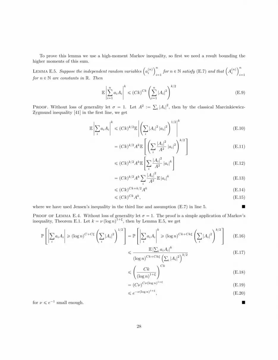
To prove this lemma we use a high-moment Markov inequality, so first we need a result bounding thehigher moments of this sum.

Lemma E.5. Suppose the independent random variables´

apnqi

¯n

i“1for n P N satisfy (E.7) and that

´

Apnqi

¯n

i“1for n P N are constants in R. Then

E

∣∣∣∣∣ nÿi“1

aiAi

∣∣∣∣∣k

ď pCkqCk

˜

nÿ

i“1

|Ai|2¸k2

(E.9)

Proof. Without loss of generality let σ “ 1. Let A2 :“ř

i |Ai|2, then by the classical Marcinkiewicz-

Zygmund inequality [41] in the first line, we get

E

∣∣∣∣∣ÿi

aiAi

∣∣∣∣∣k

ď pCkqk2E

∣∣∣∣∣∣˜

ÿ

i

|Ai|2 |ai|2¸12

∣∣∣∣∣∣k

(E.10)

“ pCkqk2AkE

»

–

˜

ÿ

i

|Ai|2

A2|ai|2

¸k2fi

fl (E.11)

ď pCkqk2AkE

«

ÿ

i

|Ai|2

A2|ai|k

ff

(E.12)

“ pCkqk2Akÿ

i

|Ai|2

A2E |ai|k (E.13)

ď pCkqCk`k2Ak (E.14)

ď pCkqCkAk, (E.15)

where we have used Jensen’s inequality in the third line and assumption (E.7) in line 5.

Proof of Lemma E.4. Without loss of generality let σ “ 1. The proof is a simple application of Markov’sinequality, Theorem E.1. Let k “ ν plog nq

1`ξ, then by Lemma E.5, we get

P

»

–

∣∣∣∣∣ÿi

aiAi

∣∣∣∣∣ ě plog nqC`Cξ

˜

ÿ

i

|Ai|2¸12

fi

fl “ P

»

–

∣∣∣∣∣ÿi

aiAi

∣∣∣∣∣k

ě plog nqCk`Ckξ

˜

ÿ

i

|Ai|2¸k2

fi

fl (E.16)

ďE |

ř

i aiAi|k

plog nqCk`Ckξ

´

ř

i |Ai|2¯k2

(E.17)

ď

˜

Ck

plog nq1`ξ

¸Ck

(E.18)

“ pCνqCνplognq1`ξ (E.19)

ď e´νplognq1`ξ

, (E.20)

for ν ď e´1 small enough.

28

References

[1] Benjamin Allen, Jeff Gore, and Martin A Nowak. Spatial dilemmas of diffusible public goods. Elife,2:e01169, 2013.

[2] Tibor Antal, Sidney Redner, and Vishal Sood. Evolutionary dynamics on degree-heterogeneous graphs.Phys. Rev. Lett., 96:188104, 2006.

[3] Albert-Laszlo Barabasi and Reka Albert. Emergence of scaling in random networks. Science.,286(5439):509–512, 1999.

[4] Valmir C. Barbosa, Raul Donangelo, and Sergio R. Souza. Early appraisal of the fixation probabilityin directed networks. Phys. Rev. E, 82:046114, 2010.

[5] Alain Barrat and Martin Weigt. On the properties of small-world network models. Eur. Phys. J. B,13(3):547–560, 2000.

[6] NH Barton. The probability of fixation of a favoured allele in a subdivided population. Genet. Res.,pages 149–157, 1993.

[7] Alexei Borodin and Vadim Gorin. Lectures on integrable probability. pre-print, 2012.

[8] Mark Broom and Jan Rychtar. An analysis of the fixation probability of a mutant on special classes ofnon-directed graphs. Proc. R. Soc. A Math. Phys. Eng. Sci., 464(2098):2609–2627, 2008.

[9] Mark Broom and Jan Rychtar. Game-theoretical models in biology. Chapman & Hall/CRC mathematicaland computational biology series. Chapman and Hall/CRC Press, Taylor and Francis Group, BocaRaton, FL, 2013.

[10] Mark Broom, Jan Rychtar, and B Stadler. Evolutionary dynamics on small-order graphs. J. Interdiscip.Math., 12:129–140, 2009.

[11] Yu-Ting Chen. Sharp benefit-to-cost rules for the evolution of cooperation on regular graphs. Ann.Appl. Probab., 23(2):637–664, 2013.

[12] Fan Rong King Chung and Linyuan Lu. Complex graphs and networks, volume no. 107 of CBMS regionalconference series in mathematics ;. American Mathematical Society, Providence, RI, 2006.

[13] Percy Deift. Universality for mathematical and physical systems. Proc. Int. Congr. Math., 2006.

[14] Josep Dıaz, Leslie Ann Goldberg, George B. Mertzios, David Richerby, Maria Serna, J., and Paul G.Spirakis. On the fixation probability of superstars. Proc. R. Soc. A Math. Phys. Eng. Sci., 469:20130193,2013.

[15] Richard Durrett and Simon Levin. The Importance of Being Discrete (and Spatial). Theor. Popul.Biol., 46:363–394, 1994.

[16] Richard Durrett and Simon A Levin. Stochastic spatial models: a user’s guide to ecological applications.Philos. Trans. R. Soc. London. Ser. B Biol. Sci., 343(1305):329–350, 1994.

[17] Laszlo Erdos and Horng-Tzer Yau. Universality of local spectral statistics of random matrices. Bull.Am. Math. Soc., 49(3):377–414, 2012.

29

[18] Paul Erdos and Alfred Renyi. On the evolution of random graphs. Publ. Math. Inst. Hungarian Acad.Sci., 5, 1960.

[19] Marcus Frean, Paul B Rainey, and Arne Traulsen. The effect of population structure on the rate ofevolution. Proc. R. Soc. B Biol. Sci., 280(1762):20130211, 2013.

[20] Christoforos Hadjichrysanthou, Mark Broom, and Istvan Z Kiss. Approximating evolutionary dynamicson networks using a Neighbourhood Configuration model. J. Theor. Biol., 312:13–21, 2012.

[21] Michael P Hassell, Hugh N Comins, and Robert M May. Species coexistence and self-organizing spatialdynamics. Nature, 370:290–292, 1994.

[22] Jaroslav Ispolatov and Michael Doebeli. Diversification along environmental gradients in spatiallystructured populations. Evol. Ecol. Res., 11:295–304, 2009.

[23] Alastair Jamieson-Lane and Christoph Hauert. Fixation probabilities on superstars, revisited and re-vised. pre-print, 2013.

[24] Karin Johst, Michael Doebeli, and Roland Brandl. Evolution of complex dynamics in spatially structuredpopulations. Proc. R. Soc. B Biol. Sci., 266(1424):1147–1154, 1999.

[25] Benjamin Kerr, Margaret a Riley, Marcus W Feldman, and Brendan J M Bohannan. Local dispersalpromotes biodiversity in a real-life game of rock-paper-scissors. Nature, 418(6894):171–4, July 2002.

[26] Mickael Le Gac and Michael Doebeli. Environmental viscosity does not affect the evolution of cooper-ation during experimental evolution of colicigenic bacteria. Evolution, 64(2):522–33, 2010.

[27] Michel Ledoux. The concentration of measure phenomenon, volume v. 89 of Mathematical surveys andmonographs,. American Mathematical Society, Providence, R.I., 2001.

[28] Simon A Levin. Population dynamic models in heterogeneous environments. Annu. Rev. Ecol. Syst.,7(1):287–310, 1976.

[29] Simon A Levin and Robert T Paine. Disturbance, patch formation, and community structure. Proc.Natl. Acad. Sci., 71(7):2744–2747, 1974.

[30] Erez Lieberman, Christoph Hauert, and Martin A Nowak. Evolutionary dynamics on graphs. Nature,(JANUARY):312–316, 2005.

[31] Takeo Maruyama. A Markov process of gene frequency change in a geographically structured population.Genetics, 76(2):367–377, 1974.

[32] Takeo Maruyama. A simple proof that certain quantities are independent of the geographical structureof population. Theor. Popul. Biol., 5(2):148–154, 1974.

[33] Patrick Alfred Pierce Moran. The statistical processes of evolutionary theory. Oxford University Press,Oxford, England, 1962.

[34] Mayuko Nakamaru and Simon A Levin. Spread of two linked social norms on complex interactionnetworks. J. Theor. Biol., 230(1):57–64, 2004.

[35] Martin A Nowak. Evolutionary dynamics : exploring the equations of life. Belknap Press of HarvardUniversity Press, Cambridge, Massachusetts, 2006.

30

[36] Martin A Nowak, Franziska Michor, and Yoh Iwasa. The linear process of somatic evolution. Proc.Natl. Acad. Sci. U. S. A., 100(25):14966–14969, 2003.

[37] Hisashi Ohtsuki, Christoph Hauert, Erez Lieberman, and Martin A Nowak. A simple rule for theevolution of cooperation on graphs and social networks. Nature, 441:502–505, 2006.

[38] Z Patwa and Lindi M Wahl. The fixation probability of beneficial mutations. J. R. Soc. Interface,5(28):1279–1289, 2008.

[39] Paul B Rainey and Katrina Rainey. Evolution of cooperation and conflict in experimental bacterialpopulations. Nature, 425:72–74, 2003.

[40] B Sinervo and C M Lively. The rock-paper-scissors game and the evolution of alternative male strategies.Nature, 380:240 – 243, 1996.

[41] Daniel W Stroock. Probability theory : an analytic view. Cambridge University Press, Cambridge, UK,2nd edition, 2011.

[42] Duncan J Watts and Steven H Strogatz. Collective dynamics of ’small-world’ networks. Nature, 393:440–442, 1998.

[43] MC Whitlock. Fixation probability and time in subdivided populations. Genetics, 779(June):767–779,2003.

31