Efficient Estimation of Reflectance Parameters from

Imaging Spectroscopy

Lin Gu, Student Member, IEEE, Antonio Robles-Kelly, Senior Member, IEEE,

and Jun Zhou, Senior Member, IEEE

Abstract

In this paper, we address the problem of efficiently recovering the reflectance parameters from a single

multispectral or hyperspectral image. To do so, we propose a Shapelet Based Estimator (SBE) which employs

shapelets to recover the shading in the image. The optimisation setting presented here is based upon a three-

step process. The first of these concerns the recovery of the surface reflectance and the specular coefficients via

a constrained optimisation approach. Secondly, we update the illuminant power spectrum using a simple least-

squares formulation. Finally, the shading is computed directly once the updated illuminant power spectrum is at

hand. This yields a computationally efficient method which achieves speed-ups of nearly an order of magnitude

over its closest alternative without compromising performance. We provide results on illuminant power spectrum

computation, shading recovery, skin recognition and replacement of the scene illuminant and object reflectance in

real-world images.

Index Terms

Keywords: Multispectral and hyperspectral imaging, Scene analysis, Inverse methods for imaging spectroscopy

I. INTRODUCTION

The recovery of shape and photometric invariants through imaging spectroscopy can provide a means

for identification and recognition purposes. Further, photometric invariants can be used in combination

with the object shape and light power spectrum for advanced applications in photowork, visualisation,

Copyright (c) 2013 IEEE. Personal use of this material is permitted. However, permission to use this material for any other purposes mustbe obtained from the IEEE by sending a request to pubs-permissions@ieee.org.

L. Gu is with the Research School of Engineering at the Australian National University, Canberra, ACT 2601, Australia.

A. Robles-Kelly is with the National ICT Australia (NICTA) and the College of Engineering and Computer Science at the AustralianNational University, Canberra, ACT 2601, Australia.

J. Zhou is with the School of Information and Communication Technology at Griffith University, Nathan, QLD 4111, Australia.

NICTA is funded by the Australian Government as represented by the Department of Broadband, Communications and the Digital Economyand the Australian Research Council through the ICT Centre of Excellence program.

1

Fig. 1. Initial (left-hand panel) and final (right-hand panel) pseudocolour images when the skin reflectance of the subject is substituted byan alternative. The left-hand panel shows the pseudocolour image of a portrait taken using a hyperspectral camera. The skin reflectance ofthe subject is plotted on the top middle panel whereas the one used as an alternative is shown in the bottom middle plot. The right-handpanel, has been recovered by effecting skin recognition so as to locate those pixels whose spectra are to be replaced. The image irradiancehas then been recomputed using the photometric parameters recovered by our method and the alternative reflectance. Note that a similarsequence of events would apply to the replacement of the illuminant in the scene, where the power spectrum of the light has to be recoveredand substituted.

creation and manipulation of digital media [1]. This is illustrated in Figure 1, where we show the result

of substituting the skin reflectance in a portrait.

Despite its prospective applications, the recovery of photometric invariants from imaging spectroscopy

is not a straightforward task. This is since every scene comprises a rich tapestry of light sources, material

reflectance and lighting effects due to object curvature and shadows. Moreover, trichromatic (i.e. RGB)

technology does have limits in its scene analysis capabilities. For example, a camera with a RGB sensor

is prone to metamerism and, therefore, can not deliver photometric invariants characteristic to a material

independent of the lighting or shape.

Along these lines, in computer vision and image processing, most of the efforts in the literature have

been devoted to modelling the effects encountered on shiny or rough surfaces. For shiny surfaces, specular

spikes and lobes have to be modelled. There have been several attempts to remove specularities from

images of non-Lambertian objects, i.e. the objects whose surface brightness is the same regardless of

the observer angle of view. For instance Brelstaff and Blake [2] used a simple thresholding strategy to

identify specularities on moving curved objects. Other lines of research remove specularities by either

using additional hardware [3], imposing constrains on the input images [4], requiring color segmentation

[5] as postprocessing steps, or using reflectance models to account for the distribution of image brightness

[6].

2

Moreover, the methods above often rely on the use of the closed form of the Bidirectional Reflectance

Distribution Function (BRDF). As a result, they lack the generality required to process real-world imagery

in an unsupervised or automatic way. Moreover, for rough surfaces, the main bulk of research focuses on

the loss of contrast at the object limbs and an apparent flattening of perceived relief [7], [8], [9], [10].

Hence, the accurate modelling of object limb brightening for rough surface reflectance has proved to be

extremely elusive, and is still an active area of research in applied optics.

The applicability of existing methods to imaging spectroscopy is further limited by the difficulty in

extending these methods to images comprised of tens or even hundreds of bands. This is mainly due

to the complexity regarding a closed form solution for the high-dimensional image data involved, but is

also related to the fact that the BRDF parameters become wavelength dependent and, hence, are often

intractable. Moreover, any pre/postprocessing and local operations on the reflectance must be exercised

with caution and in relation to neighbouring spectral bands so as to prevent spectral signature variation.

To solve these problems, Healey and his colleagues [11], [12] studied photometric invariance in hyper-

spectral aerial imagery for material classification and mapping as related to photometric artifacts induced

by atmospheric effects and changing solar illuminations. In [13], a method is presented for hyperspectral

edge detection. The method is robust to photometric effects, such as shadows and specularities. In [14],

a photometrically invariant approach was proposed based on the derivative analysis of the spectra. This

local analysis of the spectra was shown to be intrinsic to the surface reflectance. Yet, the analysis in [14]

was derived from the Lambertian reflection model and, hence, is not applicable to specular reflections.

Recently, Huynh and Robles-Kelly [15] proposed a method based upon an the dichromatic model [16]

aimed at imaging spectroscopy. Despite effective, the method can be computationally demanding since it

relies upon a dual-step gradient descent optimisation scheme governed by a regularised cost function.

Estimation of reflectance parameters is also closely related to the problem of recovering the shape of an

object from its shading information. The classic approaches to shape from shading developed by Ikeuchi

and Horn [17], and by Horn and Brooks [18], hinge on the compliance with the image irradiance equation

and local surface smoothness. Zheng and Chellappa [19] proposed a gradient consistency constraint that

penalises differences between the image intensity gradient and the surface gradient for the recovered

surface. Worthington and Hancock [20] impose the Lambertian radiance constraint in a hard manner.

Dupuis and Oliensis [21] provided a means of recovering probably correct solutions with respect to

the image irradiance equation. Prados and Faugeras [22] have presented a shape from shading approach

3

applicable to the case where the light source and viewing directions are no longer co-incident. Kimmel

and Bruckstein have used the apparatus of level sets methods to recover solutions to the Eikonal equation

[23].

Here, we present a method based upon shapelets [24] which recovers the reflection parameters, i.e.

shading, specularities, light spectral power and surface reflectance, from the image radiance. Note that

the capacity to recover the power spectrum of the illuminant, reflectance and shading is reminiscent

of the method in [15]. Despite its effectiveness, the work presented in [15] can be computationally

costly. Moreover, the method presented here permits the use of robust statistics [25] and makes use of an

alternative formulation which yields a different optimisation scheme. This optimisation strategy can be

further simplified to yield improvements in computational efficiency of an order of magnitude over the

method in [15].

The paper is organised as follows. We commence by introducing the motivation to the method presented

in this paper and ellaborating upon the relevant background in the next section. In Section II, we present the

dichromatic reflection model and provide a link between the work in [16]. We discuss the implementation

issues of our method, its initialisation and the extensions to trichromatic imagery in Section III. In Section

IV, we present results for our method and, finally, we conclude on the developments presented here in

Section V.

II. ESTIMATING THE REFLECTION PARAMETERS

To recover the reflection parameters, we employ the Dichromatic model in [16]. This model has long

been used in physics-based vision for characterising specular reflections on non-Lambertian surfaces. The

model states that the radiance for a pixel in the image can be expressed as follows

I(λi, u) = g(u)L(λi)S(λi, u) + k(u)L(λi) (1)

where L(λi) is the light source spectral component as a function of the ith band with wavelength λi,

S(λi, u) is the surface reflectance and g(u) and k(u) are the shading factor and specular coefficient at

the pixel location u. These are wavelength-independent and are governed by the illumination and surface

geometries.

In Equation 1, the first term on the right-hand side corresponds to the diffuse reflection, whereas the

second term accounts for the specularities. We can give an intuitive interpretation to the model as follows.

4

At specular pixels, i.e. where the shading factor g(u) is negligible, the surface acts as a mirror, where

the radiance becomes proportional to the illuminant power spectrum L(λi). On the other hand, if the

radiance is diffuse, i.e. k(u) is close to zero, then the surface appears shaded and the reflectance becomes

a multiplicative term on the illuminant to determine the radiance. This can be easily verified by writing

I(λi, u)

L(λi)= r(λi, u) + k(u) (2)

where r(λi, u) = g(u)S(λi, u)

is devoid of the illuminant spectrum L(λi) and proportional to the reflectance through the shading factor

g(u).

Note that, following the model in Equation 2, it would be straightforward to recover the specular

coefficient k(u) if the other parameters were at hand. Similarly, by assuming the illuminant spectrum

and the specular coefficient k(u) are available, one could normalise the irradiance and recover the term

r(λi, u). This suggests an iterative process involving the recovery of the shading factor, estimation of the

specular coefficient k(u) and reflectance so as to achieve a solution for the illuminant power spectrum

L(λi).

For now, we will assume initial estimates for the reflection model parameters are at hand. We will

discuss the computation of the initial parameter values in Section III. With these initial values, we

can estimate the photometric parameters via a three-step iterative process. Firstly, the shading factor is

computed. Secondly, the surface reflectance and the specular coefficients are computed using a constrained

optimisation approach. Finally, the illuminant power spectrum can be recovered from the above parameters

that have been recovered. These three interleaved steps are applied until convergence is reached.

A. Recovery of the Shading Factor

As mentioned above, we employ shapelets so as to recover the shading factor in Equation 2. The idea

underpinning our method is that the shading factor g(u) can be viewed as that governing the diffuse

reflection from the surface. As a result, we can use Lambert’s Law [26] and setg(u) = cos(α, u) where

α is the angle between the light source direction and the surface normal. This angle can be computed

via the inner product of the surface normal and the illuminant direction in a straightforward manner from

the surface normal if the light source direction is known. Later on in this section, we discuss how the

requirement pertaining the light source direction to be known can be removed. For now, we assume the

5

light source direction is available and focus on the computation of the shading factor.

If the 3D representation of the object surface is at hand, the shading factor computation becomes the

matter of a simple inner product. Unfortunately, the recovery of the 3D representation of the surface is a

non-trivial task. In [24], shapelets are used as a complete orthonormal set of basis functions so that the 3D

representation of the surface can be easily recovered despite the effects of noise corruption. Shapelets are

a set of basis functions with finite support used in image analysis in a manner akin to Fourier or wavelet

synthesis. These basis functions or shapelets can be Hermite polynomials [27] or an over complete basis

such as that in [28]. Since a complete treatise on shapelets is beyond the scope of this paper, we would

like to refer the interested reader to the book of Mallat [29] or the paper by Refregier [27].

In [24], the recovery of the 3D surface is effected by correlating the slant and tilt of the field of surface

normals with those of the shapelets. The main contribution in [24], hinges upon the recovery of the 3D

shape from a sum of correlations between the surface gradients and the basis functions, i.e. the shapelets.

In practice, the correlation can be computed via a convolution, whereas the tilt of the surface normal can

be recovered using the direction of the image gradient on the image plane [24]. Here, we follow [24] and

depart from a shapelet based upon the tangent function. As shown in [24], the 3D surface reconstruction

H is given by the sum over the scales q for the shapelets tan(sq), where sq is the slant of the shapelet

normals. Thus, the reconstruction is given by

H =∑q

| tan(α)| ∗ | tan(sq)| · | cos(τf ) ∗ cos(τq) + sin(τf ) ∗ sin(τq)| =∑q

| tan(α)| ∗ | tan(sq)| ·Cτq (3)

where τq and τf correspond to the tilt of the normals for both, the shapelet and the object under study,

respectively. In Equation 3, α is the angle between the surface normal and the light direction and ∗ denotes

convolution.

Unfortunately, the angle α remains a variable to be estimated and, therefore, the equation above cannot

be used directly. Nonetheless, making use of Equations 2,we can derive the following relation

1

r(λi, u)− r(λj, u)= sec(α, u)

1

(S(λi, u)− S(λj, u))(4)

Note that tan(α), sec(α) and sec(α)− 1 share an akin monotonically increasing behavior in [0, π2]. In

Figure 2, we show a sample shape and the corresponding 3D reconstructions recovered using tan(α) and

sec(α) − 1. Note that the reconstructions yielded by both functions are in close accordance with each

other and the ground truth. As a result, we can use sec(α)−1 as an alternative to tan(α) and approximate

6

the shapelet reconstruction for each band by

Hλi ≈∑q

Rλi ∗ | tan(sq)| · Cτq (5)

where Rλi is a matrix whose entry indexed u is given by∣∣∣∣S(λi,u)−S(λj ,u)r(λi,u)−r(λj ,u) − 1

∣∣∣∣.

Fig. 2. Left-hand panel: 3D Block ground truth shape; Middle panel: shapelet reconstruction yielded using tanα; Right-hand panel:reconstruction obtained using sec(α)− 1.

Recall that tan(sq) and Cτq are known and can be readily computed from the shapelet basis functions and

the image gradients. Theoretically, any arbitrarily chosen reference band λj can be used for the difference

above. Nonetheless, r(λj, u) and S(λj, u) may deviate from the ideal case as modelled by Equation 2 due

to measurement noise. This is compounded by the fact that, in practice, the surface reconstruction can be

recovered for each band in the image.

To tackle both the ambiguity of the surface reconstruction to band index and noise corruption, we assume

that the measurement errors are independent and identically distributed random variables governed by a

Gaussian distributions with zero mean. It can be shown that under this assumption, the variance of the

estimate can be much reduced through averaging [25]. Thus, instead of an arbitrary reference band, we

use the mean of r(·, u) and S(·, u) given by

r∗u =1

N

N∑j=1

r(λj, u) S∗u =1

N

N∑j=1

S(λj, u) (6)

where N is the total number of bands in the image. For the computation of the matrix Rλi in Equation

5, we employ the resulting r∗u and S∗u from the equations above as an alternative to the quantities r(λj, u)

and S(λj, u) corresponding to an arbitrary band indexed j.

Following a similar rationale regarding the surface reconstruction estimates for each band, we make

7

use of the average

H∗ =1

N

N∑j=1

Hλj (7)

as an alternative to H in Equation 3. With the surface reconstruction H∗ at hand, the quantity cos(α, u)

at each pixel u can be computed making use of the light source direction and the surface normal field

over H∗.

B. Computation of the Reflectance and Specular Coefficient

We now make use of the illuminant and the shading factor to recover the the reflectance S(λi, u) and

the specular coefficient k(u). Since the cos(α, u) has been computed using shapelets as presented in the

previous section, we can recovery the surface reflectance using the following equation

S(λi, u)∗ =

1

cos(α, u)

(I(λi, u)

L(λi)− k(u)∗

)(8)

where k(u)∗ is the estimated specular coefficient given by

k(u)∗ = mink(u)≥0

{ N∑j=1

|I(λj, u)− L(λj)(g(u)S(λj, u)

∗ − k(u))|2}

The expressions above are consistent with both, the Dichromatic model presented earlier and the notion

that the specular coefficient should be a positive real-valued quantity. In practice, the recovery of the

specular coefficient can be effected making use of a constrained least squares approach. In Section III,

we comment further on our implementation.

C. Illuminant Power Spectrum Computation

To estimate the illumination, we note that the light power spectrum L(λi) in Equation 1 does not depend

upon the pixel-wise variable u. Although the radiance sensed by the camera can be influenced by shadows

and other changes such as the specular spike brightness, the spectral power distribution of the illuminant

does not change. This indicates that the illuminant is a global photometric variable throughout the image.

This observation is important since we can recover its spectrum by minimising the cost function given by

L(λi)∗ = arg min

L(λi)

{∑u∈I

| I(λi, u)−(cos(α, u)S(λi, u)

∗ + k(u)∗)L(λi) |2

}(9)

8

where I is the set of all pixels in the imagery. Since the only unknown in the cost function above is the

light spectrum L(·), the above minimisation becomes a least squares one whose solution is unique and

computationally efficient.

1) Simplification of the Model: To simplify the method above, we note that, in real-world imagery,

a number of pixels often show a large specular component. This is particularly evident at the specular

spikes in the image. For these pixels, the specular coefficient is, in practice, much larger than the shading

factor, i.e. k(u) � g(u). This implies that, for those pixels with a large specular component, we have

I(λi, u) ≈ k(u)L(λi) where we have substituted the shorthand g(u) ≈ 0 into Equation 1.

We note that, whereas accordance to the dirchromatic plane implies a diffuse reflection, deviation from

the dichromatic plane indicates large specular coefficients. As a result, we can ignore the diffuse term

g(u)S(λi, u) in Equation 1 for those pixels comprising the set P of K-most specular patches and recover

the illuminant power spectrum by minimising the expression

L(λi)∗ = arg min

L(λi)

{∑u∈P

| I(λi, u)− k(u)∗L(λi) |2}

(10)

as an alternative to Equation 9.

2) Application of Robust Statistics: Note that, in practice, imaging spectroscopy is not devoid of noise

corruption. Further, for our illumination recovery step, we use a least-squares minimisation scheme. This

least-squares approach, despite effective, can be sensitive to outliers.

To tackle this problem, we can employ robust statistics as an alternative to least-squares. Robust

statistics provide a means to noise corruption by introducing an estimator which is robust to outliers.

There are a number of robust estimators that can be used, such as maximum likelihood (M-estimators),

linear combination of order statistics (L-estimators), rank transformation (R-estimators) and repeated M-

estimators (RM-estimators) [30], [25].

To apply these estimators to our illuminant recovery step, we assume that the image radiance for those

pixel-sites u ∈ P can be modeled as a linear combination of the true specularities k(u)L(λi) and a noise

component η(u). The image radiance, i.e. the observable, becomes I(λi, u) = k(u)L(λi) + η(u). With

these ingredients, we can set an error penalty function g(·) so as to provide an alternative to Equation 10

as follows

L(λi)∗ = arg min

L(λi)

{∑u∈P

g(I(λi, u)− k(u)∗L(λ)}

= arg minL(λi)

{g(η(u)

)}(11)

9

Fig. 3. Left-hand panel: The reflection geometry making use of an arbitrary reference e; Middle panel: Shape-from-shading treatment wherethe viewpoint corresponds to the z-axis of the reference; Right-hand panel: The reflection geometry when the reference is given such thatlight source direction becomes ~L ≡ [0, 0, 1]T .

D. On the Light Source Direction

Recall that, in the previous sections, we assumed that the light source direction ~L was known. In

practice, this may not be the case. To relax the restriction, we note that, according to Lambert’s Law, for

the pixel indexed u corresponding to the point p on H∗ illuminated from the direction ~L, the shading

factor g(u) is given by (~Np · ~L), where Np is the normal to the surface H∗ at p.

By substituting the shorthand g(u) = (~Np ·~L) into Equation 1 we getI(λi, u) = L(λ)((~Np ·~L)S(λi, u)+

k(u)) where we have used notation consistent to that introduced in Section II-A.

To remove the restriction associated to a known illuminant direction, we make use of the fact that the

light direction in the scene can be measured relative to an arbitrary reference e = [ex, ey, ez]T . This is

illustrated in the left-hand panel of Figure 3. In the figure, we show the reference axis, the surface normal

and the viewer and light directions making use of a sample surface H∗. Here, we let the reference be

such that the light direction becomes ~L ≡ [0, 0, 1]T . That is, we set the reference of the surface H∗ such

that the estimated shading factor satisfies the relation g(u)∗ = cos(α, u) = (~Np · ~L)

This contrasts with shape-from-shading approaches [31], where the aim of computation is the surface

given by H∗. Here, H∗ is a means for the computation of g(u)∗ = cos(α, u) through the shorthand

g(u)∗ = (~Np · ~L). In shape-from-shading methods, the widely used reference is such that the camera axis,

i.e. the viewer direction, corresponds to the depth of the object. As exemplified in the right-hand panel

of Figure 3. In contrast, our choice of reference e has the effect of rotating the surface such that its depth

can no longer be measured with respect to the camera plane. As a result of the use of a reference in the

direction of the light source, the depth of the surface H∗ with respect to the viewer will be rotated in

the direction contrary to the viewer relative to the vector ~L. This rotation, however, does not affect the

10

angle α between the normal Np and the light source direction ~L. Since our aim of computation is not

the depth of the surface H∗ but the angle α, we set ~L ≡ [0, 0, 1]T in our computations without any loss

of generality and, hence, do not require the light source direction to be known a priori.

E. Extension to Trichromatic Imagery

Our method can also be applied to trichromatic images captured using RGB cameras. In trichromatic

imagery, each of the three colour channels has its own spectral sensitivity function, i.e. colour matching

function, Qc(·) for each of the bands λi, where c = {R,G,B}. As a result, the c-colour response at pixel

indexed u can be written in terms of the wavelength indexed radiance as follows

Ic(u) =N∑i=1

I(λi, u)Qc(λi) (12)

where we have written Ic to imply that the quantity above corresponds to the sum over the radiance

I(λi, u) at the pixel u as sensed by the camera with matching function Qc(·).

When we apply the equation above to the dichromatic model, we get

Ic(u) = g(u)

( N∑i=1

S(λi, u)Qc(λi)L(λi)

)+ k(u)

( N∑i=1

L(λi)Qc(λi)

)= g(u)Bc(u) + k(u)Lc (13)

where

Bc(u) =N∑i=1

S(λi, u)Qc(λi)L(λi) Lc =N∑i=1

L(λi)Qc(λi)

From Equation 13, we can conclude that our method can be applied to trichromatic imagery so as

to recover the parameters corresponding to the variables g(u), Bc(u), k(u) and Lc above. Nonetheless,

there are two important differences between these parameters and their wavelength-indexed counterparts.

Firstly, Lc does not account for the true illuminant power spectrum rather than its product with the

colour matching functions Qc(·). Secondly, the variable Bc(u) is a linear combination of the product of

wavelength-indexed reflectance and illuminant weighted by the colour matching function. As a result, to

further recover the analogue of the reflectance for trichromatic imagery, i.e. the albedo ρc(u), for the cth

colour channel at pixel indexed u, we use the following equation

ρc(u) =Bc(u)

Lc(14)

11

III. IMPLEMENTATION

Now we turn our attention to the implementation of our method. To this end, we present the corre-

sponding pseudocode in Algorithm 1. Note that, in the figure, we have altered slightly the computation

sequence with respect to that presented in Section II. The pseudocode takes at input the initial estimate

of the light power spectrum L(·)∗, the image I, the number of scales M used for the computation of the

shapelets and the threshold ε. It delivers at output the estimated illuminant power spectrum L∗new and the

values for the photometric parameters in the arrays G, K and S whose entry indexed u is given by g(u)∗,

k(u)∗ and S(·, u)∗, respectively.

The initial estimate of the illuminant power spectrum can be computed using a number of methods

elsewhere in the literature [15], [32], [33]. In our implementation, we select a set of “dichromatic” image

patches making use of the procedure in [15]. This is effected by subdividing the image into a lattice,

where the pixels in each rectangular patch in the lattice are then fitted to a two-dimensional hyperplane,

i.e. a dichromatic plane [16], spanned by the surface reflectance and the illuminant power spectrum. Here,

we regard a patch to be dichromatic if it contains a small percentage of pixels whose radiance is in close

accordance to their projection on the dichromatic plane. For a detailed description of the dichromatic

plane computation, we refer the reader to [16]. With these image patches at hand, we apply continuum

removal [34] so as to recover a pixel-wise estimate of the illuminant. The initial estimate of the illuminant

is given by the median over the continuum removed spectra for all the selected patches. This follows the

notion that the median is, effectively, a robust estimator [25].

Our pseudocode commences by computing the parameters sk and Cτk for the shapelets as described

in [24]. In Lines 3 and 4 we initialise S∗u and S(λj, u) such that, for the first iteration of the algorithm

S(λi, u)−S∗u ≡ 1. In Line 5, we initialise the specular coefficient k(u). To this end, we note that we can

always bound r(λi, u) to be between 0 and 1. We can give a physical interpretation to this assumption.

The bounded nature of r(λi, u) reflects the notion that the radiant power of light per unit of surface area,

as sensed by the camera, can always be scaled so its maximum value is unity. This, together with the

fact that, from Equation 2, the specular coefficient k(u) is an additive constant to r(λi, u), we initialise,

in Line 5, k(u) by setting it to the minimum value of the reflectance over the wavelength domain, i.e.

k(u)∗ = mini

{I(λi, u)

L(λi)

}

12

1: Input: L(·)∗, I, M and ε2: Compute sk and Cτk for k = 1, 2, . . . ,M3: Set S∗u ≡ 0 ∀ u ∈ I4: Set S(λj, u) ≡ 1 ∀ u ∈ I and k = 1, 2, . . . ,M

5: Set k(u)∗ = mini

{I(λi,u)L(λi)

}6: For u ∈ I7: r∗u =

1N

∑Nj=1

I(λj ,u)

L(λj)− k(u)∗

8: Rλi(u) =

∣∣∣∣ S(λi,u)−S∗u

I(λi,u)

L(λi)−k(u)∗−r∗u

∣∣∣∣9: For i = 1, 2, . . . , N

10: Hλi =∑M

k=1 R(λi) ∗ | tan(sk)| · Cτk11: Compute H∗ = 1

N

∑Nj=1Hλj

12: For u ∈ I13: g(u)∗ = (∇H∗|u, [0, 0, 1]T )14: For i = 1, 2, . . . , N

15: S(λi, u)∗ = 1

g(u)∗

(I(λi,u)L(λi)

− k(u)∗)

16: Set Lnew(λi) via Section II-C17: Compute S∗u = 1

N

∑Nj=1 S(λj, u) ∀ u ∈ I

18: For u ∈ I

19: Compute k(u)∗ = mink(u)≥0

{∑Nj=1 |I(λj, u)

−Lnew(λj)(g(u)∗S(λj, u)

∗ − k(u))|2}

20: If |L(·)∗ − Lnew| ≤ ε then21: Return L∗new, G, K and S22: Else23: L(·)∗ ← Lnew24: Go to Line 6

Algorithm 1: Pseudocode for our method

The initialisation of these parameters permits the computation of Rλi(u) in Line 8. In Lines 7 and 17,

we compute r∗u and S∗u as presented in Section II-A. In Algorithm 1, we have used the fact that, making

use of H∗, we can express the normal Np = ∇H∗|u∼p, where the expression u ∼ p implies that the pixel

indexed u ∈ I corresponds to the point p ∈ H∗. Note that the pseudocode is such that, if the change

in the estimated illuminant power spectrum is less or equal to the threshold ε, it returns the photometric

parameters. Otherwise it goes to Line 6 so as to iterate accordingly. The optimisation in Line 19, which

yields the updated specular coefficient has been effected using a constrained least squares based upon a

Newton algorithm [35].

13

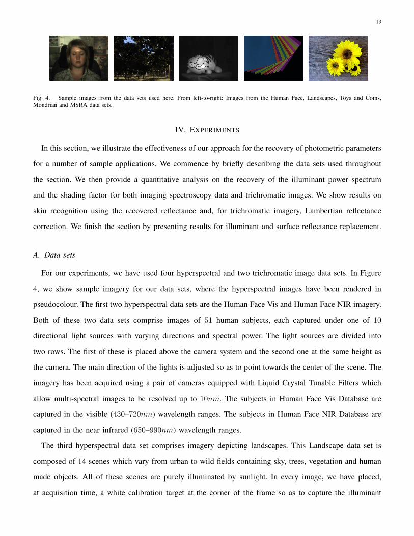
Fig. 4. Sample images from the data sets used here. From left-to-right: Images from the Human Face, Landscapes, Toys and Coins,Mondrian and MSRA data sets.

IV. EXPERIMENTS

In this section, we illustrate the effectiveness of our approach for the recovery of photometric parameters

for a number of sample applications. We commence by briefly describing the data sets used throughout

the section. We then provide a quantitative analysis on the recovery of the illuminant power spectrum

and the shading factor for both imaging spectroscopy data and trichromatic images. We show results on

skin recognition using the recovered reflectance and, for trichromatic imagery, Lambertian reflectance

correction. We finish the section by presenting results for illuminant and surface reflectance replacement.

A. Data sets

For our experiments, we have used four hyperspectral and two trichromatic image data sets. In Figure

4, we show sample imagery for our data sets, where the hyperspectral images have been rendered in

pseudocolour. The first two hyperspectral data sets are the Human Face Vis and Human Face NIR imagery.

Both of these two data sets comprise images of 51 human subjects, each captured under one of 10

directional light sources with varying directions and spectral power. The light sources are divided into

two rows. The first of these is placed above the camera system and the second one at the same height as

the camera. The main direction of the lights is adjusted so as to point towards the center of the scene. The

imagery has been acquired using a pair of cameras equipped with Liquid Crystal Tunable Filters which

allow multi-spectral images to be resolved up to 10nm. The subjects in Human Face Vis Database are

captured in the visible (430–720nm) wavelength ranges. The subjects in Human Face NIR Database are

captured in the near infrared (650–990nm) wavelength ranges.

The third hyperspectral data set comprises imagery depicting landscapes. This Landscape data set is

composed of 14 scenes which vary from urban to wild fields containing sky, trees, vegetation and human

made objects. All of these scenes are purely illuminated by sunlight. In every image, we have placed,

at acquisition time, a white calibration target at the corner of the frame so as to capture the illuminant

14

power spectrum ground truth. It is worth noting that, so as to avoid any unfair advantage of our method

or the alternatives when processing the Landscape imagery, this calibration target has been cropped from

the imagery at processing time.

The fourth hyperspectral data set comprises imagery obtained using a camera equipped with an Acousto-

Optic Tunable Filter. This filter allows tuning to be effected at steps of 1nm. The data set comprises images

corresponding to five categories of toys and a set of s. Each toy sample was acquired over ten views by

rotating the object in increments of 10 ◦ about its vertical axis whereas the imagery was captured only in

two different views, heads and tails. In our data set, there are in total of 62 toys and 32 coins, which, over

multiple viewpoints yielded 684 hyperspectral images. Each image is comprised of 51 bands for those

wavelengths ranging from 550 to 1000 nm over 9nm steps. For purposes of photometric calibration, we

have also captured an image of a white Spectralon calibration target so as to recover the power spectrum

of the illuminant across the scene.

As mentioned above, the other two data sets are trichromatic. The first of these is the Mondrian image

data set described in [36] 1. This is a colour constancy data set containing 743 images of objects illuminated

under 11 different illuminants whose ground truth is available. Lastly, we have used the MSRA salient

object image data set [37] for our Lambertian reflectance correction results 2.

B. Illuminant Power Spectrum Recovery

We first turn our attention to the recovery of the illuminant power spectrum. To this end, we have

used Human Face Vis, Human Face NIR, Coins and Toys, Landscape and the Mondrian data sets. To

compute the accuracy of the recovered illuminant with respect to the ground truth, we have employed

two similarity measures. The first of these is the Spectral Information Divergence (SID) [38], which is

an information theoretic measure which assesses similarity making use of the probabilistic discrepancy

between the spectra under consideration. The SID is widely used in processing hyperspectral image data.

Se have also employed the Euclidean angle, which has also been widely used in the literature and is given

by

dangle = cos−1( ∑N

k=1 L(λk)Lgt(λk)√(∑Nk=1 L(λk)

2)√(∑N

k=1 Lgt(λk)2)) (15)

Where L(λi) is the estimated illumination and Lgt(λi) is the ground truth illuminant.

1The data set is accessible at http://www2.cs.sfu.ca/~colour/data/2The imagery can be downloaded from http://research.microsoft.com/en-us/um/people/jiansun/salientobject/salient object.htm

15

Tukey Bi-weight function Andrews M-estimator

g(η(u)

)=

{1−(1−η(u)2)3

6if η(u) ≤ κ

16

Otherwiseg(η(u)

)=

{1−cos(πη(u))

π2 if η(u) ≤ κ1π2 Otherwise

Cauchy regulariser Huber Kernel

g(η(u)

)= ln(1+η(u)2)

4g(η(u)

)=

{η(u)2 if η(u) ≤ κ

2κ|η(u)| − κ2 Otherwise

Fig. 5. Penalty functions g(η(u)

)for the robust regularisers used in our experiments.

Making use of the measures above, we present the illumiant estimation result yielded by our Shapelet

Based Estimator (SBE), its simplification as presented in Section II-C1 and its extension to robust statistics

given in Section II-C2. For the use of robust statistics, the regularisers used here are the Tukey bi-weight

function [30], the Andrews M-estimator [39], the Cauchy regulariser [25] and the Huber kernel [25]. These

are used as error penalty functions g(·) in Equation 11. In Figure 5, we show the formal expressions for

the penalty functions used in our experiments. Note that these act as robust regularisers assigning a large

penalty to those estimates far away from the sensed radiance and a non-linear penalty to those closer

to the image values I(λi, u). Note that, in the equations in Figure 5, we have used the variable κ as a

bandwidth parameter. In all our experiments, we have set κ to be the equivalent of 10% of the dynamic

range of the camera.

Also, recall that the initial estimate of the illuminant can influence the results yielded by our SBE

method. This is since, as discussed in Section III, our method requires initial estimates of the photometric

parameters. As a result, we have compared our use of the median for the dichromatic patches with the

results yielded by two alternative initialisation schemes. The first of these employs a uniform initialisation

of the illuminant power spectrum, this is L(λi) ≡ υ, where υ is the mean over the set of maximum

radiance values for each band in the image. The second scheme employs the maximal radiance in each

band for any of the pixels in the set of dichromatic patches. Thus, in the former case we set the global

maximum for each band as the initial illuminant estimation without using the homogeneous patches,

whereas for the latter scheme we employ an approximation of the light continuum [40].

In Table I, we show the illuminant recovery performance for the three methods using the three initialisa-

tion schemes mentioned earlier when processing the hyperspectral data sets and the Mondrian trichromatic

one. In the table, the best performance per dataset have been typeset bold. Also, note that we provide

error measurements for the near-infrared (NIR), i.e. 650nm − 990nm, and the visible (VIS) bands, i.e.

16

TABLE IAVERAGE PERFORMANCE, MEASURED USING THE EUCLIDEAN ANGLE, YIELDED BY OUR SBE ILLUMINANT RECOVERY METHOD AND

ITS SIMPLIFIED ANALOGUE PRESENTED IN SECTION II-C1 (SBE SIMPLIFIED) ON OUR HYPERSPECTRAL DATA SETS AND THEMONDRIAN IMAGERY.

Data set Initialisation Method SBE SBE (simplified)

Human Face Vis DatabaseLight continuum approx. 7.1123± 2.3802 4.8431± 4.2883

Global radiance max. 7.8727± 3.0814 4.8985± 4.3139Dichromatic patch median 6.5048± 1.9252 3.1547± 4.2929

Human Face NIR DatabaseLight continuum approx. 3.3550± 0.9547 2.5624± 1.2623

Global radiance max. 3.1537± 1.0777 2.5632± 1.1195Dichromatic patch median 3.0898± 1.0486 3.1291± 1.1475

Landscape DatabaseLight continuum approx. 19.0984± 8.6352 15.3212± 5.1458

Global radiance max. 19.5287± 10.9002 13.4850± 5.6958Dichromatic patch median 19.3174± 7.0929 11.2873± 5.9089

Toys and coinsLight continuum approx. 11.7577± 4.7089 9.3796± 10.4101

Global radiance max. 15.9850± 4.6914 9.8006± 10.6195Dichromatic patch median 12.0502± 4.1861 7.9062± 10.2213

Mondrian data setLight continuum approx. 22.4693± 10.7677 6.2118± 9.3858

Global radiance max. 16.0533± 10.6651 5.7872± 9.1088Dichromatic patch median 14.8967± 10.5720 5.7857± 9.1126

430nm− 720nm of the human subject data set. This is to provide a consistent wavelength range to that

used in NIR face identification systems [41] which employ NIR illumination as a means to recognition.

From Table I, we observe that, in general, the NIR bands for the human subjects allow more accurate

illuminant recovery than their visible counterparts. Further, the median of for the dichromatic patches

outperforms the alternative in initialisation schemes regardless for all the data sets except the NIR face

imagery.

Following the results in Table I, from now on, we compare the performance of our method and the

alternatives when the median for the dichromatic patches is used for initialisation purposes. For all our

experiments, we compare the results of our SBE method, its simplification presented in Section II-C1

(SBE Simplified) and the application of robust statistics as per Section II-C2 with a number of alterntives.

The first of these is the method in [15]. We have chosen this alternative since its based upon a structural

optimization approach which recovers the spectra of the illuminant, the surface reflectance and the shading

and specular factors based upon the dichromatic model. Thus, it shares the multi-spectral nature of our

method. The second alternative is given by the method in [16]. We also compare our method with the

White Patch [42], Grey-World [43] and a Grey Edge [44] methods presented. For Grey Edge method, we

only use the 1st order.

In order to provide a fair comparison between the methods under consideration, we employ the

17

methodology in [44]. The methodology in [44] employs the mean, median, trimean, the mean for the best

25% and the worst 25% so as to better summarise non-Gausian error distributions. This is particularly

important since, as we will see later on, the error measurements across our data sets are not always

normally distributed.

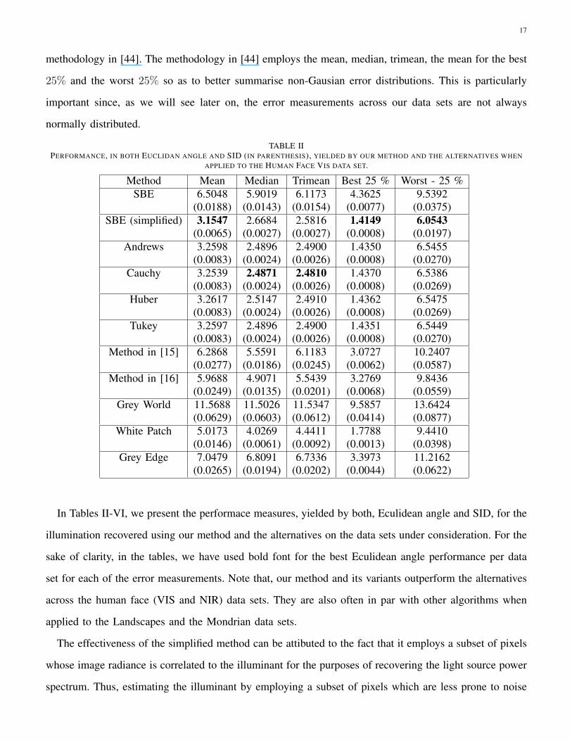
TABLE IIPERFORMANCE, IN BOTH EUCLIDAN ANGLE AND SID (IN PARENTHESIS), YIELDED BY OUR METHOD AND THE ALTERNATIVES WHEN

APPLIED TO THE HUMAN FACE VIS DATA SET.

Method Mean Median Trimean Best 25 % Worst - 25 %SBE 6.5048 5.9019 6.1173 4.3625 9.5392

(0.0188) (0.0143) (0.0154) (0.0077) (0.0375)SBE (simplified) 3.1547 2.6684 2.5816 1.4149 6.0543

(0.0065) (0.0027) (0.0027) (0.0008) (0.0197)Andrews 3.2598 2.4896 2.4900 1.4350 6.5455

(0.0083) (0.0024) (0.0026) (0.0008) (0.0270)Cauchy 3.2539 2.4871 2.4810 1.4370 6.5386

(0.0083) (0.0024) (0.0026) (0.0008) (0.0269)Huber 3.2617 2.5147 2.4910 1.4362 6.5475

(0.0083) (0.0024) (0.0026) (0.0008) (0.0269)Tukey 3.2597 2.4896 2.4900 1.4351 6.5449

(0.0083) (0.0024) (0.0026) (0.0008) (0.0270)Method in [15] 6.2868 5.5591 6.1183 3.0727 10.2407

(0.0277) (0.0186) (0.0245) (0.0062) (0.0587)Method in [16] 5.9688 4.9071 5.5439 3.2769 9.8436

(0.0249) (0.0135) (0.0201) (0.0068) (0.0559)Grey World 11.5688 11.5026 11.5347 9.5857 13.6424

(0.0629) (0.0603) (0.0612) (0.0414) (0.0877)White Patch 5.0173 4.0269 4.4411 1.7788 9.4410

(0.0146) (0.0061) (0.0092) (0.0013) (0.0398)Grey Edge 7.0479 6.8091 6.7336 3.3973 11.2162

(0.0265) (0.0194) (0.0202) (0.0044) (0.0622)

In Tables II-VI, we present the performace measures, yielded by both, Eculidean angle and SID, for the

illumination recovered using our method and the alternatives on the data sets under consideration. For the

sake of clarity, in the tables, we have used bold font for the best Eculidean angle performance per data

set for each of the error measurements. Note that, our method and its variants outperform the alternatives

across the human face (VIS and NIR) data sets. They are also often in par with other algorithms when

applied to the Landscapes and the Mondrian data sets.

The effectiveness of the simplified method can be attibuted to the fact that it employs a subset of pixels

whose image radiance is correlated to the illuminant for the purposes of recovering the light source power

spectrum. Thus, estimating the illuminant by employing a subset of pixels which are less prone to noise

18

TABLE IIIPERFORMANCE, IN BOTH EUCLIDAN ANGLE AND SID (IN PARENTHESIS), YIELDED BY OUR METHOD AND THE ALTERNATIVES WHEN

APPLIED TO THE HUMAN FACE NIR DATA SET.

Method Mean Median Trimean Best 25 % Worst - 25 %SBE 3.0898 2.9558 3.0289 2.0577 4.3342

(0.0039) (0.0032) (0.0035) (0.0016) (0.0072)SBE (simplified) 3.1291 1.8283 2.0243 0.7820 7.4315

(0.0089) (0.0012) (0.0021) (0.0002) (0.0301)Andrews 1.8867 1.6584 1.7640 0.7306 3.4097

(0.0021) (0.0009) (0.0016) (0.0002) (0.0058)Cauchy 1.8917 1.6775 1.7522 0.7291 3.3965

(0.0021) (0.0009) (0.0015) (0.0002) (0.0057)Huber 1.9102 1.6921 1.8114 0.7309 3.4188

(0.0022) (0.0011) (0.0017) (0.0002) (0.0058)Tukey 1.8866 1.6587 1.7645 0.7306 3.4091

(0.0021) (0.0009) (0.0016) (0.0002) (0.0058)Method in [15] 6.6822 6.3695 6.4752 3.7635 10.0058

(0.0207) (0.0160) (0.0178) (0.0053) (0.0425)Method in [16] 8.7401 9.2414 9.2357 4.9264 11.7016

(0.0352) (0.0353) (0.0356) (0.0106) (0.0595)Grey World 4.1531 3.6962 3.8341 2.8260 6.0701

(0.0078) (0.0053) (0.0059) (0.0031) (0.0161)White Patch 2.8205 2.2525 2.2746 0.9411 5.7469

(0.0054) (0.0024) (0.0026) (0.0003) (0.0164)Grey Edge 2.2417 2.0003 2.0951 1.5053 3.3173

(0.0022) (0.0017) (0.0018) (0.0009) (0.0043)

corruption. This is as the assumption of a large specular coefficient indirectly implies that the illuminant

is almost directly proportional to the image radiance for a pixel whose intensity is large and, hence, has

a high SNR with respect to noise and the strength of light impinging on the sensor. It is worth noting in

passing that this is somewhat akin to the white patch method. Nonetheless, our approach does not employ

the brightest pixel in the image, but rather the ones such that I(λi, u) ≈ k(u)L(λi).

Note that this simplification does not affect the recovery of the reflectance, shading factor or specular

coefficient. Also, note that the robust statistics application improves, in general, the results in the median

and the mean of best 25%. Further, the robust statistics do improve the results for the overall mean on

the Human Face NIR and Mondrian data set. This implies that the error distribution yielded by the robust

statistics is less skewed and, hence, conforms better to a Gaussian distribution.

To finalise the section, in Table VII, we show the average processing timings (in seconds) per image in

each of the data sets when applying our method, its simplified variant, robust statistics and the alternative

[15]. For purposes of comparison, we have used the method in [15] since this is the only one of the

19

TABLE IVPERFORMANCE, IN BOTH EUCLIDAN ANGLE AND SID (IN PARENTHESIS), YIELDED BY OUR METHOD AND THE ALTERNATIVES WHEN

APPLIED TO THE LANDSCAPE DATA SET.

Method Mean Median Trimean Best 25 % Worst - 25 %SBE 19.3174 16.1788 17.1320 10.8625 29.0911

(0.0197) (0.0019) (0.0021) (0.0010) (0.0722)SBE (simplified) 11.2873 7.8968 9.0438 4.3386 19.3380

(0.0101) (0.0019) (0.0021) (0.0010) (0.0343)Andrews 12.7993 12.2962 11.4875 4.2221 20.4111

(0.0120) (0.0019) (0.0021) (0.0010) (0.0419)Cauchy 12.8096 12.2861 11.4544 4.2556 20.3243

(0.0120) (0.0019) (0.0021) (0.0010) (0.0419)Huber 12.8188 12.2089 11.4109 4.2753 20.2923

(0.0120) (0.0019) (0.0021) (0.0010) (0.0419)Tukey 12.7996 12.2963 11.4870 4.2238 20.4118

(0.0120) (0.0019) (0.0021) (0.0010) (0.0419)Method in [15] 10.9602 10.0906 10.0430 6.9585 16.0119

(0.0085) (0.0019) (0.0021) (0.0010) (0.0284)Method in [16] 14.5406 13.4594 13.2821 8.2529 21.5987

(0.0131) (0.0019) (0.0021) (0.0010) (0.0462)Grey World 20.6015 22.8744 20.8913 10.5402 30.5261

(0.0217) (0.0019) (0.0021) (0.0010) (0.0799)White Patch 10.0340 11.1583 10.2222 4.0532 15.8473

(0.0080) (0.0019) (0.0021) (0.0010) (0.0264)Grey Edge 14.1116 12.6478 13.6811 6.8654 22.9733

(0.0127) (0.0019) (0.0021) (0.0010) (0.0447)

alternatives which can recover the shading factor and the reflectance together with the specular coefficient

and the illuminant power spectrum. This is as the other alternatives can just estimate the illuminant.

Following the timings in the table, we note that our simplified method is approximately 10.21 times faster

than the alternative. This is due to both, our much simpler optimisation approach and the use of the

shapelets, which permits convergence in an average of 3.2 iterations. Moreover, the application of the

robust estimators has a marginal increase in the processing time with respect to our SBE (simplified)

method. This is particularly evident on the hyperspectral data sets, with an increase of 0.6 seconds, which

is 1.01% of the computation time.

C. Shading Factor Recovery and Lambertian Reflectance Correction

We now show qualitative results on the recovery of the shading factor on a sample human subject from

the data set used in the previous section. We also show sample results of Lambertian reflectance correction

on trichromatic images taken from the MSRA data set [37]. This implies that, for the multi-spectral data,

20

TABLE VPERFORMANCE, IN BOTH EUCLIDAN ANGLE AND SID (IN PARENTHESIS), YIELDED BY OUR METHOD AND THE ALTERNATIVES WHEN

APPLIED TO THE TOYS AND COINS DATA SET.

Method Mean Median Trimean Best 25 % Worst - 25 %SBE 12.0502 13.6316 12.5501 4.3165 18.2270

(0.1158) (0.1260) (0.1116) (0.0163) (0.2105)SBE (simplified) 7.9062 4.8601 5.2016 3.4501 17.7344

(0.0587) (0.0276) (0.0269) (0.0123) (0.1689)Andrews 8.0873 4.4454 4.7704 2.9906 19.9429

(0.0671) (0.0189) (0.0213) (0.0065) (0.2194)Cauchy 7.9747 4.4025 4.7333 2.8468 19.7823

(0.0658) (0.0185) (0.0216) (0.0061) (0.2158)Huber 8.0114 4.3813 4.7336 2.8983 19.8272

(0.0662) (0.0189) (0.0218) (0.0062) (0.2165)Tukey 8.0853 4.4454 4.7671 2.9879 19.9388

(0.0671) (0.0189) (0.0213) (0.0065) (0.2193)Method in [15] 3.4282 3.2775 3.2580 1.9365 5.3213

(0.0069) (0.0045) (0.0046) (0.0020) (0.0160)Method in [16] 53.2769 75.8116 58.5687 3.4888 78.4717

(0.0670) (0.0074) (0.0102) (0.0020) (0.2386)Grey World 20.2554 22.6857 21.3653 11.2977 25.7157

(0.2581) (0.3006) (0.2775) (0.0981) (0.3634)White Patch 9.7244 5.1664 7.0590 3.3204 21.4815

(0.0841) (0.0240) (0.0494) (0.0117) (0.2360)Grey Edge 9.8812 6.4993 8.2428 2.6969 21.2989

(0.0842) (0.0386) (0.0644) (0.0058) (0.2246)

we are computing the shading factor g(u) whereas for the trichromatic images the task involves removing

specularities from shiny surfaces and for limb brightening effects to be compensated on rough objects.

In our experiments, we compare the method as presented in Section II against the results yielded by

the alternative in [15] and the simplified variant of our method. Note that our two sets of experiments,

i.e. those on multi-spectral images and the ones on trichromatic data, are quite related since the shading

factor here is the cosine of the angle between the surface normal and the light source direction. This is

precisely Lambert’s Law [31], which has been widely used in shape-from-shading approaches.

In Figure 6, we show the shading map, i.e. the value of g(u) for every pixel in the detail for the imagery

corresponding to a subject in the data set. In the figure, the left-hand panel shows the pseudocolour image

of the input multi-spectral imagery whereas the other three columns show the results yielded by the

alternative in [15], our method and its simplified version, respectively. In Figure 7, we show a similar

sequence for our Lambertian reflectance correction corresponding to two sample images taken from the

MSRA data set [37]. For both figures, the shading factor is expected to appear as a diffuse, matte analogue

21

TABLE VIPERFORMANCE, IN BOTH EUCLIDAN ANGLE AND SID (IN PARENTHESIS), YIELDED BY OUR METHOD AND THE ALTERNATIVES WHEN

APPLIED TO THE MONDRAIN DATA SET.

Method Mean Median Trimean Best 25 % Worst - 25 %SBE 14.8967 12.3843 13.0833 4.3854 29.6882

(0.1230) (0.0486) (0.0623) (0.0106) (0.3620)SBE (simplified) 5.7857 2.6024 2.9151 0.7123 17.0204

(0.0455) (0.0027) (0.0038) (0.0002) (0.1747)Andrews 5.6729 2.4052 2.6890 0.4797 17.2213

(0.0468) (0.0023) (0.0035) (0.0001) (0.1812)Cauchy 5.6169 2.5118 2.8415 0.5697 16.6817

(0.0443) (0.0024) (0.0039) (0.0002) (0.1706)Huber 5.6201 2.4426 2.8068 0.5466 16.7923

(0.0450) (0.0024) (0.0036) (0.0001) (0.1735)Tukey 5.6726 2.4013 2.6888 0.4802 17.2194

(0.0468) (0.0023) (0.0035) (0.0001) (0.1812)Method in [15] 11.4822 9.2743 9.4839 2.5933 24.1779

(0.0923) (0.0335) (0.0409) (0.0031) (0.2894)Method in [16] 9.1814 3.7366 5.9405 0.3594 25.9029

(0.0913) (0.0059) (0.0255) (0.0001) (0.3292)Grey World 7.3296 4.1031 5.5799 0.6015 18.6296

(0.0404) (0.0071) (0.0175) (0.0002) (0.1316)White Patch 6.8212 5.4641 5.5606 1.8248 14.3614

(0.0273) (0.0123) (0.0137) (0.0015) (0.0818)Grey Edge 4.6137 3.6339 3.7481 0.3642 10.7983

(0.0141) (0.0048) (0.0071) (0.0001) (0.0446)

TABLE VIIAVERAGE TIMING (IN SECONDS) PER IMAGE IN EACH DATA SET FOR OUR SBE METHOD, ITS SIMPLIFIED VERSION (SBE SIMPLIFIED),

THE APPLICATION OF ROBUST REGULARISERS AND THE ALTERNATIVE IN [15].

Method Human Face Vis Human Face NIR Landscape Toys and Coins MondrainSBE 158.55± 1.86 180.99± 2.68 161.32± 4.32 128.35± 1.49 61.26± 0.48

SBE (simplified) 59.20± 0.46 64.87± 0.78 60.39± 1.48 43.21± 0.20 61.52± 6.10Andrews 59.51± 0.61 65.32± 0.94 60.55± 1.38 43.82± 0.30 70.12± 0.39Cauchy 59.46± 0.54 65.17± 0.70 59.90± 0.89 43.68± 0.22 70.30± 2.66Huber 59.46± 0.58 65.23± 1.21 59.92± 0.70 43.74± 0.25 70.11± 0.42Tukey 59.43± 0.56 65.19± 0.74 60.28± 1.06 43.72± 0.22 70.14± 0.47

Method in [15] 597.06± 5.49 669.25± 4.99 502.32± 5.08 499.56± 6.87 683.43± 1.70

of the input multispectral or trichromatic image.

From the images, we can observe that the secularities have been better suppressed by our method

as compared to the alternative. Moreover, the shading factor recovered by our method is smoother and

conveys a better shading cue. This is particularly evident in the forehead of the subject in Figure 6 and

the image in the top row of Figure 7. Also note that the background for the shaded images delivered by

the alternative, as shown in the second column of both figures, is somewhat noisy and distorted. Further,

22

Fig. 6. Shading factor recovery results. First column: pseudo-color image for sample input imagery; Second column: results yielded by[15]; Third and fourth columns: results for our SBE method and its simplified variant, respectively.

Fig. 7. Lambertian reflectance correction results. First column: sample trichromatic input imagery; Second column: results yielded by [15];Third and fourth columns: results for our SBE method and its simplified variant, respectively.

for the trichromatic imagery, the method in [15] has been duely affected by the textures in the MSRA

images.

D. Skin Recognition

We now turn our attention to the invariance properties of the spectral reflectance recovered by our

algorithm and its applications to recognition tasks. Specifically, we focus on using the surface reflectance

extracted from an image for skin segmentation. This task can be viewed as a classification problem where

the skin and non-skin spectra comprise positive and negative classes. For purposes of skin recognition,

we select skin and non-skin regions from one of the images for each subject in our human subject data

set. We use this single image per subject, taken under one of the illuminants, and store the normalised

23

Fig. 8. Left-hand column: sample training image for a subject in our data set; Second column: sample testing multi-spectral image; Thirdcolumn: probability skin maps yielded by the reflectance extracted using the method in [15]; Fourth and fifth columns: skin probability mapsrecovered making use of the reflectance computed using our method and its simplified version, respectively.

reflectance spectra as training data. Subsequently, we train a Support Vector Machine (SVM) classifier

with a polynomial kernel of degree 2 on the training set. The resulting SVM model is applied to classify

skin versus non-skin pixels in the remaining images of the subject, which have been acquired under diverse

illuminant spectral conditions. In this manner, we can assert the robustness of the illuminant spectrum

recovered by our algorithm at training time and the normalised reflectance yielded by the method at

testing.

In the left-hand column of Figure 8, we show a sample band for the image used for training corre-

sponding to one subject in the data set. The second column shows one of the testing images of the same

subjects under a diverse illuminant condition. The skin probability maps yielded by the SVM applied to

the reflectance recovered by the alternative in [15] are shown in the third column, whereas those yielded

using the reflectance computed by our method and its simplified version are shown in the two right-most

columns. In these skin probability maps, lighter pixels are more likely to be skin.

Figure 8 provides a proof of concept that the recovered skin reflectance spectra are invariant to illuminant

variations and light source direction changes. Indeed, the skin segmentation maps for our method show

a substantial proportion of skin pixels correctly classified. In addition, non-skin face details such as eye

brows and mouth are correctly distinguished from skin. On the contrary, the alternative has produced

much more false negatives in skin areas and false positives in other materials.

We provide a more quantitative analysis in Table VIII. In the table, we show the performance of the

above skin segmentation scheme in terms of the classification rate (CR) and false detection rate (FDR)

over 5-fold cross validation. In the table, we also show the accuracy when the raw radiance is used as an

alternative to the reflectance recovered by our SBE method or the alternative in [15]. The classification

rate is the overall percentage of skin pixels classified correctly. The false detection rate is the percentage

of non-skin pixels incorrectly classified as skin. The table shows the CR and FDR over all the subjects

24

TABLE VIIISKIN SEGMENTATION ACCURACY YIELDED BY THE REFLECTANCE RECOVERED USING OUR SBE METHOD, THE ALTERNATIVE IN [15]

AND THE RAW IMAGE RADIANCE

CR FDRSBE 94.87%± 6.94% 2.05%± 1.87%SBE (simplified) 97.72%± 1.84% 2.18%± 1.27%Alternative in [15] 86.61%± 15.88% 8.12%± 8.74%Raw radiance 71.23%± 9.17% 12.48%± 11.64%

in the data set when testing is done on the image illuminated by the frontal light source. As expected,

the reflectance recovered by our method achieves the highest skin recognition rates.

E. Reflectance and Illuminant Replacement

Finally, we illustrate the utility of our method for tasks relevant to image editing. In this section, we

show how the photometric parameters recovered from imaging spectroscopy can be used to replace the

reflectance of an object in the scene or change the illuminant power spectrum. This benefits from the ability

of combining spatial and compositional information so as to reconstruct an image using image formation

process. To replace the reflectance of an object or change the illuminant in the scene, we commence by

recovering the photometric parameters using our method. Once the reflectance, illuminant power spectrum,

shading factor and specular coefficients are at hand, we recover the new image by evaluating the model

in Equation 2.

In this set of experiments, we have used a spectrometer to obtain the reflectance of some naturally

occurring materials, such as leafs, human skin and terracotta. These reflectance spectra are used as an

alternative to that of the object under consideration so as to recover the edited image. For the illuminants,

we have used a spectrometer equipped with an integrating sphere to acquire the power spectrum of light

sources commonly found in the real world, such as sunlight, tungsten illuminants, Xenon-Kripton lights,

etc.

We have performed reflectance recognition on the clothing of three subjects in the human subjects

data set. Here, we have used the reflectance extracted by our method and applied the object material

recognition algorithm in [45] to the cloth under consideration so as to select the pixels whose reflectance

is to be replaced. The results of these cloth reflectance replacement operations are shown in the second

row of Figure 9. Note that, for the second subject, the creases are much more evident with the alternative

reflectance. We would like to emphasise that no further editing or retouching has been effected. The reason

25

for the creases to appear more evident when an alternative reflectance is used resides in the fact that these

are indeed visible in some bands on the multi-spectral imagery. These bands have a marginal effect when

the pseudocolour image is produced due to the dark (black) colour of the t-shirt. Nonetheless, with the

alternative reflectance, whose colour is beige, these creases appear on the pseudocolour image. This is

consistent with the notion that our method can deliver a separate output for the shape, the reflectance and

other photometric parameters and, hence, the reflectance substitution does not affect the creases in the

t-shirt.

Finally, we show results for illuminant power spectrum replacement on the three subjects used in our

experiments. In Figure 9 we show, in the bottom row, the pseudocolour for the images in the top row when

the spectrum of the illuminant is replaced by that corresponding to a strip light. Note that the temperature

of the imagery changes, tending to the greenish hue commonly induced by neon tubes.

V. CONCLUSIONS

In this paper, we have presented an efficient method Shapelet Based Estimator for the recovery of

the dichromatic photometric parameters to tackle the photometric invariance problem from a single

multispectral image. The recovery process is based upon shapelets and permits the use of an efficient three-

step process which can be solved via a constrained least-squared optimisation. We have also presented

a simplified version of the method which employs highly specular pixels so as to recover the illuminant

power spectrum. This simplification has proved to be effective in our experiments and provides a means to

avoiding the use of least-squares optimisation. We have explored the use of robust statistics and performed

a number of experiments on illuminant power spectrum recovery, shading factor computation and skin

recognition. We have also compared our method against an alternative and shown simple examples of

re-illumination and material substitution which illustrate the potential of the method for digital media

generation, image editing and retouching.

VI. ACKNOWLEDGMENT

The work presented here was done when Jun Zhou was with the National ICT Australia (NICTA).

REFERENCES

[1] S. J. Kim, S. Zhuo, F. Deng, C. W. Fu, and M. Brown, “Interactive visualization of hyperspectral images of historical documents,”

IEEE Transcations on Visualization and Graphics, vol. 16, no. 6, pp. 1441–1448, 2010.

26

Fig. 9. Top panel: Pseudocolour imagery for the input images; Second row: Result of replacing the reflectance of the subject’s clothingfor an alternative in our database. Bottom row: Result of replacing the illuminant in the scene.

[2] G. Brelstaff and A. Blake, “Detecting specular reflection using lambertian constraints,” in Int. Conference on Computer Vision, 1988,

pp. 297–302.

[3] S. Nayar and R. Bolle, “Reflectance based object recognition,” International Journal of Computer Vision, vol. 17, no. 3, pp. 219–240,

1996.

[4] S. Lin and H. Shum, “Separation of diffuse and specular reflection in color images,” in IEEE Conf. on Computer Vision and Pattern

Recognition, 2001.

[5] G. Klinker, S. Shafer, and T. Kanade, “A physical approach to color image understanding,” Intl. Journal of Computer Vision, vol. 4,

27

no. 1, pp. 7–38, 1990.

[6] H. Ragheb and E. R. Hancock, “A probabilistic framework for specular shape-from-shading,” Pattern Recognition, vol. 36, no. 2, pp.

407–427, 2003.

[7] B. van Ginneken, M. Starvridi, and J. J. Koenderink, “Diffuse and specular reflectance from rough surfaces,” Applied Optics, vol. 37,

no. 1, pp. 130–139, 1998.

[8] T. K. Leung and J. Malik, “Recognizing surfaces using three-dimensional textons,” in Proc. of the IEEE Int. Conf. on Compl. Vis.,

1999, pp. 1010–1017.

[9] S. K. Nayar, K. Ikeuchi, and T. Kanade, “Surface reflection: Physical and geometrical perspectives,” IEEE Trans. on Pattern Analysis

and Machine Intelligence, vol. 13, no. 7, pp. 611–634, 1991.

[10] J. E. Harvey, C. L. Vernold, A. Krywonos, and P. L. Thompson, “Diffracted radiance: A fundamental quantity in a non-paraxial scalar

diffraction theory,” Applied Optics, vol. 38, no. 31, pp. 6469–6481, 1999.

[11] G. Healey and D. Slater, “Invariant recognition in hyperspectral images,” in IEEE Conf. on Computer Vision and Pattern Recognition,

1999, pp. 1438–1043.

[12] P. H. Suen and G. Healey, “Invariant mixture recognition in hyperspectral images,” in Int. Conference on Computer Vision, 2001, pp.

262–267.

[13] H. M. G. Stokman and T. Gevers, “Detection and classification of hyper-spectral edges,” in British Machine Vision Conference, 1999.

[14] E. Angelopoulou, “Objective colour from multispectral imaging,” in European Conf. on Computer Vision, 2000, pp. 359–374.

[15] C. P. Huynh and A. Robles-Kelly, “A solution of the dichromatic model for multispectral photometric invariance,” International Journal

of Computer Vision, vol. 90, no. 1, pp. 1–27, 2010.

[16] S. A. Shafer, “Using color to separate reflection components,” Color Research and Applications, vol. 10, no. 4, pp. 210–218, 1985.

[17] K. Ikeuchi and B. Horn, “Numerical shape from shading and occluding boundaries,” Artificial Intelligence, vol. 17, no. 1-3, pp. 141–184,

1981.

[18] B. K. P. Horn and M. J. Brooks, “The variational approach to shape from shading,” CVGIP, vol. 33, no. 2, pp. 174–208, 1986.

[19] Q. Zheng and R. Chellappa, “Estimation of illuminant direction, albedo, and shape from shading,” IEEE Trans. on Pattern Analysis

and Machine Intelligence, vol. 13, no. 7, pp. 680–702, 1991.

[20] P. L. Worthington and E. R. Hancock, “New constraints on data-closeness and needle map consistency for shape-from-shading,” IEEE

Transactions on Pattern Analysis and Machine Intelligence, vol. 21, no. 12, pp. 1250–1267, 1999.

[21] P. Dupuis and J. Oliensis, “Direct method for reconstructing shape from shading,” in Proc. of the IEEE Conf. on Comp. Vision and

Pattern Recognition, 1992, pp. 453–458.

[22] E. Prados and O. Faugeras, “Perspective shape from shading and viscosity solutions,” in IEEE Int. Conf. on Conputer Vision, 2003,

pp. II:826–831.

[23] R. Kimmel and A. M. Bruckstein, “Tracking level sets by level sets: a method for solving the shape from shading problem,” Computer

vision and Image Understanding, vol. 62, no. 2, pp. 47–48, July 1995.

[24] P. Kovesi, “Shapelets correlated with surface normals produce surfaces,” in Int. Conference on Computer Vision, 2005, pp. 994–1001.

[25] P. Huber, Robust Statistics. Wiley, 1981.

[26] B. K. P. Horn, “Shape from shading: A method for obtaining the shape of a smooth opaque object from one view,” in MIT AI-TR,

1970.

[27] A. Refregier, “Shapelets - I. A method for image analysis,” Monthly Notice of the Royal Astronomical Society, vol. 338, no. 1, pp.

35–47, 2003.

28

[28] E. P. Simoncelli, W. T. Freeman, E. H. Adelson, and D. J. Heeger, “Shiftable multiscale transforms,” IEEE Trans. Inf. Theor., vol. 38,

no. 2, pp. 587–607, Sep. 2006.

[29] S. G. Mallat, A Wavelet Tour of Signal Processing. Academic Press, 1999.

[30] J. W. Tukey, Exploratory Data Analysis. Addison-Wesley, 1977.

[31] B. K. P. Horn and B. Schunk, “Determining optical flow,” Artificial Intelligence, vol. 17, pp. 185–204, 1981.

[32] G. D. Finlayson and G. Schaefer, “Convex and non-convex illuminant constraints for dichromatic colour constancy,” in IEEE Conf. on

Computer Vision and Pattern Recognition, 2001, pp. I:598–604.

[33] G. D. Finlayson, C. Fredembach, and M. S. Drew, “Detecting illumination in images,” in IEEE International Conference on Computer

Vision, 2007.

[34] Z. Fu, A. Robles-Kelly, T. Caelli, and R. Tan, “On Automatic Absorption Detection for Imaging Spectroscopy: A Comparative Study,”

IEEE Transactions on Geoscience and Remote Sensing, vol. 45, pp. 3827–3844, 2007.

[35] T. F. Coleman and Y. Li, “On the convergence of interior-reflective newton methods for nonlinear minimization subject to bounds,”

Mathematical Programming, vol. 67, pp. 189–224, 1994.

[36] K. Barnard, L. Martin, B. Funt, and A. Coath, “A data set for colour research,” Color Research and Application, vol. 27, no. 3, pp.

147–151, 2002.

[37] T. Liu, J. Sun, N.-N. Zheng, X. Tang, and H.-Y. Shum, “Learning to detect a salient object,” in Computer Vision and Pattern Recognition,

2007, pp. 1–8.

[38] C.-I. Chang, “An information-theoretic approach to spectral variability, similarity, and discrimination for hyperspectral image analysis,”

IEEE Trans. Inf. Theor., vol. 46, no. 5, pp. 1927–1932, Sep. 2000.

[39] S. Andrews, I. Tsochantaridis, and T. Hofmann, “Support vector machines for multiple-instance learning,” in Advances in Neural

Information Processing Systems, 2003, pp. 561–568.

[40] R. N. Clark, A. J. Gallagher, and G. Swayze, “Material absorption band depth mapping of imaging spectrometer data using a complete

band shape least-squares fit with library reference spectra,” in Proceedings of the Second Airborne Visible/Infrared Imaging Spectrometer

Workshop, 1990, pp. 176–186.

[41] S. Z. Li, R. Chu, S. Liao, and L. Zhang, “Illumination invariant face recognition using near-infrared images,” IEEE Transactions on

Pattern Analysis and Machine Intelligence, vol. 29, pp. 627–639, 2007.

[42] E. Land, “The retinex theory of color vision,” Scientific American, vol. 237, no. 6, pp. 108–128, Sep. 1977.

[43] G. Buchsbaum, “A spatial processor model for object colour perception,” Journal of the Franklin Institute, vol. 310, no. 1, pp. 1 – 26,

1980.

[44] J. van de Weijer, T. Gevers, and A. Gijsenij, “Edge-based color constancy,” IEEE Transactions on Image Processing, vol. 16, no. 9,

pp. 2207–2214, 2007.

[45] Z. Fu and A. Robles-Kelly, “Discriminant absorption-feature learning for material classification,” Geoscience and Remote Sensing,

IEEE Transactions on, vol. 49, no. 5, pp. 1536–1556, 2011.

29

Lin Gu Lin Gu received the B.Eng. degree from Shanghai University, China in 2009. Currently, he is working towards

his PhD degree at the Australian National University and the National ICT Australia(NICTA). His research interests

include image spectroscopy, shape recovery, colour science and pattern recognition.

Antonio Robles-Kelly Antonio Robles-Kelly received the B.Eng. degree in electronics and telecommunications in

1998. In 2001 he received the William Gibbs/Plessey Award to the best research proposal and, in 2003, the Ph.D.

degree in computer science from the University of York. He remained at the University of York until December

2004 as a Research Associate under the Mathematics for IT (MathFIT) initiative of the Engineering and Physical

Sciences Research Council (EPSRC). In 2005, he took a research scientist appointment with NICTA. After working

on surveillance systems with query capabilities, in 2006 he was appointed project leader of the Spectral Imaging

project and later promoted to Principal Researcher and Research Leader. He is also an adjunct Associate Professor at the ANU. He has been

a Postdoctoral Research Fellow of the ARC and currently serves as an Associate Editor of the IET Computer Vision and Pattern Recognition

journals. His research interests are in the areas of computer vision, statistical pattern recognition, computer vision and image processing. Dr.

Robles-Kelly has been a Chair, co-chair, and technical committee member of several mainstream computer-vision and pattern-recognition

conferences.

Jun Zhou Jun Zhou (M06, SM12) received the B.S. degree in computer science and the B.E. degree in international

business from Nanjing University of Science and Technology, Nanjing, China, in 1996 and 1998, respectively, the M.S.

degree in computer science from Concordia University, Montreal, Canada, in 2002, and the Ph.D. degree from the

University of Alberta, Edmonton, Canada, in 2006. He joined the School of Information of Communication Technology

at Griffith University, Nathan, Australia, as a Lecturer in June 2012. Previously, he had been a Research Fellow in the

Research School of Computer Science in the Australian National University, Canberra, Australia, and a Researcher

in the Canberra Research Laboratory, NICTA, Australia. His research interests include pattern recognition, computer vision, and machine

learning with human in the loop, with their applications to spectral imaging and environmental enformatics.