IEEE TRANSACTIONS ON GEOSCIENCE AND REMOTE SENSING, VOL. 53, NO. 2, FEBRUARY 2015 869

A Wavelet-Enhanced Inversion Method for WaterQuality Retrieval From High SpectralResolution Data for Complex Waters

Eva M. Ampe, Dries Raymaekers, Erin L. Hestir, Maarten Jansen, Els Knaeps, and Okke Batelaan

Abstract—Optical remote sensing in complex waters is chal-lenging because the optically active constituents may vary inde-pendently and have a combined and interacting influence on theremote sensing signal. Additionally, the remote sensing signal isinfluenced by noise and spectral contamination by confoundingfactors, resulting in ill-posedness and ill-conditionedness in theinversion of the model. There is a need for inversion methodsthat are less sensitive to these changing or shifting spectral fea-tures. We propose WaveIN, a wavelet-enhanced inversion method,specifically designed for complex waters. It integrates wavelet-transformed high-spectral resolution reflectance spectra in a mul-tiscale analysis tool. Wavelets are less sensitive to a bias in thespectra and can avoid the changing or shifting spectral featuresby selecting specific wavelet scales. This paper applied WaveINto simulated reflectance spectra for the Scheldt River. We testeddifferent scenarios, where we added specific noise or confoundingfactors, specifically uncorrelated noise, contamination due to spec-tral mixing, a different sun zenith angle, and specific inherent op-tical property (SIOP) variation. WaveIN improved the constituentestimation in case of the reference scenario, contamination due tospectral mixing, and a different sun zenith angle. WaveIN couldreduce, but not overcome, the influence of variation in SIOPs.Furthermore, it is sensitive to wavelet edge effects. In addition,it still requires in situ data for the wavelet scale selection. Futureresearch should therefore improve the wavelet scale selection.

Index Terms—Chlorophyll-a, continuous wavelet transforms,dissolved organic matter, hyperspectral remote sensing, multi-scale, optically complex waters, suspended matter.

I. INTRODUCTION

O PTICALLY active constituents, such as chlorophyll(CHL), total suspended matter (TSM), and colored dis-

solved organic matter (CDOM), influence the underwater light

Manuscript received January 24, 2014; revised April 22, 2014; acceptedJune 5, 2014. This work was supported in part by the HOA-HYPERENVProject of the Vrije Universiteit Brussel, by the STEREO II program of theBelgian Science Policy Office in the framework of the MICAS project, and bythe CSIRO’s Division of Land and Water, and Water for a Healthy CountryFlagship.

E. M. Ampe is with the Department of Hydrology and Hydraulic Engineer-ing, VUB, 1050 Brussels, Belgium and also with VITO, Flemish Institute forTechnological Research, 2400 Mol, Belgium (e-mail: eva.ampe@gmail.com).

D. Raymaekers and E. Knaeps are with VITO, Flemish Institute for Techno-logical Research, 2400 Mol, Belgium.

E. L. Hestir is with CSIRO, Land and Water, Canberra ACT 2601, Australia.M. Jansen is with the Departments of Mathematics and Computer Science,

Université Libre de Bruxelles, 1050 Brussels, Belgium.O. Batelaan is with the Department of Hydrology and Hydraulic Engineer-

ing, VUB, 1050 Brussels and also with the School of the Environment, FlindersUniversity, Adelaide, Australia.

Color versions of one or more of the figures in this paper are available onlineat http://ieeexplore.ieee.org.

Digital Object Identifier 10.1109/TGRS.2014.2330251

field through complex optical interactions of light absorptionor scattering. Light attenuates through the water column as aresult of all absorbing and scattering compounds in the watercolumn [1]. These interactions are expressed by the inherentoptical properties (IOPs) of a specific water body at a specifictime and are independent of the ambient light field [2]. Theamount of upwelling light is linked to IOPs and is determinedby the concentration and composition of the optically activeconstituents. Ground-based, airborne, or spaceborne spectro-radiometers measure the ambient light field as water apparentoptical properties (AOPs), such as reflectance. AOPs dependboth on the IOPs (the medium) and on the directional structureof the ambient light field [1]. These AOPs still show sufficientregular features and stability and contain valuable informationregarding the water body [1].

There are a wide range of semiempirical and semianalyt-ical methods to estimate optically active constituents fromreflectance spectra [3], [4]. Both approaches link the measuredAOPs to the IOPs. Semiempirical techniques are based on astatistical relationship between the water quality variable ofinterest and the reflectance spectrum. Such approaches aregenerally easy to implement with existing in situ data and oftenproduce reliable results for the areas and data sets, from whichthey are derived [3], [4]. Semianalytical approaches can retrievemultiple water quality properties simultaneously from a singlereflectance spectrum [5]. These methods often use specific IOPs(SIOPs, i.e., the IOPs per unit concentration). By normalizingthe IOPs for their concentration, one can describe the spectralshape and amplitude of the SIOPs and use this information inan inverse method to estimate the constituent concentration.The methods rely on a range of inversion techniques, includinglookup tables (LUTs) of complete radiative transfer models(e.g., [6]), neural networks (e.g., [7] and [8]), matrix inversion(e.g., [2] and [9]), and iterative optimization of bio-optical mod-els (e.g., [10]). These inversion methods in remote sensing aimto derive in-water information from the reflectance spectra [11].A comprehensive list of algorithms is reviewed by Odermattet al. [4] and references therein.

Optically complex waters provide an additional challengein comparison to ocean waters because the optically activeconstituents may vary independently [3], [4]. Additionally, ahigh concentration of one constituent (e.g., TSM) may influ-ence the reflectance spectrum in such a way that it impedesthe retrieval of other constituents. Furthermore, depending onthe water body or the season, the spectral absorption featuresmay vary both in depth and width and the scattering may varyin magnitude and broad shape [2], [12]–[14]. In addition, an

0196-2892 © 2014 IEEE. Personal use is permitted, but republication/redistribution requires IEEE permission.See http://www.ieee.org/publications_standards/publications/rights/index.html for more information.

870 IEEE TRANSACTIONS ON GEOSCIENCE AND REMOTE SENSING, VOL. 53, NO. 2, FEBRUARY 2015

erroneous signal can strongly impede constituent retrieval fromreflectance spectra [15].

The inversion of bio-optical models introduces three mainproblems: 1) it is often difficult to obtain a global solution;2) the problem can be ill-posed where there is no uniquenessor stability of solutions [16]; and 3) the problem can be ill-conditioned, where small perturbations in the data can lead tolarge changes in the inverse solution [16]. Problems two andthree can occur when there is variation in the reflectance spectraor the SIOPs. Reflectance and SIOP measurements can beaffected by instrument noise, and measurement or acquisitionerrors. SIOPs can express variability due to spatial or temporalvariation in composition and quantity of water constituents,i.e., phytoplankton assemblages, organic matter source, andphytoplankton and particle size distribution [2], [13], [17]–[19].Furthermore, constituent retrieval from high-spectral resolutiondata is affected by the optical mixture of the optically activeconstituents [12].

We propose to handle the complexity of the high-spectralresolution remote sensing signal of optically complex watersby using a multiscale approach called wavelet analysis. Waveletanalysis can analyze the spectral signal at various scales, wherea scale is the width of a spectral feature, roughly correspondingto the inverse of its frequency [12]. It can evaluate narrow spec-tral features at fine wavelet scales and broad spectral featuresat coarse wavelet scales. Therefore, it can potentially decouplethe superimposed influence of the confounding factors and theoptically active constituents, and be less sensitive to specifictypes of noise and confounding factors [12], [20], [21].

Wavelets have been used in computational math studies [22],[23] to reduce the influence of noise on the inversion. To ourknowledge, wavelets have not been used in the inversion ofa bio-optical model for optically active constituent retrieval.Ampe et al. [12] illustrated the potential of wavelets as apowerful multiscale spectral feature detection tool by extractinginformative spectral wavelet regions. We will extend this tech-nique toward a bio-optical inversion method for water qualityretrieval based on measured SIOPs, and simulated high-spectralresolution reflectance spectra [24], [25].

The objectives of this paper are twofold:

1) To improve bio-optical inversion results in estimating theoptically active constituents CHL, TSM, and CDOM.

2) To improve the inversion’s robustness to certain types ofnoise or confounding factors, specifically contaminationdue to spectral mixing, sun zenith angle, uncorrelatednoise, and SIOP variation.

II. CONTINUOUS WAVELET TRANSFORM

Wavelet analysis is an advanced signal-processing tool thatdecomposes a signal (i.e., high-spectral resolution data) intolocalized scales presented as a set of wavelet coefficients [21].In this paper, we used the continuous wavelet transform (hence-forth referred to as “wavelet”) because its output is readilycomparable to the original wavebands [20], [26]. All analyseswere performed in interactive data language (IDL) 8.0 wavelettoolkit (ITT Visual Information Solutions, Boulder, CO, USA).

The wavelet ψa,b(Λ) (Λ = 1, 2, . . . , n, with n the number ofwavebands) is constructed by shifting and scaling the mother

wavelet ψ(Λ). This mother wavelet is shifted over differentwavebands and scaled by

ψa,b(Λ) =1√aψ

(Λ− b

a

)(1)

where a and b represent the scaling and shifting factor, respec-tively, both being positive real numbers [21]. Conceptually, it isscaled by stretching ψ(Λ) when it moves from a fine waveletscale to a coarser wavelet scale. In this paper, we chose theMexican hat (i.e., second derivative of Gaussian) as the motherwavelet [27]. This decision was based on both the shape of thereflectance spectra and its absorption features [12], [21].

Subsequently, the wavelet ψa,b(Λ) (1) is convolved with thereflectance spectra by

Wf (a, b) = 〈f, ψa,b〉 =+∞∫

−∞

f(Λ)ψa,b(Λ)dΛ (2)

where f(Λ) is the reflectance signal, and Wf (a, b) are theresulting wavelet coefficients forming a 2-D matrix for thedifferent wavebands and wavelet scales [12], [21], [26].The resulting wavelet coefficients are a measure of the local cor-relation between a certain wavelet (for a particular wavelet scaleand waveband) and that particular segment of the reflectancesignal [12]. This makes wavelet analysis an appropriate tool tocapture the change in shape and depth of absorption features, aswell as the superimposed overall spectral shape [21].

In literature (e.g., Schmidt and Skidmore [28]), waveletsare often used in wavelet thresholding or related nonlinearsmoothing techniques. In contrast to our study, these studiesuse the discrete or undecimated discrete wavelet transform.Those results are mainly based upon the sparsity property ofa wavelet decomposition of a signal. That is, most coefficientsin such decomposition are small and thus dominated by thenoise. Thresholding removes most of the noise while preservingthe few significant coefficients. This holds especially for datathat are piecewise smooth, such as images with edges. It is notadvised to use these techniques for this current application ofuncorrelated noise because this data is not piecewise smooth asit does not show sharp features or edges [29], [30]. Therefore,this paper concentrates on the other important feature of awavelet decomposition, which is multiscale analysis.

III. MATERIALS AND METHODS

The materials and methods section describes the IOPsand concentration measurements, and the simulation of re-flectance spectra using the measured specific IOPs (SIOPs) asa computer-simulated data set for inversion. It then describesboth the standard inversion and our novel inversion method.Finally, it introduces the different simulation scenarios used toinvestigate the influence of noise and confounding factors onthe inversion methods.

A. IOP and Concentration Measurements

IOP and concentration measurements were made in an opti-cally complex estuary. Our study area is part of River Scheldt,located near the port of Antwerp in Belgium. The Scheldt

AMPE et al.: WaveIN METHOD FOR RETRIEVAL FROM DATA FOR COMPLEX WATERS 871

Fig. 1. IOP field stations on the River Scheldt, located between Antwerp andthe border between Belgium and the Netherlands.

originates in France and flows into the North Sea (see Fig. 1).It is characterized by strong tidal influence leading to a mix-ing of river and sea-derived material [31], [32]. The majorcomponents of the suspended material are quartz, calcite, clayminerals, and organic matter [31].

From an extensive field campaign in June 2009, we se-lected three field stations, including concentration and IOPmeasurements (see Fig. 1). The biomass of phytoplanktonwas considered correlated to CHL [9]. As TSM consists ofalgal and nonalgal particles (NAPs), we calculated the NAPconcentration as [NAP] = [TSM]− 0.07 · [CHL] (with [NAP]and [TSM] in mg/L and [CHL] in μg/L) [9]. We collectedwater samples ca. 50 cm below the water surface and storedthe samples in dark bottles. These bottles were kept cool ondry ice. Immediately after the field campaign, we filtered thesamples and stored them in a freezer for concentration andIOP measurements. We acquired the concentration and IOPsaccording to the methodology and instrumentology describedin [32].

SIOPs are obtained by normalizing the IOPs for their con-centration. Due to the limited number of available instruments,we could not obtain a full SIOP set for each station (see Fig. 2).Therefore, we used a subset of the Scheldt SIOP data set thatcontained only those stations having full SIOP information.Note, we only obtained one usable CDOM sample for thesefield stations. The resulting data set for subsequent analysescontained four SIOP sets (see Figs. 1 and 2): three SIOP fromthe field stations (i.e., BA3, BA4, and BA6) and one meanSIOP set. The observed SIOP variability is consistent withbut lower than the variability in the North Sea and WesternEnglish channel observed by Tilstone et al. [17]. However,they observed a significant geographical difference in both theSIOPs and the SIOP variability [17].

B. Computer-Simulated Input Reflectance Spectra

The Ecolight 5 radiative transfer model (Sequoia Scientific,Inc.) was used to simulate a high-spectral resolution data set.Ecolight gives us a controlled environment to simulate data forthe desired environmental conditions without the measurementerror associated with radiometric measurements [2], [33]. This

Fig. 2. SIOP measurement variability in the River Scheldt for CHL, TSM,NAP, and CDOM. With a∗ph(λ) the specific absorption coefficient of phyto-plankton, a∗NAP(λ) the specific absorption coefficient of NAP, a∗CDOM(λ) thespecific absorption coefficient of CDOM, and b∗TSM(λ) the specific scatteringcoefficient of TSM. Black: mean SIOP set, red: BA3 SIOP set, green: BA4SIOP set and blue: BA6 SIOP set. For CDOM, we obtained only one SIOP set.

provides an appropriate data set for testing the performanceof the inversion technique. We used these simulations insteadof measured spectra collected via air- or spaceborne remotesensing to be able to test the effects of different confoundingfactors individually. In Ecolight, we kept the wind speed at5 m/s and considered no cloud cover. We selected the Petzoldphase function and disabled bottom effects and inelastic scat-tering. From these simulations we extracted both the subsurfaceirradiance reflectance R(λ, 0−) and remote sensing reflectanceRrs. Henceforth, we will call the simulated R(λ, 0−) the “in-put reflectance spectra”, except for the scenario that uses Rrsas input reflectance spectra (see Section III-E in the succeedingdiscussion).

We produced three Ecolight runs with many simulationseach. Each run was parametrized with specific SIOPs, sunzenith angle, and variation in the concentrations of the three op-tically active constituents (Table I) to closely represent the bio-optical variability we observed in the study site. We selectedten discrete concentration values per constituent, resulting in1000 concentration combinations. To simulate input reflectancespectra representing the optical properties of the Scheldt Riverwe parametrized Ecolight with the SIOP measurements (i.e.,a∗ph, a∗NAP, a∗CDOM, and b∗TSM, see Section III-A). Ecolight run1 was parametrized with the mean SIOP set and a sun zenithangle of 0◦ (Table I). Ecolight run 2 was like run 1 but with asun zenith angle of 45◦. Ecolight run 3 was parametrized withthree SIOP sets from the field stations and the mean SIOP set toassess the deviation from the previous (Table I). Consequently,run 3 is a combination of the Ecolight simulations per SIOP setresulting in four times 1000 reflectance spectra.

In order to make our study readily applicable to future remotesensing applications, we resampled the input reflectance spectrato the spectral resolution of the airborne prism experiment(APEX) sensor using the ENVI spectral resampling tool (RSI,

872 IEEE TRANSACTIONS ON GEOSCIENCE AND REMOTE SENSING, VOL. 53, NO. 2, FEBRUARY 2015

TABLE IDESCRIPTION OF INPUT DATA USED IN ECOLIGHT RUN 1 THROUGH 3

2010). APEX was developed by a Swiss—Belgian consortiumon behalf of the European Space Agency. It records high-spectral resolution data in around 300 spectral bands, rangingfrom 380 to 2500 nm [34]. We resampled our input reflectancespectra to 99 bands between 410 and 900 nm. The resultingreflectance spectra can be considered as computer-simulatedAPEX reflectance spectra and were used as the input reflectancespectra for this study.

C. Standard Inversion Method Using a Simplified Bio-OpticalModel and Optimization

1) Simplified Bio-Optical Model: To derive the input con-centrations of CHL, TSM, and CDOM (aCDOM(440)) for aninput reflectance spectrum, we need to invert a forward model.Since it is impractical to invert a full nonlinear radiative transfermodel (e.g., Ecolight), common practice is to use simplifiedbio-optical models. These types of bio-optical models relateR(λ, 0−) or Rrs to IOPs through simplified relations thatreduce the model order for easier inversion.

For this study, we used the forward-simplified bio-opticalmodel of Albert and Mobley [35]. The model is an approxima-tion of the Ecolight radiative transfer numerical model [36]. Itwas calibrated for Lake Constance data, but applied to a largerconcentration range than observed, which extends the validityof the developed parameterization to a wide range of opticallycomplex waters [10], [36].

Albert and Mobley [35] use the following equation to linkthe IOPs with the R(λ, 0−):

R(λ, 0−) = p1(1 + p2x+ p3x

2 + p4x3)

·(1 + p5

1

cos θσ

)(1 + p6u)x (3)

with

x =bb(λ)

a(λ) + bb(λ)(4)

where λ the wavelength in nanometers, a(λ) the total absorp-tion coefficient (1/m), bb(λ) the total backscattering coefficient(1/m), θσ the solar zenith angle (rad), u the wind speed (m/s),and p1−6 specific coefficients (see table 3 in Albert and Mobley[35]). Coefficients a(λ) and bb(λ) are calculated as

a(λ) = aw(λ) + a∗ph(λ)[CHL] + a∗NAP(λ)[NAP]

+ a∗CDOM(λ)aCDOM(440) (5)

bb(λ) =1

2bw(λ) + b∗b,TSM(λ)[TSM] (6)

where aw(λ) the absorption due to water [37], bw(λ) the scat-tering due to water [38], a∗ph(λ) the specific (i.e., per unit con-

Fig. 3. Optical closure between the simulated Ecolight spectra (gray) andthe forward-modeled spectra (black). The input concentrations are: I. CHL12 μg/L, TSM 118 mg/L and aCDOM(440) 1.89; II. CHL 18 μg/L, TSM62 mg/L and aCDOM(440) 2.59; and III. CHL 6 μg/L, TSM 20 mg/L andaCDOM(440) 1.66.

centration) absorption coefficient of phytoplankton, a∗NAP(λ)the specific absorption coefficient of NAPs, a∗CDOM(λ) thespecific absorption coefficient of CDOM, b∗b,TSM(λ) the spe-cific backscattering coefficient of TSM, and aCDOM(440) theabsorption coefficient of CDOM at 440 nm. We refer the readerto Albert and Mobley [35] for a detailed description on the con-struction of this forward bio-optical model and the underlyingassumptions in the simplification. Henceforth, we will call thereflectance spectra modeled by the simplified bio-optical modelof Albert and Mobley the “forward-modeled spectra.”

Under perfect conditions, the forward-modeled spectra andthe input reflectance spectra should be optically close as theyare based on the same SIOPs. In our case, the optical clo-sure between the input reflectance spectra and the forward-simplified bio-optical model [35] proved to be satisfactory (seeFig. 3). The average root-mean-square error (RMSE) of theoptical closure between the input reflectance spectra and theforward-modeled spectra is 0.007 with a standard deviation of0.001. This closure demonstrates the suitability of the forward-simplified bio-optical model of Albert and Mobley [35] for thisstudy area.

2) Standard Inversion Method: A common practice for in-verting a forward model is by minimizing the error betweenthe forward-modeled spectrum from the simplified bio-opticalmodel and the input reflectance spectrum. In this paper, wematched the spectra using a predictor–corrector optimizationscheme [10], [36], which starts with an initial concentrationset (CHL, TSM, and CDOM) into the forward-simplified bio-optical model. This model is iteratively changed until the totalsquared error (TSE) between the input reflectance spectrumand the forward-modeled spectrum is minimized (generalizedreduced gradient method in IDL [39]). The minimization algo-rithm was constrained to realistic concentration limits as it ispossible that the mathematically optimum solution falls outside

AMPE et al.: WaveIN METHOD FOR RETRIEVAL FROM DATA FOR COMPLEX WATERS 873

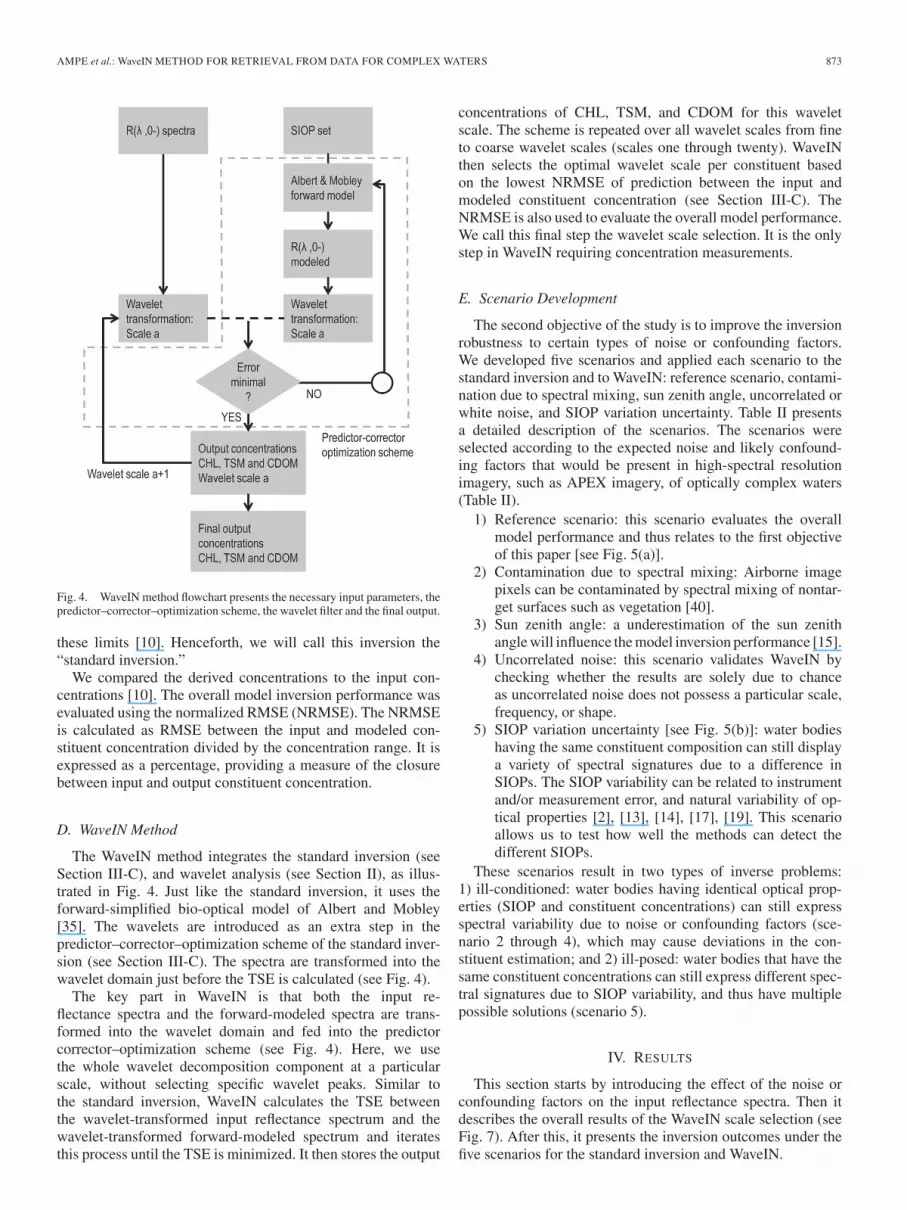
Fig. 4. WaveIN method flowchart presents the necessary input parameters, thepredictor–corrector–optimization scheme, the wavelet filter and the final output.

these limits [10]. Henceforth, we will call this inversion the“standard inversion.”

We compared the derived concentrations to the input con-centrations [10]. The overall model inversion performance wasevaluated using the normalized RMSE (NRMSE). The NRMSEis calculated as RMSE between the input and modeled con-stituent concentration divided by the concentration range. It isexpressed as a percentage, providing a measure of the closurebetween input and output constituent concentration.

D. WaveIN Method

The WaveIN method integrates the standard inversion (seeSection III-C), and wavelet analysis (see Section II), as illus-trated in Fig. 4. Just like the standard inversion, it uses theforward-simplified bio-optical model of Albert and Mobley[35]. The wavelets are introduced as an extra step in thepredictor–corrector–optimization scheme of the standard inver-sion (see Section III-C). The spectra are transformed into thewavelet domain just before the TSE is calculated (see Fig. 4).

The key part in WaveIN is that both the input re-flectance spectra and the forward-modeled spectra are trans-formed into the wavelet domain and fed into the predictorcorrector–optimization scheme (see Fig. 4). Here, we usethe whole wavelet decomposition component at a particularscale, without selecting specific wavelet peaks. Similar tothe standard inversion, WaveIN calculates the TSE betweenthe wavelet-transformed input reflectance spectrum and thewavelet-transformed forward-modeled spectrum and iteratesthis process until the TSE is minimized. It then stores the output

concentrations of CHL, TSM, and CDOM for this waveletscale. The scheme is repeated over all wavelet scales from fineto coarse wavelet scales (scales one through twenty). WaveINthen selects the optimal wavelet scale per constituent basedon the lowest NRMSE of prediction between the input andmodeled constituent concentration (see Section III-C). TheNRMSE is also used to evaluate the overall model performance.We call this final step the wavelet scale selection. It is the onlystep in WaveIN requiring concentration measurements.

E. Scenario Development

The second objective of the study is to improve the inversionrobustness to certain types of noise or confounding factors.We developed five scenarios and applied each scenario to thestandard inversion and to WaveIN: reference scenario, contami-nation due to spectral mixing, sun zenith angle, uncorrelated orwhite noise, and SIOP variation uncertainty. Table II presentsa detailed description of the scenarios. The scenarios wereselected according to the expected noise and likely confound-ing factors that would be present in high-spectral resolutionimagery, such as APEX imagery, of optically complex waters(Table II).

1) Reference scenario: this scenario evaluates the overallmodel performance and thus relates to the first objectiveof this paper [see Fig. 5(a)].

2) Contamination due to spectral mixing: Airborne imagepixels can be contaminated by spectral mixing of nontar-get surfaces such as vegetation [40].

3) Sun zenith angle: a underestimation of the sun zenithangle will influence the model inversion performance [15].

4) Uncorrelated noise: this scenario validates WaveIN bychecking whether the results are solely due to chanceas uncorrelated noise does not possess a particular scale,frequency, or shape.

5) SIOP variation uncertainty [see Fig. 5(b)]: water bodieshaving the same constituent composition can still displaya variety of spectral signatures due to a difference inSIOPs. The SIOP variability can be related to instrumentand/or measurement error, and natural variability of op-tical properties [2], [13], [14], [17], [19]. This scenarioallows us to test how well the methods can detect thedifferent SIOPs.

These scenarios result in two types of inverse problems:1) ill-conditioned: water bodies having identical optical prop-erties (SIOP and constituent concentrations) can still expressspectral variability due to noise or confounding factors (sce-nario 2 through 4), which may cause deviations in the con-stituent estimation; and 2) ill-posed: water bodies that have thesame constituent concentrations can still express different spec-tral signatures due to SIOP variability, and thus have multiplepossible solutions (scenario 5).

IV. RESULTS

This section starts by introducing the effect of the noise orconfounding factors on the input reflectance spectra. Then itdescribes the overall results of the WaveIN scale selection (seeFig. 7). After this, it presents the inversion outcomes under thefive scenarios for the standard inversion and WaveIN.

874 IEEE TRANSACTIONS ON GEOSCIENCE AND REMOTE SENSING, VOL. 53, NO. 2, FEBRUARY 2015

TABLE IIDETAILED DESCRIPTION OF THE DIFFERENT SCENARIOS OF NOISE AND CONFOUNDING FACTORS

Fig. 5. Schematic representing WaveIN scenario 1 (reference scenario) andscenario 5 (SIOP variation uncertainty).

Figs. 8–12 visually compare the inversion outcomes for eachscenario. The gray-scale color indicates samples with a high ora low TSM concentration. WaveIN estimates the constituentsfor different wavelet scales ranked from one to twenty, for finewavelet scales (low rank) to coarse wavelet scales (higher rank),respectively. Note that the figures display only two relevantwavelet scales per scenario, this to convey the findings in aconsistent and reduced way. A detailed overview of the waveletscales selected per constituent is listed in Table IV.

As an approximation for the deviation between the empiricalslope and the 1:1 line, we discuss the slope difference. As anindicator of error variance, we discuss the spread of the datacloud. Models with a slope difference can still provide predic-tive power, whereas for erroneous models with low predictivepower the precision is compromised.

A. Effect of Noise or Confounding Factors on the InputReflectance Spectra

This section describes and visualizes the treatment of thedifferent scenarios on the input reflectance spectra. Since thescenarios are the same for all of the 1000 input reflectance

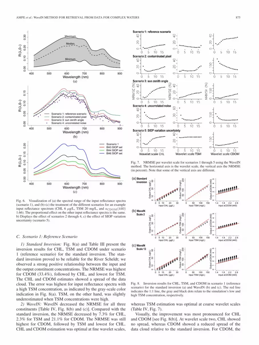
spectra, we will discuss the effect on one example spectrum.The median, maximum and minimum input reflectance spectraare displayed in Fig. 6(a). The spectral range is solely relatedto the input concentration range used to simulate the inputreflectance spectra (see Table I).

1) Scenario 2 Through 4: The contamination due to spectralmixing (scenario 2) caused a global increase in the inputreflectance spectra. The most notable increase was mainly inthe near infrared (NIR) and relatively limited in the blue wave-lengths, which is related to the spectral shape of a vegetationsignal. A change in sun zenith angle from 0◦ to 45◦ (scenario 3)caused a global increase in the reflectance signal [see Fig. 6(b)].The increase is uneven and most pronounced between 550 and700 nm. The effect of uncorrelated noise (scenario 4) is trivial.Uncorrelated noise introduced a random scattering around theinput reflectance spectrum [see Fig. 6(b)].

2) Scenario 5: The variation uncertainty in SIOPs (sce-nario 5) caused the largest deviation from the reference sce-nario (scenario 1). This effect was most pronounced in thegreen–red wavelengths due to the variation in a∗ph and b∗TSM

[see Fig. 6(c)]. BA3 and BA6 differed the most from thereference input spectrum [see Fig. 6(c)], because BA3 had thelowest a∗ph and b∗TSM, whereas BA6 had the highest b∗TSM.

B. Overall Results of the WaveIN Scale Selection

Fig. 7 presents the NRMSE of the estimation of CHL, TSM,and CDOM per wavelet scale for WaveIN. The NRMSE variedper wavelet scale for all three constituents. For CHL, exceptfor scenario 4 (uncorrelated noise), the NRMSE plots showeda similar trend for all of the scenarios: the NRMSE decreasedafter wavelet scale one and increased again after wavelet scalefive, reaching a minimum between wavelet scales two and five.For TSM, the NRMSE did not express a clear behavior overthe wavelet scales. Only scenario 2 and 3 showed for TSM aspecific behavior, where the NRMSE increased with increasingwavelet scale (see Fig. 7). For scenarios 1, 3, and 5, the NRMSEof CDOM showed a similar trend as for CHL. For CDOM,a minimum NRMSE is reached between wavelet scales twoand four.

AMPE et al.: WaveIN METHOD FOR RETRIEVAL FROM DATA FOR COMPLEX WATERS 875

Fig. 6. Visualization of (a) the spectral range of the input reflectance spectra(scenario 1), and (b)-(c) the treatment of the different scenarios for an exampleinput reflectance spectrum (CHL 6 μg/L, TSM 20 mg/L, and aCDOM(440)1.66). The proportional effect on the other input reflectance spectra is the same.b) Displays the effect of scenarios 2 through 4, c) the effect of SIOP variationuncertainty (scenario 5).

C. Scenario 1: Reference Scenario

1) Standard Inversion: Fig. 8(a) and Table III present theinversion results for CHL, TSM and CDOM under scenario1 (reference scenario) for the standard inversion. The stan-dard inversion proved to be reliable for the River Scheldt; weobserved a strong positive relationship between the input andthe output constituent concentrations. The NRMSE was highestfor CDOM (33.4%), followed by CHL, and lowest for TSM.The CHL and CDOM estimates showed a spread of the datacloud. The error was highest for input reflectance spectra witha high TSM concentration, as indicated by the gray-scale colorindication in Fig. 8(a). TSM, on the other hand, was slightlyunderestimated when TSM concentrations were high.

2) WaveIN: WaveIN decreased the NRMSE for all threeconstituents [Table IV, Fig. 8(b) and (c)]. Compared with thestandard inversion, the NRMSE decreased by 7.3% for CHL,2.3% for TSM and 21.1% for CDOM. The NRMSE was stillhighest for CDOM, followed by TSM and lowest for CHL.CHL and CDOM estimation was optimal at fine wavelet scales,

Fig. 7. NRMSE per wavelet scale for scenarios 1 through 5 using the WaveINmethod. The horizontal axis is the wavelet scale, the vertical axis the NRMSE(in percent). Note that some of the vertical axis are different.

Fig. 8. Inversion results for CHL, TSM, and CDOM in scenario 1 (referencescenario) for the standard inversion (a) and WaveIN (b) and (c). The red lineindicates the 1:1 line, the gray and black dots relate to the simulation’s low andhigh TSM concentration, respectively.

whereas TSM estimation was optimal at coarse wavelet scales(Table IV, Fig. 7).

Visually, the improvement was most pronounced for CHLand CDOM [see Fig. 8(b)]. At wavelet scale two, CHL showedno spread, whereas CDOM showed a reduced spread of thedata cloud relative to the standard inversion. For CDOM, the

876 IEEE TRANSACTIONS ON GEOSCIENCE AND REMOTE SENSING, VOL. 53, NO. 2, FEBRUARY 2015

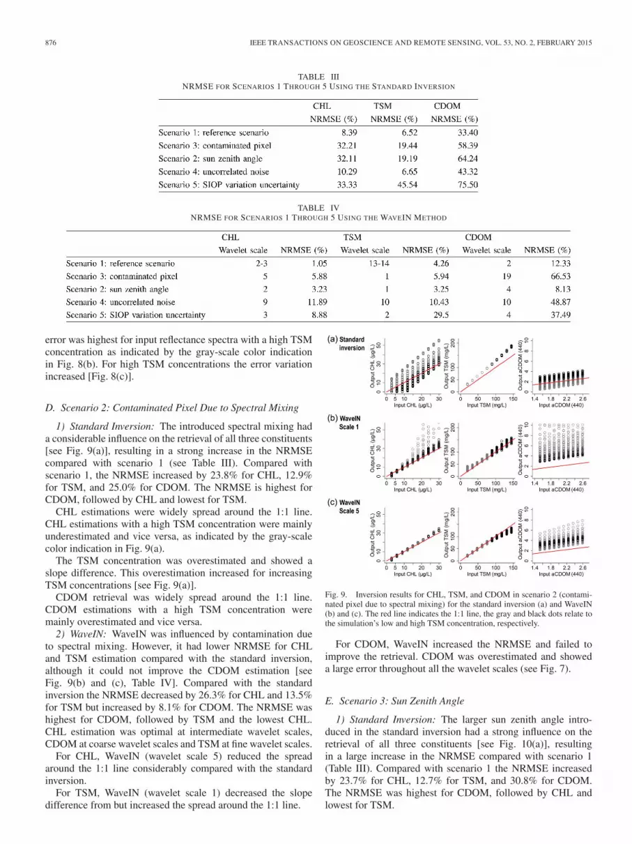
TABLE IIINRMSE FOR SCENARIOS 1 THROUGH 5 USING THE STANDARD INVERSION

TABLE IVNRMSE FOR SCENARIOS 1 THROUGH 5 USING THE WAVEIN METHOD

error was highest for input reflectance spectra with a high TSMconcentration as indicated by the gray-scale color indicationin Fig. 8(b). For high TSM concentrations the error variationincreased [Fig. 8(c)].

D. Scenario 2: Contaminated Pixel Due to Spectral Mixing

1) Standard Inversion: The introduced spectral mixing hada considerable influence on the retrieval of all three constituents[see Fig. 9(a)], resulting in a strong increase in the NRMSEcompared with scenario 1 (see Table III). Compared withscenario 1, the NRMSE increased by 23.8% for CHL, 12.9%for TSM, and 25.0% for CDOM. The NRMSE is highest forCDOM, followed by CHL and lowest for TSM.

CHL estimations were widely spread around the 1:1 line.CHL estimations with a high TSM concentration were mainlyunderestimated and vice versa, as indicated by the gray-scalecolor indication in Fig. 9(a).

The TSM concentration was overestimated and showed aslope difference. This overestimation increased for increasingTSM concentrations [see Fig. 9(a)].

CDOM retrieval was widely spread around the 1:1 line.CDOM estimations with a high TSM concentration weremainly overestimated and vice versa.

2) WaveIN: WaveIN was influenced by contamination dueto spectral mixing. However, it had lower NRMSE for CHLand TSM estimation compared with the standard inversion,although it could not improve the CDOM estimation [seeFig. 9(b) and (c), Table IV]. Compared with the standardinversion the NRMSE decreased by 26.3% for CHL and 13.5%for TSM but increased by 8.1% for CDOM. The NRMSE washighest for CDOM, followed by TSM and the lowest CHL.CHL estimation was optimal at intermediate wavelet scales,CDOM at coarse wavelet scales and TSM at fine wavelet scales.

For CHL, WaveIN (wavelet scale 5) reduced the spreadaround the 1:1 line considerably compared with the standardinversion.

For TSM, WaveIN (wavelet scale 1) decreased the slopedifference from but increased the spread around the 1:1 line.

Fig. 9. Inversion results for CHL, TSM, and CDOM in scenario 2 (contami-nated pixel due to spectral mixing) for the standard inversion (a) and WaveIN(b) and (c). The red line indicates the 1:1 line, the gray and black dots relate tothe simulation’s low and high TSM concentration, respectively.

For CDOM, WaveIN increased the NRMSE and failed toimprove the retrieval. CDOM was overestimated and showeda large error throughout all the wavelet scales (see Fig. 7).

E. Scenario 3: Sun Zenith Angle

1) Standard Inversion: The larger sun zenith angle intro-duced in the standard inversion had a strong influence on theretrieval of all three constituents [see Fig. 10(a)], resultingin a large increase in the NRMSE compared with scenario 1(Table III). Compared with scenario 1 the NRMSE increasedby 23.7% for CHL, 12.7% for TSM, and 30.8% for CDOM.The NRMSE was highest for CDOM, followed by CHL andlowest for TSM.

AMPE et al.: WaveIN METHOD FOR RETRIEVAL FROM DATA FOR COMPLEX WATERS 877

Fig. 10. Inversion results for CHL, TSM, and CDOM in scenario 3 (sun zenithangle) for the standard inversion (a) and WaveIN (b) and (c). The red lineindicates the 1:1 line, the gray and black dots relate to the simulation’s lowand high TSM concentration, respectively.

CHL showed a wide spread around the 1:1 line, and wasunderestimated; this underestimation was most pronounced forCHL estimations with a high TSM concentration, as indicatedby the gray-scale color indication in Fig. 10(a).

The TSM concentration was overestimated and showed aslope difference. This overestimation increased for increasingTSM concentrations [Fig. 10(a)].

CDOM retrieval was widely spread around the 1:1 line[Fig. 10(a)].

2) WaveIN: WaveIN decreased the NRMSE for CHL,TSM, and CDOM compared with the standard inversion [seeFig. 10(b) and (c), Table IV]. Compared with the standardinversion, the NRMSE decreased by 28.9% for CHL, 15.9%for TSM, and 56.1% for CDOM. The NRMSE was highest forCDOM, followed by TSM and lowest for CHL. CHL, TSM andCDOM estimation was optimal at relatively fine wavelet scales.

For CHL, WaveIN does not underestimate the concentration.The estimates lie close to the 1:1 line. WaveIN selected thesame wavelet scale as in scenario 1.

The TSM estimates lie closer to the 1:1 line than in thestandard inversion. Nevertheless, for TSM, the sun zenithangle resulted in an increased error variation for high TSMconcentrations.

For CDOM, WaveIN strongly decreased the spread aroundthe 1:1 line [Fig. 10(c)].

F. Scenario 4: Uncorrelated Noise

1) Standard Inversion: The uncorrelated noise we intro-duced increased the NRMSE of the standard inversion for allthree constituents compared with scenario 1 [see Fig. 11(a)] andTable III). Compared with scenario 1, the NRMSE increasedby 1.9% for CHL, 0.1% for TSM, and 9.9% for CDOM. TheNRMSE was highest for CDOM, followed by CHL and lowestfor TSM.

Fig. 11. Inversion results for CHL, TSM, and CDOM in scenario 4 (uncorre-lated noise) for the standard inversion (a) and WaveIN (b) and (c). The red lineindicates the 1:1 line, the gray and black dots relate to the simulation’s low andhigh TSM concentration, respectively.

For CHL the uncorrelated noise caused considerable spreadaround the 1:1 line. Furthermore, this resulted in a reduceddifferentiation of samples with respect to high or low TSMconcentration, as indicated by the gray-scale color indication[see Fig. 11(a)].

The effect of uncorrelated noise on the TSM estimation waslimited. Nevertheless, for TSM, the uncorrelated noise resultedin an increased error variation for high TSM concentrations [seeFig. 11(a)].

For CDOM, the uncorrelated noise resulted in an increasedspread around the 1:1 line [see Fig. 11(a)].

2) WaveIN: WaveIN could not improve the constituent es-timation and caused an increase of the NRMSE for all threeconstituents [see Fig. 11(b) and (c), Table IV]. Compared withthe standard inversion, the NRMSE increased by 1.6% for CHL,3.8% for TSM, and 5.6% for CDOM. The NRMSE was stillhighest for CDOM, followed by CHL and lowest for TSM. Allthree constituents were best estimated at intermediate waveletscales.

For CHL and CDOM, we observed similar, but morepronounced spread around the 1:1 line as for the standardinversion.

For TSM, WaveIN caused spread around the 1:1 line and astrong increase in the error variation from low to high TSMconcentrations.

G. Scenario 5: SIOP Variation Uncertainty

1) Standard Inversion: The SIOP variation uncertainty in-troduced in the standard inversion had a considerable influ-ence on the retrieval of all three constituents [see Fig. 12(a),Table III] and resulted in an increase in the NRMSE of allthree constituents. Compared with scenario 1, the NRMSEincreased by 24.9% for CHL, 39.0% for TSM, and 42.1% forCDOM. The NRMSE was still highest for CDOM, followed

878 IEEE TRANSACTIONS ON GEOSCIENCE AND REMOTE SENSING, VOL. 53, NO. 2, FEBRUARY 2015

Fig. 12. Inversion results for CHL, TSM, and CDOM in scenario 5 (SIOPvariation uncertainty) for the standard inversion (a) and WaveIN (b) and (c).The red line indicates the 1:1 line, the colors are related to the input SIOP set(black: average SIOP set, red: BA3 SIOP set, green: BA4 SIOP, and blue: BA6SIOP set).

by TSM and lowest for CHL. Fig. 12 clearly discriminatesthe groups of samples derived from a different SIOP set. Thebest estimation was obtained for the average SIOP set, whichis, in fact, scenario 1. The BA6 SIOP set, showed the largestdeviation, which was related to the high specific TSM scatteringcoefficients (see Fig. 2).

For CHL, the SIOPs variation uncertainty resulted in consid-erable spread around the 1:1 line. We could clearly discriminatethe different samples according to their input SIOP set.

For TSM, the spectral variation resulted in higher errorvariation for high TSM concentrations. In this case, the errorvariation is related to the different input SIOPs. Each SIOPinput set strongly influenced the slope between the input andoutput TSM concentration.

For CDOM, this spectral variation resulted in considerablespread around the 1:1 line. However, we could not clearlydistinguish the different samples according to their inputSIOP set.

2) WaveIN: WaveIN decreased the NRMSE for all threeconstituents and thus improved the constituent retrieval com-pared with the standard inversion [see Table IV, Fig. 12(b)and (c)]. Compared with the standard inversion, the NRMSEdecreased by 24.5% for CHL, 16.0% for TSM, and 38.0% forCDOM. The NRMSE was still highest for CDOM, followedby TSM and lowest for CHL. All three constituents were bestestimated at relatively fine wavelet scales.

For CHL, WaveIN decreased the spread around the 1:1 line[see Fig. 12(b)]. The optimal wavelet scale was the sameas in scenario 1 (reference scenario). Visually, the separationbetween the SIOP input sets has been reduced.

For TSM, WaveIN decreased the error variation from lowto high TSM concentrations and reduced the slope difference.However, a considerable difference between the SIOP sets anda high NRMSE compared with scenario 1 still remained.

For CDOM, WaveIN decreased the spread around the 1:1line [see Fig. 12(c)]. Note, we could not sufficiently evaluatethe influence of SIOP variation uncertainty on the CDOMestimation as we only obtained one usable CDOM sample.

V. DISCUSSION

A. WaveIN Scale Selection

The NRMSE of the constituent retrieval varied over thewavelet scales and scenarios (see Fig. 7). Here, we will notdiscuss the results of Scenario 4, since it is developed toverify the assumptions of WaveIN and to check if the solutionwas solely due to chance (see Section V-E in the succeedingdiscussion). The consistent behavior of the NRMSE of CHL(see Fig. 7) is straightforward since it is the only variablewith distinct and spectrally localized features [12], [41]. CHLis therefore best estimated at fine wavelet scales, which is inagreement with the observations of Ampe et al. [12]. The scaleselection of TSM and CDOM is less specific (see Fig. 7). Thespectral effect of CDOM is subtle and that of TSM broad, whichmeans the effect will be present at most of the wavelet scales.

The reliance on in situ data for wavelet scale selection,and the selection of one optimal wavelet scale per constituent,makes the method a combination of a semianalytical inversionwith a semiempirical wavelet scale selection. Fig. 7 shows agradual change in the NRMSE over the wavelet scales. Thisindicates a promising potential future development toward anapproach that is semianalytical and extensible: a multiscaleapproach that uses the weighted average of interesting waveletscales for the different constituents. Such an approach wouldovercome the problem of picking one single wavelet scale forone specific scenario. Future research should further investigatethe consistent behavior of the NRMSE over the different wave-lengths and scenarios (see Fig. 7) and verify this for differentdata sets, both air- and spaceborne. If this behavior persists,one could define a sensor specific wavelet scale selection ap-proach. We envision an improved WaveIN algorithm that takesa weighted average of the wavelet scales, which have previouslybeen defined as interesting for a specific sensor and study area.

Due to model errors, noise, or confounding factors, thespectral features of the input reflectance spectrum may change,resulting in imperfect optical closure [6], [9], [12], [42]. Be-cause of poor optical closure, the best fitting solution maynot result in accurate estimation of the concentrations [6]. Forexample, where we had high TSM concentration, the standardinversion could not correctly match reflectance with the correctCHL concentration because the standard inversion optimizesthe overall spectral shape. WaveIN was more successful atCHL concentration retrieval under high TSM conditions be-cause WaveIN focuses the optimization per wavelet scale. Atfine wavelet scales, the CHL spectral features are enhanced,improving CHL concentration retrieval [12]. In such a case,WaveIN mainly matches the CHL spectral features and, to alesser extent, the signal magnitude, which may in some casesreduce TSM concentration retrieval. Essentially, in the waveletdomain, certain spectral features are enhanced, and we can findthe optimal fit for those features although in the wavelengthdomain the optical closure might be suboptimal.

AMPE et al.: WaveIN METHOD FOR RETRIEVAL FROM DATA FOR COMPLEX WATERS 879

WaveIN’s selective optimization per constituent in thewavelet domain overcomes some of the retrieval errors due topoor optical closure in the wavelength domain. However, thismeans that WaveIN is not simultaneously retrieving all of theconstituents. This is still an ongoing issue; a few studies ininland waters successfully solve for all three constituents [4],[9], and validation is often only a minor part of the study [4],[6], [14]. We hypothesize that in complex waters, it might, insome cases, be difficult to correctly retrieve all the constituentssimultaneously. A model that enhances the CHL features mayimpede the estimation of other constituents.

B. Scenario 1: Reference Scenario

1) Standard Inversion: The standard inversion proves to bea reliable method for this study area in the case of good qualityreflectance data. The slight increase in error for high TSM con-centrations could be related to the calibration of the forward-simplified bio-optical model of Albert and Mobley [35], whichwas limited to a TSM concentration of 50 mg/L. Furthermore,at high TSM concentrations, the scattering features of TSMbecome dominant, impeding CHL and CDOM, resulting in anunderestimation of CHL and an overestimation of CDOM.

Our results demonstrate the importance of defining the sen-sitivity, and upper and lower theoretical bounds of both algo-rithms and sensors [15]. As previously discussed, the selectedstandard inversion becomes less accurate for high TSM con-centrations. In addition, the high TSM concentration influencesthe estimation of CHL and CDOM. Therefore, we would advisecare in using the standard inversion for more turbid waters. It isimportant to realize this in the development of new algorithmsfor complex waters.

2) WaveIN: WaveIN improved the estimation of all threeconstituents because wavelets decouple the combined and in-teracting influence of the constituents. The results confirm thehypothesis of Ampe et al. [12] that the optically active con-stituents influence the signal at various wavelet scales. In ourcase CHL was better estimated by fine wavelet scales becausethese absorption features are relatively narrow compared withthe coarse or broad effect of scattering by TSM (see Fig. 2).WaveIN can decompose the information content and enhancethe spectral feature recognition during optimization. This isuseful for optically complex waters especially those where highTSM concentration may mask the spectral features of otherconstituents [3], [4].

C. Scenario 2: Contaminated Pixel Due to Spectral Mixing

1) Standard Inversion: Under scenario 2, the standard in-version had high errors in the estimation of the constituentconcentrations (Table III). The global spectral increase plusthe deformation of the spectral features caused problems inthe spectral matching of the predictor–corrector optimizationscheme. Furthermore, the increase in spectral signature due toscenario 2 caused TSM overestimation.

2) WaveIN: WaveIN improved the estimation of CHL andTSM but could not improve the estimation of CDOM. Thisis related to the way wavelets are calculated. At the edgeof the spectrum, the wavelet filter can only partly cover thespectrum as there are not enough spectral bands left. Therefore,

the wavelet filter uses spectral bands of the other side of thespectrum to fill these gaps. Since the mixing with a vegetationsignal caused a higher increase in the NIR than in the visualwavelengths, the wavelet decomposition showed considerableedge effects. For fine wavelet scales, these edge effects only in-fluence the outer wavelengths. This becomes more pronouncedat coarser wavelet scales. Hence, WaveIN is sensitive to thelocation of the spectral features within the overall spectralsignature. However, WaveIN can select the wavelet scale, wherethe feature contamination was minimal. Wavelet edge effectscould be identified by defining the cone of influence (COI) ofthe wavelet filter. The spectral bands influenced by the COIcould later on be removed from the analysis. Furthermore, theproblem of wavelet edge effects could be mitigated by selectinga wider wavelength range, which could dilute the edge effects orby using an edge avoiding technique, such as second-generationwavelet analysis [43].

CHL spectral features were not located near the edge of theinput reflectance spectrum and were best preserved at interme-diate wavelet scales. Although the mixture with a vegetationsignal caused a deformation in the spectral features, WaveINcould avoid this by selecting a coarser wavelet scale thanin scenario 1. Additionally, wavelets are less sensitive to thevertical displacement of the signal and focus on the spectralshape [12]. By definition, wavelet analysis is blind to a verticaldisplacement of a signal because wavelets must have zerointegrals [44].

CDOM absorption is mainly present at short wavelengths(see Fig. 2), where the wavelet edge effects were most pro-nounced, which explains why WaveIN could not improve theCDOM estimation.

In contrast to scenario 1, TSM estimation was optimal hereat a fine wavelet scale. This is because TSM influences theoverall spectral signature. The wavelet edge effects becamemore pronounced at these coarse wavelet scales. Therefore,WaveIN avoided these scales by selecting a fine wavelet scale.

In the future, we could investigate if WaveIN also improvesestimations of spectra influenced by adjacency effects, as thisalso strongly influences the NIR wavelengths [45]. Therefore, itwould be useful to test WaveIN on airborne imagery, for whichwe need a large set of coupled in-water and remote sensingmeasurements.

D. Scenario 3: Sun Zenith Angle

1) Standard Inversion: Under scenario 3, the standard in-version estimated the constituent concentration with a largeerror. Analogous to scenario 2, the global spectral increase plusthe deformation of the spectral features caused problems inthe spectral matching of the predictor–corrector optimizationscheme. However, again, the increase in spectral signature isthe reason TSM was overestimated. This strong influence ofthe sun zenith angle demonstrates the importance of algorithmsthat can cope with noisy data. In many occasions, the influenceof the sun angle or atmosphere may overrule the signal-to-noiseratio of the sensor.

2) WaveIN: WaveIN could improve the estimation of allthree constituents. As in scenario 2, a change in sun zenithangle caused a variable global increase in the spectral signature.However, in this case, there were less wavelet edge effects as

880 IEEE TRANSACTIONS ON GEOSCIENCE AND REMOTE SENSING, VOL. 53, NO. 2, FEBRUARY 2015

there was only a limited difference between the increase inthe NIR and the visual wavelengths. Furthermore, if we wouldconcentrate on short wavelength intervals, scenario 3 resemblesa vertical bias. As discussed in scenario 2, by definition, waveletanalysis is blind to a vertical displacement of a signal [44].

For CHL, WaveIN selected the same wavelet scale as inscenario 1. The reason for this is twofold: 1) CHL spectralfeatures are localized and not located near the edge of the inputreflectance spectrum, they are therefore less affected by waveletedge effects; and 2) as discussed in the previous paragraph, weexpect less influence of the wavelet edge effects compared withscenario 2.

For TSM, we can draw the same conclusions as in scenario2. Due to the wavelet edge effects, the optimal wavelet scaleshifted toward fine wavelet scales. As previously discussed, forthis scenario, the wavelet edge effect is limited compared withscenario 2. However, for TSM this effect remains strong enoughto influence the wavelet scale selection.

The estimation of CDOM was less affected by the waveletedge effects compared with scenario 2. As previously dis-cussed, for this scenario the wavelet edge effect is limitedcompared with scenario 2. In addition, the shift in optimalwavelet scale was limited. The wavelet scale selection forCDOM was less affected by the edge effect than it was for TSM.

E. Scenario 4: Uncorrelated Noise

The random effects in the spectral signature made it dif-ficult for the standard inversion to correctly match the inputand forward-modeled spectra. WaveIN could not improve con-stituent retrieval because wavelets cannot avoid uncorrelatednoise as uncorrelated noise does not possess a particular scale,frequency or shape. We added this scenario to verify the as-sumptions of WaveIN and to check if the solution was solelydue to chance. The effect of uncorrelated noise could be tackledby other techniques, such as presmoothing using splines orkernel methods [46].

F. Scenario 5: SIOP Variation Uncertainty

1) Standard Inversion: Under scenario 5, the standard inver-sion produced a large error in the estimation of the constituents.The variation in SIOPs of the target water body caused spectralvariation. This ill-posedness is clearly visible in the result asit impedes correct spectral matching in the predictor–correctoroptimization scheme.

2) WaveIN: WaveIN improved the estimation of the threeconstituents in this ill-posed problem. The reason is similarfor all three constituents. WaveIN could avoid the change inspectral features by selecting optimal wavelet scales wherethis influence is minimal and wavelets are less sensitive to thevertical displacement in the spectral signature.

Still, WaveIN could not solve the problem of the influenceof SIOP variability. SIOP variability is a key problem in in-verse modeling of remote sensing data [2], [18], which cannotbe overlooked. For future research, we propose to combineWaveIN with an adaptive approach [2]. In addition, we shouldtest this methodology on an independent data set or differentgeographical location with different SIOP variability [17].

G. Overall Discussion

The generally positive effects of WaveIN on the multiscaleestimation of optically active constituents contribute to thepresent knowledge in semianalytical modeling [4]. Due to itsobject-oriented nature, WaveIN can easily be integrated withother semianalytical inversion models or LUT approaches [47].A different (nonwavelet) multiscale approach was introducedby Sadeghi et al. [48] and Bracher et al. [49] and demonstratedthe effectiveness of scale space for aquatic optical remotesensing. They improved the identification of phytoplanktonfunctional types by separating the higher frequency absorptionstructures from broad band features through the subtractionof a polynomial for different wavelength windows. They usedthe whole spectral wavelength range as opposed to specificwavelengths to calculate the phytoplankton group biomass.Giardino et al. [9] approached the large number of Hyperionbands in the matrix inversion method via a sensitivity analysis[47]. They have found Hyperion too noisy and ill-calibratedin the shortest wavelengths where CDOM variation was thehighest and where therefore unable to estimate CDOM. Modelinversion using neural networks [7], [8] has been proposed asa method less sensitive to noise [50]. These methods howeverneed ample training data [51] and may have problems inextrapolation far away outside the subspace of the trainingdata [52], [53]. Support vector machine have been proposedto overcome these problems, but further research is needed[50], [51]. For multispectral measurements such as MERIS, theprincipal component inversion (PCI) [54] has been developedwith an internal training scheme based on principal componentanalysis, which extracts the most informative part of the dataset. The method should reduce the dependency on measurementnoise [54]. The applicability of PCI on high-spectral resolutiondata and the influence of other confounding factors should befurther be investigated [55].

VI. CONCLUSION AND OUTLOOK

We have proposed WaveIN as a novel inversion technique toestimate the CHL, TSM and CDOM concentration from high-spectral resolution data in complex waters. WaveIN is basedon a predictor–corrector optimization scheme and uses wavelet-transformed spectra, instead of the original high-spectral reso-lution reflectance signal. WaveIN was able to partly resolve thetwo objectives of this paper 1) to improve bio-optical inversionresults in estimating the optically active constituents CHL,TSM, and CDOM; and 2) to improve the model robustness tocertain types of noise or confounding factors. WaveIN had apositive effect on the estimation of CHL, TSM, and CDOM inthe case of the reference scenario, and for most of the scenarios.However, although WaveIN reduced the influence of variationin SIOPs, it could not completely resolve it. The multiscaleapproach is a powerful tool for enhanced information extrac-tion as wavelets can decouple the combined influence of theconfounding factors. Additionally, wavelets are less sensitiveto a bias in the spectra and can avoid the changing or shiftingspectral features by selecting specific wavelet scales.

The obvious next step is to test this methodology onAPEX imagery. Here, one should first define the optimalwavelet scales based on the in situ concentration measurements.These measurements should be spatially distributed to capture

AMPE et al.: WaveIN METHOD FOR RETRIEVAL FROM DATA FOR COMPLEX WATERS 881

different types of image contamination. The waveIN methodis therefore not fully analytical as it will need in situ datato select the best wavelet scales. Additional research shouldfocus on various air- or spaceborne optical remote sensing dataand additional types of noise and confounding factors, e.g.,adjacency effect, high-frequency noise, atmospheric noise, andsky glint. Future studies on real images should also improvethe wavelet scale selection. Instead of selecting one optimalwavelet scale, one should investigate a weighted average of acluster of informative wavelet scales per constituent.

ACKNOWLEDGMENT

The authors would like to thank the partners in the MICASproject for their significant contributions in the fieldwork anddata analysis. The authors also thank L. Bertels, P. Grötsch,K. Hestir, J. Nossent, and the two anonymous reviewers fortheir useful comments and suggestions.

REFERENCES

[1] C. D. Mobley, “Optical Properties ofWater,” in Handbook of Optics,2nd ed. New York, NY, USA: McGraw-Hill, 1994..

[2] V. E. Brando, A. G. Dekker, Y. J. Park, and T. Schroeder, “Adaptivesemi-analytical inversion of ocean color radiometry in optically complexwaters,” Appl. Opt., vol. 51, no. 15, pp. 2808–2833, May 2012.

[3] M. W. Matthews, “A current review of empirical procedures of remotesensing in inland and near-coastal transitional waters,” Int. J. RemoteSens., vol. 32, no. 21, pp. 6855–6899, 2011.

[4] D. Odermatt, A. Gitelson, V. E. Brando, and M. Schaepman, “Review ofconstituent retrieval in optically deep and complex waters from satelliteimagery,” Remote Sens. Environ., vol. 118, pp. 116–126, Mar. 2012.

[5] S. Maritorena, D. A. Siegel, and A. R. Peterson, “Optimization of asemianalytical ocean color model for global-scale applications,” Appl.Opt., vol. 41, no. 15, pp. 2705–2714, May 2002.

[6] H. J. van der Woerd and R. Pasterkamp, “HYDROPT: A fast and flexiblemethod to retrieve chlorophyll-a from multispectral satellite observationsof optically complex coastal waters,” Remote Sens. Environ., vol. 112,no. 4, pp. 1795–1807, Apr. 2008.

[7] L. González Vilas, E. Spyrakos, and J. M. Torres Palenzuela, “Neuralnetwork estimation of chlorophyll a from MERIS full resolution data forthe coastal waters of Galician rias (NW Spain),” Remote Sens. Environ.,vol. 115, no. 2, pp. 524–535, Feb. 2011.

[8] R. Doerffer and H. Schillera, “The MERIS case 2 water algorithm,” Int.J. Remote Sens., vol. 28, no. 3/4, pp. 517–535, Feb. 2007.

[9] C. Giardino, V. E. Brando, A. Dekker, N. Strombeck, and G. Candiani,“Assessment of water quality in Lake Garda (Italy) using hyperion,”Remote Sens. Environ., vol. 109, no. 2, pp. 183–195, Jul. 2007.

[10] Z. Lee, K. L. Carder, C. D. Mobley, R. G. Steward, and J. S. Patch,“Hyperspectral remote sensing for shallow waters: 2. Deriving bottomdepths and water properties by optimization,” Appl. Opt., vol. 38, no. 18,pp. 3831–3943, Jun. 1999.

[11] Z. P. Lee, K. Carder, T. Peacock, C. O. Davis, and J. L. Mueller, “Methodto derive ocean absorption coefficients from remote-sensing reflectance,”Appl. Opt., vol. 35, no. 3, pp. 453–462, Jan. 1996.

[12] E. M. Ampe et al., “A wavelet approach for estimating chlorophyll-a frominland waters with reflectance spectroscopy,” IEEE Geosci. Remote Sens.Lett., vol. 11, no. 1, pp. 89–93, Jan. 2014.

[13] G. Dall’Olmo and A. A. Gitelson, “Effect of bio-optical parametervariability and uncertainties in reflectance measurements on the remoteestimation of chlorophyll-a concentration in turbid productive waters:Modeling results,” Appl. Opt., vol. 45, no. 15, pp. 3577–3592, May 2006.

[14] T. J. Malthus, E. L. Hestir, A. Dekker, and V. E. Brando, “The case fora global inland water quality product,” in Proc. IEEE IGARSS, Munich,Germany, Jul. 22–27, 2012, pp. 5234–5237.

[15] J. D. Hedley, C. M. Roelfsema, S. R. Phinn, and P. J. Mumby, “Envi-ronmental and sensor limitations in optical remote sensing of coral reefs:Implications for monitoring and sensor design,” Remote Sens., vol. 4,no. 1, pp. 271–302, 2012.

[16] S. I. Kabanikhin, “Defnitions and examples of inverse and ill-posed prob-lems,” J. Inverse Ill-posed Problems, vol. 16, pp. 317–357, 2008.

[17] G. H. Tilstone et al., “Variability in specific-absorption properties andtheir use in a semi-analytical ocean colour algorithm for MERIS in NorthSea and Western English Channel Coastal Waters,” Remote Sens. Envi-ron., vol. 118, pp. 320–338, 2012.

[18] P. Wang, E. Boss, and C. Roesler, “Uncertainties of inherent opticalproperties obtained from semianalytical inversions of ocean color,” Appl.Opt., vol. 44, no. 19, pp. 4074–4084, 2005.

[19] G. Campbell and S. R. Phinn, “An assessment of the accuracy and pre-cision of water quality parameters retrieved with the matrix inversionmethod,” Limnology Oceanogr.: Methods, vol. 8, pp. 16–29, 2010.

[20] B. Rivard, J. Feng, A. Gallie, and A. Sanchez Azofeifa, “Continuouswavelets for the improved use of spectral libraries and hyperspectral data,”Remote Sens. Environ., vol. 112, no. 6, pp. 2850–2862, Jun. 2008.

[21] T. Cheng, B. Rivard, and G. A. Sánchez Azofeifa, “Spectroscopic deter-mination of leaf water content using continuous wavelet analysis,” RemoteSens. Environ., vol. 115, no. 2, pp. 659–670, Feb. 2011.

[22] A. Chambolle, R. A. De Vore, N. Y. Lee, and B. J. Lucier, “Nonlinearwavelet image processing: variational problems, compression, and noiseremoval through wavelet shrinkage,” IEEE Trans. Image Process., vol. 7,no. 3, pp. 319–335, Mar. 1998.

[23] I. Daubechies, M. Defrise, and C. De Mol, “An iterative thresholding al-gorithm for linear inverse problems with a sparsity constraint,” Commun.Pure Appl. Math., vol. 57, no. 11, pp. 1413–1457, Nov. 2004.

[24] C. D. Mobley et al., “Comparison of numerical models for computingunderwater light fields,” Appl. Opt., vol. 32, no. 36, pp. 7484–7504,Dec. 1993.

[25] C. D. Mobley, Light and Water-Radiative Transfer in Natural Waters.San Diego, CA, USA: Academic, 1994.

[26] T. Cheng, B. Rivard, G. A. Sánchez Azofeifa, J. Feng, and M. CalvoPolanco, “Continuous wavelet analysis for the detection of green attackdamage due to mountain pine beetle infestation,” Remote Sens. Environ.,vol. 114, no. 4, pp. 899–910, Apr. 2010.

[27] S. Muraki, “Multiscale volume representation by a DoG wavelet,” IEEETrans. Vis. Comput. Graphics, vol. 1, no. 2, pp. 109–116, Apr. 1995.

[28] K. S. Schmidt and A. K. Skidmore, “Smoothing vegetation spectra withwavelets,” Int. J. Remote Sens., vol. 25, no. 6, pp. 1167–1184, 2004.

[29] D. L. Donoho and I. M. Johnstone, “Ideal spatial adaptation via waveletshrinkage,” Biometrika, vol. 81, no. 3, pp. 425–455, 1994.

[30] M. Chabert, J.-Y. Tourneret, and F. Castanie, “Time-scale analysis ofabrupt changes corrupted by multiplicative noise,” Signal Process.,vol. 80, no. 3, pp. 397–411, Mar. 2000.

[31] W. Baeyens, B. van Eck, C. Lambert, R. Wollast, and L. Goeyens, “Gen-eral description of the Scheldt estuary,” Hydrobiologia, vol. 366, no. 1–3,pp. 1–14, 1997.

[32] E. Knaeps, A. I. Dogliotti, D. Raymaekers, K. Ruddick, and S. Sterckx,“In situ evidence of non-zero reflectance in the OLCI 1020 nm band for aturbid estuary,” Remote Sens. Environ., vol. 120, pp. 133–144, Mar. 2012.

[33] Z. Lee, K. L. Carder, C. D. Mobley, R. G. Steward, and J. S. Patch,“Hyperspectral remote sensing for shallow waters. I. A semianalyticalmodel,” Appl. Opt., vol. 37, no. 27, pp. 6329–6338, Sep. 1998.

[34] K. I. Itten et al., “APEX—The Hyperspectral ESA Airborne Prism Exper-iment,” Sensors, vol. 8, no. 10, pp. 6235–6259, 2008.

[35] A. Albert and C. Mobley, “An analytical model for subsurface irradianceand remote sensing reflectance in deep and shallow case-2 waters,” Opt.Exp., vol. 11, no. 22, pp. 2873–2890, 2003.

[36] A. Albert and P. Gege, “Inversion of irradiance and remote sensing re-flectance in shallow water between 400 and 800 nm for calculations ofwater and bottom properties,” Appl. Opt., vol. 45, no. 10, pp. 2331–2343,Apr. 2006.

[37] R. M. Pope and E. S. Fry, “Absorption spectrum (380–700 nm) of pure wa-ter. II. Integrating cavity measurements,” Applied Optics, vol. 36, no. 33,pp. 8710–8723, 1997.

[38] A. Morel, “Optical properties of pure water and pure sea water,” in Op-tical Aspects of Oceanography. New York, NY, USA: Academic, 1974,pp. 1–24.

[39] L. S. Lasdon, A. D. Waren, A. Jain, and M. Ratner, “Design and testingof a generalized reduced gradient code for nonlinear programming,” ACMTrans. Math. Softw., vol. 4, no. 1, pp. 34–50, Mar. 1978.

[40] B. Somers et al., “Spectral mixture analysis to monitor defoliation inmixed-aged Eucalyptus globulus Labill plantations in southern Australiausing Landsat 5-TM and EO-1 Hyperion data,” Int. J. Appl. Earth Observ.Geoinf., vol. 12, no. 4, pp. 270–277, 2010.

[41] A. A. Gitelson et al., “Remote estimation of phytoplankton density inproductive waters,” Arch. Hydrobiol. Spec. Issues Adv. Limnol., vol. 55,pp. 121–136, Feb. 2000.

[42] F. Santini, L. Alberotanza, R. M. Cavalli, and S. Pignatti, “A two-stepoptimization procedure for assessing water constituent concentrations by

882 IEEE TRANSACTIONS ON GEOSCIENCE AND REMOTE SENSING, VOL. 53, NO. 2, FEBRUARY 2015

hyperspectral remote sensing techniques: An application to the highlyturbid Venice lagoon waters,” Remote Sens. Environ., vol. 114, no. 4,pp. 887–898, Apr. 2010.

[43] R. Fattal, “Edge-avoiding wavelets and their applications,” ACM Trans.Graph., vol. 28, no. 3, pp. 1–10, 2009.

[44] I. Daubechies, Ten Lectures on Wavelets, vol. 61. Philadelphia, PA,USA: SIAM, 1992, ser. CBMS-NSF Regional Conf. Series in Appl.Math.

[45] S. Sterckx, E. Knaeps, and K. Ruddick, “Detection and correction ofadjacency effects in hyperspectral airborne data of coastal and inlandwaters: The use of the near infrared similarity spectrum,” Int. J. RemoteSens., vol. 32, no. 21, pp. 6479–6505, 2011.

[46] J. S. Simonoff, Smoothing Methods in Statistics. New York, NY, USA:Springer-Verlag, 1996, ser. Springer series in Statistics.

[47] H. J. Hoogenboom, A. G. Dekker, and I. A. Althuis, “Simulation ofAVIRIS sensitivity for detecting Chlorophyll over coastal and inland wa-ters,” Remote Sens. Environ., vol. 65, no. 3, pp. 333–340, Sep. 1998.

[48] A. Sadeghi et al., “Remote sensing of coccolithophore blooms in selectedoceanic regions using the PhytoDOAS method applied to hyper-spectralsatellite data,” Biogeosciences, vol. 9, no. 6, pp. 2127–2143, 2012.

[49] A. Bracher et al., “Quantitative observation of cyanobacteria and diatomsfrom space using PhytoDOAS on SCIAMACHY data,” Biogeosciences,vol. 6, no. 5, pp. 751–764, 2009.

[50] H. Zhan, P. Shi, and C. Chen, “Retrieval of oceanic chlorophyll concentra-tion using support vector machines,” IEEE Trans. Geosci. Remote Sens.,vol. 41, no. 12, pp. 2947–2951, Dec. 2003.

[51] G. Camps Valls et al., “Retrieval of oceanic chlorophyll concentrationwith relevance vector machines,” Remote Sens. Environ., vol. 105, no. 1,pp. 23–33, Nov. 2006.

[52] D. Wienke et al., “Comparison of an adaptive resonance theory basedneural network (ART-2a) against other classifiers for rapid sorting of postconsumer plastics by remote near-infrared spectroscopic sensing using anInGaAs diode array,” Analytica Chimica Acta, vol. 317, no. 1–3, pp. 1–16,Dec. 1995.

[53] P. Gong, “Inverting a canopy reflectance model using a neural network,”Int. J. Remote Sens., vol. 20, no. 1, pp. 111–122, 1999.

[54] H. Krawczyka, A. Neumanna, B. Gerascha, and T. Walzela, “Regionalproducts for the Baltic Sea using MERIS data,” Int. J. Remote Sens.,vol. 28, no. 3/4, pp. 593–608, 2007.

[55] A. Cheriyadat and L. M. Bruce, “Why principal component analysis is notan appropriate feature extraction method for hyperspectral data,” in Proc.IGARSS, 2003, pp. 3420–3422.

Eva M. Ampe received the master’s degree inbioengineering from the Katholieke UniversiteitLeuven (KU-Keuven), Leuven, Belgium, in 2009,the master’s degree in water resources engineer-ing from KU-Leuven, Vrije Universiteit Brussel,Brussels, Belgium, in 2010, and the Ph.D. degreein engineering from the Vrije Universiteit Brussel inApril 2014.

Dries Raymaekers received the master’s degreein bioengineering from the Katholieke UniversiteitLeuven (KU-Leuven), Leuven, Belgium, in 2003.He also received the Advanced Master of Sciencein earth observation from KU-Leuven and PurdueUniversity, West Lafayette, IN, USA, in 2005.

Since 2008, he has been working as a Researcherwith the Flemish Institute of Technological Re-search (VITO), Mol, Belgium on hyperspectral re-mote sensing.

Erin L. Hestir received the bachelor’s degreein geography from the University of California,Berkeley, CA, USA, in 2004, and the Ph.D. degree ingeography from the University of California, Davis,Davis, CA, in 2010.

She is currently a Postdoctoral Researcher in Envi-ronmental Earth Observation with CSIRO, Australia.She was also a Postdoctoral Researcher with theCSTARS Laboratory. Her research interests includecoastal, estuarine, riverine and wetland hydrology,and ecogeomorphology.

Maarten Jansen received the Ph.D. degree incomputer science and applied mathematics fromthe Katholieke Universiteit Leuven (KU-Leuven),Leuven, Belgium, in 2000.

He has held postdoctoral positions with BristolUniversity, Bristol, U.K., and with Rice Univer-sity, Houston, TX, USA. In 2001–2006, he was anAssistant Professor with the University of Eind-hoven, Eindhoven, The Netherlands, and in 2006–2010, with KU-Leuven . He is currently with theUniversité Libre de Bruxelles, Brussels, Belgium. He

is (co-)author of two books on wavelets. His current research interests includemultiscale signal analysis and processing, wavelets, and high-dimensionalvariable selection.

Els Knaeps received the M.Sc. degree in ge-ography from the Katholieke Universiteit Leuven(KU-Leuven), Leuven, Belgium, in 2003. She alsoreceived the M.Sc. degree in remote sensing andGeographic Information Systems from the KU-Leuven and Purdue University, West Lafayette, IN,USA, in 2005.

She is currently working with the Flemish Institutefor Technological Research (VITO), Mol, Belgium,where she is coordinating the activities of the hyper-spectral remote sensing research group.

Okke Batelaan is a Strategic Professor of hydro-geology with Flinders University, Adelaide, SA,Australia. He is also connected to his former univer-sity, Vrije Universiteit Brussel, Brussels, Belgium.His expertise and teaching is in hydrogeology, hydro-logical modeling, GIS and remote sensing for waterresources, and ecohydrology. He is the Promotor ofthe Ph.D. of the first author.