Embed Size (px)
Citation preview
Design of an AUV Recharging System
by
Lynn Andrew Gish
Master of Mechanical Engineering Catholic University of America, 1994
B.S. Mechanical Engineering United States Naval Academy, 1993
Submitted to the Department of Ocean Engineering in Partial Fulfillment of the Requirements for the Degrees of
Naval Engineer
and
Master of Science in Ocean Systems Management
at the Massachusetts Institute of Technology
June 2004
©2004 Massachusetts Institute of Technology. All rights reserved.
MIT hereby grants to the US Government permission to reproduce and to distribute publicly paper and electronic copies of this thesis document in whole or in part.
Signature of Author Department of Ocean Engineering
May 7, 2004
Certified by
Certified by
/ / Chryssostomos Chryssostomidis Henry L. and Grace Doherty Professor of Ocean Science and Engineering
Thesis Supervisor
, /.. .></3?LM.Vl^ Henry S. Marcus
Professor of Marine Systems Thesis Reader
Accepted by
BEST AVAILABLE COPY
DISTRIBUTION STATEMENT A Approved for Public Release
Distribution Unlimited
Michael S. Triantafyllou Professor of Ocean Engineering
Chairman, Department Committee on Graduate Studies
20040901 107
Design of an AUV Recharging System
by
Lynn Andrew Gish
Submitted to the Department of Ocean Engineering on May 7, 2004 in Partial Fulfillment of
the Requirements for the Degrees of Naval Engineer and Master of Science in Ocean Systems Management
ABSTRACT
The utility of present Autonomous Underwater Vehicles (AUVs) is limited by their on-board energy storage capabihty. Research indicates that rechargeable batteries will continue to be the AUV power source of choice for at least the near future. Thus, a need exists in both military and commercial markets for a universal, industry-standard underwater AUV recharge system. A novel solution using a linear coaxial wound transformer (LCWT) inductive coupling mounted on the AUV and a vertical docking cable is investigated. The docking cable may be deployed from either a fixed docking station or a mobile "tanker AUV".
A numerical simulation of the simplified system hydrodynamics was created in MATLAB and used to evaluate the mechanical feasibihty of the proposed system. The simulation tool calculated cable tension and AUV oscillation subsequent to the docking interaction. A prototype LCWT couphng was built and tested in saltwater to evaluate the power transfer efficiency of the system. The testing indicated that the surrounding medium has little effect on system performance.
Finally, an economic analysis was conducted to determine the impact of the proposed system on the present military and commercial AUV markets. The recharge system creates substantial cost-savings, mainly by reducing support ship requirements. An effective AUV recharge system will be an important element of the Navy's net-centric warfare concept, as well as a valuable tool for commercial marine industries.
Thesis Supervisor: Chryssostomos Chryssostomidis Title: Henry L. and Grace Doherty Professor of Ocean Science and Engineering
Thesis Reader: Henry S. Marcus Title: Professor of Marine Systems

This page intentionally blank
Contents
Introduction 13 1.1 Background and Motivation 13 1.2 AUV Power Sources 14
1.2.1 Alternative Power Sources 14 1.2.2 Near-term Future Predictions 18 1.2.3 Motivation for a Battery Recharge System 18
1.3 Previous Docking and Recharge Systems 19 1.3.1 AOSN Dock 19 1.3.2 REMUS Dock • 21 1.3.3 FAU Ocean Explorer Dock 21 1.3.4 Flying Plug Socket 22 1.3.5 Eurodocker 22 1.3.6 U.S. Navy Torpedo Tube Launch and Recovery System 22
1.4 Overview of Proposed System and Design Goals 22 1.5 Description of Odyssey II AUV 23 1.6 Thesis OutUne 23
Demand for an AUV Recharge System 25 2.1 Military Market 25
2.1.1 Roles for Navy AUVs 25 2.1.2 Summary of Navy AUV Programs 27 2.1.3 Network-centric Warfare Scenario 32 2.1.4 Military Market Scale 34
2.2 Commercial Market 36 2.2.1 Oil and Gas Industry : 36 2.2.2 Oceanographic Research 37 2.2.3 Marine Archaeology 38 2.2.4 Underwater Salvage 38 2.2.5 Summary of Commercial AUV Market 38
2.3 Nomenclature 38
Analysis of Alternative Designs 41 3.1 Design Goals and Requirements 41 3.2 Garage Dock System 42 3.3 Retractable Probe and Cone System 42

3.4 Horizontal Wire and Hook System 43 3.5 Vertical Wire and Side Hook System 44 3.6 Vertical Wire and Nose Latch System 46
3.6.1 Electrical Design 45 3.6.2 Mechanical Design 47
Mechanical Dynamic Modeling and Simulation 49 4.1 System Geometry and Assumptions 49 4.2 Lagrange's Equations 5I
4.2.1 Kinetic Energy 52 4.2.2 Gravitational Potential and Spring Energy 53 4.2.3 Damping Potential 54 4.2.4 Generalized External Forces 54 4.2.5 Differential Equations 58 4.2.6 User Inputs and Initial Conditions 58
4.3 Post-Simulation Calculations and Design Criteria 59 4.3.1 Cable Tension 59 4.3.2 AUV-Cable Interface Forces 60
4.4 Limitations of the Model 61 4.5 Selection of System Parameters 62 4.6 Nomenclature 65
Electrical System Design 67 5.1 Fundamental Theory and Background 67 5.2 LCWT Inductive Couphng 68
5.2.1 Core Dimensions 70 5.2.2 Transformer Inductances 71
5.3 Primary Side Power Electronics 72 5.4 Secondary Side Power Electronics 74 5.5 System Losses and Efficiency 74
Prototype System Testing and Results 79 6.1 Prototype Construction 79 6.2 Determination of Prototype System Parameters 82
6.2.1 Equivalent Circuit 82 6.2.2 Prototype System vs. Theoretical Predictions 83
6.3 Experimental Setup and Test Plan 84 6.4 Experimental Results and Trends 85 6.5 Summary of Results 89
Mechanical Latch Design 91 7.1 Description of Latch Assembly 91 7.2 Operation of Latch Assembly 92 7.3 Impact of the Latch on the AUV 95 7.4 Possible Improvements to Latch Design 95

8 Economic Feasibility 97 8.1 Military Application 97
8.1.1 Scenario and Assumptions 97 8.1.2 Results 99
8.2 Commercial Application 101 8.2.1 Scenario and Assumptions 101 8.2.2 Results 102
9 Conclusions and Future Work 105 9.1 Demand for an AUV Recharge System 105 9.2 Technical Feasibility 106
9.2.1 Mechanical Design and Operation 106 9.2.2 Electrical Design and Operation 106
9.3 Economic Feasibility 107 9.4 Future Work 107
9.4.1 Improved LCWT Core Design 107 9.4.2 Power Electronics Design 108 9.4.3 System Integration 109 9.4.4 Real Option Analysis 109
References ^^^
A Matlab Dynamic Simulation Codes 117 A.l Symbolic Formulation of Lagrange's Equations 117 A.2 Main Simulation Program 119 A.3 Function Defining ODEs 121
B Determination of Prototype System Equivalent Circuit Parameters 125
C Effects of Air Gaps on Magnetizing Inductance 127
D Data From Prototype System Tests 129 D.l Laboratory Tests 129 D.2 Seawater Tests 130
E Economic Analysis Calculations 131 E.l Probability and the Normal Distribution 131 E.2 Military Scenario Analysis 132 E.3 Commercial Scenario Analysis 133

List of Figures
1.1 AOSN Dock Mooring System[14] 19 1.2 AOSN Docking Mechanism[14] 20 1.3 REMUS Docking System[16] 21 1.4 Odyssey II AUV[22] 23
2.1 REMUS AUV 28 2.2 LMRS AUV 30 2.3 Manta Test Vehicle 31 2.4 LD MRUUV Concept Sketch 32 2.5 Net-Centric Warfare Scenario '. 33 2.6 Tanker AUV Concept 35
3.1 Probe and Cone System 43 3.2 Horizontal Wire and Hook System 44 3.3 Vertical Wire and Side Hook System 45 3.4 Vertical Wire and Nose Latch System 46
4.1 Simphfied System Geometry 50 4.2 6x19 Wire Rope Cross-section 51 4.3 System Velocities 53 4.4 Coordinate System for Generalized External Forces 55 4.5 AUV-Cable Interface, Case 1 60 4.6 AUV-Cable Interface, Case 2 62
5.1 Electrical System Block Diagram 68 5.2 Simple LCWT Cross-Section 69 5.3 Final LCWT Core Design 71 5.4 Leakage Inductance per meter vs. K 72 5.5 Equivalent Circuit of Primary Loop and LCWT 73 5.6 Core Losses for 0.002" 3% Si-Fe Material [54] 75
6.1 Si-Fe Core Segment Before Assembly 79 6.2 Core Segments During Assembly 80 6.3 Complete Core Assembly 81 6.4 Equivalent Circuit of Prototype System 82 6.5 Prototjrpe Test Setup 84 6.6 Efficiency vs. Primary Current 86

6.7 Efficiency vs. Frequency 87 6.8 Efficiency vs. Cable Separation 88
7.1 Overview of Latch Design 91 7.2 Profile and Plan Views of AUV Latch Assembly 92 7.3 Latch Assembly During Docking Approach 93 7.4 Latch Assembly Closed Around Cable 93 7.5 Detail of Core Actuator Mechanism 94 7.6 Detail of Latch Actuator Mechanism 94
8.1 Sensitivity Analysis of Military Cost Savings 100 8.2 Cost Savings in Commercial Surveys 103
9.1 Improved Core Cross-Section 108
C.l Magnetic Core with Air Gaps 127
#
#

List of Tables
1.1 Battery Chemistries and Characteristics 15
2.1 Conceptual Tanker AUV Design 34 2.2 Navy AUV Funding 35 2.3 Chapter 2 Nomenclature 38
3.1 Wet-mateable vs. Inductive Couplings 42
4.1 System Parameters and Simulation Results 63 4.2 Chapter 4 Nomenclature 65
6.1 Comparison of Theoretical and Actual Circuit Parameters 83
8.1 Military Cost-Effectiveness Assumptions 99 8.2 Commercial Cost-Effectiveness Assumptions 102
9.1 Final System Mechanical Parameters 106
J>
10

m
#
Acknowledgments
The author would like to acknowledge and thank the following individuals and groups for their sup- port and assistance with this project: Professor Chryssostomos Chryssostomidis; Professor James Kirtley and Professor Steven Leeb, MIT Electrical Engineering Department; MIT Seagrant AUV Laboratory research engineers Rob Damns, Sam Desset, Jim Morash, and Vic PoUdoro; and the NUWC AUV Division, Newport, especially Mr. Don Ensign.
Without your help, expertise, experience, reference data, equipment loans, and corrective guidance, this work would not have been possible.
m
11

This page intentionally blank
>»
12

Chapter 1
Introduction
1.1 Background and Motivation Autonomous Underwater Vehicles (AUVs) have found increasing use in recent years in commercial, military, and scientific areas. Continuing advances in technology have made AUVs an increasingly popular alternative to manned or tethered underwater systems. Specifically, improvements in underwater navigation and communication have greatly enhanced the usefulness of AUVs.
However, despite the growing popularity and wide-spread use of AUVs, one significant limitation to the systems remains. In order to operate submerged and untethered, an AUV must carry an on-board energy source. The energy source is often the driving factor in the size of an AUV, particularly as the trend toward smaller AUVs continues. Additionally, the endurance of the energy somrce greatly impacts the mission effectiveness of the AUV. The time required to retrieve an AUV and replenish its energy source detracts from the on-station mission time of the vehicle.
Most AUV systems in existence today are deployed and retrieved by surface ships or small boats. The deployment and retrieval evolutions are often hazardous, time-consuming, and limited by environmental conditions. Therefore, it is desirable to limit the number of deployment/retrieval cycles. This further drives the need for longer-endurance AUVs.
The purpose of this research is to develop a near-term solution to the problem of extending AUV endurance. One means of solving the problem is to develop more energy-dense power sources and more efficient AUVs. An alternative solution is to create a means of replenishing the energy source without recovering the AUV to the host platform. The former approach has been addressed extensively, resulting in continually improving AUV batteries. The latter approach has not been as widely addressed. This project attempts to solve the problem of AUV endurance by developing a system to efficiently recharge AUV batteries in situ.
The goals of this research are as follows:
1. Assess the demand for an AUV recharge system.
2. Design a prototype system.
3. Demonstrate the technical feasibility of the system.
4. Evaluate the economic feasibility of the system.
13
1.2 AUV Power Sources
An essential first step in assessing the demand for an AUV recharge system is to evaluate the current state of the art in AUV power sources. This section describes the types of AUV power sources available, then attempts to predict the near-term future based on current state of the art and trends.
1.2.1 Alternative Power Sources
Selection of a power source is a major factor in AUV design. An important characteristic of power sources is energy density, reported in watt-hours per kilogram (Whr/kg). Energy density is often used as a common standard for comparing power sources. Other considerations in selecting a power source include cost, safety, reliability, performance over a range of temperatures and pressures, and j environmental impact.
AUV power sources can be grouped into three major categories: nuclear, combustion, and electrochemical. The first two categories will be discussed briefly, then attention will be focused on electrochemical systems, because nearly all AUVs use some form of electrochemical system.
Nuclear Power Sources '
Compact nuclear reactor systems have the capability to operate as a closed system for long periods of time without refueling. Nuclear power sources have been considered and used on space vehicles for many years. At least one such system has been designed for use underwater. The system was developed by the Japan Nuclear Cycle Development Institute, and consists of a liquid metal fast reactor (LMFR) system and a closed Brayton cycle power generation system[l]. The Japanese system stands 5.2m high, is 3m in diameter, weighs 26,600kg, and produces 40kW of electric power. The system is designed for use at a stationary unmanned undersea base.
While the Japanese LMFR demonstrates the feasibility of using nuclear power sources underwa- ter, the concept is impractical for most AUVs. The sheer size of the nuclear reactor and associated shielding limit its applicability to very large AUVs. Nuclear systems are prohibitively costly, and y% environmental and legal restrictions limit their use by most AUV operators[2]. In short, nuclear systems, while a technical possibility, are not considered a viable solution to mainstream AUV power source needs.
Combustion Powder Sources .
Several types of air-independent combustion power sources have been proposed and developed for underwater vehicles. The R-One Robot, built jointly by the University of Tokyo and Mitsui, is equipped with a closed-cycle diesel engine (CCDE). This AUV is 8.27m long, 1.15m in diameter, weighs 4.35 tons, and is designed for slow-speed, long-range survey operations. The CCDE generates 5kW of electricity and is equipped with diesel fuel and liquid oxygen tanks to allow 12 hours of submerged operation [3]. The R-One Robot has undergone successful sea trials and is currently ' operational with the CCDE system.
The Stirling engine, a dynamic heat engine using external combustion, has been used in several underwater vehicles, including manned submarines and torpedoes. Stirling engines are a viable alternative for submarines and torpedoes, given the large power and high speed requirements for
i 14
such vehicles. However, for smaller, slower vehicles like AUVs, a viable Stirling engine has yet to be produced. One proposed apphcation of Stirling engines was in the design of a U.S. Navy diver propulsion vehicle (DPV). The DPV is roughly the size of a small AUV, with similar power requirements. The DPV system was designed to provide 470W of shaft power for a duration of 6 hours with a total weight of 68kg, or an energy density of 41.5Whr/kg[4]. This energy density is on the order of that of lead-acid batteries. Therefore, at this time there is no compeUing reason to use Stirling engines in AUVs rather than much cheaper and simpler battery systems.
Electrochemical Power Sources
Electrochemical power sources can be classified into four different groups [5]:
• Batteries discharged at atmospheric pressure
• Batteries discharged at ambient pressure (pressure-compensated batteries)
• Seawater batteries
• Fuel cells
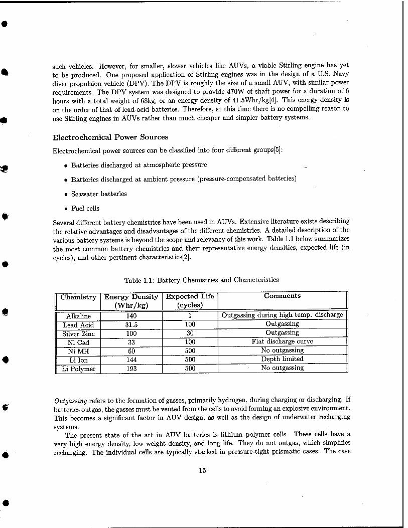
Several different battery chemistries have been used in AUVs. Extensive hterature exists describing the relative advantages and disadvantages of the different chemistries. A detailed description of the various battery systems is beyond the scope and relevancy of this work. Table 1.1 below summarizes the most common battery chemistries and their representative energy densities, expected life (in cycles), and other pertinent characteristics[2].
Table 1.1: Battery Chemistries and Characteristics
Chemistry Energy Density (VV^hr/kg)
Expected Life (cycles)
Comments
Alkaline 140 1 Outgassing during high temp, discharge
Lead Acid 31.5 100 Outgassing
Silver Zinc 100 30 Outgassing
NiCad 33 100 Flat discharge curve NiMH 60 500 No outgassing Li Ion 144 500 Depth hmited
Li Polymer 193 500 No outgassing
Outgassing refers to the formation of gasses, primarily hydrogen, during charging or discharging. If batteries outgas, the gasses must be vented from the cells to avoid forming an explosive environment. This becomes a significant factor in AUV design, as well as the design of underwater recharging systems.
The present state of the art in AUV batteries is lithium polymer cells. These cells have a very high energy density, low weight density, and long life. They do not outgas, which simplifies recharging. The individual cells are typically stacked in pressure-tight prismatic cases. The case
15
can withstand ambient sea pressure, allowing the batteries to be placed outside the pressure hull ofthe AUV[2].
Seawater Batteries
Seawater batteries use seawater as the electrolyte. Thus, seawater batteries have a much higher energy density than other battery types because the electrolyte is not included in the mass of the battery. Seawater batteries have been used in experimental torpedoes and small AUVs. The most common seawater battery chemistries are Mg/AgCl and Mg/02, with energy densities of 200 Whr/kg and 600 Whr/kg, respectively[5]. The drawback of seawater batteries is a very low power output density. For example, a commercially available battery produced by Kongsberg Simrad weighs 120 kg and produces only 2 watts of power, for a power density of 16.7 mW/kg. By comparison, a typical 1 kWh Hthium polymer battery weighs 15 kg and can produce up to 300 watts, for a power density of 20 W/kg. Using a forced flow of seawater increases power output slightly, but it still remains significantly below other battery types. Seawater batteries may find a niche market in very small, very long-endurance AUVs, such as miniature mobile sensors. However, the power limitations prevent seawater batteries from being a significant factor in the mainstream AUV market.
Semi-fuel Cells
A semi-fuel cell is a cell that uses a solid anode and a gaseous cathode^ The most common semi-fuel cells use aluminum as the anode and oxygen as the cathode. Energy is released by a chemical reaction between the aluminum and oxygen in an alkaline electrolyte. Power level can be controlled by varying the concentration of oxygen in the electrolyte. Semi-fuel cells can operate at ambient pressure, with performance independent of depth[7]. Operational semi-fuel cell systems have achieved energy densities of around 100 Whr/kg[5].
Semi-fuel cells are not recharged in the conventional sense. The chemical reaction consumes the aluminum anode and oxygen and produces aluminum hydroxide precipitate; thus, recharging consists of mechanically replacing the anode, changing the electrolyte, and refilling the oxygen supply. This method is much faster than most electrical battery recharging processes, but it requires significant support facilities to store fresh anodes, oxygen, and electrolyte. An additional consideration is the need to dispose ofthe spent electrolyte [7].
Aluminum-air semi-fuel cells have been successfully used for many land-based applications, where the surrounding atmosphere serves as the oxygen source. Two options exist for providing oxygen in underwater applications: carry compressed gaseous oxygen, or carry oxygen in a com- pound that is easily decomposed to liberate oxygen. Both methods have been used successfully in AUVs. The XP-21 AUV, built by Applied Remote Technology, carries gaseous high-pressure (4000 psig) oxygen in two stainless steel spheres [6]. The well-known HUGIN family of AUVs uses semi-fuel cells with hydrogen peroxide (H2O2) as the oxygen source[8].
The HUGIN AUVs, built by Kongsberg Simrad of Norway, are designed for deep sea survey operations. The HUGIN I, built in 1995, used NiCad batteries as a power source. The HUGIN II, operational in 1998, transitioned to the AI-H2O2 semi-fuel cells to extend vehicle endm-ance. The latest version, HUGIN 3000, became operational in 2000 and uses a larger version of the AI-H2O2
^Batteries have solid anodes and cathodes. Fuel cells have gaseous anodes and cathodes[6].
16
semi-fuel cells [5]. HUGIN 3000 is one of the leading commercial AUVs in service today, and is discussed more fully in section 2.2. The HUGIN 3000 operates at a nominal power load of 900W[5]. The semi-fuel cell power source provides 40kWh, sufficient for 40-50 hours of operation[7]. Recharge operations typically take about two hours [8].
The HUGIN AUVs use H2O2 rather than compressed oxygen for several reasons. First, H2O2 can be stored in plastic bags at ambient pressure rather than in stainless steel pressure vessels. The HUGIN systems use a simple metering pump to control the flow of H2O2 into the electrolyte. Second, gaseous oxygen is susceptible to pressure changes with depth, while liquid H2O2 is not. Finally, Uquid H2O2 is much easier to handle than gaseous oxygen during recharge operations [8].
Fuel Cells
Fuel cells have been considered for underwater appUcations for several years. Fuel cells use a chemical reaction between hydrogen and oxygen to release energy in the form of DC electricity. Several types of fuel cells exist, including Proton Exchange Membrane Fuel Cells (PEMFC), Solid Oxide Fuel Cell (SOFC), and Solid Polymer Fuel Cells (SPFC). Underwater applications typically use the SPFC type because of their smaller size and relatively robust design and reliability [9]. A more detailed description of fuel cells can be found in [10].
A major problem with using fuel cells underwater is storage of the reactants. As in semi-fuel cells, the reactants are carried either as compressed gasses, or as compounds that decompose or react to liberate the gas. A third option is to carry the reactants as liquids, but this requires cryogenic systems that are impractical for most AUVs. Compressed gas storage requires large pressure vessels and creates an explosive hazard if not handled properly. On the other hand, storage as a compound is less efficient, because only a fraction of the stored compound is converted to hydrogen or oxygen. Additionally, most storage compounds are highly reactive and require special storage precautions. Typical compounds used are boron hydride to produce hydrogen, and hydrogen peroxide to produce oxygen [5].
The energy density of fuel cells, based solely on weight of reactants, is approximately 2000Whr/kg. However, in order to make a fair comparison with other power sources, the energy density of the entire fuel cell system must be calculated. A complete system sized for a typical AUV and using compressed gas storage spheres would have an energy density of about 130Whr/kg[5]. The energy density of fuel cell systems increases with size, since a larger percentage of total weight can be dedicated to reactants. This is one important reason behind the lag in development of small-scale AUV fuel cell systems.
Fuel cells have been used successfully in several manned submarine designs. The German Class 212 submarines feature nine PEMFC modules capable of producing 34kW each. The Class 214 submarines feature two 120kW PEMFC modules with roughly the same size and weight as the 34kW modules. The fuel cells for both submarine classes are built by Siemens, and use metal hydride and liquid oxygen as reactants [11].
Despite the obvious benefits of fuel cells, only one AUV has successfully operated with a fuel cell power source and been reported in the hterature. The AUV Urashima, developed by the Japan Marine Science and Technology Center (JAMSTEC) for deep-sea exploration, conducted successful sea trials in August 2003. The Urashima is 10m long and weighs approximately 10 tons. Its power source is a 4kW SPFC, using metal hydride and high-pressure gaseous oxygen as reactants[12]. To date, no smaller AUV fuel cell systems have been reported.
17

1.2.2 Near-term Future Predictions
The purpose of this analysis is to attempt to predict the state of AUV power source technology in the near future (five years), as this will dictate the demand (or lack of demand) for a battery recharge system. Based on the information presented above, the following conclusions are reached:
• Lead-acid, alkaline, and hthium polymer batteries will continue to be the most widely used AUV power sources.
• Seawater batteries and semi-fuel cells will have niche markets, but will not appeal to the mainstream AUV market.
• Fuel cells remain too costly and complicated to see widespread proliferation in the market.
These conclusions are justified below. Most AUVs in service today conduct operations on the order of a few hours in duration. The
power demands for missions of this duration can be easily supplied by lead-acid, alkaline, or lithium polymer batteries. Most AUV users do not find it necessary or cost-effective to invest in emerging technologies like fuel cells. The argument can be made that the current operational profile is driven by the available power sources, and that if higher-endurance power sources were available users would change their operations. However, the fact remains that most AUV missions today can be accomplished using conventional battery power sources.
Seawater batteries simply cannot provide the levels of power required by most AUVs. Adding more sensors, communication systems, manipulator arms, etc. to future AUVs will further increase the power demands, making seawater batteries even less viable as time goes on. Semi-fuel cells have energy densities lower than alkaline or lithium polymer batteries (lOOWhr/kg compared to 140Whr/kg and 193Whr/kg, respectively), but significantly higher cost and complexity. The one advantage of semi-fuel cells, the rapid recharge time, is not deemed to be compelhng enough to encourage their use. Furthermore, semi-fuel cell use requires a shift away from conventional recharging methods.
Despite advances being made in the automotive and power generation industries, fuel cells are still considered risky technology. This tends to increase the discount rate used by companies to calculate the value of a potential investment. The effect of the higher discount rates is to make fuel cell projects appear less financially attractive than alternative, more conventional projects. Additionally, higher discount rates imply a higher cost of investment capital; thus, capital-intensive fuel cell projects appear even more expensive than alter natives [13]. The result of this twofold effect is that only very large organizations, like governments and possibly multi-national corporations who operate large numbers of AUVs, will venture into the fuel cell arena. The general trend in AUV use is exactly the opposite, tending towards many small operators running a few AUVs. Thus, fuel cells will continue to lag behind conventional batteries for the near future in the mainstream AUV market.
1.2.3 Motivation for a Battery Recharge System
The above arguments indicate that batteries (lead-acid, alkaHne, or lithium polymer) will continue to be the AUV power source of choice for the near future. However, there are advantages to be
18
gained by extending AUV endurance^, as discussed in section 1.1. Therefore, it is worthwhile to invest in development of an underwater battery recharging system. The remainder of this work describes such a system and evaluates its technical and economic feasibility.
1.3 Previous Docking and Recharge Systems A literature search was conducted to identify previous efforts in the area of AUV docking. A number of AUV docking and recharge systems have been designed and built. The following systems and descriptions are representative of the current state of the art in docking and recharge systems.
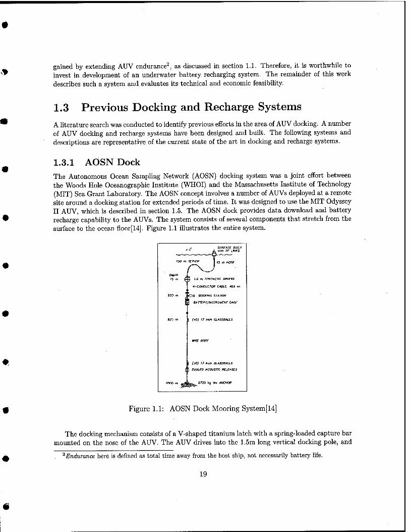
1.3.1 AOSN Dock The Autonomous Ocean Samphng Network (AOSN) docking system was a joint effort between the Woods Hole Oceanographic Institute (WHOI) and the Massachusetts Institute of Technology (MIT) Sea Grant Laboratory. The AOSN concept involves a number of AUVs deployed at a remote site around a docking station for extended periods of time. It was designed to use the MIT Odyssey II AUV, which is described in section 1.5. The AOSN dock provides data download and battery recharge capabihty to the AUVs. The system consists of several components that stretch from the surface to the ocean floor [14]. Figure 1.1 illustrates the entire system.
susrAor Boor
iM rn rcmm 1,5 „ HOSE
0«i»i i fi m ^ 1.6 m SWTACnc SPHCRE
4-CONDilCroK CABLE, 42i m
500 m %
!=a oocKma STA new
J BAmPY/lNSKUUrNT CAGf \
S?2 m 1 (40) 17 *icfi CL/kSSaMLS
WSE RCpr
1 (X) 1' hcJ. aASSSilLS
( ] BMLtO ACOUSTIC KEiEASCS
.!500 m .^ L^2730 tj Wrt AiNaiOK
Figure 1.1: AOSN Dock Mooring System [14]
The docking mechanism consists of a V-shaped titanium latch with a spring-loaded capture bar mounted on the nose of the AUV. The AUV drives into the 1.5m long vertical docking pole, and
'^Endurance here is defined as total time away from the host ship, not necessarily battery life.
19
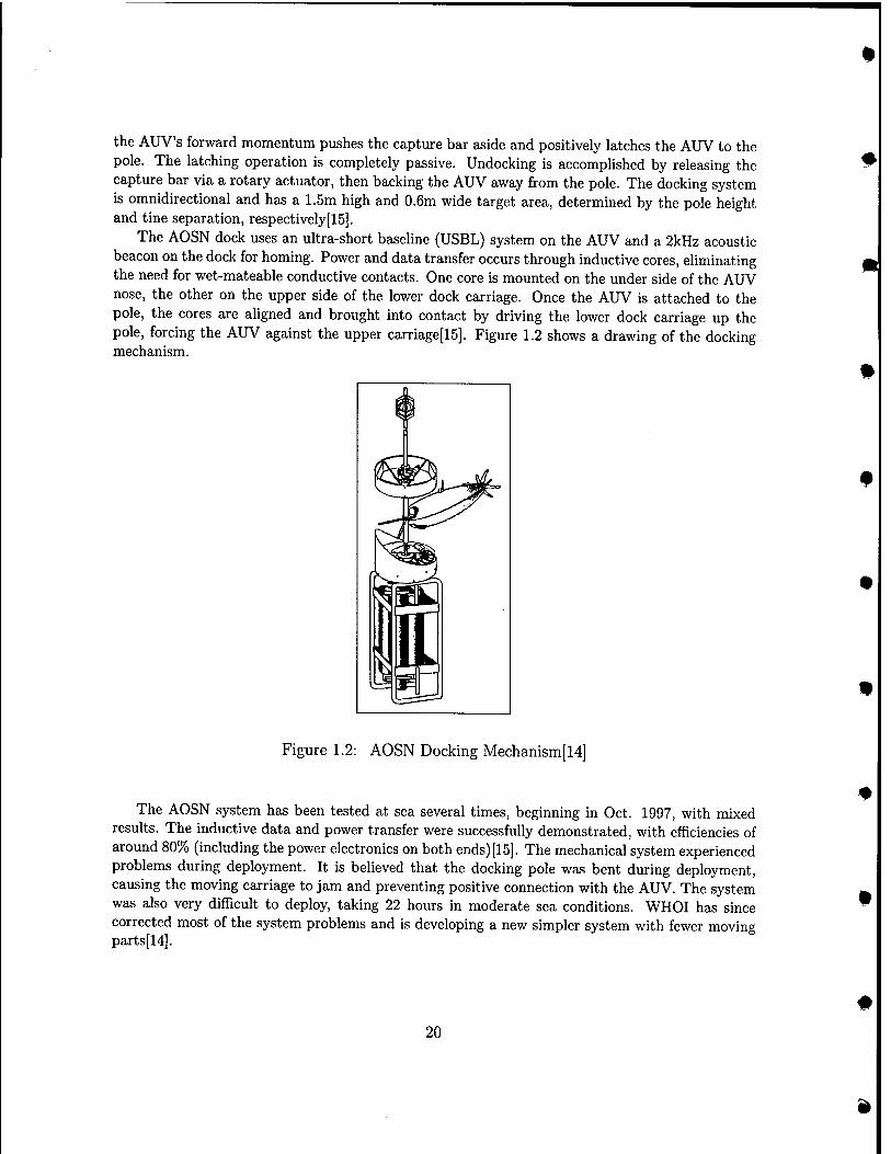
the AUV's forward momentum pushes the capture bar aside and positively latches the AUV to the pole. The latching operation is completely passive. Undocking is accomplished by releasing the capture bar via a rotary actuator, then backing the AUV away from the pole. The docking system is omnidirectional and has a 1.5m high and 0.6m wide target area, determined by the pole height and tine separation, respectively[15].
The AOSN dock uses an ultra-short baseline (USBL) system on the AUV and a 2kHz acoustic beacon on the dock for homing. Power and data transfer occurs through inductive cores, eliminating the need for wet-mateable conductive contacts. One core is mounted on the under side of the AUV nose, the other on the upper side of the lower dock carriage. Once the AUV is attached to the pole, the cores are aligned and brought into contact by driving the lower dock carriage up the pole, forcing the AUV against the upper carriage[15]. Figure 1.2 shows a drawing of the docking mechanism.
Figure 1.2: AOSN Docking Mechanism[14]
The AOSN system has been tested at sea several times, beginning in Oct. 1997, with mixed results. The inductive data and power transfer were successfully demonstrated, with efficiencies of around 80% (including the power electronics on both ends) [15]. The mechanical system experienced problems during deployment. It is believed that the docking pole was bent during deployment, causing the moving carriage to jam and preventing positive connection with the AUV. The system was also very difficult to deploy, taking 22 hours in moderate sea conditions. WHOI has since corrected most of the system problems and is developing a new simpler system with fewer moving parts [14].
20
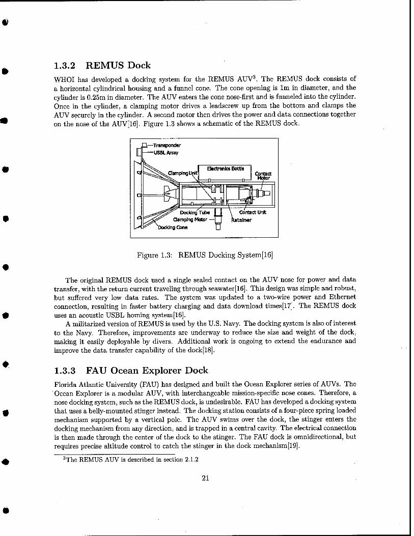
1.3.2 REMUS Dock WHOI has developed a docking system for the REMUS AUV^. The REMUS dock consists of a horizontal cyhndrical housing and a funnel cone. The cone opening is Im in diameter, and the cylinder is 0.25m in diameter. The AUV enters the cone nose-first and is funneled into the cylinder. Once in the cyHnder, a clamping motor drives a leadscrew up from the bottom and clamps the AUV securely in the cylinder. A second motor then drives the power and data connections together on the nose of the AUrV[16]. Figure 1.3 shows a schematic of the REMUS dock.
jP.—^Transponder
—USBL Array
Clamping Unit
Docking Tube Qamping i^otx>r
Oocldng Cone
Figure 1.3: REMUS Docking System[16]
The original REMUS dock used a single sealed contact on the AUV nose for power and data transfer, with the return current travehng through seawater[16]. This design was simple and robust, but suffered very low data rates. The system was updated to a two-wire power and Ethernet connection, resulting in faster battery charging and data download times[17]. The REMUS dock uses an acoustic USBL homing system[16].
A militarized version of REMUS is used by the U.S. Navy. The docking system is also of interest to the Navy. Therefore, improvements are underway to reduce the size and weight of the dock, making it easily deployable by divers. Additional work is ongoing to extend the endurance and improve the data transfer capability of the dock[18].
1.3.3 FAU Ocean Explorer Dock Florida Atlantic University (FAU) has designed and built the Ocean Explorer series of AUVs. The Ocean Explorer is a modular AUV, with interchangeable mission-specific nose cones. Therefore, a nose docking system, such as the REMUS dock, is undesirable. FAU has developed a docking system that uses a belly-mounted stinger instead. The docking station consists of a fomr-piece spring loaded mechanism supported by a vertical pole. The AUV swims over the dock, the stinger enters the docking mechanism from any direction, and is trapped in a central cavity. The electrical connection is then made through the center of the dock to the stinger. The FAU dock is omnidirectional, but requires precise altitude control to catch the stinger in the dock mechanism [19].
^The REMUS AUV is described in section 2.1.2
21
1.3.4 Flying Plug Socket
The Flying Plug AUV (described in section 2.1.2) uses a docking system very similar to the REMUS dock. The Flying Plug dock is referred to as the Socket. It uses a cone and cylinder system to capture the AUV and align the power and data connections. A unique feature of the Socket is the use of a combination acoustic/optical homing scheme. An acoustic beacon is used to get the AUV close to the dock (i.e., within a few meters), then an optical tracking system is used for final alignment and approach. The optical tracking system is similar to those used by laser-guided munitions. The Socket also uses optical data transfer, rather than conductive or inductive electrical couplings [20].
1.3.5 Eurodocker
Eurodocker is a project funded by the European Commission, DG XII, under the Marine Science and Technology program (MAST). The goal of the project is to develop a universal garage-type docking station that can be used by a variety of AUVs. A prototype has been built and successfully tested using Maridan's Martin AUV. The dock consists of a tubular frame box structure that completely encloses the AUV, providing physical protection while docked. An active shock absorption system using water bags absorbs the impact of the docking AUV. A variable buoyancy system allows precise depth positioning of the dock. Power and data transfer is via wet-mateable pin connections. Two Eurodocker configurations are envisioned, one towed by a support ship and the other permanently deployed on the ocean floor. The Eurodocker project represents one of the first efforts to create a universal dock for use by commercial work-class (as opposed to research or military) AUVs[19].
1.3.6 U.S. Navy Torpedo Tube Launch and Recovery System
The Navy's Torpedo Tube Launch and Recovery (TTLR) system is being developed to launch and recover AUVs from a submerged submarine. While not a true docking system in terms of battery recharge and data transfer, the TTLR system illustrates the use of an articulated arm to physically capture and retrieve an AUV. The arm deploys from the upper torpedo tube and extends an aft- facing receiver cone. The AUV approaches on a course parallel to the submarine, using acoustic homing. A retractable probe on the AUV nose is driven into the receiver cone. A support ring then grabs the mid-body of the AUV, creating a secure two-point connection. The arm maneuvers and forces the AUV into the lower torpedo tube, tail-first. The arm is then retracted into the upper tube and both tube shutter doors are closed[21]. The TTLR system is being developed by NUWC and built by Boeing. A prototype system has been built and installed on a barge, and testing is ongoing. The timeframe for installation on a submarine is unclear, dependent on the prototype results[21].
1.4 Overview of Proposed System and Design Goals The primary goal of the design phase of this work was to develop a docking and recharge system compatible with all present and near-term future U.S. Navy AUVs. A secondary goal was to extend the compatibility of the system to the commercial AUV market. A major factor distinguishing the present work from previous systems (with the exception of Eurodocker) is the attempt to make
22
the system universally compatible with a range of AUVs. It was decided early in the project that the docking system would only provide battery recharge power, and not data interface capability. Ongoing advances in optical and acoustic data transfer techniques, along with the growing need for real-time data, will soon make periodic data dumping techniques obsolete.
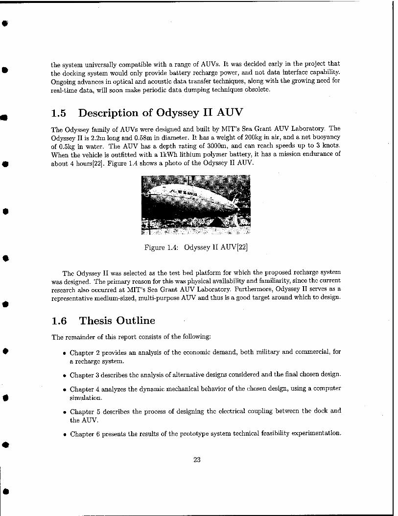
1.5 Description of Odyssey II AUV The Odyssey family of AUVs were designed and built by MIT's Sea Grant AUV Laboratory. The Odyssey II is 2.2m long and 0.58m in diameter. It has a weight of 200kg in air, and a net buoyancy of 0.5kg in water. The AUV has a depth rating of 3000m, and can reach speeds up to 3 knots. When the vehicle is outfitted with a IkWh lithium polymer battery, it has a mission endurance of about 4 hours[22]. Figure 1.4 shows a photo of the Odyssey II AUV.
Figure 1.4: Odyssey II AUV[22]
The Odyssey II was selected as the test bed platform for which the proposed recharge system was designed. The primary reason for this was physical availabiUty and familiarity, since the current research also occurred at MIT's Sea Grant AUV Laboratory. Furthermore, Odyssey II serves as a representative medium-sized, multi-purpose AUV and thus is a good target around which to design.
1.6 Thesis Outline The remainder of this report consists of the following:
•
•
•
Chapter 2 provides an analysis of the economic demand, both miUtary and commercial, for a recharge system.
Chapter 3 describes the analysis of alternative designs considered and the final chosen design.
Chapter 4 analyzes the dynamic mechanical behavior of the chosen design, using a computer simulation.
Chapter 5 describes the process of designing the electrical couphng between the dock and the AUV.
Chapter 6 presents the results of the prototype system technical feasibility experimentation.
23

• Chapter 7 describes the mechanical design of the latch interface between the dock and the AUV.
• Chapter 8 assesses the economic feasibility of the proposed system for both military and commercial markets.
• Chapter 9 summarizes conclusions from the present work and identifies required future work.
24
Chapter 2
Demand for an AUV Recharge System
2.1 Military Market The United States Navy is one of the leading users of AUVs in the world. Furthermore, the Navy has plans to greatly expand its use of AUVs in the near future [23]. Navy acquisition funding for AUV programs more than doubled from FY02 to FY03[24]. As such, the U.S. Navy is the primary target market for an AUV battery recharge system.
2.1.1 Roles for Navy AUVs AUVs have the potential to perform four broad military roles: maritime reconnaissance, under- sea search and survey, communications and navigation, and submarine tracking[25]. Each role is described in detail below.
Metritime Reconnaissance
The number one mission priority for AUV application by the U.S. Navy is Maritime Reconnaissance [23]. AUVs are capable of performing a number of reconnaissance tasks currently performed by manned platforms such as submarines or aircraft. The main advantage of AUVs in recormaissance missions is increased stealth. AUVs could be covertly deployed into areas that are inaccessible to submarines or aircraft, such as poUtically denied areas or extremely shallow water. An AUV could operate undetected in these areas for long periods of time, gathering valuable information in the process. Three main reconnaissance uses of AUVs are intelligence, surveillance, and reconnaissance (ISR); battle damage assessment (BDA); and remote target designation [25]^.
ISR is a ready-made mission for an AUV. AUVs are capable of gathering visual, electromagnetic, or acoustic data. This data can be relayed near real-time back to a manned platform, or it can be stored onboard the AUV until it returns to the host platform. It is understood that stealth is compromised during communication. In essence, the AUV would operate as a set of remote eyes and ears for the host platform.
^A complete list of all nomenclature and acronyms used in chapter 2 is located in section 2.3.
25
BDA is an increasingly important mission in this era of limited, precision warfare. Presently, satellite or aircraft photography is relied upon for most BDA. AUVs could perform this mission with greater stealth and potentially greater accuracy. However, AUVs could only perform BDA on ship or coastal land targets, since visual contact would be required.
The third potential reconnaissance mission of AUVs is remote target designation. AUVs could be equipped with laser target designators and used to identify targets for cruise missile or aircraft attacks. However, as with BDA, this role would be limited to ship or coastal targets.
Undersea Search and Survey
The oldest and most highly developed military application of AUVs is Undersea Search and Survey. The primary advantage of AUVs over alternative platforms in this mission area is the AUVs ability to operate in regions or environments inaccessible to manned vehicles. A secondary advantage of AUVs is that they can often perform a search or survey mission more economically than a manned vehicle. Three main search and survey applications of AUVs are mine countermeasures, salvage, and hydrographic survey [25].
Mine countermeasures (MCM) was the first military application of AUVs [25]. The appeal of using unmanned vehicles to detect and detonate mines is readily apparent. Minefields can be safely cleared without needlessly risking human life. Additionally, AUV systems can clear mines faster and more efficiently than human operators. Finally, an AUV MCM system could have the added advantage of stealth if deployed from a submarine. Thus, a minefield could conceivably be neutralized without the opponent realizing it.
Underwater military salvage is another area in which AUVs could have a significant impact. AUVs could be made capable of performing all aspects of a salvage operation, from initial detection to photography and videotaping to actual retrieval of objects. AUVs are more advantageous than human divers because they can operate at deeper depths and remain on station longer. Additionally, AUVs can safely operate in salvage sites that may be contaminated by hazardous materials or nuclear radiation[25].
The third potential search and survey mission of AUVs is hydrographic and oceanographic sur- vey. This mission covers a wide range of activities, including but not limited to bottom surveys for the purpose of charting, plotting of ocean currents, weather observation, and survey of amphibious landing zones. Clearly some of these activities are not strictly military in nature and overlap with commercial applications of AUVs.
Communication and Navigation
The communication and navigation role is a key component of the other AUV missions in addition to being a stand-alone role. An essential part of any AUV mission is the ability to communicate the information collected back to the host platform. An AUV must also be able to navigate and know its position with great precision to accomphsh most missions. As for stand-alone communica- tion/navigation missions, AUVs could potentially function as mobile communication relay stations or as a backup to satellite systems [25].
An AUV could function as a communication relay simply by positioning itself midway between two communications stations, within line of sight (LOS) of each. The AUV would surface, or extend an antenna mast above the surface. Communications could then be conducted using less detectable LOS transmissions rather than satellite transmissions. An AUV could also act as a
26
#
submerged acoustic relay station. Additionally, AUVs could be used as mobile satellite relay stations (again requiring the AUV to be on or near the surface), creating an additional hnk in the chain between transmitter and receiver. The purpose of this would be to make it more difficult to triangulate the location of a transmission source. This role could be extremely useful in submarine communications, where remaining undetected is a priority.
A group of AUVs could also potentially be organized into an underwater, mobile communica- tions/navigation network. Such a system could be vital in case of a Global Positioning System (GPS) failure or jamming by a hostile force[25]. This system would, however, be very limited in range due to underwater acoustic limitations.
Submarine Tracking and Trailing
Submarine tracking and traihng is the most visionary of the potential AUV appUcations and the one requiring the most technological developments to reach fruition. The ultimate goal of this application is to create a fully autonomous system capable of detecting a submarine and tracking it for extended periods of time over long distances of open ocean[25]. This capability would supple- ment the activities of manned submarines, thereby freeing them to perform other tasks. This goal will be very difficult to fully achieve. To put it in perspective, today this mission is chaUenging even for a billion doUar nuclear submarine manned with 120 men. Attempting to perform the same mission with an affordable unmanned system is a monumental undertaking and wiU require extensive long-term planning and investment.
In the shorter term, AUVs could perform some limited portions of the anti-submarine warfare (ASW) mission. One such mission would be to function as a mobile sonar platform for initial detection of opposing submarines [25]. The AUVs would function similar to the existing sonar arrays stretched across regions of the ocean floor, but with the added benefit of mobility. An AUV sonar platform would have an advantage over a manned submarine in that the AUV is much smaller and potentially quieter, due to less machinery noise. Therefore, the AUV could detect an opposing submarine earlier due to less own-noise interference, and would also be less likely to be counter-detected by the opponent.
Several major obstacles stand in the way of creating AUVs to perform this mission. First, speed limitations on existing AUVs would severely limit their ability to track a high-speed nuclear submarine. Second, existing ASW sonar systems are too large to be mounted on an AUV. Third, the necessary communications links do not currently exist. However, many experts beUeve all these obstacles can be overcome and a fully autonomous submarine tracking system will someday be developed [25].
2.1.2 Summary of Navy AUV Programs The Navy's development and use of AUVs is guided by The Navy Unmanned Undersea Vehicle (UUV) Master Plan [2Z]^. Implementation of the plan is carried out by the Naval Sea Systems Command (NAVSEA), PMS403. Several research AUV programs, one of which is the MIT Odyssey described in section 1.5, are sponsored by the Office of Naval Research (ONR). Development of Navy AUV programs is done primarily by the Naval Undersea Warfare Center (NUWC) and the
2The Navy term UUV is synonymous with the generally-accepted term AUV, and the two are used interchangeably in this paper.
27
Space and Naval Warfare Systems Center (SPAWAR). The Navy currently has several tactical AUV systems either operational or in development for near-term deployment. Several other systems and concepts are being considered for long-term use. The systems are described below, starting with the most mature first.
REMUS/SAHRV
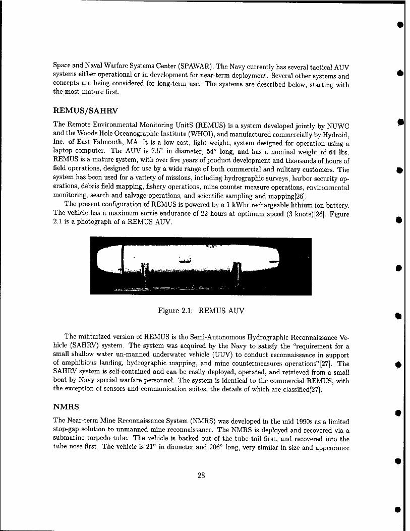
The Remote Environmental Monitoring UnitS (REMUS) is a system developed jointly by NUWC and the Woods Hole Oceanographic Institute (WHOI), and manufactured commercially by Hydroid, Inc. of East Falmouth, MA. It is a low cost, hght weight, system designed for operation using a laptop computer. The AUV is 7.5" in diameter, 54" long, and has a nominal weight of 64 lbs. REMUS is a mature system, with over five years of product development and thousands of hours of field operations, designed for use by a wide range of both commercial and military customers. The system has been used for a variety of missions, including hydrographic surveys, harbor security op- erations, debris field mapping, fishery operations, mine counter measure operations, environmental monitoring, search and salvage operations, and scientific sampling and mapping[26].
The present configuration of REMUS is powered by a 1 kWhr rechargeable lithium ion battery. The vehicle has a maximum sortie endurance of 22 hours at optimum speed (3 knots) [26]. Figure 2.1 is a photograph of a REMUS AUV.
Figure 2.1: REMUS AUV
The militarized version of REMUS is the Semi-Autonomous Hydrographic Reconnaissance Ve- hicle (SAHRV) system. The system was acquired by the Navy to satisfy the "requirement for a small shallow water un-manned underwater vehicle (UUV) to conduct reconnaissance in support of amphibious landing, hydrographic mapping, and mine countermeasiures operations" [27]. The SAHRV system is self-contained and can be easily deployed, operated, and retrieved firom a small boat by Navy special warfare personnel. The system is identical to the commercial REMUS, with the exception of sensors and communication suites, the details of which are classified[27].
NMRS
The Near-term Mine Reconnaissance System (NMRS) was developed in the mid 1990s as a limited stop-gap solution to unmanned mine reconnaissance. The NMRS is deployed and recovered via a submarine torpedo tube. The vehicle is backed out of the tube tail first, and recovered into the tube nose first. The vehicle is 21" in diameter and 206" long, very similar in size and appearance
28
to a Mk48 torpedo. It carries forward-looking and side-looking sonar capable of detecting mine-like objects. The NMRS is powered by rechargeable silver-zinc batteries[28].
The NMRS is not a true AUV, because it normally does not operate autonomously. The vehicle is remotely controlled from the submarine via a fiber optic cable. The vehicle does have a limited autonomous capability to return to the submarine and be recovered in the event the fiber optic cable fails[28].
The NMRS was planned to reach initial operational capability (IOC) in FY98[28]. However, it has never achieved widespread operational use and remains in a fleet contingency status [24]. Despite this fact, the NMRS was an important learning step in the development of the next- generation minehunting system.
Flying Plug
The Flying Plug is a small AUV developed by SPAWAR to function as a connectivity channel. The vehicle is 9" in diameter and 50" long. It is sized so that it can be launched from the trash disposal unit of a submarine. The system is expendable, meaning the vehicle is not recovered to the submarine[20].
The Flying Plug is designed to dock with a remote sensor or information node and transfer data back to the host submarine. The vehicle is tethered to the submarine by a 20 km long fiber optic cable. The cable provides guidance commands to the vehicle and serves as the data link back to the submarine. The cable allows up to 120 Mbit/second of data transfer[20]. A critical element of the system is the docking station described earlier in section 1.3.4.
A potential application of the Flying Plug is to service and retrieve data from a network of remote underwater sensors. Another potential use is the transfer of data or tasking information to the submarine from a shore command via a submarine cable. A long submarine cable would be deployed across the ocean floor, with Flying Plug connection points spaced along its length. The submarine would deploy a Flying Plug to dock with the nearest connection point and retrieve any waiting data or messages [20]. This would eliminate the need for the submarine to periodically come to periscope depth and risk detection.
A major drawback of the Flying Plug system is the lack of real-time data retrieval. Unless the submarine is continuously tethered to the remote node, there wiU always be an inherent time lag. As underwater acoustic communications continue to improve in speed, range, and bandwidth, the utiUty of the Flying Plug system will most likely fade away.
LMRS (AN/BLQ-11)
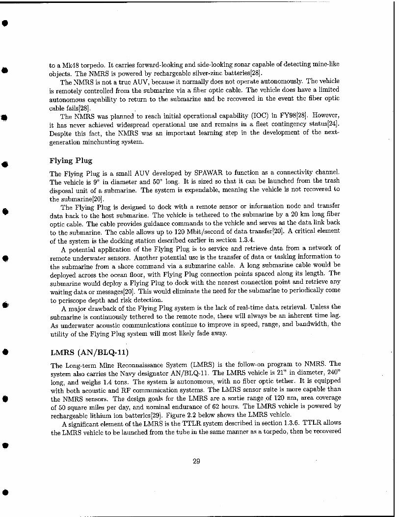
The Long-term Mine Reconnaissance System (LMRS) is the follow-on program to NMRS. The system also carries the Navy designator AN/BLQ-11. The LMRS vehicle is 21" in diameter, 240" long, and weighs 1.4 tons. The system is autonomous, with no fiber optic tether. It is equipped with both acoustic and RF communication systems. The LMRS sensor suite is more capable than the NMRS sensors. The design goals for the LMRS are a sortie range of 120 nm, area coverage of 50 square miles per day, and nominal endurance of 62 hours. The LMRS vehicle is powered by rechargeable lithium ion batteries[29]. Figure 2.2 below shows the LMRS vehicle.
A significant element of the LMRS is the TTLR system described in section 1.3.6. TTLR allows the LMRS vehicle to be launched from the tube in the same manner as a torpedo, then be recovered
29
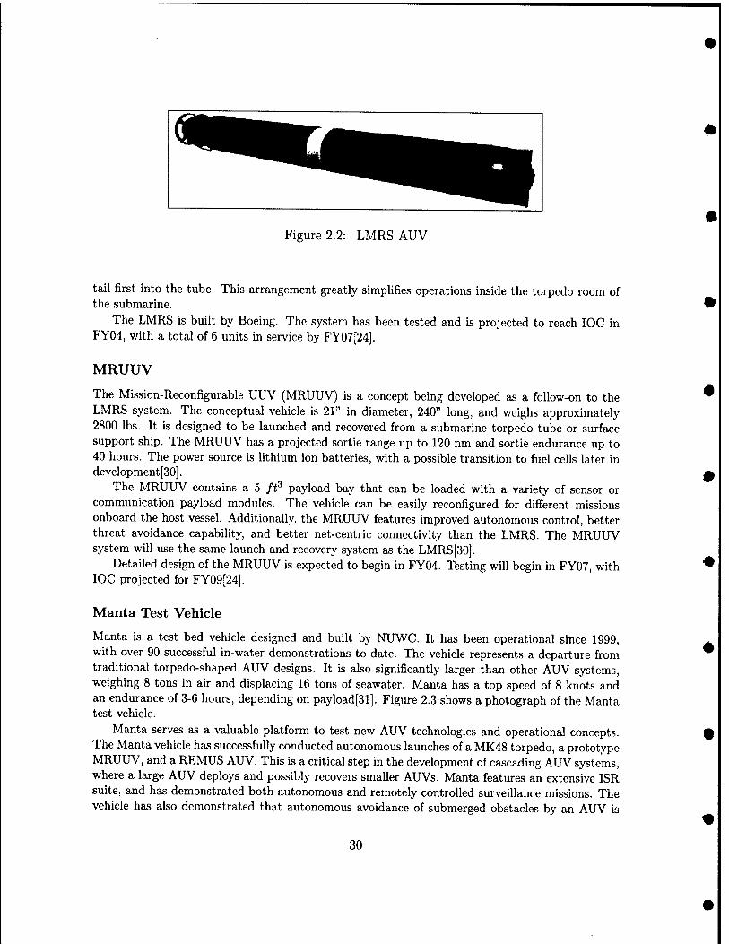
Figure 2.2: LMRS AUV
tail first into the tube. Tiiis arrangement greatly simplifies operations inside the torpedo room of the submarine.
The LMRS is built by Boeing. The system has been tested and is projected to reach IOC in FY04, with a total of 6 units in service by FY07[24].
MRUUV
The Mission-Reconfigurable UUV (MRUUV) is a concept being developed as a follow-on to the LMRS system. The conceptual vehicle is 21" in diameter, 240" long, and weighs approximately 2800 lbs. It is designed to be launched and recovered from a submarine torpedo tube or surface support ship. The MRUUV has a projected sortie range up to 120 nm and sortie endurance up to 40 hours. The power source is lithium ion batteries, with a possible transition to fuel cells later in development [30].
The MRUUV contains a 5 ft^ payload bay that can be loaded with a variety of sensor or communication payload modules. The vehicle can be easily reconfigured for different missions onboard the host vessel. Additionally, the MRUUV features improved autonomous control, better threat avoidance capability, and better net-centric connectivity than the LMRS. The MRUUV system will use the same launch and recovery system as the LMRS [30].
Detailed design of the MRUUV is expected to begin in FY04. Testing will begin in FY07, with IOC projected for FY09[24].
Manta Test Vehicle
Manta is a test bed vehicle designed and built by NUWC. It has been operational since 1999, with over 90 successful in-water demonstrations to date. The vehicle represents a departure from traditional torpedo-shaped AUV designs. It is also significantly larger than other AUV systems, weighing 8 tons in air and displacing 16 tons of seawater. Manta has a top speed of 8 knots and an endurance of 3-6 hours, depending on payload[31]. Figure 2.3 shows a photograph of the Manta test vehicle.
Manta serves as a valuable platform to test new AUV technologies and operational concepts. The Manta vehicle has successfully conducted autonomous launches of a MK48 torpedo, a prototype MRUUV, and a REMUS AUV. This is a critical step in the development of cascading AUV systems, where a large AUV deploys and possibly recovers smaller AUVs. Manta features an extensive ISR suite, and has demonstrated both autonomous and remotely controlled surveillance missions. The vehicle has also demonstrated that autonomous avoidance of submerged obstacles by an AUV is
30
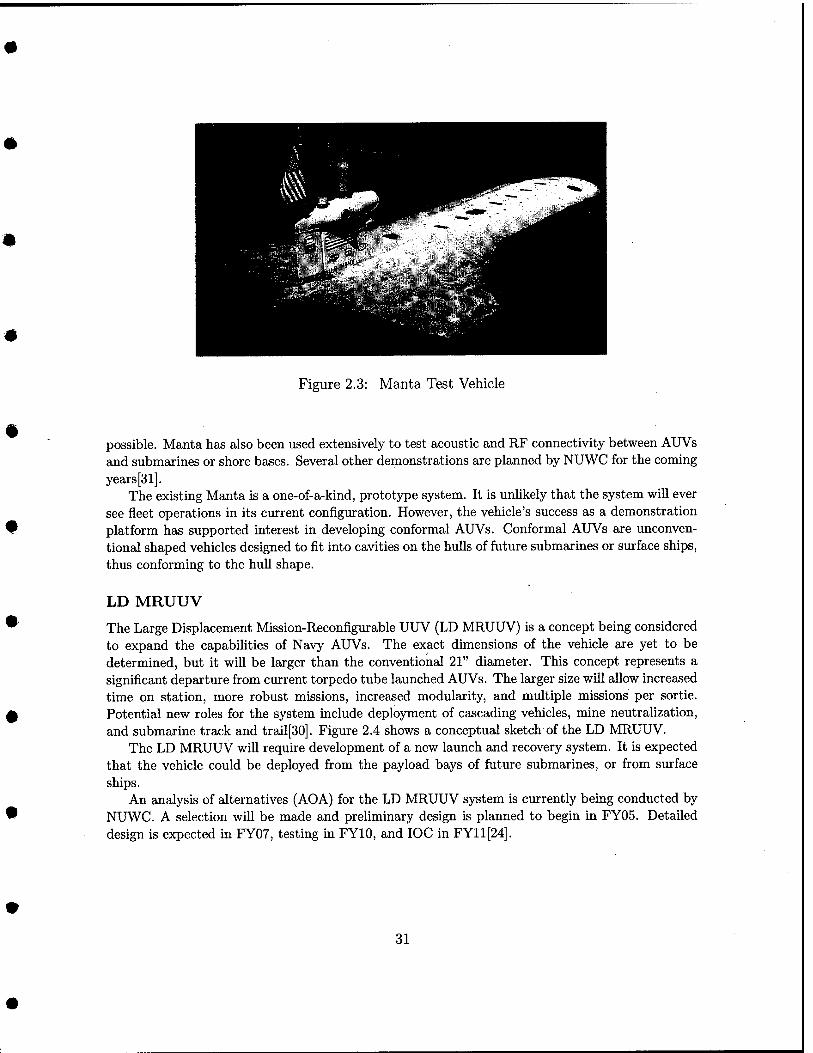
Figure 2.3: Manta Test Vehicle
possible. Manta has also been used extensively to test acoustic and RF connectivity between AUVs and submarines or shore bases. Several other demonstrations are planned by NUWC for the coming years [31].
The existing Manta is a one-of-a-kind, prototype system. It is unlikely that the system will ever see fleet operations in its current configuration. However, the vehicle's success as a demonstration platform has supported interest in developing conformal AUVs. Conformal AUVs are unconven- tional shaped vehicles designed to fit into cavities on the hulls of future submarines or surface ships, thus conforming to the hull shape.
LD MRUUV
The Large Displacement Mission-Reconfigurable UUV (LD MRUUV) is a concept being considered to expand the capabilities of Navy AUVs. The exact dimensions of the vehicle are yet to be determined, but it wiU be larger than the conventional 21" diameter. This concept represents a significant departure from current torpedo tube launched AUVs. The larger size will allow increased time on station, more robust missions, increased modularity, and multiple missions per sortie. Potential new roles for the system include deployment of cascading vehicles, mine neutrahzation, and submarine track and trail[30]. Figure 2.4 shows a conceptual sketch of the LD MRUUV.
The LD MRUUV will require development of a new launch and recovery system. It is expected that the vehicle could be deployed from the payload bays of future submarines, or from surface ships.
An analysis of alternatives (AOA) for the LD MRUUV system is currently being conducted by NUWC. A selection wiU be made and prehminary design is planned to begin in FY05. Detailed design is expected in FY07, testing in FYIO, and IOC in FY11[24].
31
Figure 2.4: LD MRUUV Concept Sketch
2.1.3 Network-centric Warfare Scenario
The U.S. Navy is currently shifting its operational focus from platform-centric warfare to network- centric, or net-centric, warfare. Net-centric warfare utilizes geographically dispersed forces con- nected by a real-time information network. The network links sensors, shooters, and command and control platforms to allow faster decision making and quicker response times. The result is a naval force that can meet objectives more efficiently and with fewer resources than a traditional platform-centric force [32].
The utilization of distributed assets is a key element of net-centric warfare. In particular, un- manned vehicles (UVs) have the potential to greatly enhance the operational effectiveness of manned platforms. Some unmanned systems, such as AUV minehunting systems and unmanned aerial ve- hicle (UAV) surveillance systems, have already proven their worth in combat operations. However, the potential benefits of fully interconnected networks of unmanned vehicles remain largely unreal- ized. Finding an efficient method to recharge UVs on station is a key enabling technology to allow further development of such systems. This research and proposed system provide one solution to the problem of recharging AUVs.
The underlying goal of using UVs in military applications is to expand the coverage and effec- tiveness of manned platforms. UVs can act as a very powerful force multiplier. A Navy platform, such as a minesweeper or a destroyer or a submarine, has a certain level of effectiveness for each mission. For example, a minesweeper's effectiveness at clearing mines depends on its speed, maneu- verability, sensors, and a number of other characteristics. Most of these characteristics are inherent to the ship. It is therefore difficult to improve the operational effectiveness of a ship after it is in service. However, an interconnected network of UVs can be deployed around a manned asset. As- suming seamless near real-time transfer of data between all vehicles (both manned and unmanned), the result is a virtual platform with a much wider area of coverage and greater effectiveness.
Individual UVs can play several different roles in a net-centric warfare scenario. The first and most widely developed role is as a remote sensor platform. UV sensor platforms can penetrate previously denied or unsafe areas and extend the sensor coverage of the force, without exposing manned assets to danger. Second, UVs can serve as communication relay nodes. This role is extremely important underwater, where present acoustic communications technology is very range- hmited. The final role, still largely untapped, is the use of UVs as implementers^. Examples of this role include using AUVs to detonate mines, and using UAVs to fire missiles [33].
^ Implementer here is defined as a platform that takes action against a target based on previously acquired information.
32
To demonstrate the utility of an AUV recharge system, a potential operational scenario is described. The scenario considered here is a Navy surface combatant operating close to a hostile coasthne. The mission may be mine countermeasures, naval gunfire support, or coastal surveillance. The ship is surrounded by a network of AUVs, UAVs, and unmanned surface vehicles (USVs) equipped to contribute to the same mission as the ship. Each AUV is accompanied by a designated USV shadow. The USV remains directly above the AUV at all times and maintains a vertical acoustic communications link between the two vehicles. The USV is equipped with RF or satellite communications to relay the data to the rest of the network. In this way, the problem of near real-time communication with underwater vehicles is solved"*.
The surface combatant engaged in the mission must be able to prosecute the mission while simultaneously defending itself from hostile attack. The current manning and operational envi- ronment of combatants may not allow the ship to also perform the complex task of managing the network of UVs. Furthermore, most current combatants do not have space or weight margins to allow hosting and controlling a UV network. Therefore, a designated UV mother ship will be developed.
The mother ship will remain offshore during the mission, nominally 100 nm from the coast. This places the vessel safely out of range of most shore-based threats. However, because of the long distance between the UV network and the mother ship, and the inherently short endurance of most battery-powered AUV systems, a method of remotely recharging AUVs is required. The proposed system meets this need and extends the endurance of the AUV network. Figure 2.5 below illustrates the operational scenario.
■UJHI' ,pl' I" I ——
rw'f - / - .
l^w*:*" ;'■'. •■ ,-r..ni.t" ■ ."-f-"/..'-^■Vius.-.R.L:?-.
'H^^^v*■■■■*''•'■'-. '- ■ -■ '- ■■■•«-''.'-:-■■.-.■=
■MA ^^^ - f^.fj:!;jxcitttr. .'. ; r ■■■
^K;' >=▼, '
Figure 2.5: Net-Centric Warfare Scenario
■^True real-time communication with submerged AUVs is difRcult to achieve due to the slow data rate and time lag inherent to present acoustic communications.
33
Tanker AUV Concept
The tanker AUV is simply an AUV equipped with a large bank of batteries that transits from the mother ship into the mission area with the UV network. It then sits on the ocean floor and acts as a remote charging station throughout the mission. The individual network AUVs dock with the tanker at prescribed intervals. The system described in the remainder of this paper is the interface between the tanker and the network AUVs. The network endurance is thus limited only by the battery capacity of the tanker. At the conclusion of the mission, the tanker AUV transits back to the mother ship and is recovered. The tanker AUV requires no sensors and only a rudimentary navigation system to perform its task, allowing maximum battery-carrying capability.
A quick analysis using standard submarine and AUV design methods was conducted to deter- mine the approximate required size of a tanker AUV. The theoretical tanker is capable of supporting a network of 5 Odyssey II AUVs for a period of 5 days, or a total of 25 AUV-days. Based on his- torical data for Odyssey II, 1 AUV-day is assumed to consume 6 kW-hours of energy. Other assumptions and the resulting dimensions of the tanker AUV are summarized in table 2.1 below.
Table 2.1: Conceptual Tanker AUV Design
Assumptions Endurance = 25 AUV-days 1 AUV-day = 6 kW-hours Transit range = 100 nm Transit speed = 4 knots
Loiter time = 5 days Charging efficiency = 85%
Loiter power consumption^ = 25 W Battery type = Lithium ion
Battery volume = 0.334 ft^kW-hour Battery weight = 33 Ib/kW-hour
Tanker Dimensions Length = 25 ft
Diameter = 2.5 ft
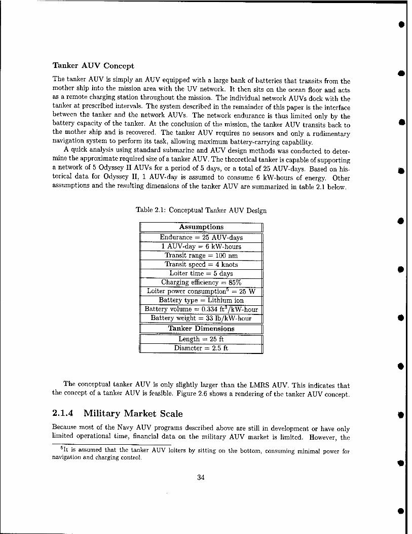
The conceptual tanker AUV is only slightly larger than the LMRS AUV. This indicates that the concept of a tanker AUV is feasible. Figure 2.6 shows a rendering of the tanker AUV concept.
2.1.4 Military Market Scale
Because most of the Navy AUV programs described above are still in development or have only limited operational time, financial data on the military AUV market is limited. However, the
^It is assumed that the tanker AUV loiters by sitting on the bottom, consuming minimal power for navigation and charging control.
34
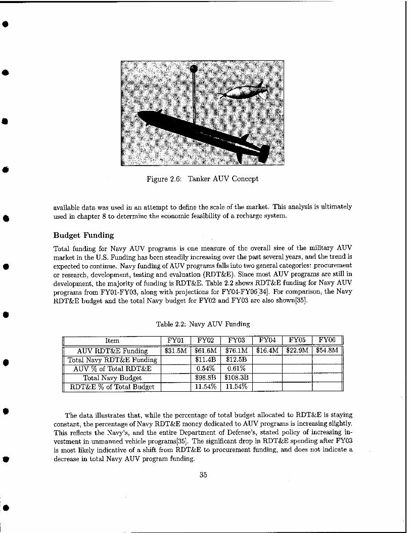
Figure 2.6: Tanker AUV Concept
available data was used in an attempt to define the scale of the market. This analysis is ultimately used in chapter 8 to determine the economic feasibility of a recharge system.
Budget Funding
Total funding for Navy AUV programs is one measure of the overall size of the mihtary AUV market in the U.S. Funding has been steadily increasing over the past several years, and the trend is expected to continue. Navy funding of AUV programs falls into two general categories: procurement or research, development, testing and evaluation (RDT&E). Since most AUV programs are still in development, the majority of funding is RDT&E. Table 2.2 shows RDT&E funding for Navy AUV programs from FY01-FY03, along with projections for FY04-FY06[34]. For comparison, the Navy RDT&E budget and the total Navy budget for FY02 and FY03 are also shown [35].
Table 2.2: Navy AUV Funding
Item FYOl FY02 FY03 FY04 FY05 FY06
AUV RDT&E Funding $31.5M $61.6M $76.1M $16.4M $22.9M $54.8M Total Navy RDT&E Funding $11.4B $12.5B
AUV % of Total RDT&E 0.54% 0.61% Total Navy Budget $98.8B $108.3B
RDT&E % of Total Budget 11.54% 11.54%
The data illustrates that, while the percentage of total budget allocated to RDT&E is staying constant, the percentage of Navy RDT&E money dedicated to AUV programs is increasing shghtly. This reflects the Navy's, and the entire Department of Defense's, stated policy of increasing in- vestment in unmanned vehicle programs [35]. The significant drop in RDT&E spending after FY03 is most likely indicative of a shift from RDT&E to procurement funding, and does not indicate a decrease in total Navy AUV program funding.
35
REMUS/SAHRV Program
The REMUS/SAHRV program is the most mature of the Navy AUV programs. Despite this fact, very little system cost data is available. Because of fairly widespread commercial use, the purchase cost of a REMUS system has decreased significantly since the vehicle was first introduced. Current cost estimates range from $70,000 per system for a commercial version[36] to $175,000 per system for a militarized version[37]. To date, the Navy has ordered at least 18 REMUS systems[26].
REMUS AUVs were successfully used by the Navy for mine countermeasure operations during Operation Iraqi Freedom in 2003[38]. The only available data related to operating costs of the system was recorded during a 2 year evaluation and training period prior to the operational de- ployment. During that time, 250 AUV operating hours in the water cost $45,000 in maintenance and logistical support[39]. This equates to $180 per AUV hour.
LMRS Program
The LMRS program is still in development. Therefore, no real cost data yet exists. Only projected acquisition costs and operating costs are available for the system. Predictions of final acquisition costs range from $5M to $25M per vehicle. The Navy plans to acquire 12 systems over the time period from FY05-FY10[24].
Based on operations with test bed and prototype vehicles, NUWC has projected the operating costs of LMRS to be about $100,000 per sortie. A sortie is expected to range from 75-120 nm and last up to 60 hours[40]. Assuming an average sortie time of 50 hours, the operating costs are projected to be $2000 per AUV hour.
2.2 Commercial Market While the military market is the primary target for this research, the commercial AUV market is rapidly expanding and must be considered as well. Total commercial AUV operational revenue is expected to exceed $200 million by the end of 2004 [37]. The economic feasibility of a recharge system is greatly enhanced if it appeals to both military and commercial markets. Additionally, financial data is more readily available for the commercial market than for the military market, making an accurate market analysis easier.
2.2.1 Oil and Gas Industry
The largest segment of the commercial AUV market is in the oil and gas industry. The industry has used ROVs for many years for surveys and other underwater operations. However, the increasing water depth of offshore operations and recent advances in AUV technology have resulted in a gradual shift away from tethered ROV use to the use of AUVs. Time savings and reduced support requirements, along with the associated cost savings, are the driving forces behind the shift from ROVs to AUVs. In 1999, Shell International estimated that AUVs would save the company over $30 million over 5 years[41].
The primary application of AUVs in the oil and gas industry is subsea survey, specifically deep- water. Several commercial AUVs are currently in use performing deepwater surveys, most notably the Hugin 3000 AUV, built by Kongsberg Simrad of Norway and operated by C&C Technologies of Louisiana, and the Maridan 600 AUV, built by Maridan of Denmark and operated by De Beers of
36
South Africa. The Hugin AUV has successfully completed over 24,000 km of surveys since 2000 for clients such as British Petroleum (BP), Chevron, and ExxonMobil. Most of these surveys involve mapping the sea bottom and subbottom of potential drilling sites. The benefits of using an AUV for deepwater surveys rather than traditional towed systems are improved data quahty and cost savings [42]. An AUV can follow a changing bottom contour more closely than a towed system, yielding more consistent data. Use of an AUV also eUminates the lengthy turnaround times re- quired with towed systems at the end of survey legs, thus minimizing the total time required to complete a survey. An analysis by C&C shows that the cost of a typical deepwater survey could be cut from $707,000 using a towed system ($26,000 per day, including ship) to $291,000 using the Hugin 3000 ($55,000 per day, including ship), a 59% savings. The savings are due to the greatly re- duced time required for the AUV survey (5.3 days vs. 27 days). For comparison, unofficial dayrates for the Maridan 600 range from $15,000-$20,000 per day, including support ship[37].
A second application of AUVs in the oil and gas industry is subsea intervention. Intervention refers to operations such as valve manipulations and component replacement completed at remote subsea installations. Intervention is currently conducted most often by ROVs, because of their larger size and power capacity. However, as water depth increases and production systems become larger, ROVs become infeasible. One solution is the development of hybrid ROV-AUV systems. The vehicle would travel from a floating base to a subsea installation as an AUV, then dock and tether itself to the subsea installation. It could then operate between nearby installations as a tethered ROV, drawing power from the subsea base. Another solution is the development of a true intervention-class AUV. However, because of AUV power Umitations, this remains a long-term prospect [43].
The oil and gas industry has identified several factors that are limiting the further expansion of AUV use in the industry. The major factor is AUV power and endurance limitations. For example, the Hugin 3000 AUV currently in use has an average endurance of 40 hours. After a mission, the AUV must be recovered to the support ship for recharging. Surface recovery is strongly affected by weather, sea state, and darkness. Additionally, the descent and ascent times axe unproductive and further reduce the useful mission time. Several independent studies have concluded that an underwater docking and recharging system is critical to the expanded use of AUVs in the industry[43, 41]. The system proposed in this work satisfies this need.
2.2.2 Oceanographic Research Several AUVs have been developed and used for oceanographic research applications, mainly by academic and government organizations. Examples include the MIT Odyssey (see section 1.5), the FAU Explorer Series (see section 1.3.3), and WHOI's Autonomous Benthic Explorer (ABE) [37]. The benefits of using AUVs in ocean research are similar to those realized in deepwater oil and gas survey applications, namely time savings and improved operational efficiency. Over 1000 ocean- going research vessels are in operation worldwide today. Dayrates for a typical research vessel range from $10,000-$60,000, depending on size and capability[41]. Clearly AUVs have the potential to save operators money by reducing at-sea time.
The most mature research application for AUVs is running pre-programmed data gathering missions. These missions can occur from a stationary research vessel, or on a parallel path with a moving vessel, thus extending the effective coverage swath of the vessel. AUVs also have the ability to conduct adaptive or reactive missions. For example, an AUV could alter its mission profile
37
based on detection of a certain triggering event, or could alter its search pattern based on real-time environmental sampling[41]. These capabilities could eliminate costly, unproductive missions and result in better quality data.
2.2.3 Marine Archaeology
Marine archaeology is a subset of oceanographic research. AUVs have successfully conducted several archaeological investigations. For example, the Hugin 3000 has discovered the German submarine U-166 in 5000 ft of water in the Gulf of Mexico, and the British aircraft carrier HMS ARK ROYAL in the Mediterranean[42]. AUVs have a distinct advantage over ROVs in archaeological investigations in that there is no risk of tangling or fouling a tether. The main disadvantage of AUVs is that their Umited power restricts their ability to retrieve objects of interest.
2.2.4 Underwater Salvage
Underwater salvage is a field still largely untapped by AUVs. Similar to the subsea intervention in the oil and gas industry discussed above, most underwater salvage is currently performed by ROVs, divers, or manned submersibles. AUVs have been used for missions such as photography during salvage operations. However, the ability of AUVs to conduct salvage work such as cutting, boring, and lifting is largely limited by their size and power capacity.
2.2.5 Summary of Commercial AUV Market
In summary, the commercial use of AUVs is expanding and is likely to continue to do so due to the cost savings that AUVs can provide. The driving sector for commercial AUV development (due to the size of the market and financial resources available) is the oil and gas industry, with research, archaeology, and salvage playing smaller roles. All the commercial AUV applications identified above would benefit economically from the development of an efficient underwater recharging sys- tem. A recharging system would allow extended mission times, reduce support ship requirements, and provide greater power capacity to AUVs for applications such as manipulator arms. A critical step in the evolution of a useful recharge system is the development of an industry-standard subsea power interface that would allow a variety of AUVs to mate with a single dock[41]. This research proposes a technically and economically feasible solution to this demand.
2.3 Nomenclature A list of all terms and acronyms used in this chapter is shown in table 2.3.
Table 2.3: Chapter 2 Nomenclature
ABE AOA ASW
Autonomous Benthic Explorer analysis of alternatives anti-submarine warfare
continued on next page
38
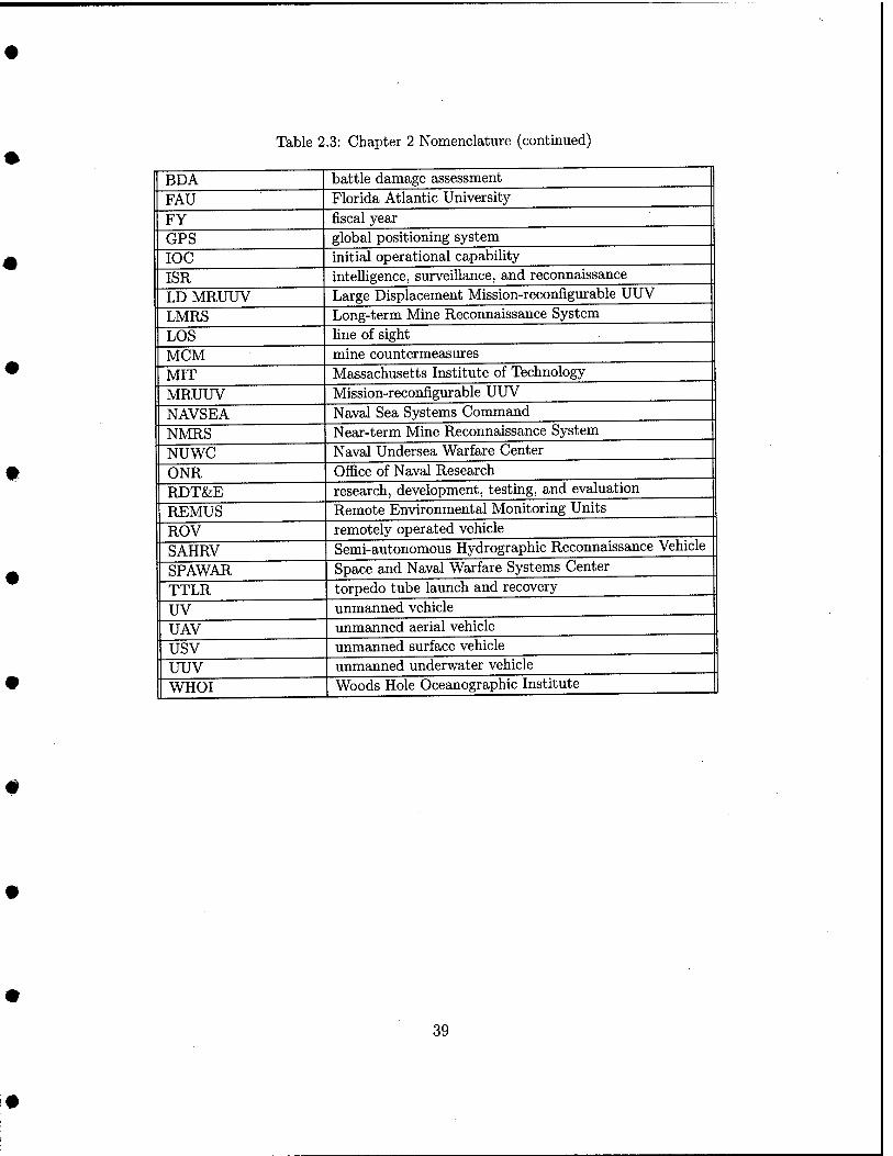
Table 2.3: Chapter 2 Nomenclature (continued)
BDA battle damage assessment FAU Florida Atlantic University FY fiscal year GPS global positioning system IOC initial operational capability ISR intelligence, surveillance, and reconnaissance LD MRUUV Large Displacement Mission-reconfigurable UUV
LMRS Long-term Mine Reconnaissance System
LOS line of sight MCM mine countermeasures MIT Massachusetts Institute of Technology MRUUV Mission-reconfigurable UUV
NAVSEA Naval Sea Systems Command NMRS Near-term Mine Reconnaissance System
NUWC Naval Undersea Warfare Center
ONR Office of Naval Research RDT&E research, development, testing, and evaluation
REMUS Remote Environmental Monitoring Units
ROV remotely operated vehicle
SAHRV Semi-autonomous Hydrographic Reconnaissance Vehicle
SPAWAR Space and Naval Warfare Systems Center
TTLR torpedo tube launch and recovery
UV unmanned vehicle UAV unmanned aerial vehicle
USV unmanned surface vehicle
UUV unmanned underwater vehicle
WHOI Woods Hole Oceanographic Institute
39

This page intentionally blank
40

Chapter 3
Analysis of Alternative Designs
3.1 Design Goals and Requirements The AUV recharge system design problem was defined by the following set of requirements and goals:
1. System must be mechanically and electrically compatible with all present and near-term future U.S. Navy AUVs.
2. System must be capable of autonomous docking, battery recharging, and undocking.
3. System must be operable over the same depth range as the AUVs it services.
4. System must be robust and reliable enough for extended, unattended deployment in the ocean.
5. System should minimize required back-fit modifications to AUVs.
6. Docking mechanism should use the fewest moving parts possible.
7. AU docking and undocking power requirements should be supplied by the dock, not the AUV.
8. Latching operation should be passive.
9. Undocking operation should require positive action by the dock.
10. Entire system must be deployable on the tanker AUV (described in section 2.1.3).
11. In the default failure condition (i.e., loss of power by the dock or AUV), the AUV stays securely fixed to the dock.
The design problem was broken into two segments: the mechanical capture and alignment mechanism, and the electrical power coupling mechanism. The two areas are dependent on each other, since the electrical couphng will dictate a certain mechanical alignment or position.
Two categories of electrical power coupling mechanisms were considered: wet-mateable conduc- tive pin connectors, and inductive couplings. Both mechanisms have advantages and disadvantages, and both have been used in previous docking system designs. The pros and cons of each are sum- marized in Table 3.1.
41
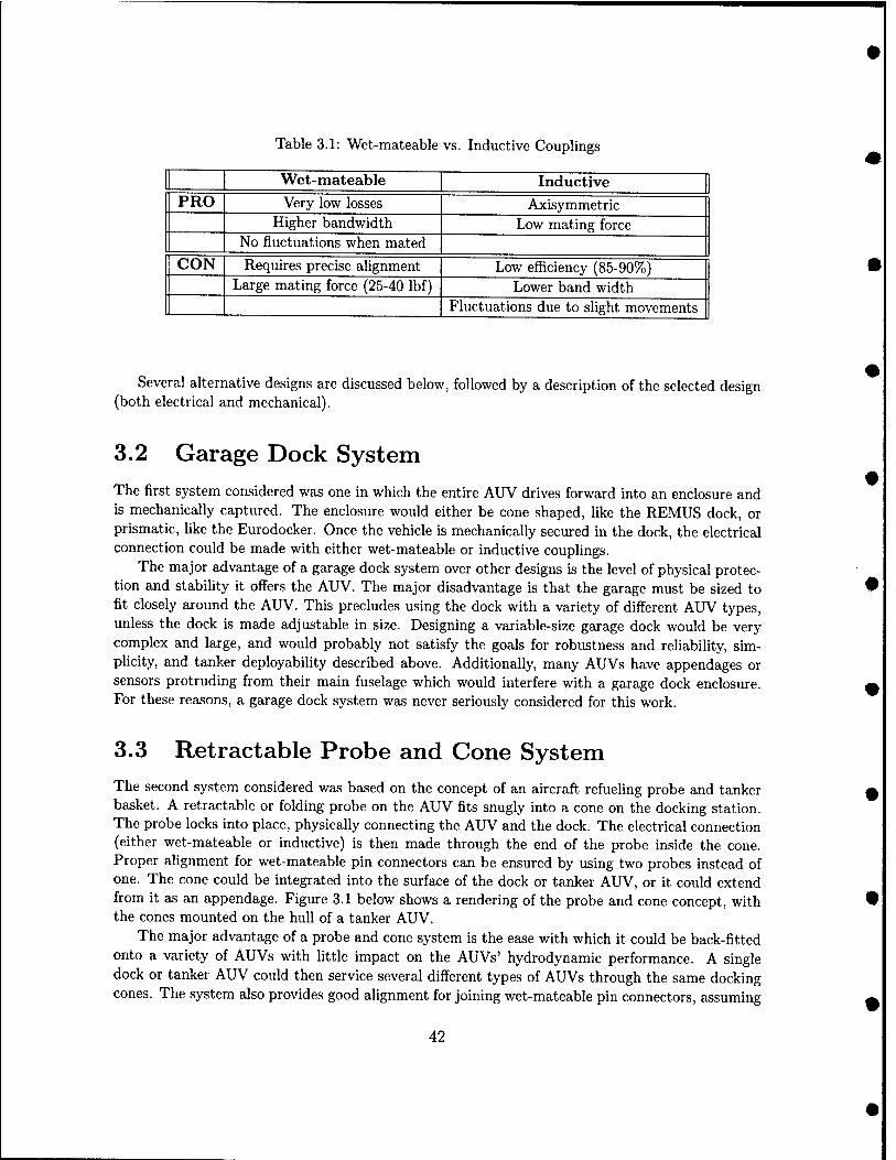
Table 3.1: Wet-mateable vs. Inductive Couplings
PRO
CON
Wet-mateable Very low losses
Higher bandwidth No fluctuations when mated
Requires precise alignment Large mating force (25-40 Ibf)
Inductive
Axisymmetric Low mating force
Low efficiency (85-90%) Lower band width
Fluctuations due to slight movements
Several alternative designs are discussed below, followed by a description of the selected design (both electrical and mechanical).
3.2 Garage Dock System
The first system considered was one in which the entire AUV drives forward into an enclosure and is mechanically captured. The enclosure would either be cone shaped, like the REMUS dock, or prismatic, like the Eurodocker. Once the vehicle is mechanically secured in the dock, the electrical connection could be made with either wet-mateable or inductive couplings.
The major advantage of a garage dock system over other designs is the level of physical protec- tion and stability it offers the AUV. The major disadvantage is that the garage must be sized to fit closely around the AUV. This precludes using the dock with a variety of different AUV types, unless the dock is made adjustable in size. Designing a variable-size garage dock would be very complex and large, and would probably not satisfy the goals for robustness and reliability, sim- plicity, and tanker deployability described above. Additionally, many AUVs have appendages or sensors protruding from their main fuselage which would interfere with a garage dock enclosure. For these reasons, a garage dock system was never seriously considered for this work.
3.3 Retractable Probe and Cone System The second system considered was based on the concept of an aircraft refueling probe and tanker basket. A retractable or folding probe on the AUV fits snugly into a cone on the docking station. The probe locks into place, physically connecting the AUV and the dock. The electrical connection (either wet-mateable or inductive) is then made through the end of the probe inside the cone. Proper alignment for wet-mateable pin connectors can be ensured by using two probes instead of one. The cone could be integrated into the surface of the dock or tanker AUV, or it could extend from it as an appendage. Figure 3.1 below shows a rendering of the probe and cone concept, with the cones mounted on the hull of a tanker AUV.
The major advantage of a probe and cone system is the ease with which it could be back-fitted onto a variety of AUVs with little impact on the AUVs' hydrodynamic performance. A single dock or tanker AUV could then service several different types of AUVs through the same docking cones. The system also provides good alignment for joining wet-mateable pin connectors, assuming
42
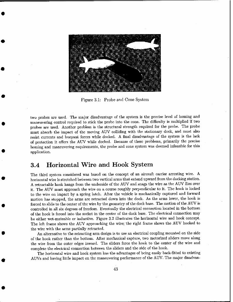
Figure 3.1: Probe and Cone System
two probes are used. The major disadvantage of tlie system is the precise level of homing and maneuvering control required to stick the probe into the cone. The difficulty is multipUed if two probes are used. Another problem is the structural strength required for the probe. The probe must absorb the impact of the moving AUV coUiding with the stationary dock, and must also resist currents and buoyant forces while docked. A final disadvantage of the system is the lack of protection it offers the AUV while docked. Because of these problems, primarily the precise homing and maneuvering requirements, the probe and cone system was deemed infeasible for this application.
3.4 Horizontal Wire and Hook System The third system considered was based on the concept of an aircraft carrier arresting wire. A horizontal wire is stretched between two vertical arms that extend upward from the docking station. A retractable hook hangs from the underside of the AUV and snags the wire as the AUV flies over it. The AUV mast approach the wire on a course roughly perpendicular to it. The hook is locked to the wire on impact by a spring latch. After the vehicle is mechanically captured and forward motion has stopped, the arms are retracted down into the dock. As the arms lower, the hook is forced to slide to the center of the wire by the geometry of the dock base. The motion of the AUV is controlled in all six degrees of freedom. Eventually the electrical connection located in the bottom of the hook is forced into the socket in the center of the dock base. The electrical connection may be either wet-mateable or inductive. Figure 3.2 illustrates the horizontal wire and hook concept. The left frame shows the AUV approaching the wire; the right frame shows the AUV hooked to the wire with the arms partially retracted.
An alternative to the retracting arm design is to use an electrical couphng mounted on the side of the hook rather than the bottom. After mechanical capture, two motorized shders move along the wire from the outer edges inward. The sliders force the hook to the center of the wire and complete the electrical connection between the sliders and the side of the hook.
The horizontal wire and hook system has the advantages of being easily back-fitted to existing AUVs and having little impact on the maneuvering performance of the AUV. The major disadvan-
43
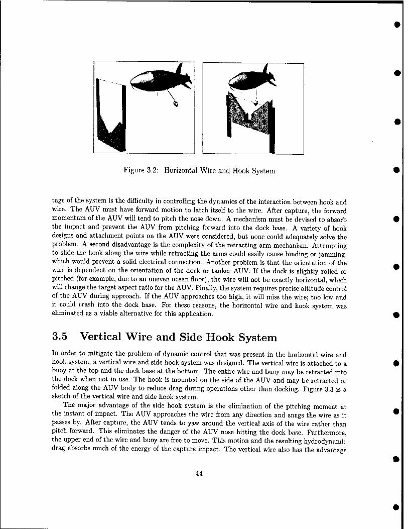
Figure 3.2: Horizontal Wire and Hook System
tage of the system is the difficulty in controlling the dynamics of the interaction between hook and wire. The AUV must have forward motion to latch itself to the wire. After capture, the forward momentum of the AUV will tend to pitch the nose down. A mechanism must be devised to absorb the impact and prevent the AUV from pitching forward into the dock base. A variety of hook designs and attachment points on the AUV were considered, but none could adequately solve the problem. A second disadvantage is the complexity of the retracting arm mechanism. Attempting to slide the hook along the wire while retracting the arms could easily cause binding or jamming, which would prevent a solid electrical connection. Another problem is that the orientation of the wire is dependent on the orientation of the dock or tanker AUV. If the dock is slightly rolled or pitched (for example, due to an uneven ocean floor), the wire will not be exactly horizontal, which will change the target aspect ratio for the AUV. Finally, the system requires precise altitude control of the AUV during approach. If the AUV approaches too high, it will miss the wire; too low and it could crash into the dock base. For these reasons, the horizontal wire and hook system was eliminated as a viable alternative for this application.
3.5 Vertical Wire and Side Hook System In order to mitigate the problem of dynamic control that was present in the horizontal wire and hook system, a vertical wire and side hook system was designed. The vertical wire is attached to a buoy at the top and the dock base at the bottom. The entire wire and buoy may be retracted into the dock when not in use. The hook is mounted on the side of the AUV and may be retracted or folded along the AUV body to reduce drag during operations other than docking. Figure 3.3 is a sketch of the vertical wire and side hook system.
The major advantage of the side hook system is the elimination of the pitching moment at the instant of impact. The AUV approaches the wire from any direction and snags the wire as it passes by After capture, the AUV tends to yaw around the vertical axis of the wire rather than pitch forward. This eliminates the danger of the AUV nose hitting the dock base. Furthermore, the upper end of the wire and buoy are free to move. This motion and the resulting hydrodynamic drag absorbs much of the energy of the capture impact. The vertical wire also has the advantage
44
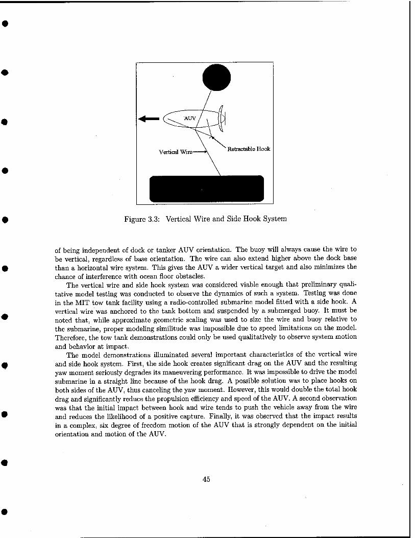
Retractable Hook
Figure 3.3: Vertical Wire and Side Hook System
of being independent of dock or tanker AUV orientation. The buoy will always cause the wire to be vertical, regardless of base orientation. The wire can also extend higher above the dock base than a horizontal wire system. This gives the AUV a wider vertical target and also minimizes the chance of interference with ocean floor obstacles.
The vertical wire and side hook system was considered viable enough that preliminary quali- tative model testing was conducted to observe the dynamics of such a system. Testing was done in the MIT tow tank facihty using a radio-controlled submarine model fitted with a side hook. A vertical wire was anchored to the tank bottom and suspended by a submerged buoy. It must be noted that, while approximate geometric scaling was used to size the wire and buoy relative to the submarine, proper modehng similitude was impossible due to speed Umitations on the model. Therefore, the tow tank demonstrations could only be used qualitatively to observe system motion and behavior at impact.
The model demonstrations illuminated several important characteristics of the vertical wire and side hook system. First, the side hook creates significant drag on the AUV and the resulting yaw moment seriously degrades its maneuvering performance. It was impossible to drive the model submarine in a straight line because of the hook drag. A possible solution was to place hooks on both sides of the AUV, thus canceling the yaw moment. However, this would double the total hook drag and significantly reduce the propulsion efficiency and speed of the AUV. A second observation was that the initial impact between hook and wire tends to push the vehicle away from the wire and reduces the likehhood of a positive capture. Finally, it was observed that the impact results in a complex, six degree of freedom motion of the AUV that is strongly dependent on the initial orientation and motion of the AUV.
45
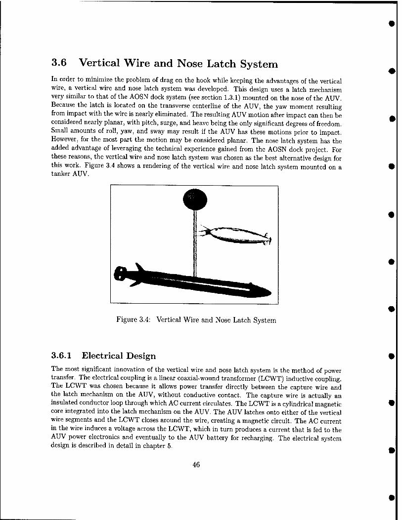
3.6 Vertical Wire and Nose Latch System
In order to minimize the problem of drag on the hook while keeping the advantages of the vertical wire, a vertical wire and nose latch system was developed. This design uses a latch mechanism very similar to that of the AOSN dock system (see section 1.3.1) mounted on the nose of the AUV. Because the latch is located on the transverse centerline of the AUV, the yaw moment resulting from impact with the wire is nearly eliminated. The resulting AUV motion after impact can then be considered nearly planar, with pitch, surge, and heave being the only significant degrees of freedom. Small amounts of roll, yaw, and sway may result if the AUV has these motions prior to impact. However, for the most part the motion may be considered planar. The nose latch system has the added advantage of leveraging the technical experience gained from the AOSN dock project. For these reasons, the vertical wire and nose latch system was chosen as the best alternative design for this work. Figure 3.4 shows a rendering of the vertical wire and nose latch system mounted on a tanker AUV.
Figure 3.4: Vertical Wire and Nose Latch System
3.6.1 Electrical Design
The most significant innovation of the vertical wire and nose latch system is the method of power transfer. The electrical coupling is a hnear coaxial-wound transformer (LCWT) inductive coupling. The LCWT was chosen because it allows power transfer directly between the capture wire and the latch mechanism on the AUV, without conductive contact. The capture wire is actually an insulated conductor loop through which AC current circulates. The LCWT is a cylindrical magnetic core integrated into the latch mechanism on the AUV. The AUV latches onto either of the vertical wire segments and the LCWT closes around the wire, creating a magnetic circuit. The AC current in the wire induces a voltage across the LCWT, which in turn produces a current that is fed to the AUV power electronics and eventually to the AUV battery for recharging. The electrical system design is described in detail in chapter 5.
46
3.6.2 Mechanical Design The wire mechanism is the same as described above in section 3.5, except that the single capture wire is now replaced with a loop. The upper end of the loop is attached to a float and is extended upward from the docking station or tanker AUV. The two lower ends of the wire loop extend into the dock base and are connected to the AC power supply. The wire remains vertical due to the buoyancy of the float, regardless of base orientation. The AUV may hit the wire anywhere along its vertical length. The stiffness and damping of the system are controlled by the wire length and buoy size and shape. Chapter 4 describes the after-impact motion of the AUV in detail.
The latch mechanism consists of two sets of V-shaped arms with spring-loaded capture bars mounted on the nose of the AUV. The latch mechanism could eventually be designed to retract or fold along the AUV sides when not in use. The AUV drives directly into the vertical wire and its forward motion pushes the capture bars aside, positively latching the AUV to the wire. Undocking is accomphshed by opening the capture bars with a rotary actuator, then backing the AUV away firom the wire. The mechanical design of the latch mechanism is described in detail in chapter 7.
47

This page intentionally blank
48
Chapter 4
Mechanical Dynamic ModeUng and Simulation
In order to quickly and easily analyze the dynamic behavior of the proposed docking system over a range of operating conditions, a computer simulation was created. The main goal of the simulation was to ensure that the system does not exceed allowable deflections or cable tensions under any foreseeable operating conditions. A secondary goal of the simulation was to compute a gross estimate of the forces and moments acting at the AUV-cable interface. This simulation was done using Matlab computational software. All Matlab codes are shown in Appendix A. The finished product allowed the user to vary all key parameters of the system, including cable length and diameter, buoy diameter and mass, AUV velocity, and drag coefficients. The simulation model was a valuable design tool in selecting the physical characteristics of the docking system.
A complete fist of all nomenclature used in this chapter is found in section 4.6.
4.1 System Geometry and Assumptions The comphcated three-dimensional kinematics of the real system were reduced to a simplified planar model for purposes of the computer simulation. The reduction results in much simpler and more straightforward equations of motion, while retaining all significant information pertinent to the system design. The planar model has four dynamic degrees of freedom (DOFs): ^i, h, h, and 62- All other system positions, velocities, and accelerations can be expressed in terms of these DOFs and their derivatives. Figure 4.1 below illustrates the simplified system geometry.
A number of assumptions were required to reduce the problem from three dimensions to two and to limit the number of DOFs to four. First, it was assumed that the two cable sections, Li and L2, remain straight links throughout the transient, with no cable curvature. This is a vaUd assumption given the relatively short length of cable. Each link is treated as a Unear spring-viscous damper system, with 5i and 82 being the extension lengths of each link. The spring constants, k, were calculated using the equation:
EA ^ = -L
where E=Young's modulus of the cable, A=cable cross-sectional area, and L=unstretched segment length. The viscous damping constants, c, were calculated as a fraction of critical damping using
49
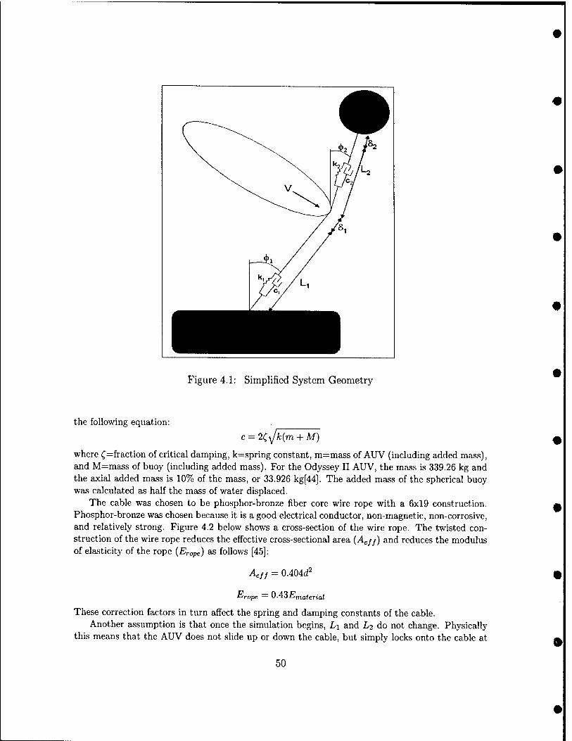
Figure 4.1: Simplified System Geometry
the following equation:
c = 2C,sJk{m + M)
where C=fraction of critical damping, k=spring constant, m=mass of AUV (including added mass), and M=mass of buoy (including added mass). For the Odyssey II AUV, the mass is 339.26 kg and the axial added mass is 10% of the mass, or 33.926 kg[44]. The added mass of the spherical buoy was calculated as half the mass of water displaced.
The cable was chosen to be phosphor-bronze fiber core wire rope with a 6x19 construction. Phosphor-bronze was chosen because it is a good electrical conductor, non-magnetic, non-corrosive, and relatively strong. Figure 4.2 below shows a cross-section of the wire rope. The twisted con- struction of the wire rope reduces the effective cross-sectional area [Aeff) and reduces the modulus of elasticity of the rope [Erape) as follows [45]:
Aefi - 0.404^2
These correction factors in turn affect the spring and damping constants of the cable. Another assumption is that once the simulation begins, L\ and L2 do not change. Physically
this means that the AUV does not slide up or down the cable, but simply locks onto the cable at
50
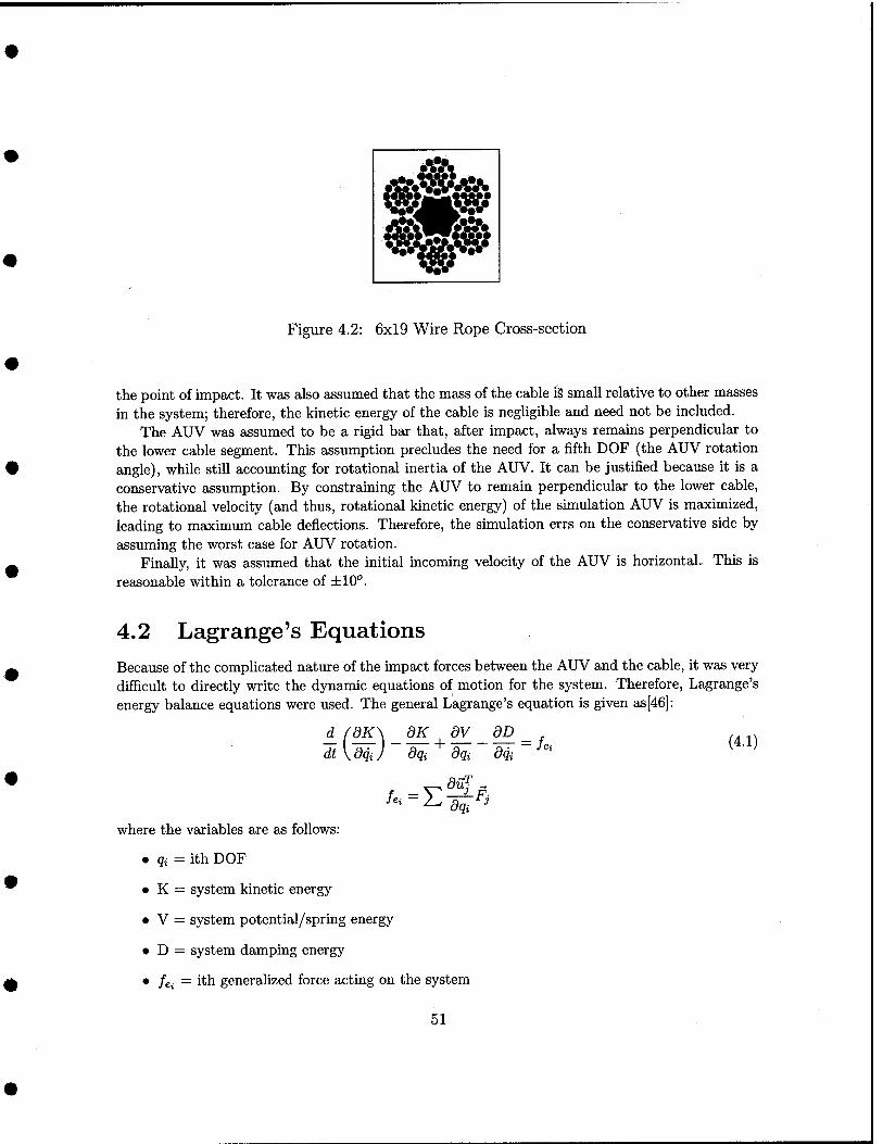
Figure 4.2: 6x19 Wire Rope Cross-section
the point of impact. It was also assumed that the mass of the cable i§ small relative to other masses in the system; therefore, the kinetic energy of the cable is negligible and need not be included.
The AUV was assumed to be a rigid bar that, after impact, always remains perpendicular to the lower cable segment. This assumption precludes the need for a fifth DOF (the AUV rotation angle), while still accounting for rotational inertia of the AUV. It can be justified because it is a conservative assumption. By constraining the AUV to remain perpendicular to the lower cable, the rotational velocity (and thus, rotational kinetic energy) of the simulation AUV is maximized, leading to maximum cable deflections. Therefore, the simulation errs on the conservative side by assuming the worst case for AUV rotation.
Finally, it was assumed that the initial incoming velocity of the AUV is horizontal. This is reasonable within a tolerance of ±10°.
4.2 Lagrange's Equations Because of the comphcated nature of the impact forces between the AUV and the cable, it was very difficult to directly write the dynamic equations of motion for the system. Therefore, Lagrange's energy balance equations were used. The general Lagrange's equation is given as[46]:
dt dK\ dK dV_ dD^ dcji) dqi dqi dqi
(4.1)
dqi
where the variables are as follows:
• qi = ith DOF
• K = system kinetic energy
• V = system potential/spring energy
• D — system damping energy
• /ei = ith generalized force acting on the system
51
• Uj = jth displacement coordinate
• Fj = jth external force acting on the system
• T superscript indicates matrix transpose
The general equation is applied to each of n DOFs to yield a total of n 2"*^ order ordinary differential equations (ODEs). In the case of this simulation, the ODEs were solved numerically using variable order numerical differentiation formulae. This technique is conveniently available in the Matlab odesolver functions.
4.2.1 Kinetic Energy As discussed earlier, the kinetic energy of the cable was neglected due to its small mass. Therefore, the only elements of the system possessing kinetic energy are the AUV and the buoy, both in translation and rotation. The general expression for kinetic energy is
K = -mv^ + -iJ^
The velocities of the AUV and buoy must be expressed in terms of the dynamic DOFs: (f>i, (t>2, S\, and 62-
The velocity of the AUV is straightforward, and may be written as:
VAUV ~ [Li + 6i)4>iet + Sie'n
where it and e'„ are the unit vectors perpendicular and parallel to L\, respectively. The velocity of the buoy becomes a complicated function of 0i, <^2, <5i, and 62. The buoy has
a velocity component perpendicular to Lj and a component parallel to Li. The perpendicular component can be written as:
Vperp = (Ll + Si)<j)i + (L2 + (52)02 C0s((/>1 - ^2) - ^2 sin(0i - (^2)
The parallel component can be written as:
Vpar = {L2 + 52)(?i2 Sin(0i - (j)2) + 6\ + 62 COs{<j)i - ^2)
The total buoy velocity may then be written as:
vCoy = \{L\ + <5l)<^l + (L2 + 52)<j>2 cos(0i - 4>2) - 62 sm{(f>i - ^2)] et
+ [{L2 + 62)4)2 sin(0i - <f)2) + ^'1 + 82 cos((/)i - (f)2)] e'n
Figure 4.3 shows the system velocity components. If m = the mass of the AUV (including axial added mass), M = the mass of the buoy (including
added mass), IAUV = the mass moment of inertia of the AUV about its nose, and Ibuoy = the mass moment of inertia of the buoy, then the total kinetic energy of the system can be written as:
-m IvAuvl"^ + -^M \vbuov? + ^IAUVC^I"^ + -^T K =-m \VAUV\'^ + -xM l^buoyl^ + -^lAUV<i>\ + ■xlbuay(^2 (4.2)
The mass moment of inertia of the Odyssey II AUV about its nose is 398.29kg - m^[44]. The mass moment of inertia of the spherical buoy was calculated as:
/.. = ?M(^)'
52
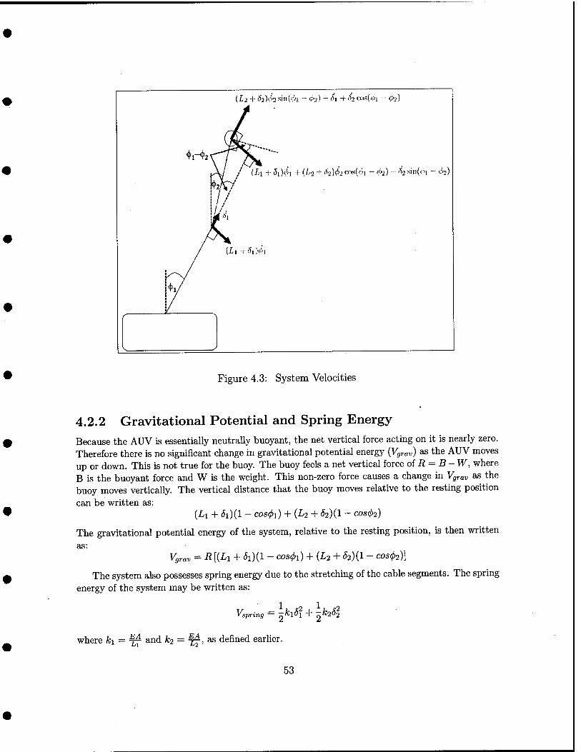
{L'2 + 52)<1>2si!l((»l - (?:>) +(^1+52 COS(01 - <f>2)
/ (ij +5i)4>] +{L2 + S2)'h<-M<i'\ -4>2]-S2^riiJn -Si)
Figure 4.3: System Velocities
4.2.2 Gravitational Potential and Spring Energy Because the AUV is essentially neutrally buoyant, the net vertical force acting on it is nearly zero. Therefore there is no significant change in gravitational potential energy (Vgrav) as the AUV moves up or down. This is not true for the buoy. The buoy feels a net vertical force oiR = B-W, where B is the buoyant force and W is the weight. This non-zero force causes a change in Vgrav as the buoy moves vertically. The vertical distance that the buoy moves relative to the resting position can be written as:
(Li + (5l)(l - COS^l) + (L2 + <52)(1 - COS02)
The gravitational potential energy of the system, relative to the resting position, is then written as:
Vgrav = R [{Ll + Sl){l - COS(t>i) + (L2 + ^2)(1 - C0S(f)2)]
The system also possesses spring energy due to the stretching of the cable segments. The spring energy of the system may be written as:
v; spring — o"-!"! + 9^ ^
where ki = ^ and A;2 = 7;^, as defined earlier.
53
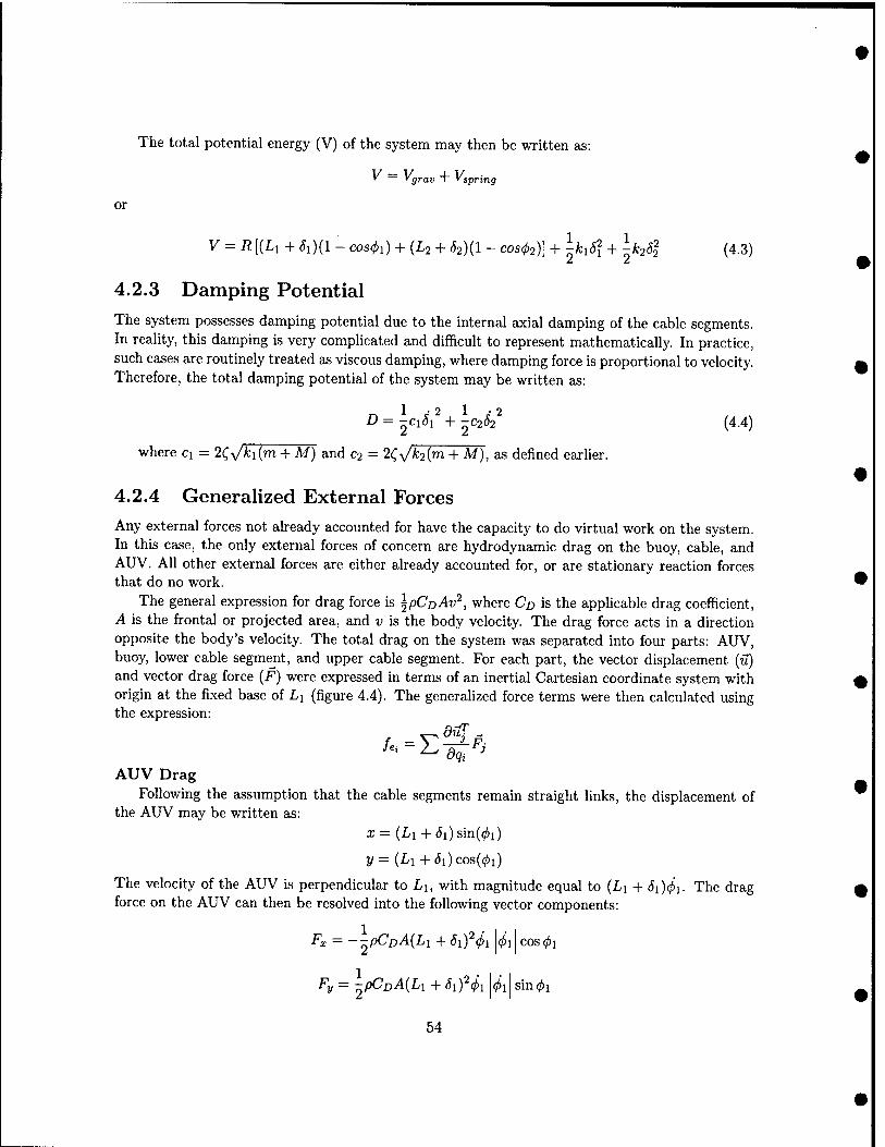
or
The total potential energy (V) of the system may then be written as:
•■^ ~ 'grav + '^spring
V = i?[(Li + 6i){l - COS(t>i) + (L2 + 52){l - CO502)] + \h5\ + \k2&l (4.3)
4.2.3 Damping Potential
The system possesses damping potential due to the internal axial damping of the cable segments. In reality, this damping is very complicated and difficult to represent mathematically. In practice, such cases are routinely treated as viscous damping, where damping force is proportional to velocity. Therefore, the total damping potential of the system may be written as:
1 2 1 -2 ^=2^i<5i +2^2(52 (4.4)
where cx = 2CV'fci(m + M) and C2 = 2C\/A;2(m +M), as defined earlier.
4.2.4 Generalized External Forces
Any external forces not already accounted for have the capacity to do virtual work on the system. In this case, the only external forces of concern are hydrodynamic drag on the buoy, cable, and AUV. All other external forces are either already accounted for, or are stationary reaction forces that do no work.
The general expression for drag force is ^pCoAv'^, where Co is the applicable drag coefficient, A is the frontal or projected area, and v is the body velocity. The drag force acts in a direction opposite the body's velocity. The total drag on the system was separated into four parts: AUV, buoy, lower cable segment, and upper cable segment. For each part, the vector displacement (u) and vector drag force (F) were expressed in terms of an inertial Cartesian coordinate system with origin at the fixed base of Li (figure 4.4). The generahzed force terms were then calculated using the expression:
diff ^
AUV Drag Following the assumption that the cable segments remain straight links, the displacement of
the AUV may be written as: X- (Li + 6i)sm{<j)i)
y = {Lx + (5i)cos(0i)
The velocity of the AUV is perpendicular to Li, with magnitude equal to {Lx + &x)4>\- The drag force on the AUV can then be resolved into the following vector components:
Fx = --pCDA{Lx-\-8xf^x |0i|cos0i
^v = -x(^DA{Lx + 5xf(i>x |«!f>i|sin^i
54
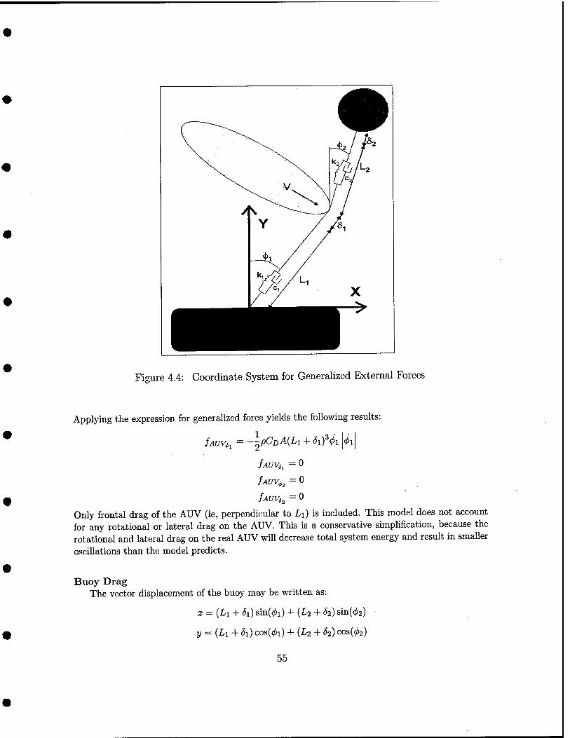
Figure 4.4: Coordinate System for Generalized External Forces
Applying the expression for generalized force yields the following results:
fAUVs^ = 0
fAUV^2 ^ ^
fAUVi ■52 0
Only frontal drag of the AUV (ie, perpendicular to Li) is included. This model does not account for any rotational or lateral drag on the AUV. This is a conservative simplification, because the rotational and lateral drag on the real AUV will decrease total system energy and result in smaller oscillations than the model predicts.
Buoy Drag The vector displacement of the buoy may be written as:
x = {Li + 6i) sm{(j)i) + (L2 + 52) sin((;i2)
j/ = (Li + 5i) cos{(i)i) + (L2 + ^2) cos(^2)
55
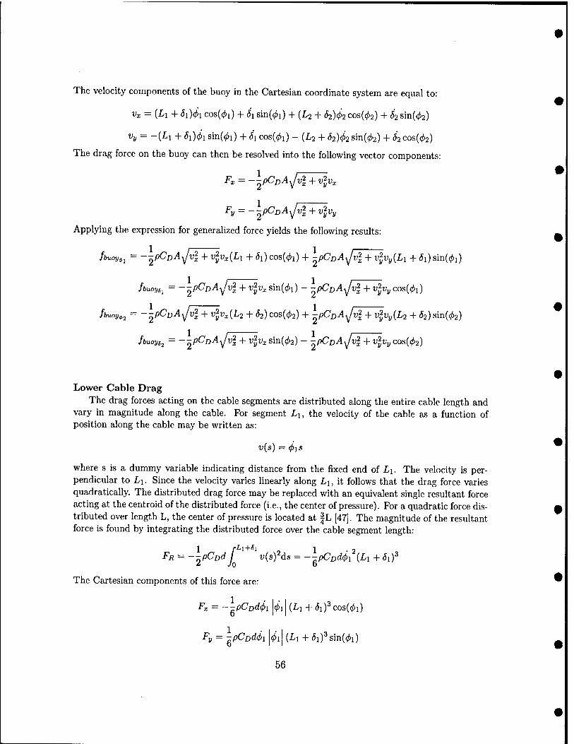
The velocity components of the buoy in the Cartesian coordinate system are equal to:
Vx = (Li + Si)4>icos{4>i) + Sism{(l)i) + {L2 + 62)4>2Cos{<j)2) + 62sm{(l)2)
'Vy = -(^1 + h)<i>i sin((/.i) + 5x cos(0i) - (L2 + 82)^ ^M<t>2) + ^2 cos((?!>2)
The drag force on the buoy can then be resolved into the following vector components:
Fx = --pCoA^vl + vlv^
Fy = --pCoA^vl + vlvy
Applying the expression for generalized force yields the following results:
fbuoy^^ = -I^PCDA^V1^VIVX{LI + 8i)cos{4>i) + -pCDA^vl + v^VyiLi + Si)sm{(j)i)
huoye, = --pCoA^vl + vlv^ sin(0i) - -pCoAyJvl + vlvy cos(0i)
fbuoy^^ = -■J^PCDASJVI + VIV^{L2 + ^2) C0s((?!.2) + -pCDAsp[+^^Vy{L2 + 82) sin(02)
fbuoys^ = --pCoA^Jvl + v^t;^ sin(02) - -pCoA^vl + v^Vy cos(02)
Lower Cable Drag The drag forces acting on the cable segments are distributed along the entire cable length and
vary in magnitude along the cable. For segment Li, the velocity of the cable as a function of position along the cable may be written as:
v{s) = 4>is
where s is a dummy variable indicating distance from the fixed end of Li. The velocity is per- pendicular to Li. Since the velocity varies hnearly along Li, it follows that the drag force varies quadratically. The distributed drag force may be replaced with an equivalent single resultant force acting at the centroid of the distributed force (i.e., the center of pressure). For a quadratic force dis- tributed over length L, the center of pressure is located at |L [47]. The magnitude of the resultant force is found by integrating the distributed force over the cable segment length:
FR = --pCodj v{sfds = --pCDd(t>i (Li + 6,)^
The Cartesian components of this force are:
Fx = —^pCDd4>i U'l (Li + (5if cos(0i) 6'
1 6'
Fy = -pCpdcpi Ui| (Li + (5i)^sin(0i)
56
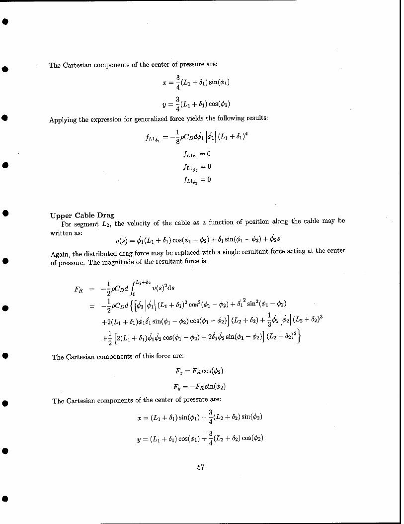
The Cartesian components of the center of pressure are:
3 a; = -(Li + di)sin(</)i)
3 j/ = -(Li + 5i)cos(0i)
Applying the expression for generaUzed force yields the following results:
fLi,,=-\pCDd4>i\h\{Li + Sr)'
Upper Cable Drag For segment L2, the velocity of the cable as a function of position along the cable may be
written as: . . v{s) = 4>i{Li + 5i) cos(0i - 02) + (5i sin((^i - (1)2) + 4>2S
Again, the distributed drag force may be replaced with a single resultant force acting at the center of pressure. The magnitude of the resultant force is:
FR = -TipCnd / v{syds 2 Jo
= -ipCjodlU Ui I (Li + (5i)^cos2 ((^1-02) +5i^sin2((/>!-(/)2)
^ 1 • I • I +2(Li + Si)4>i5i sm{(l)i - <j)2) cos((^i - h)] {L2 + h) + ^4>2 \4>2\ {L2 + ^2)^
+- [2(Li + 5i)<i)i^2 cos(0i - 02) + 2<5"i02 sin(0i - ^2)] (^2 + hf\
The Cartesian components of this force are:
F,-FRCOS(02)
Fj; = -Fiisin(02)
The Cartesian components of the center of pressure are:
3 x = {Li + 5i) sin((?!>i) + -(L2 + 62) sin(02)
3 y = (Li + 5l) COs(0l) + -(L2 + ^2) COs[<t)2)
57
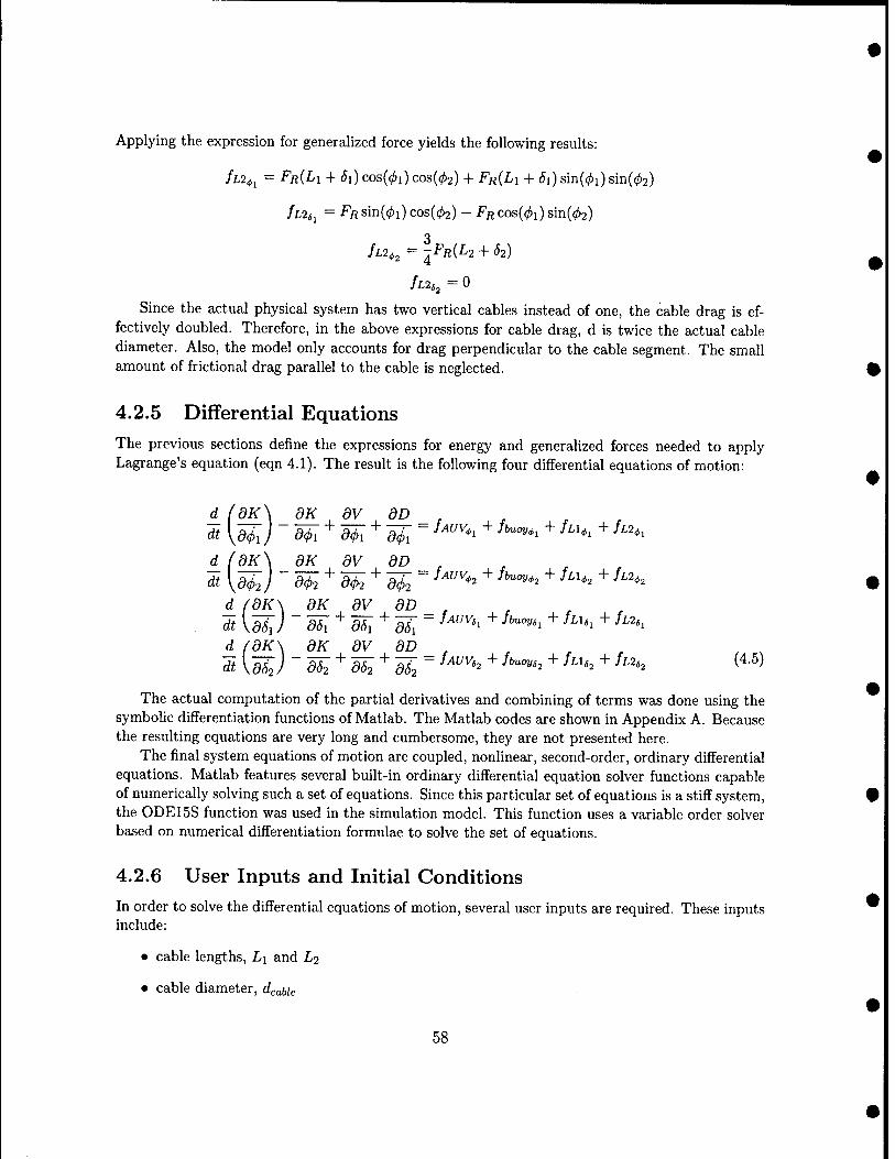
Applying the expression for generalized force yields the following results:
SL2^^ = FR{LI + 8{)co?.{<j)i)cos{(t>2) + Fa{Li + 5i) sin(^i) sin(02)
/wsj = Ffisin(0i)cos(</)2) - FRC0s((/)i)sin((?l)2)
/L2^3 = -^FR{L2 + 52)
/L2,, = 0
Since the actual physical system has two vertical cables instead of one, the cable drag is ef- fectively doubled. Therefore, in the above expressions for cable drag, d is twice the actual cable diameter. Also, the model only accounts for drag perpendicular to the cable segment. The small amount of frictional drag parallel to the cable is neglected.
4.2.5 Differential Equations
The previous sections define the expressions for energy and generalized forces needed to apply Lagrange's equation (eqn 4.1). The result is the following four differential equations of motion:
't'l
d (dK\ OK dV dD _
dt [d^J ~Wi'^Wi^dh~ '' "^ ""*' ^ *' "^ d (dK\ dK dV dD _
dt \d<i>2 J'dh'^dh'^dh' "' ^ "''" "^ -^^'^^ ^ ^^'*^ d (dK\ dK dV dD ^
dt \mj "Ml^ml^'MT '' ^^'"""'^ ^-^^''^ ^^"'' d (dK\ dK dV dD . ^ r r
'dt Va^j ~ aj^ + a^ + 5^ ^ -^^^^^^ + ^'"'^^^ + -^^^^^ + ^"^^ (^-^^
The actual computation of the partial derivatives and combining of terms was done using the symbolic differentiation functions of Matlab. The Matlab codes are shown in Appendix A. Because the resulting equations are very long and cumbersome, they are not presented here.
The final system equations of motion are coupled, nonhnear, second-order, ordinary differential equations. Matlab features several built-in ordinary differential equation solver functions capable of numerically solving such a set of equations. Since this particular set of equations is a stiff system, the 0DE15S function was used in the simulation model. This function uses a variable order solver based on numerical differentiation formulae to solve the set of equations.
4.2.6 User Inputs and Initial Conditions
In order to solve the differential equations of motion, several user inputs are required. These inputs include:
• cable lengths, Li and L2
• cable diameter, dcaUe
58
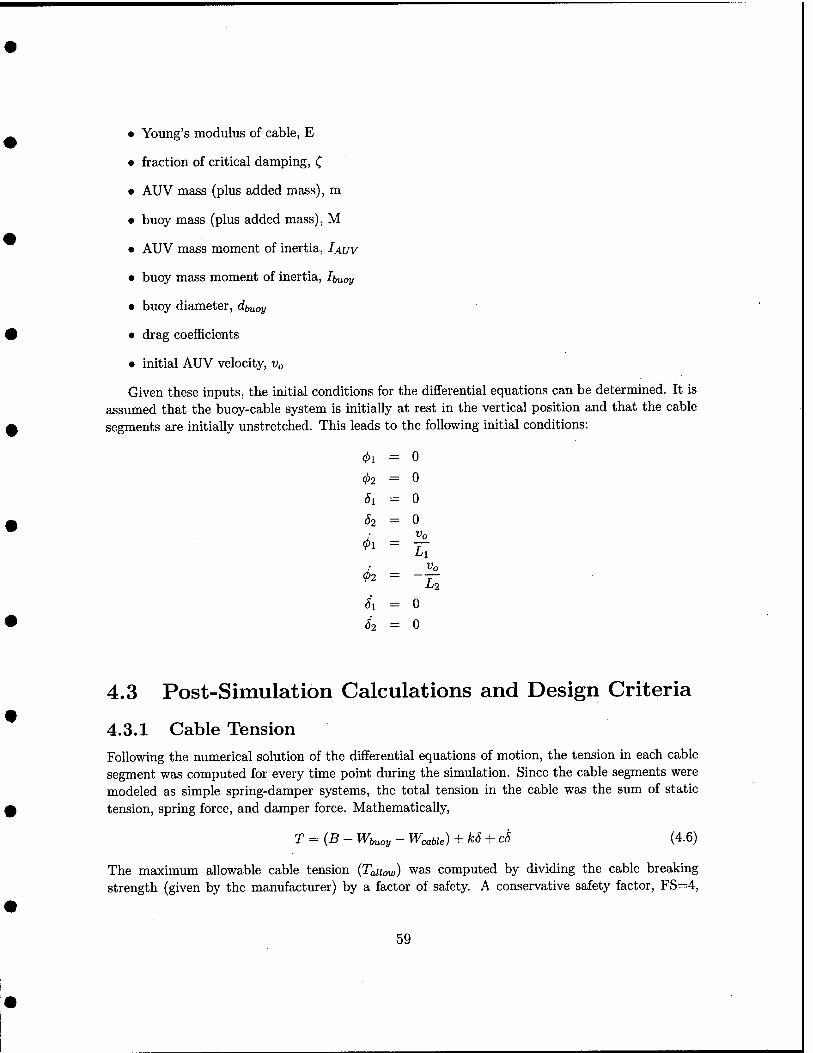
• Young's modulus of cable, E
• fraction of critical damping, C
• AUV mass (plus added mass), m
• buoy mass (plus added mass), M
• AUV mass moment of inertia, IAUV
• buoy mass moment of inertia, Ibuoy
• buoy diameter, dtmay
• drag coefficients
• initial AUV velocity, Vo
Given these inputs, the initial conditions for the differential equations can be determined. It is assumed that the buoy-cable system is initially at rest in the vertical position and that the cable segments are initially unstretched. This leads to the following initial conditions:
<^i = 0
02-0
61 = 0
62 ^ 0
^^ = I^ A. ^° ^' = -T, Si = 0
62 = 0
4.3 Post-Simulation Calculations and Design Criteria
4.3.1 Cable Tension Following the numerical solution of the differential equations of motion, the tension in each cable segment was computed for every time point during the simulation. Since the cable segments were modeled as simple spring-damper systems, the total tension in the cable was the sum of static tension, spring force, and damper force. Mathematically,
T={B- Wbuoy - WcaUe) + k5 + c5 (4.6)
The maximum allowable cable tension {Taiiaw) was computed by dividing the cable breaking strength (given by the manufacturer) by a factor of safety. A conservative safety factor, FS=4,
59
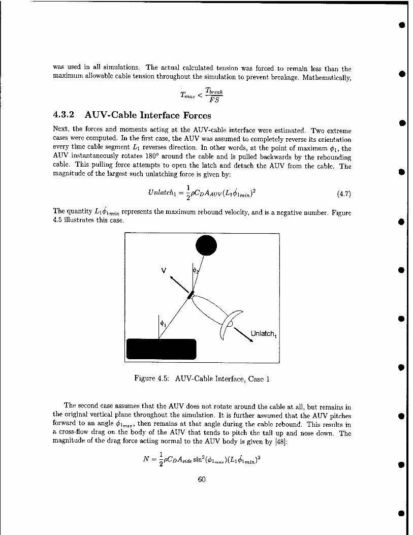
was used in all simulations. The actual calculated tension was forced to remain less than the maximum allowable cable tension throughout the simulation to prevent breakage. Mathematically,
J-max *^ ^ break
FS
4.3.2 AUV-Cable Interface Forces
Next, the forces and moments acting at the AUV-cable interface were estimated. Two extreme cases were computed. In the first case, the AUV was assumed to completely reverse its orientation every time cable segment Li reverses direction. In other words, at the point of maximum 4>i, the AUV instantaneously rotates 180° around the cable and is pulled backwards by the rebounding cable. This pulling force attempts to open the latch and detach the AUV from the cable. The magnitude of the largest such unlatching force is given by:
Unlatchi = -pCDAAuv{Li(j)i^in) (4.7)
The quantity Li(/>i^;„ represents the maximum rebound velocity, and is a negative number. Figure 4.5 illustrates this case.
Unlatch-
Figure 4.5: AUV-Cable Interface, Case 1
The second case assumes that the AUV does not rotate around the cable at all, but remains in the original vertical plane throughout the simulation. It is further assumed that the AUV pitches forward to an angle ^i„„^, then remains at that angle during the cable rebound. This results in a cross-flow drag on the body of the AUV that tends to pitch the tail up and nose down. The magnitude of the drag force acting normal to the AUV body is given by [48]:
60
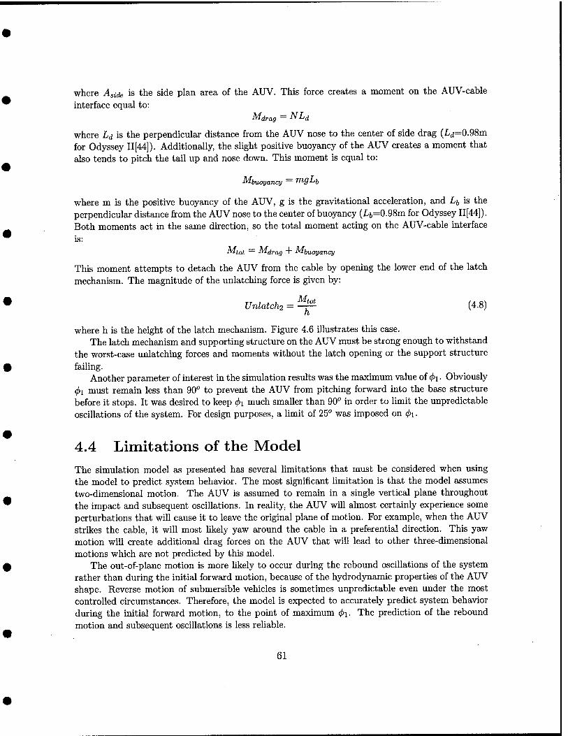
where Aside is the side plan axea of the AUV. This force creates a moment on the AUV-cable interface equal to:
Mdrag = NLd
where Ld is the perpendicular distance from the AUV nose to the center of side drag (Ld=0.98m for Odyssey II [44]). Additionally, the slight positive buoyancy of the AUV creates a moment that also tends to pitch the tail up and nose down. This moment is equal to:
^buoyancy ^^ f^QJ-'b
where m is the positive buoyancy of the AUV, g is the gravitational acceleration, and Lt is the perpendicular distance from the AUV nose to the center of buoyancy (L6=0.98m for Odyssey II[44]). Both moments act in the same direction, so the total moment acting on the AUV-cable interface is:
^tot = ^drag + M^buoyancy
This moment attempts to detach the AUV from the cable by opening the lower end of the latch mechanism. The magnitude of the unlatching force is given by:
Unlatch2 = ^ (4.8) n
where h is the height of the latch mechanism. Figure 4.6 illustrates this case. The latch mechanism and supporting structure on the AUV must be strong enough to withstand
the worst-case unlatching forces and moments without the latch opening or the support structure faihng.
Another parameter of interest in the simulation results was the maximum value of (j)i. Obviously (1)1 must remain less than 90° to prevent the AUV from pitching forward into the base structure before it stops. It was desired to keep 0i much smaller than 90° in order to limit the unpredictable oscillations of the system. For design purposes, a Umit of 25° was imposed on (j)i.
4.4 Limitations of the Model The simulation model as presented has several limitations that must be considered when using the model to predict system behavior. The most significant Umitation is that the model assumes two-dimensional motion. The AUV is assumed to remain in a single vertical plane throughout the impact and subsequent oscillations. In reality, the AUV will almost certainly experience some perturbations that will cause it to leave the original plane of motion. For example, when the AUV strikes the cable, it will most likely yaw around the cable in a preferential direction. This yaw motion will create additional drag forces on the AUV that will lead to other three-dimensional motions which are not predicted by this model.
The out-of-plane motion is more likely to occur during the rebound oscillations of the system rather than during the initial forward motion, because of the hydrodynamic properties of the AUV shape. Reverse motion of submersible vehicles is sometimes unpredictable even under the most controlled circumstances. Therefore, the model is expected to accurately predict system behavior during the initial forward motion, to the point of maximum <pi. The prediction of the rebound motion and subsequent oscillations is less reliable.
61
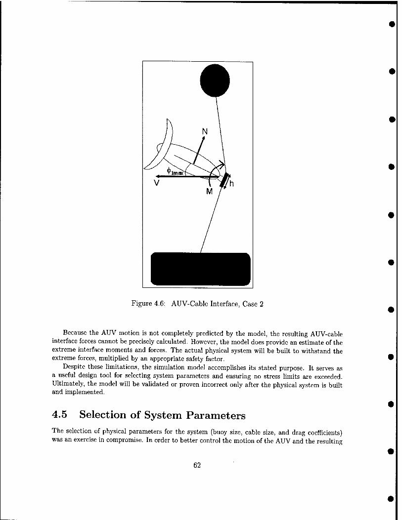
Figure 4.6: AUV-Cable Interface, Case 2
Because the AUV motion is not completely predicted by the model, the resulting AUV-cable interface forces cannot be precisely calculated. However, the model does provide an estimate of the extreme interfax;e moments and forces. The actual physical system will be built to withstand the extreme forces, multiplied by an appropriate safety factor.
Despite these hmitations, the simulation model accomplishes its stated purpose. It serves as a useful design tool for selecting system parameters and ensuring no stress limits are exceeded. Ultimately, the model will be validated or proven incorrect only after the physical system is built and implemented.
4.5 Selection of System Parameters The selection of physical parameters for the system (buoy size, cable size, and drag coefficients) was an exercise in compromise. In order to better control the motion of the AUV and the resulting
62
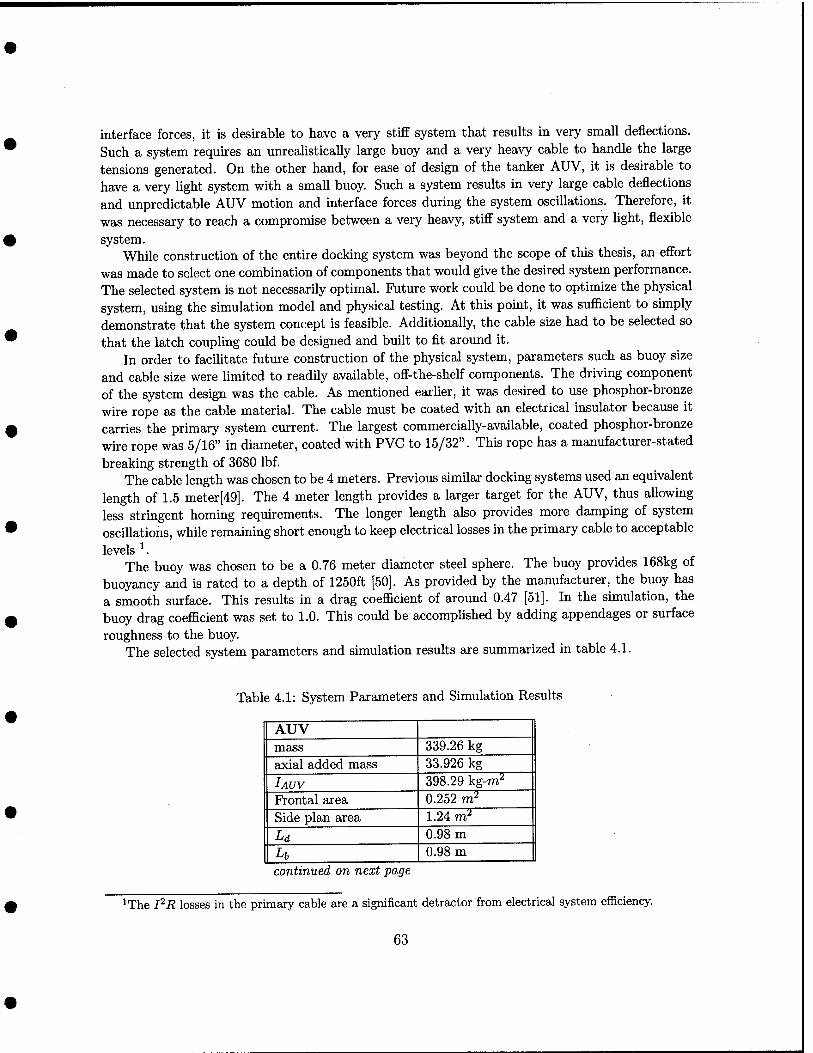
interface forces, it is desirable to have a very stiff system that results in very small deflections. Such a system requires an unrealistically large buoy and a very heavy cable to handle the large tensions generated. On the other hand, for ease of design of the tanker AUV, it is desirable to have a very light system with a small buoy. Such a system results in very large cable deflections and unpredictable AUV motion and interface forces during the system oscillations. Therefore, it was necessary to reach a compromise between a very heavy, stiff system and a very light, flexible system.
While construction of the entire docking system was beyond the scope of this thesis, an effort was made to select one combination of components that would give the desired system performance. The selected system is not necessarily optimal. Future work could be done to optimize the physical system, using the simulation model and physical testing. At this point, it was sufficient to simply demonstrate that the system concept is feasible. Additionally, the cable size had to be selected so that the latch coupling could be designed and built to fit around it.
In order to facilitate future construction of the physical system, parameters such as buoy size and cable size were hmited to readily available, off-the-shelf components. The driving component of the system design was the cable. As mentioned earlier, it was desired to use phosphor-bronze wire rope as the cable material. The cable must be coated with an electrical insulator because it carries the primary system current. The largest commercially-available, coated phosphor-bronze wire rope was 5/16" in diameter, coated with PVC to 15/32". This rope has a manufacturer-stated breaking strength of 3680 Ibf.
The cable length was chosen to be 4 meters. Previous similar docking systems used an equivalent length of 1.5 meter[49]. The 4 meter length provides a larger target for the AUV, thus allowing less stringent homing requirements. The longer length also provides more damping of system oscillations, while remaining short enough to keep electrical losses in the primary cable to acceptable levels ^.
The buoy was chosen to be a 0.76 meter diameter steel sphere. The buoy provides 168kg of buoyancy and is rated to a depth of 1250ft [50]. As provided by the manufacturer, the buoy has a smooth surface. This results in a drag coefficient of around 0.47 [51]. In the simulation, the buoy drag coefficient was set to 1.0. This could be accomplished by adding appendages or surface roughness to the buoy.
The selected system parameters and simulation results are summarized in table 4.1.
Table 4.1: System Parameters and Simulation Results
AUV mass 339.26 kg axial added mass 33.926 kg
IAUV 398.29 kg-m^ Frontal area 0.252 m^ Side plan area 1.24 m^
Ld 0.98 m
Lb 0.98 m continued on next page
^The PR losses in the primary cable are a significant detractor from electrical system efficiency.
63
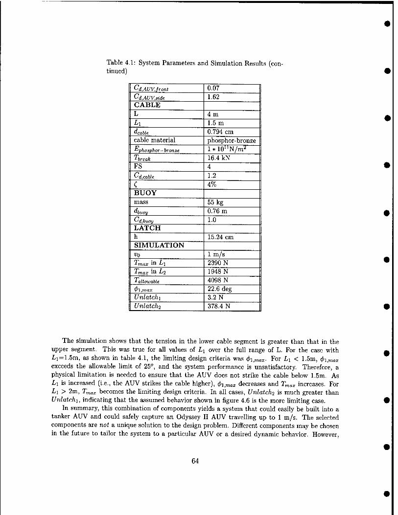
Table 4.1: System Parameters and Simulation Results (con- tinued)
Cd,AUVJront 0.07 Cd,AUV,side 1.62 CABLE L 4 m Li 1.5 m dcable 0.794 cm cable material phosphor-bronze ^phosphor—bronze 1 * WN/m'^ Tbreak 16.4 kN FS 4 Cd,cable 1.2 C 4% BUOY mass 55 kg "■buoy 0.76 m ^d,buoy 1.0 LATCH h 15.24 cm SIMULATION vo 1 m/s Tmax in Ll 2390 N Tmax in L2 1948 N -' allowable 4098 N 01,mm 22.6 deg Unlatchi 3.2 N Unlatch2 378.4 N
The simulation shows that the tension in the lower cable segment is greater than that in the upper segment. This was true for all values of Li over the full range of L. For the case with Li=1.5m, as shown in table 4.1, the limiting design criteria was (f>i^max- For Li < 1.5m, (pi^max exceeds the allowable limit of 25°, and the system performance is unsatisfactory. Therefore, a physical limitation is needed to ensure that the AUV does not strike the cable below 1.5m. As Li is increased (i.e., the AUV strikes the cable higher), 0i,mai decreases and Tmax increases. For Li > 2m, Tmax becomes the limiting design criteria. In all cases, Unlatch2 is much greater than Unlatchi, indicating that the assumed behavior shown in figure 4.6 is the more Hmiting case.
In summary, this combination of components yields a system that could easily be built into a tanker AUV and could safely capture an Odyssey II AUV travelling up to 1 m/s. The selected components are not a unique solution to the design problem. Different components may be chosen in the future to tailor the system to a particular AUV or a desired dynamic behavior. However,
64

this example system proves the utiUty of the simulation tool, and demonstrates the mechanical feasibility of the design.
4.6 Nomenclature A Ust of all terms and variables used in this chapter is shown in table 4.2.
Table 4.2: Chapter 4 Nomenclature
A area B buoyant force acting on buoy c viscous damping constant
CD drag coefficient d diameter D damping energy DOF degree of freedom e unit vector E modulus of elasticity
/e generalized force F external force FS factor of safety
g gravitational acceleration h height of latch mechanism
IAUV mass moment of inertia of the AUV about its nose
■^buoy mass moment of inertia of the buoy k linear spring constant K kinetic energy L total cable length Li lower cable section length
L2 upper cable section length
Lb distance from AUV nose to center of buoyancy
Ld distance from AUV nose to center of side drag m AUV mass M buoy mass N normal drag force on AUV
q degree of freedom R net vertical force on buoy s dummy variable indicating position along cable section T cable tension u displacement coordinate V velocity V potential or spring energy continued on next page
65
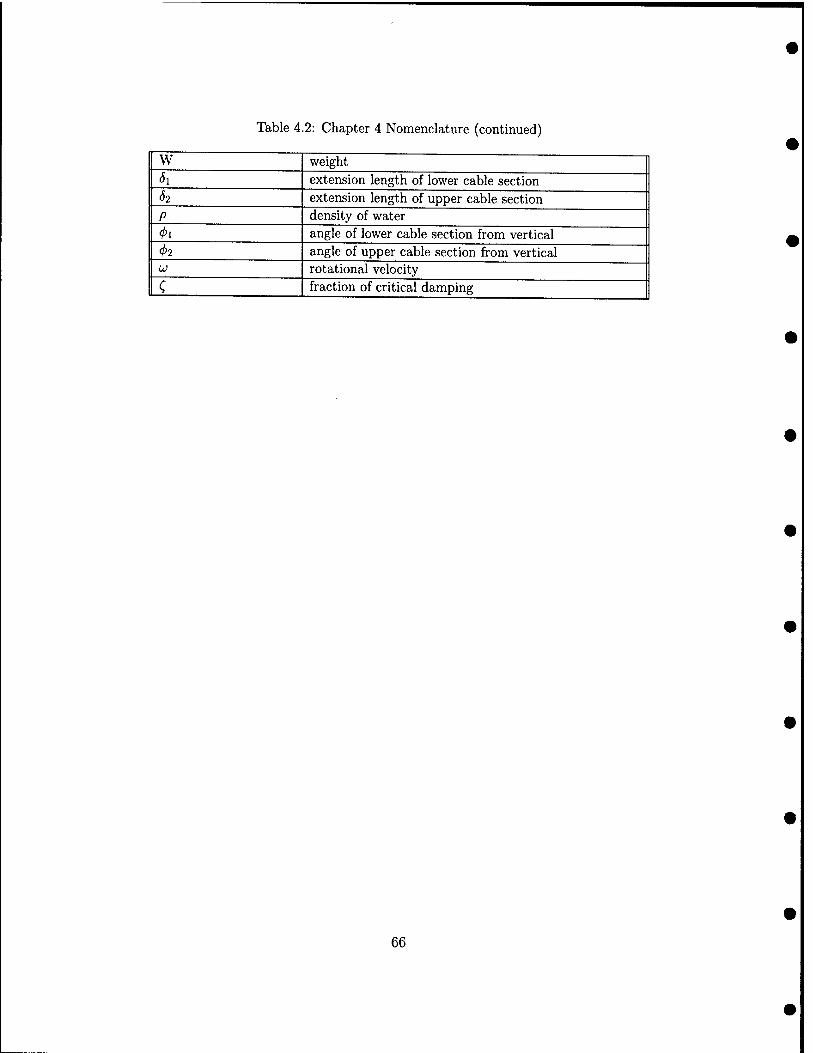
Table 4.2: Chapter 4 Nomenclature (continued)
W 6i
4>2 (jj
weight extension length of lower cable section extension length of upper cable section density of water angle of lower cable section from vertical angle of upper cable section from vertical rotational velocity fraction of critical damping
66

Chapter 5
Electrical System Design
5.1 Fundamental Theory and Background The electrical portion of the proposed AUV recharge system is based on a linear coaxial-wound transformer (LCWT) inductive coupUng. The LCWT was chosen because it allows power transfer directly between the capture wire and the latch mechanism on the AUV, without conductive contact. This allows greater mechanical design flexibility than systems using wet-mateable pin connections or inductive pucks. The capture wire is actually an insulated conductor loop through which AC current circulates. The capture wire serves as the primary winding of the transformer. The LCWT is a cylindrical magnetic core integrated into the latch mechanism on the AUV. The secondary transformer windings are wound onto the cyhndrical core. When the LCWT closes around the capture wire, a magnetic circuit is created. The AC current in the wire induces a voltage across the secondary windings, which in ttun produces a current that is fed to the AUV power electronics and eventually to the AUV battery for recharging.
LCWTs (also referred to as sliding transformers or clamp-on transformers) are presently used in several contactless power transfer applications. The most common use is in power delivery to mobile loads, such as rail vehicles like trains and gantry cranes. In this kind of application, the primary cable loop runs the length of the rail. The LCWT is mounted on the moving vehicle and encircles the primary cable. The LCWT is often gapped (i.e., not a closed cyhnder) to allow passage around cable supports. The LCWT provides contactless power transfer that is independent of the relative motion between the load and the primary cable. A second common use of LCWTs is power supphes for portable AC equipment. Rather than using conventional AC outlets and plug-in equipment, a primary cable loop is run through the area. Each piece of portable AC gear is equipped with a clamp-on LCWT. The LCWT may be clamped onto the primary cable anywhere along its length to draw power inductively. This type of system is particularly useful in harsh industrial environments because all components can be sealed in dustproof and waterproof housings, with no exposed electrical contacts [52].
The electrical system proposed here is similar to that designed by Heeres at the University of Wisconsin[53]. Heeres proposed a system of a stationary submerged primary loop and several mobile submerged loads, each with its own clamp-on LCWT. The LCWTs can connect anywhere on the primary loop to draw power. Heeres reported that a prototype 3kVA LCWT inductive coupler achieved power transfer efBciencies of 85% in salt water. However, his tests were conducted
67
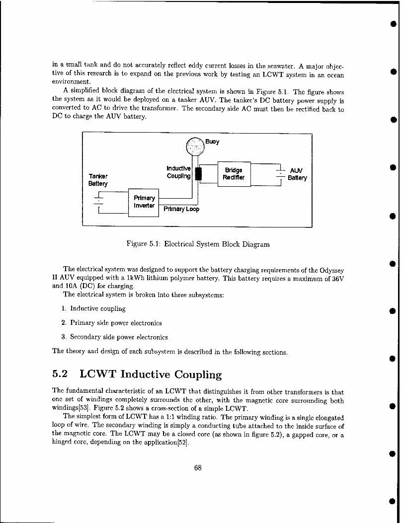
in a small tank and do not ax;curately reflect eddy current losses in the seawater. A major objec- tive of this research is to expand on the previous work by testing an LCWT system in an ocean environment.
A simplified block diagram of the electrical system is shown in Figure 5.1. The figure shows the system as it would be deployed on a tanker AUV. The tanker's DC battery power supply is converted to AC to drive the transformer. The secondary side AC must then be rectified back to DC to charge the AUV battery.
Buoy
Tanker Battery
Inductive Coupling
Primary Inverter Primary Loop
Id Bridge Rectifier
AUV Battery
Figure 5.1: Electrical System Block Diagram
The electrical system was designed to support the battery charging requirements of the Odyssey II AUV equipped with a IkWh lithium polymer battery. This battery requires a maximum of 36V and lOA (DC) for charging.
The electrical system is broken into three subsystems:
1. Inductive coupfing
2. Primary side power electronics
3. Secondary side power electronics
The theory and design of each subsystem is described in the following sections.
5.2 LCWT Inductive Coupling
The fundamental characteristic of an LCWT that distinguishes it from other transformers is that one set of windings completely surrounds the other, with the magnetic core surrounding both windings[53]. Figure 5.2 shows a cross-section of a simple LCWT.
The simplest form of LCWT has a 1:1 winding ratio. The primary winding is a single elongated loop of wire. The secondary winding is simply a conducting tube attached to the inside surface of the magnetic core. The LCWT may be a closed core (as shown in figure 5.2), a gapped core, or a hinged core, depending on the application[52].
68
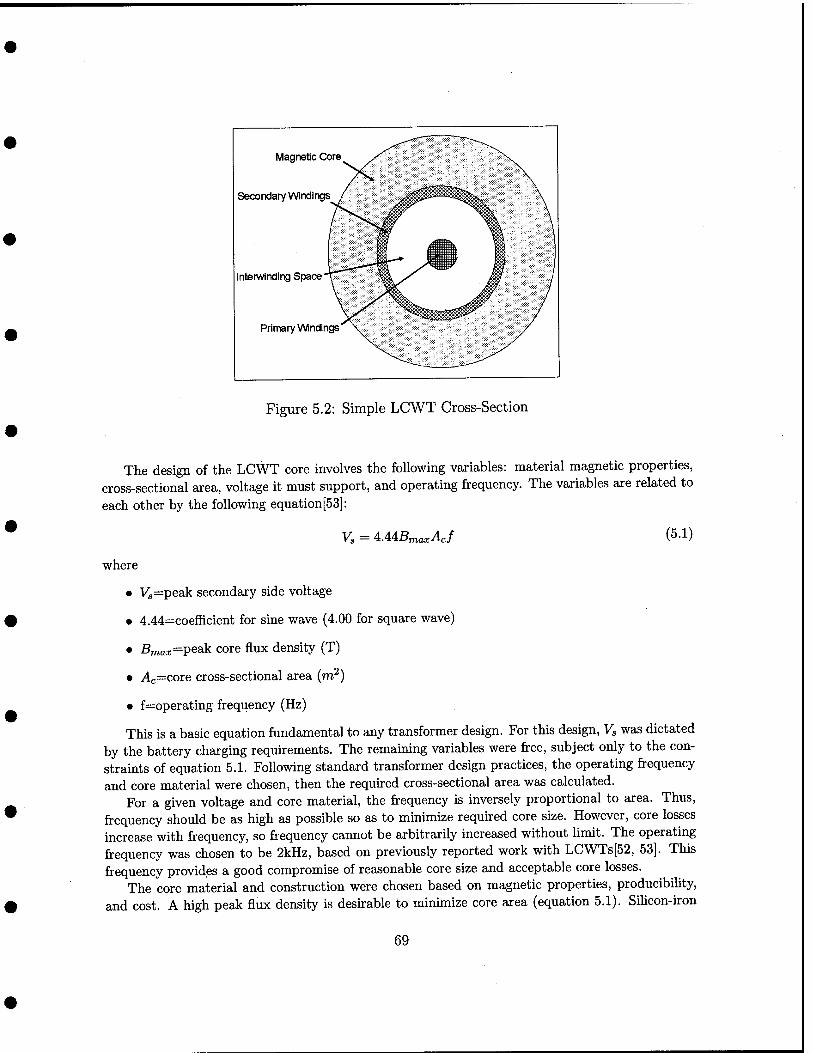
Magnetic Core
Secondary Windings
Intetwinding Space
Primary Windings
Figure 5.2: Simple LCWT Cross-Section
The design of tlie LCWT core involves the following variables: material magnetic properties, cross-sectional area, voltage it must support, and operating frequency. The variables are related to each other by the following equation[53]:
V, = ^AAB^axAcf (5.1)
where
• V's=peak secondary side voltage
• 4.44=coefficient for sine wave (4.00 for square wave)
• Bmax—V^^ core flux density (T)
• Ac=core cross-sectional area {vn?)
• f=operating frequency (Hz)
This is a basic equation fundamental to any transformer design. For this design, Vs was dictated by the battery charging requirements. The remaining variables were free, subject only to the con- straints of equation 5.1. Following standard transformer design practices, the operating frequency and core material were chosen, then the required cross-sectional area was calculated.
For a given voltage and core material, the frequency is inversely proportional to area. Thus, frequency should be as high as possible so as to minimize required core size. However, core losses increase with frequency, so frequency cannot be arbitrarily increased without limit. The operating frequency was chosen to be 2kHz, based on previously reported work with LCWTs[52, 53]. This frequency provides a good compromise of reasonable core size and acceptable core losses.
The core material and construction were chosen based on magnetic properties, producibihty, and cost. A high peak flux density is desfrable to minimize core area (equation 5.1). Silicon-iron
69
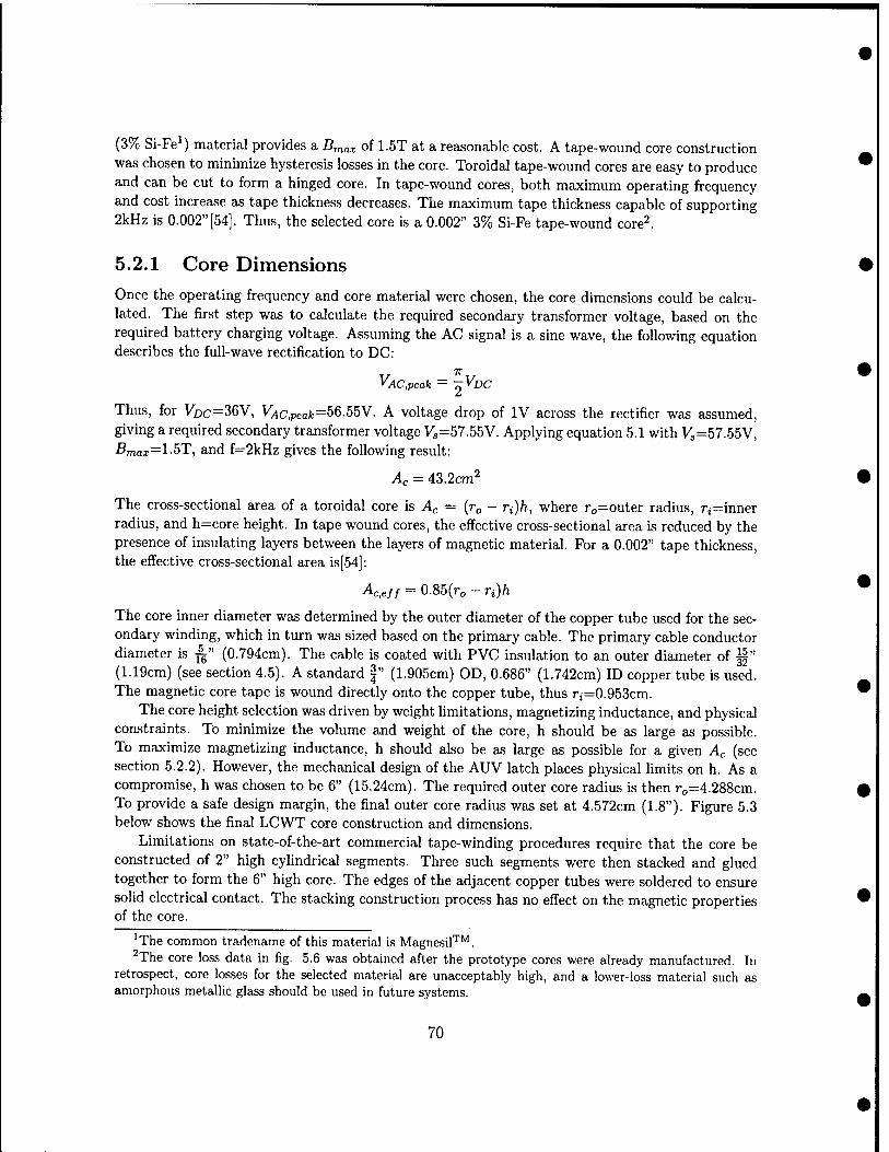
(3% Si-Fe') material provides a Bmax of 1.5T at a reasonable cost. A tape-wound core construction was chosen to minimize hysteresis losses in the core. Toroidal tape-wound cores are easy to produce and can be cut to form a hinged core. In tape-wound cores, both maximum operating frequency and cost increase as tape thickness decreases. The maximum tape thickness capable of supporting 2kHz is 0.002" [54]. Thus, the selected core is a 0.002" 3% Si-Fe tape-wound core^.
5.2.1 Core Dimensions Once the operating frequency and core material were chosen, the core dimensions could be calcu- lated. The first step was to calculate the required secondary transformer voltage, based on the required battery charging voltage. Assuming the AC signal is a sine wave, the following equation describes the full-wave rectification to DC:
Thus, for Vbc=36V, Vyic,peafc=56.55V. A voltage drop of IV across the rectifier was assumed, giving a required secondary transformer voltage V;=57.55V. Applying equation 5.1 with Vs=57.55V, •Bmax=l-5T, and f=2kHz gives the following result:
Ac = 43.2cm2
The cross-sectional area of a toroidal core is A^ = {TQ - ri)h, where ro=outer radius, ri=inner radius, and h=core height. In tape wound cores, the effective cross-sectional area is reduced by the presence of insulating layers between the layers of magnetic material. For a 0.002" tape thickness, the effective cross-sectional area is[54]:
Ac^eff = 0.85(ro - ri)h
The core inner diameter was determined by the outer diameter of the copper tube used for the sec- ondary winding, which in turn was sized based on the primary cable. The primary cable conductor diameter is ^" (0.794cm). The cable is coated with PVC insulation to an outer diameter of i|" (1.19cm) (see section 4.5). A standard f" (1.905cm) OD, 0.686" (1.742cm) ID copper tube is used. The magnetic core tape is wound directly onto the copper tube, thus ri=0.953cm.
The core height selection was driven by weight limitations, magnetizing inductance, and physical constraints. To minimize the volume and weight of the core, h should be as large as possible. To maximize magnetizing inductance, h should also be as large as possible for a given Ac (see section 5.2.2). However, the mechanical design of the AUV latch places physical limits on h. As a compromise, h was chosen to be 6" (15.24cm). The required outer core radius is then ro=4.288cm. To provide a safe design margin, the final outer core radius was set at 4.572cm (1.8"). Figure 5.3 below shows the final LCWT core construction and dimensions.
Limitations on state-of-the-art commercial tape-winding procedures require that the core be constructed of 2" high cylindrical segments. Three such segments were then stacked and glued together to form the 6" high core. The edges of the adjacent copper tubes were soldered to ensure solid electrical contact. The stacking construction process has no effect on the magnetic properties of the core.
'The common tradename of this material is MagnesiF'^. ^The core loss data in fig. 5.6 was obtained after the prototype cores were already manufactured. In
retrospect, core losses for the selected material are unacceptably high, and a lower-loss material such as amorphous metallic glass should be used in future systems.
70
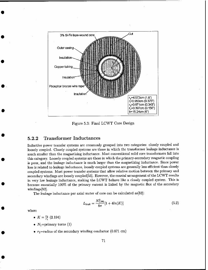
3% Si-Fe tape-wound core CXit
Insulal -^s^a^g^Sjac*- r„=4.572cm(1.8")
rpO. 953cm (0.375") r2=0.871cm (0.343") ri=0.397cm (0.156") h=15.24cm (6")
Figure 5.3: Final LCWT Core Design
5.2.2 Transformer Inductances Inductive power transfer systems are commonly grouped into two categories: closely coupled and loosely coupled. Closely coupled systems are those in which the transformer leakage inductance is much smaller than the magnetizing inductance. Most conventional sohd core transformers fall into this category. Loosely coupled systems are those in which the primary-secondary magnetic coupUng is poor, and the leakage inductance is much larger than the magnetizing inductance. Since power loss is related to leakage inductance, loosely coupled systems are generally less efficient than closely coupled systems. Most power transfer systems that allow relative motion between the primary and secondary windings are loosely coupled[55]. However, the coaxial arrangement of the LCWT results in very low leakage inductance, making the LCWT behave like a closely coupled system. This is because essentially 100% of the primary current is Unked by the magnetic flux of the secondary windings [52].
The leakage inductance per axial meter of core can be calculated as[52]:
Lleak 8n [1 + 4ln{K)] (5.2)
where
• K = ^f^ (2.194)
• A/'i=primary turns (1)
• r2=radius of the secondary winding conductor (0.871 cm)
71
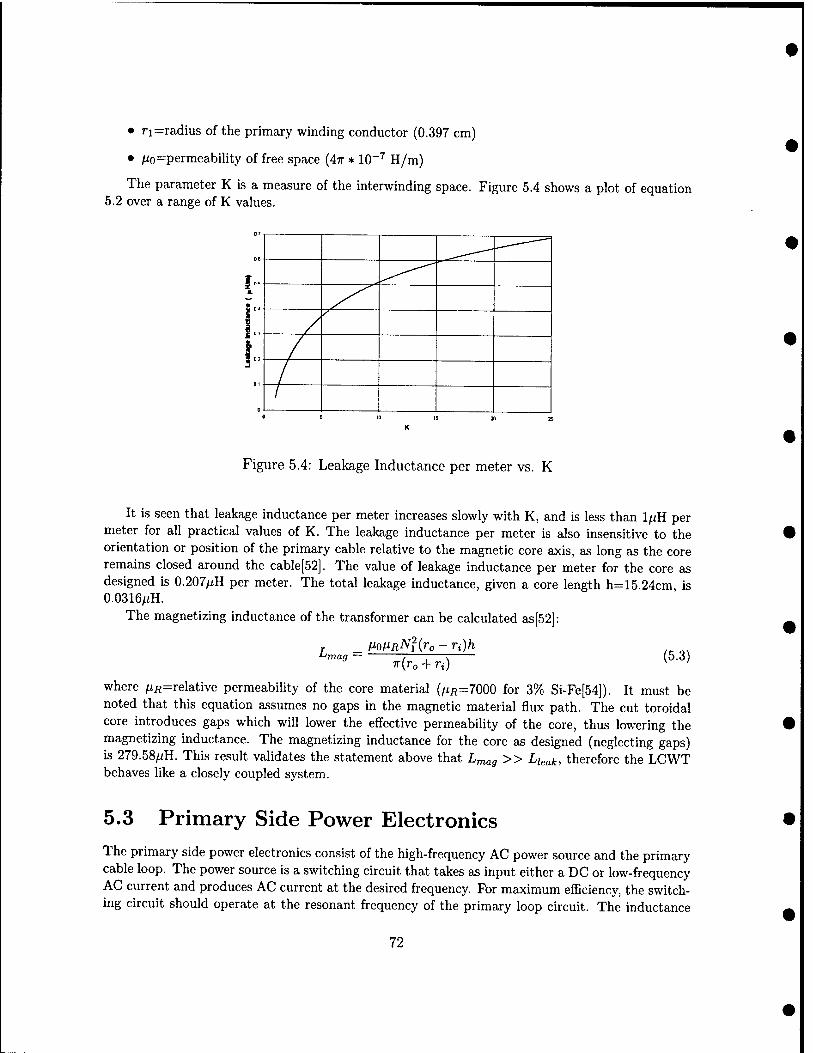
• ri=radius of the primary winding conductor (0.397 cm)
• /xo=permeability of free space {4n * 10"''' H/m)
The parameter K is a measure of the interwinding space. Figure 5.4 shows a plot of equation 5.2 over a range of K values.
Figure 5.4: Leakage Inductance per meter vs. K
It is seen that leakage inductance per meter increases slowly with K, and is less than l^H per meter for all practical values of K. The leakage inductance per meter is also insensitive to the orientation or position of the primary cable relative to the magnetic core axis, as long as the core remains closed around the cable [52]. The value of leakage inductance per meter for the core as designed is 0.207/iH per meter. The total leakage inductance, given a core length h=15.24cm, is 0.0316MH.
The magnetizing inductance of the transformer can be calculated as [52]:
-'mag _ MoMfl-^^?(^o -ri)h
7r(rc, + rj) (5.3)
where ^^^relative permeability of the core material (/x/{=7000 for 3% Si-Fe[54]). It must be noted that this equation assumes no gaps in the magnetic material flux path. The cut toroidal core introduces gaps which will lower the effective permeability of the core, thus lowering the magnetizing inductance. The magnetizing inductance for the core as designed (neglecting gaps) is 279.58/iH. This result validates the statement above that Lmag » Lieak, therefore the LCWT behaves like a closely coupled system.
5.3 Primary Side Power Electronics The primary side power electronics consist of the high-frequency AC power source and the primary cable loop. The power source is a switching circuit that takes as input either a DC or low-frequency AC current and produces AC current at the desired frequency. For maximum efficiency, the switch- ing circuit should operate at the resonant frequency of the primary loop circuit. The inductance
72
of the primary cable loop is compensated with a parallel or series capacitor at the inverter output. This minimizes the reactive power drawn by the system. The power source will typically supply a constant current to the primary loop, letting the voltage vary as a function of the load [55]. Detailed design of a switching circuit and compensation is beyond the scope of this research, and is left as future work; examples of such designs may be found in the literature[52, 53, 55, 56]. However, it must be noted that the power source design is critical to the overall eflBciency of the inductive power transfer system.
The primary cable loop itself has both inductance and resistance. The inductance of the loop may be calculated as [52]:
where D=lateral spacing between the primary cable segments and l=loop length. Assuming a lateral spacing D=5cm and loop length l=4m, Lioop = 4.054/xH. Equation 5.4 indicates that primary loop inductance is insensitive to cable size or lateral spacing, but is hnearly dependent on cable length.
The primary cable loop resistance may be calculated as [56]:
t^loop — 21 (5.5)
where o-c=material conductivity and Ap=conductor cross-sectional area. For the phosphor-bronze wire rope used as the primary cable in this design, dc -= 1.94 * 10^ j^ and Ap = 0.255cm2. The resulting loop resistance is: Rioop = 16.17mn.
The primary loop inductance and resistance may be combined with the leakage inductance and magnetizing inductance calculated above to create an equivalent circuit for the loop and LCWT, as shown in figure 5.5.
•
AC SOURCE
R|oop
R„,p=16.17mfi L|OOP=4.054AH
L|eak=0.0316^H Lmao=279.58^H
A/ OOP Heak
\AA AAAA
i
^mag LOAD
• 1
Figure 5.5: Equivalent Circuit of Primary Loop and LCWT
73
The circuit is asymmetric because there is no leakage inductance on the secondary side. As discussed above, the primary current is completely linked by the magnetic flux of the secondary winding, but not vice versa[52].
5.4 Secondary Side Power Electronics
The secondary side power electronics consist of the secondary windings and power leads, a bridge rectifier and filter to convert the high-frequency AC signal to DC, and any other power conditioning circuits specific to the load. The design of the secondary side converter is beyond the scope of this research and is left as future work. Specific secondary side converter topologies and compensation schemes may be found in the literature[52, 55].
The resistance of the copper tube secondary winding may be calculated as:
For the given tubing size (OD=1.905cm, ID-1.742cm), Rcu = 5.628*10-^0. The power leads that run from the secondary winding to the converter are assumed to be twisted together (or coaxial) and as short as possible to minimize secondary loop inductance. On the Odyssey II AUV, the secondary power leads will be less than Im in length.
The battery charging control circuitry could be located on either the primary or secondary side of the system. Prom a weight and volume perspective, it is advantageous to locate the circuitry on the primary side (i.e., in the tanker AUV or dock base) rather than on the secondary side (i.e., in the AUV). The docking station could then receive an identifying acoustic signal from the docked AUV and provide charging power tailored to that specific AUV.
5.5 System Losses and Efficiency
The power losses that affect the inductive power transfer system may be categorized as follows:
1. Ohmic (/^i?) losses
2. Hysteresis losses in the core
3. Eddy current losses
4. Leakage and loop inductance losses
This discussion considers only the losses in the system components between (but not including) the primary and secondary side converters. This corresponds to the efficiencies measured during experimentation (see Chapter 6).
The ohmic power loss of the entire system is dominated by losses in the primary cable loop [52]. The primary cable losses may be written as:
^cable — I V2j Ri oop
74
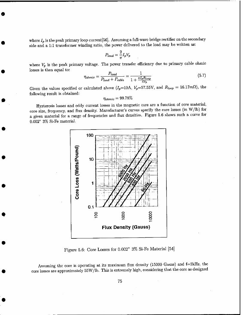
where Ip is the peak primary loop current [56]. Assuming a full-wave bridge rectifier on the secondary side and a 1:1 transformer winding ratio, the power delivered to the load may be written as:
2 Pload — ~J-pyp
IT
where Vp is the peak primary voltage. The power transfer efficiency due to primary cable ohmic losses is then equal to:
— "load }^ eg y") Vohmic - p^^^^ ^ p^^^^ - ^ ^ w^
Given the values specified or calculated above (/p^lOA, yp=57.55V, and Rioap = 16.17mf2), the following result is obtained:
riohmic = 99.78%
Hysteresis losses and eddy current losses in the magnetic core are a function of core material, core size, frequency, and flux density. Manufacturer's curves specify the core losses (in W/lb) for a given material for a range of frequencies and flux densities. Figure 5.6 shows such a curve for 0.002" 3% Si-Fe material.
Figure 5.6: Core Losses for 0.002" 3% Si-Fe Material [54]
core
Assuming the core is operating at its maximum flux density (15000 Gauss) and f-2kHz, the losses are approximately 55W/lb. This is extremely high, considering that the core as designed
75
weighs 16.111b. The total core losses (at peak power) are then equal to 886W. The power transfer efficiency due to core losses is then equal to:
■• load I .» core
For the values given, r}core = 28.89%. This efficiency could be significantly improved through the use of lower-loss core material, such as amorphous metallic glass.
Since this system will operate in conductive saltwater, eddy currents will be generated in the surrounding water as well as in the core. Heeres published a theoretical analysis of the seawater eddy current effects[53]. The seawater introduces an additional impedance, given by:
where
• C = \/j27r//ioMfiCTsu,
• /i'o,/^i=modified Bessel functions
• asuj=conductivity of seawater
Ekjuation 5.9 indicates that the seawater impedance is a function of the lateral spacing between the primary conductor segments, D. The seawater impedance is equal to 0 when D=ri, and increases as D increases. This result suggests that the primary cable separation should be as small as physically possible to minimize power losses in the seawater. This is because eddy currents tend to concentrate in the first skin depth of a material. Skin depth is given by the equation:
For f=2kHz, the seawater skin depth is equal to 5.63m. If the two primary conductor segments are within one skin depth of each other, the magnetic fields and resulting eddy currents generated by the two segments will cancel each other everywhere except in the small region between the conductors. The effect of lateral spacing on power transfer efficiency was investigated experimentally with the prototype core, and is discussed in section 6.4.
The losses due to the leakage and loop inductances are not real power losses per se, and will not affect power transfer efficiency directly. Rather, they are reactive power penalties. If the loop and leakage inductances are compensated with a capacitor, as discussed in section 5.3, then reactive energy will oscillate between the inductance and capacitance. The reactive energy that oscillates per cycle may be written as:
^r = Izi.Lieak + Lioop)Ip
The energy delivered to the load per cycle may be written as:
_ 2IpVp load t Wlo ■ - -^'^
76
The system penalty factor is then defined as:
r — ^^ — ^/-^p(-^^eofc + Lioop) /c ii\
For the given system parameters, Tg = 0.0562%. While Tg does not indicate real power losses, it does affect the required primary side voltage, which in turn affects other system power losses. Therefore, it is desirable to minimize rs[56].
77

This page intentionally blank
78
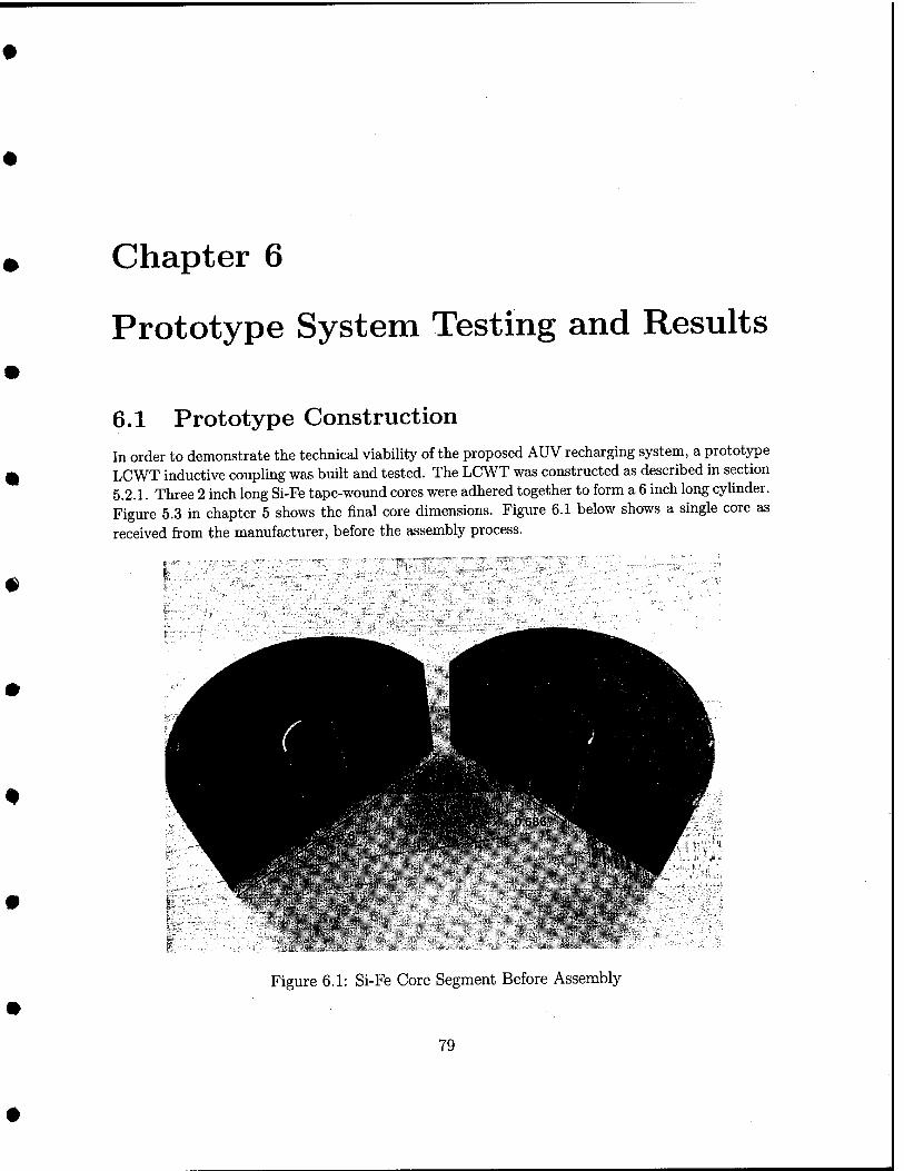
Chapter 6
Prototype System Testing and Results
6.1 Prototype Construction In order to demonstrate the technical viabiUty of the proposed AUV recharging system, a prototype LCWT inductive coupling was built and tested. The LCWT was constructed as described in section 5.2.1. Three 2 inch long Si-Fe tape-wound cores were adhered together to form a 6 inch long cyUnder. Figure 5.3 in chapter 5 shows the final core dimensions. Figure 6.1 below shows a single core as received from the manufacturer, before the assembly process.
> , ... :» ■••
Figure 6.1: Si-Fe Core Segment Before Assembly
79

The core segments were bonded together using West System two part marine epoxy. After the three core segments were connected, the edges of the adjacent copper tubing sections were joined with 3M conducting adhesive copper tape to ensure sohd electrical contact. The two semi-cyhnders were then electrically joined by soldering a jumper cable between the copper tubes on either end. Additionally, power leads were soldered to each end of one of the copper tubing sections. The two power leads were then combined via a Y-splice into a single waterproof two conductor cable leading to the load. Figure 6.2 shows the two semi-cylinders with the jumper cable and power lead being attached to the first end.
#
Figure 6.2: Core Segments During Assembly
Following the attachment of all leads and verification of electrical continuity, the entire core assembly was encapsulated to waterproof it. First, the inner core faces and copper tubing were painted with marine epoxy to create a thin (about 1 mm) waterproof seal. Then the outer core surfaces and cable ends were coated with 3M Scotchcast"^". The Scotchcast'^'^'sealed as well as strengthened the entire core assembly. Figure 6.3 shows the completed core assembly, the Y-splice, and the power cable.
80
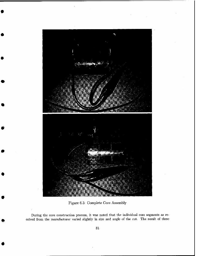
Figure 6.3: Complete Core Assembly
During the core construction process, it was noted that the individual core segments as re- ceived from the manufacturer varied slightly in size and angle of the cut. The result of these
81
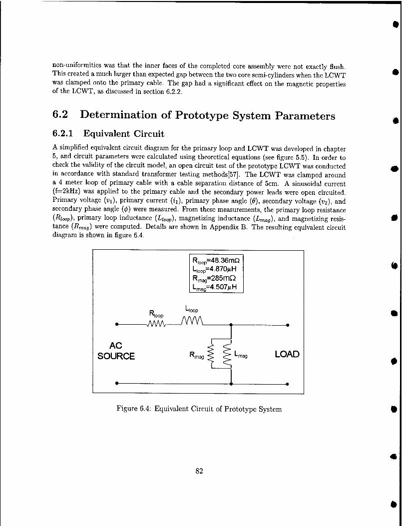
non-uniformities was that the inner faces of the completed core assembly were not exactly flush. This created a much larger than expected gap between the two core semi-cylinders when the LCWT was clamped onto the primary cable. The gap had a significant effect on the magnetic properties of the LCWT, as discussed in section 6.2.2.
6.2 Determination of Prototype System Parameters
6.2.1 Equivalent Circuit
A simplified equivalent circuit diagram for the primary loop and LCWT was developed in chapter 5, and circuit parameters were calculated using theoretical equations (see figure 5.5). In order to check the validity of the circuit model, an open circuit test of the prototype LCWT was conducted in accordance with standard transformer testing methods[57]. The LCWT was clamped around a 4 meter loop of primary cable with a cable separation distance of 5cm. A sinusoidal current (f=2kHz) was applied to the primary cable and the secondary power leads were open circuited. Primary voltage (DI), primary current (zi), primary phase angle ((9), secondary voltage (^2), and secondary phase angle (0) were measured. From these measurements, the primary loop resistance (Rioop), primary loop inductance (Lioop), magnetizing inductance (Lmag), and magnetizing resis- tance {Rmag) wcrc computed. Details are shown in Appendix B. The resulting equivalent circuit diagram is shown in figure 6.4.
•
AC SOURCE
f^loop
-WWv-
°loop'
'-loop"
f^mag
'-mag"
=48.36mQ =4.870MH
=285mQ =4.507^H
N OOP
Lm 39 LOAD '^mag 1 1
Figure 6.4: Equivalent Circuit of Prototype System
82
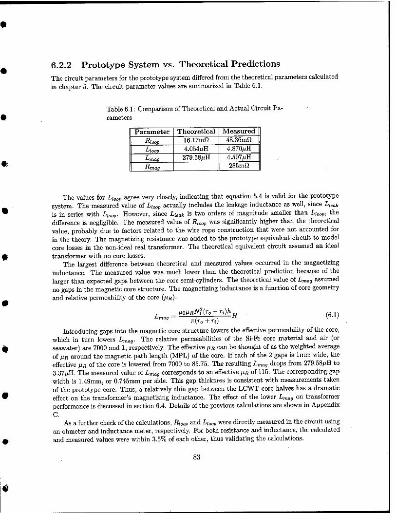
6.2.2 Prototype System vs. Theoretical Predictions The circuit parameters for the prototype system differed from the theoretical parameters calculated in chapter 5. The circuit parameter values are summarized in Table 6.1.
Table 6.1: Comparison of Theoretical and Actual Circuit Pa- rameters
Parameter Theoretical Measured
Rloop 16.17mn 48.36mfi
Lloop 4.054/iH 4.870/iH
^raag 279.58/iH 4.507MH
t(-vnag 285mf)
The values for Lioap agree very closely, indicating that equation 5.4 is valid for the prototype system. The measured value of Lioop actually includes the leakage inductance as well, since Ueak is in series with Lioap. However, since Luak is two orders of magnitude smaller than Lioop, the difference is negligible. The measured value of Rioap was significantly higher than the theoretical value, probably due to factors related to the wire rope construction that were not accounted for in the theory. The magnetizing resistance was added to the prototype equivalent circuit to model core losses in the non-ideal real transformer. The theoretical equivalent circuit assumed an ideal transformer with no core losses.
The largest diflFerence between theoretical and measured values occurred in the magnetizing inductance. The measured value was much lower than the theoretical prediction because of the larger than expected gaps between the core semi-cylinders. The theoretical value of Lmag assumed no gaps in the magnetic core structure. The magnetizing inductance is a function of core geometry and relative permeabihty of the core {HR).
'-'mag — fJ-om^K^o - ri)h H (6.1)
7r(ro -I- n) Introducing gaps into the magnetic core structure lowers the effective permeability of the core,
which in turn lowers L^ag- The relative permeabilities of the Si-Fe core material and air (or seawater) are 7000 and 1, respectively. The effective fiR can be thought of as the weighted average of HR around the magnetic path length (MPL) of the core. If each of the 2 gaps is 1mm wide, the effective JIR of the core is lowered from 7000 to 85.75. The resulting Lmag drops from 279.58/xH to 3.37/xH. The measured value of Lmag corresponds to an effective HR of 115. The corresponding gap width is 1.49mm, or 0.745mm per side. This gap thickness is consistent with measurements taken of the prototype core. Thus, a relatively thin gap between the LCWT core halves has a dramatic effect on the transformer's magnetizing inductance. The effect of the lower Lmag on transformer performance is discussed in section 6.4. Details of the previous calculations are shown in Appendix C.
As a further check of the calculations, Rioop and Lioop were directly measured in the circuit using an ohmeter and inductance meter, respectively. For both resistance and inductance, the calculated and measured values were within 3.5% of each other, thus validating the calculations.
83
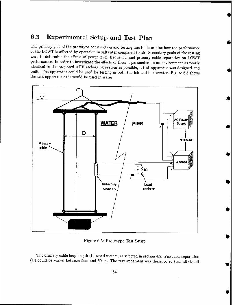
6.3 Experimental Setup and Test Plan The primary goal of the prototype construction and testing was to determine how the performance of the LCWT is affected by operation in saltwater compared to air. Secondary goals of the testing were to determine the effects of power level, frequency, and primary cable separation on LCWT performance. In order to investigate the effects of these 4 parameters in an environment as nearly identical to the proposed AUV recharging system as possible, a test apparatus was designed and built. The apparatus could be used for testing in both the lab and in seawater. Figure 6.5 shows the test apparatus as it would be used in water.
SL
Primary cable
+ ,-v AC Power
Supply
120VAC
O-scope
Load resistor
Figure 6.5: Prototype Test Setup
The primary cable loop length (L) was 4 meters, as selected in section 4.5. The cable separation (D) could be varied between 5cm and 50cm. The test apparatus was designed so that all circuit
84
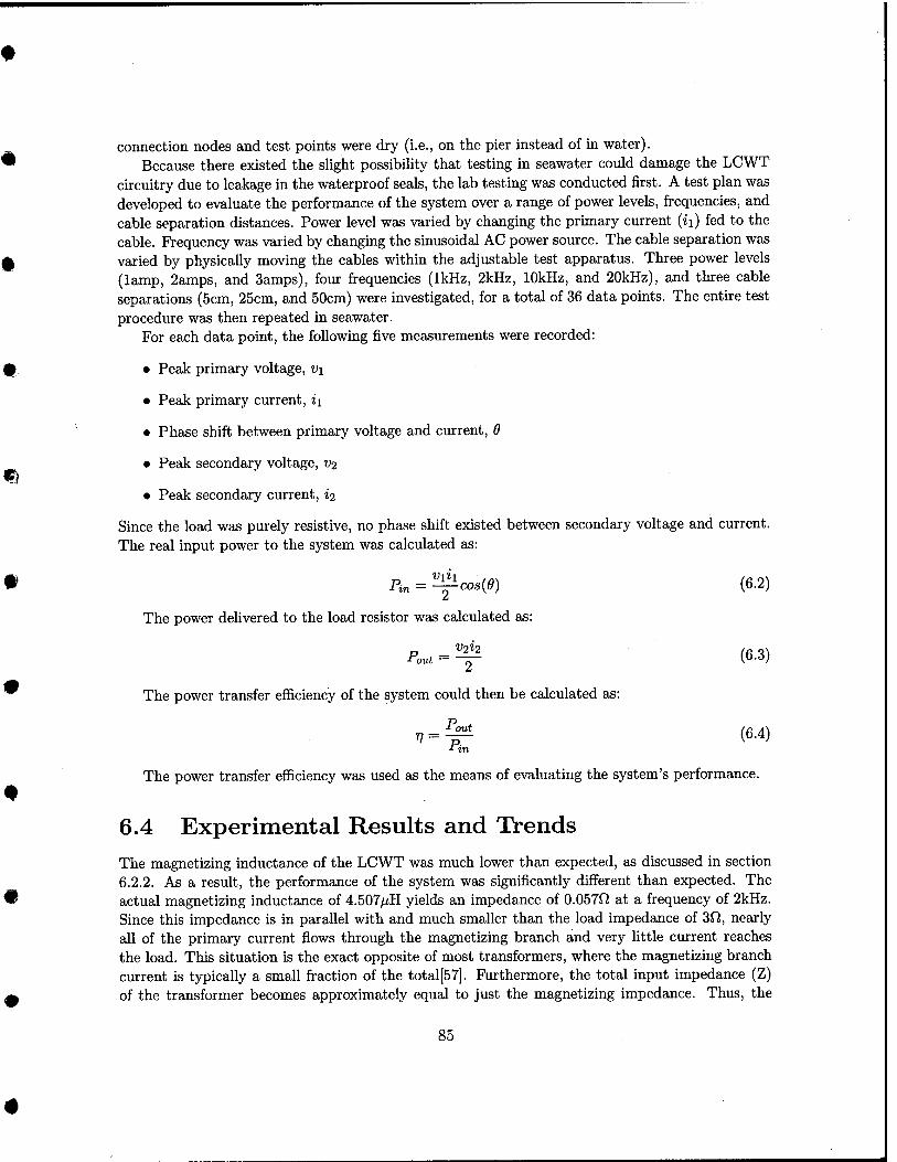
connection nodes and test points were dry (i.e., on the pier instead of in water). Because there existed the sUght possibihty that testing in seawater could damage the LCWT
circuitry due to leakage in the waterproof seals, the lab testing was conducted first. A test plan was developed to evaluate the performance of the system over a range of power levels, frequencies, and cable separation distances. Power level was varied by changing the primary current (zi) fed to the cable. Frequency was varied by changing the sinusoidal AC power source. The cable separation was varied by physically moving the cables within the adjustable test apparatus. Three power levels (lamp, 2amps, and 3amps), four frequencies (IkHz, 2kHz, lOkHz, and 20kHz), and three cable separations (5cm, 25cm, and 50cm) were investigated, for a total of 36 data points. The entire test procedure was then repeated in seawater.
For each data point, the following five measurements were recorded:
• Peak primary voltage, vi
• Peak primary current, ii
• Phase shift between primary voltage and current, 6
• Peak secondary voltage, V2
• Peak secondary current, 12
Since the load was purely resistive, no phase shift existed between secondary voltage and current. The real input power to the system was calculated as:
2 The power delivered to the load resistor was calculated as:
Pin = ^cos{e) (6.2)
Pout = -y- (6-3)
The power transfer efficiency of the system could then be calculated as:
V = §^ (6-4)
The power transfer efficiency was used as the means of evaluating the system's performance.
6.4 Experimental Results and Trends The magnetizing inductance of the LCWT was much lower than expected, as discussed in section 6.2.2. As a result, the performance of the system was significantly different than expected. The actual magnetizing inductance of 4.507/iH yields an impedance of 0.057O at a frequency of 2kHz. Since this impedance is in parallel with and much smaller than the load impedance of 3J1, nearly all of the primary current flows through the magnetizing branch and very Uttle current reaches the load. This situation is the exact opposite of most transformers, where the magnetizing branch current is typically a small fraction of the total[57]. Furthermore, the total input impedance (Z) of the transformer becomes approximately equal to just the magnetizing impedance. Thus, the
85
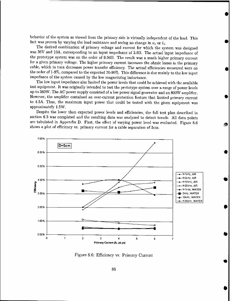
behavior of the system as viewed from the primary side is virtually independent of the load. This fact was proven by varying the load resistance and seeing no change in i;i or zi.
The desired combination of primary voltage and current for which the system was designed was 36V and lOA, corresponding to an input impedance of 3.6f). The actual input impedance of the prototype system was on the order of OMCt. The result was a much higher primary current for a given primary voltage. The higher primary current increases the ohmic losses in the primary cable, which in turn decreases power transfer efficiency. The actual efficiencies measured were on the order of 1-9%, compared to the expected 70-90%. This difference is due mainly to the low input impedance of the system caused by the low magnetizing inductance.
The low input impedance also limited the power levels that could be achieved with the available test equipment. It was originally intended to test the prototype system over a range of power levels up to 360W. The AC power supply consisted of a low power signal generator and an 800W amplifier. However, the amplifier contained an over-current protection feature that limited primary current to 4.5A. Thus, the maximum input power that could be tested with the given equipment was approximately 1.5W.
Despite the lower than expected power levels and efficiencies, the full test plan described in section 6.3 was completed and the resulting data was analyzed to detect trends. All data points are tabulated in Appendix D. First, the effect of varying power level was evaluated. Figure 6.6 shows a plot of efficiency vs. primary current for a cable separation of 5cm. i^
7.00%
6.00%
500%
S •5
4.00%
3.00%
2.00%
1.00%
0 00%
-f=1kHz,AiR -f=2kHz,AlR
-f=10kHz.AlR
-f=20kHz.AlR -f=1 kHz, WATER
-2kHz, WATER -10kHz, WATER -f=20kHz, WATER
H 3 4
Primacy Current (A, pk-pk)
Figure 6.6: Efficiency vs. Primary Current
86
No clear trends were evident in figure 6.6. This indicates that, over the power range investigated, efficiency is not a predictable function of power level. At higher power levels where core losses become significant, it is expected that efficiency will decrease as power level increases (see section
5.5). Next, the effect of frequency on efficiency was investigated. Figure 6.7 shows a plot of efficiency
vs. frequency for a 6A pk-pk primary current. This plot exhibits some noticeable trends. In air, the efficiency is maximum at f=10kHz for all values of D. In water, the maximum efficiency occurs at f=2kHz for all values of D. This difference may be due to the eddy current effect in the seawater, which is more prominent at higher frequencies. At higher power levels, it is expected that efficiency would be maximum at 2kHz, then drop sharply with higher frequencies because of the core loss properties of Si-Fe (see figure 5.6).
9.00%
8.00%
1.00%
0.00%
-D=5cm,AIR -D=25cm,AIR
-D=50cm.AIR -D=5cm, WATER -D=25cm, WATER
-D=50cm, WATER
5000 10000 15000
Frequency (Hz)
20000 25000
Figure 6.7: Efficiency vs. Frequency
Next, the effect of cable spacing on efficiency was investigated. Figure 6.8 shows a plot of efficiency vs. primary cable separation for a 6A pk-pk primary current. The data indicates that in air, the maximum efficiency occurs at D=5cm. In water, the maximum efficiency occurs at D=5o'cm. This result is unexpected based on the theory of eddy current losses in the seawater. The theory predicts that efficiency in water should be maximum at D=5cm, since eddy current losses decrease as D decreases[53].
Finally, the system efficiencies in air and water were compared. At the lower frequencies (IkHz and 2kHz)| the efficiency in water was slightly higher. At higher frequencies (lOkHz and 20kHz),
87
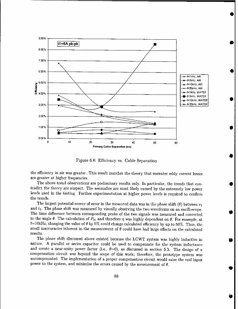
9.00%
8.00%
7.00%
1.00%
0.00%
-MkHz.AIR -f=2kHz,AIR -f=10kHz,AIR
-f=20kHz,AIR
-f=1kHz. WATER
-f=2kHz. WATER
-f=10kHz, WATER
-^20kHz, WATER
10 20 30 40
Primacy Cable Separation (cm)
50 60
Figure 6.8: Efficiency vs. Cable Separation
the efficiency in air was greater. This result matches the theory that seawater eddy current losses are greater at higher frequencies.
The above trend observations are preliminary results only. In particular, the trends that con- tradict the theory are suspect. The anomalies are most likely caused by the extremely low power levels used in the testing. Further experimentation at higher power levels is required to confirm the trends.
The largest potential source of error in the measured data was in the phase shift {6) between vi and ii. The phase shift was measured by visually observing the two waveforms on an oscilloscope. The time difference between corresponding peaks of the two signals was measured and converted to the angle 9. The calculation of Pin and therefore r] was highly dependent on 6. For example, at f=10kHz, changing the value of e by 5% could change calculated efficiency by up to 50%. Thus, the small inaccuracies inherent in the measurement of 0 could have had large effects on the calculated results.
The phase shift discussed above existed because the LCWT system was highly inductive in nature. A parallel or series capacitor could be used to compensate for the system inductance and create a near-unity power factor (i.e., 6=0), as discussed in section 5.3. The design of a compensation circuit was beyond the scope of this work; therefore, the prototype system was uncompensated. The implementation of a proper compensation circuit would raise the real input power to the system, and minimize the errors caused by the measurement of 6.
88
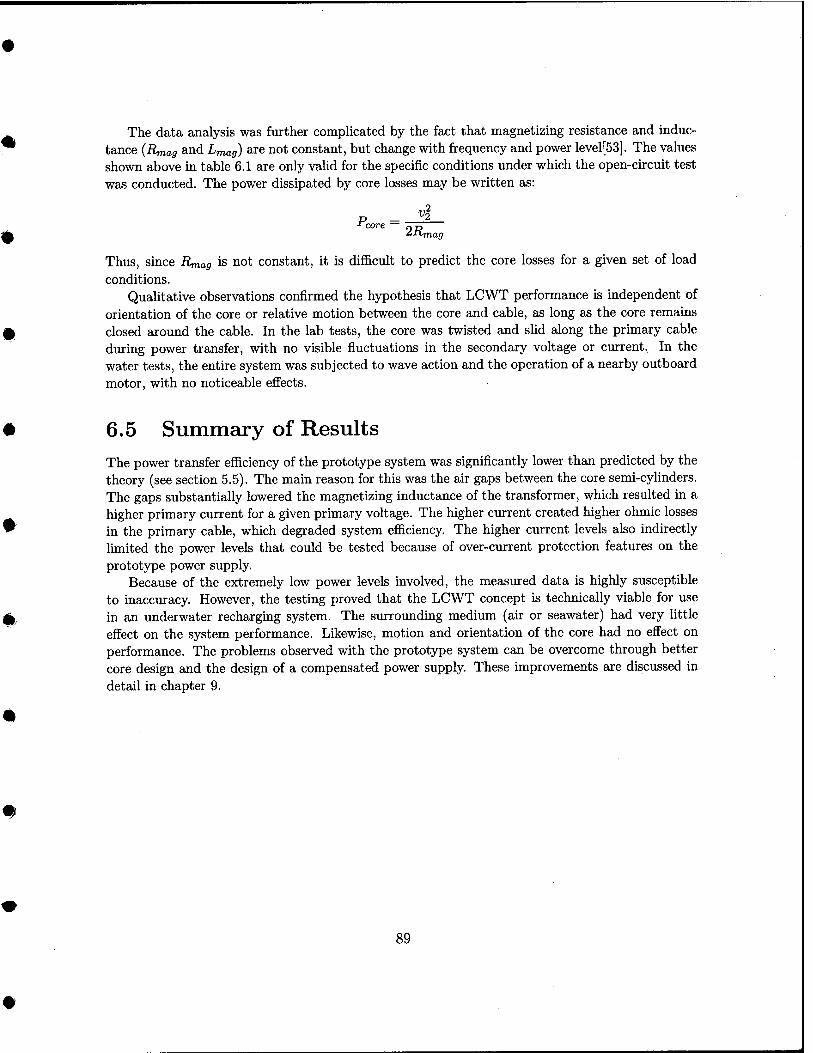
The data analysis was further comphcated by the fact that magnetizing resistance and induc- tance {Rmag and Lmag) are not constant, but change with frequency and power level[53]. The values shown above in table 6.1 are only vaUd for the specific conditions under which the open-circuit test was conducted. The power dissipated by core losses may be written as:
1)2
^ttftiag
Thus, since Rmag is not constant, it is difficult to predict the core losses for a given set of load conditions.
Qualitative observations confirmed the hypothesis that LCWT performance is independent of orientation of the core or relative motion between the core and cable, as long as the core remains closed around the cable. In the lab tests, the core was twisted and slid along the primary cable during power transfer, with no visible fiuctuations in the secondary voltage or current. In the water tests, the entire system was subjected to wave action and the operation of a nearby outboard motor, with no noticeable effects.
6.5 Summary of Results The power transfer efficiency of the prototype system was significantly lower than predicted by the theory (see section 5.5). The main reason for this was the air gaps between the core semi-cylinders. The gaps substantially lowered the magnetizing inductance of the transformer, which resulted in a higher primary current for a given primary voltage. The higher current created higher ohmic losses in the primary cable, which degraded system efficiency. The higher current levels also indirectly hmited the power levels that could be tested because of over-current protection features on the prototype power supply.
Because of the extremely low power levels involved, the measured data is highly susceptible to inaccviracy. However, the testing proved that the LCWT concept is technically viable for use in an underwater recharging system. The surrounding medium (air or seawater) had very little effect on the system performance. Likewise, motion and orientation of the core had no effect on performance. The problems observed with the prototype system can be overcome through better core design and the design of a compensated power supply. These improvements are discussed in detail in chapter 9.
89

This page intentionally blank
90
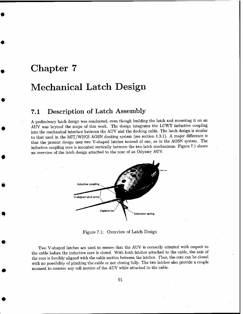
Chapter 7
Mechanical Latch Design
7.1 Description of Latch Assembly A preliminary latch design was conducted, even though building the latch and mounting it on an AUV was beyond the scope of this work. The design integrates the LCWT inductive coupling into the mechanical interface between the AUV and the docking cable. The latch design is similar to that used in the MIT/WHOI AOSN docking system (see section 1.3.1). A major difference is that the present design uses two V-shaped latches instead of one, as in the AOSN system. The inductive coupling core is mounted vertically between the two latch mechanisms. Figure 7.1 shows an overview of the latch design attached to the nose of an Odyssey AUV.
Inductive coupling
Extension spring
Figure 7.1: Overview of Latch Design
Two V-shaped latches are used to ensure that the AUV is correctly oriented with respect to the cable before the inductive core is closed. With both latches attached to the cable, the axis of the core is forcibly aUgned with the cable section between the latches. Thus, the core can be closed with no possibility of pinching the cable or not closing fully. The two latches also provide a couple moment to counter any roll motion of the AUV while attached to the cable.
91
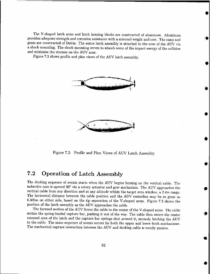
The V-shaped latch arms and latch housing blocks are constructed of aluminum. Aluminum provides adequate strength and corrosion resistance with a minimal weight and cost. The cams and gears are constructed of Delrin. The entire latch assembly is attached to the nose of the AUV via a shock mounting. The shock mounting serves to absorb some of the impact energy of the collision and minimize the stresses on the AUV nose.
Figure 7.2 shows profile and plan views of the AUV latch assembly.
Figure 7.2: Profile and Plan Views of AUV Latch Assembly
7.2 Operation of Latch Assembly
The docking sequence of events starts when the AUV begins homing on the vertical cable. The inductive core is opened 90° via a rotary actuator and gear mechanism. The AUV approaches the vertical cable from any direction and at any altitude within the target area window, a 2.4m range. The horizontal distance between the cable position and the AUV centerline may be as great as 0.305m on either side, based on the tip separation of the V-shaped arms. Figure 7.3 shows the position of the latch assembly as the AUV approaches the cable.
The forward motion of the AUV forces the cable to the center of the V-shaped arms. The cable strikes the spring-loaded capture bar, pushing it out of the way. The cable then enters the center recessed area of the latch and the capture bar springs shut around it, securely latching the AUV to the cable. The same sequence of events occurs for both the upper and lower latch mechanisms. The mechanical capture interaction between the AUV and docking cable is totally passive.
92
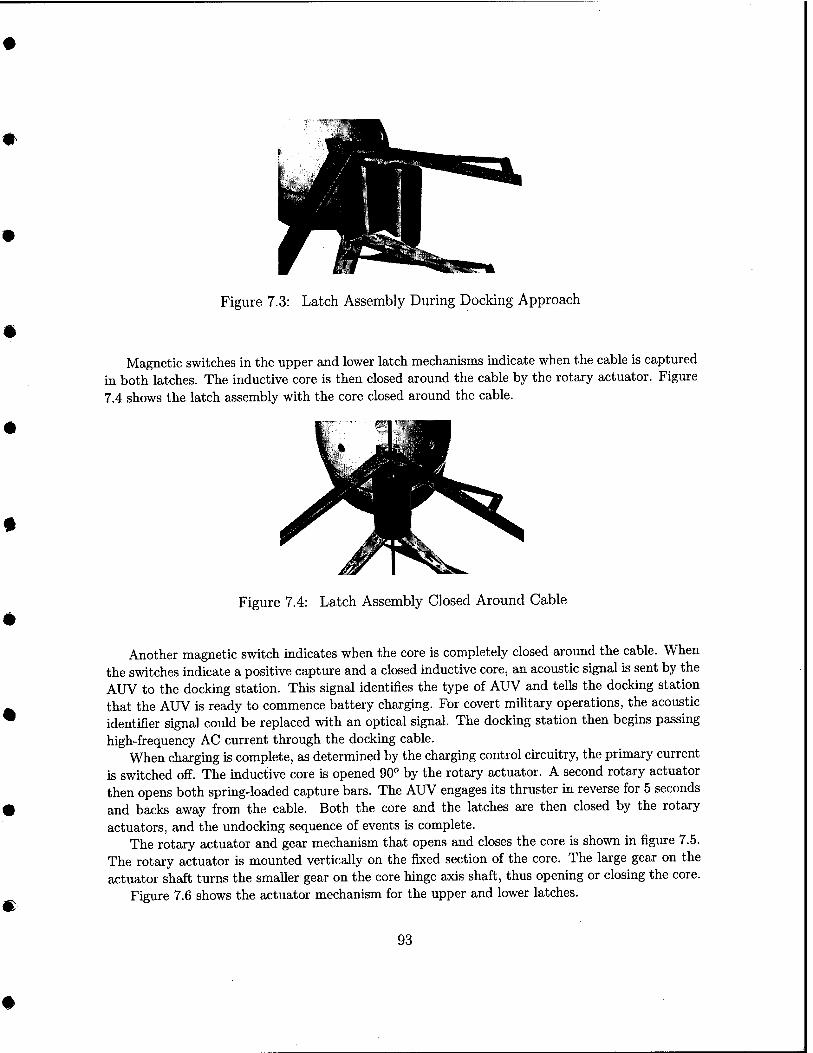
Figure 7.3: Latch Assembly During Docking Approach
Magnetic switches in the upper and lower latch mechanisms indicate when the cable is captured in both latches. The inductive core is then closed around the cable by the rotary actuator. Figure 7.4 shows the latch assembly with the core closed around the cable.
Figure 7.4: Latch Assembly Closed Around Cable
Another magnetic switch indicates when the core is completely closed around the cable. When the switches indicate a positive capture and a closed inductive core, an acoustic signal is sent by the AUV to the docking station. This signal identifies the type of AUV and tells the docking station that the AUV is ready to commence battery charging. For covert military operations, the acoustic identifier signal could be replaced with an optical signal. The docking station then begins passing high-frequency AC current through the docking cable.
When charging is complete, as determined by the charging control circuitry, the primary current is switched off. The inductive core is opened 90° by the rotary actuator. A second rotary actuator then opens both spring-loaded capture bars. The AUV engages its thruster in reverse for 5 seconds and backs away from the cable. Both the core and the latches are then closed by the rotary actuators, and the undocking sequence of events is complete.
The rotary actuator and gear mechanism that opens and closes the core is shown in figure 7.5. The rotary actuator is mounted vertically on the fixed section of the core. The large gear on the actuator shaft turns the smaller gear on the core hinge axis shaft, thus opening or closing the core.
Figure 7.6 shows the actuator mechanism for the upper and lower latches.
93
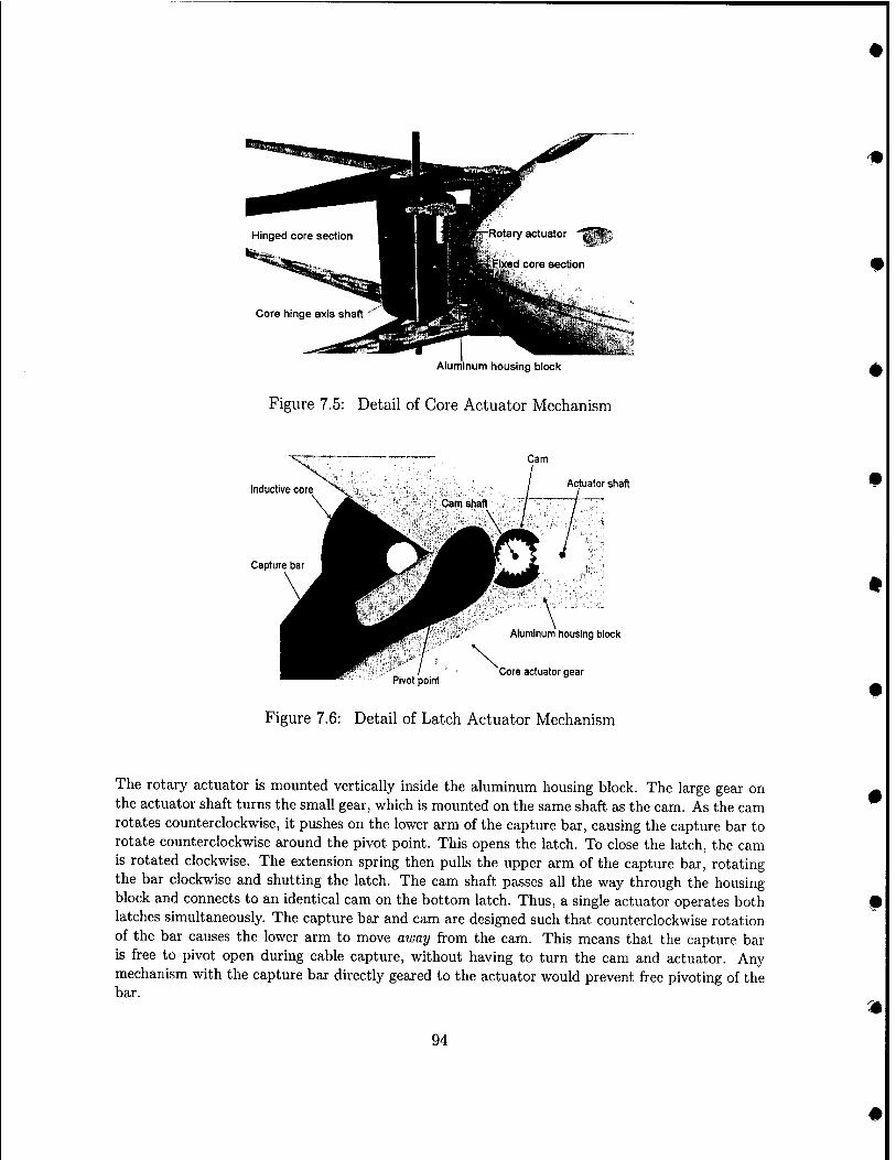
Aluminum housing block
Figure 7.5: Detail of Core Actuator Mechanism
Cam
Inductive core ^v
Capture bar
Actuator shaft
\ Aluminum housing block
Core actuator gear
Figure 7.6: Detail of Latch Actuator Mechanism
The rotary actuator is mounted vertically inside the aluminum housing block. The large gear on the actuator shaft turns the small gear, which is mounted on the same shaft as the cam. As the cam rotates counterclockwise, it pushes on the lower arm of the capture bar, causing the capture bar to rotate counterclockwise around the pivot point. This opens the latch. To close the latch, the cam is rotated clockwise. The extension spring then pulls the upper arm of the capture bar, rotating the bar clockwise and shutting the latch. The cam shaft passes all the way through the housing block and connects to an identical cam on the bottom latch. Thus, a single actuator operates both latches simultaneously. The capture bar and cam are designed such that counterclockwise rotation of the bar causes the lower arm to move away from the cam. This means that the capture bar is free to pivot open during cable captme, without having to turn the cam and actuator. Any mechanism with the capture bar directly geared to the actuator would prevent free pivoting of the bar.
94
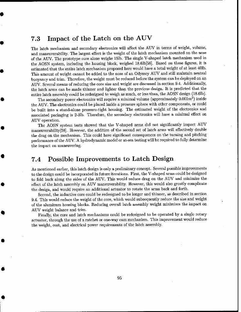
7.3 Impact of the Latch on the AUV The latch mechanism and secondary electronics will affect the AUV in terms of weight, volume, and maneuverability. The largest effect is the weight of the latch mechanism mounted on the nose of the AUV. The prototype core alone weighs 151b. The single V-shaped latch mechanism used in the AOSN system, including the housing block, weighed 18.61b[58]. Based on these figures, it is estimated that the entire latch mechanism proposed here would have a total weight of at least 401b. This amount of weight cannot be added to the nose of an Odyssey AUV and still maintain neutral buoyancy and trim. Therefore, the weight must be reduced before the system can be deployed on an AUV. Several means of reducing the core size and weight are discussed in section 9.4. Additionally, the latch arms can be made thinner and lighter than the previous design. It is predicted that the entire latch assembly could be redesigned to weigh as much, or less than, the AOSN design (18.61b).
The secondary power electronics will require a minimal volume (approximately O.OOlm^) inside the AUV. The electronics could be placed inside a pressure sphere with other components, or could be built into a stand-alone pressure-tight housing. The estimated weight of the electronics and associated packaging is 2-31b. Therefore, the secondary electronics will have a minimal effect on AUV operation.
The AOSN system tests showed that the V-shaped arms did not significantly impact AUV maneuver ability [58]. However, the addition of the second set of latch arms will effectively double the drag on the mechanism. This could have significant consequences on the turning and pitching performance of the AUV. A hydrodynamic model or at-sea testing will be required to fully determine the impact on maneuvering.
7.4 Possible Improvements to Latch Design As mentioned ear her, this latch design is only a prehminary concept. Several possible improvements to the design could be incorporated in future iterations. First, the V-shaped arms could be designed to fold back along the sides of the AUV. This would reduce drag on the AUV and minimize the effect of the latch assembly on AUV maneuverability. However, this would also greatly comphcate the design, and would require an additional actuator to rotate the arms back and forth.
Second, the inductive core could be redesigned to be longer and thinner, as described in section 9.4. This would reduce the weight of the core, which would subsequently reduce the size and weight of the aluminum housing blocks. Reducing overall latch assembly weight minimizes the impact on AUV weight balance and trim.
Finally, the core and latch mechanisms could be redesigned to be operated by a single rotary actuator, through the use of a ratchet or one-way cam mechanism. This improvement would reduce the weight, cost, and electrical power requirements of the latch assembly.
95

This page intentionally blank
96
#
Chapter 8
Economic Feasibility
The economic feasibility of the proposed AUV recharge system was evaluated using conventional discounted cash flow (DCF) analysis. The status quo methodology of operating AUVs from a support ship and recovering them to the ship for recharge after each sortie was compared to the methodology of deploying an underwater recharge system with the AUVs. The cost savings created by the latter operational strategy were computed for both military and commercial apphcation examples.
8.1 Military Application
8.1.1 Scenario and Assumptions The military AUV scenario considered was a hypothetical coastal surveillance mission. At least one REMUS AUV must be on station continuously for a 7 day period. Twenty such missions will be conducted per year. For security purposes, the support ship must remain 10 miles away from the target site. The ship is a Littoral Combat Ship (LCS), a next-generation small surface combatant equipped with AUV support systems. According to Congressional Budget OfSce projections, thfe LCS will have operating costs of $38,356 per day. For comparison, a destroyer (DDG-51) has typical operating costs of $71,233 per day[59]. The LCS is assumed to have the capability to launch or recover only one AUV at a time and to recharge as many AUVs as needed simultaneously. The REMUS AUV has a sortie endurance of approximately 20 hours at a speed of 3 knots, and operating costs of $180 per hoiu: (see section 2.1.4).
The status quo methodology requires the LCS to remain in position throughout the entire 7 day mission because the AUVs must transit back and forth from the LCS to the target site every sortie. The 10 mile transit takes 3.5 hours each direction. This leaves a maximum of 13 hours on station per sortie. It is estimated that the AUV turnaround time onboard the LCS will be about 3 hours. The batteries are removed from the AUV and replaced with fresh ones, allowing faster turnaround^ Thus, the total time the AUV is off station is 10 hours (7 hours transit+3 hours turnaround). The maximum on station time is 13 hours (20 hours endurance-7 hours transit). Since the maximum on station time is greater than the off station time, the mission can be accomplished by two alternating AUVs. To evenly distribute the on station time, each AUV remains on station 11 hours instead
^Typical recharge time for lithium polymer batteries is 6-8 hours.
97
of the possible maximum 13 . This allows a 30 minute overlap at the end of each exchange and ensures continuous AUV mission coverage.
The underwater recharge system methodology in this scenario uses a mobile tanker AUV (see section 2.1.3). The tanker AUV can transit undetected into the target site while the LCS remains some distance away, allowing covert AUV operations. The assumed tanker can support the entire 7 day mission without returning to the LCS. Thus, the LCS is free to leave the area and conduct other missions after deploying the tanker and REMUS AUVs, returning to retrieve them at the end of the mission. A conservative time of 2 ship-days per mission (1 day to deploy, 1 day to retrieve) was used in the calculations. Two REMUS AUVs are required for the mission, one on station while the other recharges from the tanker. A 10% time overlap is assumed for each AUV rotation, ensuring continuous mission coverage. The time spent attached to the tanker is not counted as AUV operating time, because all AUV systems are shut down. The acquisition and operating costs for the tanker AUV were estimated based on costs of similar systems. The tanker acquisition cost is paid as a lump sum at the start of the project. Additionally, the tanker was predicted to have a salvage value of 10% of original cost at the end of its 10 year service life.
Since both methodologies require 2 REMUS AUVs, the acquisition costs, service life, and salvage values for the AUVs were common to both methods and need not be included in the calculations. Additionally, the acquisition cost of the LCS is not included because it also is common to both methods. The ship operating costs include production of electricity; therefore no additional cost for the AUV recharge energy is explicitly included.
The DCF analysis was done in accordance with 0MB Circular A-94: Guidelines and Discount Rates for Benefit-Cost Analysis of Federal Programs[60]. All values were assumed to be constant- dollar (real) values. The calculations were done using a real 10 year discount rate of 2.1%[60]. All operating costs were taken as annual amounts paid at the end of the year. The two methodologies were compared over equal time periods so that both yielded equal benefits, with the exception of the tanker salvage value. Thus, the comparison was really a cost-effectiveness analysis. Only the discounted costs and the discounted salvage value needed to be calculated. This technique avoided having to quantify the benefits of either methodology.
Several of the variables used in the DCF calculations (missions per year, tanker service life, tanker acquisition cost, tanker operating costs, LCS operating costs, and discount rate) contained some associated uncertainty. The variables were assumed to follow normal distributions. The mean value of each variable was estimated based on historical data for similar systems. Additionally, the 5th percentile and 95th percentile values for each variable were estimated based on the level of uncertainty associated with the mean. The 5th and 95th percentiles define the range within which the actual value is expected to fall, with 90% confidence. The standard deviation (a) for each variable was then calculated. Equations are shown in Appendix E. The remaining two variables (REMUS operating costs and mission length) were either based on solid historical data or were specified to define the scenario, and were therefore not subject to uncertainty. The values used in the military scenario cost-effectiveness analysis are summarized in Table 8.1.
98
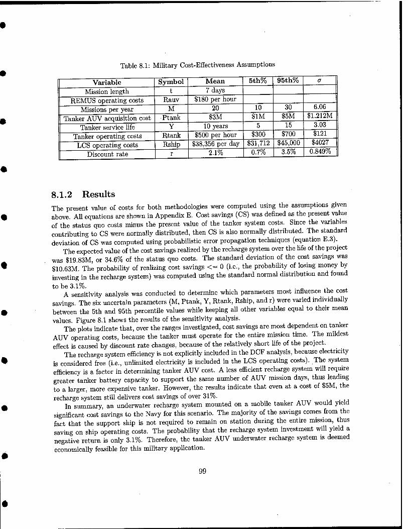
Table 8.1: Military Cost-Effectiveness Assumptions
Variable Symbol Mean 5th% 95th% a
Mission length t 7 days
REMUS operating costs Rauv $180 per hour
Missions per year M 20 10 30 6.06
Tanker AUV acquisition cost Ptank $3M $1M $5M $1.212M
Tanker service life Y 10 years 5 15 3.03
Tanker operating costs Rtank $500 per hour $300 $700 $121
LCS operating costs Rship $38,356 per day $31,712 $45,000 $4027
Discount rate r 2.1% 0.7% 3.5% 0.849%
8.1.2 Results The present value of costs for both methodologies were computed using the assumptions given above. All equations are shown in Appendix E. Cost savings (CS) was defined as the present value of the status quo costs minus the present value of the tanker system costs. Since the variables contributing to CS were normally distributed, then CS is also normally distributed. The standard deviation of CS was computed using probabilistic error propagation techniques (equation E.3).
The expected value of the cost savings reaUzed by the recharge system over the Hfe of the project was $19.83M, or 34.6% of the status quo costs. The standard deviation of the cost savings was $10 63M. The probability of realizing cost savings <= 0 (i.e., the probability of losing money by investing in the recharge system) was computed using the standard normal distribution and found
to be 3.1%. . „ ^. . A sensitivity analysis was conducted to determine which parameters most influence the cost
savings. The sbc uncertain parameters (M, Ptank, Y, Rtank, Rship, and r) were varied individually between the 5th and 95th percentile values while keeping all other variables equal to their mean values. Figure 8.1 shows the results of the sensitivity analysis.
The plots indicate that, over the ranges investigated, cost savings are most dependent on tanker AUV operating costs, because the tanker must operate for the entire mission time. The mildest effect is caused by discount rate changes, because of the relatively short Ufe of the project.
The recharge system efficiency is not explicitly included in the DCF analysis, because electricity is considered free (i.e., unlimited electricity is included in the LCS operating costs). The system efficiency is a factor in determining tanker AUV cost. A less efficient recharge system will require greater tanker battery capacity to support the same number of AUV mission days, thus leading to a larger, more expensive tanker. However, the results indicate that even at a cost of $5M, the recharge system still delivers cost savings of over 31%.
In summary, an underwater recharge system mounted on a mobile tanker AUV would yield significant cost savings to the Navy for this scenario. The majority of the savings comes from the fact that the support ship is not required to remain on station during the entire mission, thus saving on ship operating costs. The probability that the recharge system investment will yield a negative return is only 3.1%. Therefore, the tanker AUV underwater recharge system is deemed economically feasible for this military appUcation.
99
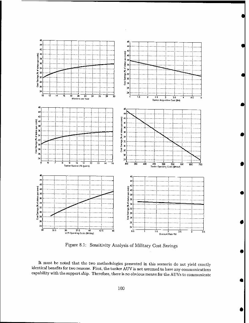
Missions pgr Year 2 2,5 3 3.5 4
Tanker Acquisition Cost (JM)
u : i i... —I 1 i— 1
42 : : j... .,.; J ■,..
o
= 38
j ; f- -j ■; \- -4
S36
»3.
"*'"'! 1 1 " 33rt £32 -;;>-'^1"-"f--- ■■■\ -i \- • --•: 1- ■ i -!••■■ ■■■< -i i— ■ ■■■i -
i 1 f- -i ■; \- ■-i - "26 ■ : r- ■■■i ■; ;■■ • --; -
24 1 1 \
-■■'v i--. 1 1 —]—.'.'] f" ■ -■! - <
8 9 10 11 12 Tanker Service Life (years)
<5D 500 550 600 Tanter Operating C:sts ($*ou^
35 37 5 40 LCS Operating Costs (Jkyday)
46
44
^42
S 40 o S-38 3 5 36
1 34 & &32
I 30 en -^
o
15 2 2.5 Discount Rale (%\
Figure 8.1: Sensitivity Analysis of Military Cost Savings
It must be noted that the two methodologies presented in this scenario do not yield exactly identical benefits for two reasons. First, the tanker AUV is not assumed to have any communications capability with the support ship. Therefore, there is no obvious means for the AUVs to communicate
100
time-critical data to the ship during the mission. In the status quo methodology, the data can be downloaded every time the AUV returns to the ship for recharging (i.e., every 11 hours instead of 7 days). Thus, the data retrieval benefit is not equal for both methodologies. The problem of communications could be solved several ways, one of which would be a communications buoy that is extended from the tanker AUV to the surface to allow RF communications. This method, however, compromises stealth. To make a truly equal comparison of the two methodologies, the costs associated with the tanker AUV should be increased by a penalty factor.
The second difference in benefits between the two methodologies is the ability to perform corrective maintenance during the mission. In the status quo methodology, small maintenance tasks may be performed while the AUV is onboard for recharging. In the tanker AUV methodology, this luxury does not exist. Thus, the reliability of the tanker AUV methodology is hkely to be lower. Therefore, the costs associated with the tanker AUV should again be increased by a penalty factor. However, despite these two penalty factors, the underwater recharge system is still expected to be cost effective.
8.2 Commercial Application
8.2.1 Scenario and Assumptions The commercial AUV scenario considered was a deep-water survey in the oil and gas industry. Cost effectiveness was computed firom the viewpoint of the oil company conducting the survey. The smvey AUV and support ship are leased by the oil company from an operator such as C&C Technologies. The survey AUV was a hypothetical vehicle similar in size and capabihty to the Hugin 3000, but equipped with rechargeable lithium polymer batteries rather than a semi-fuel cell power plant. The AUV was assumed to carry 20kWh of battery power, giving it a sortie endurance of 20 hours at a power consumption rate of 1 kW^.
The status quo methodology requires the support ship to shadow the AUV throughout the entire survey. The AUV is deployed from the ship, completes a sortie of 20 hours duration, then is recovered to the ship. Onboard, the AUV batteries are replaced with fresh ones and the cycle is repeated. The onboard turnaround time was estimated to be 4 hours, giving a total cycle time of 24 hours. The survey was assumed to take 6 days, or 6 cycles, based on similar surveys performed by the Hugin 3000. The day rate for the AUV and support ship was taken as $55K/day, based on Hugin 3000 data, yielding a total survey cost of $330K[37]. It was estimated that the oil company would conduct 10 such surveys per year.
The underwater recharge system methodology in this scenario used a moored docking station that is deployed fi-om the support ship at the same time as the AUV, then recovered with the AUV at the end of the survey. A moored dock was used rather than a tanker AUV because of the simpler design and lower cost. Additionally, the commercial survey scenario does not require covertness like the military scenario, thus negating the major advantage of the tanker AUV over a moored dock.
It was estimated that every 20 hour AUV sortie would be followed by an 8 hour recharge period at the docking station. Thus, an AUV cycle takes 28 hours compared to only 24 hours for the status quo methodology. Since the survey takes a total of 6 AUV cycles to complete, this results in a total
^The Hugin 3000 operates at a nominal power load of 900W[5].
101
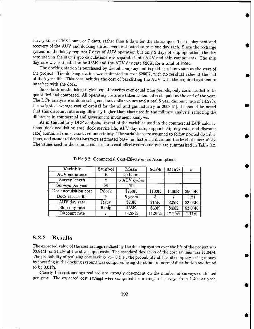
survey time of 168 hours, or 7 days, rather than 6 days for the status quo. The deployment and recovery of the AUV and docking station were estimated to take one day each. Since the recharge system methodology requires 7 days of AUV operation but only 2 days of ship operation, the day rate used in the status quo calculations was separated into AUV and ship components. The ship day rate was estimated to be $35K and the AUV day rate $20K, for a total of $55K.
The docking station is purchased by the oil company and is paid as a lump sum at the start of the project. The docking station was estimated to cost $250K, with no residual value at the end of its 5 year life. This cost includes the cost of backfitting the AUV with the required systems to interface with the dock.
Since both methodologies yield equal benefits over equal time periods, only costs needed to be quantified and compared. All operating costs are taken as annual costs paid at the end of the year. The DCF analysis was done using constant-dollar values and a real 5 year discount rate of 14.28%, the weighted average cost of capital for the oil and gas industry in 2003[61]. It should be noted that this discount rate is significantly higher than that used in the military analysis, reflecting the difference in commercial and government investment analyses.
As in the military DCF analysis, several of the variables used in the commercial DCF calcula- tions (dock acquisition cost, dock service hfe, AUV day rate, support ship day rate, and discount rate) contained some associated uncertainty. The variables were assumed to follow normal distribu- tions, and standard deviations were estimated based on historical data and the level of uncertainty. The values used in the commercial scenario cost-effectiveness analysis are summarized in Table 8.2.
Table 8.2: Commercial Cost-Effectiveness Assumptions
Variable Symbol Mean 5th% 95th% a AUV endurance E 20 hours Survey length t 6 AUV cycles
Surveys per year M 10 Dock acquisition cost Pdock $250K $100K $400K $90.9K
Dock service life Y 5 years 3 7 1.21 AUV day rate Rauv $20K $15K $25K $3.03K Ship day rate Rship $35K $30K $40K $3.03K Discount rate r 14.28% 11.36% 17.20% 1.77%
8.2.2 Results
The expected value of the cost savings realized by the docking system over the life of the project was $3.84M, or 34.1% of the status quo costs. The standard deviation of the cost savings was $1.04M. The probabiHty of realizing cost savings <= 0 (i.e., the probabihty of the oil company losing money by investing in the docking system) was computed using the standard normal distribution and found to be 0.01%.
Clearly the cost savings realized are strongly dependent on the number of surveys conducted per year. The expected cost savings were computed for a range of surveys from 1-40 per year.
102
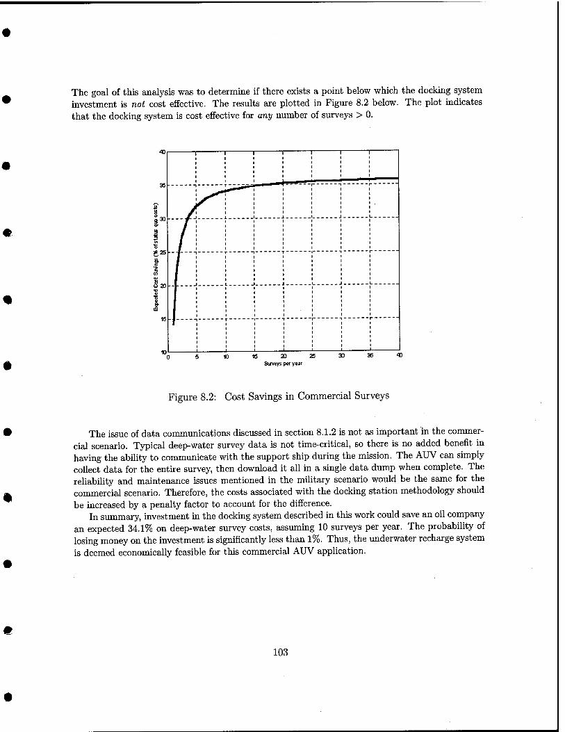
The goal of this analysis was to determine if there exists a point below which the docking system investment is not cost effective. The results are plotted in Figure 8.2 below. The plot indicates that the docking system is cost effective for any number of surveys > 0.
8 Q 30
!9 IS
•s » 25
CD
8
« ■s
1 1 1 1 1 1 \
1 I ^^ II —
Jfj 1 1 1 1 J 1
15 20 25
SuTveys per year
30 4)
Figure 8.2: Cost Savings in Commercial Surveys
The issue of data communications discussed in section 8.1.2 is not as important in the commer- cial scenario. Typical deep-water survey data is not time-critical, so there is no added benefit in having the abihty to communicate with the support ship during the mission. The AUV can simply collect data for the entire survey, then download it all in a single data dump when complete. The reliabihty and maintenance issues mentioned in the mihtary scenario would be the same for the commercial scenario. Therefore, the costs associated with the docking station methodology should be increased by a penalty factor to account for the difference.
In summary, investment in the docking system described in this work could save an oil company an expected 34.1% on deep-water survey costs, assuming 10 surveys per year. The probability of losing money on the investment is significantly less than 1%. Thus, the underwater recharge system is deemed economically feasible for this commercial AUV application.
103

This page intentionally blank
104
Chapter 9
Conclusions and Future Work
9.1 Demand for an AUV Recharge System The utility of present AUVs is limited by their on-board energy storage capability. Several alterna- tive AUV energy sources exist, such as rechargeable batteries, semi-fuel cells, fuel cells, and closed- cycle diesel engines. An analysis of the different energy source technologies and their prospects for the future was conducted. The results indicate that, in the near-term, rechargeable batter- ies will continue to be the power source of choice for most commercial and military AUVs. The other solutions were deemed to be too expensive or the technology too risky and unproven to see widespread proliferation in the industry. Thus, a demand exists for longer endmance rechargeable battery systems. Extensive research has already been done, and is ongoing, into the development of batteries with higher energy densities and longer cycle times. An alternative, which this work addressed, is the development of a system to recharge batteries in situ, without recovering the AUV to a support ship.
The United States Navy is a leading user and developer of AUVs in the world. The Navy has plans for a wide range of AUV systems and missions for the near future. Military AUV applications often require covertness or a large standoff distance between the support ship and the AUV operating area. An underwater recharging system will allow a network of AUVs to remain on station for extended periods without the presence of a support ship. An effective AUV recharging system is critical to the full realization of the Navy's net-centric warfare concept.
Commercial applications of AUVs are largely driven by the oil and gas industry. Commercial AUVs are mainly used for deepwater survey, where they are more efficient and yield better data than traditional towed systems. Work is also underway to develop AUVs or hybrid ROV-AUVs capable of subsea intervention. The major factor in the expense of operating AUVs is the dayrate of the support ship. An underwater recharging system with an industry-standard interface between AUV and dock is needed to reduce the dependence of AUVs on support ships. The system investigated in this work provides a technically and economically feasible solution.
105
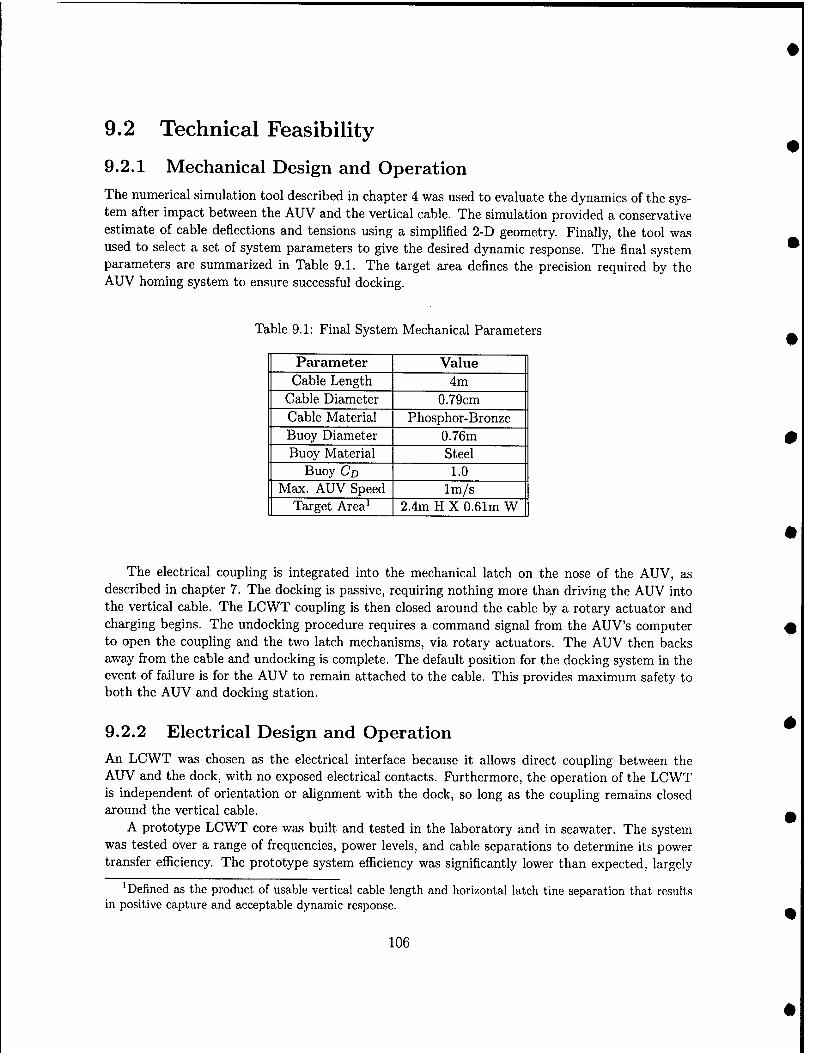
9.2 Technical Feasibility
9.2.1 Mechanical Design and Operation
The numerical simulation tool described in chapter 4 was used to evaluate the dynamics of the sys- tem after impact between the AUV and the vertical cable. The simulation provided a conservative estimate of cable deflections and tensions using a simplified 2-D geometry. Finally, the tool was used to select a set of system parameters to give the desired dynamic response. The final system parameters are summarized in Table 9.1. The target area defines the precision required by the AUV homing system to ensure successful docking.
Table 9.1: Final System Mechanical Parameters
Parameter Value Cable Length 4m
Cable Diameter 0.79cm Cable Material Phosphor-Bronze Buoy Diameter 0.76m Buoy Material Steel
Buoy CD 1.0 Max. AUV Speed Im/s
Target Area^ 2.4m H X 0.61m W
The electrical coupling is integrated into the mechanical latch on the nose of the AUV, as described in chapter 7. The docking is passive, requiring nothing more than driving the AUV into the vertical cable. The LCWT coupling is then closed around the cable by a rotary actuator and charging begins. The undocking procedure requires a command signal from the AUV's computer to open the coupling and the two latch mechanisms, via rotary actuators. The AUV then backs away from the cable and undocking is complete. The default position for the docking system in the event of failure is for the AUV to remain attached to the cable. This provides maximum safety to both the AUV and docking station.
9.2.2 Electrical Design and Operation An LCWT wEis chosen as the electrical interface because it allows direct coupling between the AUV and the dock, with no exposed electrical contacts. Furthermore, the operation of the LCWT is independent of orientation or alignment with the dock, so long as the coupling remains closed around the vertical cable.
A prototype LCWT core was built and tested in the laboratory and in seawater. The system was tested over a range of frequencies, power levels, and cable separations to determine its power transfer efficiency. The prototype system efficiency was significantly lower than expected, largely
'Defined as the product of usable vertical cable length and horizontal latch tine separation that results in positive capture and acceptable dynamic response.
106
due to the air gaps between the core semi-cyhnders created during assembly. The gaps lowered the magnetizing inductance of the core, which increased the primary current for a given primary voltage, therefore increasing the ohmic losses in the primary cable and decreasing efficiency. However, the testing demonstrated that the surrounding medium (air or seawater) has little effect on LCWT performance. The efficiency of the system will be improved through the actions described in section 9.4.
The simplified system design proposed in this work eliminates many of the problems experienced by previous docking efforts, such as binding of docking mechanisms and corrosion of electrical contacts. It can accomodate a wide range of AUV sizes and shapes, and could be easily backfitted to existing AUVs. The dynamic simulation and electrical experimentation demonstrate the technical feasibility of the design.
9.3 Economic Feasibility The cost-effectiveness of the proposed recharge system was analyzed for a specific military AUV appUcation. It was determined that the recharge system could save the Navy 34.6% on AUV operating costs, compared to operations without a recharge system. The majority of the savings comes from the fact that a support ship is not required to remain on station during the entire mission, thus reducing ship operating costs. The probability that the recharge system investment will yield a negative return is only 3.1%. Therefore, the underwater recharge system was deemed cost-effective for military applications.
The cost-effectiveness of the proposed system in a commercial deepwater survey scenario was also analyzed. The recharge system could save an oil company 34.1% on survey costs, mostly due to reductions in support ship costs. The probabiUty of a negative return on the investment is significantly less than 1%. Thus, the underwater recharge system was deemed cost-effective for commercial applications as well.
In addition to the monetary benefits described above, the AUV recharging system provides several quafitative benefits to both military and commercial users. Investment in the recharge system now also opens up future opportunities for expanded AUV use. These opportunities can be treated as real options, and will only make the system more economically attractive. The real option method is explained as future work in section 9.4.4.
9.4 Future Work
9.4.1 Improved LCWT Core Design The LCWT core design could be greatly improved over the prototype system. First, a better magnetic material could be chosen for the core. The Si-Fe used in the prototype was chosen based mainly on maximum fiux density and cost. In retrospect, amorphous metaUic glass (C-glass) can operate at higher frequencies, has lower core losses, and has a higher relative permeability than Si-Fe. The higher frequency allows a smaller core cross-section for a given secondary voltage (see equation 5.1), which will reduce core weight. Lower core losses will directly increase power transfer efficiency. The higher relative permeability will increase the magnetizing inductance of the core
107
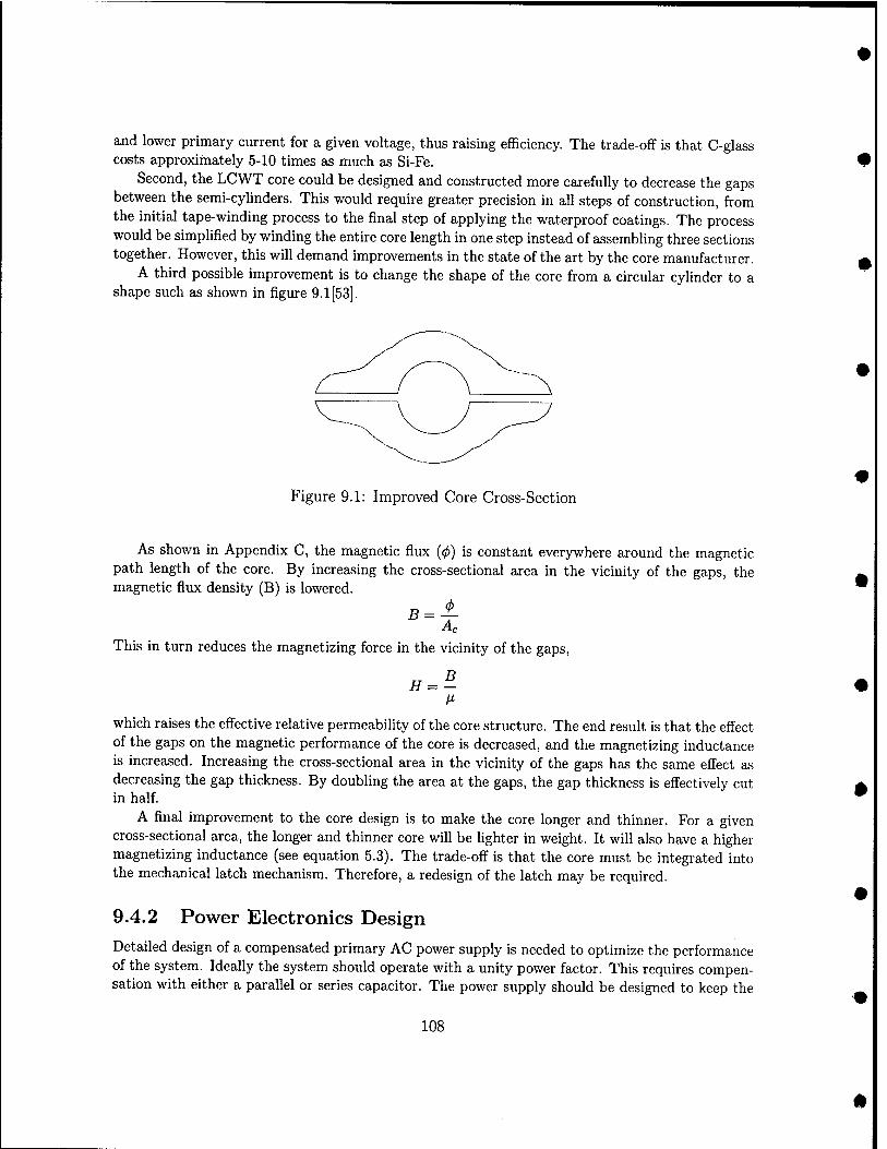
and lower primary current for a given voltage, thus raising efficiency. The trade-off is that C-glass costs approximately 5-10 times as much as Si-Fe.
Second, the LCWT core could be designed and constructed more carefully to decrease the gaps between the semi-cylinders. This would require greater precision in all steps of construction, from the initial tape-winding process to the final step of applying the waterproof coatings. The process would be simplified by winding the entire core length in one step instead of assembling three sections together. However, this will demand improvements in the state of the art by the core manufacturer.
A third possible improvement is to change the shape of the core from a circular cyhnder to a shape such as shown in figure 9.1 [53].
Figure 9.1: Improved Core Cross-Section
As shown in Appendix C, the magnetic flux ((/>) is constant everywhere around the magnetic path length of the core. By increasing the cross-sectional area in the vicinity of the gaps, the magnetic flux density (B) is lowered.
This in turn reduces the magnetizing force in the vicinity of the gaps,
fl = 5
which raises the effective relative permeability of the core structure. The end result is that the effect of the gaps on the magnetic performance of the core is decreased, and the magnetizing inductance is increased. Increasing the cross-sectional area in the vicinity of the gaps has the same effect as decreasing the gap thickness. By doubling the area at the gaps, the gap thickness is effectively cut in half.
A final improvement to the core design is to make the core longer and thinner. For a given cross-sectional area, the longer and thinner core will be lighter in weight. It will also have a higher magnetizing inductance (see equation 5.3). The trade-oflf is that the core must be integrated into the mechanical latch mechanism. Therefore, a redesign of the latch may be required.
9.4.2 Power Electronics Design
Detailed design of a compensated primary AC power supply is needed to optimize the performance of the system. Ideally the system should operate with a unity power factor. This requires compen- sation with either a parallel or series capacitor. The power supply should be designed to keep the
108
primary current as low as possible so as to limit ohmic losses in the cable. Additionally, the AC power supply must be designed to be driven by the DC batteries of the docking station or tanker
AUV. The secondary side power electronics on-board the AUV must also be designed. This subsystem
must rectify the AC signal from the LCWT, then convert the power to a form suitable to charge the AUV battery. The secondary electronics should be as small and hght as possible to minimize their impact on the AUV. This requirement overlaps with the need for an autonomous battery charging control system discussed below.
9.4.3 System Integration This work has demonstrated the mechanical and electrical feasibiUty of the proposed recharging system. The next step is to integrate the system into a docking station and AUV and test its performance in at-sea operations. This will involve at least four major actions:
1. Build the latch mechanism described in chapter 7 and mount it on an AUV.
2. Design and build a fixed docking station or tanker AUV to carry the vertical cable and AC
power supply.
3. Design and install a homing system to allow the AUV to reliably locate and dock with the
cable.
4. Design and install an autonomous battery charging control system.
9.4.4 Real Option Analysis In order to more accurately assess the economic feasibility of the recharge system, the conventional DCF analysis could be augmented with a real option analysis. The future opportunities that result from investment in the recharge system must be identified and quantified. For example Navy investment in the recharge system could allow extended AUV missions in areas that would otherwise be inaccessible, such as hostile harbors. If the Navy invests in the recharge system, it can decide in the future whether or not to conduct this type of mission. Without the recharge system, the choice does not exist. The value of this opportunity is not reflected in the DCF analysis The opportunity can be viewed as a choice that may or may not be exercised in the future, just like a call option. The real option approach requires mapping each future opportunity onto a call option. The option is then priced according to the Black-Scholes model. The total present value of the recharge system investment is then equal to the present value as calculated in chapter 8 plus the
value of all call options[62].
PV{total) = PV + Y^ {call option values)
The real option approach seeks to give credit for future opportunities created by investment in the recharge system. The value of the call options will always be positive; therefore, the real option analysis can only increase the present value of the investment and make it appear more economically viable. A real option analysis, combined with a conventional DCF analysis, will provide a more complete assessment of the proposed recharge system's economic feasibility.
109

This page intentionally blank
110

References
[1] A. Otsubo, K. Haga, and Y. Kowata, "Fast Reactor System for Underwater Activities," Proc. IEEE 2000 International Symposium on Underwater Technology, pp. 261-266, 2000.
[2] A. M. Bradley, M. D. Feezor, H. Singh, and F. Y. Sorrell, "Power Systems for Autonomous Underwater Vehicles," IEEE Journal of Oceanic Engineering, vol. 26 no. 4, pp. 526-538, Oct. 2001.
[3] T. Ura, H. Tabuchi, T. Obara, H. Maeda, and H. Yamato, "Development of Autonomous Vehicle with a Closed Cycle Diesel Engine," Proc. 18th Joint Meeting UJNR Marine Facilities Panel, pp. 179-188, Mar. 1993.
[4] G. T. Reader, I. J. Potter, E. J. Clavelle, and O. R. Fauvel, "Low Power StirUng Engine for Underwater Vehicle Applications," Proc. IEEE 1998 International Symposium on Underwater Technology, 1998.
[5] O. Hasvold and N. Storkersen, "Electrochemical Power Sources for Unmanned Underwater Vehicles Used in Deep Sea Survey Operations," Journal of Power Sources, vol. 96, pp. 252- 258, 2001.
[6] T. A. Dougherty, A. P. Karpinski, J. H. Stannard, W. HaUiop, and S. Warner, "Aluminum-Air: Status of Technology and Applications," Proc. 31st Intersociety Energy Conversion Engineer- ing Conference (lECEC 96), vol. 2, pp. 1176-1180, Aug. 1996.
[7] K. Vestgard and R. Hansen, "The Hugin 3000 Survey AUV Design and Field Results," [Online document], available
http://www.ivt.ntnu.no/imt/courses/tmr4240/exercises/HUGIN3000^urvey _AUV.pdf,
Oct. 2000, [cited Jan. 8, 2004].
[8] O. Hasvold, K. H. Johansen, O. MoUestad, S. Forseth, and N. Storkersen, "The Alkaline Aluminum/Hydrogen Peroxide Power Source in the Hugin II Unmanned Underwater Vehicle," Journal of Power Sources, vol. 80, pp. 254-260, 1999.
[9] G. E. Schubak and D. S. Scott, "A Techno-Economic Comparison of Power Systems for Au- tonomous Underwater Vehicles," IEEE Journal of Oceanic Engineering, vol. 20 no. 1, pp. 94-100, Jan. 1995.
[10] A. J. Appleby, "Fuel Cells and Hydrogen Fuel," International Journal of Hydrogen Energy, vol. 19 no. 2, pp. 175-180, 1994.
Ill
[11] G. Sattler, "Fuel Cells Going On-board," Journal of Power Sources, vol. 86, pp. 61-67, 2000.
[12] "World's First Fuel Cell Underwater Vehicle Successful," Sea-Japan, no. 301, Oct./Nov. 2003.
[13] G. MacKerron, "Financial Considerations of Exploiting Fuel Cell Technology," Journal of Power Sources, vol. 86, pp. 28-33, 2000.
[14] D. E. Frye, J. Kemp, W. Paul, and D. Peters, "Mooring Developments for Autonomous Ocean- Sampling Networks," IEEE Journal of Oceanic Engineering, vol. 26 no. 4, pp. 477-486, Oct. 2001.
[15] H. Singh, M. Bowen, F. Hover, P. LeBas, and D. Yoerger, "Intelligent Docking for an Au- tonomous Ocean Sampling Network," Oceans 97 MTS/IEEE Conference Proceedings. Halifax, Canada, 1997.
[16] R. Stokey, B. Allen, T. Austin, R. Goldsborough, N. Forrester, M. Purcell, and C. von Alt, "Enabling Technologies for REMUS Docking: An Integral Component of an Autonomous Ocean-Sampling Network," IEEE Journal of Oceanic Engineering, vol. 26 no. 4, pp. 487-497, Oct. 2001.
[17] R. Stokey, "Docking Background: Past, Present, and Future," presentation slides for AUV Fest 2001, Mar. 1999.
[18] T. Austin, "Concept of Operations," presentation slides for AUV Fest 2001, Mar. 1999.
[19] R. G. Di Cadilhac and A. Brighenti, " Docking Systems," in Technology and Applications of Autonomous Underwater Vehicles, G. Griffiths, Ed. New York, NY: Taylor and Francis Inc., 2003.
[20] S. Cowen, "Flying Plug: A Small UUV Designed for Submarine Data Connectivity," presented at Submarine Technology Symposium. Baltimore, MD, 1997.
[21] D. W. French, NUWC Code 8223 Head, "Two Tube Launch & Recovery Fbcture Brief: 30 July 2003," presentation shdes obtained from NUWC, Aug. 2003.
[22] "AUV Laboratory at MIT Sea Grant: Xanthos," [Online document], available http://auvlab.mit.edu/vehicles/vehiclespec2d.html, [cited Jan. 29, 2004].
[23] The Navy Unmanned Undersea Vehicle (UUV) Master Plan, prepared by a committee of participants under funding from PEO (USW) PMS403, Apr. 20, 2000.
[24] P. Higgins, NUWC Code 822 Division Head, "Autonomous Undersea Vehicles Division," pre- sented to Captain John C. Mickey, Apr. 2003.
[25] B. Fletcher, "The U.S. Navy's Master Plan: A Vision for UUV Development," Underwater Magazine, Jul./Aug. 2001.
[26] "REMUS Autonomous Underwater Vehicle," [Onhne document], available http://www.hydroidinc.com/brochure-web.pdf, [cited Jan. 10, 2004].
[27] L. P. Kasper, PMS NSW, "MK 14 MOD 0 Semi-Autonomous Hydrographic Reconnaissance Vehicle (SAHRV) System," presentation slides obtained from PMS NSW, Aug. 2003.
112
[28] B. Woodland, F. Brimberg, R. Sheriff, and J. Flanagan, "UUVs and Mine Warfare Systems," Sea Technology, pp. 63-69, Nov. 1997.
[29] R. L. Wernli, "Trends in UUV Development," Sea Technology, pp. 17-23, Dec. 1997.
[30] B. Bawek, "Conceptual 21-Inch Diameter MRUUV," presentation slides obtained from NUWC,
Jun. 2002.
[31] D. W. French, NUWC Code 8223 Head, "NUWCs Unmanned Undersea Vehicle (UUV) Test- beds," presentation slides obtained from NUWC, Aug. 2003.
[32] National Research Council, Network-Centric Naval Forces: A Transition Strategy for Enhanc- ing Operational Capabilities. Washington, DC: National Academy Press, 2000.
[33] B. Fletcher, "Autonomous Vehicles and the Net-Centric Battlespace," presented at Interna- tional UUV Symposium. Newport, RI, Apr. 2000.
[341 "Surface and Shallow Water Mine Counter measures: RDT&E Budget Item Justification," [On- line document], available http://www.dtic.mil/descriptivesum/Y2003/NAVY/0603502N.pdf,
Feb. 2002, [cited Jan. 20, 2004].
[351 "FY2003 Defense Budget," [Online document], available http://www.defenselink.mil/news/Feb2002/020201-D-6570C-001.pdf, Feb. 2002, [cited
Jan. 20, 2004].
[36] R. L. Wernh, "AUVs: The Maturity of the Technology," Oceans 99 MTS/IEEE Conference
Proceedings, 1999.
[37] R. L. Wernh, "AUV Commercialization: Who's Leading the Pack?," Oceans 2000 MTS/IEEE Conference Proceedings. Providence, RI, 2000.
[38] P. J. Ryan, "Mine Countermeasures a Success," The Naval Institute Proceedings, May 2003.
[39] C. von Alt, "REMUS 100 Transportable Mine Countermeasure Package," Oceans 2003 MTS/IEEE Conference Proceedings, 2003.
[40] "Side by Side Comparison: RMS vs. Submarine Baseline LMRS," presentation shde obtained
from NUWC, Oct. 2002.
[41] J. Westwood, "Future Prospects for AUVs," presentation to the Maridan 'PING' symposium.
Copenhagen, Sep. 1999.
[42] T S Chance "AUV Surveys: Extending Our Reach 24,000 Kilometers Later," [Onhne docu- ment], available http://www.cctechnol.com/papers/UUST03C&C.pdf, [cited Jan. 20, 2004].
[43] D. Bingham, T. Drake, A. Hill, and R. Lott, "The Apphcation of Autonomous Underwa- ter Vehicle (AUV) Technology in the Oil Industry - Vision and Experiences," [Online doc- ument] , available http://www.ddl.org/figtree/pub/fig-2002/Ts4-4/TS4.4_bingham_etal.pdf,
[cited Jan. 20, 2004].
[44] F. S. Hover, "Selection of Physical Parameters for the Odyssey II Vehicle," prepared for MIT SeaGrant Program, Jul. 1995.
113
[45] M. F. Spotts and T. E. Shoup, Design of Machine Elements. Upper Saddle River, NJ: Prentice Hall, 1998.
[46] J. W. Brewer, Engineering Analysis in Applied Mechanics. New York, NY: Taylor and Francis Inc., 2002.
[47] M. R. Lindeburg, Engineer-in-Training Reference Manual, 8th ed. Belmont, CA: Professional Publications Inc., 1992.
[48] S. F. Hoerner, Fluid-Dynamic Lift. Bakersfield, CA: Hoerner Fluid Dynamics, 1985.
[49] H. Singh, S. Lerner, K. Von Der Heyt, and B. Moran, "An Intelligent Dock for an Autonomous Ocean Sampling Network," Oceans 98 MTS/IEEE Conference Proceedings. Nice, France, 1998.
[50] "Ocean Innovations: Steel Subsurface Flotation," [Online document], available http://www.o- vations.com/steeLbuoys.html, [cited Jan. 20, 2004].
[51] S. F. Hoerner, Fluid-Dynamic Drag. Bakersfield, CA: Hoerner Fluid Dynamics, 1992.
[52] K. W. Klontz, D. M. Divan, D. W. Novotny, and R. D. Lorenz, "Contactless Power Delivery System for Mining Applications," IEEE Transactions on Industry Apphcations, vol. 31 no. 1, pp. 27-35, Jan./Feb. 1995.
[53] B. J. Heeres, D. W. Novotny, D. M. Divan, and R. D. Lorenz, "Contactless Underwater Power Delivery," 25th Annual IEEE Power Electronics Specialists Conference, PESO '94 Record, vol. 1, pp. 418-423, Jun. 1994.
[54] "Tape Wound Cores: Design Manual TWC 600," Magnetics Corporation, [Online document], available http://www.mag-inc.com/pdf/TWC-600.pdf, [cited Jan. 10, 2004].
[55] O. H. Stielau and G. A. Covic, "Design of Loosely Coupled Inductive Power Transfer Systems," IEEE International Conference on Power System Technology Proceedings, vol. 1, pp. 85-90, Dec. 2000.
[56] J. M. Barnard, J. A. Ferreira, and J. D. van Wyk, "Sliding Transformers for Linear Contactless Power Delivery," IEEE Transactions on Industrial Electronics, vol. 44 no. 6, pp. 774-779, Dec. 1997.
[57] G. R. Slemon, Magnetoelectric Devices: Transducers, Transformers, and Machines. New York, NY: John Wiley and Sons Inc., 1966.
[58] M. F. Bowen, "A Passive Capture Latch for ODYSSEY-Class AUVs," Woods Hole Oceano- graphic Institution Technical Report, WHOI-98-12, Jun. 1998.
[59] "Transforming the Navy's Surface Combatant Force: A CBO Study," Con- gressional Budget Office, Washington, DC. [Online document], available ftp://ftp.cbo.gov/41xx/doc4130/Report.pdf, March 2003, [cited Feb. 16, 2004].
[60] 0MB Circular A-94: Guidelines and Discount Rates for Benefit-Cost Analysis of Federal Programs, U.S. Government Office of Management and Budget, [Online document], available http://www.whitehouse.gov/omb/circulars/a094/a094.pdf, [cited Feb. 16, 2004].
114

[61] C. K. Strayhorn, "Determination of 2003 Discount Rate Range for Petroleum and Hard Mineral Properties," Texas Comptroller of Public Accounts, [Online document], available http://www.window.state.tx.us/taxinfo/proptax/drs03, Jul. 2003, [cited Feb. 16, 2004].
[62] T. A. Luehrman, "Investment Opportunities as Real Options: Getting Started on the Num- bers," Harvard Business Review, vol. 76 no. 4, pp. 51-61, Jul./Aug. 1998.
115

This page intentionally blank
116

Appendix A
Matlab Dynamic Simulation Codes
A.l Symbolic Formulation of Lagrange's Equations
'/.deriv. m
•/.Symbolically calculates partial derivatives of energy terms
'/.and formulates Lagrange's Equations
syms phil phi2 dell del2 phild plii2d delld del2d vpar vperp V LI L2 Cbuoy Cauv syms Ccable m M Ibuoy lauv Dphil Dphi2 Ddell Ddel2 T kl k2 cl c2
vperp=(Ll+dell)*phild+(L2+del2)*phi2d*cos(phil-phi2)-del2d*sin(phil-phi2);
vpar=(L2+del2)*phi2d*sin(phil-phi2)+delld+del2d*cos(phil-phi2);
V=(vperp'2+vpar"2)".5;'/.Total buoy velocity
•/.Virtual work Wbuoy=-Cbuoy*V*(((Ll+dell)*phil+(L2+del2)*plii2*cos(phil-phi2) -del2*sin(phil-phi2))*((Ll+dell)*phild+(L2+del2)*plii2d*cos(phil-phi2) -del2d*sin(phil-phi2))+((L2+del2)*phi2*sin(phil-phi2) +dell+del2*cos(phil-phi2))*((L2+del2)*phi2d*sin(phil-plii2)
+delld+del2d*cos(phil-phi2)));
Wauv=-Cauv*(Ll+dell)~3*phil*phild~2;
WL1=-Ccable*(Ll+dell)-4/4*phil*pliild-2;
WL2=-Ccable*(pMld-2*(Ll+dell)"3*(L2+del2)*phil*cos(phil-phi2)"3 +(Ll+dell)"2*(L2+del2)"2*phil*phild*phi2d*cos(phil-phi2)"2 + (L2+del2) "2/2* (Ll+dell) -2*p]ii2*pMld"2*cos(phil-phi2) ~1 +2/3* (Ll+dell) * (L2+del2) '•3*phi2*phild*phi2d*cos (phil-pM2) + (Ll+dell)/3*(L2+del2)-3*phil*phi2d-2*cos(phil-plii2) + (L2+del2)-4/4*plii2*pM2d-2);
117

W=Wbuoy+Wauv+WLl+WL2;
dWdphil=diff(W,phil) dWdphi2=diff(W,phi2) dWddell=diff(W,dell) dWddel2=diff(W,del2)
'/.Kinetic energy
Ktauv=.5*m*((Ll+dell)-2*phild-2+delld"2);
Krauv=.5*Iauv*phild"2;
Ktbuoy=.5*M*((Ll+dell)"2*phild*2+(L2+del2)*2*phi2d*2+delld"2+del2d~2
+2*delld*del2d*cos(phil-phi2)+2*(Ll+dell)*(L2+del2)*phild*phi2d*cos(phil-phi2) -2*(Ll+dell)*phild*del2d*sin(phil-phi2)+2*(L2+del2)*phi2d*delld*sin(phil-phi2));
Krbuoy=.5*Ibuoy*phi2d"2;
K=Kt auv+Krauv+Ktbuoy+Krbuoy;
dKdphil=diff(K,phil) dKdpM2=diff(K,phi2) dKddell=diff(K,dell) dKddel2=diff(K,del2) dKdphild=diff(K,phild) dKdphi2d=diff(K,phi2d) dKddelld=diff(K,delld) dKddel2d=diff(K,del2d)
•/.Time derivatives, using chain rule
dtdphild=diff(dKdphild,phil)*phild+diff(dKdphild,phi2)*phi2d
+diff(dKdphild,dell)*delld+diff(dKdphild,del2)*del2d+diff(dKdphild,phild)*Dphil +diff(dKdphild,phi2d)*Dphi2+diff(dKdphild,delld)*Ddell+diff(dKdphild,del2d)*Ddel2;
dtdphi2d=diff(dKdphi2d,phil)*phild+diff(dKdphi2d,phi2)*phi2d
+diff(dKdphi2d,dell)*delld+diff(dKdphi2d,del2)*del2d+diff(dKdphi2d,phild)*Dphil +diff(dKdphi2d,phi2d)*Dphi2+diff(dKdphi2d,delld)*Ddel1+diff(dKdphi2d,del2d)*Ddel2;
dtddelld=diff(dKddelld,phil)*phild+diff(dKddelld,phi2)*phi2d
+diff(dKddelld,dell)*delld+diff(dKddelld,del2)*del2d+diff(dKddelld,phild)*Dphil +diff(dKddelld,phi2d)*Dphi2+diff(dKddelld,delld)*Ddell+diff(dKddelld,del2d)*Ddel2;
dtddel2d=diff(dKddel2d,phil)*phild+diff(dKddel2d,phi2)*phi2d
+diff(dKddel2d,dell)*delld+diff(dKddel2d,del2)*del2d+diff(dKddel2d,phild)*Dphil
118
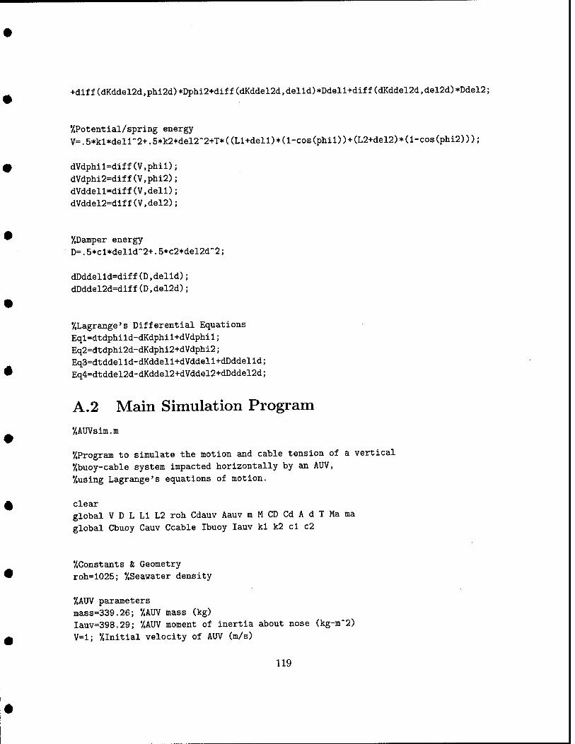
+diff(dKddel2d,phi2d)*Dphi2+diff(dKddel2d,delld)*Ddell+diff(dKddel2d,del2d)*Ddel2;
"/.Potential/spring energy V=.5*kl*dell"2+.5*k2*del2~2+T*((Ll+dell)*(1-cos(phil))+(L2+del2)*(1-cos(phi2)));
dVdphil=diff(V,phil) dVdphi2=diff(V.phi2)
dVddell=diff(V,dell) dVddel2=diff(V,del2)
'/.Damper energy D=.5*cl*delld~2+.5*c2*del2d'2;
dDddelld=diff(D,delld); dDddel2d=diff(D,del2d);
'/.Lagrange's Differential Equations Eql=dtdphild-dKdphil+dVdphil; Eq2=dtdphi2d-dKdphi2+dVdphi2; Eq3=dtddelld-dKddell+dVddell+dDddelld; Eq4=dtddel2d-dKddel2+dVddel2+dDddel2d;
A.2 Main Simulation Program
y,AUVsim.m
•/.Program to simulate the motion and cable tension of a vertical •/.buoy-cable system impacted horizontally by an AUV, •/.using Lagrange's equations of motion.
clear global V D L LI L2 roh Cdauv Aauv m M CD Cd A d T Ma ma
global Cbuoy Cauv Ccable Ibuoy lauv kl k2 cl c2
•/.Constants & Geometry roh=1025; '/.Seawater density
•/.AUV parameters mass=339.26; •/.AUV mass (kg) Iauv=398.29; •/.AUV moment of inertia about nose (kg-m"2) V=l; •/.Initial velocity of AUV (m/s)
119

Aauv=.252; '/.Frontal area of AUV Cdside=1.62;'/.Body Cross-flow drag coefficient (Hover) Aside=1.24;%Side plan area Ld=.98; '/.Distance from center of side drag to nose (m) cb=.98;'/.Distance from C.B. to nose (m)
ma=.l*mass; '/.Axial added mass of AUV m=mass+ma;
'/.Cable peirameters L=4; '/.Total cable length (m) Ll=1.5; '/.Height of impact (m) L2=L-L1; d=.00794; '/.Cable diameter (m) (5/16")
douter=.0119; '/.Outer dieuneter of coated cable (used for drag calcs) E=lell; '/.Young's Modulus of cable raw material (N/m*2)
Eeff=.43*E; '/.Effective Young's Modulus of wire rope Acable=.404*d"2; '/.Effective cable cross-section area Break=3680/.22448; '/.Breaking strength (N) FS=4; '/.Factor of safety for cable
'/.Buoy parameters Mass=55; '/.Buoy mass (kg) D=.76; '/.Buoy diameter (m)
Ibuoy=2/5*Mass*(D/2)'"2; '/.Buoy moment of inertia (kg-m'2) A=pi/4*D*2; '/.Projected area of buoy W=Mass*9.81; '/.Weight of buoy
B=4/3*pi*(D/2)"3*roh*9.81; '/.Buoyant force on buoy Ma=B/2/9.81; '/.Added mass of buoy M=Mass+Ma; T=1600; '/.Net upward force on buoy (B-Wbuoy-Wcable)
'/.Drag parameters Cd=1.2; '/.Drag coefficient for cable CD=1; '/.Drag coefficient for buoy Cdauv=0.07; '/.Frontal drag coefficient for AUV (Hover) Cbuoy=.5*roh*CD*A; Cauv=.5*roh*Cdauv*Aauv; Ccable=roh*Cd*douter; '/.(2 cables)
'/.Spring/Damping constants kl=Eef f *Acable/Ll; '/,N/m k2=Eef f *Acable/L2; '/.N/m freql=(kl/(m+M))-.5;'/.Natural freq of LI freq2=(k2/(m+M))".5;'/.Natural freq of L2
120
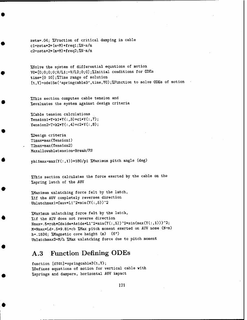
2eta=.04; '/.Fraction of critical damping in cable
cl=zeta*2* (m+M) *f reql; '/.N-s/m c2=zeta*2* (m+M) *f req2; '/.N-s/m
'/.Solve the system of differential equations of motion Y0=[0;0;0;0;V/L1;-V/L2;0;0] ;'/.Initial conditions for ODEs
time=[0 10];'/,Time range of solution [t,Y]=odel5s('springcable3',time,YO);'/.Function to solve ODEs of motion
'/.This section computes cable tension and '/.evaluates the system against design criteria
'/.Cable tension calculations Tensionl=T+kl*Y(:,3)+cl*Y(:,7); Tension2=T+k2*Y(:,4)+c2*Y(:,8);
'/.Design criteria Tlmax=max(Tensionl) T2max=max(Tension2) Maxallowabletension=Break/FS
philmax=max(Y(: ,l))*180/pi '/.Maximum pitch angle (deg)
•/.This section calculates the force exerted by the cable on the
'/.spring latch of the AUV
•/.Maximum unlatching force felt by the latch, '/.if the AUV Completely reverses direction Unlatchmaxl=Cauv*Ll"2*min(Y(:,5))"2
'/.Maximum unlatching force felt by the latch, '/.if the AUV does not reverse direction Nmax=.5*roh*Cdside*Aside*Ll"2*min(Y(:,5))"2*sin(max(Y(:,1)))"2;
M=Nmax*Ld+.5*9.81*cb '/.Max pitch moment exerted on AUV nose (N-m) h=.i524; •/.Magnetic core height (m) (6") Unlatchmax2=M/h •/.Max unlatching force due to pitch moment
A.3 Function Defining ODEs function [dYdt]=springcable3(t,Y); '/.Defines equations of motion for vertical cable with •/.springs and dampers, horizontal AUV impact
121
•/.including drag on AUV and added masses
global roh Cdauv Aauv m CD Cd M A d T Ma ma
global Cbuoy Cauv Ccable Ibuoy lauv kl k2 L LI L2 cl c2
•/.State variables, Y(t) phil=Y(l); phi2=Y(2) dell=Y(3) del2=Y(4) phild=Y(5)
phi2d=Y(6) delld=Y(7)
del2d=Y(8)
'/.Generalized non-conservative forces acting on system
•/.AUV Drag Fla=-Cauv*(Ll+dell)"3*phild*abs(phild); F2a=0; F3a=0 F4a=0
•/.Buoy Drag
xdot=(Ll+dell)*phild*cos(phil)+delld*sin(phil)+(L2+del2)*phi2d*cos(phi2) +del2d*sin(phi2);
ydot=-(Ll+dell)*phild*sin(phil)+delld*cos(phil)-(L2+del2)*phl2d*sin(phi2) +del2d*cos(phi2);
v=(xdot~2+ydot"2)~.5; Fx=-Cbuoy*v*xdot; Fy=-Cbuoy*v*ydot; Flb=Fx*(Ll+dell)*cos(phil)-Fy*(Ll+dell)*sin(phil); F2b=Fx*(L2+del2)*cos(phi2)-Fy*(L2+del2)*sin(phi2); F3b=Fx*sin(phil)+Fy*cos(phil); F4b=Fx*sin(phi2)+Fy*cos(phi2);
•/.Lower cable drag Flc=-l/4*Ccable*phild*abs(phild)*(Ll+dell)"4; F2c=0;
122

F3c=0; F4c=0;
•/.Upper cable drag F=-Ccable*((phild*abs(phild)*(Ll+dell)"2*cos(phil-phi2)-2+delld*abs(delld) *sin(phil-phi2)~2+2*pliild*(Ll+dell)*delld*cos(pMl-phi2)*sin(phil-pM2)) *(L2+del2)+l/3*phi2d*abs(phi2d)*(L2+del2)-3+(2*phild*(Ll+dell)*phi2d *cos(phil-phi2)+2*delld*phi2d*sin(phil-phi2))/2*(L2+del2)"2);
Fld=F*cos(pM2)*(Ll+dell)*cos(phil)+F*sin(p]ii2)*(Ll+dell)*sin(pMl);
F2d=3/4*F*(L2+del2); F3d=Fi'COs(pM2)*sin(phil)-F*sin(phi2)*cos(pMl);
F4d=0;
•/.Svim of all generalized forces Fl=Fla+Flb+Flc+Fld; F2=F2a+F2b+F2c+F2d; F3=F3a+F3b+F3c+F3d; F4=F4a+F4b+F4c+F4d;
•/.Matrix differential equations: N*Y'=S(t,Y)
•/oCoeffiecient matrix
Nl=eye(4); N2=zeros(4); N3=zeros(4); N4=[(m*Ll-2+2*m*Ll*dell+in*dell-2+Iauv+M*Ll-2+2*M*Ll*dell+M*dell-2) (M*cos(phil-phi2)*dell*del2+M*cos(p]iil-plii2)*Ll*L2+M*cos(phil-plii2)*Ll*del2
+M*cos(phil-phi2)*dell*L2) 0 (-M*sin(ph.il-phi2)*dell-M*sin(pMl-phl2)*Ll); (M*cos(pMl-phi2)*Ll*L2+M*cos(phil-plii2)*Ll*del2+M*cos(pliil-phi2)*dell*L2
+M*cos(phil-phi2)*dell*del2) (M*L2-2+2*M*L2*del2+M*del2-2+Ibuoy)
(M*sin(phil-plii2)*L2+M*sin(phil-plii2)*del2) 0; 0 (M*sin(phil-phi2)*L2+M*sin(pliil-phi2)*del2) (m+M) M*cos(p]ail-phi2); (-M*sin(phil-phi2)*Ll-M*sin(pMl-plii2)*dell) 0 M*cos(phil-phi2) M] ;
N=[N1 N2;N3 N4];
Sl=phild; S2=pM2d; S3=delld; S4=del2d;
123

S5=-(T*sin(phil)*dell+T*sin(phil)*Ll+2*delld*m*phild*Ll+2*delld*M*phild*dell +M*phi2d-2*sin(phil-phi2)*dell*del2+2*M*phi2d*del2d*cos(phil-phi2)*Ll +M*phi2d"2*sin(phil-phi2)*Ll*del2+M*phi2d''2*sin(phil-phi2)*dell*L2
+2*delld*in*phild*dell+2*delld*M*phild*Ll+2*M*phi2d*del2d*cos(phil-phi2)*dell +M*phi2d"2*sin(phil-phi2)*Ll*L2)+Fl;
S6=-(2*M*del2d*phi2d*L2+2*M*del2d*phi2d*del2-M*phild"2*sin(phil-phi2)*dell*L2 -M*phild"2*sin(phil-phi2)*dell*del2+2*M*phild*delld*cos(phil-phi2)*L2
-M*phild"2*sin(phil-phi2)*Ll*L2-M*phild"2*sin(phil-phi2)*Ll*del2+T*sin(phi2)*L2 +T*sin(phi2)♦del2+2*M*phild*delld*cos(phil-phi2)♦del2)+F2;
S7=-(2*M*phi2d*siii(phil-phi2)*del2d-M*phi2d"2*cos(phil-phi2)*L2
-M*phi2d"2*cos(phil-phi2)*del2-m*phild"2*Ll-m*phild"2*dell-M*phild"2*Ll -M*phild"2*dell+kl*dell+T-T*cos(phil)+cl*delld)+F3;
S8=-(-2*M*phild*sin(phil-phi2)*delld-M*phild-2*cos(phil-phi2)*Ll
-M*phild-2*cos(phil-phi2)*dell-M*phi2d-2*L2-M*phi2d-2*del2-T*cos(phi2) +c2*del2d+k2*del2+T)+F4;
dYdt=N\[Sl;S2;S3;S4;S5;S6;S7;S8];
124
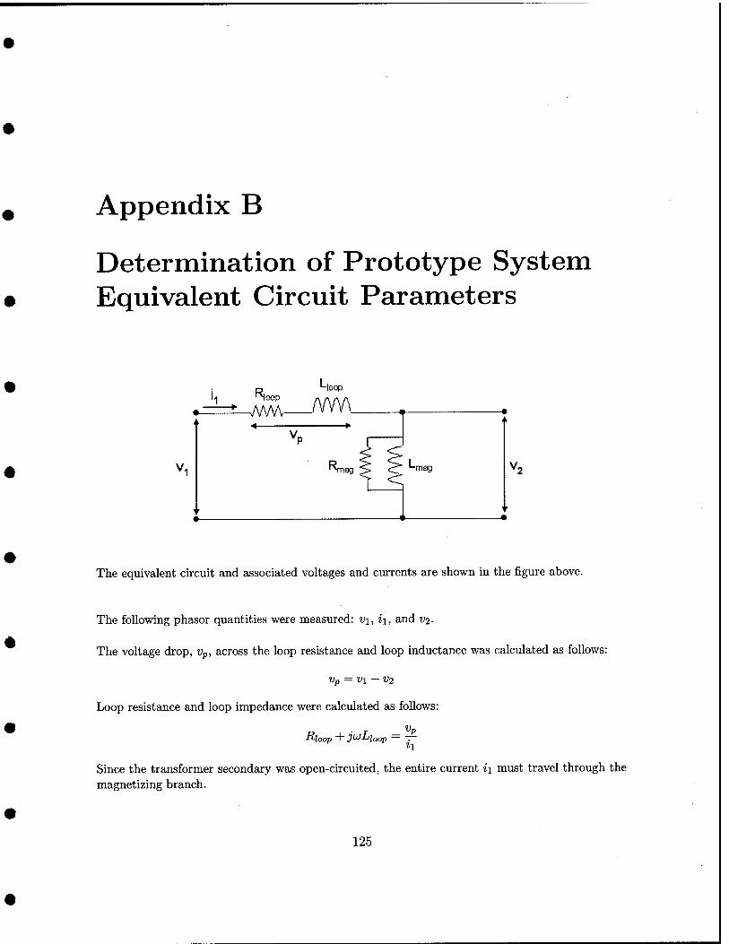
Appendix B
Determination of Prototype System Equivalent Circuit Parameters
1^ r<|oop -loop
:^^^M^- _AAAA_
Rm; ag -mag
The equivalent circuit and associated voltages and currents are shown in the figure above.
The following phasor quantities were measured: vi, ii, and V2.
The voltage drop, Vp, across the loop resistance and loop inductance was calculated as follows:
Vp = Vi- V2
Loop resistance and loop impedance were calculated as follows:
Vp Rloop + j^Lioap = —
Since the transformer secondary was open-circuited, the entire current ii must travel through the magnetizing branch.
125

The equivalent admittance, Ygg, of the magnetizing branch was calculated as follows:
Y -^ '' ~ V2
The magnetizing resistance and magnetizing inductance were then calculated by:
Y^^ = ^ ^_j itmag ^^mag
126
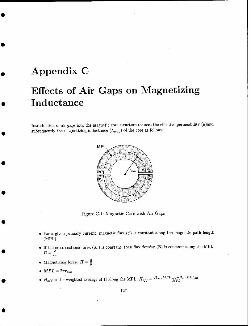
Appendix C
Effects of Air Gaps on Magnetizing Inductance
Introduction of air gaps into the magnetic core structure reduces the effective permeabiUty (/i)and subsequently the magnetizing inductance {Lmag) of the core as follows:
Figure C.l: Magnetic Core with Air Gaps
• For a given primary current, magnetic flux (0) is constant along the magnetic path length (MPL)
• If the cross-sectional area (Ac) is constant, then flux density (B) is constant along the MPL:
• Magnetizing force: H = ^
• MPL = 2'Krave
• Heff is the weighted average of H along the MPL: Heff = tirnrrMPLr.„„.+H„,rMPL^ir
127
e// Effective permeability of the core structure: /ig// = 77
Magnetizing inductance: Lmag = ''"^Cjl+r')'*^^
Example:
ro=4.572cm ri=0.953cm h=15cm /io = 47r * 10~^
f^R,core = 7000
fJ-R,air = 1
For a=0 (i.e., no gap): Lmag = 279.58/^//
For a=lmm: Lmag = 3.37/ii/
The measured value of Lmag (4.507/xH) corresponds to a gap width a=0.745mm.
This gap width matches measurements of the actual prototype core gap.
128

Appendix D
Data From Prototype System Tests
D.l Laboratory Tests
f(Hz) D(m) v1 (volts) ilfA) PF v2 (volls) i2(A) Pin(WO Pout(W) 1
1.00E+03 0.05 0.250 8 0.95 0.140 0.0490 1.78E-01 8.58E-04 0.48%
1.00E+O3 0.05 0.164 4 0.95 0.095 0.0315 7.80E-02 3.74E-04 0.48%
1,D0E-tO3 0.05 0.098 2 0.95 0.060 0.0180 2.33E-02 1.35E-04 0.58%
2.00E-K33 0.05 0.126 6 0.95 0.236 0.0896 8.99E-02 2.64E-03 2.94%
2.[KIE-t03 0.05 0.071 4 0.81 0.160 0.0580 2.87E-02 1.16E-03 4.04%
2.00E+O3 0.05 0.052 2 0.73 0.092 0.0305 9.48E-03 3.51 E-04 3,70%
1.00E-ri34 0.05 1.030 6 0.19 0.450 0.1740 1.45E-01 9.79E-03 6.76%
1.00E404 0.05 0.650 4 0.31 0.286 0.1088 1.00E-01 3.89E-03 3.87%
1.00E-tO4 0.05 0.330 2 0.81 0.192 0.0564 6.67E-02 1.35E-03 2.03%
2.00E-tO4 0.05 1.170 6 0.31 0.472 0.1770 2.71 E-01 1.04E-02 3.85%
2.00E4O4 0.05 0.7B0 4 0.31 0.300 0.1120 1.21E-01 4.20E-03 3.48%
2.00E404 0.05 0.480 2 0.54 0.162 0.0580 6.43E-02 1.17E-03 1.83%
i
i1.00E-tO3 0.25 0.266 6 1.00 0.145 0.0510 2;00E-01 9.24E-04 0.46%
I1.CI0E+O3 0.25 0.170 4 1.00 0.097 0.0325 8.48E-02 3.94E-04 0,46%
'i1.00E-tO3 0.25 0.102 2 1.00 0.055 0.0170 2.55E-02 1.17E-D4 0.46%
i 2.00E-rt]3 0.25 0.180 6 0.99 0.248 0.0940 1.34E-01 2.91 E-03 2.18%
2.00E403 0.25 0.129 4 1.00 0.161 0.0580 6.44E-02 1.17E-03 1.81%
2.0QE-rf)3 0.25 0.075 2 1.00 0.093 0.0310 1.87E-02 3.60E-04 1.93%
1.CI0E-tO4 0.25 0.796 6 0.31 0.330 0.1260 1.84E-01 5.20E-03 2.82%
i1.00E-t€4 0.25 0.560 4 0.31 0.212 0.0780 8.65E-02 2.07E-03 2.39%
i 1.00E-tO4 0.25 0.260 2 0.31 0.120 0.0430 2.01 E-02 6.45E-04 3.21%
1 2.00E+04 0.25 1.270 6 0.31 0.360 0.1360 2.94E-01 6.12E-03 2.08%
! 2.00E+04 0.25 0.824 4 0.31 0.238 0.0880 1.27E-01 2.62E-03 2.06%
1 2.00E-rf)4 0.25 0.452 2 0.31 0.130 0.0470 3.49E-02 7.64E-04 2.19%
1.00E-H33 0.5 0.285 6 1.00 0.145 0.0510 2.14E-01 9.24E-04 0.43%
1.00E-tO3 0.5 0.170 4 0.99 0.100 0.0335 8.43E-02 4.19E-04 0.50%
1.00E-rt)3 0.5 0.088 2 0.99 0.056 0.0170 2.18E-02 1.19E-04 0.55%
2.CI0E+O3 0.5 0.324 6 0.88 0.252 0.0960 2.13E-01 3.02E-03 1.42%
2.00E403 0.5 0.202 4 0.90 0.166 0.0600 9.14E-02 1.25E-03 1.36%
2.00E+03 0.5 0.096 2 0.97 0.092 0.0300 2.32E-02 3.45E-04 1.48%
1.Q0E+O4 0.5 1.010 6 0.31 0.350 0.1320 2.34E-01 5.78E-03 2.47%
1.00E-K34 0.5 0.630 4 0.31 0.224 0.0840 9.73E-02 2.35E-03 2.42%
i1.CI0E+04 0.5 0.334 2 0.31 0.125 0.0450 2.58E-02 7.03E-04 2.72%
2.00E-K]4 Q.5 1.440 6 0.43 0.362 0.1340 4.60E-01 6.06E-D3 1.32%
2.00E404 0.5 0.950 4 0.43 0.242 0.0900 2.02E-01 2.72E-03 1.35%
i 2.00E-K]4 0.51 0.530 21 0.54 0.134 0.0470 7.10E-02 7.87E-04 1.11%
129
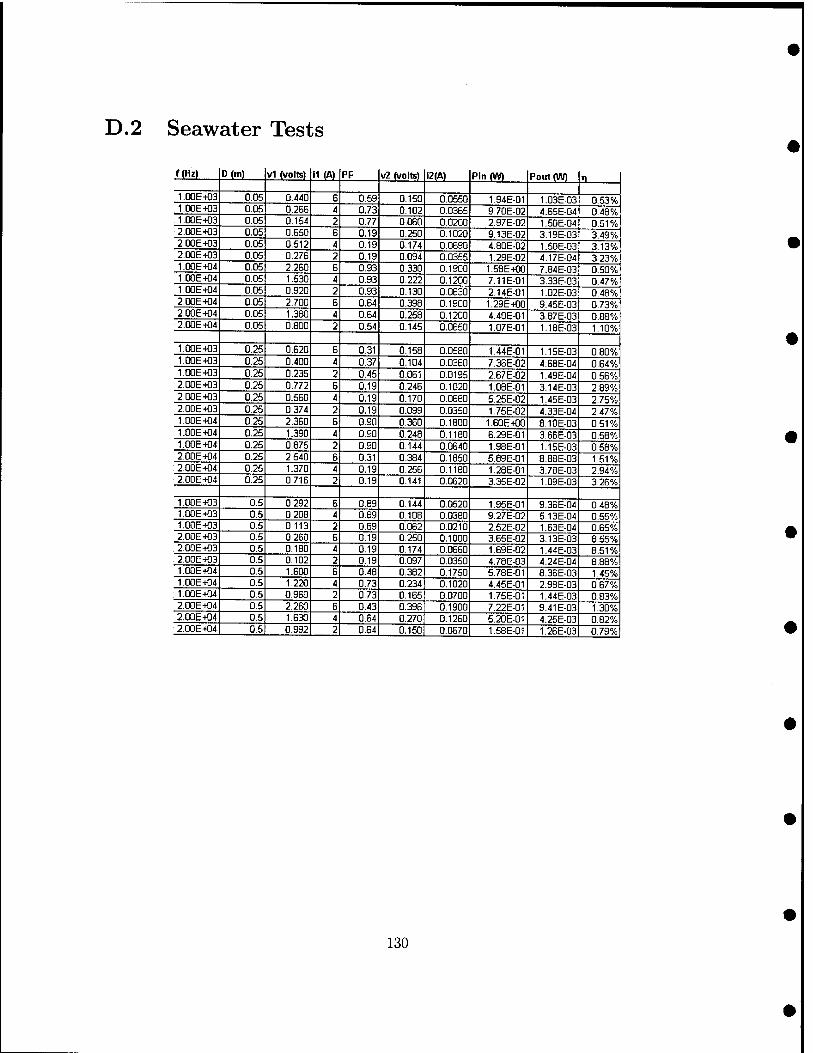
D.2 Seawater Tests
fWt) D(m) v1 (volts) 11(A) PF v2 (volts) 12(A) Pin(VV) Pout(W) »1
1.00E-K)3 0.05 0.440 6 0.59 0.150 0.0650 1.94E-01 1.03E-03 0.53% 1.00E-tO3 0.05 0.266 4 0.73 0.102 0.0365 9.70E-02 4.65E-04 0.48% 1.00E-tO3 0.05 0.154 2 0.77 0.060 0.0200 2.97E-02 1.60E-04 0.51% 2.00E-HD3 0.05 0.650 6 0.19 0.260 0.1020 9.13E-02 3.19E-03 3.49% 2.00E-tO3 0.05 0.512 4 0.19 0.174 0.0690 4.80E-02 1.50E-03 3.13% 2.0OE-tO3 0.05 0.276 2 0.19 0.094 0.0355 1.29E-02 4.17E-04 3.23% 1.00E-tO4 0.05 2.260 6 0.93 0.330 0.1900 1.58E+00 7.84E-03 0.50% 1.00E-HD4 0.05 1,630 4 0.93 0.222 0.1200 7.11E-01 3.33E-03 0.47% 1.00E+04 0.05 0.920 2 0.93 0.130 0.0630 2.14E-01 1.02E-03 0.48% 2,00E+O4 0.05 2.700 6 0.54 0.398 0.1900 1.29E+00 9.45E-03 0.73% 2.00E-tCI4 0.05 1.380 4 0.64 0.258 0.1200 4.40E-O1 3.87E-03 0.88% 2.00E+O4 005 0.800 2 0.54 0.145 0.0650 1.07E-01 1.18E-03 1.10%
1.00E+03 0.25 0.620 6 0.31 0.158 0.0680 1.44E-01 1.15E-03 0.80% 1.00E-tO3 0.25 0.400 4 0.37 0.104 0.0360 7.36E-02 4.68E-04 0.64% 1.DOE403 0.25 0.235 2 0.45 0.061 0.0195 2.67E-02 1.49E-04 0.56% 2.00E+03 0.25 0.772 6 0.19 0.246 0.1020 1.08E-01 3.14E-03 2.89% 2.00E-HD3 0.25 0.560 4 0.19 0.170 0.0680 5.25E-02 1.45E-03 2.75% 2.00E4O3 025 0.374 2 0.19 0.099 0.0350 1.75E-02 4.33E-04 2.47% 1.00E404 025 2.360 6 0.90 0.360 0.1800 1.60E+00 8.10E-03 0 51% 1.O0E-tO4 0.25 1.390 4 0.90 0.248 0.1180 6.29E-01 3.66E-03 0.58% 1.00E404 0.25 0.875 2 0.90 0.144 0.0640 1.98E-01 1.15E-03 0.58% 2.00E-tO4 0.25 2.540 6 0.31 0.384 0.1850 5.89E-01 8.88E-03 151%
; 2.O0E-tO4 0.25 1.370 4 0.19 0.256 0.1180 1.28E-01 3.78E-03 2.94% 2.00E-tO4 0.25 0.716 2 0.19 0.141 0.0620 3.35E-02 1.09E-03 3.26%
1.00E-tO3 0.5 0292 6 0.89 0.144 0.0520 1.95E-01 9.36E-04 0.48% 1.00E-tO3 0.5 0208 4 0.89 0.108 0.0380 9.27E-02 5.13E-04 0.55% 1.00E-tO3 0.5 0.113 2 0.89 0.062 0.0210 2.62E-02 1.63E-04 0.65% 2.00E-K]3 0.5 0.260 6 0.19 0.250 0.1000 3.65E-02 3.13E-03 8.55% 2.00E-rf}3 0.5 0.180 4 0.19 0.174 0.0660 1.69E-02 1.44E-03 8.51 % 2.00E-rf]3 0.5 0.102 2 0.19 0.097 0.0350 4.78E-03 4.24E-04 8.88% 1.00E-tO4 0.5 1.600 6 0.48 0.382 0.1750 5.78E-01 8.36E-03 1.45% 1.00E-rf)4 0.5 1.220 4 0.73 0.234 0.1020 4.45E-01 2.9BE-03 067% 1.0QE404 0.5 0.960 2 0.73 0.165 0.0700 1.75E-01 1.44E-03 0.83% 2,00E-tO4 0.5 2.260 6 0.43 0.396 0.1900 7.22E-01 9.41 E-03 1.30% 2.0QE-tO4 0.5 1.630 4 0.64 0.270 0.1260 5.20E-01 4.25E-03 0.82% 2.00E-*C4 0.5 0.992 2 0.64 0.160 0.0670 1.58E-01 1.26E-03 0.79%
130

Appendix E
Economic Analysis Calculations
E.l Probability and the Normal Distribution
Standard normal distribution:
Z = ^^^ (E.l) a
where:
• Z=standaxd normal variable
• X=actual value
• /i=mean value
• (r=standard deviation
To find a given 95th%:
95th% - n " ^ 1.65
(E.2)
131
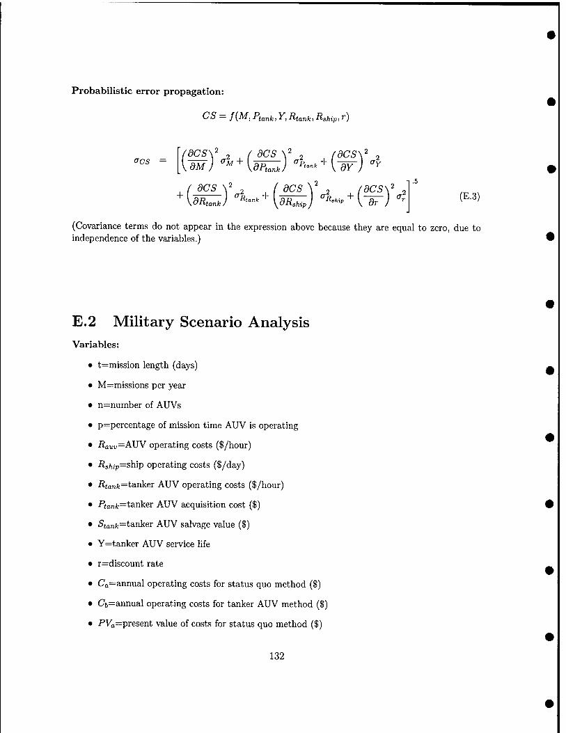
Probabilistic error propagation:
CS = f{M, Ptank, y, Rtank, Rahip, T)
<^CS
/ dcs y" ^ ( dcs V 2 {dcs\'^ ^'^ (E.3)
(Covaxiance terms do not appear in the expression above because they are equal to zero, due to independence of the variables.)
E.2 Military Scenario Analysis Variables:
• t=mission length (days)
• M=missions per year
• n=number of AUVs
• p=percentage of mission time AUV is operating
• i?Qui,=AUV operating costs ($/hour)
• i?s/iip=ship operating costs ($/day)
• /?ianfc=tanker AUV operating costs ($/hour)
• Ptanfc=tanker AUV acquisition cost ($)
• 5tanfc=tanker AUV salvage value ($)
• Y=tanker AUV service life
• r=discount rate
• Ca=annual operating costs for status quo method ($)
• Ci,=annual operating costs for tanker AUV method ($)
• PFa=present value of costs for status quo method ($)
132
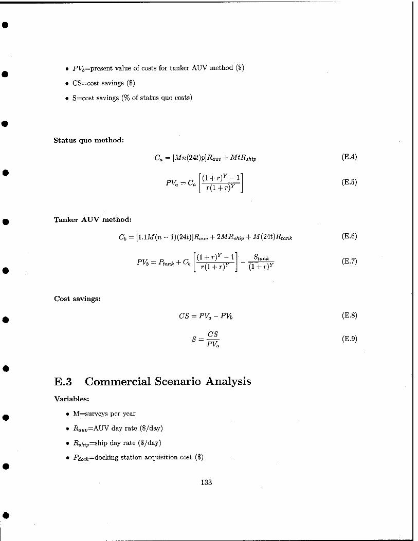
• PFf,=preseiit value of costs for tanker AUV method ($)
• CS=cost savings ($)
• S=cost savings (% of status quo costs)
Status quo method:
Ca = [Mn{2U)p]Rauv + MtRship
'{l + rf-l PVa - Ca
r{l + r)
(E.4)
(E.5)
Tanker AUV method:
Cb = [l.lM(n - l){24t)]Rauv + 2MRship + M{2At)Rtank
PVb = Ptank + Cb (l + r)^-l
r-(l + r) {i + ry
(E.6)
(E.7)
Cost savings:
CS = PVa - PVb
s = CS PVa
(E.8)
(E.9)
E.3 Commercial Scenario Analysis
Variables:
• M=surveys per year
• i?auD=AUV day rate ($/day)
• Rship=ship day rate ($/day)
• -Pdocfc=docking station acquisition cost ($)
133
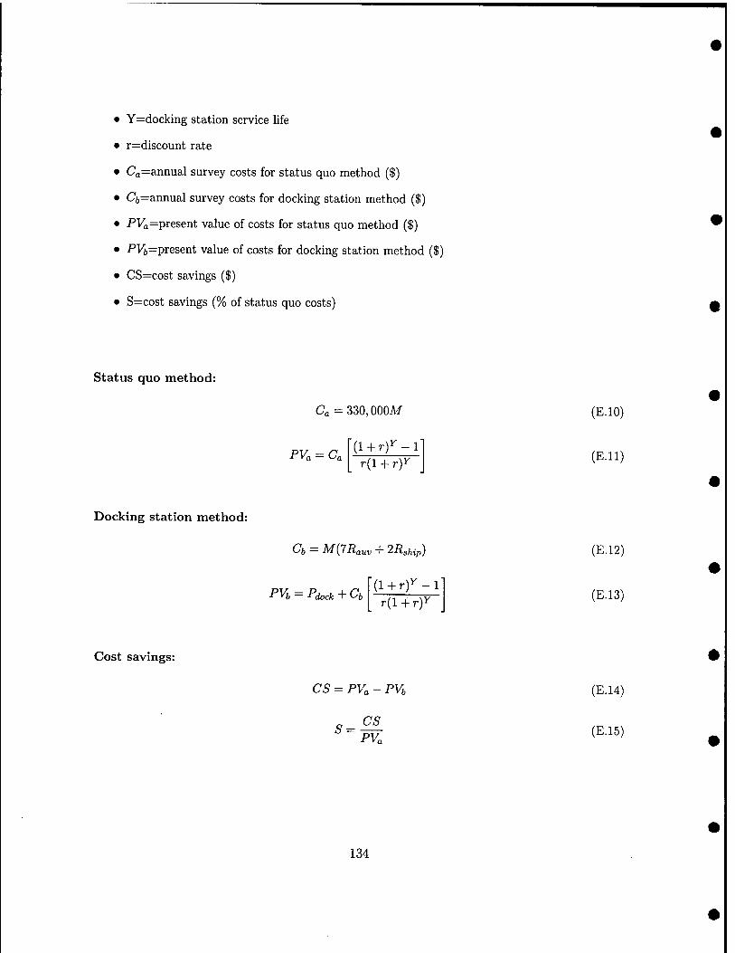
• Y=docking station service life
• rediscount rate
• Ca=annual survey costs for status quo method ($)
• Cb=annual survey costs for docking station method ($)
• PVa=present value of costs for status quo method ($)
• PVb=present value of costs for docking station method ($)
• CS=cost savings ($)
• S=cost savings (% of status quo costs)
Status quo method:
Ca = 330, OOOM
PVa = Ca (l + r)^-l r{l + rY
(E.IO)
(E.ll)
Docking station method:
Cb = M{7Rauv + 2Rship)
'{l + rf -1 ■PH ~ Pdock + Cb
r(l + r)
(E.12)
(E.13)
Cost savings:
CS = PVa - PVb
cs 5-
PVa
(E.14)
(E.15)
134


