ADAPTIVE LONG-PERIOD MULTIPLE ATTENUATION*

ADAPTIVE LONG-PERIOD MULTIPLE ATTENUATION *

BY

H. BRANDSZETER and B. URSIN **

ABSTRACT

BRANDSJETER, H. and URSIN, B., 1979, Adaptive Long-Period Multiple Attenuation, Geophysical Prospecting 27, 709-725.

A least squares estimation procedure is used to estimate the pulse-shape, amplitude function, and arrival time of multiple reflected signals. The estimates of the multiple reflections are subtracted from the data which are subsequently processed by standard methods. The estimation algorithm is applied continuously along the seismic line for each shot point or common datum point. In some cases it is advantageous to apply a pulse-shaping filter prior to using the estimation algorithm.

The effectiveness of the technique is demonstrated by studying common shot point gathers, velocity analyses, and stacked sections derived from field data.

In marine seismic prospecting the data quality is often degraded because of multiple reflections of the water-bottom and water-layer peg-leg multiples, which make interpretation of the seismic sections difficult or impossible. This problem is specially severe in “hard-bottom” areas where the reflection coefficient at the water/sediment interface is large resulting in high amplitude multiple reflections. Hawes (1975) and Taner (1975) have discussed the physical properties of the water-bottom multiples.

Much work has been done in developing methods for the suppression of multiple reflections. The standard data processing techniques, deconvolution (Peacock and Treitel 1969) followed by CDP stacking (Mayne Ig6z), often fail to provide satisfactory attenuation of long-period multiples.

Various types of multichannel filters have been proposed (see, for instance, Schneider, Prince, and Giles 1965, Galbraith and Wiggins 1968, Cassano and Rocca 1973). Assuming a stochastic model of the seismic data, a least squares filter is designed to enhance the primary reflections and to attenuate the multiple reflections. Taner (1975) proposed a multichannel predictive deconvolution filter. Riley and Claerbout (1976) have developed a method based on the scalar wave equation for removing multiple reflected energy from the

* Paper read at the thirty-ninth meeting of the E.A.E.G. at Zagreb, June 1977 ** GECO A.S., Veritasveien I, N-1322 Hovik, Norway.

Geophysical Prospecting ~7 47

710 H.BRANDSBTERAND B.URSIN

seismic data. The use of very long source and receiver arrays has recently proved to be effective in attenuating long-period multiples (Lofthouse and Bennett 1978, Ursin 1978, Moe, Naess, and Aarseth 1977).

The method proposed here is to use a least squares estimation algorithm (Ursin 1979) to compute estimates of the signal pulse, amplitude function, and arrival time of the multiple reflections. The estimated multiples are subtracted from the data which are subsequently processed by standard methods. A similar procedure, using a different estimation scheme, has been proposed by Michon, Wlodarczak, and Merland (1971). A subtraction method based on feedback is discussed by Koehler, Krey, and Wachholz (1974).

In order to have data which satisfy our assumptions more closely we often apply a pulse-shaping filter (Treitel and Robinson 1966) prior to removing the multiples. Both the filtering and the multiple removal will result in improved resolution of the primary reflections in the velocity analysis.

The effectiveness of the algorithm is demonstrated by studying common shot point gathers, velocity analyses and stack sections derived from airgun data and from sparker data.

ESTIMATION ALGORITHM

A mathematical theory of seismic signal detection and parameter estimation has been given by Ursin (1979). The seismic measurements are assumed to consist of a sum of signals corrupted by additive Gaussian white noise uncorrelated to the signals. Each signal is assumed to consist of a signal pulse multiplied by a space-dependent amplitude function and with a space-dependent arrival time. The signal pulse, amplitude and arrival time are estimated by the method of maximum likelihood which is equivalent to the method of least squares for the assumed signal-and-noise model. We shall give a brief description of the estimation algorithm.

The measurement data

m (t, x) = 24 (t, x) + w (t, x) (1)

are given at discrete points x= xj, j = I, 2, . . . , iVl, and at discrete times t =nAt, n= o, I, . . ., N. The spatial variable x may be the receiver location (common shot point data), the source-receiver distance (CDP data) or any other variable according to which the data are classified.

The signal u (t, x) consists of a sequence of K reflected pulses (primary and multiple reflections)

‘U (t,X) = 5 ‘l4k (t, X) = : Uk (X)$k (t- T (Ok, X)), (2) b-1 n-1

where each individual signal %k (t, x) consists of a pulse $k (t) multiplied by

ADAPTIVE LONG-PERIOD MULTIPLE ATTENUATION 711

an amplitude function ak (x) and with a variable arrival time T (Ok, x). It is assumed that the arrival times can be given a parametric representation so that each arrival time function is a fixed function T (0, x) of x and a parameter vector 0 which has at least two components, the two-way travel time and the stacking velocity. The signal pulses are assumed to be of finite duration so that $k (nAt) # o only for n = o, I, . . . , L. The pulse duration LAt is assumed to be small compared to the duration of the measurement NAt. It is also assumed that the signals uk (x) $k (t - T (Ok, x)) do not overlap, so that at any point in the T-x-plane there is only one signal present.

Each individual signal Uk (t, x) will remain unchanged if we divide the amplitude function ak (x) by a constant and multiply the signal pulse $k (t) by the same constant. In order to get ak (x) and $k (t) uniquely defined we need a normalization procedure, and we have chosen to normalize so that a (x1) = I. The noise w (t, x) is assumed to be white Gaussian noise with zero mean value. It is also assumed that the noise is uncorrelated to the signal.

An estimate of the signal is denoted by

dk (6 X) = dk (x) Sk (t- T ($k> X)), (3)

where $k (t) and 6k (x) are estimates of the signal pulse and amplitude function, and ok is an estimate of the arrival time parameter vector.

In the method of least squares we minimize the error function (which depends on 6k) :

I = z i {m(nAt+T(h k, xj), xj) - kk (%) $k (nAt))2. (4) f-1 IS-II

The least squares estimates of LZk (~j) and $k (nht) satisfy the equations

31

3kk (xj) = 2 & (“j) i & (nAt)z

n--O

- 2 i m (nAt + T (@k, xj), xj) $k (nAt) = 0 n-0

(54

31 __~ @k (sat)

= 2 & (nAt) ; & (Xj)z j=1

- 2 : WZ (nht + T (&, Xj), Xj) ‘ik (Xj) = 0. (5b) j-1

These equations are solved iteratively by alternately keeping L$k (%j) and p”k (IzAt) fixed.

From (5a) we see that the estimate of the signal amplitude at XJ is proportional to the crosscorrelation coefficient between the measurement at xj (that is, trace number j) and the estimate of the signal pulse.

712 H.BRANDSzETERAND B.URSIN

In order to obtain improved estimates of the arrival times we let the estimated arrival time of each signal be given by

?-k (q) = T (6 k, xj) + ATk (q)> (6)

where ATk (XJ) is a correction term (residual normal moveout). These correction terms are computed so that the correlation between the measurement and the estimate of the signal pulse is maximum.

The new estimate of the signal amplitude is proportional to the maximum value of the crosscorrelation function. Since dk (xl) = I, we have that the estimate of the signal amplitude at xj is equal to the maximum value of the crosscorrelation function at xj divided by the maximum value at xl.

The new estimate of the signal pulse is obtained from (5b) which gives

ii! VP2 (+zAt+?k (Xj), Xj) & (Xj)

$k (flat) = ,=1

5 dk (xj)” (7)

In order to start the computations we need initial values of the estimates of the signal parameters. We use a constant amplitude function, & (xj) = I, j=I, . ..) M, and obtain an estimate of the arrival time parameter vector from a velocity analysis.

There are two ways to terminate the algorithm. The computations are stopped if the number of iterations exceeds a given number or if the change in the coherency measure used is below a given value. We use the semblance coefficient which, for the assumed signal-and-noise model, is given by Ursin

(1979) :

5 dk (Xj)2 i & (aAt)2

s = ‘-I n=o ii i! m (%ht+?!-k (q), xj)”

(8)

The final step of the algorithm is to subtract the estimated multiple reflections from the data. The algorithm is applied continuously along the seismic line to each shot point or CDP gather.

For the reflected signals not to overlap the duration of the signal pulse should be small. This may not be so due to the presence of bubble pulses. In that case we apply the estimation algorithm to a single reflection which does not interfere with any other event. The estimated signal pulse is used in the design of a pulse-shaping filter which is applied to the data before the removal of the multiple reflections.


APPLICATION TO FIELD DATA

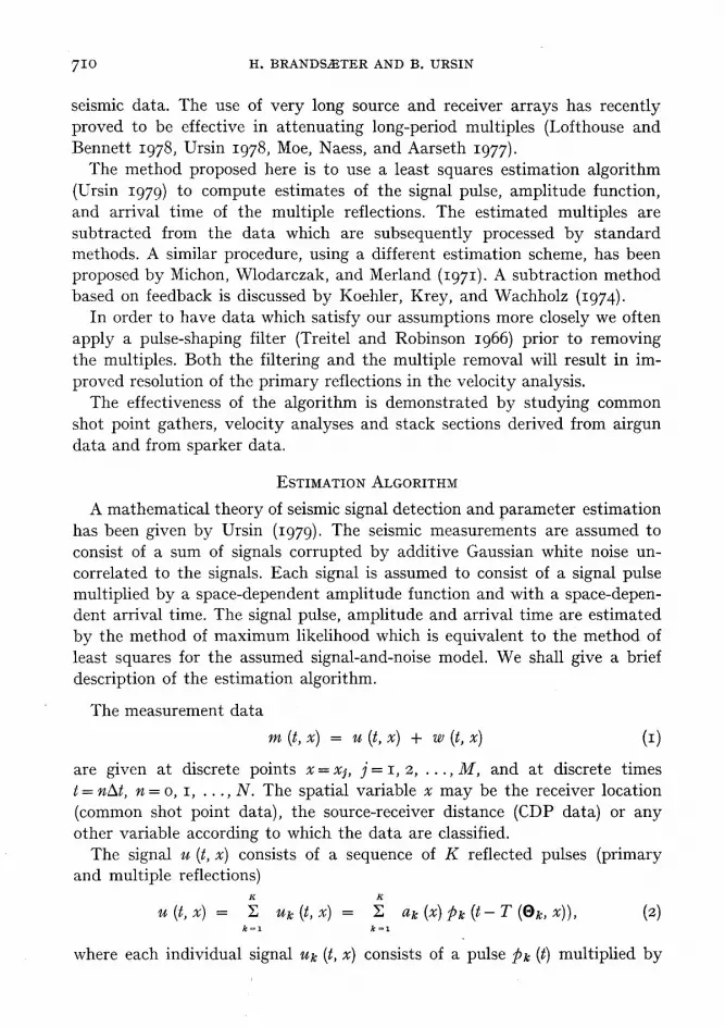
The effect of applying the multiple attenuation program to field data will be shown in two examples, one with airgun data and another with sparker data.

Airgun data

Fig. I shows a near-trace section recorded offshore Norway with a 32.8 1 (zoo0 cuin.) airgun array. The amplitudes of the water-bottom multiples are very strong. The peg-leg multiples from the upper layers and the long pulse duration make the situation even more complicated. Fig. 2 shows the same near-trace section after the application of a pulse-shaping filter. The filter is computed from an estimate of the first water-bottom multiple. The desired output pulse is a delayed zero-phase pulse. In fig. 3 the filtered data are shown after two steps of multiple removal. First the water-bottom multiples were estimated and subtracted from the data, and then the process was repeated for the peg-leg multiples.

In order to enhance the events just beneath the seafloor, the water-bottom reflection has been estimated, and half of the estimated signal has been subtracted from the data.

SP 0

1 50 100 150 200 250 300 350 400 450 500 550 600 650

Fig. I. Near-trace section of field data.

714 H. BRANDSlETER AND B. URSIN

SP 1 5-O 100 150 200 250 300 350 LOO 450 500 550 600 650

SP 0

Fig. 2. Near-trace section after the application of a pulse-shaping filter.

7 50 loo 150 200 250 300 350 400 60 500 550 600 650

Fig. 3. Near-trace section after the removal of multiple reflections.


I I ‘VII I I 1 i.( 1, ‘. I

Fig. g. 24 fold CDP stack.

SP 1 50 100 150 200 250 300 350 400 450 5W 550 GO0 650 700 750 800

3

Fig. IO. 24 fold CDP stack, after multiple removal.

05

10

15

-05

.lO

-15

Fig.

I I.

Deta

il A,

co

nven

tiona

l pr

oces

sing.

Fig.

12.

Deta

il A,

aft

er

multip

le re

mova

l.


ADAPTIVE LONG-PBRIOD hfUL.?‘IPLE ATTENUATION

o,o-

0.2-

O,L-

O,G-

0.8-

Fig. 17. Shot-point data, before and after the removal of multiples (the far-trace is recorded twice).

STAC

KING

VE

LOCI

TY

I M/S

EC

I ST

ACKI

NG

VELO

CITY

IM

/S

EC

I

0.8

Fig.

18.

Veloc

ity

analy

sis

of fie

ld da

ta (sh

own

in fig

. 17

”).

i ’

Fig.

IQ.

Veloc

ity

analy

sis

of da

ta aft

er

multip

le re

mova

l (sh

own

in fig

. I

7b).

N * ‘9 0 P P i I


724 8. BRANDSBTER AND B. URSIN

The effect of the data processing on a shot point record is shown in figs. 4 and 5. Fig. 4a shows the field data, and fig. 4b shows the same data after the application of the pulse-shaping filter. In fig. 5a we see the data after the removal of the water-bottom multiples, and in fig. 5b the peg-leg multiples have also been removed.

The corresponding velocity analyses are shown in figs. 6-8. Fig. 6 shows the velocity analysis of the field data, and in fig. 7 we see the velocity analysis of the filtered data. Fig. 8 shows the velocity analysis after multiple removal.

Using standard data processing methods we obtain the twenty-four fold stack section shown in fig. 9. Applying the same data processing to the data from which the multiples have been removed, results in the section shown in fig. 10.

An enlarged view of the details marked A in figs. 9 and IO is shown in figs. II and 12. On the multiple attenuated section there is an event between 1.0 s and 1.1 s which is concealed by the multiple energy on the standard section.

The details marked B are shown enlarged in figs. 13 and 14. The multiple reflections have been attenuated, thus improving the continuity of the dipping events.

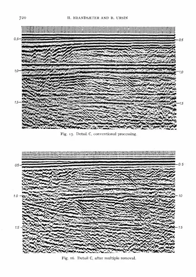
Figs. 15 and 16 show an enlarged view of the details marked C. The dipping events which start at 0.7 s and 1.1 s to the left in fig. 16 can hardly be seen on the conventionally processed section shown in fig. 15.

Sparker data The multiple attenuation program has also been applied to high-resolution

sparker data. The data were recorded with I ms sample interval on eleven data channels, each channel being the output from a 25 m section of the hydrophone cable.

Fig. 17 shows shot point data before and after multiple removal. Three water-bottom multiples and two peg-leg multiples of the event at 0.5 s have been removed.

Figs. 18 and rg show the velocity analyses of the shot point records shown in fig. 17. The multiple energy has been reduced, resulting in improved quality of the velocity analysis.

An eleven fold stack section of the sparker data processed by conventional methods is shown in fig. 2.0. Fig. 21 shows the same data after multiple removal. Two events, at 0.62 s and 0.74 s to the left in fig. 21, appear on the multiple- attenuated section. These events can hardly be seen on the conventional section. The event at 0.61 s in fig. 20 is a multiple reflection of the event at 0.35 s.

Documents

ADAPTIVE LONG-PERIOD MULTIPLE ATTENUATION*