Proceedings of the ASME 2011 30th International Conference on Ocean, Offshore and Arctic Engineering OMAE2011

June 19-24, 2011, Rotterdam, The Netherlands

OMAE2011-50275

ESTIMATORS OF WAVE PEAK PERIOD FOR LARGE RETURN PERIOD SEASTATES

Michele Drago, Tiziana Ciuffardi, Giancarlo Giovanetti Saipem Energy Services

OCEAN department Fano (PU), Italy

Michele.drago@saipem.eni.it

ABSTRACT Different functional relationships for the distribution of the

peak period Tp for a given seastate Hs are tested against hindcasted and measured time series for various locations in the European seas, namely Barents Sea, Baltic Sea and Western Mediterranean (Tyrrhenian) Sea. The aim is to investigate their performance when extrapolating from available data for the estimation of the long return period seastates which are not covered by the length of the time series.

A second complementary objective of the paper is to quantify the uncertainty and the variability that can occur in the estimation of the Hs/Tp association when a short time series is available. This is done by assessing the Hs/Tp relation from a 35-years long time series that will be considered as the correct one. Then it will be compared with those obtained by analysing multiple cases of shorter and shorter portions of the time series. The spread of the results against the one obtained with the entire time series will be estimated to give some indications about how long a time series has to be to ensure a correct extrapolation to the long return period seastates and to provide an indication of the error that can affect the results when a short time series is available.

INTRODUCTION The estimation of the peak period Tp to be associated to an

extreme seastate Hs is often an underestimated issue. In fact, main accuracy is focused in the evaluation of the significant wave height in extreme seastate, leaving to a ‘second order’ importance the associated Tp.

Actually, in certain problems, the correctness of the peak period Tp has a relevance even larger of the Hs accuracy as an

uncertainty in the order of one second could cause a large difference in the results of the analyses. Typical examples are the ringing of tension leg platforms (TLP) and vessels seakeeping behaviour where the heave, pitch and roll responses at the respective natural resonant frequencies could be excited or not by small differences in the frequency of the wave cyclic load forcing (Faltinsen, [1]).

Many standard relationships can be found for the estimation of the mean peak period range to be associated to extreme seastates (DNV, [2], Carter et al., [3]). Furthermore, numerous semi-empirical relations, as the SMB (Sverdrup-Munk-Bretschneider) method, are sometimes used in wave prediction to link the significant wave height Hs and wave peak period to wind speed, fetch, and water depth (Bretschneider [4], CERC [5]). These methods can be used as thumb rules to derive the wave peak period related to significant wave height.

Nevertheless, a reliable definition of the mean peak period to be associated to an extreme seastate and of its distribution can only derive from a rigorous statistical analysis of a database of simultaneous significant wave height/peak period values, measurements or hindcasting, specifically acquired/developed for the location of interest. Different models can be applied for the probabilistic analysis of simultaneous environmental variables. Among the others it is worthwhile to mention the Maximum Likelihood Model (MLM) (Prince-Wright, [6]) and the Conditional Modelling Approach (CMA) (Bitner-Gregersen and Haver, [7]), which is the one adopted in the present paper. The CMA model defines the joint density function of two environmental variables, Hs and Tp for the present case, in terms of a marginal distribution of Hs and a series of density distributions of Tp conditional on Hs. The selection of the most

1 Copyright © 2011 by ASME

appropriate functional relationship between the marginal variable Hs and the parameters of the conditional distributions has a crucial role for a proper estimation of large return period events, i.e. when extrapolating the data, as the use of different relationships can lead to substantially different results.

However, even the rigorous treatment of the data and the selection of the most appropriate function are not sufficient to guarantee a reliable result when extrapolating to large return period events. In fact, it is necessary also that a sufficiently large population of Hs-Tp couples is available for all the Hs classes for which a conditional Tp distribution shall be specified. This is rarely true for larger measured Hs classes when short time series are available.

This requirement is more stringent than the one for the definition of the marginal distribution of Hs, where all the values of the dataset can be used. Hence, even if a time series is long enough for a proper estimation of the significant wave height Hs, it could not provide sufficient information for a reliable estimation of the peak period Tp. Therefore, for a reliable estimation of Tp, a certain duration of the dataset is necessary. Generally, this makes hindcasting data much more suitable for the scope as measurements specifically collected for a certain location, when available, rarely exceed few years and often present a too short duration.

METHODOLOGY Following the CMA model (Bitner-Gregersen and Haver,

[7]), the seastate climate can be defined by a joint probability density function of the significant wave height Hs and the spectral peak period Tp that in a general form can be written as

( TpHsf TpHs ,, )

( ) ( ) ( )HsTpfHsfTpHsf HsTpHsTpHs ⋅=,, (1)

where is the marginal probability distribution of the significant wave height Hs and

( )Hsf Hs

( )HsTpf HsTp is the probability

distribution of the spectral peak period Tp, conditional on the significant wave height Hs.

The present paper is focused on the estimation of the probability distribution of the spectral peak period

( )HsTpf HsTp , hence no emphasis will be given to the various

marginal probability distributions that can be used. ( )Hsf Hs

It is sufficient to mention that for the Barents Sea and Baltic Sea cases the LONOWE marginal probability distribution has been used (Haver, [8]), while for the Tyrrhenian Sea the 3-parameters Weibull distribution has been adopted (Carter et al. [3].

Whatever the adopted is, the distribution of the peak period Tp for any seastate Hs is well described by the log-normal distribution (Haver and Nyhus, [9], Bitner-Gregersen [10]).

( )Hsf Hs

( )( )

( )[ ]( ) ⎪⎭

⎪⎬⎫

⎪⎩

⎪⎨⎧ −−= 2

2

2lnexp

21

HsHsTp

TpHsHsTpf HsTp σ

μπσ

(2)

The parameters μ and σ define, for each Hs value, the log-

normal distribution, and consequently also its mean value

( )2exp)( 2σμ +=meanTp (3)

that is usually associated to any Hs for design calculation. The log-normal parameters are easily computed from an available seastate dataset for not extreme seastate conditions by fitting technique for any Hs class with a sufficient population. On the contrary, the evaluation of the peak period distribution and of its mean value for large return period seastates, which are not covered by the dataset, requires an extrapolation of the parameters μ and σ that define the log-normal distribution.

This is generally done by fitting the functions ( )Hsμμ = and ( )Hsσσ = to the available values obtained by log-normal

distribution on seastates classes significantly represented in the dataset, and then extrapolating them to larger Hs values not covered or scarcely covered by the dataset. The selection of different extrapolating functions can bring to very different results for seastates with return period much longer than the available seastate time series duration, potentially with large effect on off-shore structures design. Hence, in many cases, a correct estimation of the peak period distribution and of its mean value for long return period seastates is essential for a safe and reliable design.

In the present paper, different functions ( )Hsμμ = and

( )Hsσσ = are tested against available measured and hindcasted time series for various locations in some European seas. The considered time series are listed and briefly described in Tab. 1, where the abbreviation “Hind” refers to hindcasted data, while “Ron” refers to Rete Ondametrica Nazionale (Italian National Wave Network) buoy measured data.

Tab. 1: Brief description of analyzed locations. Location Lat (°N) Lon (°E) WD (m) Period (y) Time step (h) Kind

Barents Sea 71.377 22.804 385 35 3 HindBaltic Sea 58.570 20.130 60 27 1 Hind

Tyrrhenian Sea 43.919 9.818 100 13 3 Ron

Fig. 1, Fig. 2 and Fig. 3 show respectively the location of the Barents Sea time series (NEXT-RA database, Oceanweather USA [11]), of the Baltic Sea time series (BALSEA database, Danish Hydraulic Institute, Denmark [12]) and of the Tyrrhenian Sea time series (Rete Ondametrica Nazionale buoy, Italy [13]).

2 Copyright © 2011 by ASME

Sweden

Norway

North Sea

Barents Sea

Finland

Russia

Sweden

Norway

North Sea

Barents Sea

Finland

Russia

Fig. 1: Location of Barents Sea time series.

Sweden

Norway

Baltic SeaDenmark

Sweden

Norway

Baltic SeaDenmark

Fig. 2: Location of Baltic Sea time series.

ItalyFrance

Corsica

Tyrrhenian Sea

ItalyFrance

Corsica

Tyrrhenian Sea

Fig. 3: Location of Tyrrhenian Sea time series.

The following functions are tested. For ( )Hsμμ = : Power function (Bitner-Gregersen [10]) a) 3-parameters (4) 31

2 aHsa a +=μ

b) 2-parameters (5) 21

aHsa=μ

Arctangent function (Haver, [8])

( )[ ]321 arctan aHsaa +=μ (6) μ-Haver function (Haver, [14], Jonathan et al., [15])

( ) ( ) 322

1 1ln1 aHsaHsa ++++= −μ (7) For ( )Hsσσ = : Exponential function (Bitner-Gregersen [10]) a) ( )Hsaa 21

2 exp −=σ 2-parameters (8)

b) ( ) 3212 exp aHsaa +−=σ 3-parameters (9)

σ-Haver function (Haver, [14], Jonathan et al., [15])

312 2 aHsa a +=σ (10)

From now on in the paper, the various functions will be

identified by the above bold characters names. For both ( )Hsμμ = power function and ( )Hsσσ =

exponential function it is distinguished between the 2 and 3-parameters cases as they have peculiar influences for large Hs cases, influencing the Tp mean value and its range associated to any probability level.

It should be noted that when dealing with the mean peak period associated to extreme waves, the most important parameter is the μ parameter, as tends to be negligible when moving toward large Hs.

2σ

On the contrary, is a more relevant parameter when defining the confidence interval of the peak period associated to an extreme Hs or the Tp values to be associated to a certain Hs when defining the iso-probability contours in the Hs-Tp space.

2σ

For example, for the estimation of the 90% confidence interval of the peak period, the following relationships hold:

( )σβμ 2exp%5 −=Tp , ( )σβμ 2exp%95 +=Tp , (11)

with β=1.165. More generally, for any confidence interval α, β can be calculated by integrating the error function

( )βα erf+=21

2 (12)

with σ

μβ

2ln −

=Tp .

Iso-probability contours are implicitly defined by the joint probability density function . In fact, it assigns to each seastate a probability density: fixing the probability

( TpHsf TpHs ,, )

3 Copyright © 2011 by ASME

density associated to any extreme Hs-Tp seastate couple, seastates couples with lower significant wave height but spectral peak period longer or shorter than the mean peak period that have the same probability density can be defined. Hence, in the Hs-Tp space, contour lines passing through all the points having the same probability density of the Hs extremes with any return period can be developed. The Tp range corresponding to each Hs can be calculated by the error function (eq. 12), hence strictly depends on the value of . 2σ

DIFFERENT ESTIMATORS PERFORMANCE Fig. 4 to Fig. 6 and Fig. 11 to Fig. 13 show respectively the

( )Hsμμ = and the (Hs)σσ = fittings for the various cases. It can be noted that all the various fitting functions perform similarly when interpolating the Hs classes of the dataset covered by a sufficient number of cases, but substantial differences can be found when extrapolating from the higher available Hs class.

To be noted that larger Hs included in the datasets have not been considered in the fitting as too few data fall in the correspondent Hs classes to allow a reliable definition of the log-normal distribution. Therefore, the goodness of extrapolation can be evaluated looking how the various functions fit the upper tail of the Hs/Tp couples (see Fig. 7 to Fig. 9).

Tab. 2 reports the highest Hs class used for ( )Hsμμ = and (Hs)σσ = fittings for each case and the maximum Hs included

in the datasets. Tab. 2: Maximum Hs class used for fitting procedure and

maximum Hs values included in datasets. Barents Sea Baltic Sea Tyrrhenian Sea

Variable Hs class (m) Hs data (m) Hs class (m) Hs data (m) Hs class (m) Hs data (m)μ 10.500 14.077 6.625 8.156 5.750 6.600σ 10.500 14.077 5.625 8.156 4.250 6.600

Comparing (Hs)μμ = functions, a general behavior of the various functions when extrapolating to large can be observed. Three main conclusions can be drawn:

Hs

a) Arctangent function always provides the lower μ values. This is a logical consequence of the fact that the function is the only one asymptotically limited on the upper side.

b) Power 3-parameters and μ-Haver functions perform very similarly and provide intermediate μ value.

c) Power 2-parameters function always provides the larger μ value.

Barents Sea: μ fitting functions

1.6

1.8

2.0

2.2

2.4

2.6

2.8

3.0

0.0 2.0 4.0 6.0 8.0 10.0 12.0 14.0 16.0 18.0 20.0

Hs (m)

μ

μ=arctan(3p)μ=power(3p)μ=power(2p)μ=haver(3p)Best fit values

Fig. 4: Barents Sea μ fitting functions.

Baltic Sea: μ fitting functions

1.0

1.2

1.4

1.6

1.8

2.0

2.2

2.4

2.6

0.0 1.0 2.0 3.0 4.0 5.0 6.0 7.0 8.0 9.0 10.0

Hs (m)

μ

μ=arctan(3p)μ=power(3p)μ=power(2p)μ=haver(3p)Best fit values

Fig. 5: Baltic Sea μ fitting functions.

Tyrrhenian Sea: μ fitting functions

1.4

1.6

1.8

2.0

2.2

2.4

2.6

0.0 1.0 2.0 3.0 4.0 5.0 6.0 7.0 8.0 9.0 10.0

Hs (m)

μ

μ=arctan(3p)μ=power(3p)μ=power(2p)μ=haver(3p)Best fit values

Fig. 6: Tyrrhenian Sea μ fitting functions.

Recalling equation (3), the above conclusions are reflected

by the resulting ( ) ( )( HsHsTpmeanTp )σμ ,)( = curves reported in Fig. 7 to Fig. 9 together with the dataset points for the three considered cases. Moving to large the mean peak period

is more and more dependent only on the increasing Hs

Tp μ value and less on the decreasing σ value. Hence, in this figures, the influence of σ on the Tp value has not been explored. The ( )Hsσσ = σ-Haver function has been used in combination with the various ( )Hsμμ = functions for uniformity in comparison.

4 Copyright © 2011 by ASME

Fig. 7: Comparison between several combinations of fitting

functions for Barents Sea case study.

Fig. 8: Comparison between several combinations of fitting

functions for Baltic Sea case study.

Fig. 9: Comparison between several combinations of fitting

functions for Tyrrhenian Sea case study.

Even if a rigorous assessment on the absolute performance of the various fitting functions has not been developed, it is possible to visually observe that:

a) The arctangent fitting function generally

underestimates the peak period, at least for the considered cases.

b) The μ-Haver and 3 parameter power functions provide the best fit for the Baltic and, even if less clearly, for the Tyrrhenian Sea, while the 2-

parameters power function tends to overestimate for these datasets.

c) The 2-parameters power function provides the best fit for the Barents Sea case, the other functions tend to underestimate.

Tab. 3 to Tab.5 report for the 1, 10 and 100-years return

period Hs the associated mean peak period Tp obtained by the best fitting function and by the other functions with the resulting percentage difference. It can be observed that the differences are not negligible.

Tab. 3 : Barents Sea – Comparison of Tp resulting by the different

functions Return Power (2p) Power (3p) Haver Arctangent period (y) Hs (m) Tp (s) Err (%) Tp (s) Err% Tp (s) Err % Tp (s) Err %

1 10.62 14.43 ------ 14.13 2.09 14.14 2.04 13.82 4.2310 13.15 15.63 ------ 15.08 3.52 15.11 3.36 14.38 8.00100 15.59 16.70 ------ 15.89 4.83 15.94 4.52 14.79 11.44

Tab. 4 : Baltic Sea – Comparison of Tp resulting by the different

functions Return Power (3p) Power (2p) Haver Arctangent period (y) Hs (m) Tp (s) Err (%) Tp (s) Err% Tp (s) Err % Tp (s) Err %

1 6.63 10.54 ------ 10.81 2.61 10.48 0.53 10.29 2.3210 8.17 11.42 ------ 11.99 5.01 11.29 1.12 10.76 5.81100 9.68 12.20 ------ 13.09 7.31 12.00 1.62 11.09 9.05

Tab. 5 : Tyrrhenian Sea – Comparison of Tp resulting by the

different functions Return Power (3p) Power (2p) Haver Arctangent period (y) Hs (m) Tp (s) Err (%) Tp (s) Err% Tp (s) Err % Tp (s) Err %

1 5.39 10.27 ------ 10.38 1.04 10.25 0.22 10.14 1.2810 6.81 11.05 ------ 11.26 1.90 10.98 0.61 10.63 3.83100 8.21 11.72 ------ 12.04 2.70 11.61 0.95 10.97 6.38

In general, it can be concluded that, to obtain a good result,

various fitting functions should be tested and compared against the dataset. Trying to extrapolate a general rule, it can be observed that the 2-parameter power function, the one resulting in longer peak periods Tp, provides the best agreement with the data for large Tp to Hs ratio (Barents Sea), while for intermediate Tp to Hs ratios 3-parameters power and μ-Haver functions are the better performing. Therefore, the selection of the most appropriate function could be related to the considered metocean ambient, i.e. to the length of the fetch along which the seastate can develop, longer fetches allowing the development of longer periods (CERC, [5]).

This could also mean that the arctangent function could be the best performing for low Tp to Hs ratio. Many other test cases shall be considered to verify this hypothesis. Fig. 10 shows an example of the division of the Hs-Tp space in different range of validity of ( )Hsμμ = functions that could be obtained. Obviously numerical values of limiting curves are not trustworthy, but it is interesting to note that Hs-Tp curves seem to follow a relationship of the type 31HsTp α= instead of the usually adopted 21HsTp α= .

5 Copyright © 2011 by ASME

Analyzed locations: Tp (Hs)

0

2

4

6

8

10

12

14

16

0 2 4 6 8 10 12 14 16 18

Tp (s)

Hs

(m)

Barents SeaBaltic SeaTyrrhenian Sea

Tp=6.2Hs0.333Tp=5.3Hs0.333

2-p power

3-p power μ-Haver

Arctangent ?

Fig. 10 : Hs-Tp space with attempt of definition of range of

validity for ( )Hsμμ = functions For what regards the (Hs)σσ = functions, it can be observed a different behavior between the three considered cases (Fig. 11 to Fig. 13). The following conclusions can be made:

a) Being the only one asymptotically limited to a lower value different from zero, the exponential 3-parameters function generally leads to larger σ values, but this is not true for the Tyrrhenian Sea case (Fig. 13).

b) The exponential 2-parameters function, even if it has a zero asymptotical limit like the σ-Haver function, could decrease too rapidly on respect to the fitting points. Its lower flexibility is a direct consequence of the use of only two fitting parameters

c) The behavior of the various functions is more dependent on the case by case fitting, but the one always ‘correctly’ fitting the data points is the σ-Haver function.

The performance of the various (Hs)σσ = functions is

verified by comparing the resulting iso-probability curves of the Barents Sea and Baltic Sea cases with the Hs-Tp points of the relevant dataset (Tyrrhenian Sea case is not considered as all functions perform similarly and no differences are appreciable in the iso-probability contours).

For the Barents Sea and Baltic Sea cases, the contour lines

associated with the 35-years (Barents Sea) and 27-years (Baltic Sea) return periods probability and for different σ fitting functions are reported respectively in Fig. 14 and Fig. 15. This test is devoted to evaluate the performance of the various

(Hs

Barents Sea: σ fitting functions

0.00

0.05

0.10

0.15

0.20

0.25

0.30

0.0 2.0 4.0 6.0 8.0 10.0 12.0 14.0 16.0 18.0 20.0

Hs (m)

σ

σ=exp(2p)σ=exp(3p)σ=haver(3p)Best fit values

Fig. 11: Barents Sea σ fitting functions

Baltic Sea: σ fitting functions

0.00

0.05

0.10

0.15

0.20

0.25

0.0 1.0 2.0 3.0 4.0 5.0 6.0 7.0 8.0 9.0 10.0

Hs (m)

σ

σ=exp(2p)σ=exp(3p)σ=haver(3p)Best fit values

Fig. 12: Baltic Sea σ fitting functions

Tyrrhenian Sea: σ fitting functions

0.00

0.05

0.10

0.15

0.20

0.25

0.30

0.35

0.0 1.0 2.0 3.0 4.0 5.0 6.0 7.0 8.0 9.0 10.0

Hs (m)

σ

σ=exp(2p)σ=exp(3p)σ=haver(3p)Best fit values

Fig. 13: Tyrrhenian Sea σ fitting functions

)σσ = functions; hence only the best (Hs)μμ = cases, i.e. the power 2 parameters function for the Barents Sea and the power 3 parameters function for the Baltic Sea are considered.

Fig. 14: Barents Sea: 35-years return period iso-probability contour lines.

6 Copyright © 2011 by ASME

Fig. 15: Baltic Sea: 27-years return period iso-probability contour

lines. For the Barents Sea all the fitting functions have the same

behavior with only small differences. As for the Tyrrhenian Sea case it can be concluded that any one of the fitting functions could be adopted.

Differently, for the Baltic Sea, the various functions provide rather different results. The 2 parameters exponential function seems the one in better agreement with the dataset but, also looking at the fitting in Fig. 12, it could be expected that it provides a too narrow range for large Hs. The 3 parameters exponential function seems to provide a too wide range and therefore is over-conservative. The right compromise between accuracy and conservativeness seems to be the σ-Haver function. In this sense the σ-Haver function seems to be the one providing the better result for all the three cases.

Anyway, like for the ( )Hsμμ = functions, the decision about the fitting function to be selected should be taken after the testing of various functions by comparison of the results with the dataset points.

TIME SERIES DURATION VS. PEAK PERIOD ESTIMATION RELIABILITY

For this analysis, the 35-years long time series of the Barents Sea has been used. Beside the analysis of the whole time series, which has been considered the ‘correct’ one and used for comparison, 1-year, 5-years and 10-years long portions of the time series have been analyzed.

Five different time series portions have been selected for 1-year (casually) and 5-years (partially overlapping) long cases. Three time series (partially overlapping) portions have been selected for the 10-years long case.

The relationships providing the best estimate for the whole time series case, i.e. the 2 parameters power function for the μ parameter (eq. 4) and the 2 parameters exponential function for the σ parameter (eq. 7), are assumed as the ‘correct’ ones. Hence, they have been applied also for the analyses of the shorter time series portions and the related results for the 35-years long time series used for a quantitative comparison.

Tab. 6 shows, for the three selected return periods of 1, 10 and 100 years, the peak period range for the different long data sets and the average and maximum percent error on respect to the 35 years based value considered the correct one.

Tab. 6: Tp range and average and maximum percent error for the 35 years Barents Sea dataset for the three cases of 1, 10, 100 years. 1 year : Hs = 10.6 m Tp = 14.4 s Tp range (s) Err_aver% Err_max% Err_max(s) 10y Data set 14.10 - 14.29 1.7 2.3 0.33 5y Data set 13.88 - 14.66 2.4 3.9 0.55 1y Data set 13.32 - 15.66 6.6 8.3 1.1010 years : Hs = 13.1 m Tp = 15.6 s Tp range (s) Err_aver% Err_max% Err_max(s) 10y Data set 15.18 - 15.62 2.2 2.9 0.44 5y Data set 14.80 - 15.92 2.9 5.5 0.82 1y Data set 14.29 - 16.99 7.7 9.3 1.33100 years : Hs = 15.6 m Tp = 16.7 s Tp range (s) Err_aver% Err_max% Err_max(s) 10y Data set 16.08 - 16.69 2.6 3.7 0.60 5y Data set 15.61 - 17.03 3.4 6.9 1.08 1y Data set 15.09 - 18.18 8.6 10.6 1.60

Fig. 16 and Fig. 17 show the increasing trend respectively

of the average and maximum percent error with the decrease of the length of the analysis time series. It can be observed that, for the average error (see Fig. 16), there is a rapid increase when the analysis period falls below 5 years length. Therefore, 5 years of data should be considered as the minimum necessary for a reliable assessment of the Hs-Tp relationship. It should be anyway observed that the analyses for 5 years long time series, even with a limited number of cases (5), lead to a maximum error (see Fig. 17 and Tab. 6) of about 0.8 seconds (5.5%) and 1.1 second (6.9%) respectively for the 10 years and 100 years return period value. Hence, when the peak period Tp is a critical parameter for design calculations, time series longer than 5 years should be used.

Average error

0.0

2.0

4.0

6.0

8.0

10.0

12.0

0 5 10 15 20 25 30 35

Return period (y)

Erro

r (%

)

1y return period10y return period100y return period

Fig. 16: Average percent error on mean peak period Tp vs. length

of analysis time series.

Maximum error

0.0

2.0

4.0

6.0

8.0

10.0

12.0

0 5 10 15 20 25 30 35

Return period (y)

Erro

r (%

)

1y return period10y return period100y return period

Fig. 17: Maximum percent error on mean peak period Tp vs.

length of analysis time series.

7 Copyright © 2011 by ASME

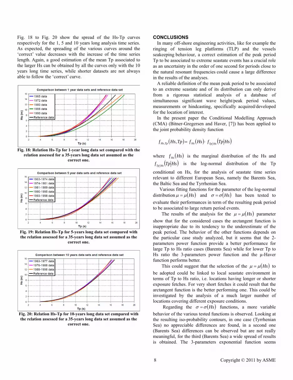
Fig. 18 to Fig. 20 show the spread of the Hs-Tp curves respectively for the 1, 5 and 10 years long analysis time series. As expected, the spreading of the various curves around the ‘correct’ value decreases with the increase of the time series length. Again, a good estimation of the mean Tp associated to the larger Hs can be obtained by all the curves only with the 10 years long time series, while shorter datasets are not always able to follow the ‘correct’ curve.

Fig. 18: Relation Hs-Tp for 1-year long data set compared with the

relation assessed for a 35-years long data set assumed as the correct one.

Fig. 19: Relation Hs-Tp for 5-years long data set compared with the relation assessed for a 35-years long data set assumed as the

correct one.

Fig. 20: Relation Hs-Tp for 10-years long data set compared with the relation assessed for a 35-years long data set assumed as the

correct one.

CONCLUSIONS In many off-shore engineering activities, like for example the

ringing of tension leg platforms (TLP) and the vessels seakeeping behaviour, a correct estimation of the peak period Tp to be associated to extreme seastate events has a crucial role as an uncertainty in the order of one second for periods close to the natural resonant frequencies could cause a large difference in the results of the analyses.

A reliable definition of the mean peak period to be associated to an extreme seastate and of its distribution can only derive from a rigorous statistical analysis of a database of simultaneous significant wave height/peak period values, measurements or hindcasting, specifically acquired/developed for the location of interest.

In the present paper the Conditional Modelling Approach (CMA) (Bitner-Gregersen and Haver, [7]) has been applied to the joint probability density function

( ) ( ) ( )HsTpfHsfTpHsf HsTpHsTpHs ⋅=,,

where ( )Hsf Hs is the marginal distribution of the Hs and

( )HsTpf HsTp is the log-normal distribution of the Tp

conditional on Hs, for the analysis of seastate time series relevant to different European Seas, namely the Barents Sea, the Baltic Sea and the Tyrrhenian Sea.

Various fitting functions for the parameter of the log-normal distribution ( )Hsμμ = and ( )Hsσσ = has been tested to evaluate their performances in term of the resulting peak period to be associated to large return period events.

The results of the analysis for the ( )Hsμμ = parameter show that for the considered cases the arctangent function is inappropriate due to its tendency to the underestimate of the peak period. The behavior of the other functions depends on the particular case study analyzed, but it seems that the 2-parameters power function provide a better performance for large Tp to Hs ratio cases (Barents Sea) while for lower Tp to Hs ratio the 3-parameters power function and the μ-Haver function performs better.

This could suggest that the selection of the ( )Hsμμ = to be adopted could be linked to local seastate environment in terms of Tp to Hs ratio, i.e. locations having longer or shorter exposure fetches. For very short fetches it could result that the arctangent function is the better performing one. This could be investigated by the analysis of a much larger number of locations covering different exposure conditions.

Regarding the (Hs)σσ = functions, a more variable behavior of the various tested functions is observed. Looking at the resulting iso-probability contours, in one case (Tyrrhenian Sea) no appreciable differences are found, in a second one (Barents Sea) differences can be observed but are not really meaningful, for the third (Barents Sea) a wide spread of results is obtained. The 3-parameters exponential function seems

8 Copyright © 2011 by ASME

clearly to overestimate on respect to the dataset points. The 2-parameters exponential and the σ-Haver functions provide different results but it is hardly definable which one is better performing, the 2-parametrs exponential apparently being more close to the dataset points but possibly providing a too narrow range of Tp values. σ-Haver function could be a good compromise, being conservative and not too wide on respect to the dataset points.

A more general assessment about the absolute performance of the various functions needs the treatment of a much more large number of cases for different metocean conditions. This was beyond the scope of the paper, but the analyses performed suggest that it is recommendable to test various fitting functions both for ( )Hsμμ = and ( )Hsσσ = by comparison with the available dataset points in order to select the better performing ones.

A last outcome of the present paper concerns the minimum length of the time series to be used for a reliable estimation of the Hs/Tp relation. In fact, repeated tests on different time series of equal length, if such length was not sufficiently long, showed a rather wide spread of results in term of Tp associated to large return period Hs. Increasing the length of the time series the spread of the results around the supposed right values decreases.

For the present considered case (Barents Sea), it seems that using 1 year long time series significant errors larger than 1 second could occur already for 1 year return period events. For 5 years long time series the error is reduced especially for 1 and 10 years return period, but errors in the order of 1 second could occur for 100 years return period. Therefore, for a reliable estimation of the peak period Tp to be associated to extreme seastates it would be recommendable to use an at least 10 years long time series.

REFERENCES [1] Faltinsen, O. M., 1993, Sea Loads on Ships and Offshore Structures, Cambridge University Press, Cambridge, UK. [2] DNV Recommended Practice DNV-RP-C205, 2007, “Environmental Conditions and Environmental Loads”, DNV, Norway. [3] Carter, D., J., T., Challenor, P., G., Ewing, J., A., Pitt, E., G., Srokosz, M. A. Tucker, M., J., 1986, Estimating Wave Climate Parameters for Engineering Applications, Department of Energy, Offshore Technology Report OTH 86 228, Her Majesty’s Stationery Office, London, UK. [4] Bretschneider, C. L. (1952), “The generation and decay of wind waves in deep water”, Trans. A.G.U., 33(3), 381–389. [5] CERC, 1984, “Shore Protection Manual”, US Army, Coastal Engineering Research Center, US.

[6] Prince-Wright, R., 1995, ”Maximum Likelihood Models of Joint Environmental Data for TLP Design”, Proc.OMAE 1995 Conference, Copenhagen, Denmark, Vol. 2. [7] Bitner-Gregersen, E. M., and Haver, S., 1991, ”Joint Environmental Model for Reliability Calculations”, Proc.ISOPE 1991 Conference, Edinburgh, UK, Vol. 1, pp. 246-253. [8] Haver, S., 1980, ”Analysis of Uncertainties Related to the Stochastic Modelling of Ocean Waves”. Department of Marine Technology – The Norwegian Institute of Technology – University of Trondheim. Report UR-80-09. [9] Haver, S. and Nyhus, H., A., 1986, ”A Wave Climate Description for Long Term Response Calculations”, Proc. Int. OMAE 1986 Symposium, Tokyo, Japan, Vol. IV, pp. 27-34. [10] Bitner-Gregersen, E. M., 2005, ”Joint Probabilistic Description for Combined Seas”, Proc.OMAE 2005 Conference, Halkidiki, Greece. [11] Oceanweather, NEXT-RA project, http://www.oceanweather.com/metocean/next/index.html

[12] Danish Hydraulic Institute, BALSEA project, http://www.dhigroup.com/Solutions/MarineInfrastructureAndEnergy/MetoceanData.aspx [13] Istituto Superiore per la Protezione e la Ricerca Ambientale (ISPRA), Rete Ondametrica Nazionale (RON), http://www.telemisura.it/

[14] Haver, S., 1985, ”Wave Climate Off Northern Norway”. J. Applied Ocean Research, Vol. 7 No. 2, pp. 85-92.

[15] Jonathan, P., Flynn, J., Ewans, K., 2010, ”Joint Modelling of Wave Spectra Parameters for Extreme Seastates”. J. Ocean Engineering, Vol. 37, pp. 1070-1080.

9 Copyright © 2011 by ASME