Convergence of Estimators in LLS Analysis

arX

iv:m

ath/

0508

297v

2 [

mat

h.ST

] 3

Oct

200

5

CONVERGENCE OF ESTIMATORS IN LLS ANALYSIS

MIKHAIL KOVTUN, ANATOLIY YASHIN, AND IGOR AKUSHEVICH

Abstract. We establish necessary and sufficient conditions for consistency ofestimators of mixing distribution in linear latent structure analysis.

1. Introduction

Linear latent structure (LLS) analysis is aimed to derive properties of populationas whole and properties of individuals from a large number of categorical measure-ments made on each individual in a sample. An exposition of LLS analysis is givenin Kovtun et al. (2005b).

LLS analysis searches for representation of the observed joint distribution ofrandom variables (representing measurements) as a mixture of independent distri-butions, i.e. distributions, in which random variables are mutually independent.Such approach is common for all branches of latent structure analysis. The specificLLS assumption is that the mixing distribution is supported by a low-dimensionallinear subspace of the space of independent distributions.

When dimensionality of the supporting subspace is sufficiently smaller than thenumber of random variables and under some regularity conditions, a set of low-order moments (of order up to number of measurements) of mixing distributionis identifiable. Increasing the size of the sample does not increase the number ofidentifiable moments—only precision of their estimates increases. Thus, the mixingdistribution in LLS analysis is only partially identifiable. In Kovtun et al. (2005b)we suggested an estimator of the mixing distribution. This estimator, however,does not converge to the true mixing distribution when the sample size tends toinfinity. The natural question arise: what is the value of such partially identifiablemodel and in what sense the suggested estimator is useful?

In this article, we give one possible answer to this question. Assume that one hasan infinite sequence of possible measurements; a particular survey uses finite numberof measurements from this sequence. Then a sequence of estimates of mixing distri-bution obtained in a sequence of surveys with increasing number of measurementsconverges to the true mixing distribution. The necessary and sufficient conditionfor this convergence is pairwise orthogonality of independent distributions beingmixed.

2000 Mathematics Subject Classification. Primary 62G05; Secondary 60E99.Key words and phrases. Latent structure analysis, mixed distributions, convergence of esti-

mators, orthogonality of measures, weak convergence, tail σ-algebra, law of large numbers.The work of the first author was supported by the Office of Vice Provost for Research, Duke

University.The work of the second author was supported by NIH/NIA grants PO1 AG08761-01, U01

AG023712 and U01 AG07198.The work of the third author was supported by NIH/NIA grant P01 AG17937-05.

1

http://arXiv.org/abs/math/0508297v2

2 MIKHAIL KOVTUN, ANATOLIY YASHIN, AND IGOR AKUSHEVICH

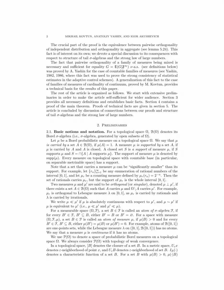
The crucial part of the proof is the equivalence between pairwise orthogonalityof independent distribution and orthogonality in aggregate (see lemma 5.24). Thisfact is of interest on its own; we devote a special discussion to its consequences withrespect to structure of tail σ-algebras and the strong law of large numbers.

The fact that pairwise orthogonality of a family of measures being mixed isnecessary and sufficient for equality G = E(G|F∞) ν-a.s. (see definitions below)was proved by A. Yashin for the case of countable families of measures (see Yashin,1982, 1986, where this fact was used to prove the strong consistency of statisticalestimates in the adaptive control schemes). A generalization of this fact to the caseof families of measures of cardinality of continuum, proved by M. Kovtun, providesa technical basis for the results of this paper.

The rest of the article is organized as follows. We start with extensive prelim-inaries in order to make the article self-sufficient for wider audience. Section 3provides all necessary definitions and establishes basic facts. Section 4 contains aproof of the main theorem. Proofs of technical facts are given in section 5. Thearticle is concluded by discussion of connections between our proofs and structureof tail σ-algebras and the strong law of large numbers.

2. Preliminaries

2.1. Basic notions and notation. For a topological space Ω, B(Ω) denotes itsBorel σ-algebra (i.e., σ-algebra, generated by open subsets of Ω).

Let µ be a Borel probabilistic measure on a topological space Ω. We say that µis carried by a set A ∈ B(Ω), if µ(A) = 1. A measure µ is supported by a set A, ifµ is carried by A and A is closed. A closed set S is a support of measure µ, if Ssupports µ and S = ∩A | A supports µ. The support of measure µ is denoted bysupp(µ). Every measure on topological space with countable base (in particular,on separable metrizable space) has a support.

Note that a set that carries a measure µ can be “significantly smaller” than itssupport. For example, let rn∞n=1 be any enumeration of rational numbers of theinterval [0, 1], and let µr be a counting measure defined by µr(rn) = 2−n. Then theset of rationals carries µr, but the support of µr is the whole interval [0, 1].

Two measures µ and µ′ are said to be orthogonal (or singular), denoted µ ⊥ µ′, ifthere exists a set A ∈ B(Ω) such that A carries µ and Ω\A carries µ′. For example,µr is orthogonal to Lebesgue measure λ on [0, 1], as µr is carried by rationals andλ is carried by irrationals.

We write µ ≪ µ′ if µ is absolutely continuous with respect to µ′, and µ ∼ µ′ ifµ is equivalent to µ′ (i.e., µ≪ µ′ and µ′ ≪ µ).

For a measurable space (Ω,F), a set B ∈ F is called an atom of σ-algebra F, iffor every B′ ∈ F, B′ ⊆ B, either B′ = B or B′ = ∅. For a space with measure(Ω,F, µ), a set B ∈ F is called an atom of measure µ, if µ(B) > 0 and for everyB′ ∈ F, B′ ⊆ B, either µ(B′) = µ(B) or µ(B′) = 0. For example, atoms of B([0, 1])are one-points sets, while the Lebesgue measure λ on ([0, 1],B([0, 1])) has no atoms.We say that a measure µ is continuous if it has no atoms.

We use P(Ω) to denote a space of probabilistic Borel measures on a topologicalspace Ω. We always consider P(Ω) with topology of weak convergence.

In a topological space, [B] denotes the closure of a set B. In a metric space, Uεxdenotes ε-neighborhood of point x, and UεB denotes ε-neighborhood of set B. IB(·)denotes a characteristic function of a set B. For a set B with µ(B) > 0, µ(·|B)

CONVERGENCE OF ESTIMATORS IN LLS ANALYSIS 3

denotes a probabilistic measure conditional on B (i.e., µ(·|B)(B′) = µ(B′|B) =µ(B′∩B)/µ(B)). Bn ↓ B abbreviates the statement “B1 ⊇ B2 ⊇ . . . and

⋂nBn =

B.” Bn B abbreviates the statement “Bn ↓ B and ∀ ε > 0 ∃m ∀n > m : Bn ⊆UεB.” δx denotes a measure concentrated at a single point x.

We shall use the following properties of Borel measures on a metric spaces:

(1) x ∈ supp(µ) ⇔ ∀ε > 0 : µ(Uεx) > 0(2) For every x ∈ supp(µ) there exists a sequence of sets Bnn such that

µ(Bn) > 0 and Bn x(3) µ′ ≪ µ ⇒ supp(µ′) ⊆ supp(µ)(4) If µ(B) > 0, then µ(·|B) ≪ µ and supp(µ(·|B)) ⊆ supp(µ)

(5) If Bn x and µn is carried by Bn, then µnw−→ δx

2.2. Lebesgue spaces. The notion of Lebesgue space was introduced and its mainproperties were established in Rokhlin (1949) (English translation—Rohlin (1952)).

Let (Ω,F, µ) be a space with measure. In this subsection, all spaces with measureare assumed to be complete, i.e. B ∈ F, µ(B) = 0, and B′ ⊆ B imply B′ ∈ F. Wealso assume that µ(Ω) = 1.

A countable system of measurable sets G = Γi∞i=1 is called a basis of (Ω,F, µ),if it possesses the following two properties:

(L) ∀B ∈ F ∃C ∈ σ(G) : B ⊆ C ∧ µ(B) = µ(C)(M) ∀ω 6= ω′ ∈ Ω ∃ i : (ω ∈ Γi ∧ ω′ 6∈ Γi) ∨ (ω′ ∈ Γi ∧ ω 6∈ Γi)

A space with measure is called separable, if it has a basis.If Ω is a second-countable T0 topological space (in particular, if Ω is a separa-

ble metric space) and µ is a measure defined on its Borel σ-algebra B(Ω), then(Ω,Bµ(Ω), µ), where Bµ(Ω) is Lebesgue completion of Borel σ-algebra with respectto measure µ and µ is continuation of µ onto Bµ(Ω), is a separable space withmeasure, and topology base serves as a basis in the above sense.

Let (Ω,F, µ) be a separable space with measure, and let G = Γii be its basis.Consider intersections

(1)∞⋂

i=1

Υi, where either Υi = Γi or Υi = Ω \ Γi

Due to property (M), every such intersection cannot contain more than onepoint. Furthermore, every one-point set is representable in form (1) (to obtain aset consisting of ω, take Υi = Γi if ω ∈ Γi, and Υi = Ω \ Γi otherwise).

A separable space with measure (Ω,F, µ) is said to be complete with respect tobasis G = Γii, if every intersection (1) is nonempty (and thus, consists of onepoint). A separable space with measure (Ω,F, µ) is said to be complete (mod 0)with respect to basis G = Γii, if it is isomorphic (mod 0) to a space with mea-sure (Ω′,F′, µ′), which is complete with respect to its basis G′ = Γ′

ii, and thisisomorphism transforms base G to basis G′.

Important fact is (Rokhlin, 1949; Rohlin, 1952, §2, n2): if a separable spacewith measure is complete (mod 0) with respect to some basis, then it is complete(mod 0) with respect to every other basis.

A separable space with measure is called Lebesgue space, if it is complete (mod 0)with respect to its bases.

It happens that many important spaces with measures are Lebesgue spaces. Inparticular, if Ω is a separable (in topological sense) complete metric space and µ

https://www.researchgate.net/publication/247040054_On_the_fundamental_ideas_of_measure_theory?el=1_x_8&enrichId=rgreq-cacecd54-2402-40ca-98f4-163fb30376b1&enrichSource=Y292ZXJQYWdlOzIxMjE2NzU7QVM6OTkwNzg2NDYwMDk4NzRAMTQwMDYzMzU5ODg3MQ==


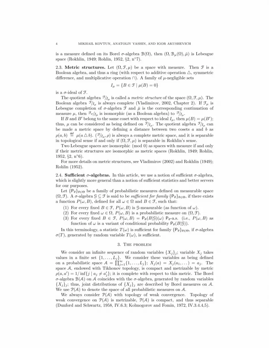
is a measure defined on its Borel σ-algebra B(Ω), then (Ω,Bµ(Ω), µ) is Lebesguespace (Rokhlin, 1949; Rohlin, 1952, §2, n7).

2.3. Metric structures. Let (Ω,F, µ) be a space with measure. Then F is aBoolean algebra, and thus a ring (with respect to additive operation , symmetricdifference, and multiplicative operation ∩). A family of µ-negligible sets

Iµ = B ∈ F | µ(B) = 0is a σ-ideal of F.

The quotient algebra F/Iµis called a metric structure of the space (Ω,F, µ). The

Boolean algebra F/Iµis always complete (Vladimirov, 2002, Chapter 2). If Fµ is

Lebesgue completion of σ-algebra F and µ is the corresponding continuation ofmeasure µ, then Fµ/Iµ

is isomorphic (as a Boolean algebra) to F/Iµ.

If B and B′ belong to the same coset with respect to ideal Iµ, then µ(B) = µ(B′);thus, µ can be considered as being defined on F/Iµ

. The quotient algebra F/Iµcan

be made a metric space by defining a distance between two cosets a and b as

ρ(a, b)def

= µ(a b). (F/Iµ, ρ) is always a complete metric space, and it is separable

in topological sense if and only if (Ω,F, µ) is separable in Rokhlin’s sense.Two Lebesgue spaces are isomorphic (mod 0) as spaces with measure if and only

if their metric structures are isomorphic as metric spaces (Rokhlin, 1949; Rohlin,1952, §2, n6).

For more details on metric structures, see Vladimirov (2002) and Rokhlin (1949);Rohlin (1952).

2.4. Sufficient σ-algebras. In this article, we use a notion of sufficient σ-algebra,which is slightly more general than a notion of sufficient statistics and better serversfor our purposes.

Let Pθθ∈Θ be a family of probabilistic measures defined on measurable space(Ω,F). A σ-algebra G ⊆ F is said to be sufficient for family Pθθ∈Θ, if there existsa function P (ω,B), defined for all ω ∈ Ω and B ∈ F, such that:

(1) For every fixed B ∈ F, P (ω,B) is G-measurable (as function of ω).(2) For every fixed ω ∈ Ω, P (ω,B) is a probabilistic measure on (Ω,F).(3) For every fixed B ∈ F, P (ω,B) = Pθ(B|G)(ω) Pθ-a.s. (i.e., P (ω,B) as

function of ω is a variant of conditional probability Pθ(B|G)).

In this terminology, a statistic T (ω) is sufficient for family Pθθ∈Θ, if σ-algebraσ(T ), generated by random variable T (ω), is sufficient.

3. The problem

We consider an infinite sequence of random variables Xjj; variable Xj takesvalues in a finite set 1, . . . , Lj. We consider these variables as being definedon a probabilistic space A =

∏∞j=11, . . . , Lj; Xj(a) = Xj(a1, . . . ) = aj . The

space A, endowed with Tikhonov topology, is compact and metrizable by metricρ(a, a′) = 1/ infj | aj 6= a′j; it is complete with respect to this metric. The Borelσ-algebra B(A) on A coincides with the σ-algebra, generated by random variablesXjj; thus, joint distributions of Xjj are described by Borel measures on A.We use P(A) to denote the space of all probabilistic measures on A.

We always consider P(A) with topology of weak convergence. Topology ofweak convergence on P(A) is metrizable, P(A) is compact, and thus separable(Dunford and Schwartz, 1958, IV.6.3; Kolmogorov and Fomin, 1972, IV.3.4.4,5).


Among all joint distributions of Xjj, we distinguish independent ones, i.e.those distributions, in which random variables Xjj are mutually independent. Tospecify an independent distribution, one needs to specify only probabilities βjl =P(Xj = l). Then, due to independence, one has for cylinders P(Xj1 = l1 ∧ · · · ∧Xjp

= lp) = βj1l1 · · ·βjplp , and as cylinders compose a topology base, this uniquelyextends to B(A). Thus, any independent distribution is uniquely described by aninfinite-dimensional vector β = (β11, . . . , β1L1 , . . . , βj1, . . . , βjLj

, . . . ). To specify adistribution, such vector must satisfy conditions:

(2)

0 ≤ βjl ≤ 1 for all j and l∑Lj

l=1 βjl = 1 for all j

The set of vectors satisfying (2) is a convex infinite-dimensional body P in R∞.Let Pβ denote the independent distribution over A corresponding to a vector β ∈ P .

Our goal is to investigate a class of mixtures of independent distributions, i.e.those distributions P on A which can be represented in form:

(3) P(A) =

∫

P

Pβ(A)µ(dβ) for all A ∈ B(A)

where µ is a probabilistic measure on P . For this definition of mixture to becorrect, one needs to show that the mapping β 7→ Pβ(A) is measurable for everyBorel A ⊆ A. We show a stronger fact:

Proposition 3.1. The mapping β 7→ Pβ is continuous with respect to Tikhonovtopology on R∞ and topology of weak convergence on P(A).

Proof. It is sufficient to show that for every converging sequence βn → β in P , thesequence Pβn weakly converges and limPβn = Pβ . For this, in turn, one needs toshow that Pβn(C) → Pβ(C) for every cylinder C with Pβ(∂C) = 0 (Shiryaev, 2004,III.1.5). In A every cylinder is open-closed set; thus, this must be shown for allcylinders. But for a cylinder C with base aj1 , . . . , ajp

one has Pβn(C) =∏

q βnjqajq

,

and required convergence follows directly from the convergence βn → β.

Corollary 3.2. For every A ∈ B(A), the mapping β 7→ Pβ(A) is measurable (w.r.t.corresponding Borel σ-algebras).

Proof. By Dellacherie and Meyer (1978, III.55,60), the mapping P 7→ P(B) is mea-surable. Thus, our mapping is measurable as a composition of two measurablemappings.

We abbreviate the equation (3) to P = Mix(µ). We also use Pµ to denote Mix(µ).One of the questions that we are interested in is conditions for identifiability of

mixtures of independent distributions (in sense of Teicher, 1960), i.e. under whatconditions the mixture Mix(µ) uniquely defines the mixing measure µ. It is easy toshow, however, that without additional restrictions any distribution on A can berepresented as a mixture of independent ones, and (except degenerate cases) everydistribution has infinitely many such representations.

For a distribution µ on P , let L(µ) denote the smallest linear subspace of R∞

supporting µ (this subspace is a linear span of supp(µ)). We say that a mixingdistribution µ has rank K, rank(µ) = K, if dim(L(µ)) = K. We say that adistribution P ∈ P(A) has rank not greater than K, rank(P) ≤ K, if P = Mix(µ)

https://www.researchgate.net/publication/229680035_Mixture_Distributions-I?el=1_x_8&enrichId=rgreq-cacecd54-2402-40ca-98f4-163fb30376b1&enrichSource=Y292ZXJQYWdlOzIxMjE2NzU7QVM6OTkwNzg2NDYwMDk4NzRAMTQwMDYzMzU5ODg3MQ==


for some measure µ with rank(µ) = K; further, rank(P) = K, if rank(P) ≤ K andrank(P) K − 1.

The question of identifiability can be now splitted into two subquestions:

• For a distribution of rank K, what are conditions for identifiability of aK-dimensional linear subspace carrying a mixing measure? More precisely:what are conditions for implication

rank(P) = KP = Mix(µ) = Mix(µ′)rank(µ) = rank(µ′) = K

⇒ L(µ) = L(µ′)

to be true?• For a fixed K-dimensional subspace L of R∞, what are conditions for iden-

tifiability of mixing measure carried by this subspace? More precisely: whatare conditions for implication

Mix(µ) = Mix(µ′)L(µ) = L(µ′) = L

⇒ µ = µ′

to be true?

We shall address these questions full detail in another article. Here, we men-tion a sufficient condition of identifiability established (in slightly different form)in Kovtun et al. (2005b). Let C = (Covµ(βjl, βj′l′))jl,j′l′ be (infinite) covariance

matrix of the mixing measure µ. Suppose that all minors of C of size K + 1 aredegenerate and all minors of size K are non-degenerate. Then rank(µ) = K andany mixing measure of rank not greater than K, which produces the same mixture,coincides with µ.

When the mixing measure is identifiable, the question arise how the mixingmeasure can be estimated. The main topic of the present article is the investiga-tion of properties of the estimator, outlined in Kovtun et al. (2005b). The formaldescription of this estimator is given below.

Let us fix a K-dimensional subspace L of R∞ such that P0 = P ∩L is a (K−1)-dimensional body. Let us also fix λ1, . . . , λK , a set of K linearly independentvectors from P0. Then every vector β ∈ P0 can be uniquely represented in formβ =

∑k gkλ

k, and∑

k gk = 1. Thus, we have a linear isomorphism β : Q → P0,where Q is a (K−1)-dimensional body in RK , belonging to the hyperplane

∑k gk =

1. For brevity, we write Pg instead of Pβ(g).Because the mapping β : Q→ P0 is obviously continuous, we immediately obtain

from proposition 3.1:

Proposition 3.3. The mapping g 7→ Pg is continuous with respect to standardEuclidean topology on Q and topology of weak convergence on P(A).

Proposition 3.4. For every B ∈ B(A), the mapping g 7→ Pg(B) is measurable(w.r.t. corresponding Borel σ-algebras).

Due to the isomorphism β : Q → P0, every measure µP0 on P0 induces measureµQ on Q (by letting µQ(B) = µP0(β(B))) and vice versa. We usually drop the indexand write just µ, as it is obvious from the context what measure is considered.

Thus, every probabilistic measure µ on Q generates a probabilistic measure Pµ

by means of (3).Now we develop a slightly different view on the problem. Measure µ may be

considered as a distribution of random variable G that takes values in Q. Random


variables G,X1, . . . may be considered as defined on a common probabilistic spaceΩ = Q× A; G(g, a1, . . . ) = g and Xj(g, a1, . . . ) = aj .

A distribution µ of G induces a joint distribution ν of G,X1, . . . : for Borel setsB ∈ B(Q) and A ∈ B(A),

(4) ν(B ×A) =

∫

B

Pg(A)µ(dg)

When A is a cylinder with base aj1 , . . . , ajp, one obtains

ν(B ×A) =

∫

B

p∏

q=1

K∑

k=1

gkλkjqajq

µ(dg)

By the Kolmogorov’s theorem, the measure ν uniquely extends from sets of formB × C to the Borel σ-algebra of Ω.

The marginal distribution of ν on A is Pµ, and the marginal distribution of ν onQ is µ. Note that ν is not a product of µ and Pµ.

Let Fn = σ(X1, . . . , Xn), an increasing sequence of σ-subalgebras of B(Ω), andlet F∞ = σ(X1, . . . ) = σ(

⋃n Fn). Consider conditional expectations E(G | Fn) and

E(G | F∞). By Levi theorem, E(G | Fn) → E(G | F∞), ν-a.s. and in the sense ofL1.

On the other hand, every element of Fn and F∞ has a form Q× A, A ∈ B(A)(in other words, sets Q× a are atomic w.r.t. σ-algebras Fn, F∞). Thus, valuesE(G | Fn)(g, a), E(G | F∞)(g, a) do not depend on g. This allows us to definefunctions en : A → Q, e∞ : A → Q by letting en(a) = E(G | Fn)(g, a) and similarlyfor e∞. Again, en → e∞ Pµ-a.s. and in the sense of L1.

Functions en, e∞ transform measure Pµ on A to measures µn, µ∞ on Q byletting µn(B) = Pµ(e−1

n (B)) for every B ∈ B(Q), and similarly for µ∞. Simple,but important fact is:

Proposition 3.5. The sequence µnn weakly converges to µ∞.

Proof. It is sufficient to show (Shiryaev, 2004, III.1.3.V) that∫φ(g) µn(dg) con-

verges to∫φ(g) µ∞(dg) for every uniformly continuous function φ : Q → R. By

changing variables, one obtains∫φ(g) µn(dg) =

∫φ(en(a))Pµ(da)

∫φ(g) µ∞(dg) =

∫φ(e∞(a))Pµ(da)

and required convergence is equivalent to φ enL1

−−→ φ e∞, which follows from the

convergence enL1

−−→ e∞ due to the uniform continuity of φ.

Functions en do not depend on “tails” of their arguments: if aj = a′j for j =1, . . . , n, then en(a) = en(a′). This allows to construct µn only from knowledgeof distribution of X1, . . . , Xn and from en. One possible way to estimate en wasestablished in Kovtun et al. (2005a,b); Kovtun et al. (2005b) suggested to use µn

as an estimator of µ. Conditions for consistency of this estimator are the maintopic of the present article.

Note that ν, en, µn, etc. depend on the mixing measure µ. To stress suchdependency, we use sometime notation ν[µ], en[µ], µn[µ], etc. We shall drop [µ]whenever the mixing measure µ is obvious from the context.


We shall also use σ-algebras F∞n = σ(Xn, Xn+1, . . . ) and the tail σ-algebra

X =⋂

n F∞n . These σ-algebras are considered as algebras of subsets of either A

or Ω = Q× A (in the latest case, they consist of cylinders built on subsets of A).It should be always clear from the context what case is considered.

4. Main theorem

The main theorem, proved in this section, establishes necessary and sufficient

conditions for convergence µnw−→ µ. It is formulated as nine equivalent conditions,

which are naturally splitted into three groups. The first group consists of conditions(1) and (2); they are just statements of convergence. The second group consists ofconditions (3), (4), (5), and (6); these conditions are expressed in terms of randomvariable G and related entities. The last group consists of conditions (7), (8),and (9). Condition (7) is just statement of pairwise orthogonality of independentmeasures being mixed, while other two are criteria of orthogonality in terms ofHellinger integrals.

The condition (4), G = E(G | F∞) ν-a.s., looks surprising for the first glance: Gas function of ω = (g, a) does not depend on a, while E(G | F∞) does not dependon g. The only points where these two functions coincide is the graph of functione∞. But, according to condition (3), this graph has ν-measure 1, and thus equalityholds ν-a.s.

This condition has an important consequence: if the sequence of outcomesa = (a1, . . . ) is generated by an independent distribution Pg, then e∞(a) withprobability 1 gives this distribution. This fact justifies usage of conditional expec-tation E(G | X1 = a1, . . . , Xj = aj) as estimation of individual position in phasespace Q, suggested in Kovtun et al. (2005b).

Theorem 4.1. The following conditions are equivalent:

(1) For every µ ∈ P(Q), µn[µ]w−→ µ

(2) For every µ ∈ P(Q), µ∞[µ] = µ(3) For every µ ∈ P(Q), ν[µ](Γe∞[µ]) = 1 (where Γf denotes the graph of a

function f)(4) For every µ ∈ P(Q), G = E(G | F∞) ν[µ]-a.s.(5) For every µ ∈ P(Q), there exists a variant of regular conditional distribution

of G with respect to F∞ (i.e., a function P (ω,B), ω ∈ Ω, B ∈ B(Q)) suchthat for every ω ∈ Ω, the distribution P (ω, ·) is concentrated at a singlepoint.

(6) For every µ ∈ P(Q), there exists a set Q1 ⊆ Q with µ(Q1) = 1 such thattail σ-algebra X is sufficient for the family of measures Pg | g ∈ Q1.

(7) ∀g′, g′′ ∈ Q : g′ 6= g′′ ⇒ Pg′ ⊥ Pg′′

(8) ∀g′, g′′ ∈ Q : g′ 6= g′′ ⇒ ∏∞j=1

∑Lj

l=1

√βjl(g′)βjl(g′′) = 0

(9) ∀g′, g′′ ∈ Q : g′ 6= g′′ ⇒ ∑∞j=1

∑Lj

l=1

(√βjl(g′) −

√βjl(g′′)

)2

= ∞

Proof. In order to make the proof of main theorem more clear, we moved proofs ofall technical facts to the next section.

(1) ⇔ (2). Follows from the proposition 3.5.

(2) ⇒ (7). Take arbitrary g′, g′′ ∈ Q and take µ ∈ P(Q) being concentrated atpoints g′, g′′ with weights α and 1−α, where 0 < α < 1. Then for every B ∈ B(Q),


µ(B) = µ∞(B) = Pµ(e−1∞ (B)). In particular, for A′ = e−1

∞ (g′), one obtainsPµ(A′) = µ(g′) = α.

Further, one obtains:

g′ · α = g′ ·∫

A′

Pµ(da) =

∫

A′

g′ Pµ(da) =

∫

A′

e∞(a)Pµ(da) =

∫

Q×A′

E(G | F∞)(ω) ν(dω) =

∫

Q×A′

G(ω) ν(dω)(*)=

g′ · ν(g′ ×A′) + g′′ · ν(g′′ ×A′)(**)= g′ · αPg′(A′) + g′′ · (1 − α)Pg′′ (A′)

(equality (*) holds as G(ω) is a simple function, taking with non-zero probabilityonly values g′ and g′′; equality (**) follows from definition of ν, equation (4)).

As g′ and g′′ are linearly independent vectors, the above equation implies thatPg′(A′) = 1 and Pg′′ (A′) = 0, which means Pg′ ⊥ Pg′′ , q.e.d.

(7) ⇔ (6). Follows from lemmas 5.27 and 5.28.

(7) ⇒ (5). We shall show a stronger fact, that there exists a variant of regularconditional distribution with respect to the tail σ-algebra X, which has the requiredproperty and which serves as regular conditional distribution w.r.t. F∞ as well.Take P ((g, a), B) = δϕ(a)(B), where ϕ defined by lemma 5.25. For every ω = (g, a),P (ω,B) is, by definition, a probabilistic measure on (Q,B(Q)), and this measureis concentrated at a single point. Thus, one has to show that for every B ∈ B(Q),ν(G−1(B)|X)(ω) = E(IG−1(B)|X)(ω) = P (ω,B) ν-a.s. As by lemma 5.25 P (ω,B)is X-measurable, one needs to show that for every Q×A ∈ X

(5)

∫

Q×A

IG−1(B)(ω) ν(dω) =

∫

Q×A

P (ω,B) ν(dω)

Using Robbins’ theorem (section 5.4), the left-hand side is reduced to:

∫

Q×A

IG−1(B)(ω) ν(dω) =

∫

Q×A

IB(g) ν(dω) =

∫

Q

(∫

A

IB(g)Pg(da)

)µ(dg) =

∫

Q

IB(g)

(∫

A

IA(a)Pg(da)

)µ(dg) =

∫

Q

IB(g)Pg(A)µ(dg)

where h is a homomorphism defined in section 5.4. The right-hand side, in turn, isreduced to:∫

Q×A

P (ω,B) ν(dω) =

∫

Q×A

δϕ(a)(B) ν(dω) =

∫

Q

(∫

A

δϕ(a)(B)Pg(da)

)µ(dg) =

∫

Q

δg(B)Pg(A)µ(dg) =

∫

Q

IB(g)Pg(A)µ(dg)

which proves the equality (5). Finally, note that the proof of the equality (5)remain valid, if A is taken from F∞. Thus, P (ω,B) is also a regular conditionaldistribution w.r.t. F∞.


(5) ⇒ (4). Let P (ω,B) be a regular conditional distribution of G w.r.t. F∞, suchthat for every ω the distribution P (ω, ·) is concentrated at a single point. Note thatP (ω,B) as function of ω = (g, a) does not depend on g (as F∞ consists of cylindersQ × A); this allows us to write P (a,B). Let further g(a) be the point, whichthe distribution P (a, ·) is concentrated at. By Shiryaev (2004, II.7.7), conditionalexpectation can be calculated using regular conditional distribution:

E(G|F∞)(g′, a′) =

∫

Q

gP (a′, dg) = g(a′)

For arbitrary C ∈ B(Ω) one has ν(C) =∫

AP (a, Ca)Pµ(da), where Ca = g |

(g, a) ∈ C. Applying this formula to C0 = ω | G(ω) = E(G|X)(ω) = (g, a) |g = g(a) one obtains

ν(C0) =

∫

A

P (a, g(a))Pµ(da) =

∫

A

1 · Pµ(da) = 1

which proves that G(ω) = E(G|X)(ω) ν-a.s.

(4) ⇒ (3). Follows from:

Γe∞ = (g, a) | g = e∞(a) = (g, a) | G(g, a) = E(G|X)(g, a)

(3) ⇒ (2). First, note that for every B ∈ B(Q) one has (B × A) ∩ Γe∞ =(Q × e−1

∞ (B)) ∩ Γe∞. Then (as P(A) = 1 ⇒ P(B) = P(B ∩ A) and µ andPµ are marginals of ν) one obtains µ(B) = ν(B × A) = ν((B × A) ∩ Γe∞) andµ∞(B) = Pµ(e−1

∞ (B)) = ν(Q × e−1∞ (B)) = ν((Q × e−1

∞ (B)) ∩ Γe∞), which givesµ(B) = µ∞(B) for every Borel B, q.e.d.

(7) ⇔ (8). By Shiryaev (2004, III.9.3, theorem 3), Pg′ ⊥ Pg′′ is equivalent toH(Pg′ ,Pg′′) = 0, where H(P,P′) is a Hellinger integral of order 1

2 . When randomvariables X1, . . . are independent (which is the case for distributions Pg′ and Pg′′),their joint distribution is the product of individual distributions, and Hellingerintegral for the joint distributions is the product of Hellinger integrals for the indi-vidual distributions (Shiryaev, 2004, III.9.2). The direct computation (see section

5.1) gives H(Pg′ ,Pg′′ ) =∏∞

j=1

∑Lj

l=1

√βjl(g′)βjl(g′′), q.e.d.

(8) ⇔ (9). Follows from lemma 5.9.

5. Auxilary lemmas

5.1. Hellinger integrals and related series. Let Pjg denote the distribution of

Xj that corresponds to g. Pjg is defined on a finite probabilistic space 1, . . . , Lj,

and is fully determined by vector (βj1(g), . . . , βjLj(g)). The Hellinger integral of

order 12 (see Shiryaev, 2004, III.9.3) for P

jg′ and P

jg′′ is:

(6) H(Pjg′ ,P

jg′′ ) =

Lj∑

l=1

√βjl(g′)βjl(g′′)

As random variables Xjj are mutually independent in distribution Pg, themeasure Pg is a product of measures P

jg; thus, the Hellinger integral for distributions

Pg′ and Pg′′ is

(7) H(Pg′ ,Pg′′ ) =

∞∏

j=1

H(Pjg′ ,P

jg′′ ) =

∞∏

j=1

Lj∑

l=1



The important properties of the Hellinger integral are:

(8) (a) P′ ⊥ P

′′ ⇔ H(P′,P′′) = 0 (b) P′ ∼ P

′′ ⇒ H(P′,P′′) > 0

We are also interested in related quantity

(9) H+(Pg′ ,Pg′′) =

∞∑

j=1

Lj∑

l=1

(√βjl(g′) −

√βjl(g′′)

)2

To simplify notation, we shall use

(10) H(g′, g′′)def

= H(Pg′ ,Pg′′); H+(g′, g′′)def

= H+(Pg′ ,Pg′′)

The equality of the Hellinger integral to zero may come from two sources: first,one of the factors in the product equals to 0, and second, all factors are positivebut converge to zero sufficiently quickly.

In the second case, one can employ the following considerations. For arbitrarysequence xnn with 0 < xn ≤ 1, one has

(11)∏

n

xn = 0 ⇔∑

n

ln(xn) = −∞ ⇔∑

n

ln1

xn= ∞ ⇔

∑

n

(1 − xn) = ∞

Remark 5.1. If in (11) xn are allowed to be zero, all equivalences except the lastone remain true; for the last step, only implication from right to left holds.

Further, for every j

∑

l

(√βjl(g′) −

√βjl(g′′)

)2

=

∑

l

βjl(g′) +

∑

l

βjl(g′′) − 2

∑

l

√βjl(g′)βjl(g′′) =

2

(1 −

∑

l


)

Thus, one obtains:

Lemma 5.2. If for every j, Pjg′ ∼ P

jg′′ , then

(12) H(g′, g′′) = 0 ⇔ H+(g′, g′′) = ∞In the first case, however, the equivalence (12) is not necessarily true. If, for

example, β(g′) = (1, 0, 12 ,

12 , . . . ) and β(g′′) = (0, 1, 1

2 ,12 , . . . ) (all random variables

Xj are assumed binary), one has

H(g′, g′′) =(√

1 · 0 +√

0 · 1)·(√

12 · 1

2 +√

12 · 1

2

)· · · · = 0 · 1 · · · · = 0

while the right-hand series in (12) equals to

((√1 −

√0)2

+(√

0 −√

1)2)

+

((√12 −

√12

)2

+

(√12 −

√12

)2)

+ . . .

= 2 + 0 + · · · = 2

Nevertheless, the equality to zero of H(g′, g′′) for every pair g′, g′′ is equivalentto divergence H+(g′, g′′) for every pair g′, g′′. We shall establish this weaker (but


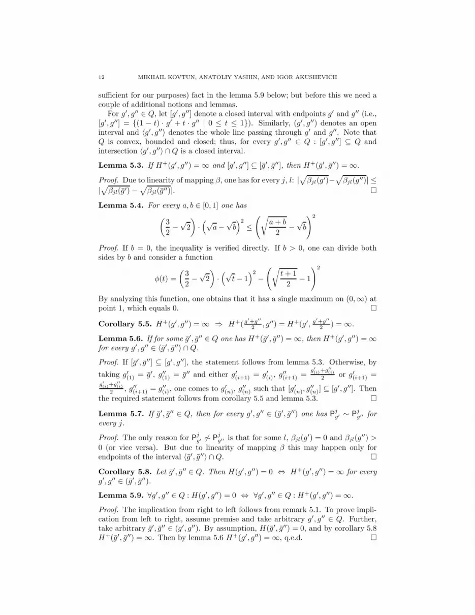
sufficient for our purposes) fact in the lemma 5.9 below; but before this we need acouple of additional notions and lemmas.

For g′, g′′ ∈ Q, let [g′, g′′] denote a closed interval with endpoints g′ and g′′ (i.e.,[g′, g′′] = (1 − t) · g′ + t · g′′ | 0 ≤ t ≤ 1). Similarly, (g′, g′′) denotes an openinterval and 〈g′, g′′〉 denotes the whole line passing through g′ and g′′. Note thatQ is convex, bounded and closed; thus, for every g′, g′′ ∈ Q : [g′, g′′] ⊆ Q andintersection 〈g′, g′′〉 ∩Q is a closed interval.

Lemma 5.3. If H+(g′, g′′) = ∞ and [g′, g′′] ⊆ [g′, g′′], then H+(g′, g′′) = ∞.

Proof. Due to linearity of mapping β, one has for every j, l: |√βjl(g′)−

√βjl(g′′)| ≤

|√βjl(g′) −

√βjl(g′′)|.

Lemma 5.4. For every a, b ∈ [0, 1] one has

(3

2−√

2

)·(√

a−√b)2

≤(√

a+ b

2−√b

)2

Proof. If b = 0, the inequality is verified directly. If b > 0, one can divide bothsides by b and consider a function

φ(t) =

(3

2−√

2

)·(√

t− 1)2

−(√

t+ 1

2− 1

)2

By analyzing this function, one obtains that it has a single maximum on (0,∞) atpoint 1, which equals 0.

Corollary 5.5. H+(g′, g′′) = ∞ ⇒ H+(g′+g′′

2 , g′′) = H+(g′, g′+g′′

2 ) = ∞.

Lemma 5.6. If for some g′, g′′ ∈ Q one has H+(g′, g′′) = ∞, then H+(g′, g′′) = ∞for every g′, g′′ ∈ 〈g′, g′′〉 ∩Q.

Proof. If [g′, g′′] ⊆ [g′, g′′], the statement follows from lemma 5.3. Otherwise, by

taking g′(1) = g′, g′′(1) = g′′ and either g′(i+1) = g′(i), g′′(i+1) =

g′

(i)+g′′

(i)

2 or g′(i+1) =g′

(i)+g′′

(i)

2 , g′′(i+1) = g′′(i), one comes to g′(n), g′′(n) such that [g′(n), g

′′(n)] ⊆ [g′, g′′]. Then

the required statement follows from corollary 5.5 and lemma 5.3.

Lemma 5.7. If g′, g′′ ∈ Q, then for every g′, g′′ ∈ (g′, g′′) one has Pjg′ ∼ P

jg′′ for

every j.

Proof. The only reason for Pjg′ 6∼ P

jg′′ is that for some l, βjl(g

′) = 0 and βjl(g′′) >

0 (or vice versa). But due to linearity of mapping β this may happen only forendpoints of the interval 〈g′, g′′〉 ∩Q.

Corollary 5.8. Let g′, g′′ ∈ Q. Then H(g′, g′′) = 0 ⇔ H+(g′, g′′) = ∞ for everyg′, g′′ ∈ (g′, g′′).

Lemma 5.9. ∀g′, g′′ ∈ Q : H(g′, g′′) = 0 ⇔ ∀g′, g′′ ∈ Q : H+(g′, g′′) = ∞.

Proof. The implication from right to left follows from remark 5.1. To prove impli-cation from left to right, assume premise and take arbitrary g′, g′′ ∈ Q. Further,take arbitrary g′, g′′ ∈ (g′, g′′). By assumption, H(g′, g′′) = 0, and by corollary 5.8H+(g′, g′′) = ∞. Then by lemma 5.6 H+(g′, g′′) = ∞, q.e.d.


5.2. Tail space. In this and subsequent subsections we consider random vari-ables Xj as defined on measurable space (A,B(A)); thus,the σ-algebras Fn =σ(X1, . . . , Xn), F∞ = σ(

⋃n Fn), F∞

n = σ(Xn, Xn+1, . . . ), and X =⋂

n F∞n ) are

subalgebras of B(A).Consider a relation ∼ on A defined as:

(13) a′ ∼ a′′def

= ∃n∀m > n : a′m = a′′m

Obviously, this relation is an equivalence relation; let a denote a coset of a ∈ A,

and A denote a factorspace of A.

Unfortunately, the factor topology of A is trivial (a closure of every one-point setis the whole space), and thus does not possess any useful for our purpose property.

One can easily verify that for every A ∈ X the implication a ∈ A ⇒ a ⊆ Aholds, and that for every a ∈ A the coset a belongs to the tail σ-algebra X. This

makes the tail σ-algebra X isomorphic to its image X = A ⊆ A | ∃A ∈ X :

A = a | a ∈ A under factor mapping. Any measure P on (A,B(A)) can be

restricted to σ-algebra X; this restriction gives rise to measure P on (A, X). Also,

any X-measurable function f on A corresponds to a X-measurable function f on A

defined as f(a) = f(a).

The measurable space (A, X) is called a tail space. The slight advantage of

considering the tail space instead of (A,X) is that atoms of X (in the sense ofBoolean algebra) are one-point sets, while atoms of X are cosets of relation ∼.

In the subsequent subsections, we drop the ∼ sign and use A, X, etc. to denote

A, X, etc. This should not led to confusion, as any statement regarding (A, X)can be reformulated as a statement regarding (A,X), and in the most cases suchreformulation consists just of dropping ∼ sign.

5.3. Orthogonality of measures restricted to X. For every measures P′, P

′′

on (A,B(A)) the absolute continuity P′ ≪ P

′′ implies the absolute continuity ofmeasures restricted to X, P

′|X ≪ P′′|X. We shall show that a similar implication

holds for orthogonality in the case of family of measures Pgg∈Q. Namely:

Lemma 5.10. Suppose that ∀g′, g′′ ∈ Q : g′ 6= g′′ ⇒ Pg′ ⊥ Pg′′ . Then ∀g′, g′′ ∈Q : g′ 6= g′′ ⇒ Pg′ |X ⊥ Pg′′ |X, i.e. there exist A ∈ X such that Pg′(A) = 1 andPg′′(A) = 0.

Proof. Assume premise of the lemma. By lemma 5.9,

∑∞j=1

∑l

(√βjl(g′) −

√βjl(g′′)

)2

diverges for every g′ 6= g′′. This implies that for every n the sum

∑∞j=n

∑l

(√βjl(g′) −

√βjl(g′′)

)2

also diverges. From this, by applying considerations of subsection 5.1 to the space

A(n) =∏∞

j=n1, . . . , Lj, one obtains P(n)g′ ⊥ P

(n)g′′ for arbitrary g′ 6= g′′ (here P

(n)g

denotes a measure on A(n) defined in the way similar to the definition of Pg on

A). But P(n)g′ and P

(n)g′′ are marginals of Pg′ and Pg′′ , respectively; thus, for every n

there exists a set An ∈ F∞n such that Pg′(An) = 1 and Pg′′(An) = 0.

Now take A =⋂∞

n=1

⋃∞j=n An. It is easy to verify that A ∈ X and Pg′(A) = 1,

Pg′′(A) = 0, which proves the lemma.


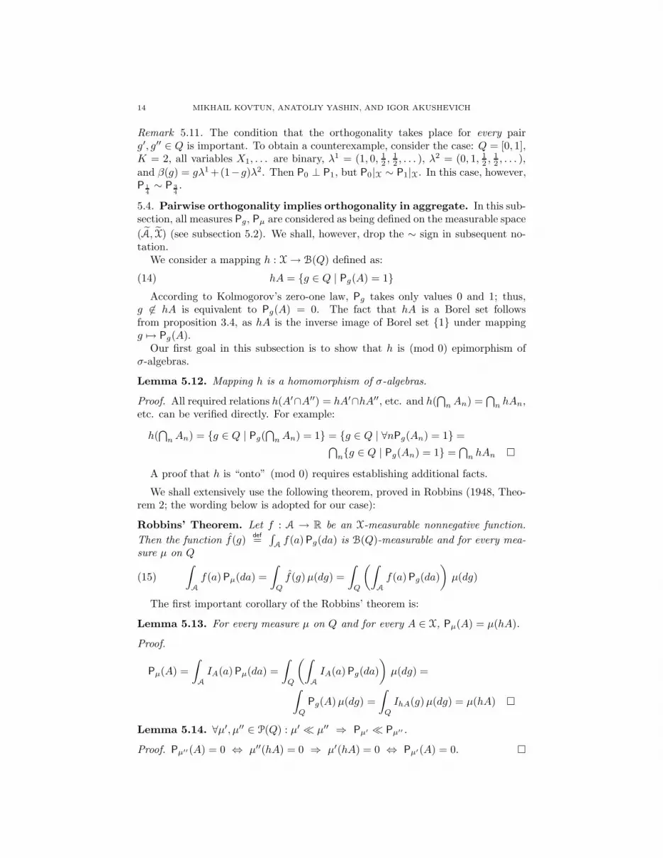
Remark 5.11. The condition that the orthogonality takes place for every pairg′, g′′ ∈ Q is important. To obtain a counterexample, consider the case: Q = [0, 1],K = 2, all variables X1, . . . are binary, λ1 = (1, 0, 1

2 ,12 , . . . ), λ

2 = (0, 1, 12 ,

12 , . . . ),

and β(g) = gλ1 +(1−g)λ2. Then P0 ⊥ P1, but P0|X ∼ P1|X. In this case, however,P 1

4∼ P 3

4.

5.4. Pairwise orthogonality implies orthogonality in aggregate. In this sub-section, all measures Pg, Pµ are considered as being defined on the measurable space

(A, X) (see subsection 5.2). We shall, however, drop the ∼ sign in subsequent no-tation.

We consider a mapping h : X → B(Q) defined as:

(14) hA = g ∈ Q | Pg(A) = 1According to Kolmogorov’s zero-one law, Pg takes only values 0 and 1; thus,

g 6∈ hA is equivalent to Pg(A) = 0. The fact that hA is a Borel set followsfrom proposition 3.4, as hA is the inverse image of Borel set 1 under mappingg 7→ Pg(A).

Our first goal in this subsection is to show that h is (mod 0) epimorphism ofσ-algebras.

Lemma 5.12. Mapping h is a homomorphism of σ-algebras.

Proof. All required relations h(A′∩A′′) = hA′∩hA′′, etc. and h(⋂

nAn) =⋂

n hAn,etc. can be verified directly. For example:

h(⋂

nAn) = g ∈ Q | Pg(⋂

nAn) = 1 = g ∈ Q | ∀nPg(An) = 1 =⋂

ng ∈ Q | Pg(An) = 1 =⋂

n hAn

A proof that h is “onto” (mod 0) requires establishing additional facts.

We shall extensively use the following theorem, proved in Robbins (1948, Theo-rem 2; the wording below is adopted for our case):

Robbins’ Theorem. Let f : A → R be an X-measurable nonnegative function.

Then the function f(g)def

=∫

Af(a)Pg(da) is B(Q)-measurable and for every mea-

sure µ on Q

(15)

∫

A

f(a)Pµ(da) =

∫

Q

f(g)µ(dg) =

∫

Q

(∫

A

f(a)Pg(da)

)µ(dg)

The first important corollary of the Robbins’ theorem is:

Lemma 5.13. For every measure µ on Q and for every A ∈ X, Pµ(A) = µ(hA).

Proof.

Pµ(A) =

∫

A

IA(a)Pµ(da) =

∫

Q

(∫

A

IA(a)Pg(da)

)µ(dg) =

∫

Q

Pg(A)µ(dg) =

∫

Q

IhA(g)µ(dg) = µ(hA)

Lemma 5.14. ∀µ′, µ′′ ∈ P(Q) : µ′ ≪ µ′′ ⇒ Pµ′ ≪ Pµ′′ .

Proof. Pµ′′(A) = 0 ⇔ µ′′(hA) = 0 ⇒ µ′(hA) = 0 ⇔ Pµ′(A) = 0.


Lemma 5.15. Let µ′, µ′′ ∈ P(Q) be such that Pµ′ ≪ Pµ′′ . Then there exists ameasure µ′′ ∈ P(Q) such that µ′′ ≪ µ′′ and Pµ′′ = Pµ′ .

Proof. Let

z(a) =dPµ′

dPµ′′

(a)

be a Radon-Nikodym derivative of Pµ′ with respect to Pµ′′ . Let us fix any variant ofz(a). By Robbins’ theorem, the function y(g) =

∫Az(a)Pg(da) is B(Q)-measurable

and∫

Q

y(g)µ′′(dg) =

∫

Q

(∫

A

z(a)Pg(da)

)µ′′(dg) =

∫

A

z(a)Pµ′′(da) = 1

Thus, the set function µ′′(B)def

=∫

By(g)µ′′(dg) is a probabilistic measure on Q

and µ′′ ≪ µ′′. Further, using lemma 5.13 and Robbins’ theorem, one obtains forarbitrary A ∈ X:

Pµ′′(A) = µ′′(hA) =

∫

Q

IhA(g)y(g)µ′′(dg) =

∫

Q

IhA(g)

(∫

A

z(a)Pg(da)

)µ′′(dg)

(∗)=

∫

Q

(∫

A

IA(a)z(a)Pg(da)

)µ′′(dg) =

∫

A

IA(a)z(a)Pµ′′(da) = Pµ′(A)

The intermediate equality (∗) is verified directly:

Pg(A) = 1 ⇒ IhA(g) = 1 and

∫

A

z(a)Pg(da) =

∫

A

z(a)Pg(da)

and

Pg(A) = 0 ⇒ IhA(g) = 0 and

∫

A

z(a)Pg(da) = 0

Thus, one obtains Pµ′′ = Pµ′ , q.e.d. We did not prove that different variants ofz(a) lead to the same measure µ′′, but it is insignificant for this lemma, as it claimsonly existence of measure µ′′ with desired properties, and any variant of z(a) givessuch example.

Lemma 5.16. Suppose that ∀g′, g′′ ∈ Q : g′ 6= g′′ ⇒ Pg′ ⊥ Pg′′ . Then continuityof µ ∈ P(Q) implies continuity of Pµ.

Proof. Assume, in contrary, that A0 ∈ X is an atom of Pµ, i.e. Pµ(A0) > 0 and forevery A ∈ X, A ⊆ A0, either Pµ(A) = Pµ(A0) or Pµ(A) = 0.

Let B0 = hA0. Then µ(B0) > 0, and we can consider a measure µ0 = µ(·|B0).It is easy to see that Pµ0 is carried by A0 and A0 is an atom of Pµ0 .

Consider any measure µ′ ≪ µ0. By lemma 5.14, Pµ′ ≪ Pµ0 . Thus, there existsa Radon-Nikodym derivative z(a) = dPµ′/dPµ0 . But as A0 is atom of Pµ0 , z(a) isPµ0 -a.s. a constant on A0, and it follows from normalization conditions that thisconstant is 1. Thus, Pµ′ = Pµ0 for every measure µ′ ≪ µ0.

Now return to the set B0. As µ0(B0) = 1 and µ0 has no atoms, it is possible toconstruct two sequences of subsets of B0, B′

nn and B′′nn, such that B′

n g′,B′′

n g′′, g′ 6= g′′, and µ0(B′n) > 0, µ0(B

′′n) > 0 for all n.


Consider measures µ′n = µ0(·|B′

n) and µ′′n = µ0(·|B′′

n). One has µ′n

w−→ δg′ and

µ′′n

w−→ δg′′ , while Pµ′

n= Pµ′′

n= Pµ0 for all n. From continuity of the mixing operator

(Kovtun, 2005), one obtains

Pg′ = limn→∞

Pµ′

n= lim

n→∞Pµ′′

n= Pg′′

which contradicts to the assumption of the lemma that Pg′ ⊥ Pg′′ .

Lemma 5.17. Suppose that ∀g′, g′′ ∈ Q : g′ 6= g′′ ⇒ Pg′ ⊥ Pg′′ . Let µ ∈ P(Q) bea continuous measure. Then Pµ ⊥ Pg for every g ∈ Q.

Proof. Assume premise of the lemma and take arbitrary continuous µ and arbitraryg. Let µ = 1

2 (µ + δg). Due to linearity of the mixing operator, Pµ = 12 (Pµ + Pg),

and thus Pµ ≪ Pµ and Pg ≪ Pµ. Let

z(a) =dPµ

dPµ(a), z(a) =

dPg

dPµ(a), A0 = a | z(a) · z(a) > 0

Then Pµ ⊥ Pg is equivalent to Pµ(A0) = 0.Assume in contrary that Pµ(A0) > 0. Take arbitrary A1 ⊆ A0. If 0 < Pµ(A1) <

Pµ(A0), then Pg(A1) > 0 and Pg(A0 \ A1) > 0, which contradicts to the Kol-mogorov’s zero-or-one law. Thus, A0 is an atom of Pµ, and consequently an atomof Pµ, which contradicts to the lemma 5.16.

Lemma 5.18. Suppose that ∀g′, g′′ ∈ Q : g′ 6= g′′ ⇒ Pg′ ⊥ Pg′′ . Let µ ∈ P(Q) bea continuous measure, and µ′ ∈ P(Q) be a counting measure. Then Pµ ⊥ Pµ′ .

Proof. Any counting measure can be represented in form µ′ =∑∞

i=1 aiδgi, where

ai ≥ 0 and∑ai = 1. Then due to linearity of the mixing operator Pµ′ =

∑aiPgi

.For every i = 1, . . . take Ai such that Pµ(Ai) = 1 and Pgi

(Ai) = 0 (such sets existdue to lemma 5.17). Now take A =

⋂i Ai. Then Pµ(A) = 1 and Pµ′(A) = 0.

Lemma 5.19. Suppose that ∀g′, g′′ ∈ Q : g′ 6= g′′ ⇒ Pg′ ⊥ Pg′′ . Let µ ∈ P(Q) bea continuous measure, F be a closed set such that µ(F ) > 0, µ′ = µ(·|F ), and z(a)be a Radon-Nikodym derivative of Pµ′ with respect to Pµ. Let A0 = a | z(a) > 0.Then µ(F hA0) = 0.

Proof. As µ′(hA0) = Pµ′(A0) = 1, one obtains µ′(F \ hA0) = 0; consequently,µ(F \ hA0) = 0.

Next, assume in contrary that µ(hA0 \F ) > 0. As F is closed, one can constructa sequence of sets Bnn such that B′′

n ⊆ hA0 \ F , µ(Bn) > 0, and Bn g forsome g ∈ hA0 \F . Let µn = µ(·|Bn). Then µn ≪ µ, and by lemma 5.14 Pµn

≪ Pµ.Let

zn(a) =dPµn

dPµ(a), An = a | zn(a) > 0

It is always possible to choose such variants of zn(a) that An ⊆ A0, An+1 ⊆ An.Let B′

n = hAn ∩ F . Then B′n+1 ⊆ B′

n and µ′(B′n) = µ′(hAn) = Pµ′(An) > 0 (as

Pµ′(An) = 0 ⇔ Pµ(An) = 0).Let µ′

n = µ′(·|B′n). We claim that Pµ′

n≪ Pµn

. To prove this, take any set Asuch that Pµ′

n(A) > 0; then Pµ′

n(A) = µ′

n(hA) = µ′n(hA ∩ hAn) = Pµ′

n(A ∩ An);

further, as µ′n ≪ µ′ ≪ µ, Pµ(A ∩ An) > 0, and consequently Pµn

(A ∩ An) > 0,q.e.d.

Further, we claim that there exists a point g′ ∈ F such that ∀ ε > 0 ∀n :µ′

n(Uεg′) > 0. To prove this, suppose the contrary, i.e. that for every point g ∈ F


there exists ε(g) such that µ′n(Uε(g)g) = 0 for all n starting some n(g) (note that

for n′ > n one has µ′n′ ≪ µ′

n, and thus µ′n(U) = 0 ⇒ µ′

n′(U) = 0). This systemcovers F , and as F is compact, it contains a finite subcover Uε(gi)gim

i=1. Letn0 = max(n(g1), . . . , n(gm)). Then 1 = µ′

n0(F ) ≤ ∑

i µ′n0

(Uε(gi)gi) = 0. Thiscontradiction proves the claim.

Now take B′′n = B′

n ∩ U1/ng′ ∪ g′ and µ′′

n = µ′n(·|B′′

n). One has B′′n g′.

As µ′′n ≪ µ′

n, one obtains Pµ′′

n≪ Pµ′

n≪ Pµn

. By lemma 5.15, one can constructmeasures µn ≪ µn such that Pµn

= Pµ′′

n. Finally, using continuity of the mixing

operator (Kovtun, 2005), one obtains

Pg′ = limn→∞

Pµ′′

n= lim

n→∞Pµn

= Pg

which contradicts to the assumption of the lemma that Pg′ ⊥ Pg.

Lemma 5.20. Suppose that ∀g′, g′′ ∈ Q : g′ 6= g′′ ⇒ Pg′ ⊥ Pg′′ . Then for everycontinuous measure µ ∈ P(Q) and for every B ∈ B(Q) there exists A ∈ X such thatµ(B hA) = 0.

Proof. Take arbitrary continuous µ ∈ P(Q). Let B0 = B ∈ B(Q) | ∃A ∈ X :µ(B hA) = 0. By lemma 5.19, all closed subsets of Q belong to B0. Ash is a homomorphism of σ-algebras (lemma 5.12), B0 is closed under finite andcountable unions and intersections and under complements. Thus, B0 coincideswith B(Q).

Lemma 5.21. Suppose that ∀g′, g′′ ∈ Q : g′ 6= g′′ ⇒ Pg′ ⊥ Pg′′ . Then for everycounting measure µ ∈ P(Q) and for every B ∈ B(Q) there exists A ∈ X such thatµ(B hA) = 0.

Proof. Let µ =∑∞

i=1 aiδgi, where ai ≥ 0 and

∑ai = 1. Then Pµ =

∑aiPgi

.For every n 6= m take Anm such that Pgn

(Anm) = 1 and Pgm(Anm) = 0, and

take An =⋂

m 6=nAnm. Then Pgn(An) = 1 and for every m 6= n Pgm

(An) = 0.

Now for every B ∈ B(Q) take AB =⋃An | gn ∈ B. It is easy to verify that

µ(B hAB) = 0.

Lemma 5.22. Suppose that ∀g′, g′′ ∈ Q : g′ 6= g′′ ⇒ Pg′ ⊥ Pg′′ . Then forevery measure µ ∈ P(Q) and for every B ∈ B(Q) there exists A ∈ X such thatµ(B hA) = 0.

Proof. Every measure µ on Q can be represented as αµ′ + (1 − α)µ′′, where µ′ iscontinuous and µ′′ is counting.

By lemma 5.18, one can find sets A′, A′′ ∈ X such that Pµ′(A′) = 1, Pµ′′(A′′) = 1,and A′ ∩A′′ = ∅.

Now take arbitrary B ∈ B(Q). By lemma 5.20, there exists A1 ∈ X such thatµ′(BhA1) = 0, and by lemma 5.21, there exists A2 ∈ X such that µ′′(BhA2) =0. It is always possible to choose these sets such that A1 ⊆ A′ and A2 ⊆ A′′. Thus,A1 ∩A2 = ∅ and µ′(hA2) = µ′′(hA1) = 0.

Finally,

µ(B h(A1 ∪A2)) = µ(B hA1 hA2) =

αµ′(B hA1 hA2) + (1 − α)µ′′(B hA1 hA2) =

αµ′(B hA1) + (1 − α)µ′′(B hA2) = α · 0 + (1 − α) · 0 = 0

Lemma 5.22 allows us to obtain a corollary which is of interest by itself. Namely:


Lemma 5.23. Suppose that ∀g′, g′′ ∈ Q : g′ 6= g′′ ⇒ Pg′ ⊥ Pg′′ . Then ∀µ1, µ2 ∈P(Q) : µ1 ⊥ µ2 ⇒ Pµ1 ⊥ Pµ2 .

Proof. Assume premise of the lemma and take arbitrary µ1, µ2 such that µ1 ⊥ µ2.Then there exists Borel B1, B2 ⊆ Q such that µ1(B1) = 1, µ2(B2) = 1, andB1 ∩B2 = ∅.

Let µ = 12 (µ1 + µ2). By lemma 5.22 there exist sets A′

1, A′2 ∈ X such that

µ(B1hA′1) = µ(B2hA′

2) = 0. As Pµ(A′1∩A′

2) = µ(hA′1∩hA′

2) = µ(B1∩B2) = 0,the sets A1 = A′

1 \ (A′1 ∩A′

2) and A2 = A′2 \ (A′

1 ∩A′2) also satisfy µ(B1 hA1) =

µ(B2 hA2) = 0.Now one has Pµ1(A1) = µ1(hA1) = µ1(B1) = 1; similarly, Pµ2(A2) = 1. As A1

and A2 are disjoint, one obtains orthogonality of Pµ1 and Pµ2 .

On the other hand, lemma 5.22 can be easily derived from lemma 5.23. Forthis, take arbitrary µ ∈ P(Q) and B ∈ B(Q). If µ(B) = 1 or µ(B) = 0, one cantake A = A or A = ∅, respectively. Otherwise, one can consider measures µ(·|B)and µ(·|Q \ B). These measures are orthogonal, and by lemma 5.23 measuresPµ(·|B) and Pµ(·|Q\B) are orthogonal as well. Take A such that Pµ(·|B)(A) = 1 andPµ(·|Q\B)(A) = 0. It is easy to see that µ(B hA) = 0, which proves lemma 5.22.

Lemma 5.22 shows that for every µ ∈ P(Q) the metric structure of spaces(Q,B(Q), µ) and (A,X,Pµ) are isomorphic. This allows us to employ Rokhlin’stechnique (see Rokhlin, 1949; Rohlin, 1952) to obtain the main result of the presentsubsection.

As Q is a complete separable metric space, (Q,Bµ(Q), µ) is a Lebesgue spacefor every Borel measure µ (recall that Bµ(Q) denotes a Lebesgue completion ofBorel σ-algebra B(Q) with respect to measure µ, and µ denotes the correspondingcompletion of measure µ).

Let us fix some measure µ on (Q,B(Q)), and let G = Γi∞i=1 be a topology base

of Q; it is also a Rokhlin’s basis of (Q,Bµ(Q), µ). Let further Γi be a coset of Γi

by ideal of µ-negligible sets Iµ.

By lemma 5.22, there exists a set Ci ∈ X such that hCi ∈ Γi. Let ∆i = ΓihCi,and let Q0 =

⋃∞i=1 ∆i, Q1 = Q \Q0. Then we have exact equalities hCi = Γi ∩Q1

and h(A \ Ci) = Q1 \ Γi.Note that both Q0 and Q1 are Borel sets (as all Γi are open, and all hCi are

Borel).For arbitrary g ∈ Q1, let Υi(g) = Γi∩Q1 if g ∈ Γi, and Υi(g) = Q1 \Γi if g 6∈ Γi.

Correspondingly, let Di(G) = Ci if g ∈ Γi, and Di(g) = A \ Ci if g 6∈ Γi. ThenhDi(g) = Υi(g).

Finally, let Ag =⋂

i Di(g). As h is homomorphism of σ-algebras, one obtainshAg = h(

⋂i Di(g)) =

⋂i hDi(g) =

⋂i Υi(g) = g. This means that Pg(Ag) = 1

and for every g′ 6= g, Pg′(Ag) = 0. Thus, we proved:

Lemma 5.24. Suppose that ∀g′, g′′ ∈ Q : g′ 6= g′′ ⇒ Pg′ ⊥ Pg′′ . Then for everymeasure µ ∈ P(Q) there exists a Borel subset Q1 ⊆ Q of full measure, µ(Q1) = 1,and a mapping ψ : Q1 → X : g 7→ Ag satisfying (a) ∀ g ∈ Q1 : Pg(Ag) = 1 and (b)∀ g, g′ ∈ Q1 : g 6= g′ ⇒ Ag ∩Ag′ = ∅.

As sets Agg∈Q1 are disjoint, one can consider a mapping A → Q : a 7→ ga,defined as ga = g, if a ∈ Ag, and ga = g0 for a 6∈

⋃g∈Q1

Ag; g0 ∈ Q is taken


arbitrarily. It is easy to see that the mapping a 7→ ga is B(Q)-X-measurable. Thus,we have

Lemma 5.25. Suppose that ∀g′, g′′ ∈ Q : g′ 6= g′′ ⇒ Pg′ ⊥ Pg′′ . Then for everymeasure µ ∈ P(Q) there exists a Borel subset Q1 ⊆ Q of full measure, µ(Q1) = 1,and a B(Q)-X-measurable mapping ϕ : A → Q : a 7→ ga satisfying Q1 ⊆ ϕ(A) andPg(ϕ

−1(g)) = 1 for every g ∈ Q1.

5.5. Conditional probabilities with respect to tail σ-algebra. Let P be aprobabilistic measure on (A,B(A)). We say that P satisfies 0-1-law, if for everyA ∈ X either P(A) = 1 or P(A) = 0.

Note that all measures Pg, g ∈ Q, satisfy 0-1-law.For measures satisfying 0-1-law, conditional probabilities with respect to tail

σ-algebra X can be expressed directly. Namely, a well-known fact is:

Lemma 5.26. Let measure P satisfy 0-1-law. Then for every B ∈ B(A) one hasP(B|X)(a) = P(B) for P-almost all a ∈ A.

With this we can easily prove:

Lemma 5.27. Suppose that ∀g′, g′′ ∈ Q : g′ 6= g′′ ⇒ Pg′ ⊥ Pg′′ . Then for everymeasure µ ∈ P(Q) there exists a Borel set Q1 of full measure, µ(Q1) = 1, such thattail σ-algebra X is sufficient for the family Pgg∈Q1 .

Proof. Take Q1 satisfying conditions of lemma 5.25. For a ∈ A and B ∈ B(A), let

P (a,B)def

= Pϕ(a)(B) (where ϕ was defined in lemma 5.25). By definition, P (a,B) isa probabilistic measure on (A,B(A)) for every fixed a ∈ A. Further, by proposition3.4 and lemma 5.25, P (a,B) is X-measurable as function of a for every fixed B,and by lemma 5.25, for every g ∈ Q1 and for every fixed B, P (a,B) = Pg(B)for Pg-almost all a. Finally, by lemma 5.26, P (a,B) = Pg(B|X)(a) Pg-a.s., whichcompletes the proof.

The inverse statement is also true:

Lemma 5.28. Suppose that for every measure µ ∈ P(Q) there exists a Borel setQ1 of full measure, µ(Q1) = 1, such that tail σ-algebra X is sufficient for the familyPgg∈Q1 . Then ∀g′, g′′ ∈ Q : g′ 6= g′′ ⇒ Pg′ ⊥ Pg′′ .

Proof. Take arbitrary g′, g′′ ∈ Q such that g′ 6= g′′ and consider a measure µ =12 (δg′ + δg′′ ). Then any set Q1 of full measure µ contains g′ and g′′. Sufficiencyof X means that there exists a function P (a,B) such that Pg′(B|X)(a) = P (a,B)Pg′ -a.s. and Pg′′(B|X)(a) = P (a,B) Pg′′ -a.s. Family Pgg∈Q consists of distinctmeasures; thus, there exists a set B0 ∈ B(A) such that Pg′(B0) 6= Pg′′(B0).

Take A′ = a | P (a,B0) = Pg′(B0) and A′′ = a | P (a,B0) = Pg′′(B0). Byconstruction, A′ ∩ A′′ = ∅, and by lemma 5.26, Pg′(A′) = Pg′′ (A′′) = 1, whichproves orthogonality of Pg′ and Pg′′ .

6. Discussion

6.1. Orthogonality in aggregate: for “all” or “almost all” g ∈ Q? Theresult proven in lemma 5.24 can be reformulated as “pairwise orthogonality ofmeasures Pgg∈Q implies orthogonality in aggregate for almost all measures fromthis family.” The “almost all” clause of the above statement can be based on anymeasure µ on Q—note, however, that sets Ag may depend on the choice of µ.


One can also see that there is no obvious modification of our proof, which givesorthogonality in aggregate for the whole family Pgg∈Q.

A natural question arise: whether the absence of full orthogonality in aggregateis an immanent property or it is merely a deficiency of our proof?

This question can be also formulated in terms of lemma 5.22, which states thathomomorphism h : X → B(Q) is “onto” (mod 0); again, “(mod 0)” holds for anymeasure µ on Q—and again, set A satisfying µ(B A) = 0 may depend on thechoice of µ. This point of view can be (less formally) expressed as: is the tailσ-algebra X sufficiently rich to have a factor-algebra isomorphic to B(Q), or onecan obtain only isomorphism (mod 0)?

6.2. Structure of tail σ-algebras. Structure of tail σ-algebras deserved not toomuch attention. Such lack of interest can be explained, first, by the fact that tail σ-algebras are “trivial” from probabilistic point of view (any independent distribution,being restricted to the tail σ-algebra, takes only values 0 and 1), and second, by theabsence of topology or other “good” structure generating tail σ-algebras (cf., forexample, a comprehensive study of Borel sets by means of topology and descriptiveset theory).

A study performed in the present paper demonstrates that an explicit investiga-tion of properties of tail σ-algebra might bring fruitful results: technical basis for ourmain theorem is existence of homomorphism h : X → B(Q), which is epimorphism(mod 0), proved in lemma 5.22. An important corollary of the latest fact is thatfor every measure µ on (Q,B(Q)) the metric structures of spaces (Q,B(Q), µ) and(A,X,Pµ) are isomorphic.

Note that X is constructed from ranges of random variablesX1, . . . ; nothing fromdistribution of X1, . . . is involved in construction of X. Lemma 5.22 establishesexistence of homomorphism h for any set Q—provided that Q is compact andcontinuously parameterize pairwise orthogonal family of independent measures. Inother words, X is universal with respect to family of σ-algebras B(Q)Q. It lookslike this universality is a characteristic property of tail σ-algebras, and might be auseful tool for further investigation of their properties.

6.3. Connection with the strong law of large numbers. One fact that wehave proved in this article is that pairwise orthogonality of considered family of in-dependent distributions implies their orthogonality in aggregate. Informally speak-ing, one can say the sets Ag, provided by lemma 5.24 are “sufficiently small” to bedisjoint.

Another way to obtain “small” sets with Pg measure 1 is provided by the stronglaw of large numbers. In some sense, the “smallness” of the set of outcomes providedby the strong law of large numbers is one of cornerstones of probability theory.When random variables Xj are identically distributed for every g, the sets givenby the law of large numbers for different Pg are disjoint.

Consider, however, the following example.Let Xj be a sequence of binary random variables taking values 0 and 1, Q =

[−1, 1], and for every g ∈ Q, Pg(Xj = 1) = 12 + g

2√

jand Pg(Xj = 0) = 1

2 −g

2√

j. It is

easy to verify that condition (9) of the main theorem is satisfied; thus, distributionsPg are pairwise orthogonal. Now from lemma 5.24 one obtains existence of a disjointfamily of sets Agg∈Q1 (whereQ1 has Lebesgue measure 1, and thus has cardinalityof continuum) such that Pg(Ag) = 1.


The strong law of large numbers in form of Kolmogorov (Shiryaev, 2004, IV.3.2),adopted for our case, states that for every increasing unbounded sequence of positivereals bnn such that

∑∞1

1b2n<∞ the set

A(LN)g = a ∈ A |

∑n1 aj−

∑n1 Pg(Xj=1)

bn→ 0

has Pg probability 1.

Using the facts that∑∞

11b2n<∞ implies that

√n

bn→ 0 and that

n∑

1

Pg(Xj = 1) −n∑

1

Pg′(Xj = 1) =

n∑

1

g − g′

2√j

= O(√n)

one obtains that A(LN)g = A

(LN)g′ for all g, g′ ∈ Q.

Thus, the strong law of large numbers may produce sets of probability 1 thatcan be made “significantly smaller”—namely, the set produced by the strong lawof large numbers can be splitted into continuum of subsets, each of which hasprobability 1 with respect to corresponding distribution.

We believe that further investigation of consequences of this fact might bringinteresting results.

6.4. Constructiveness of proofs. The proof of existence of set Ag in lemma5.24 is non-constructive; moreover, it explicitly uses axiom of choice. It would bedesirable to find a constructive description of sets Ag (e.g., as in the strong lawof large numbers), as it would simplify analysis of their properties. In particular,we expect that constructive description of sets Ag would clarify the answer to thequestion of section 6.1.

7. Acknowledgements

The first author personally thanks professor James N. Siedow (Vice Provost forResearch, Duke University), whose trust in the author made this work possible.

References

Dellacherie, C. and Meyer, P.-A. (1978). Probabilities and Potential, volume I.Amsterdam: North-Holland Publishing Co.

Dunford, N. and Schwartz, J. T. (1958). Linear Operators, volume I. NewYork: Interscience Publishers, Inc.

Kolmogorov, A. N. and Fomin, S. V. (1972). Elements of the theory of functionsand functional analysis. Moscow, Russia: Science, 3rd edition. In Russian.

Kovtun, M. (2005). Continuity of the mixing operator. Submitted for publicationto “Statistics and Probability Letters.” Available from e-Print archive arXiv.orgat http://www.arxiv.org, arXiv code math.PR/0508296.

Kovtun, M., Akushevich, I., Manton, K. G. and Tolley, H. D. (2005a).Grade of membership analysis: One possible approach to foundations. To appearin Focus on Probability Theory, Nova Science Publishers. Available from e-Printarchive arXiv.org at http://www.arxiv.org, arXiv code math.PR/0403373.

Kovtun, M., Akushevich, I., Manton, K. G. and Tolley, H. D. (2005b). Lin-ear latent structure analysis: Mixture distribution models with linear constraints.Submitted for publication to “Statistical Methodology.” Available from e-Printarchive arXiv.org at http://www.arxiv.org, arXiv code math.PR/0507025.

http://www.arxiv.org




Robbins, H. (1948). Mixture of distributions. The Annals of Mathematical Sta-tistics 19(3) 360–369.

Rohlin, V. A. (1952). On the fundamental ideas of measure theory. AmericanMathematical Society Translations 71 1–55.

Rokhlin, V. A. (1949). Ob osnovnykh ponjatijakh teorii mery. MatematicheskijSbornik 25(67) 107–150. In Russian.

Shiryaev, A. N. (2004). Probability. Moscow, Russia: MCCSE, 3rd edition. InRussian.

Teicher, H. (1960). On the mixture of distributions. The Annals of MathematicalStatistics 31(1) 55–73.

Vladimirov, D. A. (2002). Boolean Algebras in Analysis, volume 540 of Mathe-matics and its Applications. Dordrecht, Netherlands: Kluwer Academic Publish-ers.

Yashin, A. I. (1982). Convergence of bayesian estimation in adaptive controlschefes. Richerche di Automatica XIII(1) 6–20.

Yashin, A. I. (1986). Continuous time adaptive filtering. IEEE Transactions onAutomatic Control C-31 776–779.

Mikhail Kovtun: Duke University, CDS, 2117 Campus Dr., Durham, NC, 27708

E-mail address: [email protected]

Anatoliy Yashin: Duke University, CDS, 2117 Campus Dr., Durham, NC, 27708


Igor Akushevich: Duke University, CDS, 2117 Campus Dr., Durham, NC, 27708


Documents

Convergence of Estimators in LLS Analysis