Embed Size (px)
Citation preview
Journal of Multivariate Analysis 106 (2012) 118–146
Contents lists available at SciVerse ScienceDirect
Journal of Multivariate Analysis
journal homepage: www.elsevier.com/locate/jmva
Edgeworth expansions for GEL estimatorsGubhinder Kundhi a,∗, Paul Rilstone b
a Department of Economics, Carleton University, 1125 Colonel By Drive, Ottawa, Ontario, K1S 5B6, Canadab Department of Economics, York University, 4700 Keele Street, Toronto, Ontario, M3J 1P3, Canada
a r t i c l e i n f o
Article history:Received 31 October 2010Available online 3 December 2011
AMS subject classifications:60E0560E1062E1791G70
Keywords:Higher order asymptoticsEdgeworth expansionsGeneralized Empirical LikelihoodGeneralized Method of Moments
a b s t r a c t
Finite sample approximations for the distribution functions of Generalized EmpiricalLikelihood (GEL) are derived using Edgeworth expansions. The analytical results obtainedare shown to apply to most of the common extremum estimators used in applied workin an i.i.d. sampling context. The GEL estimators considered include the ContinuousUpdating, Empirical Likelihood and Exponential Tilting estimators. These estimators arepopular alternatives to Generalized Method of Moment (GMM) estimators and their finitesample properties are examined. In a Monte Carlo Experiment, higher order analyticalcorrections provided by Edgeworth approximations work well in comparison to first orderapproximations and improve inferences in finite samples.
© 2011 Elsevier Inc. All rights reserved.
1. Introduction
The higher order asymptotic properties of nonlinear estimators have received substantial attention in the statistics andeconometrics literature recently.Most of these estimators are special cases of eitherGeneralizedMethod ofMoments (GMM)or Generalized Empirical Likelihood (GEL) estimators. However, there still remain some substantial gaps in our knowledgeof their finite sample properties. Recent papers by Rilstone, Srivastava and Ullah [24, henceforth RSU] and Newey andSmith [19, henceforth NS] have derived the first and second order moments of certain nonlinear estimators, includingthose focused on in this paper. However, while these results may be useful for bias and dispersion correction and higherorder efficiency comparisons, they do not allow for departures from normality in the distribution of the estimators. Forthis, an Edgeworth or related expansion is necessary, and to derive these requires knowledge of the higher moments of theestimators. The focus of this paper is to derive these expansions for GEL estimators.
The complexity of standard higher order approximations may make them appear quite forbidding. The derivation ofEdgeworth expansions for multivariate models, not to mention nonlinear, can be quite intimidating. Most such derivations,althoughquite elegant, getmireddown in amorass of tensor andmultivariate notation. One result is that the recent attentionof researchers into approximating the distributions of estimators and test statistics has focused primarily on resamplingtechniques such as the bootstrap and the jackknife. This is ironic, since, to show the validity of resampling techniques, onegenerally needs to first derive an asymptotic expansion of some kind. Analytical expansions such as the Edgeworth areuseful whether one wants to use them directly for improved inferences, or as a device to show the validity of a resamplingtechnique.
The focus for GEL estimators is a k× 1 parameter θ whose true value, θ0, is the unique solution to an l× 1 set of momentconditions E[gi(θ0)] = 0. With l > k we have the well known over identification problem. From a technical standpoint,
∗ Corresponding author.E-mail addresses: [email protected] (G. Kundhi), [email protected] (P. Rilstone).
0047-259X/$ – see front matter© 2011 Elsevier Inc. All rights reserved.doi:10.1016/j.jmva.2011.11.005
G. Kundhi, P. Rilstone / Journal of Multivariate Analysis 106 (2012) 118–146 119
this can make the analysis problematic since approximating the estimators thus involves more equations than unknowns.Various remedies to this problem have been proposed by Newey and McFadden [18], RSU [24] and NS [19], who introducevarious auxiliary parameters to even out the number of parameters and estimating equations. We do so here. Letθ denotea generic estimator. For the GEL estimators, as NS [19] have shown,θ is the solution to a saddle point problem, along withan l × 1 vector of Lagrangian multipliersλ.
Let β ′= (λ′,θ ′)′ where ′ denotes transposition. As one simplification we derive approximations to the distribution
function of τ ′β , where τ is anm× 1 vector of constants, rather thanθ . Apart from greatly simplifying the analysis there aretwo other reasons for doing so. First is that, although in principle one may like to derive the k variate distribution ofθ , inpractice most inferences are focused on linear combinations of the parameter vector. Second, as we show below, since theresults hold for arbitrary τ ∈ ℜ
m, it follows that the joint approximate distribution ofβ can be derived from the approximatedistribution of τ ′β . With these results in hand, the critical points from a Cornish–Fisher expansion follow immediately. Theexpansionswe derive are third order accurate in the usual sense that the expansion includes terms up to and including thosewith a coefficient 1/N where N is the sample size. This allows us to correct for higher order bias, variance, skewness andkurtosis.
To name a few papers on the higher order asymptotic properties of estimators and test statistics, Phillips [21] andBhattacharya and Ghosh [3] have examined the validity of Edgeworth expansions for various estimators. Others, such asPfanzagl and Wefelmeyer [20], Ghosh et al. [8] have examined higher order efficiency of maximum likelihood estimators.Rothenberg [26], McCullagh [17] and Barndorff-Nielson and Cox [2] provide early surveys. Amemiya [1] examined the logitregression model. RSU [24] and Rilstone and Ullah [25] derived third-order stochastic expansions and the second order biasand mean squared error of a wide class of nonlinear estimators. NS [19] have compared the second order bias and varianceof various GEL and GMM estimators.
Wallace [28] developed the Edgeworth expansion for a standardized sample average of observations on a univariaterandom variable. Extensions to multivariate random variables were done by Chambers [6], Sargan [27], Phillips [21] andBhattacharya and Rao [4]. Rothenberg [26], Barndorff-Nielson and Cox [2]and Hall [9] provide detailed discussions on thedevelopment of Edgeworth and Cornish–Fisher expansions. Bhattacharya and Ghosh [3] derived general conditions underwhich the Edgeworth expansion provides a valid approximation to various functions of sample moments. They obtainedasymptotic expansions for distributions of the Maximum Likelihood Estimators (MLEs) and minimum contrast estimatorsby application of their results. Phillips and Park [22] derived the Edgeworth expansion for theWald statistic and Hansen [12]obtained the Edgeworth expansion of the objective function for GMMdistance statistic with nonlinear restrictions. Bravo [5]considered the Edgeworth expansion for themaximumdual likelihood estimator and the empirical likelihood ratio statistic.Linton [16] derived the Edgeworth approximation for the semiparametric instrumental variable estimators and associatedtest statistics.
It is well known that although the optimal (two-step) GMM estimator is asymptotically efficient, its finite sampleproperties can be problematic. Imbens [14] notes that the estimator is not invariant to linear transformations of themomentconditions. Studies such as Hansen [11] have shown that the optimal GMM estimator may have substantial bias in smallersamples. Partly in response to these considerations, other asymptotically efficient estimators have been proposed. Theseinclude the Continuous Updating Estimator (CUE), the Empirical Likelihood (EL) estimator and the Exponential Tilting(ET) estimator. The EL and the ET estimators as discussed by Imbens [14] and Qin and Lawless [23] work well with overidentified models and are appealing for their information-theoretic characteristics. Hansen et al. [13] have shown that theCUE estimator can have smaller bias in finite samples than the optimal GMM estimator. NS [19] have shown that all theseestimators are GEL estimators.
In this paper stochastic expansions for the GEL estimators are derived and used to obtain their Edgeworthapproximations. The Edgeworth approximations for the CUE, EL, ET estimators are subsequently obtained as special casesfor comparison purposes. These analytical results are illustrated using an example of an overidentified model from [23].
Analytical expansions are useful for improved finite sample inferences such as lowering coverage errors of confidenceintervals. Also, higher order approximate moments of the estimators can be obtained by integrating the Edgeworthexpansion, providing more distributional information. These expansions can also enable higher order comparisons suchas discussed in [26]. Edgeworth expansions are usually estimated using sample moments and may not provide perfectlyaccurate numerical approximations. However, even in these cases, the analytical corrections delivered by the higher orderterms in the Edgeworth expansions provide an intuitive explanation and measure of the departure of an estimator’s actualsampling distribution from its asymptotic distribution.
For each of the GEL estimators considered we proceed as follows. We let λ denote the associated Lagrangian multipliers.Put β ′
= (λ′, θ ′) and m = k + l. We consider situations where anm × 1 estimator,β , solves
1N
qi(β) = 0 (1.1)
where qi(β) is a knownm×1 vector-valued function of the observable data and E[qi(β)] = 0 only at β = β0. We elaborateon this in the next section. To sidestep a lengthy itemization of regularity conditions, β is assumed to be consistent. Wederive the first four moments of τ ′β and then specialize for the main cases of interest such as τ ′
= (01×l, α′), where α is an
arbitrary k × 1 vector of constants.
120 G. Kundhi, P. Rilstone / Journal of Multivariate Analysis 106 (2012) 118–146
The discussion is structured as follows. In the next section we further discuss the class of estimators to which our resultsapply and provide the notation and assumptions uponwhich our results are based. Section 3 derives third order Edgeworthsfor a general nonlinear class of estimators. Section 4 specializes these results for GEL estimators. Section 5 provides anillustration. This illustration is used to conduct a Monte Carlo simulation in Section 6. Section 7 concludes.
2. Analytical framework
Since the main intent is to provide simplified Edgeworth expansions for a wide class of estimators, this section willprovide a discussion of how the results (also, by implication, those in RSU [24], and Kundhi and Rilstone [15, henceforth KR])can be applied to many, if not most of the estimators commonly used in applied work, at least if one is willing to assumei.i.d. sampling. All of the results are stated in terms of the estimator’s ‘‘influence function’’. We develop a straightforwardnotation for this.
This class of estimatorswhich solve sets of equations such as (1.1) includesmostMLEs, least squares and other extremumestimators inwhich the average of the qi(β) represents the first order conditions for themaximizer. Other approacheswhichmay be put into this framework by appropriate definition of the moment equations are most GMM estimators and othertwo step estimators which involve a nuisance parameter. Textbook discussions of GMM estimators emphasize that they areapplicable to the ‘‘overidentified’’ case in which one has more estimating equations than parameters to estimate. It is worthemphasizing that the method of moments can be extended to cover many of these estimators.
It is useful to introduce some notational conventions. For an n×mmatrix A, ∥A∥ = Trace[AA′]1/2. When the argument β
of a function is suppressed it is understood that the function is evaluated atβ0 so that, for example, A ≡ A(β0). The Kroneckerproduct is defined in the usual way so that with A = [aij] and a p× qmatrix B, we have A⊗ B = [aijB].
−→A ≡ Vec[A] denotes
the usualmn × 1 vector with the columns of A stacked one upon each other.There are various ways to organize the higher order derivatives of a matrix-valued function. We find the following
approach (used e.g. in RSU [24]) to bemost amenable for defining andmanipulating Taylor series ofmatrix-valued functions.Thematrix of νth order partial derivatives of a matrix A(β) is indicated by
ν A(β) = A(ν)(β). Specifically, if A(β) is an n×1vector function, A(1)(β) is the usual Jacobian whose ith row contains the partials of the ith element of A(β). The matrices ofhigher derivatives are defined recursively so that the jth element of the ith row of A(ν)(β) (a n × mν matrix), is the 1 × mvector a(ν)
lj (β) = ∂a(ν−1)lj (β)/∂β ′. Two useful properties of these definitions, are that, if a(β) = [ai(β)] is a n × 1 vector,
then the ith row of a(1)(β) contains the gradient of ai(β) and the ith row of a(2)(β) contains the transposed vectorizationof the Hessian matrix of ai(β). A third useful property of the method with which we define derivatives is that if A(β) is an
n × 1 vector and B = A′ then B(j)=
−→
A(j)′′
. We define A|j|=
−→A
′ −→A(1)
′
· · ·−→A(j)
′′
. We denote the matrix of derivativesof Awith respect to θ by θ A.
A bar over a function indicates its expectation so that A(β) = E[A(β)]. A tilde over a function indicates its deviationfrom its expectation so that A(β) = A(β) − A(β). Also denote Q = (E
qi(1)
)−1. The ‘‘influence function’’ of these models
is denoted as di(β) = Qqi(β). To avoid any confusion, note that Q is evaluated at β0 and hence is treated as a constant.In addition to consistency, the assumptions used are as follows.
Assumption A. The sth order derivatives of qi(β) exist in a neighborhood of β0, i = 1, 2, . . . and E∥q(s)i (β0)∥
2 < ∞.
Assumption B. For some neighborhood of β0,
1N
q(1)i (β)
−1= OP(1).
Assumption C.q(s)
i (β) − q(s)i (β0)
≤ ∥β − β0∥Mi for some neighborhood of β0 where E |Mi| ≤ C < ∞, i = 1, 2, . . . .
The above assumptions, with s ≥ 1, are sufficient forβ to have an asymptotically normal distribution and√Nβ − β0
→
N (0, V) where V = Edid′
i
. To derive the higher order cumulants and the Edgeworth expansions we will make additional
moment assumptions on the derivatives of di(β) and invoke Cramer’s condition on these derivatives, which basicallyrequires the model contain at least one continuous random variable.
Using Assumptions A–C for various values of s, stochastic approximations toβ were obtained in RSU [24] (and simplifiedsomewhat in KR [15]):β = β0 + a−1/2 + a−1 + a−3/2 + OP
N−2 (2.1)
where
a−1/2 = −1N
di, (2.2)
a−1 =a(1)−1/2a−1/2 −
12di(2)
a−1/2 ⊗ a−1/2
, (2.3)
G. Kundhi, P. Rilstone / Journal of Multivariate Analysis 106 (2012) 118–146 121
a−3/2 =a(1)−1/2a−1 +
12
a(2)−1/2
a−1/2 ⊗ a−1/2
− di(2)
a−1/2 ⊗ a−1
−
16di(3)
a−1/2 ⊗ a−1/2 ⊗ a−1/2
. (2.4)
The usefulness of this result is that each of the terms in (2.1) are simple functions of mean-zero matrices. This greatly
simplifies the analysis ofβ , particularly with i.i.d. observations. Note that a(j)−1/2 = −Q 1
N
(d(j)
i − E[d(j)i ]).
Let η = τ ′Vτ . Our focus is on the scalar: τ ′(β − β0)/√
η/N , an asymptotically pivotal random quantity: in fact it has astandard normal distribution in large samples under the usual regularity conditions.
Note by inspection of Eqs. (2.2)–(2.4) that the quantity τ ′(a−1/2 + a−1 + a−3/2) = τ ′(β − β0) + OP(N−2) can be writtenas a smooth, in fact, cubic, function of the sample averages of the dis and their derivatives. The general validity of Edgeworthexpansions for smooth functions of sample multivariate averages was established by Bhattacharya and Ghosh [3]. In ourcase, the application of this result and others is greatly simplified by the cubic approximation.
3. Edgeworth expansions: general case
Edgeworth expansions of smooth functions of the sample means of random variables are functions of the lower ordercumulants of the random quantities involved. As noted, a−1/2 + a−1 + a−3/2 is a smooth function of the sample mean of thed|2|i s. In principle, one could derive the multivariate Edgeworth expansion for these, but it would be quite complicated. By
focusing on the linear combination, τ ′β , we are able to greatly simplify the derivation of moments and hence the Edgeworthitself. Specifically, put
ξ = ξ0 + ξ−1/2 + ξ−1 (3.1)
where
ξ0 =N/η τ ′a−1/2, ξ−1/2 =
N/η τ ′a−1 and ξ−1 =
N/η τ ′a−3/2. (3.2)
The notation is designed in such a way that terms such as aj and ξj are OP(N−j) in magnitude. Moreover, by inspection,ξ0 has mean zero and unit variance which facilitates many derivations. It is straightforward that the probability distributionof ξ corresponds to that of the scaledβ up to order N−1, which we state more formally in the following lemma.
Lemma 1. Let Assumptions A–C hold for some s ≥ 3. Then
ξ =N/η τ ′(β − β0) + OP
N−3/2 .
Proof. This follows directly from Lemma 3.1 in [24].
To find the third order Edgeworth expansion of the distribution function of ξ weneed the first four cumulants of ξ , discardingterms which are lower than O(N−1). Put τi(β) = τ ′di(β). The cumulants are
κ1 = τ ′B/√
η, B = Λ1 −12d(2)1 VecV, (3.3)
κ2 = 1 +Π
N, Π =
2V2 + V3 + 2V4
η(3.4)
κ3 =
S1 + 32 τ ′Λ6 V τ − τ
(2)1 (V τ ⊗ V τ)
η3/2
(3.5)
κ4 = K1/η2− 3 +
4K2 −
12K3
+ 6
K4 +
14K5 − K6
η2
− 4κ1κ3 − 6Π (3.6)
where
Λ1 = E[d(1)1 d1], Λ2 = E[
τ
(1)′1 τ
(1)1 ], Λ3 = E[τ1d
(1)1 ],
Λ4 = E[τ(2)1 (d1 ⊗ Vτ)], Λ5 = E
τ
(1)1 d(1)
1
Vτ , Λ6 = E[d1τ
(1)1 ],
Λ7 = E[d(1)1 ⊗ d1]Vτ , Λ8 = E[τ1τ
(2)1 ]
−→V1, Λ9 = τ
(3)1
Vτ ⊗
−→V1
,

122 G. Kundhi, P. Rilstone / Journal of Multivariate Analysis 106 (2012) 118–146
S1 = −Eτ 31
, S2 = E
τ 21τ
(1)1
, S3 = E[(d1 ⊗ d1)d′
1]τ ,
S4 = τ ′Ed(1)′
1 d1d′
1
τ , S5 = E[τ 2
1 d′
1],
V2 = −S4 +12τ
(2)1 S3,
V3 = (τB)2 + Vec[Λ6]′Vec[Λ′
6] + Trace [Λ2V] +12τ
(2)1 (V ⊗ V) τ
(2)1
′
− 2τ (2)1 (Im ⊗ V)Vec[Λ6],
V4 = Λ5 + Traceτ ′Λ6Λ6
+ τ ′Λ6B − Trace[d(2)
1 [Vτ ⊗ Λ6]] − τ(2)1 Λ7 + Λ4 +
12Λ8 − τ
(2)1 (Im ⊗ Λ3)
−→V1
− τ(2)1 [Vτ ⊗ Λ1] + τ
(2)1 (d(2)
1 ⊗ Im)(Vτ ⊗−→V1) +
12τ
(2)1
d(2)1
−→V1 ⊗ Vτ
−
12Λ9,
K1 = Eτ 41
,
K2 = 3ηS4 + 3τ ′Λ6S5 + 3S2Vτ − S1τΛ1,
K3 = 3ητ1(2)S3 + 6τ1(2) (Vτ ⊗ S5) − S1τ1(2) −→V1,
K4 = η(τ ′Λ1)
2+ Trace [VΛ2] + Trace [Λ6Λ6]
+ 2
2τ ′Λ6Vττ ′Λ1 + τ ′Λ6VΛ′
6τ + 2τ ′Λ6Λ6Vτ + τ ′VΛ2Vτ,
K5 = ητ(2)1
−→V1
−→V1
′
+ 2(V ⊗ V)τ
(2)1
′
+ 4τ (2)1
2V ⊗ Vττ ′V
+
−→V1(τ
′V ⊗ τ ′V)τ
(2)1
′
,
K6 = ητ ′Λ1
−→V1
′
+ 2Vec[Λ6V]′
τ1(2)
′
+ 4τ ′V ⊗ τ ′Λ6V + τ ′V ⊗ (τ ′VΛ′
6)τ1(2)
′
+ 2τ ′Λ6Vτ
−→V1
′
+ τ ′Λ1τ′V ⊗ τ ′V
τ1(2)
′
.
B/√N is the second order bias term of β as derived in RSU [24]. The Vj terms contribute to the second order variance
of τ ′β . These terms are very similar to those appearing in the second order variance of β given by RSU [24], except thatthey are simpler since our focus is the scalar quantity τ ′β rather than β . Note that the ‘‘1’’ in κ2 corresponds to the firstorder variance of the standardizedβ . The Λs (and Ss) are second (and third) moments of various linear combinations ofdi and its derivatives. Note that under a normality assumption, the kurtosis of τ ′di is 3 and the first two terms in κ4 cancelone another out. Under various assumptions relating to nonlinearity, endogeneity and symmetry in the moment conditionscertain terms in these expressions will drop out. For instance, if the moment conditions are linear in the parameters, thenhigher order derivatives of the influence function di will be equal to zero. Similarly, when the moment conditions aresymmetrically distributed then the third-order moments of di such as E[τ 3
1 ] and E[τ 21 d1] will be zero. Endogeneity in the
moment conditions, (such as in instrumental variable models) will cause terms such as Λ1 to be non-zero.Lemma 1 is a simple modification of a result in RSU [24] that established a third order stochastic approximation toβ .
Assumptions A–C are as in RSU [24]. The additional moment restrictions given in our propositions ensure that the firstthrough fourthmoments of the stochastic approximations (which are themselves cubic polynomials) exist. These additionalmoment restrictions, on the influence function and its derivatives, can be relaxed, but with an offsetting complexity in theformulation of the assumptions. The first four approximate cumulants are given by the following result.
Lemma 2. Let Assumptions A–C hold for some s ≥ 3 and assume that E∥q|3|
i ∥12
< ∞. Then
E [ξ ] = κ1/√N, E
(ξ − E [ξ ])2
= κ2 + O
N−3/2 ,
E(ξ − E [ξ ])3
= κ3/
√N + O
N−3/2 ,
E(ξ − E [ξ ])4
− 3 (Var [ξ ])2 = κ4/N + O
N−3/2 .
Proof. See the Appendix.
We denote the cumulative probability and density functions of a standard normal random variable by Φ and φ,respectively and let Hj(z), j = 1, . . . , denote the usual Hermite polynomial defined as Hr(z) =
(−1)r
φ(z) dr(φ(z))dzr . Putξ ∗
= ξ −κ1√N.
Proposition 3. Let Assumptions A–C hold for some s ≥ 3. Assume that E∥q|3|
i ∥12
< ∞ and the distribution of q|3|i is
nonsingular. Then
Prξ ∗
≤ z
= Φ(z) −
16
κ3√NH2(z) +
36ΠH1(z)+3κ4H3(z)+κ23H5(z)
72N
φ(z) + o
N−1
. (3.7)
G. Kundhi, P. Rilstone / Journal of Multivariate Analysis 106 (2012) 118–146 123
Proof. See the Appendix.
This is often referred to as a Type 1 Edgeworth expansion. The second term in this expansion corrects the standard normaldistribution for skewness (κ3). The third term corrects for dispersion (Π ), kurtosis (κ4) and a secondary effect of skewness(κ2
3 ). There are numerous equivalent ways to express the information in Proposition 3. The approximate probability densityfunction of τ ′(β − β) can be easily deduced by differentiating the expression in Proposition 3. Other modifications can bemade to ensure that the approximation has the properties of a probabilitymeasure. Some of these are used in the illustrationdescribed below. It is also possible to derive Cornish–Fisher expansions using the information implicit in the informationprovided by the cumulants. This is done in the illustration below. Putβj = a−1/2 +· · ·+a−j, i.e. the jth order approximationtoβ andβ∗
j =√N/η(βj − B).
Remark. The above formula is based on inversion of the approximate characteristic function of ξ ∗= τ ′β∗
j . Let χξ∗(t; τ) =
E[exp(itξ ∗)]. Note that χξ∗(1; τ) = E[exp(iτ ′β∗
3/2)] ≡ χβ∗3/2
(τ ). Thus, having the characteristic function of ξ ∗ allows us to
retrieve the characteristic function ofβ∗
3/2.
Remark. It follows from the previous remark that we can also obtain the approximate cross moments of the elements ofβ∗
3/2. Let r = (r1, r2, . . . , rm) and |r| =m
j=1 rj. Put µr = Em
j=1β∗rj
j,3/2
whereβ∗
j,3/2 is the jth element ofβ∗
3/2. Then, using
the expansion χξ∗(1; τ) =
∞
j=0 E[(iξ ∗)j]/j!,
i|r|µr =∂ |r|
∂ r1τ1∂ r1τ2 · · · ∂ rmτmχξ∗(1; τ)τ=0.
As an example, consider the third cross moments ofβ∗
3/2 with m = 3, so r = (1 1 1). Inspecting (3.5) and Lemma 2 we seethat
µ(1 1 1) =∂3
∂τ1∂τ2∂τ3
κ3√N τ=0
=Ψ
√Nη3/2
where by simple differentiation
Ψ = −6E[d11d12d13] − 6d11(2)(V·2 ⊗ V·3)d12(2)(V·1 ⊗ V·3) + d13(2)(V·2 ⊗ V·1)
+ 6
(E[d11d
(1)12 + d12d
(1)11 ])V·3 + (E[d11d
(1)13 + d13d
(1)11 ])V·2 + (E[d13d
(1)12 + d12d
(1)13 ])V·1
and d1j and d(l)
1j (V·j) are (is) the jth rows (column) of d1 and d(l)1 (V), respectively.
Remark. Let zα and zNα be quantiles such that Φ(zα) = α = Pr (ξ ≤ zNα). Inverting the Edgeworth (i.e. solving iteratively)we have Cornish Fisher expansions of the quantiles for ξ of the form:
zNα = zα
1 +
Π
2N
+
16
κ3√N
(z2α − 1) +κ4(z2α − 3)
24N−
zακ23
36N
2z2α − 5
+ o
N−1 . (3.8)
In this expansion terms of order O(N−1/2) provide a finite sample correction for skewness while those of order O(N−1)correct for dispersion, kurtosis and a secondary effect of skewness.
4. Edgeworth expansions: GEL
For GEL, the parameter θ0 is estimated, along with an l × 1 Lagrange multiplier, λ, having true value λ0 = 0, by findingthe saddle points of objective functions of the form
L(θ, λ) =1N
Ni=1
ρλ′gi(θ)
. (4.1)
Special cases discussed by NS [19] are Empirical Likelihood (EL), with ρ(ν) = ln(1 − ν); Exponential Tilting (ET), withρ(ν) = −eν ; and Continuously Updated GMM (CUE), with ρ(ν) = −(1 + ν)2/2. The GEL estimators solve
1N
qi(β) = 0m×1 (4.2)
124 G. Kundhi, P. Rilstone / Journal of Multivariate Analysis 106 (2012) 118–146
wherem = l + k, qi(β) = ρ[1]λ′gi(θ)
qi(β),
qi(β) =
gi(θ)
Gi(θ)′λ
, β =
λθ
. (4.3)
ρ[j](ν) = djρ(ν)/dν j and Gi(θ)l×k = θ gi(θ) is the Jacobian of gi. Let Ω = E[gig ′
i ]. We adopt the normalization used inNS [19]: ρ[1](0) = ρ[2](0) = −1.
Constructed in this way, the higher order properties of GEL estimators are a special case of those in the previous section.We could leave the discussion at that. However, there is additional structure available from the estimating equations in (4.3)which enable us tomore readily implement the results of the previous section and allowus tomakemore precise statementsabout the higher order properties of the GEL estimators. Much of this follows from the multiplicative manner in which λenters the estimating equations: many of the terms making up the higher order derivatives are either independent of λ ordrop out when evaluating these at λ0 = 0.
As per the results in the previous section, the Edgeworth expansion for the GEL estimators is a function of the higher orderderivatives of qi(β0) and their expectations. The derivatives of q can be computed by repeated application of the productand chain rules of calculus applied to q = ρ[1]qwhence we see that
q(1)= (q) ρ[1]
+q ⊗ q′
ρ[2], (4.4)
q(2)= (2 q)ρ[1]
+ 2(q) ⊗ q′ρ[2]+ q ⊗ (q′)ρ[2]
+ q ⊗ q′⊗ q′ρ[3], (4.5)
q(3)= (3 q)ρ[1]
+ 3(2 q) ⊗ q′ρ[2]+ 3(q) ⊗ (q′)ρ[2]
+ q ⊗ (2 q′)ρ[2]
+ 2q ⊗ (q′) ⊗ q′ρ[3]+ q ⊗ q′
⊗ (q)ρ[3]+3(q) ⊗ q′ρ[3]
+ q ⊗ q′⊗ q′ρ[4]
⊗ q′. (4.6)
These expressions only differ across the GEL class by the values which ρ[j] take, j = 1, 2, 3, 4. For the three estimatorsspecifically under consideration we haveA couple of points are worth mentioning. First is that, as we see below, only ρ[j], j = 1, 2 show up in the OP(N−1/2)approximations toβ . This reflects the fact that all estimators in this class have the same asymptotic distribution. The termswhich differ, for j = 3, 4, appear in the second order approximations to the GEL estimators and hence effect their (secondorder) higher moments. This has been noted by NS [19] for the bias and variance of GEL estimators. These terms also enterinto the second order skewness and kurtosis ofβ . (Since GEL estimators of β are asymptotically normal, their first orderskewness and kurtosis measures are zero and three respectively.)
We can confirm that our results conform with standard first order asymptotic theory. In this regard we see that
q(1)i (β0) = −
gig ′
i GiG′
i 0k×k
, E
q(1)i (β0)
= −
Ω GG
′0
(4.7)
and
Q =
Eq(1)i
−1= −
M H ′
H −V∗
1
(4.8)
whereM = Ω−1(I − GH) and H = V∗
1G′Ω−1, V∗
1 = (G′Ω−1G)−1. The influence function forβ becomes
di = Qqi =
MgiHgi
≡
mihi
(4.9)
hi and mi are the influence functions forθ andλ.Under standard regularity conditions, the asymptotic distribution ofβ is normal with covariance matrix of the form
V∗= E[did′
i] =
M 0l×k0k×l V∗
1
(4.10)
whereM is the usual asymptotic variance matrix of the Lagrange multipliers and V∗
1 = (G′Ω−1G)−1 is the usual asymptoticcovariance matrix for GEL and optimal GMM estimators.
Normally we are only interested in the distribution ofθ . To do so we specialize the results from Section 3 by settingτ ′
=01×l α′
where α is an arbitrary k × 1 vector and derive the terms contributing to the second order moments of
α′θ . Put αi = α′hi, Ωi = gigi. The details to the derivations of the moments are available in a technical appendix (see
G. Kundhi, P. Rilstone / Journal of Multivariate Analysis 106 (2012) 118–146 125
Table 1Values of ρ[j] for the GEL estimators.
EL ET CUE
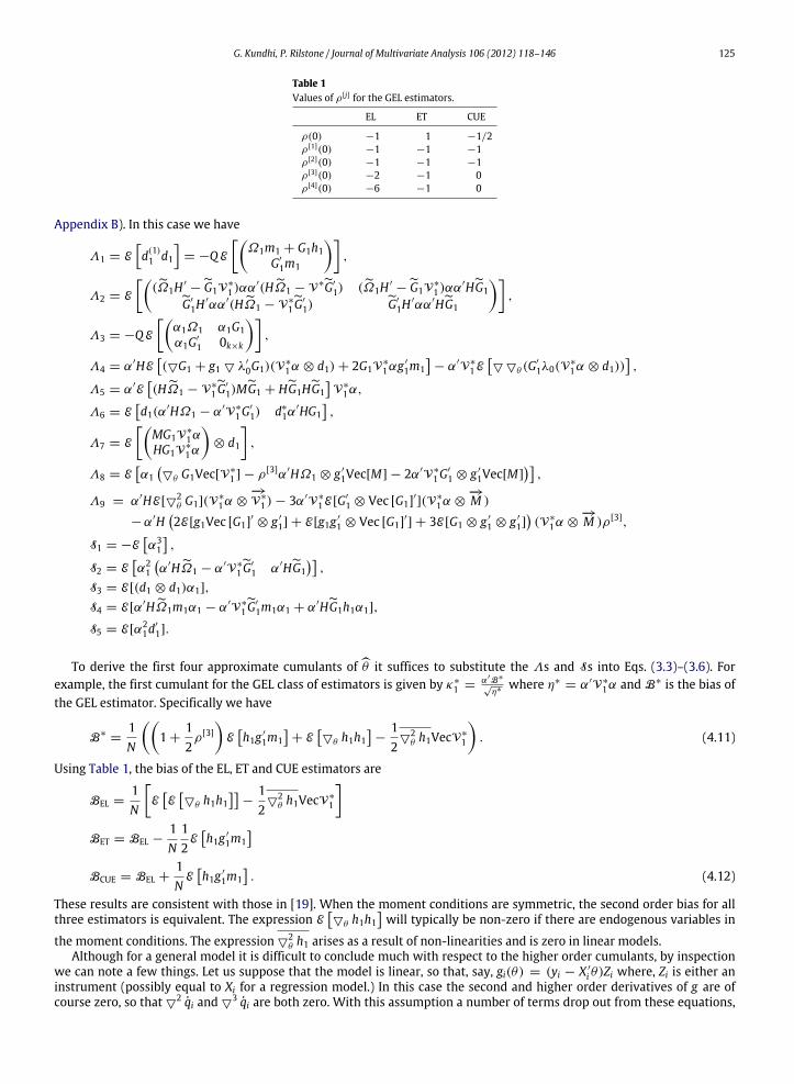
ρ(0) −1 1 −1/2ρ[1](0) −1 −1 −1ρ[2](0) −1 −1 −1ρ[3](0) −2 −1 0ρ[4](0) −6 −1 0
Appendix B). In this case we have
Λ1 = Ed(1)1 d1
= −QE
Ω1m1 + G1h1
G′
1m1
,
Λ2 = E
(Ω1H ′
−G1V∗
1 )αα′(HΩ1 − V∗G′
1) (Ω1H ′−G1V
∗
1 )αα′HG1G′
1H′αα′(HΩ1 − V∗
1G′
1)G′
1H′αα′HG1
,
Λ3 = −QE
α1Ω1 α1G1α1G′
1 0k×k
,
Λ4 = α′HE(G1 + g1 λ′
0G1)(V∗
1α ⊗ d1) + 2G1V∗
1αg′
1m1− α′V∗
1E θ (G
′
1λ0(V∗
1α ⊗ d1)),
Λ5 = α′E(HΩ1 − V∗
1G′
1)MG1 + HG1HG1V∗
1α,
Λ6 = Ed1(α′HΩ1 − α′V∗
1G′
1) d∗
1α′HG1
,
Λ7 = E
MG1V
∗
1αHG1V
∗
1α
⊗ d1
,
Λ8 = Eα1θ G1Vec[V∗
1 ] − ρ[3]α′HΩ1 ⊗ g ′
1Vec[M] − 2α′V∗
1G′
1 ⊗ g ′
1Vec[M]
,
Λ9 = α′HE[2θ G1](V
∗
1α ⊗−→V∗
1 ) − 3α′V∗
1E[G′
1 ⊗ Vec [G1]′](V∗
1α ⊗−→M )
− α′H2E[g1Vec [G1]′ ⊗ g ′
1] + E[g1g ′
1 ⊗ Vec [G1]′] + 3E[G1 ⊗ g ′
1 ⊗ g ′
1](V∗
1α ⊗−→M )ρ[3],
S1 = −Eα31
,
S2 = Eα21
α′HΩ1 − α′V∗
1G′
1 α′HG1
,
S3 = E[(d1 ⊗ d1)α1],
S4 = E[α′HΩ1m1α1 − α′V∗
1G′
1m1α1 + α′HG1h1α1],
S5 = E[α21d
′
1].
To derive the first four approximate cumulants of θ it suffices to substitute the Λs and Ss into Eqs. (3.3)–(3.6). Forexample, the first cumulant for the GEL class of estimators is given by κ∗
1 =α′B∗
√η∗ where η∗
= α′V∗
1α and B∗ is the bias ofthe GEL estimator. Specifically we have
B∗=
1N
1 +
12ρ[3]
Eh1g ′
1m1+ E
θ h1h1
−
12
2θ h1VecV∗
1
. (4.11)
Using Table 1, the bias of the EL, ET and CUE estimators are
BEL =1N
EEθ h1h1
−
12
2θ h1VecV∗
1
BET = BEL −
1N
12
Eh1g ′
1m1
BCUE = BEL +1N
Eh1g ′
1m1. (4.12)
These results are consistent with those in [19]. When the moment conditions are symmetric, the second order bias for allthree estimators is equivalent. The expression E
θ h1h1
will typically be non-zero if there are endogenous variables in
the moment conditions. The expression 2θ h1 arises as a result of non-linearities and is zero in linear models.
Although for a general model it is difficult to conclude much with respect to the higher order cumulants, by inspectionwe can note a few things. Let us suppose that the model is linear, so that, say, gi(θ) = (yi − X ′
i θ)Zi where, Zi is either aninstrument (possibly equal to Xi for a regression model.) In this case the second and higher order derivatives of g are ofcourse zero, so that
2 qi and 3 qi are both zero. With this assumption a number of terms drop out from these equations,
126 G. Kundhi, P. Rilstone / Journal of Multivariate Analysis 106 (2012) 118–146
although the presence of higher moments is quite pronounced through the lower moments of g and G. In practice, the firstfour cumulants can easily be estimated by their sample analogs.
5. Illustration
We conducted the simulations with a few purposes in mind. First we wanted to illustrate the techniques in the paper.Second we wished to compare results with the other prevalent technique: the bootstrap. To illustrate the techniques in thepaper we use an example from [10]; a simplified version of an asset-pricing model. The moment conditions are given as
E [exp(µ − θ(Xi + Zi) + 3Zi) − 1]E [Zi (exp(µ − θ(Xi + Zi) + 3Zi) − 1)] (5.1)
where Xi and Zi are scalars. Xi is sampled independently from N(0, s2) where s = 0.2 or 0.4. Zi has a marginal normaldistribution N(0, s2) and is independent of Xi. The true value of the estimated parameter θ is assumed to be equal to 3 andµ is a normalization constant. For GEL estimation there is one parameter and two restrictions with
gi(θ) =
exp(µ − θ(Xi + Zi) + 3Zi) − 1
Zi (exp(µ − θ(Xi + Zi) + 3Zi) − 1)
(5.2)
Gi(θ) = −
(Xi + Zi) exp(µ − θ(Xi + Zi) + 3Zi)
(Xi + Zi)Zi exp(µ − θ(Xi + Zi) + 3Zi)
. (5.3)
For GEL we have the FOCs
1N
qi(β)ρ[1](λ′gi(θ)) = 0. (5.4)
Put U = exp(µ − θ(Xi + Zi) + 3Zi).
q(β) =
U − 1Zi(U − 1)
−λ1(Xi + Zi)U − λ2(Xi + Zi)ZiU
(5.5)
q′(β) =U − 1 Zi(U − 1) −λ1(Xi + Zi)U − λ2(Xi + Zi)ZiU
(5.6)
q(β) =
0 0 −(Xi + Zi)U0 0 −(Xi + Zi)ZiU
−(Xi + Zi)U −(Xi + Zi)ZiU −λ1(Xi + Zi)2U − λ2(Xi + Zi)2ZiU
(5.7)
q =
0 0 −(Xi + Zi)U0 0 −(Xi + Zi)ZiU
−(Xi + Zi)U −(Xi + Zi)ZiU 0
(5.8)
2 q′
=
0 0 00 0 00 0 −(Xi + Zi)2U0 0 00 0 00 0 −(Xi + Zi)2ZiU0 0 (Xi + Zi)2U0 0 (Xi + Zi)2ZiU
(Xi + Zi)2U (Xi + Zi)2ZiU 0
(5.9)
q(1)i (β) = ((q)) ρ[1]
+q ⊗ q′
ρ[2]
=
0 0 −(Xi + Zi)U0 0 −(Xi + Zi)ZiU
−(Xi + Zi)U −(Xi + Zi)ZiU 0
(−1) +
g0
g ′ 0
(−1)
=
−gg ′
(Xi + Zi)U
(Xi + Zi)ZiU
(Xi + Zi)U (Xi + Zi)ZiU
0
(5.10)
q(1)i = −
(U − 1)2 (U − 1)2Zi −(Xi + Zi)UZi(U − 1)2 Z2
i (U − 1)2 −(Xi + Zi)ZiU−(Xi + Zi)U −(Xi + Zi)ZiU 0
(5.11)
G. Kundhi, P. Rilstone / Journal of Multivariate Analysis 106 (2012) 118–146 127
q(1)i = −
Ω −
E[(Xi + Zi)U]
E[(Xi + Zi)ZiU]
−E[(Xi + Zi)U] E[(Xi + Zi)ZiU]
0
(5.12)
where,
G = −
E[(Xi + Zi)U]
E[(Xi + Zi)ZiU]
, Ω =
E[(U − 1)2] E[(U − 1)2Zi]
E[Zi(U − 1)2] E[Z2i (U − 1)2]
. (5.13)
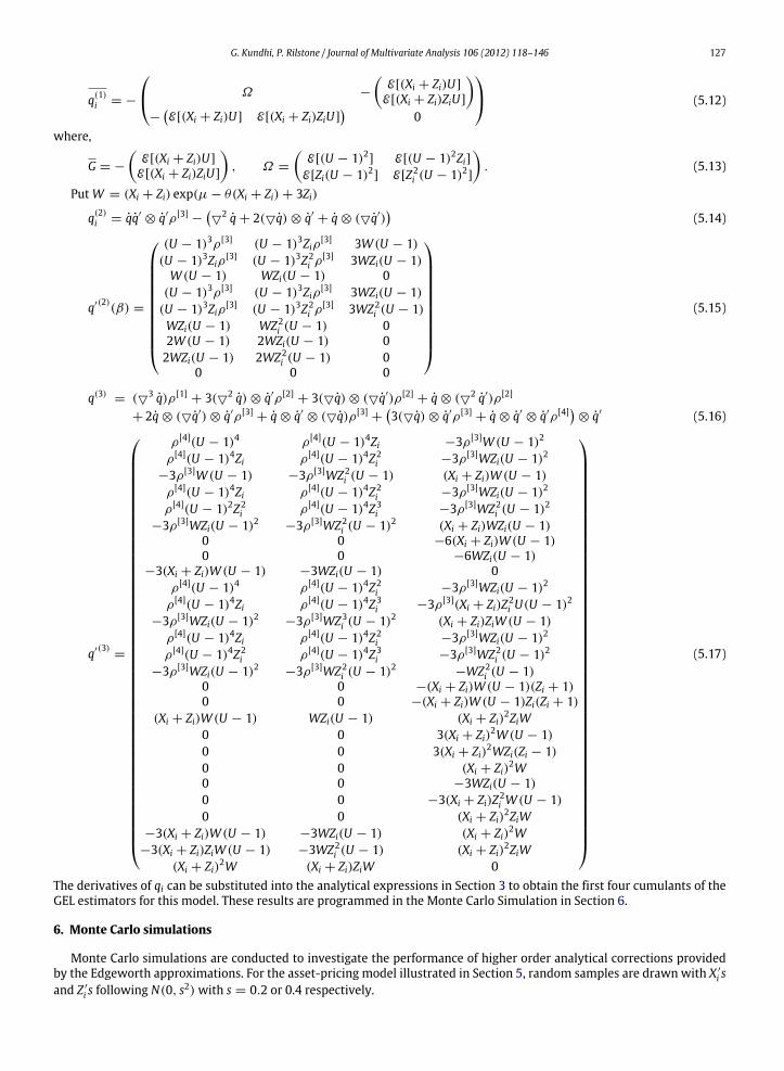
PutW = (Xi + Zi) exp(µ − θ(Xi + Zi) + 3Zi)
q(2)i = qq′
⊗ q′ρ[3]−
2 q + 2(q) ⊗ q′+ q ⊗ (q′)
(5.14)
q′(2)(β) =
(U − 1)3ρ[3] (U − 1)3Ziρ[3] 3W (U − 1)(U − 1)3Ziρ[3] (U − 1)3Z2
i ρ[3] 3WZi(U − 1)W (U − 1) WZi(U − 1) 0
(U − 1)3ρ[3] (U − 1)3Ziρ[3] 3WZi(U − 1)(U − 1)3Ziρ[3] (U − 1)3Z2
i ρ[3] 3WZ2i (U − 1)
WZi(U − 1) WZ2i (U − 1) 0
2W (U − 1) 2WZi(U − 1) 02WZi(U − 1) 2WZ2
i (U − 1) 00 0 0
(5.15)
q(3)= (3 q)ρ[1]
+ 3(2 q) ⊗ q′ρ[2]+ 3(q) ⊗ (q′)ρ[2]
+ q ⊗ (2 q′)ρ[2]
+ 2q ⊗ (q′) ⊗ q′ρ[3]+ q ⊗ q′
⊗ (q)ρ[3]+3(q) ⊗ q′ρ[3]
+ q ⊗ q′⊗ q′ρ[4]
⊗ q′ (5.16)
q′(3)=
ρ[4](U − 1)4 ρ[4](U − 1)4Zi −3ρ[3]W (U − 1)2
ρ[4](U − 1)4Zi ρ[4](U − 1)4Z2i −3ρ[3]WZi(U − 1)2
−3ρ[3]W (U − 1) −3ρ[3]WZ2i (U − 1) (Xi + Zi)W (U − 1)
ρ[4](U − 1)4Zi ρ[4](U − 1)4Z2i −3ρ[3]WZi(U − 1)2
ρ[4](U − 1)2Z2i ρ[4](U − 1)4Z3
i −3ρ[3]WZ2i (U − 1)2
−3ρ[3]WZi(U − 1)2 −3ρ[3]WZ2i (U − 1)2 (Xi + Zi)WZi(U − 1)
0 0 −6(Xi + Zi)W (U − 1)0 0 −6WZi(U − 1)
−3(Xi + Zi)W (U − 1) −3WZi(U − 1) 0ρ[4](U − 1)4 ρ[4](U − 1)4Z2
i −3ρ[3]WZi(U − 1)2
ρ[4](U − 1)4Zi ρ[4](U − 1)4Z3i −3ρ[3](Xi + Zi)Z2
i U(U − 1)2
−3ρ[3]WZi(U − 1)2 −3ρ[3]WZ3i (U − 1)2 (Xi + Zi)ZiW (U − 1)
ρ[4](U − 1)4Zi ρ[4](U − 1)4Z2i −3ρ[3]WZi(U − 1)2
ρ[4](U − 1)4Z2i ρ[4](U − 1)4Z3
i −3ρ[3]WZ2i (U − 1)2
−3ρ[3]WZi(U − 1)2 −3ρ[3]WZ2i (U − 1)2 −WZ2
i (U − 1)0 0 −(Xi + Zi)W (U − 1)(Zi + 1)0 0 −(Xi + Zi)W (U − 1)Zi(Zi + 1)
(Xi + Zi)W (U − 1) WZi(U − 1) (Xi + Zi)2ZiW0 0 3(Xi + Zi)2W (U − 1)0 0 3(Xi + Zi)2WZi(Zi − 1)0 0 (Xi + Zi)2W0 0 −3WZi(U − 1)0 0 −3(Xi + Zi)Z2
i W (U − 1)0 0 (Xi + Zi)2ZiW
−3(Xi + Zi)W (U − 1) −3WZi(U − 1) (Xi + Zi)2W−3(Xi + Zi)ZiW (U − 1) −3WZ2
i (U − 1) (Xi + Zi)2ZiW(Xi + Zi)2W (Xi + Zi)ZiW 0
(5.17)
The derivatives of qi can be substituted into the analytical expressions in Section 3 to obtain the first four cumulants of theGEL estimators for this model. These results are programmed in the Monte Carlo Simulation in Section 6.
6. Monte Carlo simulations
Monte Carlo simulations are conducted to investigate the performance of higher order analytical corrections providedby the Edgeworth approximations. For the asset-pricing model illustrated in Section 5, random samples are drawn with X ′
i sand Z ′
i s following N(0, s2) with s = 0.2 or 0.4 respectively.
128 G. Kundhi, P. Rilstone / Journal of Multivariate Analysis 106 (2012) 118–146
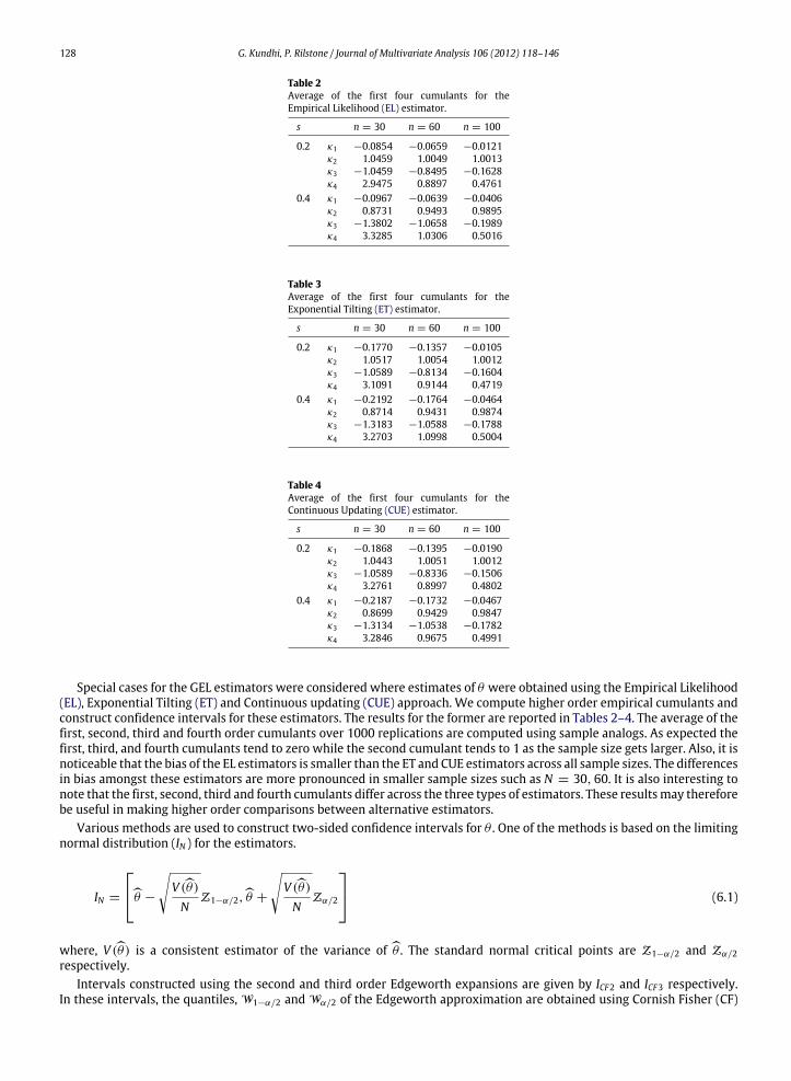
Table 2Average of the first four cumulants for theEmpirical Likelihood (EL) estimator.
s n = 30 n = 60 n = 100
0.2 κ1 −0.0854 −0.0659 −0.0121κ2 1.0459 1.0049 1.0013κ3 −1.0459 −0.8495 −0.1628κ4 2.9475 0.8897 0.4761
0.4 κ1 −0.0967 −0.0639 −0.0406κ2 0.8731 0.9493 0.9895κ3 −1.3802 −1.0658 −0.1989κ4 3.3285 1.0306 0.5016
Table 3Average of the first four cumulants for theExponential Tilting (ET) estimator.
s n = 30 n = 60 n = 100
0.2 κ1 −0.1770 −0.1357 −0.0105κ2 1.0517 1.0054 1.0012κ3 −1.0589 −0.8134 −0.1604κ4 3.1091 0.9144 0.4719
0.4 κ1 −0.2192 −0.1764 −0.0464κ2 0.8714 0.9431 0.9874κ3 −1.3183 −1.0588 −0.1788κ4 3.2703 1.0998 0.5004
Table 4Average of the first four cumulants for theContinuous Updating (CUE) estimator.
s n = 30 n = 60 n = 100
0.2 κ1 −0.1868 −0.1395 −0.0190κ2 1.0443 1.0051 1.0012κ3 −1.0589 −0.8336 −0.1506κ4 3.2761 0.8997 0.4802
0.4 κ1 −0.2187 −0.1732 −0.0467κ2 0.8699 0.9429 0.9847κ3 −1.3134 −1.0538 −0.1782κ4 3.2846 0.9675 0.4991
Special cases for the GEL estimators were considered where estimates of θ were obtained using the Empirical Likelihood(EL), Exponential Tilting (ET) and Continuous updating (CUE) approach. We compute higher order empirical cumulants andconstruct confidence intervals for these estimators. The results for the former are reported in Tables 2–4. The average of thefirst, second, third and fourth order cumulants over 1000 replications are computed using sample analogs. As expected thefirst, third, and fourth cumulants tend to zero while the second cumulant tends to 1 as the sample size gets larger. Also, it isnoticeable that the bias of the EL estimators is smaller than the ET and CUE estimators across all sample sizes. The differencesin bias amongst these estimators are more pronounced in smaller sample sizes such as N = 30, 60. It is also interesting tonote that the first, second, third and fourth cumulants differ across the three types of estimators. These resultsmay thereforebe useful in making higher order comparisons between alternative estimators.
Various methods are used to construct two-sided confidence intervals for θ . One of the methods is based on the limitingnormal distribution (IN ) for the estimators.
IN =
θ −
V (θ)
NZ1−α/2,θ +
V (θ)
NZα/2
(6.1)
where, V (θ) is a consistent estimator of the variance of θ . The standard normal critical points are Z1−α/2 and Zα/2respectively.
Intervals constructed using the second and third order Edgeworth expansions are given by ICF2 and ICF3 respectively.In these intervals, the quantiles, W1−α/2 and Wα/2 of the Edgeworth approximation are obtained using Cornish Fisher (CF)

G. Kundhi, P. Rilstone / Journal of Multivariate Analysis 106 (2012) 118–146 129
Table 5Confidence intervals for Empirical Likelihood (EL) estimator: average length (Avl) and coverage probabilities (Cov) at 90%, 95% and 99% levels.
s 90 90 95 95 99 99Avl Cov Avl Cov Avl Cov
n = 30
0.2 IN 3.1745 0.8690 3.7939 0.9180 4.9941 0.9570ICF2 3.2939 0.8820 3.8935 0.9360 5.5476 0.9780ICF3 3.4788 0.9060 4.5407 0.9590 6.3832 0.9960IBD 2.8859 0.8580 3.9955 0.9030 5.6238 0.9410IBt 2.8747 0.8850 4.0584 0.9350 6.2361 0.9730
0.4 IN 2.8450 0.8600 3.6480 0.9100 4.7404 0.9520ICF2 2.8618 0.8790 3.8848 0.9390 4.8842 0.9790ICF3 3.1629 0.9090 4.2732 0.9540 6.3418 0.9900IBD 2.8748 0.8560 3.8106 0.9040 4.9041 0.9490IBt 3.1734 0.8820 4.2114 0.9360 5.1752 0.9760
n = 60
0.2 IN 2.2156 0.8780 2.6478 0.9340 3.4854 0.9630ICF2 2.2291 0.8900 2.6814 0.9410 3.7463 0.9870ICF3 2.3438 0.9010 2.9477 0.9540 4.4084 0.9910IBD 2.3653 0.8620 2.7015 0.9260 3.9338 0.9550IBt 2.4396 0.8940 3.1821 0.9420 4.1655 0.9820
0.4 IN 2.2714 0.8790 2.7146 0.9310 3.5733 0.9660ICF2 2.2852 0.8890 2.7946 0.9380 3.8750 0.9880ICF3 2.4821 0.9060 3.2286 0.9520 4.5092 0.9930IBD 2.1409 0.8600 3.1367 0.9260 4.2851 0.9590IBt 2.3209 0.8910 3.1733 0.9410 4.4362 0.9820
n = 100
0.2 IN 1.7119 0.8930 2.2460 0.9360 2.6932 0.9790ICF2 1.7224 0.8950 2.2692 0.9470 2.8932 0.9860ICF3 1.7791 0.9060 2.3940 0.9520 2.9669 0.9980IBD 1.7122 0.8840 2.3654 0.9340 2.8556 0.9770IBt 1.8625 0.8970 2.2646 0.9460 3.0886 0.9800
0.4 IN 1.8625 0.8880 2.2527 0.9410 2.7756 0.9820ICF2 1.9030 0.9010 2.2720 0.9540 2.9297 0.9910ICF3 1.9858 0.9050 2.3944 0.9550 3.0865 0.9950IBD 1.8254 0.8770 2.3469 0.9370 2.9164 0.9760IBt 1.8789 0.9030 2.2700 0.9450 2.8102 0.9850
expansions given in Section 3.
ICF =
θ −
V
NW1−α/2,θ +
V
NWα/2
. (6.2)
The second order Cornish Fisher expansion (i.e., terms up to order O(N−1)) corrects the standard normal interval for bias,dispersion and skewness. While the third order Cornish Fisher expansion (i.e., terms up to order O(N−3/2)) provides finitesample corrections for kurtosis and a secondary effect of skewness.
Two types of bootstrap confidence intervals are also constructed; the bootstrap percentile and percentile-t . The numberof bootstrap resamples drawn in each replication of 1000 simulations is set to 999. Davidson and MacKinnon [7] provide adiscussion on choosing thenumber of bootstrap resamples. The bootstrappercentile interval is constructedusingBbootstrapestimates θ∗
i with nonparametric bootstrap resamples. The (1−α)100% empirical quantiles were obtained by sorting theseestimates. The two-sided bootstrap percentile confidence interval, IBD is defined as
IBD =
θ∗(1−α/2)
, θ∗(α/2)
. (6.3)
Although the bootstrap percentile interval is simpler to construct, it is in general a non-pivotal method typically having aninferior coverage accuracy in practice.
The percentile t-interval is constructed using a bootstrap t-statistic. This is asymptotically pivotal and given by
t∗ =
θ∗ −θσ θ∗ (6.4)
where σ θ∗is the standard error of the bootstrap estimates. The (1 − α)100% quantiles of the distribution of the
bootstrap t-statistic were obtained. These are used as critical points in the construction of the two-sided bootstrap

130 G. Kundhi, P. Rilstone / Journal of Multivariate Analysis 106 (2012) 118–146
Table 6Confidence intervals for Exponential Tilting (ET) estimator: average length (Avl) and coverage probabilities (Cov) at 90%, 95% and 99% levels.
s 90 90 95 95 99 99Avl Cov Avl Cov Avl Cov
n = 30
0.2 IN 3.1875 0.8680 3.8095 0.9140 5.0145 0.9580ICF2 3.2070 0.8830 3.8471 0.9350 5.5086 0.9760ICF3 3.5221 0.9090 4.6334 0.9450 6.5431 0.9860IBD 2.7131 0.8590 3.8713 0.9040 5.5493 0.9470IBt 2.9228 0.8810 3.9758 0.9330 5.9029 0.9790
0.4 IN 2.8450 0.8660 3.6806 0.9120 4.6184 0.9430ICF2 2.8618 0.8860 3.8640 0.9380 4.8404 0.9750ICF3 3.1413 0.9050 4.2672 0.9470 6.1338 0.9810IBD 2.8037 0.8570 3.7313 0.9060 5.1090 0.9450IBt 3.3378 0.8870 3.9973 0.9360 5.2560 0.9710
n = 60
0.2 IN 2.2100 0.8750 2.6413 0.9350 3.4768 0.9610ICF2 2.2235 0.8960 2.6685 0.9430 3.7677 0.9800ICF3 2.3368 0.9050 2.9372 0.9540 4.0250 0.9880IBD 2.5308 0.8640 2.6040 0.9240 3.9254 0.9590IBt 2.4420 0.8920 3.1201 0.9420 4.0873 0.9820
0.4 IN 2.2717 0.8770 2.7150 0.9270 3.5738 0.9660ICF2 2.2856 0.8890 2.7992 0.9450 3.7382 0.9830ICF3 2.4825 0.9090 3.2254 0.9500 4.5097 0.9930IBD 2.1384 0.8660 3.2187 0.9280 4.5029 0.9570IBt 2.5045 0.8910 3.1478 0.9470 4.6437 0.9780
n = 100
0.2 IN 1.7037 0.8960 2.2361 0.9390 2.6802 0.9750ICF2 1.7141 0.9050 2.2640 0.9470 2.8225 0.9820ICF3 1.7709 0.9080 2.3843 0.9490 2.9541 0.9870IBD 1.7268 0.8840 2.3738 0.9320 2.8593 0.9720IBt 1.8031 0.8980 2.3898 0.9450 2.8584 0.9920
0.4 IN 1.8970 0.8870 2.2056 0.9380 2.7983 0.9730ICF2 1.9094 0.8900 2.2564 0.9490 2.8272 0.9870ICF3 1.9336 0.9040 2.4274 0.9510 2.8871 0.9950IBD 1.8666 0.8700 2.3800 0.9340 2.6001 0.9780IBt 2.0144 0.9040 2.3703 0.9480 2.8285 0.9880
percentile t-interval, IBt . The two-sided equal-tailed percentile t-interval is given as
IBt =
θ +σ(θ)t∗(1−α/2),θ +σ(θ)t∗(α/2)
. (6.5)
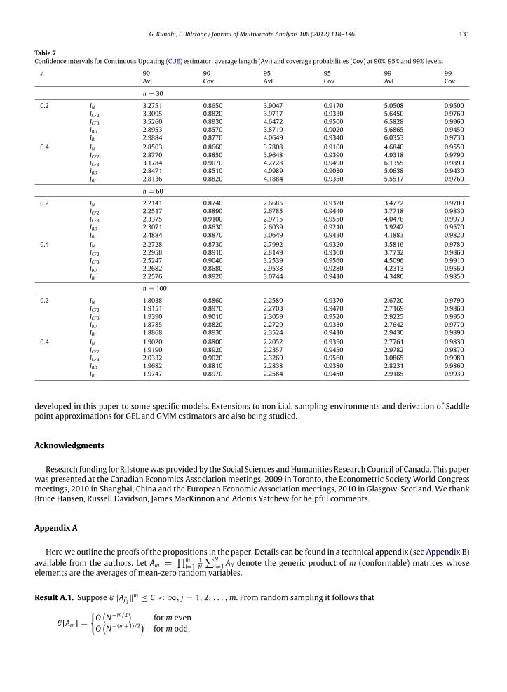
The average length (Avl) and coverage probability (Cov) of confidence intervals are computed in this experiment. Resultswhere θ is estimated using the Empirical Likelihood, Exponential Tilting and CUE methods are reported in Tables 5–7respectively. The bootstrap percentile interval performs poorly with higher coverage errors in comparison to all the otherintervals. This is especially so for sample sizes 30 and 60. The coverage accuracy of the percentile t-intervals is relativelyhigher than the bootstrap percentile interval. However, for smaller samples the coverage of percentile t-interval is belowthe nominal at all levels. The standard normal interval for all three estimators yields inferior coverage especially in smallersamples N = 30, 60. The second order CF correction to the standard normal interval improves the coverage. A thirdorder CF correction further reduces coverage errors and works well in improving coverage accuracy of the intervals. Thisimprovement is especially noticeable in smaller samples at the 90%, 95% and 99% level and for all three estimators. Thesecond and third order analytical corrections using Edgeworth approximations therefore seem to improve coverage ofconfidence intervals, especially for smaller samples.
7. Conclusion
This paper derives Edgeworth expansions for GEL estimators. The results obtained are also applicable to a wide classof estimators including GMM. The methods are simple to implement using most computer packages which have someprogramming capability. The simulation results for confidence interval construction indicate that higher order analyticalcorrections work well compared to first-order approximations and improve inferences in smaller samples. The authorsare currently working on derivation of Edgeworth expansions for GMM estimators and the application of the technique
G. Kundhi, P. Rilstone / Journal of Multivariate Analysis 106 (2012) 118–146 131
Table 7Confidence intervals for Continuous Updating (CUE) estimator: average length (Avl) and coverage probabilities (Cov) at 90%, 95% and 99% levels.
s 90 90 95 95 99 99Avl Cov Avl Cov Avl Cov
n = 30
0.2 IN 3.2751 0.8650 3.9047 0.9170 5.0508 0.9500ICF2 3.3095 0.8820 3.9717 0.9330 5.6450 0.9760ICF3 3.5260 0.8930 4.6472 0.9500 6.5828 0.9960IBD 2.8953 0.8570 3.8719 0.9020 5.6865 0.9450IBt 2.9884 0.8770 4.0649 0.9340 6.0353 0.9730
0.4 IN 2.8503 0.8660 3.7808 0.9100 4.6840 0.9550ICF2 2.8770 0.8850 3.9648 0.9390 4.9318 0.9790ICF3 3.1784 0.9070 4.2728 0.9490 6.1355 0.9890IBD 2.8471 0.8510 4.0989 0.9030 5.0638 0.9430IBt 2.8136 0.8820 4.1884 0.9350 5.5517 0.9760
n = 60
0.2 IN 2.2141 0.8740 2.6685 0.9320 3.4772 0.9700ICF2 2.2517 0.8890 2.6785 0.9440 3.7718 0.9830ICF3 2.3375 0.9100 2.9715 0.9550 4.0476 0.9970IBD 2.3071 0.8630 2.6039 0.9210 3.9242 0.9570IBt 2.4884 0.8870 3.0649 0.9430 4.1883 0.9820
0.4 IN 2.2728 0.8730 2.7992 0.9320 3.5816 0.9780ICF2 2.2958 0.8910 2.8149 0.9360 3.7732 0.9860ICF3 2.5247 0.9040 3.2539 0.9560 4.5096 0.9910IBD 2.2682 0.8680 2.9538 0.9280 4.2313 0.9560IBt 2.2576 0.8920 3.0744 0.9410 4.3480 0.9850
n = 100
0.2 IN 1.8038 0.8860 2.2580 0.9370 2.6720 0.9790ICF2 1.9151 0.8970 2.2703 0.9470 2.7169 0.9860ICF3 1.9390 0.9010 2.3059 0.9520 2.9225 0.9950IBD 1.8785 0.8820 2.2729 0.9330 2.7642 0.9770IBt 1.8868 0.8930 2.3524 0.9410 2.9430 0.9890
0.4 IN 1.9020 0.8800 2.2052 0.9390 2.7761 0.9830ICF2 1.9190 0.8920 2.2357 0.9450 2.9782 0.9870ICF3 2.0332 0.9020 2.3269 0.9560 3.0865 0.9980IBD 1.9682 0.8810 2.2838 0.9380 2.8231 0.9860IBt 1.9747 0.8970 2.2584 0.9450 2.9185 0.9930
developed in this paper to some specific models. Extensions to non i.i.d. sampling environments and derivation of Saddlepoint approximations for GEL and GMM estimators are also being studied.
Acknowledgments
Research funding for Rilstonewas provided by the Social Sciences andHumanities Research Council of Canada. This paperwas presented at the Canadian Economics Association meetings, 2009 in Toronto, the Econometric Society World Congressmeetings, 2010 in Shanghai, China and the European Economic Association meetings, 2010 in Glasgow, Scotland. We thankBruce Hansen, Russell Davidson, James MacKinnon and Adonis Yatchew for helpful comments.
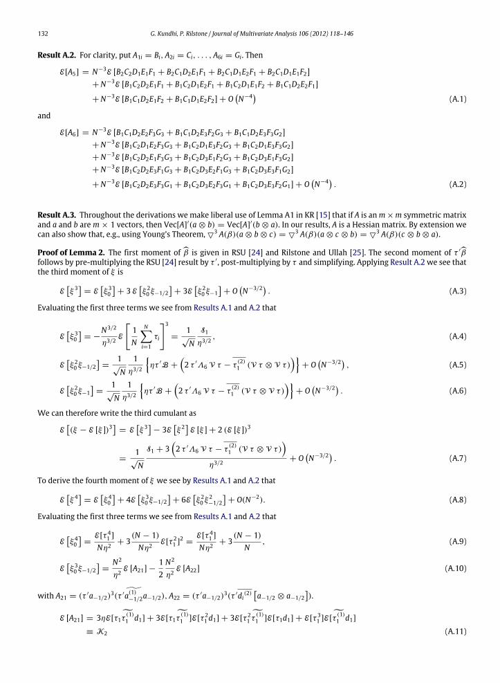
Appendix A
Herewe outline the proofs of the propositions in the paper. Details can be found in a technical appendix (see Appendix B)available from the authors. Let Am =
ml=1
1N
Ni=1 Ali denote the generic product of m (conformable) matrices whose
elements are the averages of mean-zero random variables.
Result A.1. Suppose E∥Ajij∥m
≤ C < ∞, j = 1, 2, . . . ,m. From random sampling it follows that
E[Am] =
ON−m/2 form even
ON−(m+1)/2 form odd.
132 G. Kundhi, P. Rilstone / Journal of Multivariate Analysis 106 (2012) 118–146
Result A.2. For clarity, put A1i = Bi, A2i = Ci, . . . , A6i = Gi. Then
E[A5] = N−3E [B2C2D1E1F1 + B2C1D2E1F1 + B2C1D1E2F1 + B2C1D1E1F2]+N−3E [B1C2D2E1F1 + B1C2D1E2F1 + B1C2D1E1F2 + B1C1D2E2F1]
+N−3E [B1C1D2E1F2 + B1C1D1E2F2] + ON−4 (A.1)
and
E[A6] = N−3E [B1C1D2E2F3G3 + B1C1D2E3F2G3 + B1C1D2E3F3G2]+N−3E [B1C2D1E2F3G3 + B1C2D1E3F2G3 + B1C2D1E3F3G2]+N−3E [B1C2D2E1F3G3 + B1C2D3E1F2G3 + B1C2D3E1F3G2]+N−3E [B1C2D2E3F1G3 + B1C2D3E2F1G3 + B1C2D3E3F1G2]
+N−3E [B1C2D2E3F3G1 + B1C2D3E2F3G1 + B1C2D3E3F2G1] + ON−4 . (A.2)
Result A.3. Throughout the derivations wemake liberal use of Lemma A1 in KR [15] that if A is anm×m symmetric matrixand a and b are m × 1 vectors, then Vec[A]
′(a ⊗ b) = Vec[A]′(b ⊗ a). In our results, A is a Hessian matrix. By extension we
can also show that, e.g., using Young’s Theorem, 3 A(β)(a ⊗ b ⊗ c) = 3 A(β)(a ⊗ c ⊗ b) =
3 A(β)(c ⊗ b ⊗ a).
Proof of Lemma 2. The first moment of β is given in RSU [24] and Rilstone and Ullah [25]. The second moment of τ ′βfollows by pre-multiplying the RSU [24] result by τ ′, post-multiplying by τ and simplifying. Applying Result A.2 we see thatthe third moment of ξ is
Eξ 3
= Eξ 30
+ 3 E
ξ 20 ξ−1/2
+ 3E
ξ 20 ξ−1
+ O
N−3/2 . (A.3)
Evaluating the first three terms we see from Results A.1 and A.2 that
Eξ 30
= −
N3/2
η3/2E
1N
Ni=1
τi
3
=1
√N
S1
η3/2, (A.4)
Eξ 20 ξ−1/2
=
1√N
1η3/2
ητ ′B +
2 τ ′Λ6 V τ − τ
(2)1 (V τ ⊗ V τ)
+ O
N−3/2 , (A.5)
Eξ 20 ξ−1
=
1√N
1η3/2
ητ ′B +
2 τ ′Λ6 V τ − τ
(2)1 (V τ ⊗ V τ)
+ O
N−3/2 . (A.6)
We can therefore write the third cumulant as
E(ξ − E [ξ ])3
= E
ξ 3
− 3Eξ 2 E [ξ ] + 2 (E [ξ ])3
=1
√N
S1 + 32 τ ′Λ6 V τ − τ
(2)1 (V τ ⊗ V τ)
η3/2
+ ON−3/2 . (A.7)
To derive the fourth moment of ξ we see by Results A.1 and A.2 that
Eξ 4
= Eξ 40
+ 4E
ξ 30 ξ−1/2
+ 6E
ξ 20 ξ 2
−1/2
+ O(N−2). (A.8)
Evaluating the first three terms we see from Results A.1 and A.2 that
Eξ 40
=
E[τ 41 ]
Nη2+ 3
(N − 1)Nη2
E[τ 21 ]
2=
E[τ 41 ]
Nη2+ 3
(N − 1)N
, (A.9)
Eξ 30 ξ−1/2
=
N2
η2E [A21] −
12N2
η2E [A22] (A.10)
with A21 = (τ ′a−1/2)3(τ ′ a(1)
−1/2a−1/2), A22 = (τ ′a−1/2)3(τ ′di(2)
a−1/2 ⊗ a−1/2
).
E [A21] = 3ηE[τ1τ
(1)1 d1] + 3E[τ1
τ
(1)1 ]E[τ 2
1 d1] + 3E[τ 21τ
(1)1 ]E[τ1d1] + E[τ 3
1 ]E[τ
(1)1 d1]
≡ K2 (A.11)
G. Kundhi, P. Rilstone / Journal of Multivariate Analysis 106 (2012) 118–146 133
and
E [A22] = 3ηE[τ1τ1(2)(d1 ⊗ d1)] + 3τi(2)(E[τ1d1] ⊗ E[τ 21 d1])
+ 3τ1(2)(E[τ 21 d1] ⊗ E[τ1d1]) + E[τ 3
1 ]τi(2)(E[d1 ⊗ d1])≡ K3. (A.12)
Eξ 20 ξ 2
−1/2
=
N2
η2E
A61 +
14A62 − A63
(A.13)
with A41 = (τ ′a−1/2)2(τ ′ a(1)
−1/2a−1/2)2, A42 = (τ ′a−1/2)
2(τ ′di(2)a−1/2 ⊗ a−1/2
)2, A43 = (τ ′a−1/2)
2(τ ′ a(1)−1/2
a−1/2)(τ′di(2)
a−1/2 ⊗ a−1/2
). From Results A.1 and A.2 we have:
N3E[A41] = η
(τ ′Λ1)
2+τ
(1)2 Vτ
(1)2
′
+ τ(1)2 Λ6d2
+ O
N−1
+ 22Trace[τ ′Λ6Vτ ′(τ ′Λ1)] + τ ′Λ6VΛ′
6τ + 2τ ′Λ6Λ6Vτ ′+ τVτ
(1)3τ
(1)3 Vτ ′
≡ K4 + O
N−1 , (A.14)
N3E[A42] = ητ(2)1
−→V1
−→V1
′
+ 2(V ⊗ V)τ
(2)1
′
+ 2τ (2)1
(Vτ ⊗ Vτ)
−→V1
′
+ 2(VτVτ ′⊗ V)
τ
(2)1
′
+ 2τ (2)1
2V ⊗ Vττ ′V +
−→V1(τ
′V ⊗ τ ′V)τ
(2)1
′
+ ON−1
≡ K5 + ON−1 , (A.15)
N3E[A43] = η(τ ′Λ1)
−→V1
′
+ 2d′
2 ⊗ τ(1)2 V
τ1(2)
′
+ 4τ ′V ⊗ τ ′Λ6V + τ ′V ⊗ d′
3τ(1)3 τ ′V
τ1(2)
′
+ 2τ ′Λ6Vτ
−→V1
′
+ (τ ′Λ1)τ′V ⊗ τ ′V
τ1(2)
′
+ ON−1
≡ K6 + ON−1 . (A.16)
Put
Ξ = 4
1η2
K1 −1
2η2K2
+ 6
1η2
K4 −1
4η2K5 −
1η2
K6
. (A.17)
We can write the fourth cumulant of ξ, κ∗
4 ≡ E(ξ − E [ξ ])4
− 3(Var[ξ ])2 as
κ∗
4 = Eξ 4
− 4Eξ 3 E [ξ ] − 3
Eξ 22
+ 12Eξ 2 (E [ξ ])2 − 6E [ξ ]4
=Eτ 4i
− 3η2
η2N+
Ξ
N− 6
Π
N− 4
τ ′B
N
S1 + 3
2 τ ′Λ6 V τ − τ
(2)1 (V τ ⊗ V τ)
η2
+ ON−2 . (A.18)
Proof of Proposition 3. The characteristic function of ξ ∗= ξ − κ1/
√N can be written
χ(t) = e−t2/21 −
16(−it)3
κ3√N
+36Π(−it)2 + 3κ4(−it)4 + κ2
3 (−it)6
72N
+ o
N−1 . (A.19)
Define Hermite polynomials as H1(z) = z,H2(z) = z2 − 1,H3(z) = z3 − 3z,H5(z) = z5 − 10z3 + 15z. Using standardresults we have
Pr(ξ ∗≤ z) = Φ(z) −
16
κ3√NH2(z) +
36ΠH1(z) + 3κ4H3(z) + κ23H5(z)
72N
φ(z) + o
N−1 . (A.20)
Appendix B. Technical Appendix to accompany [15]
This appendix provides some of the details to the proofs of the propositions in the paper which derive the Edgeworthexpansions. Throughout this appendixwe let Am =
ml=1
1N
Ni=1 Ali denote the generic product ofm (conformable)matrices
whose elements are the averages of mean-zero random variables.
134 G. Kundhi, P. Rilstone / Journal of Multivariate Analysis 106 (2012) 118–146
Result B.1. Suppose E∥Ajij∥m
≤ C < ∞, j = 1, 2, . . . ,m. Then
E[Am] =
ON−m/2 form even
ON−(m+1)/2 form odd.
Proof. Supposem > 1; otherwise E [Am] = 0.
E [Am] = E
ml=1
1N
Ni=1
Ali
= N−mN
i1=1
Ni2=1
· · ·
Nim=1
EA1i1A2i2 · · · Amim
. (B.1)
The summands can be non-zero only if two or more of the ij indices are the same. There are various permutations when thiscan happen. Supposem is even. With respect to order of magnitude the most numerous terms will correspond to situationswhen there are m/2 pairs of Ajij with common subscript ijs. This can happen in the order of Nm/2 times. With m odd themost numerous terms will correspond to situations when there are (m − 3)/2 pairs of Ajij with common subscript ijs andone triplet of Ajij with common subscript ijs. This can happen in the order of N (m−1)/2 times. We thus have
E[Am] =
N−mO
Nm/2
= ON−m/2 form even
N−mON (m−1)/2
= ON−(m+1)/2 form odd.
(B.2)
Result B.2. For clarity, put A1i = Bi, A2i = Ci, . . . , A6i = Gi. Then
E[A5] = N−3E [B2C2D1E1F1 + B2C1D2E1F1 + B2C1D1E2F1 + B2C1D1E1F2]+N−3E [B1C2D2E1F1 + B1C2D1E2F1 + B1C2D1E1F2 + B1C1D2E2F1]
+N−3E [B1C1D2E1F2 + B1C1D1E2F2] + ON−4 (B.3)
and
E[A6] = N−3E [B1C1D2E2F3G3 + B1C1D2E3F2G3 + B1C1D2E3F3G2]+N−3E [B1C2D1E2F3G3 + B1C2D1E3F2G3 + B1C2D1E3F3G2]+N−3E [B1C2D2E1F3G3 + B1C2D3E1F2G3 + B1C2D3E1F3G2]+N−3E [B1C2D2E3F1G3 + B1C2D3E2F1G3 + B1C2D3E3F1G2]
+N−3E [B1C2D2E3F3G1 + B1C2D3E2F3G1 + B1C2D3E3F2G1] + ON−4 . (B.4)
Proof. The expectation of the summands in Am are zero if one or more of the ij subscripts is unique. Form = 5 we have
E [A5] = N−5N
i1=1
Ni2=1
· · ·
Ni5=1
EBi1Ci2 · · · Fi5
. (B.5)
There are two situations where the summands are not zero. One is if all the subscripts are the same. This only occurs Ntimes. The other cases are when two of the indices are the same and are different from the other three which are also thesame. Each of these combinations can occur N(N − 1) the result follows.
For m = 6 we have
E [A6] = N−6N
i1=1
Ni2=1
· · ·
Ni6=1
EBi1Ci2 · · ·Gi6
. (B.6)
There are four situations where the summands are not zero. One is if all the subscripts are the same. This only occurs Ntimes. The second case is when three of the indices are the same and are different from the other three which are also thesame. Each of these combinations can occur N(N − 1) times. The third case is when two of the indices are the same and aredifferent from the other four which are also the same. Each of these combinations can occur N(N − 1) times. The other setof cases is when there are three sets of like subscripts, but the index within each set is different from that in the other twogroups. Each of these combinations can occur N(N − 1)(N − 2) times.
G. Kundhi, P. Rilstone / Journal of Multivariate Analysis 106 (2012) 118–146 135
Result B.3. Throughout the derivations we make liberal use of Lemma A1 in KR [15] that if A is anm×m symmetric matrixand a and b are m × 1 vectors, then Vec[A]
′(a ⊗ b) = Vec[A]′(b ⊗ a). In our results, A is a Hessian matrix. By extension we
can also show that, e.g., using Young’ Theorem, 3 A(β)(a ⊗ b ⊗ c) = 3 A(β)(a ⊗ c ⊗ b).
Proof to Lemma 2. The second moment of β is given in RSU [24] and Rilstone and Ullah [25]. The second moment of βfollows by pre-multiplying that result by τ ′, post-multiplying by τ and simplifying. The third moment of ξ is
Eξ 3
= E
ξ0 + ξ−1/2 + ξ−13
= Eξ 30
+ 3E
ξ 20 ξ−1/2
+ TN (B.7)
where
TN ≡ Eξ 3−1/2 + ξ 3
−1 + 3ξ0ξ 2−1/2 + 3ξ0ξ 2
−1 + 3ξ−1ξ2−1/2 + 3ξ 2
0 ξ−1+ E
6ξ0ξ−1/2ξ−1 + 3ξ 2
−1ξ−1/2. (B.8)
Applying Result B.1 we see that TN is of the form and magnitude as follows
TN = N3/2E [A6 + A9 + A5 + A7 + A7 + A5 + A6 + A8]
= N3/2ON−3
= ON−3/2 (B.9)
so that
Eξ 3
= Eξ 30
+ 3E
ξ 20 ξ−1/2
+ 3E
ξ 20 ξ−1
+ O
N−3/2 . (B.10)
Evaluating the first two terms we see first that
Eξ 30
= E
N/θτ ′a−1/2
3
= −N3/2
η3/2E
1N
Ni=1
τi
3
= −N3/2
η3/2
1N3
NEτ 3i
=
1√N
S1
η3/2. (B.11)
From the random sampling assumption and Lemma A1
Eξ 20 ξ−1/2
=
1√N
1η3/2
E
τ1τ1
τ
(1)2 d2 −
12τ
(2)1 (d2 ⊗ d2)
+
1√N
1η3/2
E
τ1τ2
τ
(1)1 d2 −
12τ
(2)1 (d1 ⊗ d2)
+
1√N
1η3/2
E
τ1τ2
τ
(1)2 d1 −
12τ
(2)1 (d2 ⊗ d1)
+ O
N−3/2
=1
√N
1η3/2
ητ ′B +
2τ ′Λ6Vτ − τ
(2)1 (Vτ ⊗ Vτ)
+ O
N−3/2 (B.12)
and
Eξ 20 ξ−1
=
1√N
1η3/2
E
τ1τ1
τ
(1)2 d2 −
12τ
(2)1 (d2 ⊗ d2)
+
1√N
1η3/2
E
τ1τ2
τ
(1)1 d2 −
12τ
(2)1 (d1 ⊗ d2)
+
1√N
1η3/2
E
τ1τ2
τ
(1)2 d1 −
12τ
(2)1 (d2 ⊗ d1)
+ O
N−3/2
=1
√N
1η3/2
ητ ′B +
2τ ′Λ6Vτ − τ
(2)1 (Vτ ⊗ Vτ)
+ O
N−3/2 (B.13)
so that
Eξ 3
=1
√N
S1 + 3ητ ′B + S2
η3/2
+ ON−3/2 . (B.14)
136 G. Kundhi, P. Rilstone / Journal of Multivariate Analysis 106 (2012) 118–146
We can therefore write the third cumulant as
E(ξ − E [ξ ])3
= E
ξ 3
− 3Eξ 2 E [ξ ] + 2 (E [ξ ])3
=1
√N
S1 + 3ητ ′B +
2τ ′Λ6Vτ − τ
(2)1 (Vτ ⊗ Vτ)
η3/2
− 31
√N
τ ′B√
η+ O
N−3/2
=1
√N
S1 + 32τ ′Λ6Vτ − τ
(2)1 (Vτ ⊗ Vτ)
η3/2
+ ON−3/2 . (B.15)
The fourth moment of ξ is
Eξ 4
= E
ξ0 + ξ−1/2 + ξ−14
= Eξ 40
+ 4E
ξ 30 ξ−1/2
+ 6E
ξ 20 ξ 2
−1/2
+ TN (B.16)
where
TN ≡ E4ξ0ξ 3
−1/2 + ξ 4−1/2 + · · · + ξ 4
−1
. (B.17)
Consider the largest (in order) term on the right hand side of (A.16). It is of the form
Eξ0ξ
3−1/2
= N2E[A7] = O(N−2) (B.18)
where A7 is a polynomial of the form in Lemma A2 and the subscript ‘‘7’’ refers to its order. We see that
Eξ 40
=
E[τ 41 ]
Nη2+ 3
(N − 1)Nη2
E[τ 21 ]
2=
E[τ 41 ]
Nη2+ 3
(N − 1)N
. (B.19)
Next,
Eξ 30 ξ−1/2
=
N2
η2E(τ ′a−1/2)
3(τ ′a−1)
=N2
η2E
(τ ′a−1/2)
3(τ ′ a(1)−1/2a−1/2)
−
12N2
η2E(τ ′a−1/2)
3τ ′di(2)
a−1/2 ⊗ a−1/2
. (B.20)
Result B.2 can be applied to the first term of the right hand side of (B.19). By inspection of the result in (A.2) we see thereare 10 terms (apart from the O(N−4) term). From the scalarization induced by τ this simplifies to
E
(τ ′a−1/2)
3(τ ′ a(1)−1/2a−1/2)
= 3ηE[τ1
τ
(1)1 d1] + 3E[τ1
τ
(1)1 ]E[τ 2
1 d1] + 3E[τ 21τ
(1)1 ]E[τ1d1] + E[τ 3
1 ]E[τ
(1)1 d1]
= 3ηE[τ1τ
(1)1 d1] + 3CE[τ 2
1 d1] + 3E[τ 21τ
(1)1 ]E[τ1d1] − S1τ
′Λ1
≡ K2. (B.21)
Similarly, Result B.2 can be applied to the second term of the right hand side of (A.19). By inspection of the result in (A.2)we see there are 10 terms (apart from an O(N−4) term). So the second term (ST) can be written such that
ST = 3ηE[τ1τ1(2)(d1 ⊗ d1)] + 3τi(2)(E[τ1d1] ⊗ E[τ 21 d1]) + 3τ1(2)(E[τ 2
1 d1] ⊗ E[τ1d1]) + E[τ 31 ]τi(2)(E[d1 ⊗ d1])
= 3ηE[τ1τ1(2)(d1 ⊗ d1)] + 3τi(2)(E[τ1d1] ⊗ E[τ 21 d1]) + 3τ1(2)(E[τ 2
1 d1] ⊗ E[τ1d1]) − S1τi(2)VecV= 3ηE[τ1τ1(2)(d1 ⊗ d1)] + 6τi(2)(E[τ1d1] ⊗ E[τ 2
1 d1]) − S1τi(2)VecV≡ K3 (B.22)
Eξ 20 ξ 2
−1/2
=
N2
η2E(τ ′a−1/2)
2(τ ′a−1)2
=N2
η2E
(τ ′a−1/2)
2(τ ′ a(1)−1/2a−1/2)
2
+14N2
η2E
(τ ′a−1/2)
2τ ′di(2)
a−1/2 ⊗ a−1/2
2−
N2
η2E
(τ ′a−1/2)
2(τ ′ a(1)−1/2a−1/2)
τ ′di(2)
a−1/2 ⊗ a−1/2
≡
N2
η2E
A41 +
14A42 − A43
(B.23)
G. Kundhi, P. Rilstone / Journal of Multivariate Analysis 106 (2012) 118–146 137
say. Result B.2 can be applied to A41 as follows.
E[A41] = N−3Eτ1τ1
τ
(1)2 d2
τ
(1)3 d3 + τ1τ1
τ
(1)2 d3
τ
(1)2 d3 + τ1τ1
τ
(1)2 d3
τ
(1)3 d2
+N−3E
τ1τ2
τ
(1)1 d2
τ
(1)3 d3 + τ1τ2
τ
(1)1 d3
τ
(1)2 d3 + τ1τ2
τ
(1)1 d3
τ
(1)3 d2
+N−3E
τ1τ2
τ (1)2d1τ (1)
3d3 + τ1τ2τ (1)
3d1τ (1)2d3 + τ1τ2
τ (1)3d1τ (1)
3d2
+N−3Eτ1τ2
τ (1)2d3τ (1)
1d3 + τ1τ2τ (1)
3d2τ (1)1d3 + τ1τ2
τ (1)3d3τ (1)
1d2
+N−3Eτ1τ2
τ (1)2d3τ (1)
3d1 + τ1τ2τ (1)
3d2τ (1)3d1 + τ1τ2
τ (1)3d3τ (1)
2d1
+ ON−4
= N−3ηE
τ
(1)2 d2
2+τ
(1)2 d3d′
3τ(1)⊤2 + τ (1)
2d3τ (1)3d2
+N−3E
τ1τ
(1)1 Vτ ′τ
(1)3 d3 + τ1τ
(1)1 d3τ2τ
(1)2 d3 + τ1τ
(1)1 d3τ
(1)3 Vτ ′
+N−3E
τ2τ
(1)2 Vτ ′τ
(1)3 d3 + τ (1)
3Vτ ′τ2τ(1)2 d3 + τ (1)
3Vτ ′τ (1)3Vτ ′
+N−3E
τ2τ
(1)2 d3τ1τ
(1)1 d3 + τ (1)
3Vτ ′τ1τ(1)1 d3 + τ (1)
3d3τ1τ(1)1 Vτ ′
+N−3E
τ2τ
(1)2 d3τ
(1)3 Vτ ′
+τ
(1)3 Vτ ′τ (1)
3 Vτ ′+ τ
(1)3 d3τ2τ
(1)2 Vτ ′
+ O
N−4
= N−3ηE
τ
(1)2 d2
2+τ
(1)2 Vτ
(1)2
′
+ τ(1)2 d3τ
(1)3 d2
+N−3E
τ1τ
(1)1 Vτ ′τ
(1)3 d3 + τ2τ
(1)2 Vτ
(1)⊤1 τ ′
1 + τ1τ(1)1 d3τ
(1)3 Vτ ′
+N−3E
τ2τ
(1)2 Vτ ′τ
(1)3 d3 + τ2τ
(1)2 d3τ
(1)3 Vτ ′
+ τVτ(1)3τ
(1)3 Vτ ′
+N−3E
τ1τ
(1)1 Vτ2τ
(1)2
′
+ τ1τ(1)1 d3τ
(1)3 Vτ ′
+ τ(1)3 d3τ1τ
(1)1 Vτ ′
+N−3E
τ2τ
(1)2 d3τ
(1)3 Vτ ′
+ τVτ(1)′3τ
(1)3 Vτ ′
+ τ(1)3 d3τ2τ
(1)2 Vτ ′
= N−3η
(τ ′Λ1)
2+τ
(1)2 Vτ
(1)2
′
+ τ(1)2 d3τ
(1)3 d2
+ N−3 τ ′Λ6Vτ ′(τ ′Λ1) + τ ′Λ6VΛ′
6τ + τ ′Λ6Λ6Vτ ′
+N−3τ ′Λ6Vτ ′(τ ′Λ1) + τ ′Λ6Λ6Vτ ′τVτ
(1)3τ
(1)3 Vτ ′
+N−3 τ ′Λ6VΛ′
6τ + τ ′Λ6Λ6Vτ ′+ (τ ′Λ1)τ
′Λ6Vτ ′
+N−3τ ′Λ6Λ6Vτ ′
+ τVτ(1)′3τ
(1)3 Vτ ′
+ (τ ′Λ1)τ′Λ6Vτ ′
+ O
N−4 (B.24)
so
N3E[A41] = η
(τ ′Λ1)
2+τ
(1)2 Vτ
(1)2
′
+ τ(1)2 Λ6d2
+ 2
2Trace[τ ′Λ6Vτ ′(τ ′Λ1)] + τ ′Λ6VΛ′
6τ + 2τ ′Λ6Λ6Vτ ′+ τVτ
(1)3τ
(1)3 Vτ ′
+ O
N−1
≡ K4 + ON−1 . (B.25)
Result B.2 can be applied to A42 as follows.
N3E[A42] = E
(τ ′a−1/2)
2τ ′di(2)
a−1/2 ⊗ a−1/2
2= E
τ1τ1τ
(2)1 (d2 ⊗ d2)τ
(2)1 (d3 ⊗ d3) + τ1τ1τ
(2)1 (d2 ⊗ d3)τ
(2)1 (d2 ⊗ d3)
138 G. Kundhi, P. Rilstone / Journal of Multivariate Analysis 106 (2012) 118–146
+ τ1τ1τ(2)1 (d2 ⊗ d3)τ
(2)1 (d3 ⊗ d2)
+ E
τ1τ2τ
(2)1 (d1 ⊗ d2)τ
(2)1 (d3 ⊗ d3)
+ τ1τ2τ(2)1 (d1 ⊗ d3)τ
(2)1 (d2 ⊗ d3) + τ1τ2τ
(2)1 (d1 ⊗ d3)τ
(2)1 (d3 ⊗ d2)
+ E
τ1τ2τ
(2)1 (d2 ⊗ d1)τ
(2)1 (d3 ⊗ d3) + τ1τ2τ
(2)1 (d3 ⊗ d1)τ
(2)1 (d2 ⊗ d3)
+ τ1τ2τ(2)1 (d3 ⊗ d1)τ
(2)1 (d3 ⊗ d2)
+ E
τ1τ2τ
(2)1 (d2 ⊗ d3)τ
(2)1 (d1 ⊗ d3)
+ τ1τ2τ(2)1 (d3 ⊗ d2)τ
(2)1 (d1 ⊗ d3) + τ1τ2τ
(2)1 (d3 ⊗ d3)τ
(2)1 (d1 ⊗ d2)
+ E
τ1τ2τ
(2)1
× (d2 ⊗ d3)τ(2)1 (d3 ⊗ d1) + τ1τ2τ
(2)1 (d3 ⊗ d2)τ
(2)1 (d3 ⊗ d1) + τ1τ2τ
(2)1 (d3 ⊗ d3)τ
(2)1 (d2 ⊗ d1)
= E
τ1τ1τ
(2)1 (d2 ⊗ d2)(d′
3 ⊗ d′
3)τ(2)⊤1 + τ1τ1τ
(2)1 (d2 ⊗ d3)(d′
2 ⊗ d′
3)τ(2)⊤1
+ τ1τ1τ(2)1 (d2 ⊗ d3)(d′
3 ⊗ d′
2)τ(2)⊤1
+ E
τ1τ2τ
(2)1 (d1 ⊗ d2)(d′
3 ⊗ d′
3)τ(2)⊤1
+ τ1τ2τ(2)1 (d1 ⊗ d3)(d′
2 ⊗ d′
3)τ(2)⊤1 + τ1τ2τ
(2)1 (d1 ⊗ d3)(d′
3 ⊗ d′
2)τ(2)⊤1
+ E
τ1τ2τ
(2)1
× (d2 ⊗ d1)(d′
3 ⊗ d′
3)τ(2)⊤1 + τ1τ2τ
(2)1 (d3 ⊗ d1)(d′
2 ⊗ d′
3)τ(2)⊤1 + τ1τ2τ
(2)1 (d3 ⊗ d1)(d′
3 ⊗ d′
2)τ(2)⊤1
+ E
τ1τ2τ
(2)1 (d2 ⊗ d3)(d′
1 ⊗ d′
3)τ(2)⊤1 + τ1τ2τ
(2)1 (d3 ⊗ d2)(d′
1 ⊗ d′
3)τ(2)⊤1
+ τ1τ2τ(2)1 (d3 ⊗ d3)(d′
1 ⊗ d′
2)τ(2)⊤1
+ E
τ1τ2τ
(2)1 (d2 ⊗ d3)(d′
3 ⊗ d′
1)τ(2)⊤1
+ τ1τ2τ(2)1 (d3 ⊗ d2)(d′
3 ⊗ d′
1)τ(2)⊤1 + τ1τ2τ
(2)1 (d3 ⊗ d3)(d′
2 ⊗ d′
1)τ(2)⊤1
+ O
N−1 . (B.26)
So,
N3E[A42] = ητ(2)1
−→V1
−→V1
′
+ (V ⊗ V) + d2d′
3 ⊗ d3d′
2
τ
(2)1
′
+ τ(2)1
(Vτ ⊗ Vτ)
−→V1
′
+ (VτVτ ′⊗ V) + Vτd′
3 ⊗ d3τ ′Vτ
(2)1
′
+ τ(2)1
(Vτ ⊗ Vτ)
−→V1
′
+ d3τ ′V ⊗ Vτd′
3 + V ⊗ Vττ ′Vτ
(2)1
′
+ τ(2)1
(VτVτ ′
⊗ Vτ ′) + d3τ ′V ⊗ Vτd′
3 +−→V1(Vτ ′
⊗ Vτ ′)τ
(2)1
′
+ τ(2)1
Vτd′
3 ⊗ d3τ ′V + (V ⊗ Vττ ′V) +−→V1(τ
′V ⊗ τ ′V)τ
(2)1
′
+ ON−1
= ητ(2)1
−→V1
−→V1
′
+ 2(V ⊗ V)τ
(2)1
′
+ 2τ (2)1
(Vτ ⊗ Vτ)
−→V1
′
+ 2(VτVτ ′⊗ V)
τ
(2)1
′
+ 2τ (2)1
2V ⊗ Vττ ′V +
−→V1(τ
′V ⊗ τ ′V)τ
(2)1
′
+ ON−1
≡ K5 + ON−1 . (B.27)
Result B.2 can be applied to A43 as follows.
A43 = (τ ′a−1/2)2(τ ′ a(1)
−1/2a−1/2)τ ′di(2)
a−1/2 ⊗ a−1/2
= (τ ′a−1/2)
2(τ ′ a(1)−1/2a−1/2)(a′
−1/2 ⊗ a′
−1/2)τ1(2)
′
N3E[A43] = E(τ ′a−1/2)
2τ ′ a−1/2(1)a−1/2
τ ′di(2)
a−1/2 ⊗ a−1/2
= E
τ1τ1τ
(1)2 d2(d′
3 ⊗ d′
3) + τ1τ1τ(1)2 d3(d′
2 ⊗ d′
3) + τ1τ1τ(1)2 d3(d′
3 ⊗ d′
2)τ1(2)
′
+ Eτ1τ2τ
(1)1 d2(d′
3 ⊗ d′
3) + τ1τ2τ(1)1 d3(d′
2 ⊗ d′
3) + τ1τ2τ(1)1 d3(d′
3 ⊗ d′
2)τ1(2)
′
+ Eτ1τ2τ
(1)2 d1(d′
3 ⊗ d′
3) + τ1τ2τ(1)3 d1(d′
2 ⊗ d′
3) + τ1τ2τ(1)3 d1(d′
3 ⊗ d′
2)τ1(2)
′
G. Kundhi, P. Rilstone / Journal of Multivariate Analysis 106 (2012) 118–146 139
+ Eτ1τ2τ
(1)2 d3(d′
1 ⊗ d′
3) + τ1τ2τ(1)3 d2(d′
1 ⊗ d′
3) + τ1τ2τ(1)3 d3(d′
1 ⊗ d′
2)τ1(2)
′
+ Eτ1τ2τ
(1)2 d3(d′
3 ⊗ d′
1) + τ1τ2τ(1)3 d2(d′
3 ⊗ d′
1) + τ1τ2τ(1)3 d3(d′
2 ⊗ d′
1)τ1(2)
′
+ ON−1
= ηE(τ ′Λ1)
−→V1
′
+ d′
2 ⊗ τ(1)2 V + τ
(1)2 V ⊗ d′
2
τ1(2)
′
+ Eτ ′Λ6Vτ
−→V1
′
+ (τ ′V ⊗ τ ′Λ6V) + τ ′Λ6V ⊗ τ ′Vτ1(2)
′
+ Eτ ′Λ6Vτ
−→V1
′
+ (τ ′V ⊗ d′
3τ(1)3 Vτ) + (d′
3τ(1)3 Vτ ⊗ τ ′V)
τ1(2)
′
+ E(τ ′V ⊗ τ ′Λ6V) + (τ ′V ⊗ d′
3τ(1)3 Vτ) + (τ ′Λ1)(τ
′V ⊗ τ ′V)τ1(2)
′
+ Eτ ′Λ6V ⊗ τ ′V + (d′
3τ(1)3 Vτ ⊗ τ ′V) + (τ ′Λ1)(τ
′V ⊗ τ ′V)τ1(2)
′
+ ON−1
= η(τ ′Λ1)
−→V1
′
+ d′
2 ⊗ τ(1)2 V + τ
(1)2 V ⊗ d′
2
τ1(2)
′
+
τ ′Λ6Vτ
−→V1
′
+ τ ′V ⊗ τ ′Λ6V + τ ′Λ6V ⊗ τ ′V
τ1(2)′
+
τ ′Λ6Vτ
−→V1
′
+ τ ′V ⊗ d′
3τ(1)3 Vτ + d′
3τ(1)3 Vτ ⊗ τ ′V
τ1(2)
′
+
τ ′V ⊗ τ ′Λ6V + τ ′V ⊗ d′
3τ(1)3 Vτ + (τ ′Λ1)τ
′V ⊗ τ ′V
τ1(2)′
+
τ ′Λ6V ⊗ τ ′V + d′
3τ(1)3 Vτ ⊗ τ ′V + (τ ′Λ1)τ
′V ⊗ τ ′V
τ1(2)′
+ ON−1
= η(τ ′Λ1)
−→V1
′
+ 2d′
2 ⊗ τ(1)2 V
τ1(2)
′
+ 4τ ′V ⊗ τ ′Λ6V + τ ′V ⊗ d′
3τ(1)3 τ ′V
τ1(2)
′
+ 2τ ′Λ6Vτ
−→V1
′
+ (τ ′Λ1)τ′V ⊗ τ ′V
τ1(2)
′
+ ON−1
≡ K6 + ON−1 . (B.28)
Put
Ξ = 4
1η2
K1 −1
2η2K2
+ 6
1η2
K4 −1
4η2K5 −
1η2
K6
. (B.29)
We can write the fourth cumulant of ξ as
κ∗
4 = Eξ 4
− 4Eξ 3 E [ξ ] − 3
Eξ 22
+ 12Eξ 2 (E [ξ ])2 − 6E [ξ ]4
= Eξ 4
− 4
1√N
S1 + 3ητ ′B +
2τ ′Λ6Vτ − τ
(2)1 (Vτ ⊗ Vτ)
η3/2
+ ON−3/2
τ ′B/Nη
− 31 +
Π
N
2
+ 121 +
Π
N
τ ′B/
Nη2
− 6τ ′B/
Nη4
= Eξ 4
− 4
τ ′B
N
S1 + 3
2τ ′Λ6Vτ − τ
(2)1 (Vτ ⊗ Vτ)
η2
− 3 − 6Π
N+ O
N−2
=Eτ 4i
η2N
+ 3N − 1N
+Ξ
N− 4
τ ′B
N
S1 + 3
2τ ′Λ6Vτ − τ
(2)1 (Vτ ⊗ Vτ)
η2
− 3 − 6Π
N+ O
N−2
=Eτ 4i
− 3η2
η2N+
Ξ
N− 4
τ ′B
N
S1 + 3
2τ ′Λ6Vτ − τ
(2)1 (Vτ ⊗ Vτ)
η2
− 6Π
N+ O
N−2 . (B.30)
140 G. Kundhi, P. Rilstone / Journal of Multivariate Analysis 106 (2012) 118–146
Proof to Proposition 3. The characteristic function of ξ ∗= ξ − κ1/
√N can be written
χ(t) = e12 (it)2
1+ Π
N
+
16 (it)3 κ3√
N+
124 (it)4 κ4
N +o(N−1)
= e−t2/21 −
16(−it)3
κ3√N
+36Π(−it)2 + 3κ4(−it)4 + κ2
3 (−it)6
72N
+ o
N−1 . (B.31)
Using the inversion formula, the Edgeworth form of the density function of ξ ∗ may be written with Hermite polynomials as
p(z) =
1 +
16
κ3√NH3(z) +
36ΠH2(z) + 3κ4H4(z) + κ23H6(z)
72N
φ(z) + o
N−1 (B.32)
where H1(z) = z,H2(z) = z2 − 1,H3(z) = z3 − 3z,H4(z) = z4 − 6z2 + 3,H5(z) = z5 − 10z3 + 15z,H6(z) =
z6 − 15z4 + 45z2 − 15. By integration and standard properties of Hermite polynomials we have
Pr(ξ ∗≤ z) = Φ(z) −
16
κ3√NH2(z) +
36ΠH1(z) + 3κ4H3(z) + κ23H5(z)
72N
φ(z) + o
N−1 . (B.33)
To derive the details for the GEL results we first suppress the observation index (normally an i) and subscript is and js referto the row and columns positions of a matrix.
Remark B.1. Note that for any J and m × 1 vector qwe have
J q′
=
J q1 J q2 · · ·
J qm
=Vec
J q′
1 J q′
2 · · · J q′
m
′= (Vec[(J q)′])′. (B.34)
Remark B.2. Let B be a k × qmatrix with typical column B·j. Then
0q×l | B′
′=
0q×l
B·1B·2...B·q
′
=
0l×1 0l×1 · · · 0l×1
B·1 B·2 · · · B·q
=
0l×qB
. (B.35)
(In fact this is just a special case ofA′
| B′′
=
AB
, for conformable A, B.)
Remark B.3. Let A = A(θ) be a p × qmatrix, a function only of θ . Then
Ai· =01×l θ Ai1 01×l θ Ai2 · · · 01×l θ Aiq
=Vec
(01×l θ Ai1)
′| (01×l θ Ai2)
′| · · · | (01×l θ Aiq)
′′
=
Vec
0l×q
(θ Ai1)′ (θ Ai2)
′· · · (θ Aiq)
′′
=
Vec
0l×q
(θ (A′
i·))′
′
=Vec
0q×l | θ (A
′
i·)′ (B.36)
by Remark B.1.
Remark B.4. Similarly,
2 Ai· =
01×lm θ Ai1 01×lm θ Ai2 · · · 01×lm θ Aiq
=Vec
0q×lm | θ (A
′
i·)′
. (B.37)
G. Kundhi, P. Rilstone / Journal of Multivariate Analysis 106 (2012) 118–146 141
By inspection, θ (A′
i·) is a q× kmatrix whose jth row is simply θ Aij. Thus, by Remark B.2 the jth row of θ (A′
i·) is givenby
θ (A′
i·)j· = θ Aij
=Vec
0k×l | θ (θ Aij)
′′
. (B.38)
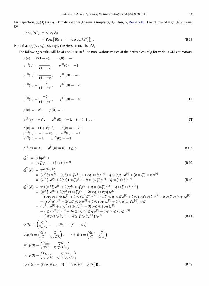
Note that θ (θ Aij)′ is simply the Hessian matrix of Aij.
The following results will be of use. It is useful to note various values of the derivatives of ρ for various GEL estimators.
ρ(v) = ln(1 − v), ρ(0) = −1
ρ[1](v) =−1
(1 − v), ρ[1](0) = −1
ρ[2](v) =−1
(1 − v)2, ρ[2](0) = −1
ρ[3](v) =−2
(1 − v)3, ρ[3](0) = −2
ρ[4](v) =−6
(1 − v)4, ρ[4](0) = −6 (EL)
ρ(v) = −ev, ρ(0) = 1
ρ[j](v) = −ev, ρ[j](0) = −1, j = 1, 2, . . . (ET)
ρ(v) = −(1 + v)2/2, ρ(0) = −1/2ρ[1](v) = −(1 + v), ρ[1](0) = −1ρ[2](v) = −1, ρ[2](0) = −1
ρ[j](v) = 0, ρ[j](0) = 0, j ≥ 3 (CUE)
q(1)i =
qρ[1]
= (q) ρ[1]+q ⊗ q′
ρ[2] (B.39)
q(2)i (β) =
2 qρ[1]=
2 qρ[1]
+ (q) ⊗ q′ρ[2]+ (q) ⊗ q′ρ[2]
+ q ⊗ (q′)ρ[2]+q ⊗ q′
⊗ q′ρ[3]
= (2 q)ρ[1]+ 2(q) ⊗ q′ρ[2]
+ q ⊗ (q′)ρ[2]+ q ⊗ q′
⊗ q′ρ[3] (B.40)
q(3)i (β) =
(2 q)ρ[1]
+ 2(q) ⊗ q′ρ[2]+ q ⊗ (q′)ρ[2]
+ q ⊗ q′⊗ q′ρ[3]
= (3 q)ρ[1]+ 2(2 q) ⊗ q′ρ[2]
+ 2(q) ⊗ (q′)ρ[2]
+ (q) ⊗ (q′)ρ[2]+ q ⊗ (2 q′)ρ[2]
+ (q) ⊗ q′⊗ q′ρ[3]
+ q ⊗ (q′) ⊗ q′ρ[3]+ q ⊗ q′
⊗ (q′)ρ[3]
+(2 q)ρ[2]
+ 2(q) ⊗ q′ρ[3]+ q ⊗ (q′)ρ[3]
+ q ⊗ q′⊗ q′ρ[4]
⊗ q′
= (3 q)ρ[1]+ 3(2 q) ⊗ q′ρ[2]
+ 3(q) ⊗ (q′)ρ[2]
+ q ⊗ (2 q′)ρ[2]+ 2q ⊗ (q′) ⊗ q′ρ[3]
+ q ⊗ q′⊗ (q)ρ[3]
+3(q) ⊗ q′ρ[3]
+ q ⊗ q′⊗ q′ρ[4]
⊗ q′ (B.41)
q(β0) =
g
0k×1
, q(β0)
′=g ′ 01×k
q(β) =
0l×l GG′
θ G′λ
, q(β0) =
0l×l GG′ 0k×k
2 q(β) =
0l×lm GG′
θ G′λ
3 q(β) =
0l×lmm G G′
θ G′λ
q′(β) =
(Vec[
0l×l G
])′ Vec[
G′
λ′G]. (B.42)
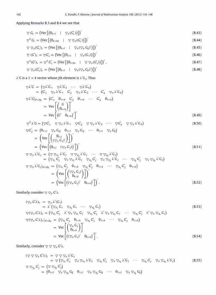
142 G. Kundhi, P. Rilstone / Journal of Multivariate Analysis 106 (2012) 118–146
Applying Remarks B.3 and B.4 we see that
Gi· =Vec
0k×l | θ (G
′
i·)′ (B.43)
2 Gi· =
Vec
0k×lm | θ (G
′
i·)′ (B.44)
θ (G′
i·)j· =Vec
0k×l | θ (θ Gij)
′′ (B.45)
(G′)i· = G′
·i =Vec
0l×l | θ (G·i)
′ (B.46)
2(G′)i· =
2 G′
·i =Vec
0l×lm | θ (G
′
·i)′
, (B.47)
θ (G′
·i)j· =Vec
0k×l | θ (θ Gji)
′′ (B.48)
λ′G is a 1 × k vector whose jth element is λ′G·j. Thus
λ′G =λ′G·1 λ′G·2 · · · λ′G·k
=G′
·1 θ λ′G·1 G′
·2 θ λ′G·2 · · · G′
·k θ λ′G·k
λ′G|β=β0 =G′
·1 01×k G′
·2 01×k · · · G′
·k 01×k
= Vec
G0k×k
′
= Vec
G′ 0k×k′′
(B.49)
2 λ′G =
G′
·1 θ λ′G·1 G′
·2 θ λ′G·2 · · · G′
·k θ λ′G·k
(B.50)
G′
·j =01×l θ G2j 01×l θ G1j · · · 01×l θ Glj
=
Vec
0l×l
(θ G·j)′
′
=
Vec
0l×l (θ G·j)
′′
(B.51)
θ λ′G·j = θ1
λ′G·j θ2λ′G·j · · · θk
λ′G·j
=θ1
G′
·j θ θ1λ′G·j θ2
G′
·j θ θ2λ′G·j · · · θk
G′
·j θ θkλ′G·j
θ λ′G·j|β=β0 =
θ1
G′
·j 01×k θ2G′
·j 01×k · · · θkG′
·j 01×k
=
Vec
(θ G·j)0k×k
′
=
Vec
(θ G·j)
′ 0k×k′′
. (B.52)
Similarly consider θ G′λ.
(θ G′λ)i· = θ λ′(G·i)
= λ′θ1
G·i θ2G·i · · · θk
G·i
(B.53)
(θ G′λ)j· =
θ1
G′
·j λ′θ θ1
G·j θ2G′
·j λ′θ θ2
G·j · · · θkG′
·j λ′θ θk
G·j
(θ G′λ)j·|β=β0 =
θ1
G′
·j 01×k θ2G′
·j 01×k · · · θkG′
·j 01×k
= Vec
θ G·j0k×k
′
= Vec
(θ G·j)′ 0k×k
′′
. (B.54)
Similarly, consider θ G′λ.
( θ G′λ)j· = θ λ′G·j
= θ1
G′
·j θ θ1λ′G·j θ2
G′
·j θ θ2λ′G·j · · · θk
G′
·j θ θkλ′G·j
(B.55)
θp G′
·j = θp G
′
·j
=01×l θ θp Glj 01×l θ θp G2j · · · 01×l θ θp Glj
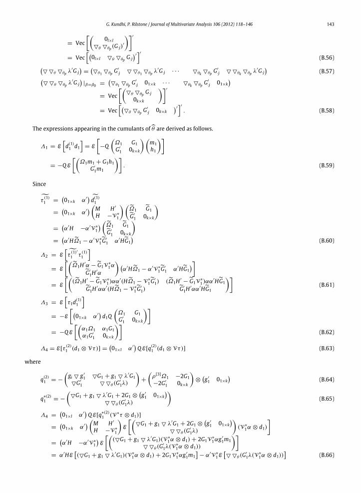
G. Kundhi, P. Rilstone / Journal of Multivariate Analysis 106 (2012) 118–146 143
= Vec
0l×lθ θp(G·j)
′
′
= Vec
0l×l θ θp G·j′′
(B.56) θ θp λ′G·j
=θ1
θp G′
·j θ1θp λ′G·j · · · θk
θp G′
·j θkθp λ′G·j
(B.57)
θ θp λ′G·j|β=β0 =
θ1
θp G′
·j 01×k · · · θkθp G
′
·j 01×k
= Vec
θ θp G·j
0k×k
′
= Vec
θ θp G′
·j 0k×k′′
. (B.58)
The expressions appearing in the cumulants ofθ are derived as follows.
Λ1 = Ed(1)1 d1
= E
−Q
Ω1 G1G′
1 0k×k
m1h1
= −QE
Ω1m1 + G1h1
G′
1m1
. (B.59)
Since
τ
(1)1 =
01×k α′
d(1)1
=01×k α′
M H ′
H −V∗
1
Ω1 G1G′
1 0k×k
=α′H −α′V∗
1
Ω1 G1G′
1 0k×k
=α′HΩ1 − α′V∗
1G′
1 α′HG1
(B.60)
Λ2 = Eτ
(1)′1 τ
(1)1
= E
Ω1H ′α −G1V∗
1αG′
1H′α
α′HΩ1 − α′V∗
1G′
1 α′HG1
= E
(Ω1H ′
−G1V∗
1 )αα′(HΩ1 − V∗
1G′
1) (Ω1H ′−G1V
∗
1 )αα′HG1G′
1H′αα′(HΩ1 − V∗
1G′
1)G′
1H′αα′HG1
(B.61)
Λ3 = Eτ1d
(1)1
= −E
01×k α′
d1Q
Ω1 G1G′
1 0k×k
= −QE
α1Ω1 α1G1α1G′
1 0k×k
(B.62)
Λ4 = E[τ(2)1 (d1 ⊗ Vτ)] =
01×l α′
QE[q(2)
1 (d1 ⊗ Vτ)] (B.63)
where
q(2)1 = −
gi g ′
1 G1 + g1 λ′G1G′
1 θ (G′
1λ)
+
ρ[3]Ω1 −2G1−2G′
1 0k×k
⊗g ′
1 01×k
(B.64)
q∗(2)1 = −
G1 + g1 λ′G1 + 2G1 ⊗
g ′
1 01×k
θ (G′
1λ)
(B.65)
Λ4 =01×l α′
QE[q∗(2)
1 (V∗τ ⊗ d1)]
=01×k α′
M H ′
H −V∗
1
E
G1 + g1 λ′G1 + 2G1 ⊗
g ′
1 01×k
θ (G′
1λ)
(V∗
1α ⊗ d1)
=α′H −α′V∗
1
E
(G1 + g1 λ′G1)(V
∗
1α ⊗ d1) + 2G1V∗
1αg′
1m1 θ (G
′
1λ(V∗
1α ⊗ d1))
= α′HE
(G1 + g1 λ′G1)(V
∗
1α ⊗ d1) + 2G1V∗
1αg′
1m1− α′V∗
1E θ (G
′
1λ(V∗
1α ⊗ d1))
(B.66)
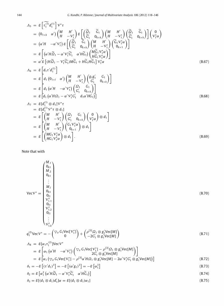
144 G. Kundhi, P. Rilstone / Journal of Multivariate Analysis 106 (2012) 118–146
Λ5 = Eτ
(1)1 d(1)
1
V∗τ
=01×k α′
M H ′
H −V∗
1
E
Ω1 G1G′
1 0k×k
M H ′
H −V∗
1
Ω1 G1G′
1 0k×k
0
V∗
1α
=α′H −α′V∗
1
E
Ω1 G1G′
1 0k×k
M H ′
H −V∗
1
G1V∗
1α0k×1
= E
α′HΩ1 − α′V∗
1G′
1 α′HG1 MG1V
∗
1α
HG1V∗
1α
= α′E
(HΩ1 − V∗
1G′
1)MG1 + HG1HG1V∗
1α (B.67)
Λ6 = Ed1τ ′d(1)
1
= E
d101×l α′
M H ′
H −V∗
1
g1g ′
1 G1G′
1 0k×k
= E
d1α′H −α′V∗
1
Ω1 G1G′
1 0k×k
= E
d1α′HΩ1 − α′V∗
1G′
1 d1α′HG1
(B.68)
Λ7 = E[d(1)1 ⊗ d1]V∗τ
= E[d(1)1 V∗τ ⊗ d1]
= E
M H ′
H −V∗
1
Ω1 G1G′
1 0k×k
0
V∗
1α
⊗ d1
= E
M H ′
H −V∗
1
G1V
∗
1α0k×1
⊗ d1
= E
MG1V
∗
1αHG1V
∗
1α
⊗ d1
. (B.69)
Note that with
VecV∗=
M.10k1M.20k1...
M.l0k10l1V∗
1.10l1V∗
1.20l1...
V∗
1.k
(B.70)
q(2)1 VecV∗
= −
θ G1Vec[V∗
1 ]
0
+
ρ[3]Ω1 ⊗ g ′
1Vec[M]
−2G′
1 ⊗ g ′
1Vec[M]
(B.71)
Λ8 = E[α1τ(2)1 ]VecV∗
= E
α1α′H −α′V∗
1
θ G1Vec[V∗
1 ] − ρ[3]Ω1 ⊗ g ′
1Vec[M]
2G′
1 ⊗ g ′
1Vec[M]
= E
α1θ G1Vec[V∗
1 ] − ρ[3]α′HΩ1 ⊗ g ′
1Vec[M] − 2α′V∗
1G′
1 ⊗ g ′
1Vec[M]
(B.72)
S1 = −E(τ ′d1)3
= −E
(α′g1)3
= −E
α31
(B.73)
S2 = Eα21
α′HΩ1 − α′V∗
1G′
1 α′HG1
(B.74)
S3 = E[(d1 ⊗ d1)d′
1]α = E[(d1 ⊗ d1)α1] (B.75)

G. Kundhi, P. Rilstone / Journal of Multivariate Analysis 106 (2012) 118–146 145
S4 = Eτ
(1)1 d1d′
1
τ
= −01×k α′
QE
Ω1 G1G′
1 0k×k
d1α1
= E
α′HΩ1 − α′V∗G′
1 α′HG1d1α1
= E
α′HΩ1m1α1 − α′V∗G′
1m1α1 + α′HG1h1α1
(B.76)
S5 = E[τ 21 d
′
1]
= E[α21d
′
1] (B.77)
E[q(2)1 ] = −
E[g1 g ′
1] E[G1 + g1 λ′G1]
E[G′
1] E[ θ (G′
1λ)]
+
ρ[3]E[Ω1 ⊗
g ′
1 01×k] −2E[G1 ⊗
g ′
1 01×k]
−2E[G′
1 ⊗g ′
1 01×k] 0k×km
(B.78)
τ(2)1 =
α′H −α′V∗
1
E[g1 g ′
1] E[G1 + g1 λ′G1]
E[G′
1] E[ θ (G′
1λ)]
+α′H −α′V∗
1
−ρ[3]E[Ω1 ⊗g ′
1 01×k] 2E[G1 ⊗
g ′
1 01×k]
2E[G′
1 ⊗g ′
1 01×k] 0k×km
(B.79)
q(3)= (3 q)ρ[1]
+ 3(2 q) ⊗ q′ρ[2]+ 3(q) ⊗ (q′)ρ[2]
+ q ⊗ (2 q′)ρ[2]+ 2q ⊗ (q′) ⊗ q′ρ[3]
+ q ⊗ q′⊗ (q)ρ[3]
+3(q) ⊗ q′ρ[3]
+ q ⊗ q′⊗ q′ρ[4]
⊗ q′
= −
0
2 G
2 G′
2θ G
′λ0
− 3
0 G
G′ θ G
′λ0
⊗ q′
− 30 GG′ 0
⊗ Vec
0 GG′ 0
′
− q ⊗ Vec
0 GG′
θ G′λ0
′′
+ 2qVec
0 GG′ 0
′
⊗ q′ρ[3]
+ qq′⊗ Vec
0 GG′ 0
′
ρ[3]+ 3
0 GG′ 0
⊗ q′
⊗ q′ρ[3]+ qq′
⊗ q′⊗ q′ρ[4]
= −
0
2 G
2 G′
2θ G
′λ0
− 3
0 G
G′ θ G
′λ0
⊗ q′
− 30 GG′ 0
⊗ Vec
0 GG′ 0
′
− qVec
0 GG′
θ G′λ0
′′
+ 2qVec
0 GG′ 0
′
⊗ q′ρ[3]
+ qq′⊗ Vec
0 GG′ 0
′
ρ[3]+ 3
0 GG′ 0
⊗ q′
⊗ q′ρ[3]+ qq′
⊗ q′⊗ q′ρ[4]. (B.80)
Note that the rows of q(j) are the vectorization of the jth order derivatives of q. By Young’s Theorem we have that, form× 1matrices, a, b and c we have, q(3)(a ⊗ b ⊗ c) = q(3)(b ⊗ a ⊗ c) = q(3)(b ⊗ c ⊗ a). Since
Vτ ⊗−→V =
0lm2×1
V∗
1α ⊗−→V
(B.81)
q(3)Vτ ⊗−→V = q∗(3)V∗
1α ⊗−→V
∗
(B.82)
where
q∗(3)= −
2 G
2θ G
′λ0
− 3
G
θ G′λ0
⊗ q′
− 30 GG′ 0
⊗ Vec
G0
′
− qVec
G θ G
′λ0
′′
+ 2qVec
G0
′
⊗ q′ρ[3]+ qq′
⊗ Vec
G0
′
ρ[3]+ 3
G0
⊗ q′
⊗ q′ρ[3]. (B.83)
By inspection of the zeros in q∗(3) and−→V1
∗
we see that
q∗(3)V∗
1α ⊗−→V1
∗
= −
2θ GV∗
1α ⊗−→V1
∗
10
− 0 − 3
0
G′⊗ Vec [G]′ V∗
1α ⊗−→M
− 0 + 2qVec [G]′ ⊗ g ′ρ[3]α ⊗
−→M
+ qg ′⊗ Vec [G]′ ρ[3]V∗
1α ⊗−→M + 3
G0
⊗ g ′
⊗ g ′ρ[3]V∗
1α ⊗−→M . (B.84)
146 G. Kundhi, P. Rilstone / Journal of Multivariate Analysis 106 (2012) 118–146
Thus
Λ9 = τ(3)1
V∗τ ⊗
−→V1
∗
=−α′H α′V∗
Eq∗(3)V∗
1α ⊗−→V1
= α′HE[2θ G](V∗
1α ⊗−→V∗
1 ) − 3α′V∗
1E[G′⊗ Vec [G]′](V∗
1α ⊗−→M ) − 2α′HE[gVec [G]′ ⊗ g ′
]
× (V∗
1α ⊗−→M )ρ[3]
− α′HE[gg ′⊗ Vec [G]′](V∗
1α ⊗−→M )ρ[3]
− 3α′HE[G ⊗ g ′⊗ g ′
](V∗
1α ⊗−→M )ρ[3]
= α′HE[2θ G](V∗
1α ⊗−→V∗
1 ) − 3α′V∗
1E[G′⊗ Vec [G]′](V∗
1α ⊗−→M )
− α′H2E[gVec [G]′ ⊗ g ′
] + E[gg ′⊗ Vec [G]′] + 3E[G ⊗ g ′
⊗ g ′](V∗
1α ⊗−→M )ρ[3]. (B.85)
References
[1] T. Amemiya, The n−2-order mean squared errors of the maximum likelihood and the minimum logit chi-square estimator, Annals of MathematicalStatistics 8 (1980) 488–505.
[2] O.E. Barndorff-Nielson, D.R. Cox, Asymptotic Techniques for Use in Statistics, Chapman and Hall, New York, NY, 1989.[3] R.N. Bhattacharya, J.K. Ghosh, On the validity of the formal Edgeworth expansion, The Annals of Statistics 6 (2) (1978) 434–451.[4] R.N. Bhattacharya, R.R. Rao, Normal Approximation and Asymptotic Expansion, Wiley, New York, 1976.[5] F. Bravo, Empirical likelihood based inference with applications to some econometric models, Econometric Theory 20 (2004) 231–264.[6] J.M. Chambers, On methods of asymptotic approximation for multivariate distributions, Biometrika 50 (3–4) (1967) 367–383.[7] R. Davidson, J.G. MacKinnon, Bootstrap tests: how many bootstraps? Econometric Reviews 19 (2000) 55–68.[8] J.K. Ghosh, B.K. Sinha, H.S.Wieand, Second-order efficiency of theMLEwith respect to any bowl-shaped loss function, Annals ofMathematical Statistics
8 (1980) 506–521.[9] Peter Hall, The Bootstrap and the Edgeworth Expansion, Springer-Verlag, New York, NY, 1992.
[10] P. Hall, J.L. Horowitz, Bootstrap critical values for tests based on generalized-method-of-moments estimators, Econometrica 64 (4) (1996) 891–916.[11] L.P. Hansen, Large sample properties of generalized method of moments estimators, Econometrica 50 (1982) 1029–1054.[12] B.E. Hansen, in: D. Corbae, S.N. Durlauf, B.E. Hansen (Eds.), Edgeworth Expansions for the Wald and GMM Statistics for Nonlinear Restrictions,
Econometric Theory and Practice, 2006.[13] L.P. Hansen, J. Heaton, A. Yaron, Finite sample properties of some alternative GMM estimators, Journal of Business and Economic Statistics 14 (1996)
262–280.[14] G. Imbens, One-step estimators for over-identified generalized method of moments models, The Review of Economic Studies 64 (3) (1997) 359–383.[15] G. Kundhi, P. Rilstone, The third order bias of nonlinear estimators, Communications in Statistics; Theory and Methods 37 (16) (2008) 2617–2633.[16] O. Linton, Edgeworth approximations for semiparametric instrumental variable estimators and test statistics, Manuscript, London School of
Economics, 2000.[17] P. McCullagh, Tensor Methods in Statistics, Chapman and Hall, New York, NY, 1987.[18] W. Newey, D. McFadden, Large Sample Estimation and Hypothesis Testing, in: Handbook of Econometrics, vol. 4, North Holland, Amsterdam, 1994,
pp. 2111–2245.[19] Whitney K. Newey, Richard Smith, Higher order properties of GMM and generalized empirical likelihood estimators, Econometrica 72 (1) (2004)
219–255.[20] J. Pfanzagl, W. Wefelmeyer, A third-order optimum property of the maximium likelihood estimator, Journal of Multivariate Analysis 10 (1978) 1–29.[21] P.C.B. Phillips, A general theorem in the theory of asymptotic expansions as approximations to the finite sample distributions of econometric
estimators, Econometrica 45 (6) (1977) 1517–1534.[22] P.C.B. Phillips, J.Y. Park, On the formulation of Wald tests of nonlinear restrictions, Econometrica 56 (5) (1988) 1065–1083.[23] J. Qin, J. Lawless, Empirical likelihood and general estimating equations, Annals of Statistics 22 (1) (1994) 300–325.[24] Paul Rilstone, V.K. Srivastava, Aman Ullah, The second-order bias and mean squared error of nonlinear estimators, Journal of Econometrics 75 (2)
(1996) 369–395.[25] Paul Rilstone, Aman Ullah, Corrigendum to: the second–order bias and mean squared error of non-linear estimators, Journal of Econometrics 124 (1)
(2005) 203–204.[26] Thomas J. Rothenberg, Approximating the distributions of econometric estimators and test statistics, in: Z. Griliches, M.D. Intriligator (Eds.),
in: Handbook of Econometrics, vol.2, Elsevier Science Inc., New York, NY, 1984, ch. 15.[27] J.D. Sargan, Econometric estimators and the Edgeworth approximation, Econometrica 44 (3) (1976) 421–448.[28] D.L. Wallace, Asymptotic approximations to distributions, Annals of Mathematical Statistics 29 (1958) 635–654.


