Embed Size (px)
Citation preview
PSYCHOMETRIC IMPLICATIONS OF CORRECTIONS FOR
ATTENUATION AND RESTRICTION OF RANGE FOR SELECTION
VALIDATION RESEARCH
CARL CHRISTIAAN THERON
DISSERTATION PRESENTED FOR THE DEGREE
OF
DOCTOR OF PHILOSOPHY
AT THE
UNIVERSITY OF STELLENBOSCH
PROMOTER: PROF JCD AUGUSTYN
MARCH1999

DECLARATION
I, the undersigned, hereby declare that the work contained in this dissertation is my
own original work and that I have not previously in its entirety or in part submitted it
at any university for a degree
Date: 05-02-99
ii Stellenbosch University http://scholar.sun.ac.za

OPSOMMING I I
iii
Die toestande waaronder keuringsprosedures tipes gevalideer word en die toestande waaronder die
prosedure uiteindelik gebruik word, verskil normaalweg tot so 'n mate dat die relevansie van die
bevindinge in die gedrang kom. Statistiese korreksies vir die geldigheidskoeffisient is algemeen
beskikbaar. Die res van die argument in terme waarvan 'n keuringsprosedure ontwikkel en regverdig
word kan egter ook verwring word deur dieselfde verskille tussen die toestande waaronder die
keuringsprosedure gesimuleer word en die waaronder die prosedure uiteindelik gebruik word. Relatief
min kommer bestaan skynbaar egter ten opsigte van die oordraagbaarheid van die besluitnemingsfunksie
wat onder die gesimuleerde toestande ontwikkel is of ten opsigte van die verkree beskrywings van nut en
billikheid. Hierdie toedrag van sake val ietwat vreemd op. Die eksteme geldigheidprobleme geassosieer
met validasie-ontwerpe is redelik goed gedokumenteer. Dit is dus nie asof die psigometrika-literatuur
onbewus is van die probleem wat by die veralgemening van resultate van geldigheidstudies ter sprake is
nie. Die besluitnemingsfunksie is waarskynlik die spil waarom die keuringsprosedure draai daarin dat dit
die onderliggende prestasie-teorie vergestalt, maar meer belangrik, daarin dat dit die daadwerklike
aanvaarding en verwerping van applikante bepaal. Indien statistiese korreksies tot die
geldigheidskoeffisient beperk word bly die besluitnemingsfunksie onveranderd, alhoewel dit ook
moontlik verwring mag word deur dieselfde faktore wat sydigheid in die geldigheidskoeffisient te weeg
bring. Dieselfde logika geld ook ten opsigte van die evaluasie van die besluitnemingsfunksie in terme
van nut en billikheid. Indien slegs die geldigheidskoeffisient gekorrigeer word bly d.e "bottom-line"
evaluasie van die keuringsprosedure onveranderd. Prakties gesproke dus, verander niks indien statistiese
korreksies tot die geldigheidskoeffisient beperk word. Die fundamentele navorsingsdoelstelling is om
vas te stel of verskille tussen die toestande waaronder die keuringsprosedure gevalideer word, en die
toestande waaronder die prosedure uiteindelik gebruik word, sydigheid te weeg bring in die maatstawwe
wat vereis word om die keuringsprosedure te spesifiseer en te regverdig; om toepaslike statistiese
korreksies vir die geldigheidskoeffisient, besluitnnemingsreel en beskrywings van nut en billikheid af te
lei ten einde die kontekste van simulasie/ validasie en toepassing te versoen; en om vas te stel of sodanige
korreksies wel in validasie-navorsing toegepas behoort te word. Die studie verskaf geen
ongekwalifiseerde antwoord op die vraag of korreksies vir die verskeie vorms van variansie-inperking
en/ of kriterium onbetroubaarheid op die geldigheidskoeffisient, die standaardfout van die
geldigheidskoefisient of die parameters van die regressie van die kriterium op die voorspeller toegepas
behoort te word nie. Die korreksies affekteer wel besluite aangaande die geldigheid van prestasie
hipoteses onder spesifieke toestande. Die korreksies het ook onder bepaalde toestande 'n effek op
besluite aangaande applikante deur hul effek op die regressiekoeffisiente en/ of die
standaardskattingsfout.
Stellenbosch University http://scholar.sun.ac.za
IV
ABSTRACT
The conditions under which selection procedures are typically validated and those prevailing at the
eventual use of a selection procedure normally differ to a sufficient extent to challenge the relevance of
the validation research evidence. Statistical corrections to the validity coefficient are generally available.
The remainder of the argument in terms of which a selection procedure is developed and justified could,
however, also be biased by any discrepancy between the conditions under which the selection procedure
is simulated and those prevailing at the eventual use of the selection procedure. Relatively little concern,
however, seem to exist for the transportability of the decision function derived from the selection
simulation or the descriptions/ assessments of selection decision utility and fairness. This seems to be a
somewhat strange state of affairs. The external validity problems with validation designs are reasonably
well documented. It is thus not as if the psychometric literature is unaware of the problem of
generalizing validation study research fmdings to the eventual area of application. The decision function
is probably the pivot of the selection procedure in that it firstly captures the underlying performance
theory, but more importantly from a practical perspective, because it guides the actual accept and reject
choices of applicants. Restricting the statistical corrections to the validity coefficient would leave the
decision function unaltered even though it might also be distorted by the same factors affecting the
validity coefficient. Basically the same logic also applies to the evaluation of the decision rule in terms of
selection utility and fairness. Correcting only the validity coefficient would leave the "bottom-line"
evaluation of the selection procedure unaltered. Restricting the statistical corrections to the validity
coefficient basically means that practically speaking nothing really changes. The fundamental research
objective is to determine whether any discrepancy between the conditions under which the selection
procedure is simulated and those prevailing at the eventual use of the selection procedure produces bias
in estimates required to specify and justify the procedure; to delineate appropriate statistical corrections
of the validity coefficient, decision rule and descriptions/ assessments of selection decision utility and -1< fairness, required to align the contexts of evaluation/validation and application; and to determine
whether the corrections should be applied in validation research. The study provides no unqualified
answers to the question whether corrections for various forms of range restriction and/ or criterion
unreliability should be applied to the validity coefficient, the standard error of the validity coefficient or
the parameters of the regression of the criterion on the predictor. Under specific conditions the
corrections do affect decisions on the validity of performance hypotheses due to its effect on decisions
on the significance of the uncorrected versus the corrected validity coefficient. Under specific conditions
the corrections do affect decisions on applicants, especially when selection decisions are not restricted by
selection quotas, due to its effect on the slope and intercept parameters of the regression of Y on X,
and/ or due to its effect on the standard error of estimate.
Stellenbosch University http://scholar.sun.ac.za

v
ACKNOWLEDGEMENTS
It takes more than one person to complete a doctoral thesis and nowhere is it more true than in my case.
I consequently would like to thank the following people and institutions who have made valuable and
much appreciated contributions to the completion of this research.
\f'
My supervisor, Prof JCD Augustyn, for his support, guidance and encouragement and for teaching me
what true loyalty to colleagues, friends and family really means.
\{1
My wife, Antionette and my daughters Michelle and Anelle, for their love, support and encouragement.
\f'
Prof J Schepers for his invaluable advice, encouragement and recommendations.
\f'
Prof JM du T oit who inculcated my love and appreciation for psychometrics.
\f'
My parents for their love, support and investment in me.
My colleagues, Coen, Johan, Gawie & Henry who were prepared to take over my lecturing
responsibilities so as to enable me to take the sabbatical to complete this research.
\f'
Gawie Cillie for his willingness to sacrifice long hours in strategic consultation and for his valuable
advice and support.
\f'
Colleagues from the Department of Statistics for their concern, support and advice.
\f'
The internal and external examiners for pointing out deficiencies in the original manuscript and for their
recommendations and advice.
The financial assistance of the Centre for Science Development towards this research is hereby
acknowledged. Opinions expressed in this thesis and conclusions arrived at, are those of the author and
are not necessarily to be attributed to the Centre for Science Development.
Stellenbosch University http://scholar.sun.ac.za
vi
TABLE OF CONTENTS
PAGE
DECLARATION .. 11
... OPSOMMING ill
ABS1RACT lV
ACKNOWLEDGEMENTS v
TABLE OF CONTENTS Vl
... LIST OF FIGURES XVill
LIST OFT ABLES ..
XXXl1
1. INTRODUCTION, RESEARCH OBJECTIVE AND OVERVIEW OF THE
STUDY
1.1 Introduction 2
1.2 Personnel Selection 6
1.2.1 An Operational Perspective On Personnel Selection 8
1.2.2 A Strategic Perspective On Personnel Selection 19
1.2.3 An Equity Perspective On Personnel Selection 25
1.3. Summary And Research Objectives 28
1.4. Structural Outline Of Dissertation 31
2. MEASUREMENT THEORY
2.1 Constructs 35
2.2 The Nature Of Measurement 37
2.3. Measurement Theory 41
2.4 Notation 42
2.5 Classical Measurement Theory 43
2.5.1 Reliability 47
Stellenbosch University http://scholar.sun.ac.za
VII
2.5.1.1 Reliability Estimates 50
2.5.1.1.1 Test-Retest Method 54
2.5.1.1.2 Internal Analysis Method 55
2.5.1.1.3 Parallel Forms Method 94
2.5.2 validity 95
2.6 Summary 104
3. SEPARATE AND COMBINED CORRECTIONS TO THE VALIDITY
COEFFICIENT FOR THE ATTENUATING EFFECT OF THE
UNRELIABILITY OF MEASUREMENTS AND RESTRICTION OF RANGE
3.1. The Need For Corrections To The Validity Coefficient For The
Attenuating Effect Of The Unreliability Of Measurements And
Restriction Of Range
3.2 The Validity Coefficient Corrected For The Attenuating Effect Of The
Unreliability Of The Criterion Measurements
3.3 The Validity Coefficient Corrected For The Attenuating Effect Of
Explicit Or Implicit Restriction Of Range
3.3.1 Univariate Selection
3.3.1.1
3.3.1.2
3.3.1.3
The Effect Of Case 1 [Case B] Restriction Of Range
On The Validity Coefficient
The Effect Of Case 2 [Case A] Restriction Of Range
On The Validity Coefficient
The Effect Of Case 3 [Case C] Restriction Of Range
On The Validity Coefficient
3.3.2 Multivariate Selection
3.3.3 Accuracy Of Corrections To The Validity Coefficient For The
Attenuating Effect Of Explicit Or Implicit Restriction Of Range
3.4 The Validity Coefficient Corrected For The Joint Attenuating Effect Of
Explicit Or Implicit Range Restriction And The Unreliability Of The
Criterion Measurements
3.5 Summary
106
113
117
117
120
123
125
138
138
143
156
Stellenbosch University http://scholar.sun.ac.za

VIII
4. STATISTICAL INFERENCE REGARDING CORRELATIONS CORRECTED
FOR THE SEPARATE AND COMBINED ATTENUATING EFFECT OF
RESTRICTION OF RANGE AND CRITERION UNRELIABILITY
4.1 Inferential Statistics In Validation Research
4.2. The Need For Information On The Sampling Distribution Of The
Validity Coefficient Corrected For The Attenuating Effect Of The
Unreliability Of Measurements And/ or Restriction Of Range
4.3 Different Procedures For Investigating The Sampling Distributions Of
Statistical Estimators
4.4 Non-Distribution Free Estimates Of Statistical Error
4.4.1 Delta Method
4.5 Distribution Free Estimates Of Statistical Error
4.5.1 Bootstrap Estimates Of Statistical Error
4.5.1.1 Bootstrap Confidence Intervals
4.5.1.2 Bootstrap Hypothesis Testing
4.5.1.3 Bootstrap Sample Size Requirements
4.5.2 Jackknife Estimates Of Statistical Error
4.6 Expressions For The Standard Error Of The Pearson Correlation
Coefficient
4.6.1 Obtained, Uncorrected First-Order Pearson Correlation Coefficient
4.6.2 Pearson Correlation Coefficient Corrected For Criterion And
Predictor Unreliability
4.6.3 Pearson Correlation Coefficient Corrected For Criterion
Unreliability Only
4.6.4 Pearson Correlation Coefficient Corrected For Case 1 [Case B]
Restriction Of Range
4.6.5 Pearson Correlation Coefficient Corrected For Case 2 [Case A]
Restriction Of Range
4.6.6 Pearson Correlation Coefficient Corrected For Case C Restriction
Of Range
4.6.7 Pearson Correlation Coefficient Double Corrected For Restriction
Of Range And Criterion Unreliability
4.7 Summary
157
159
160
160
161
162
162
163
166
167
167
168
168
170
173
186
186
192
201
214
Stellenbosch University http://scholar.sun.ac.za
IX
5. EFFECT OF STATISTICAL CORRECTIONS OF THE VALIDITY
COEFFICIENT ON DECISIONS ON THE NULL HYPOTHESES
5.1 The Logic Of [Fisherian] Statistical Significance Testing
5.2 Effect Of Corrections For Attenuation And/or Range Restrication To
The Pearson Correlation Coefficient On Decisions On Statistical Null
Hypotheses
5.3 Effect Of Corrections For Attenuation And/ or Range Restriction To The
Pearson Correlation Coefficient On The Empirically Derived Exceedence
Probabilities ab [Or Achieved Significance Level, ASL]
5.3.1 Effect Of Corrections For Attenuation To The Pearson Correlation
Coefficient On The Empirically Derived Exceedence Probabilities
Ub
5.3.1.1
5.3.1.2
5.3.1.3
The Reliability Coefficient Given A Priori By
Theoretical Assumption Or Previously Accepted
Knowledge
The Reliability Coefficient Obtained From An
Independent Data Set
The Reliability Coefficient Obtained From The Same
Data Set As p A [X,Y]
5.3.2 Effect Of Corrections For Restriction Of Range To The Pearson
Correlation Coefficient On The Empirically Derived Exceedence
Probabilities ab
5.3.2.1 Case 2 [Case A] Restriction Of Range
3.3.2.2 Case 3 [Case C] Restriction Of Range
5.3.3 Effect Of Corrections For Criterion Unreliability And Range
Restriction To The Pearson Correlation Coefficient On The
Empirically Derived Exceedence Probabilities ab
5.4 Effect Of Corrections For Attenuation And/ or Range Restriction To The
Pearson Correlation Coefficient On The A Priori Probabilities [1-PJ Or
Power Of The Tests Of Ho
215
217
224
224
224
226
230
234
234
237
241
246
Stellenbosch University http://scholar.sun.ac.za
5.4.1 Effect Of Corrections For Attenuation To The Pearson Correlation
Coefficient On The A Priori Probabilities [1-PJ Or Power Of The
Tests OfHo
5.4.1.1
5.4.1.2
5.4.1.3
The Reliability Coefficient Given A Priori By
Theoretical Assumption Or Previously Accepted
Knowledge
The Reliability Coefficient Obtained From An
Independent Sample
The Reliability Obtained From The Same Sample As
p~[X,Y]
5.4.2 Effect Of Corrections For Restriction Of Range To The Pearson
Correlation Coefficient On The A Priori Probabilities [1-PJ Or
Power Of The Tests Of Ho
5.4.2.1
5.4.2.2
Case 2 [Case A] Restriction Of Range
Case C Restriction Of Range
5.4.3 Effect Of Double Corrections For Attenuation And Restriction Of
Range To The Pearson Correlation Coefficient On The A Priori
Probabilities [1-PJ Or Power Of The Tests Of Ho
5.5 Summary
X
247
247
248
249
250
250
252
256
256
6. EFFECT OF STATISTICAL CORRECTIONS TO THE VALIDITY
COEFFICIENT ON THE PARAMETERS OF THE DECISION FUNCTION
6.1 The Decision Function In Personnel Selection
6.2 Effect Of Statistical Corrections For Range Restriction And/ or Random
Measurement Error In The Criterion On The Decision Function
6.2.1 Effect Of Statistical Corrections For Random Measurement Error
On The Decision Function
6.2.1.1 Effect Of Statistical Corrections For Random
Measurement Error In The Criterion On The Decision
Function
259
267
268
268
Stellenbosch University http://scholar.sun.ac.za
6.2.1.2 Effect Of Statistical Corrections For Random
Measurement Error In Both The Criterion And The
Predictor On The Decision Function
6.2.2 Effect Of Statistical Corrections For Restriction Of Range On The
Decision Function
6.2.2.1
6.2.2.2
6.2.2.3
Case 1 [Case B] Restriction Of Range
Case 2 [Case A] Restriction Of Range
Case 3 [Case C] Restriction Of Range
6.2.3 Effect Of The Joint Correction For Case 2 [Case A] Restriction Of
Range And Criterion Unreliability On The Decision Function
6.3 Concluding Comments
6.4 Summary
xi
275
286
286
293
293
310
315
315
7. CONCLUSIONS AND RECOMMENDATIONS FOR FURTHER RESEARCH
7.1 Conclusions
7.1.1 Reviewing The Necessity And Significance Of The Research
7.1.2 Research Objectives
7.1.3 Methodology
7.1.4 Summary Of Results
7.1.4.1 The Effect Of Separate And Combined Statistical
Corrections For Restriction Of Range And Random
Measurement Error On The Magnitude Of The
Validity Coefficient
7.1.4.1.1 The Effect Of The Correction For
Criterion Unreliability Only On The
Magnitude Of The Validity Coefficient
7.1.4.1.2 The Effect Of The Correction Case 1 [Case
B] Restriction Of Range On The
Magnitude Of The Validity Coefficient
7.1.4.1.3 The Effect Of The Correction For Case 2
[Case A] Restriction Of Range On The
Magnitude Of The Validity Coefficient
316
316
320
321
322
322
322
322
323
Stellenbosch University http://scholar.sun.ac.za

7.1.4.2
7.1.4.3
7.1.4.1.4 The Effect Of The Correction For Case C
Restriction Of Range On The Magnitude
Of The Validity Coefficient
7.1.4.1.5 The Effect Of The Joint Correction For
Case 2 [Case A] Restriction Of Range On
X And Criterion Unreliability On The
Magnitude Of The Validity Coefficient
The Effect Of Separate And Combined Statistical
Corrections For Restriction Of Range And Random
Measurement Error On The Magnitude Of The
Standard Error Of The Pearson Correlation Coefficient
7.1.4.2.1 The Effect Of The Correction For
Criterion Unreliability Only On The
Magnitude Of The Standard Error Of The
Pearson Correlation Coefficient
7.1.4.2.2 The Effect Of The Correction For Case 1
[Case B] Restriction Of Range On The
Magnitude Of The Standard Error Of The
Pearson Correlation Coefficient
7.1.4.2.3 The Effect Of The Correction For Case 2
[Case A] Restriction Of Range On The
Magnitude Of The Standard Error Of The
Pearson Correlation Coefficient
7.1.4.2.4 The Effect Of The Correction For Case 3
[CaseC] Restriction Of Range On The
Magnitude Of The Standard Error Of The
Pearson Correlation Coefficient
7.1.4.2.5 The Effect Of The Joint Correction For
Case 2 [Case A] Restriction Of Range On
X And Criterion Unreliability On The
Magnitude Of The Standard Error Of The
Pearson Correlation Coefficient
The Effect Of Separate And Combined Statistical
Corrections For Restriction Of Range And Random
Measurement Error On The Magnitude Of The
Empirically Derived Exceedence Probability ab
xii
323
324
325
325
327
327
328
329
331
Stellenbosch University http://scholar.sun.ac.za
7.1.4.4
7.1.4.3.1 The Effect Of The Correction For
Criterion Unreliability Only On The
Magnitude Of The Empirically Derived
Exceedence Probability
7.1.4.3.1.1 The Reliability Coefficient
Given A Priori By Theoretical
Assumption Or Previously
Accepted Knowledge
7.1.4.3.1.2 The Reliability Coefficient
Obtained From An
Independent Data Set
7.1.4.3.1.3 The Reliability Coefficient
Obtained From The Same
Data Set
7.1.4.3.2 The Effect Of The Correction For Case 1
[Case B] Restriction Of Range On The
Magnitude Of The Empirically Derived
Exceedence Probability
7.1.4.3.3 The Effect Of The Correction For Case 2
[Case A] Restriction Of Range On The
Magnitude Of The Empirically Derived
Exceedence Probability
7.1.4.3.4 The Effect Of The Correction For Case
3[i] [Case C[i]] Restriction Of Range On
The Magnitude Of The Empirically
Derived Exceedence Probability
7.1.4.3.5 The Effect Of The Joint Correction For
Case 2 [Case A] Restriction Of Range On
X And Criterion Unreliability On The
Magnitude Of The Empirically Derived
Exceedence Probability
The Effect Of Separate And Combined Statistical
Corrections For Restrictions Of Range And Random
Measurement Error On The Magnitude Of The A
Priori Probability Of Rejecting HO If HO Is False
xiii
331
331
331
332
332
332
333
334
335
Stellenbosch University http://scholar.sun.ac.za
7.1.4.5
7.1.4.4.1 The Effect Of The Correction For
Criterion Unreliability Only On The
Magnitude Of The A Priori Probability Of
Rejecting HO If HO Is False
7.1.4.4.1.1 The Reliability Coefficient
Given A Priori By Theoretical
Assumption Or Previously
Accepted Knowledge
7.1.4.4.1.2 The Reliability· Coefficient
Obtained From An
Independent Sample
7.1.4.4.1.3 The Reliability Coefficient
Obtained From The Same
Sample
7.1.4.4.2 The Effect Of The Correction For Case 1
[Case B] Restriction Of Range On The
Magnitude Of The A Priori Probability Of
Rejecting HO If HO Is False
7.1.4.4.3 The Effect Of The Correction For Case 2
[Case A] Restriction Of Range On The
Magnitude Of The A Priori Probability Of
Rejecting HO If HO Is False
7.1.4.4.4 The Effect Of The Correction For Case
3[i] [Case C[i]] Restriction Of Range On
The A Priori Probability Of Rejecting HO If
HO Is False
7.1.4.4.5 The Effect Of The Joint Correction For
Case 2 [Case A] Restriction Of Range On
X And Criterion Unreliability On The
Magnitude Of The A Priori Probability Of
Rejecting HO If HO Is False
The Effect Of Separate And Combined Statistical
Corrections For Restriction Of Range And Random
Measurement Error On The Magnitude Of The
Intercept And Slope Parameters Of The Regression Of
The Criterion On The Predictor
XIV
335
335
335
335
336
336
336
337
337
Stellenbosch University http://scholar.sun.ac.za
7.1.4.6
7.1.4.5.1 The Effect Of The Correction For
Criterion Unreliability Only On The
Magnitude Of The Intercept And Slope
Parameters Of The Regression Of The
Criterion On The Predictor
7.1.4.5.2 The Effect Of Case 1 [Case B] Restriction
Of Range On The Magnitude Of The
Intercept And Slope Parameters Of The
Regression Of The Criterion On The
Predictor
7.1.4.5.3 The Effect Of The Correction For Case 2
[Case A] Restriction Of Range On The
Magnitude Of The Intercept And Slope
Parameters Of The Regression Of The
Criterion On The Predictor
7.1.4.5.4 The Effect Of The Correction For Case
3[i] [Case C[i]] Restriction Of Range On
The Magnitude Of The Intercept And
Slope Parameters Of The Regression Of
The Criterion On The Predictor
7.1.4.5.5 The Effect Of The Joint Correction For
Case 2 [Case A] Restriction Of Range On
X And Criterion Unreliability On The
Magnitude Of The Intercept And Slope
Parameters Of The Regression Of The
Criterion On The Predictor
The Effect Of Separate And Combined Statistical
Corrections For Restriction Of Range And Random
Measurement Error On The Magnitude Of The
Standard Error Of Estimate Of The Regression Of The
Criterion On The Predictor
7.1.4.6.1 The Effect Of The Correction For
Criterion Unreliability Only On The
Magnitude Of The Standard Error Of
Estimate Of The Regression Of The
Criterion On The Predictor
XV
337
338
339
340
341
342
342
Stellenbosch University http://scholar.sun.ac.za
7.1.4.6.2 The Effect Of The Correction For Case 1
[Case B] Restriction Of Range On The
Magnitude Of The Standard Error Of
Estimate Of The Regression Of The
Criterion On The Predictor
7.1.4.6.3 The Effect Of The Correction For Case 2
[Case A] Restriction Of Range On The
Magnitude Of The Standard Error Of
Estimate Of The Regression Of The
Criterion On The Predictor
7.1.4.6.4 The Effect Of The Correction For Case
3[i] [Case C[i]] Restriction Of Range On
The Magnitude Of The Standard Error Of
Estimate Of The Regression Of The
Criterion On The Predictor
7.1.4.6.5 The Effect Of The Joint Correction For
Case Restriction Of Range On X And
Criterion Unreliability On The Magnitude
Of The Magnitude Of The Standard Error
Of Estimate Of The Regression Of The
Criterion 0 The Predictor
7.1.5 Synopsis Of Findings
7.2 Recommendations For Further Research
7.2.1 The Effect Of Statistical Corrections For Restriction Of Range
And/ or Criterion Unreliability On Utility Assessments
7 .2.1.1 Payoff Defined In Terms Of The Validity Coefficient
7 .2.1.2 Payoff Defined In Terms Of The Success Ratio
7.2.1.3 Payoff Defined In Terms Of The Expected
Standardized Criterion Score
7.2.1.4
7.2.1.5
7.2.1.6
Payoff Defined In Terms Of A Monetary Valued
Criterion
Refining Payoff Defined In Terms Of A Monetary
Valued Criterion
Analysis Of Selection Utility In Terms Of Risk
xvi
343
344
345
346
347
348
348
350
351
353
355
359
367
Stellenbosch University http://scholar.sun.ac.za
7.2.2 The Effect Of Corrections For Random Measurement Error And
Nonrandom Selection On Fairness Assessments Of Selection
Procedures
7 .2.2.1 The Cleary Model Of Selection Fairness
7.2.2.2 The Einhorn-Bass Model Of Selection Fairness
7.2.2.3 The Thorndike Model Of Selection Fairness
7.2.3 Additional Specific Recommendations For Further Research
REFERENCES
APPENDIX A
xvii
369
370
371
372
372
374
385
Stellenbosch University http://scholar.sun.ac.za
Figure 2.1
Figure 3.1
Figure 3.2
Figure 3.3
Figure 3.4
Figure 3.5
Figure 3.6
Figure 3.7
Figure 3.8
Figure 3.9
Figure 3.10
LIST OF FIGURES
The five pivotal linkages in the interpretive argument
underlying selection instrument score interpretation in the
context of personnel selection
The partially disattenuated validity coefficient as a function of
p[X,Y] and Ptt y
The partially disattenuated validity coefficient as a function of
p[X,Y] and Ptt y
The validity coefficient corrected for Case 1 [Case B]
restriction of range as a function of K and p[x,y]
The validity coefficient corrected for Case 1 [Case B]
restriction of range as a function of K and p[ x,y]
The validity coefficient corrected for Case 2 [Case A]
restriction of range as a function of K and p[ x,y]
The validity coefficient corrected for Case 2 [Case A]
restriction of range as a function of K and p[ x,y]
The validity coefficient corrected for Case 3[i] [Case C[i]]
restriction of range as a function of K, p[y,z] and p[x,y] for
p[x,z] fixed at 0.2
The validity coefficient corrected for Case 3[i] [Case C[i]]
restriction of range as a function of K, p[y,z] and p[x,y] for
p[x,z] fixed at 0.2
The validity coefficient corrected for Case 3[i] [Case C[i]]
restriction of range as a function of K, p[y,z] and p[x,y] for
p[x,z] fixed at 0.5
The validity coefficient corrected for Case 3[i] [Case C[i]]
restriction of range as a function of K, p[y,z] and p[ x,y] for
p[x,z] fixed at 0.5
XV Ill
PAGE
101
118
118
122
122
126
126
131
131
132
132
Stellenbosch University http://scholar.sun.ac.za
Figure 3.11
Figure 3.12
Figure 3.13
Figure 3.14
Figure 3.15
Figure 3.16
Figure 4.1
Figure 4.2
Figure 4.3
Figure 4.4
Figure 4.5
Figure 4.6
The validity coefficient corrected for Case 3[i] [Case C[i]]
restriction of range as a function of K, p[y,z] and p[x,y] for
p[x,z] fixed at 0.8
The validity coefficient corrected for Case 3[i] [Case C[i]]
restriction of range as a function of K, p[y,z] and p[x,y] for
p[x,z] fixed at 0.8
The validity coefficient jointly corrected for Case 2 [Case A]
restriction of range and criterion unreliability as a function of
Ptty and p[x,y] forK fixed at 1
The validity coefficient jointly corrected for Case 2 [Case A]
restriction of range and criterion unreliability as a function of
Ptty and p[x,y] forK fixed at 2
The validity coefficient jointly corrected for Case 2 [Case A]
restriction of range and criterion unreliability as a function of
Ptty and p[ x,y] for K fixed at 4
The validity coefficient jointly corrected for Case 2 [Case A]
restriction of range and criterion unreliability as a function of
Ptty and p[ x,y] for K fixed at 5
The standard error of the partially disattenuated validity
coefficient as a function of p[X,Y] and PttY for n fixed at 10
The standard error of the partially disattenuated validity
coefficient as a function of p[X,Y] and Ptt y for n fixed at 90
V = cr[pA,]/cr[pA] as a function of p[X,Y] and PttY for n
fixed at 10
V = cr[p A cJ/ cr[p A] as a function of p[X,Y] and Ptt y for n
fixed at 90
The standard error of the partially disattenuated validity
coefficient calculated through Equation 4.23 as a function of
p[X,Y] and PttY for n fixed at 10
The standard error of the partially disattenuated validity
coefficient calculated through Equation 4.23 as a function of
p[X,Y] and Ptt y for n fixed at 90
XIX
133
133
154
154
155
155
174
174
175
175
177
177
Stellenbosch University http://scholar.sun.ac.za
Figure 4.7
Figure 4.8
Figure 4.9
Figure 4.10
Figure 4.11
Figure 4.12
Figure 4.13
Figure 4.14
Figure 4.15
The standard error of the partially disattenuated validity
coefficient calculated through Equation 4.24 as a function of
p[X,Y] and PttY for n ftxed at 10
The standard error of the partially disattenuated validity
coefficient calculated through Equation 4.24 as a function of
p[X,Y] and Ptt y for n ftxed at 90
The standard error of the partially disattenuated validity
coefficient calculated through Equation 4.25 as a function of
p[X,Y] and PttY for n fixed at 10
The standard error of the partially disattenuated validity
coefficient calculated through Equation 4.25 as a function of
p[X,Y] and Ptt y for n ftxed at 90
V = cr[p A J/ cr[p A] as a function of p[X,Y], Ptt y and n when
the standard error of the partially disattenuated validity
coefficient is calculated through Equation 4.23 for n fixed at
10
V = cr[p A cJ/ cr[p A] as a function of p[X,Y], Ptt y and n when
the standard error of the partially disattenuated validity
coefficient is calculated through Equation 4.23 for n fixed at
90
V = cr[pA J/cr[pA] as a function of p[X,Y], PttY and n when
the standard error of the partially disattenuated validity
coefficient is calculated through Equation 4.24 for n fixed at
10
V = cr[p A cJ/ cr[p A] as a function of p[X,Y], Ptt y and n when
the standard error of the partially disattenuated validity
coefficient is calculated through Equation 4.24 for n ftxed at
90
V = cr[pA J/cr[pA] as a function of p[X,Y], PttY and n when
the standard error of the partially disattenuated validity
coefficient is calculated through Equation 4.25 for n fixed at
10
XX
178
178
179
179
181
181
182
182
183
Stellenbosch University http://scholar.sun.ac.za
XXI
Figure 4.16 V = cr[p "J/ cr[p "] as a function of p[X,Y], Ptt y and n when
the standard error of the partially disattenuated validity
coefficient is calculated through Equation 4.25 for n fixed at
90 183
Figure 4.17 The standard error of the validity coefficient corrected for
Case 2 [Case A] restriction of range as a function of K and
p[x,y] for n fixed at 10 188
Figure 4.18 The standard error of the validity coefficient corrected for
Case 2 [Case A] restriction of range as a function of K and
p[x,y] for n fixed at 90 188
Figure 4.19 The standard error of the validity coefficient corrected for
Case 2 [Case A] restriction of range as a function of K and
p[x,y] [rotated 60°] for n fixed at 10 189
Figure 4.20 The standard error of the validity coefficient corrected for
Case 2 [Case A] restriction of range as a function of K and
p[ x,y] [rotated 60°] for n fixed at 90 189
Figure 4.21 V = cr[p "cJ/ cr[p "] as a function of K and p[x,y] for n fixed at
10 190
Figure 4.22 V = cr[p"cJ/cr[p"] as a function of K and p[x,y] for n fixed at
90 190
Figure 4.23 V = cr[p "J/ cr[p "] as a function of K and p[x,y] [rotated
through 60°] for n fixed at 10 191
Figure 4.24 V = cr[p "J/ cr[p "] as a function of K and p[ x,y] [rotated
through 60°] for n fiXed at 90 191
Figure 4.25 The standard error of the validity coefficient corrected for
Case 3[i] [Case C[i]] restriction of range as a function of p[x,y]
and p[x,z] for n fiXed at 10, K fixed at 2 and p[y,z] fixed at
0.15 194
Figure 4.26 The standard error of the validity coefficient corrected for
Case 3[i] [Case C[i]] restriction of range as a function of p[x,y]
and p[x,z] for n fiXed at 90, K fixed at 2 and p[y,z] fixed at
0.15 194
Figure 4.27 The standard error of the validity coefficient corrected for
Case 3[i] [Case C[i] restriction of range as a function of p[x,y]
Stellenbosch University http://scholar.sun.ac.za

xxii
and p[x,z] for n fixed at 10, K fixed at 5 and p[y,z] fixed at
0.15 195
Figure 4.28 The standard error of the validity coefficient corrected for
Case 3[i] [Case C[i]] restriction of range as a function of p[x,y]
and p[x,z] for n fixed at 90, K fixed at 2 and p[y,z] fixed at
0.15 195
Figure 4.29 The standard error of the validity coefficient corrected for
Case 3[i] [Case C[i]] restriction of range as a function of p[x,y]
and p[x,z] for n fixed at 10, K fixed at 2 and p[y,z] fixed at
0.25 196
Figure 4.30 The standard error of the validity coefficient corrected for
Case 3[i] [Case C[i]] restriction of range as a function of p[x,y]
and p[x,z] for n fixed at 90, K fixed at 2 and p[y,z] fixed at
0.25 196
Figure 4.31 The standard error of the validity coefficient corrected for
Case 3[i] [Case C[i]] restriction of range as a function of p[x,y]
and p[x,z] for n fixed at 10, K fixed at 5 and p[y,z] fixed at
0.25 197
Figure 4.32 The standard error of the validity coefficient corrected for
Case 3[i] [Case C[i]] restriction of range as a function of p[x,y]
and p[ x,z] for n fixed at 90, K fixed at 5 and p[y,z] fixed at
0.25 197
Figure 4.33 The standard error of the validity coefficient corrected for
Case 3[i] [Case C[i]] restriction of range as a function of p[x,y]
and p[x,z] for n fixed at 10, K fixed at 2 and p[y,z] fixed at
0.65 198
Figure 4.34 The standard error of the validity coefficient corrected for
Case 3[i] [Case C[i]] restriction of range as a function of p[x,y]
and p[x,z] for n fixed at 90, K fixed at 2 and p[y,z] fixed at
0.65 198
Figure 4.35 The standard error of the validity coefficient corrected for
Case 3[i] [Case C[i]] restriction of range as a function of p[x,y]
and p[x,z] for n ftxed at 10, K fixed at 5 and p[y,z] fixed at
0.65 199
Stellenbosch University http://scholar.sun.ac.za
xxiii
Figure 4.36 The standard error of the validity coefficient corrected for
Case 3[i] [Case C[i]] restriction of range as a function of p[x,y]
and p[ x,z] for n fixed at 90, K fixed at 5 and p[y,z] fixed at
0.65 199
Figure 4.37 The standard error of the validity coefficient corrected for
Case 3[i] [Case C[i]] restriction of range as a function of p[x,y]
and p[x,z] [rotated through 60°] for n fixed at 10, K fixed at 5
and p[y,z] fixed at 0.65 200
Figure 4.38 The standard error of the validity coefficient corrected for
Case 3[i] [Case C[i]] restriction of range as a function of p[x,y]
and p[ x,z] [rotated through 60°] for n fixed at 90, K fixed at 5
and p[y,z] fixed at 0.65 200
Figure 4.39 V = cr[pA cJ/cr[p] as a function of p[x,y] and p[x,z] for Case
3[i] [Case C[i] restriction of range; n is fixed at 10, K is fixed
at 2 and p[y,z] is fixed at 0.15 202
Figure 4.40 V = cr[pA J/cr[p] as a function of p[x,y] and p[x,z] for Case
3[i] [Case C[i]] restriction of range; n is fixed at 90, K is fixed
at 2 and p[y,z] is fixed at 0.15 202
Figure 4.41 V = cr[pA cJ/cr[p] as a function of p[x,y] and p[x,z] for Case
3[i] [Case C[i]] restriction of range; n is fixed at 10, K is fixed
at 5 and p[y,z] is fixed at 0.15 203
Figure 4.42 V = cr[pA cJ/cr[p] as a function of p[x,y] and p[x,z] for Case
3[i] [Case C[i]] restriction of range; n is fixed at 90, K is fixed
at 5 and p[y,z] is fixed at 0.15 203
Figure 4.43 V = cr[pA J/cr[p] as a function of p[x,y] and p[x,z] for Case
3[i] [Case C[i] restriction of range; n is fixed at 10, K is fixed
at 2 and p[y,z] is fixed at 0.35 204
Figure 4.44 V = cr[p A cJ/ cr[p] as function of p[ x,y] and p[ x,z] for Case 3[i]
[Case C[i]] restriction of range; n is fixed at 90, K is fixed at 2
and p[y,z] is fixed at 0.35 204
Figure 4.45 V = cr[pAJ/cr[p] as a function of p[x,y] and p[x,z] for Case
3[i] [Case C[i]] restriction of range; n is fixed at 10, K is fixed
at 5 and p[y,z] is fixed at 0.35 205
Stellenbosch University http://scholar.sun.ac.za

xxiv
Figure 4.46 V = cr[pAJ/cr[p] as function of p[x,y] and p[x,z] for Case 3[i]
[Case C[i]] restriction of range; n is fixed at 90, K is fixed at 5
and p[y,z] is fixed at 0.35 205
Figure 4.47 V = cr[pAJ/cr[p] as a function of p[x,y] and p[x,z] Case 3[i]
[Case C[i]] restriction of range; n is ftxed at 10, K is fixed at 2
and p[y,z] is fiXed at 0.65 206
Figure 4.48 V = cr[pA J/cr[p] as a function of p[x,y] and p[x,z] for Case
3[i] [Case C[i] restriction of range; n is fixed at90, K is fixed
at 2 and p[y,z] is fixed at 0.65 206
Figure 4.49 V = cr[pAc]/cr[p] as a function of p[x,y] and p[x,z] for Case
3[i] [Case C[i]] restriction of range; n is fixed at 10, K is fixed
at 5 and p[y,z] is fiXed at 0.65 207
Figure 4.50 V = cr[pA J/cr[p] as a function of p[x,y] and p[x,z] for Case
3[i] [Case C[i]] restriction of range ; n is fixed at 90, K is fixed
at 5 and p[y,z] is fiXed at 0.65 207
Figure 4.51 The standard error of the validity coefficient jointly corrected
for Case 2 [Case A] restriction of range and criterion
unreliability as a function of p[x,y] and PttY for n fixed at 10
and K fixed at 2 209
Figure 4.52 The standard error of the validity coefficient jointly corrected
for Case 2 [Case A] restriction of range and criterion
unreliability as a function of p[x,y] and PttY for n ftxed at 90
and K fixed at 2 209
Figure 4.53 The standard error of the validity coefficient jointly corrected
for Case 2 [Case A] restriction of range and criterion
unreliability as a function of p[x,y] and PttY for n fixed at 10
and K fixed at 5 210
Figure 4.54 The standard error of the validity coefficient jointly corrected
for Case 2 [Case A] restriction of range and criterion
unreliability as a function of p[x,y] and PttY for n fixed at 90
and K fixed at 5 210
Figure 4.55 The standard error of the validity coefficient jointly corrected
for Case 2 [Case A] restriction of range and criterion
Stellenbosch University http://scholar.sun.ac.za

Figure 4.56
Figure 4.57
Figure 4.58
Figure 4.59
Figure 4.60
Figure 5.1
Figure 5.2
Figure 5.3
Figure 5.4
Figure 5.5
unreliability as a function of p[x,y] and PttY for n fixed at 10
and K fixed at 2 [rotated through 60°]
The standard error of the validity coefficient jointly corrected
for Case 2 [Case A] restriction of range and criterion
unreliability as a function of p[x,y] and PttY for n fixed at 90
and K fixed at 2 [rotated through 60°]
The standard error ratio V = cr[p A J/ cr[p A] as a function of
p[x,y] and PttY for n fixed at 10 and K fixed at 2
The standard error ratio V = cr[p A cJ/ cr[p A] as a function of
p[ x,y] and Ptt y for n fixed at 90 and K fixed at 2
The standard error ratio V = cr[p A cJ/ cr[p A] as function of
p[x,y] and Ptt y for n fixed at 10 and K fixed at 5
The standard error ratio V = cr[p A cJ/ cr[p A] as a function of
p[ x,y] and Ptt y for n fixed at 90 and K fixed at 5
Probabilities associated with the possible hypothesis test
outcomes [directional alternative hypothesis]
Effect of corrections to the correlation coefficient on
statistical power when assuming a constant effect size [graph
A represents the situation for the uncorrected correlation and
graph B for the corrected correlation]
Effect of corrections to the correlation coefficient on
statistical power when assuming an adjusted effect size [graph
A represents the situation for the uncorrected correlation and
graph B for the corrected correlation]
G = (PAc/cr[pA cJ)/(pA /cr[pA]) = ZciZ as a function of PttY•
the pre-correction correlation coefficient and sample size n
when the reliability coefficient Ptt y is given a priori by
theoretical assumption or previously accepted knowledge; n is
fixed at 90
G = (pA clcr[pA cJ)/(pA /cr[pA]) = ZcfZ as a function of PttY•
the pre-correction correlation coefficient and sample size n
when the reliability coefficient Ptt y is given a priori by
XXV
211
211
212
212
213
213
217
221
223
225
Stellenbosch University http://scholar.sun.ac.za
XXVI
theoretical assumption or previously accepted knowledge; n is
fixed at 120 225
Figure 5.6 G = (p~ clcr[p~ cJ)/(p~ /cr[p~]) = ZciZ as a function of PttY'
the pre-correction correlation coefficient and sample size n
when the reliability coefficient Ptt y is obtained from an
independent data set; n is fixed at 10 227
Figure 5.7 G = (p~ clcr[p~ cJ)/(p~ /cr[p~]) = ZcfZ as a function of PttY'
the pre-correction correlation coefficient and sample size n
when the reliability coefficient Ptt y is obtained from an
independent data set; n is fixed at 20 227
Figure 5.8 G = (p~ clcr[p~ cJ)/(p~ /cr[p~]) = ZciZ as a function of PttY'
the pre-correction correlation coefficient and sample size n
when the reliability coefficient Ptt y is obtained from an
independent data set; n is fixed at 90 228
Figure 5.9 G = (p~ clcr[p~ cJ)/(p~ /cr[p~]) = ZciZ as a function of PttY'
the pre-correction correlation coefficient and sample size n
when the reliability coefficient Ptt y is obtained from an
independent data set; n is fixed at 120 228
Figure 5.10 G = (P~c/cr[p~ cJ)/(p~ /cr[p~]) = ZciZ as a function of PttY'
the pre-correction correlation coefficient and sample size n
when the reliability coefficient PttY is obtained from an
independent data set [rotated]; n is fixed at 10 229
Figure 5.11 G = (p~ clcr[p~ cJ)/(p~ /cr[p~]) = ZcfZ as a function of PttY'
the pre-correction correlation coefficient and sample size n
when the reliability coefficient PttY is obtained from an
independent data set [rotated]; n is fixed at 60 229
Figure 5.12 G = (p~ clcr[p~ cJ)/(p~/cr[p~]) = ZcfZ as a function of PttY'
the pre-correction correlation coefficient and sample size n
when the reliability coefficient PttY is obtained from the same
data set; n is fixed at 231
Figure 5.13 G = (p~ clcr[p~ cJ)/(p~/cr[p~]) = ZciZ as a function of PttY'
the pre-correction correlation coefficient and sample size n
Stellenbosch University http://scholar.sun.ac.za
Figure 5.14
Figure 5.15
Figure 5.16
Figure 5.17
Figure 5.18
Figure 5.19
Figure 5.20
Figure 5.21
when the reliability coefficient PttY IS obtained from an
independent data set; n is fixed at 20
G = (p~ clcr[p~cJ)/(p~ /cr[p~]) = ZcfZ as a function of PttY'
the pre-correction correlation coefficient and sample size n
when the reliability coefficient Ptt y is obtained from an
independent data set; n is fixed at 90
G = (p~ clcr[p~ cJ)/(p~ /cr[p~]) = ZcfZ as a function of PttY'
the pre-correction correlation coefficient and sample size n
when the reliability coefficient Ptt y is obtained from an
independent data set; n is fixed at 120
G = (P~c/cr[p~ cJ)/(p~ /cr[p~]) = ZciZ as a function of PttY'
the pre-correction correlation coefficient and sample size n
when the reliability coefficient PttY is obtained from an
independent data set [rotated]; n is fixed at 20
G = (p~ clcr[p~ cJ)/(p~ /cr[p~]) = ZciZ as a function of PttY'
the pre-correction correlation coefficient and sample size n
when the reliability coefficient Ptt y is obtained from an
independent data set [rotated]; n is fixed at 90
G = (P~c/cr[p~cJ)/(p~/cr[p~]) = ZcfZ under Case 2 [Case
A] restriction of range as a function of PttY and the pre
correction correlation coefficient for n fixed at 10
G = (p~ clcr[p~ cJ)/(p~ /cr[p~]) = ZcfZ under Case 2 [Case
A] restriction of range as a function of PttY and the pre
correction correlation coefficient for n fixed at 20
G = (p~ clcr[p\J)/(p~ /cr[p~]) = ZcfZ under Case 2 [Case
A] restriction of range as a function of Ptt y and the pre
correction correlation coefficient for n fixed at 90
A] restriction of range, as a function of PttY and the pre
correction correlation coefficient for n fixed at 120
xxvii
231
232
232
233
233
235
235
236
236
Stellenbosch University http://scholar.sun.ac.za
XXVlll
Figure 5.22 G = (p~ clcr[p~ cJ)/(p~ /cr[p~]) = ZcfZ under Case 3[i] [Case
Qi]] restriction of range as a function of p~[x,y] and p~[x,z]
for n fixed at 10, K fixed at 2 and p~[y,z] fixed at 0.25 238
Figure 5.23 G = (p~ clcr[p~ cJ)/(p~ /cr[p~]) = ZcfZ under Case 3[i] [Case
Qi]] restriction of range as a function of p~[x,y] and p~[x,z]
for n fixed at 10, K fixed at 4 and p~[y,z] fixed at 0.25 238
Figure 5.24 G = (p~ clcr[p~ cJ)/(p~/cr[p~]) = ZcfZ under Case 3[i] [Case
Qi]] restriction of range as a function of p ~ [ x,y] and p ~ [ x,z]
for n fixed at 90, K fixed at 2 and p~[y,z] fixed at 0.25 239
Figure 5.25 G = (p~ clcr[p~ cJ)/(p~ /cr[p~]) = ZciZ under Case 3[i] [Case
Qi]] restriction of range as a function of p~[x,y] and p~[x,z]
for n fixed at 90, K fixed at 2 and p~[y,z] fixed at 0.25 239
Figure 5.26 G = (p~ clcr[p~ c])/(p~ /cr[p~]) = ZcfZ under Case 3[i] [Case
Qi]] restriction of range as a function of p~[x,y] and p~[x,z]
for n fixed at 60, K fixed at 4 and p~[y,z] fixed at 0.10 240
Figure 5.27 G = (p~ clcr[p~ c])/(p~ /cr[p~]) = ZcfZ under Case 3[i] [Case
Qi]] restriction of range as a function of p~[x,y] and p~[x,z]
for n fixed at 60, K fixed at 4 and p ~[y,z] fixed at 0.75 240
Figure 5.28 G = (p~ clcr[p~ cJ)/(p~ /cr[p~]) as a function of p~[x,y] and
PttY when correcting the obtained correlation coefficient for
criterion unreliability and [Case 2 [Case A]] restriction of
range simultaneously; n is fixed at 10 and K is fixed at 1 242
Figure 5.29 G = (p~ clcr[p~ cJ)/(p~ /cr[p~]) as a function of p~[x,y] and
PttY when correcting the obtained correlation coefficient for
criterion unreliability and [Case 2 [Case A]] restriction of
range simultaneously; n is fixed at 10 and K is fixed at 2 242
Figure 5.30 G = (p~ clcr[p~ cJ)/(p~ /cr[p~]) as a function of p~[x,y] and
Ptt y when correcting the obtained correlation coefficient for
criterion unreliability and [Case 2 [Case A]] restriction of
range simultaneously; n is fixed at 10 and K is fixed at 3 243
Stellenbosch University http://scholar.sun.ac.za
xxix
Figure 5.31 G = (p~ cfcr[p~ d)/(p~ /cr[p~]) as a function of p~[x,y] and
PttY when correcting the obtained correlation coefficient for
criterion unreliability and [Case 2 [Case A]] restriction of
range simultaneously; n is fixed at 10 and K is fixed at 4 243
Figure 5.32 G = (p~ clcr[p~ d)/(p~ /cr[p~]) as a function of p~[x,y] and
Ptt y when correcting the obtained correlation coefficient for
criterion unreliability and [Case 2 [Case A]] restriction of
range simultaneously; n is fixed at 120 and K is fixed at 1 244
Figure 5.33 G = (p\/cr[p~ d)/(p~ /cr[p~]) as a function of p~[x,y] and
Ptt y when correcting the obtained correlation coefficient for
criterion unreliability and [Case 2 [Case A]] restriction of
range simultaneously; n is fixed at 120 and K is fixed at 2 244
Figure 5.34 G = (p~ cfcr[p~ d)/(p~ /cr[p~]) as a function of p~[x,y] and
Ptt y when correcting the obtained correlation coefficient for
criterion unreliability and [Case 2 [Case A]] restriction of
range simultaneously; n is fixed at 120 and K is fixed at 3 245
Figure 5.35 G = (p~ clcr[p~ d)/(p~ /cr[p~]) as a function of p~[x,y] and
PttY when correcting the obtained correlation coefficient for
criterion unreliability and [Case 2 [Case A]] restriction of
range simultaneously, n is fixed at 120, K is fixed at 4 245
Figure 5.36 J = (p~ 2/cr[p~])/(p~ clcr[p~ d) as a function of p~[X,Y] and
P~ ttY for n fixed at 10 251
Figure 5.37 J = (p~ 2/cr[p~])/(p~ clcr[p~ d) as a function of p~[X,Y] and
p~ ttY for n fixed at 90 251
Figure 5.38 J = (p~ /cr[p~])/(p~ clcr[p~d) under Case 3[i] [Case C[i]]
restriction of range as a function of p~[x,z] and p~[x,y] for n
fixed at 10, K fixed at 4 and p ~ [y,z] fixed at 0.25 253
Figure 5.39 J = (p~ /cr[p~])/(p~ clcr[p~ d) under Case 3[i] [Case C[i]]
restriction of range as a function of p~[x,z] and p~[x,y] for n
fixed at 90, K fixed at 4 and p~[y,z] fixed at 0.25 253
Stellenbosch University http://scholar.sun.ac.za
XXX
Figure 5.40 J = (pA lcr[pA])I(pA clcr[pAd) under Case 3[i] [Case C[i]]
restriction of range as a function of p A [ x,z] and p A [ x,y] for n
fixed at 90, K fixed at 2 and pA[y,z] ftxed at 0.15 254
Figure 5.41 J = (pAicr[pA])I(pA clcr[pA d) under Case 3[i] [Case C[i]]
restriction of range as a function of pA[x,z] and pA[x,y] for n
fixed at 90, K fixed at 2 and pA[y,z] ftxed at 0.65 254
Figure 5.42 J = (pA lcr[pA])I(pA clcr[pAd) under Case 3[i] [Case C[i]]
restriction of range as a function of pA[x,z] and pA[x,y] for n
fixed at 90, K fixed at 4 and pA[y,z] fixed at 0.15 255
Figure 5.43 J = (pA lcr[pA])I(pA clcr[pAd) under Case 3[i] [Case C[i]]
restriction of range as a function of pA[x,z] and pA[x,y] for n
fixed at 90, K fixed at 4 and pA[y,z] fixed at 0.65 255
Figure 5.44 J = (pA lcr[pA])I(pA cfcr[pA d) under the joint correction for
Case 2 [Case A] restriction of range and criterion unreliability
as a function of the initial uncorrected effect size estimate and
Ptt y for n fixed at 10 and K fixed at 2 257
Figure 5.45 J = (pA lcr[pA])I(pA clcr[pA d) under the joint correction for
Case 2 [Case A] restriction of range and criterion unreliability
as a function of the initial uncorrected effect size estimate and
Ptt y for n fixed at 90 and K fixed at 2 257
Figure 5.46 J = (p A I cr[p A]) I (p A cl cr[p A cJ) under the joint correction for
Case 2 [Case A] restriction of range and criterion unreliability
as a function of the initial uncorrected effect size estimate and
Ptt y for n ftxed at 10 and K fixed at 4 258
Figure 5.47 J = (pA lcr[pA])I(PAclcr[pA d) under the joint correction for
Case 2 [Case A] restriction of range and criterion unreliability
as a function of the initial uncorrected effect size estimate and
Ptt y for n ftxed at 90 and K fixed at 4 258
Figure 6.1 The estimation of the probability of success conditional on X
[i.e. P[YA 2: YciX=XJ] 267
Stellenbosch University http://scholar.sun.ac.za
XXXI
Figure 6.2 The ratio L1 = P[YIXJ/p[ylxJ [delta] as a function of p[x,z]
and p[y,z] for p[x,y] fixed at 0.10 and K fixed at 2 298
Figure 6.3 The ratio L1 = p[Y I X]/ p[y I x] [delta] as a function of p[ x,z]
and p[y,z] for p[x,y] fixed at 0.30 and K fixed at 2 298
Figure 6.4 The ratio L1 = p[Y IX]/p[ylxJ [delta] as a function of p[x,z]
and p[y,z] for p[x,y] fixed at 0.60 and K fixed at 2 299
Figure 6.5 The ratio L1 = P[YIXJ/p[ylxJ [delta] as a function of p[x,z]
and p[y,z] for p[x,y] fixed at 0.80 and K fixed at 2 299
Figure 6.6 The ratio L1 = p[Y I X]/ p[y I x] [delta] as a function of p[ x,z]
and p[y,z] for p[x,y] fixed at 0.10 and K fixed at 4 300
Figure 6.7 The ratio L1 = P[YIXJ/p[ylxJ [delta] as a function of p[x,z]
and p[y,z] for p[x,y] fixed at 0.30 and K fixed at 4 300
Figure 6.8 The ratio L1 = P[YIXJ/p[ylxJ [delta] as a function of p[x,z]
and p[y,z] for p[x,y] fixed at 0.60 and K fixed at 4 301
Figure 6.9 The ratio L1 = p[Y IXJ/p[ylxJ [delta] as a function of p[x,z]
and p[y,z] for p[x,y] fixed at 0.80 and K fixed at 4 301
Figure 6.10 The ratio L1 = cr[YIXJ/cr[ylxJ [Delta], under Case 3[i] [Case
Qi]] restriction of range as a function of p[ x,z] and p[y ,z] for
p[x,y] fixed at 0.10 and K fixed at 2 305
Figure 6.11 The ratio L1 = cr[YIXJ/cr[ylxJ [Delta], under Case 3[i] [Case
Qi]] restriction of range as a function of p[x,z] and p[y ,z] for
p[x,y] fixed at 0.30 and K fixed at 2 305
Figure 6.12 The ratio L1 = cr[Y I X]/ cr[y I x] [Delta], under Case 3[i] [Case
Qi]] restriction of range as a function of p[ x,z] and p[y ,z J for
p[x,y] fixed at 0.60 and K fixed at 2 306
Figure 6.13 The ratio L1 = cr[YIXJ/cr[ylxJ [Delta], under Case 3[i] [Case
Qi]] restriction of range as a function of p[x,z] and p[y ,z] for
p[x,y] fixed at 0.80 and K fixed at 2 306
Figure 6.14 The ratio L1 = cr[YIXJ/cr[ylxJ [Delta], under Case 3[i] [Case
C[i]] restriction of range as a function of p[x,z] and p[y ,z] for
p[x,y] fixed at 0.10 and K fixed at 4 307
Stellenbosch University http://scholar.sun.ac.za
Figure 6.15
Figure 6.16
Figure 6.17
The ratio/).= cr[YIXJ/cr[ylxJ [Delta], under Case 3[i] [Case
qi]] restriction of range as a function of p[x,z] and p[y ,z] for
p[ x,y] fixed at 0.30 and K fixed at 4
The ratio/).= cr[YIXJ/cr[ylxJ [Delta], under Case 3[i] [Case
qi]] restriction of range as a function of p[x,z] and p[y ,z] for
p[x,y] fixed at 0.60 and K fixed at 4
The ratio /). = cr[Y I X]/ cr[y I x] [Delta], under Case 3[i] [Case
qi]] restriction of range as a function of p[x,z]and p[y ,z] for
p[x,y] fixed at 0.80 and K fixed at 4
xxxii
307
308
308
Stellenbosch University http://scholar.sun.ac.za
XXXlll
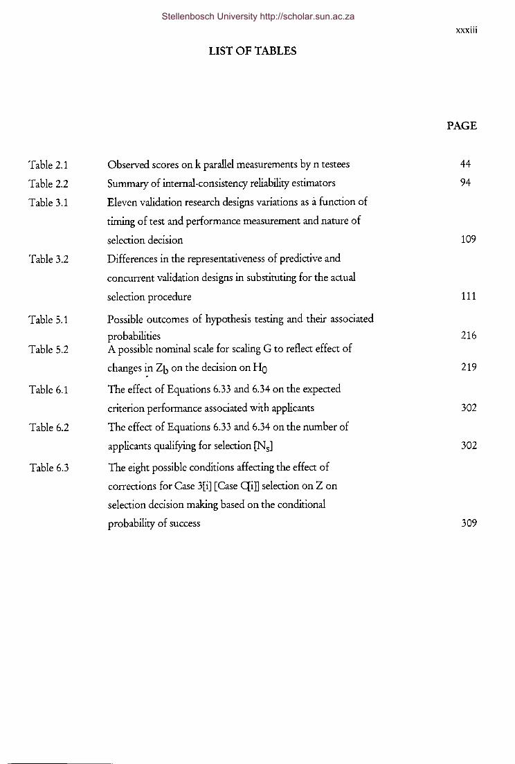
LIST OF TABLES
PAGE
Table 2.1 Observed scores on k parallel measurements by n testees 44
Table 2.2 Summary of internal-consistency reliability estimators 94
Table 3.1 Eleven validation research designs variations as a function of
timing of test and performance measurement and nature of
selection decision 109
Table 3.2 Differences in the representativeness of predictive and
concurrent validation designs in substituting for the actual
selection procedure 111
Table 5.1 Possible outcomes of hypothesis testing and their associated
probabilities 216 Table 5.2 A possible nominal scale for scaling G to reflect effect of
changes in Zb on the decision on Ho 219
Table 6.1 The effect of Equations 6.33 and 6.34 on the expected
criterion performance associated with applicants 302
Table 6.2 The effect of Equations 6.33 and 6.34 on the number of
applicants qualifying for selection [N sJ 302
Table 6.3 The eight possible conditions affecting the effect of
corrections for Case 3[i] [Case Qi] selection on Z on
selection decision making based on the conditional
probability of success 309
Stellenbosch University http://scholar.sun.ac.za
CHAPTER1
INTRODUCTION, RESEARCH OBJECTIVE AND OVERVIEW OF THE STUDY
The purpose of the introductory chapter is to present a reasoned exposition of the necessity and
significance of the envisaged research and to provide a formal statement of the research objective. In
-~ssen_ce_ i_£i_s -~gt!~~th~t~<l:<:fi_?~n~lEe~s~re~_ent ar:<!_!~ the~ry p_:ovide an ~~~eg'!~te conc_:ptu~ -~:am.!~~~_§"om w!llch to as~ess the p_ractical usefulness of p_sychometric tests in selection decisions.
Selection utility analysis theory in contrast provides a more appropriate framework for analysing,
describing and explaining selection decisions in terms of their consequences. Although utili!Y analysis
__theqry_clearly shows the deficiencies inherent in defining payoff resulting from a selection procedure
solely in terms of the validity coefficient [or translations thereof], it still acknowledges the pivotal role
of the validity coefficient in the development and evaluation of selection strategies. Effective selection
strategies are possible to the extent that the consequences of a selection decision relevant to the person
making the selection decision are systematically related to the information used to make the decision.
Relevant information therefore constitutes a necessary.I..r although not sufficient, prerequisite to develop
an effective, efficient and defendable selection strategy. The fundamental notion of a linear
relationship between a predictor [or a linear composite of predictors] and a criterion expressed in terms
of the parameters [i.e .. regression parameters and correlation coefficient] of the general linear model
[GLM] thus forms a basic building block in all utility analysis models. The implicit requirement made
by the GLM applied to selection problems is that the context in which the selection~_strategy will
~e?~all~ be applie_d ~ould be mirrored in the context in which the selection strat~~ is develol'ed and
evaluated/trial-tested. This would firstly require the dependent variable being regressed on the
weighted composite of predictors to be the latent criterion and not an operational indicator of it
attenuated by measurement error. A further requirement is that the parameters of the GLM are
estimated from a representative sample from the actual applicant population [i.e. the range of scores
observed in the sample should correspond to the range of scores for which the predictor will eventually
be used]. The observed criterion variable does, however, contain measurement error and a
representative sample from the applicant population is normally not available. The attenuating effect of
both these influences on the actual, empirically derived, validity coefficient is well recognised, and
procedures to derive a correlation corrected for attenuation due to the unreliability of the criterion
and/ or restriction of range are generally available [Ghiselli, Campbell & Zedeck, 1981; Lord & Novick,
1968]. If ·these corrections for attenuation due to the unreliability of the criterion and/ or restriction of
range would, however, be restricted to the validity coefficient only, relatively little would be gained in as
far as the decision function, the different definitions of payoff permitted by utility analysis theory and
the statistical audit of the fairness of the selection strategy would remain unaffected. The actual
practical usage of the selection procedure, as well as any evaluative conclusion on the usefulness of the
selection procedure, would therefore not be affected. This, however, raises the question whether
Stellenbosch University http://scholar.sun.ac.za
2
corrections for attenuation due to the unreliability of the criterion and/ or restriction of range should be
extended to the GLM based decision function, the different definitions of payoff permitted by the
utility analysis theory or the statistical audit of the fairness of the selection strategy, and if so, what the
effect of these corrections would be. The question regarding the advisability of correcting for the
unreliability of the criterion and/ or restriction of range in essence hinges on the probability that such
corrections would change decisions, the consequences of these changed decisions and the cost of
obtaining the reliability estimates needed to implement the corrections.
1.1 INTRODUCTION
Organisations do not constitute natural phenomena but rather man made phenomena and therefore
exist, in as far as human behaviour is motivated, goal directed behaviour, for a definite reason and with
a specific purpose. The human resource function justifies its inclusion in the family of organisational
functions through its commitment to contribute towards organisational goals. Ahnost all definitions of
human resource management formally and explicitly profess this commitment. At the same time,
however, insufficient effort is devoted to explicitly delineate these organisational goals in abstract terms
with sufficient clarity. Although the general motivation underlying interventions launched under the
banner of the human resource function [e.g. human resource selection] is thus clear, inadequate
explication of the primary organisational goal still has the effect of obscuring the logic in terms of
which the human resource function should be able to justify its assertion that it contributes towards
organisational goals. Consequently it becomes very difficult to infer, through a reasoned argument, the
appropriate criteria in terms of which human resource intervention [e.g. human resource selection]
should be evaluated.
In order to be instrumental in the satisfaction of the multitude of needs of society, organisations have
to combine and transform scarce factors of production into products and services with maximum
economic utility. The organisation is thereby confronted with a choice of alternative utilisation
possibilities regarding the limited factors of production it has access to. The organisation is guided in
this choice by the economic principle, which commands, on behalf of society, the organisation to attain
with the lowest possible input of production factors the highest possible output of need satisfying
products and/ or services. The organisation [in a capitalistic system] complies with the demand of the
economic principle because such compliance enables it to maximise its profits. The motivation for the
organisation to serve society through the efficient production of need satisfying products and/ or
services thus lies in the opportunity to utilise the capital it has to its disposal, via economic activities
directed at the creation of need satisfying products and/ or services, for its own benefit. In order to
have an optimal exploitation of this opportunity, however, profitability maximisation must be
Stellenbosch University http://scholar.sun.ac.za
3
designated as the primary organisational goal. The primary objective for the organisation thus is the
maximisation of the profit earned over a particular period relative to the capital used to generate that
profit. Specifically this objective refers to the rate of return on equity [Rademeyer, 1983], that is profit
[expressed as a percentage] earned on capital of ordinary shareholders. By subscribing to this principle
the organisation thus commits itself to the maximisation of the value of the organisation for its owners
[shareholders] as it manifests itself in the price of its share on the stock exchange [in the case of listed
companies] and the magnitude of dividends declared [dark, Hindelang & Prichard, 1984; Levy &
Samat, 1994; Lumby, 1994; Rademeyer, 1983]. Financial decisions, especially decisions regarding the
appropriation of capital, are guided by the quest to add value to the organisation. Therefore, in order
to justify the investment of capital in any project in terms of the quest to add value to the organisation,
the expected return on the investment, or the expected cash inflow generated by the project, should
exceed the amount initially invested in the project. In estimating the rationality of a contemplated
investment the time value of money [the fact that cash inflows occur over the lifetime of the project]
must be taken into account as well as the risk associated with the investment [Levy & Sarnat, 1994].
In order to actualise the primary objective of the organisation a multitude of mutually coordinated
activities need to be performed which can be categorised as a system of inter-related organisational
functions. The human resource function represents one of these organisational functions. The human
resource function aspires to contribute towards organisational objectives through the acquisition and
maintenance of a competent and motivated work force, as well as the effective and efficient utilisation
of such a work force [Crous, 1986]. The importance of human resource management flows from the
basic premise that organisational success is significantly dependent on the quality of its work force and
the way the work force is utilised and managed. Labour constitutes a pivotal production factor due to
the fact that the organisation is managed, operated and run by people. Labour is the life giving
production factor through which the other factors of production are mobilised and thus represents the
factor which determines the effectiveness and efficiency with which the other factors of production are
utilised [Marx, 1983]. The management of human resources is, however, complicated by the intricate,
and to a certain extent enigmatic, nature of working man as the carrier of labour as production factor.
This leads to the basic premise that credible and valid theoretical explanations [i.e. social science theory]
for the different facets of the work behaviour of working man constitute a fundamental and
indispensable, though not sufficient, prerequisite for efficient and equitable human resource
management.
Industrial/ Organisational Psychology embodies the conviction that, in spite of the extreme complexity
of human behaviour, regularities underlying the work-related behaviour of working man can be
unraveled and explained in terms of a nomological network of constructs [i.e. theory]. According to
Veldsman [1986] Industrial/Organisational Psychology is the behavioral science directed at the
psychological explanation of the work-related behaviour of working man. Industrial/Organisational
Stellenbosch University http://scholar.sun.ac.za

4
Psychology derives the fundamental reason for its existence from the potential "therapeutic" value
[Mouton & Marais, 1985] of valid social science theory. Industrial/ Organisational Psychology would
concede that perfect understanding and complete certainty regarding the principles governing the work
behaviour of man represents an unattainable ideal. Industrial/ Organisational Psychology would,
however, still contend that sufficiently comprehensive approximations of reality can be achieved
through a scientific methodology [therein lies in part the relevance of I/0 Psychology's commitment to
the scientific method of inquiry] to be of significant relevance to practical human resource decisions
[Milkovich & Boudreau, 1994; Mouton & Marais, 1985].
To the extent that Industrial/ Organisational Psychology can produce credible and valid theoretical
explanations for the different facets of the work behaviour of working man, an opportunity exists to
derive, through deductive inference, practical human resource interventions designed to affect either
employee flows or employee stocks [Boudreau, 1991; Milkovich & Boudreau, 1994]. Interventions
designed to affect employee flows attempt to change the composition of the work force by adding,
removing or reassigning employees [e.g. through recruitment, selection, turnover, or internal staffing]
with the expectation that such changes will manifest in improvements in work performance. In
contrast interventions designed to affect employee stock attempt to change the characteristics of the
existing work force in their current positions or the work situation itself [e.g. through training,
performance feedback, compensation or job redesign]. The expectation is that such changes will
manifest in improvements in work performance [Boudreau, 1991]. Improvements in work
performance are affected through increases in work force quality which in turn are brought about by
the aforementioned two types of human resource interventions. Improvements in work performance
as such would however not constitute sufficient evidence to justify the intervention that affected these
improvements. Given that the human resource function's inclusion in the family of organisational
functions is justified through its commitment to contribute towards the primary organisational
objective of maximising the value of the organisation for its owners, it logically follows that all
interventions initiated by the human resource function should, in the final analysis, also be evaluated
with the yardstick of profitability. Babbel, Stricker and Vanderhoof [1994, p. 3] come to a similar
conclusion with regards to insurance managers:
One of the most basic tenets of modem financial theory is that managers should act in a manner consistent
with maximizing the value of owners' equity. While there are theoretical conditions under which this tenet
may not always apply, for practical purposes companies usually espouse it as a financial goal. If an insurer
accepts this maxim as a company goal, it follows that the firm should view the performance of insurance
managers and operatives in terms of whether this performance helps to promote higher firm value.
"------ -The design, implementation and operation of human resource interventions thus only make sense from
an institutional perspective if a satisfactory [appropriately discounted] return on the capital invested in
Stellenbosch University http://scholar.sun.ac.za
5
the intervention is achieved over the period in which the intervention generates its effect. There thus
rests an obligation on the human resource function to prove through appropriate financial indicators
[Boudreau, 1991; Cranshaw en Alexander, 1985] that its interventions do add value to the organisation
[Cascio, 1991b]. Furthermore it seems reasonable to contend that the only rational way the human
resource function can compete for limited capital on a more or less equal footing with the other
organisational functions is in terms of expected returns on capital invested [Cranshaw en Alexander,
1985]. The burden of persuasion rest particularly heavy on the human resource function due to its
general inability in the past to demonstrate its ability to contribute to bottom-line success [Cascio,
1991b]. In as far as the human resource function had neglected to meet this burden of persuasion, a
relative lack in stature, influence and recognition, in comparison to the other organisational functions,
seems hardly surprising [Cranshaw en Alexander, 1985; Gow, 1985; Sheppeck & Cohen, 1985]. Fitz
Enz [1980, p. 41] comments as follows in this regard:
Few human resource managers, even the most energetic, take the time to analyze the return on the
corporation's personnel dollar. We feel we aren't valued in our own organizations, that we can't get the
resources we need. We complain that management won't buy our proposals and wonder why our advice is so
often ignored until the crisis stage. But the human resources manager seldom stands back to look at the total
business and ask: Why am I at the bottom looking up?. The answer is painfully apparent. We don't act like
business managers, like entrepreneurs whose business happens to be people.
The question regarding the return on capital invested in human resource interventions should,
however, not be exclusively addressed to the human resource practitioner but should also be directed
to the industrial psychologist as behavioral scientist. Industrial/ Organisational Psychology studies the
behaviour of working man in an effort to try and uncover the principles governing work related
behaviour on account of the "therapeutic" value such insight offers. To the extent that it can be shown
that human resource interventions, deductively derived from Industrial/ Organisational theory, do [or
do not] add value to the organisation, crucial information is fed back to the [basic/academic] research
arena. Apart from the guidance value thereof, such feedback, in the final analysis, constitutes the
decisive criterion in terms of which Industrial/ Organisational Psychology [like its human resource
management counterpart] should judge the extent to which it succeeds in its professed mission.
Human resource interventions can, however, not be evaluated solely in terms of the return on capital
invested in the intervention, since such interventions not only impact on the primary organisational
objective of maximising the value of the organisation for its owners. Human resource interventions
also impact on the psychological, physical and social wellbeing of current and prospective employees.
Human resource interventions not only have an institutionai payoff, but also an individual payoff.
Equal access to human resource intervention opportunities for all current and aspirant employees
would, from an institutional perspective, be considered irrational since it would nullify any institutional
Stellenbosch University http://scholar.sun.ac.za
6
payoff that could otherwise have been derived from such interventions. Individual employees will,
therefore, unavoidably derive differential benefit from human resource interventions. Because of the
disparate impact of human resource interventions it becomes imperative that the fairness or justice of
such actions be assessed so as to ensure equitable human resource practices [Singer, 1993].
Human resource interventions therefore impact either positively or negatively on the financial position
of the organisation and on the lives of the people that serve as its employees or aspire to do so. Two
basic criteria are thus implied in terms of which human resource interventions need to be evaluated,
IX namely efficiency and equity [Milkovich & Boudreau. Two stakeholders are furthermore thereby
implied, namely management, representing the [financial] interests of the owners, and labour and its
organised representatives. Should the human resource function be challenged by management and/ or
by organised labour to defend any intervention it would, therefore, have to lead evidence to show the
efficiency and equity of the disputed intervention. The extent to which the human resource function
would be able to establish the integrity of the challenged intervention would depend on the validity and
credibility of the evidence led in its defense. The validity and credibility of the verdict on the efficiency
an~ equity of an intervention in turn would largely depend on the methodology in terms of which the
evidence was generated. Therein lies part of the motivation for the commitment of
Industrial/ Organisational Psychology to the scientific method of inquiry.
1.2 PERSONNEL SELECTION
Selection, as it is traditionally interpreted, represents a critical human resource intervention in any
organisation in as far as it regulates the movement of employees into, through and out of the
organisation. As such selection thus firstly represents a potentially powerful instrument through which
the human resource function could add value to the organisation [Boudreau, 1983b; Boudreau &
Berger, 1985a; Cascio, 1991b; Cranshaw en Alexander, 1985]. Selection secondly, however, also
represents a relatively visible mechanism through which access to employment opportunities are
regulated. Because of this latter aspect selection, more than any other human resource intervention,
had been singled out for intense scrutiny from the perspective of fairness and affirmative action [Arvey
& Faley, 1988; Milkovich & Boudreau, 1994]. The aforementioned two basic criteria [efficiency and
equity] thus also apply to the evaluation of selection procedures [Milkovich & Boudreau, 1994]. The
quest for efficient and equitable selection procedures, however, if not left to chance but pursued in a
rational and judicious manner, necessitates a clear and comprehensive elucidation of all relevant factors
that affect these desired outcomes. Only if guided by a formal framework synthesising all relevant
selection parameters and the way these parameters interact, can diagnostic analyses/ psychometric
Stellenbosch University http://scholar.sun.ac.za
7
audits of selection procedures, motivated by the desire to improve the efficiency and equity of such
procedures, become a viable and worthwhile endeavor.
Decision theory seems to provide the most productive framework in which to cast the selection
problem so as to attain such a guidance system [Boudreau, 1991; Cascio, 1991b; Cronbach & Gieser,
1965; Huber, 1980]. Cronbach and Gieser [1965], in their seminal and pioneering publication,
vigorously advocated the inability of traditional measurement and test theory, due to its emphasis of the
instrument and precision of measurement, to provide an adequate conceptual framework from which
to assess the practical usefulness of tests in selection. In selection, or any other applied situation for
that matter, psychological tests essentially serve the purpose of providing information for decision
making. The focus thus should be on the quality of the decision making and not on the psychometric
properties of the test, although this should not be interpreted to mean that measurement and test
theory in the Gulliksen [1950] tradition are to be regarded as irrelevant and obsolete. Two general
decision-theoretic approaches towards selection can be differentiated [Schuler & Guklin, 1991]:
> a descriptive approach focusing on explicating the decision heuristics actually used
by decision makers; and
> a normative approach focusing on explicating a formal decision structure to be used
by decision makers as a decision aid [Huber, 1980] to compensate for their bounded
rationality [March & Simon, 1958] when considering alternative options.
Selection can be conceptualised in a normative decision-theoretic framework from either an operational
or strategic perspective. Thus the focus could be placed on the individuals about whom decision are
required or on the selection procedure itself.
Cascio [1991, p. 178], in an effort to establish the capacity of decision theory to provide a suitable
framework in which to cast the selection problem, clearly approaches selection from an operational
perspective when he asserts:
It should serve as some comfort to know that all personnel decisions can be characterized identically. In the
first place there is an individual about whom a decision is required. Based on certain information about the
individual [for example performance appraisals, assessment center ratings, a disciplinary report], decisions
makers may elect to pursue various alternative courses of action.
Cronbach and Gieser [1965, pp. 135-136], likewise, in their endeavor to point out the inadequacy of
traditional measurement theory as a conceptual vehicle to evaluate the usefulness of selection
instruments, operate from an operational perspective when they state:
Stellenbosch University http://scholar.sun.ac.za

The traditional theory views the test as measuring instrument intended to assign accurate numerical values to
some quantitative attribute of the individual. It therefore stresses, as the prime value, precision of
measurement and estimation. .... In pure science it is reasonable to regard the value of a measurement as
proportional to its ability to reduce uncertainty about the true value of some quantity. .... In practical testing,
however, a quantitative estimate is not the real desideratum. A choice between two or more discrete
treatments must be made. The tester is to allocate each person to the proper category, and accuracy of
measurement is valuable only insofar as it aids in this qualitative decision.
1.2.1 An Operational Perspective on Personnel Selection
8
When viewed from an operational perspective selection decisions can be characterised in terms of the
following structural elements [Cronbach & Gleser, 1965]:
~ a set of individuals about whom limited information is available
~ a set of decision options or treatments to which individuals have to assigned;
~ a decision function specifying treatment assignment contingent on information
about individuals;
~ a set of outcomes contingent on the assignment of individuals to specific treatments
described in terms of a multidimensional [composite] criterion; and
~ a utility scale on which the possible outcomes are evaluated.
Assuming that a selection quota 1s m force, the task with which the selection decision maker is
confronted is in essence to identify a subgroup from the total group of applicants to allocate to the
accept treatment, based on limited but relevant information about the applicants. The subgroup,
furthermore, has to be chosen so as to maximise the average gain on the utility scale on which the
outcomes of decisions are evaluated. The utility scale/ payoff and the actual outcomes or ultimate
criterion [Austin & Villanova, 1992] are the focus of interest in selection decisions [Ghiselli, Campbell
& Zedeck, 1981]. These are, however, by definition not available at the time of the selection decision.
Under these circumstances, and in the absence of any [relevant] information on the applicants, no
possibility exists to enhance the quality of the decision making over that that could have been obtained
by chance. The only alternative to random decision making [other than not to take any decision at all],
would be to predict expected outcomes/ criterion performance [or expected utility] actuarially [or
clinically] from relevant, though limited, information available at the time of the selection decision.
Thus some substitute1 for the criterion is called for [Ghiselli, Campbell & Zedeck, 1981]. The only
information available at the time of the [fixed treatment] selection decision [Cronbach & Gieser, 1965]
1 Formally X, and therefore by implication E[YIX], could be considered a substitute for Y if and to the extent that lp[X,Y]I > 0 [p < 0.05] and if measures of X can be obtained at the time of or prior to the selection decision
Stellenbosch University http://scholar.sun.ac.za
9
that could serve as such a substitute would be psychological, physical, demographic or behavioural
information on the applicants. Such substitute information would be considered relevant to the extent
that the regression of the [composite] criterion [or corresponding utility scale values] on a weighted
[probably, but not necessarily, linear] combination of information explains variance in the criterion.
Thus the existence of a relationship, preferably one that could be articulated in statistical terms,
between the outcomes considered relevant by the decision maker and the information actually used by
the decision maker, constitutes a fundamental and necessary, but not sufficient, prerequisite for
effective and equitable selection decisions.
Two, and only two, options exist in terms of which an acceptable substitute for the criterion could be
found. In terms of the first option the job in question would be systematically analysed via one or
more of the available job analysis techniques [Gatewood & Feild, 1994] to identify and define the
behaviours that collectively denote job success if exhibited on the job. Substitute information would
then be obtained through low or high fidelity simulations of the job content. These simulations in a
selection context necessarily occur off the job and at prior to the selection decision. Such simulations
would elicit behaviour that, if it would in future be exhibited on the job, it would denote a specific level
of job performance. These behaviours are sometimes referred to as competencies [Saville &
Holdsworth Ltd, 1996]. If competencies, defined in this sense, are assessed off the job via some form
of simulation [in contrast to on the job via actual job performance] the resultant assessments combined
can be regarded as a predictor of the criterion and thus as a substitute for the criterion. If, however,
competencies, defined in the above interpretation of the term, would be assessed on the job via actual
job performance the resultant assessments combined would constitute criterion measures.
In terms of the second option the job in question would also be systematically analysed but now with
the purpose of inferring suppositious critical incumbent attributes, believed to be determinants of the
level of criterion performance that would be attained, from the description of the job content and
context. These critical attributes are unfortunately also sometim~s referred to as competencies
[Spangenberg, 1990] thereby creating a good measure of confusion, misunderstanding and discord in
contemporary psychometric debate. The presumed interrelationship between these hypothesised
determinants and the way they collectively combine in the criterion is postulated in a nomological
network or latent structure [Campbell, 1991; Kerlinger, 1986] as a complex hypothesis explaining
criterion performance in the job in question. These hypothesised determinants of criterion
performance, or a person centered subset thereof, could, to the extent that the tentative performance
theory is indeed valid, serve in combined form as a suitable substitute measure for the, still to be
realised, actual criterion scores. The way these hypothesised determinants of performance should be
combined is suggested by the way these determinants are linked in the postulated nomological network.
Stellenbosch University http://scholar.sun.ac.za
10
The extent to which effective substitute criterion measures are obtained through these two options
should be the subject of empirical validation investigations. This would establish the foundation for a
comprehensive argument in terms of which the actual use of any selection procedure could be justified
from the perspective of both efficiency and equity.
In the case of the first option, the fundamental question is whether a content [factorially] valid
description of the competencies are obtained through the simulation and, if so, whether this description
correlates statistically significant with an independently obtained construct valid measure of the ultimate
criterion [Austin & Villanova, 1992].
In the case of the second option, the fundamental question is whether a weighted linear [or even
possibly non-linear, depending on the directive emanating from the postulated nomological network]
combination of construct valid measures of the hypothesised determinants of performance significantly
explains variance in a construct valid measure of the ultimate criterion.
Clearly substantial differences exist between the logic underlying these two options in terms of which
substitute criterion measures are generated. Most relevant, is the fact that the second option
necessitates the explication of an underlying performance theoty whilst the first option can proceed
without any significant understanding as to why inter-individual performance differences exist. Both
arguments, however, maintain that effective, though not necessarily efficient, selection is contingent on
the identification of a substitute [in the form of a differentially weighted combination] for the ultimate
criterion which shows a statistically describable relationship with an operational measure of the ultimate
criterion. Both arguments, furthermore, contend that the same condition constitutes a necessaty,
though not sufficient condition to achieve fair or equitable employee selection. The extent to which
the substitute succeeds in representing the ultimate criterion is in both cases described by the validity
coefficient as a multiple correlation between a composite intermediate criterion and a weighted
combination of the indicators of performance [Ryy~]. A perfect correlation would imply that the
decision maker has a flawless understanding of the predictor-criterion latent structure [Campbell, 1991],
can obtain psychometrically flawless measures of all relevant constructs and thus could, with perfect
precision and complete certainty, infer values on the intermediate criterion from the combined
substitute measure. The decision maker would have a relative simple selection problem to contend
with if this would be the case because it would imply that he can, with complete certainty, anticipate the
actual outcomes for any applicant should such an applicant be accepted. For such a perfectly informed
decision maker there would be no unanticipated consequences and thus also no risk and no decision
errors. This is, however, never the case [March & Simon, 1958]. The situation the decision-maker has
to contend with is characterised by relevant, limited and psychometrically flawed information. Relevant,
limited and psychometrically flawed· information would thus imply the classic imperfectly correlated,
bivariate [linear, homoscedastic and normal] distribution of composite criterion and composite
Stellenbosch University http://scholar.sun.ac.za
11
predictor/substitute criterion scores [Boudreau, 1991; Campbell, 1991; Cronbach & Gieser, 1965].
This classic validity model forms the foundation of all selection procedures [Boudreau, 1991; Campbell,
1991]. The decision maker's lack of perfect understanding and complete certainty regarding the
principles governing the outcomes resulting from acceptance, combined with his reliance on fallible
information, thus denies him the possibility of anticipating selection outcomes with complete certainty.
His access to relevant but limited and psychometrically flawed information, however, still permits him the possibility of statistically describing the conditional distribution of outcomes. Thus the decision
maker can only base his decision whether to accept an applicant on the expected outcome conditional
on information on the applicant or, if a minimally acceptable outcome state can be defined, the
conditional probability of success [or failure] given information on the applicant. Alternatively, the
bivariate distribution could be converted into a contingency table through the formation of intervals on
both the predictor and the criterion. The resultant validity matrix [Cronbach & Gieser, 1965] or
expectancy table [Ghiseli, Campbell & Zedeck, 1981; Lawsche & Balma, 1966], indicating the
probability of a specific criterion state conditional on a specific information category, could then be
used as basis for decision-making. If one would, furthermore, be willing to assume the existence of a
cardinal utility scale on which outcomes can be evaluated, if not linearly, at least monotonically related
to the criterion scale, it becomes possible to translate the expected outcome to the expected payoff
conditional on information on the applicant. [Crocker & Algina, 1986; Cronbach & Gieser, 1965].
The embryonic question, from which a construct orientated [option-two] selection procedure 1s
ultimately conceived, asks with deceptive simplicity why differences in performance exist. Inability to
answer this question in terms of a valid performance theory effectively eliminates the possibility to
differentiate between better and poorer employment prospects. Unless one is willing to assess
suitability for employment through demonstration of competency in tasks corresponding to the critical
performance areas comprising the job in question [i.e. through simulations via a content orientated
approach] and thus can sidestep the question as to why performances differences exist. Attaching the
term ability to each critical performance area provides no satisfactory answer to this question but
simply creates the impression of explanation. This line of reasoning suggests the validation of a
selection procedure to be, in essence, a form of applied explanatory scientific research [Binning &
Barrett, 1989; Ellis & Blustein, 1991; Landy, 1986]. Landy [1986, pp. 1187-1188] supports this
assertion, by stating:
The validity analyst is cartying out traditional hypothesis testing. At least by implication, the hypothesis being
considered is of the folloWing form: People who do well on test X will do well on activity Y, or Y =f[X].
Investigators should not lose sight of the fact that validity studies are attempts to develop a theory of
performance that explains how an individual can [or will] meet the demands of a particular job.
Stellenbosch University http://scholar.sun.ac.za
12
This seemingly benign position, that the validation of a selection procedure should be viewed from a
scientific, theoty building and hypothesis testing perspective, has in fact a multitude of far reaching
implications. By adopting this position one, in essence, formally acknowledges three basic premises,
two of which were already alluded to in the preceding discussion, namely:
);> valid theoretical explanations for the different facets of the work behaviour of working
man constitute a fundamental and indispensable, though not sufficient, prerequisite for
effective and efficient human resource management interventions;
);> the validity of theoretical explanations for the different facets of the work behaviour of
working man depend on the quality and thoroughness of the theorising that, in reaction
to the research initiating [why] questions, bring forth the the<:>retical explanations; and
);> the credibility/validity of statements on the validity of theoretical explanations for the
different facets of the work behaviour of working man depend on the unassailableness
of the methodological argument in terms of which these statements are justified.
Thus, by adopting this research orientated stance, one unequivocally restores theorisation and
conceptualisation to their rightful place in the selection procedure development process [Binning &
Barrett, 1989; Campbell, 1991; McGuire, 1997]. More crucial, however, for the argument in question, is
the formal recognition that the credibility/validity of statements on the validity of explanations of the
basic form Y = f[X] depends on the scientific rationality of the methodological argument through which
such conclusions were arrived at. This in turn, clearly has important implications for the type of
evidence the human resource function should lead should it be summoned, either by management or
regulatory agencies, to defend its selection procedures in terms of its efficiency and equity respectively.
The ability of the human resource function to successfully defend its selection procedure, however, is
not only dependent on the credibility/validity of statements on the validity of the performance
hypothesis underlying the selection procedure. Apart from the fact that further utility and fairness
analyses are required to establish the efficiency and equity of a selection procedure, a more fundamental
issue to be considered first, is the extent to which the validation research evidence can be logically
transferred to the actual area of application. Both these issues naturally emerge as critical themes if the
concept of research design is formally introduced.
Research design, if more extensively defined than is usually the case [Kerlinger, 1986], refers to the plan
and structure of the entire investigative process [Kerlinger 1986; Mouton & Marais: 1985] so conceived
as to justify the actual application of the selection procedure. Internal and external validity constitute
two general criteria of research design [Campbell & Stanley, 1963; Kerlinger, 1986]. Due to the more
extensive meaning attached to the research design concept, a concomitantly more comprehensive
definition of internal validity, encompassing the conventional interpretation of the term [Campbell &
Stanley, 1963; Cook & Campbell, 1979], is also required. Internal validity is typically interpreted to
mean the confidence with which [between group or systematic] variance in the dependent variable of
Stellenbosch University http://scholar.sun.ac.za
13
interest can be attributed to the effect of one or more independent variables [Babbie, 1989; Cook &
Campbell, 1979]. A more encompassing term is, however, needed here to refer to the confidence with
which the latent structure postulated by the research hypothesis [and not the operational hypothesis]
may be regarded as corroborated by the research evidence marshaled in its support within the limits set
by the specific conditions prevailing at the time of the investigation. However, rather than willy-nilly
[and somewhat arrogantly] redefining Campbell and Stanley's [1963] concept of internal validity to
satisfy the current argument's need for a single, suitably encompassing, concept, the trilogy of statistical
design criteria introduced by Cook, Campbell and Peracchio [1991] are employed to represent the
pertinent considerations. Statistical conclusion validity, internal validity and construct validity [Cock,
Campbell & Peracchio, 1991] collectively determine the credibility/validity of statements on the validity
of the performance hypothesis underlying the selection procedure. The confidence with which the
latent structure postulated by the research hypothesis may be regarded as corroborated by the research
evidence marshaled by a validation study would, therefore, be threatened by;
~ the lack of inferential validity of the deductive argument in terms of which the
research hypothesis is operationalised, especially the construct [and/ or content]
validity of the measurement procedures referred to in the premises contained in the
argument [Mouton & Marais, 1985];
~ the extent to which the research design fails to controls variance, that is, the extent
to which the design fails to maximise experimental/ systematic variance, fails to
minimise error variance and fails to control extraneous variance [Campbell &
Stanley, 1963;Kerlinger, 1986]; and
~ the extent to which statistical power [Cohen 1977] is decreased.
If validation of a selection procedure is viewed from a scientific, theory-building and hypothesis testing
perspective, the preceding argument makes it painfully clear that the "stamp collecting" approach
[Landy. 1986, p. 1184], induced by the tripartite division of validity [APA, AERA & NCJvlE, 1985],
represents an unjustifiable and misleading practice. To paraphrase Guion [1980, p. 386], there exists
only one road, and not "three different roads, to psychometric salvation" within the context of
selection research. The validation of multiple inferences are required to scientifically justify the pivotal
tenet on which selection procedures are based [Binning & Barrett, 1989]. Landy [1986, pp. 1185-1188]
summarises the unificationist perspective on the validation of selection procedures as follows:
The labels rontent, construct, and criterion-relaud are not completely useless, nor are they interchangeable. They
had their use in 1954, and they have their value in 1986. However, their value is not as types of validity.
Instead, their value is in pointing out that there is more than one type of inference that can be made from a
test score. .... Aspects of validity cannot be easily separated from one another. Because the words cortmt,
criterion-relatal, and construct can be used as aids in discussion, one should not be seduced into thinking of those
Stellenbosch University http://scholar.sun.ac.za
words as standing for discrete and independent processes. Instead, the words simply represent parts of a
larger system that addresses the goal of hypothesis testing.
14
A validation design [interpreted in the wider sense of the term] with adequate statistical conclusion
validity, internal validity and construct validity constitutes a necessary, but not sufficient, requirement to
construct a rigorous argument, that would be able to successfully withstand intellectual onslaught,
should it be required in litigation. A second, very crucial, line of defense required to defend the core of
any selection procedure concerns the external validity of the validation design.
To a certain extent external validity represents a rather elusive concept to pin down with a satisfactory
constitutive definition. For the purpose of the present argument, external validity is interpreted to refer
to the degree of confidence with which the [internally valid] results of a specific empirical validation
study can be generalised [or transported] to a specific area of application [Cook & Campbell, 1979;
Stanley & Campbell, 1963]. Generalisation, furthermore, always represents a problematic endeavor,
because it entails a risky extrapolation beyond the specifics characterising the validation study [Cook &
Campbell, 1979]. Generalisation, or induction, can never be completely justified by the evidence
supplied by a validation study; strictly speaking generalisation beyond the limits set by the validation
study is not possible at all [Mouton & Marais, 1985; Stanley & Campbell, 1963]. Nevertheless, given
the applied nature of selection validation research, an attempt at generalisation is unavoidable.
According to Stanley & Campbell [1963] external validity is threatened by the potential specificity of the
demonstrated effect of the independent variable[ s] to particular features of the research design not
shared by the area of application. In selection validation research the effect of the [composite]
independent variable on the criterion is captured by the validity coefficient. The area of application is
characterised by a sample of actual applicants drawn from the applicant population and measured on a
battery of fallible predictors with the aim of "estimating their actual contribution to the organisation
[i.e. ultimate criterion scores] and not an indicator of it attenuated by measurement error" [Campbell,
1991, p. 694] from a weighted linear composite of predictors derived from a representative sample
from the actual applicant population. The question regarding external validity, in the context of
selection validation research, essentially represents an inquiry into the unbiasedness of the parametric
validity coefficient estimated from the sample statistic obtained through the validation study. The
parameter of interest is the correlation coefficient obtained when the sample weights derived from a
representative sample are applied to the applicant population and the weight~d composite score is
correlated with the criterion, unattenuated by measurement error, in the population [Campbell, 1991].
The preceding discussion clearly indicates the term "applicant population" to be of central importance
should a sufficiently precise depiction of the area of actual application be desired. The term "applicant
population", however, even if defined as the population to which a selection procedure will be applied,
still has an annoying impreciseness to it. A more unambiguous definition of the term, however,
Stellenbosch University http://scholar.sun.ac.za
15
depends on how the selection procedure would be positioned relative to any selection requirements
already in use [i.e. whether it would replace, follow on, or be integrated with current selection
requirements]. This issue, moreover, is linked to the question regarding the appropriate decision
alternative with which to compare the envisaged selection procedure when examining its strategic merit.
Further clarification of the term will consequently be attempted in the ensuing discussion on the
strategic evaluation of selection proced~res. In the context of selection validation research, given the
aforementioned depiction of the area of application, the following specific threats to external validity
could thus be identified [Campbell, 1991; Lord & Novick, 1968; Tabachnick & Fidell, 1989]:
~ the extent to which the actual or operationalised criterion contains random
measurement error;
~ the extent to which the actual or operationalised criterion is systematically biased;
i.e. the extent to which the actual criterion is deficient and/ or contaminated [Blum
& Naylor, 1968];
~ the extent to which the validation sample is an unrepresentative, biased, sample
from the applicant population in terms of homogeneity and specific attributes [e.g.
motivation, knowledge/ experience];
~ the extent to which the sample size and the sample size to number of predictors
ratio allow capitalisation on chance and thus overfitting of data.
The conditions listed as threats do all affect the validity coefficient [Campbell, 1991; Crocker & Algina,
1986; Dobson, 1988; Hakstian, Schroeder & Rogers, 1988; Lord & Novick, 1968; Mendoza &
Mumford, 1987; Messick, 1989; Olsen & Becker, 1983; Schepers, 1996]. Some consistently exert
upward pressure, others downward pressure and for some the direction of influence varies. It thus
follows that, to the extent that the aforementioned threats did operate in the validation study but do
not apply to the actual area of application, the obtained validity coefficient cannot, without formal
consideration of these threats, be generalised to the actual area of application. The obtained validity
coefficient thus cannot, without appropriate corrections, be considered an ·unbiased estimate of the
actual validity coefficient of interest. Campbell [1991, p. 701] consequently recommends that:
If the point of central interest is the validity of a specific selection procedure for predicting performance over
a relatively long time period for the population of job applicants to follow, then it is necessary to correct for
restriction of range, criterion unreliability, and the fitting of error by differential predictor weights. Not to do
so is to introduce considerable bias into the estimation process.
Information is obtained and analysed/ processed at a cost with the purpose of making a decision [i.e.
choosing between two or more alternatives] which results in outcomes with certain value to the
decision-maker. Additional information and/ or additional analyses of information could be considered
rational if it results in an increase in the value of the outcomes at a cost lower than the increase in value.
Stellenbosch University http://scholar.sun.ac.za
16
The foregoing argument thus implies that corrections applied to the obtained correlation coefficient are
rational to the extent that [Boudreau, 1991]:
);;> the corrections change decisions on the validity of the research hypothesis in that
they change the magnitude of either the validity coefficient, or the standard error of
the validity coefficient, or both [or at least the a priori probability of rejecting Ho
assuming Ho to be false];
);;> the change in decisions have significant consequences;
);;> the cost of applying the statistical corrections are low.
If the probability of these corrections changing the pre-correction conclusion on the validity of the
research hypothesis is small, and the value of the change in decision is less than the cost of
implementing the corrections, one could thus contend that very little justification actually exists for
these corrections.
The concept of external validity as used here should, however, not be confused with two closely
affiliated, but distinct concepts, namely generalisability theory [Cronbach, Gieser, Nanda & Rajaratnam,
1972] and validity generalisation theory [Schmidt & Hunter, 1977; Schmidt, Hunter, Pearlman & Hitsh,
1985]. Generalisability theory, as an extension of reliability theory, is a statistical theory on the accuracy
of generalisations from a testee' s observed score on some measure to the average score that person
would have received over all acceptable observations [Shavelson & Webb, 1991]. Validity
generalisation theory postulates, in contrast to the traditional situational specificity position, that
observed situational variability in test-criterion correlations can be explained in terms of statistical
artifacts and thus that criterion-related validity is generalisable across different situations [Messick,
1989]. The statistical artifacts normally considered by validity generalisation theory to contribute to
artifactual validity variance are sampling error, criterion unreliability, predictor unreliability, restriction
of range and criterion contamination [Duvenage, 1991; Messick, 1989;]. Validity generalisation theory
clearly also represents a manifestation of the Cook and Campbell [1979] concept of external validity. It
differs, however, from the argument developed here, in that it requires meta-analysis [Hunter, Schmidt
& Jackson, 1982] of extensive criterion-related validity data sets, generated by individual validation
studies, to estimate the mean and standard deviation of the true validity distribution. The present
argument, on the other hand, focuses on the removal of artifactual effects in the individual validation
study result. Neither an extreme validity generalisability position nor an extreme situational specificity
position is, however, probably warranted. The two positions should thus not be pitted against each
other, but should rather be viewed as interdependent, mutually complementary, approaches [Messick,
1989; Raudenbush & Bryk, 1985]. Although an extreme validation generalisability position would
render local validation studies questionable, the extensive benefits afforded by such studies, point to the
necessity and pertinence of local validation studies in conjunction with validity generalisation research
[Messick, 1989; Raudenbush & Bryk, 1985; Schmidt, Hunter, Pearlman & Hirsh, 1985].
Stellenbosch University http://scholar.sun.ac.za
17
Once the latent structure, postulated by the research hypothesis as foundation for the selection
procedure, is adequately corroborated by the research evidence marshaled in its support and the results
can, following appropriate corrections, be generalised [or transported] to the specific area of
application, attention shifts to the selection strategy.
A selection strategy or selection decision function refers to an explicit or implicit rule dictating,
conditional on available information, whether an applicant should be terminally rejected or accepted, or
whether and what further information should be collected [Cronbach & Gieser, 1965; Gatewood &
Feild, 1994; Muchinsky, 1983]. A selection strategy, in essence, consists of conditional probabilities
[normally 0 or 1, but not necessarily] stating the probability of each treatment/ decision, conditional on
information on the applicant. A selection strategy thus could be enunciated in terms of a strategy
matrix [Cronbach & Gieser, 1965], prescribing, or describing, through conditional probabilities
associated with different information categories, how applicants should be, or are, assigned to the
different possible treatments.
The nature of the selection strategy depends on the manner in which multiple selection information is
combined for decision-making [that is, whether compensation will be permitted, whether multi-stage
sequential testing will be employed] and whether quotas are in force. Whether compensation is
permitted would impact on the number of ways [Coxon, 1982; Schiffman, Reynolds & Young, 1981]
comprising the strategy matrix, restricting it to two if compensation is allowed. AssUming an
information x decision format, multi-stage sequential testing would increase the number of strategy
matrices from one to the number of stages and would increase the number o( columns from two to
three in all the matrices except the final one. Quotas, in tum, would impact on the conditional
probabilities contained in the strategy matrix. The following [actuarial] selection strategies are typically
distinguished [Gatewood & Feild, 1994; Milkovich & Boudreau, 1994]:
~ multiple regression strategy [single-stage, compensation allowed];
~ multiple cutoff strategy [single stage, limited compensation];
~ multiple hurdle strategy [multi-stage, no compensation;
~ profile comparison strategy [single stage, no compensation]; and
~ hybrid strategies.
A [multiple] regression strategy was implicitly assumed in the preceding argument and will henceforth
be formally assumed. A two-way strategy matrix is thus assumed. The information categories in such a
strategy matrix would consist of class intervals formed on either the expected criterion score scale or
the conditional probability of success scale. The nature of the cell entries in the strategy matrix would
depend on whether a quota is in force and/ or the aspiration level of the decision maker as it manifests
Stellenbosch University http://scholar.sun.ac.za

18
itself in the specification of a minimally acceptable criterion score and/ or conditional probability for
success.
Earlier it was argued that the obtained validity coefficient cannot, without appropriate corrections, be
considered an unbiased estimate of the actual validity coefficient of interest. It was thus argued that the
validity coefficient should be corrected for restriction of range, criterion unreliability, and the fitting of
error by differential predictor weights before being transported to the area of application. If these
corrections would be applied, the validity coefficient would be adjusted, but that still leaves the
information contained in the strategy matrix unaffected. The decision strategy actually applied for
decision-making is thus still the one derived from a simulated application, which, however, is not fully
representative of the actual application. This, however, begs the question whether this matters; that is,
do the characteristics in terms of which the context in which the decision strategy is actually applied
differ from the context in which it was developed in any way affect the decision strategy, and if so, in
which way(s]. If the considerations underlying the corrections previously applied to the correlation
coefficient do in fact also affect one or more of the facets of the decision strategy, corrections to the
decision rule would then be required. That would, however, in tum bring the following question to the
fore again:
~ would such corrections change decisions on employment applicants?; and if so
~ what would the value of the consequences of the change in decisions be?; and
~ how would the cost of the corrections compare to the value of the changed
decisions affected by the corrections?.
Again, as previously, one could contend that such corrections applied to the decision rule do in fact
serve no practical purpose if they do not change the actual decisions on applicants for employment or
do so at a cost exceeding the value of the change in decisions.
It should be kept in mind that all the evidence required to develop and justify a selection procedure in
terms of efficiency and equity is obtained in an artificial, simulated environment. The contention is
thus, that the concern with external validity cannot logically be restricted to the validity coefficient only,
but should extend throughout the whole argument in terms of which a selection procedure is
developed and justified.
The all-important, but too often grossly neglected, question regarding the justifiability of a selection
procedure shifts the attention from the development and operation of a selection strategy to the
evaluation thereof. Evaluation of human resource interventions generally serve two purposes, namely
[Rossi & Freeman, 1985; Weiss, 1972]:
Stellenbosch University http://scholar.sun.ac.za
19
~ to determine the extent to which the intervention in question did serve the purpose
it was designed for and in the manner intended, and in so doing, justify its current
and continued usage; and
~ to provide the diagnostic feedback needed to improve the intervention's ability to
serve the purpose it was designed for.
According to Rossi and Freeman (1985, p. 19] evaluation research refers to:
the systematic application of social research procedures in assessing the conceptualization and design,
implementation, and utility of social intervention programs. In other words, evaluation research involves the
use of social research methodologies to judge and to improve the planning, monitoring, effectiveness, and
efficiency of health, education, welfare, and other human service programs.
In all fairness to Rossi and Freeman (1985] it should be stated that they probably did not have selection
procedures in mind when they referred to social intervention programs. Nonetheless, a wider
interpretation of social intervention programs could legitimately include human resource selection
procedures.
The rather comprehensive definition offered by Rossi and Freeman (1985] endorses the posltlon
enunciated earlier that the empirical investigation of the theoretical base of a selection procedure, so as
to establish its validity, constitutes an important and necesscuy, but not sufficient, first phase of
evaluation. A second phase of evaluation concerns the extent to which the actual decision-making
practice departs from the instructions contained in the strategy matrix. If the decision maker should,
contrcuy to the prescription of the selection strategy, differentiate between applicants falling in the same
information category, based on additional clinical information, the chances are, despite strong personal
convictions to the contrary, that the effectiveness and efficiency of his decision making would thereby
be impaired [Cronbach & Gieser, 1965; Gatewood & Feild, 1994; Meehl, 1954; Tenopyr, 1983]. The
third phase of evaluation concerns the actual impact of the selection procedure. All three phases of
evaluation, and not only the impact evaluation phase, are necesscuy to construct a sound justification
for a selection procedure and all three phases afford valuable feedback to improve on the performance
of a selection intervention.
1.2.2 A Strategic Perspective on Personnel Selection
Shifting the focus to the evaluation of impact results in a concomitant shift in the perspective from
which selection is conceptualised in a normative decision-theoretic framework. A selection strategy
Stellenbosch University http://scholar.sun.ac.za
20
serves the purpose of guiding numerous decisions about applicants made by human resource managers
and therefore should be evaluated by "its total contribution when applied to a large number of
decisions" [Cronbach & Gieser, 1965, p. 23]. Thus the focus should now be placed on strategic
decisions about selection procedures rather than on operational decisions about individual applicants
[Boudreau, 1991; Cascio, 1991b]. The decision options under consideration are therefore not
individual applicants, but rather different possible procedures or strategies that could be used to assign
applicants to treatments [Boudreau, 1991; Cronbach & Gieser, 1965].
Multi-attribute utility [MAU] theory represent a decision theoretic approach directed at an analysis of
the usefulness and desirability of decision options under conditions of uncertainty, multiple conflicting
objectives, and costs and benefits accruing to various stakeholders [Huber, 1980; Keeny & Raiffa,
197 6]. As a specific exponent of the latter approach, selection utility models are characterised by the
following structural elements [Boudreau, 1991; Boudreau, 1989]:
);;> a set of decision options that represent the alternative procedures or strategies
under consideration;
);;> a set of attributes affected by the decision, reflecting the characteristics of the
outcomes considered relevant by the decision maker and pertinent constituencies;
);;> a utility or payoff scale reflecting the value of each attribute to the decision maker;
);;> a payoff function, reflecting the weight assigned to each attribute and the rule in
terms of which the differently valued attributes are combined to estimate the total
utility of each option under consideration; and
);;> a set of parameters characterising the decision situation in which the selection
strategy will be used.
The option set most often considered by selection utility models comprises the use of a specific battery
of selection instruments under the directive of a specific selection strategy versus random selection
[Boudreau, 1991; Taylor & Russell, 1939]. Defining random selection as the baseline implies the value
of selection procedures to be adequately captured by the extent to which it improves selection
efficiency over and above, that which would have been achieved by chance alone. According to
Cronbach and Gieser [1965] such reasoning can easily lead to overoptimistic estimates of selection
utility if proper care is not taken in delineating the appropriate decision alternative with which to
compare the selection procedure in question. The important point to recognise is that if the application
of the selection procedure were impossible the decision maker need not fall back on chance decision
making, but would base his decisions on whatever prior information is available. The decision option
with which the envisaged selection procedure should be compared is thus the best a priori strategy
[Cronbach & Gieser, 1965]. How this comparison should be made, and simultaneously, as was
indicated earlier, the meaning afforded to the term "applicant population", depends on the way the new
Stellenbosch University http://scholar.sun.ac.za
,-~---------------------------------------------,
21
selection procedure is positioned relative to the selection requirements already in use. Cronbach and
Gieser [1965] identify the following three possibilities:
~ all selection requirements currently employed will continue to be used for pre
screening, and thus the envisaged strategy following on pre-screening should be
compared to the existing strategy [applicant population represented by pre-screened
applicants];
~ the new selection procedure will replace all current selection requirements, and thus
the two strategies should be compared [applicant population represented by
unscreened applicants]; or
~ the new procedure and current selection requirements will be integrated to produce
information for selection decision making, and thus the combined strategy should
be compared to the existing strategy [applicant population represented by
unscreened applicants].
Given a set of decision options, selection utility models specify an array of attributes in terms of which
the outcomes generated by any option would be described [Boudreau, 1991; Keeny & Raiffa, 1976].
Cronbach and Gieser [1965, p. 22] point to the need for multiple descriptors when characterising the
attribute domain by supplying the following, somewhat vague, definition:
all the consequences of a given decision that concerns the person making the decision [or the institution he
represents].
An exhaustive description of all the possible consequences resulting from a selection decision would be
so voluminous as to render any selection utility model useless as a practical decision aid. Thus, like any
other type of model, selection utility models have to simplify reality by omitting some lesser important
attributes. The attributes that should be retained are those most closely aligned with the decision
objective[s]. Milkovich & Boudreau [1994] identify two general categories of human resource
objectives, namely efficiency and equity, that could serve as beacons to guide the nomination of
attributes for inclusion in the salient attribute set. Efficiency related attributes are those outcome
characteristics that affect the organisation's ability to maximise output while minimising inputs. Equity
related attributes, in contrast, are those outcome characteristics that affect the fairness of the selection
procedure [Boudreau, 1991; Milkovich & Boudreau, 1994]. A small set of efficiency related attributes
seem to have dominated selection utility conceptualisations. Boudreau [1991, p. 628] contends that at
least three basic attributes should be considered to ensure an adequate selection utility model:
~ "Quantity - the number of employees and time periods affected by the
consequences of program options
~ Quality - the average effect of the program options on work force value, on a
per-person, per time-period basis
Stellenbosch University http://scholar.sun.ac.za

22
);> Cost- the resources required to implement and maintain the program option"
The third component of a selection utility model is a set of utility or payoff scales for each attribute,
established with the purpose of quantifying the level of each attribute, so as to articulate the decision
maker's satisfaction with the various attributes of the outcomes that could possibly be obtained. Some
abstract scale of utility might be employed for this purpose on which decision-makers subjectively scale
their evaluation of the different outcome attributes. This would, however, ignore the need to translate
the consequences of selection procedures into the everyday fmancial language of line management
[Cascio, 1991b; Cranshaw & Alexander, 1985; Gow, 1985; Sheppeck & Cohen, 1985]. Consequently
the quantity attribute is usually expressed in person-years while the cost attribute is usually measured in
an appropriate monetary unit [Boudreau, 1989]. In the case of the quality attribute, general consensus
exists that the appropriate scaling unit for this attribute should be dollars [that is, rand-cent] per person
year, although considerable disagreement still exists on what these values actually should reflect. Some
form of clarity, however, emerges if it is argued that human resource selection procedures provide
economic benefit to organisations through their ability to enhance the quality of the work force
employed [Boudreau, 1991]. The increase in work force quality, in turn, manifests itself in increased
work performance, which in turn manifests itself in improved output [Binning & Barrett, 1989;
Campbell, 1991]. How the organisation capitalises on such quality enhancement depends on how it
affects performance and eventually output. Both performance and output are multidimensional
concepts, and improvements in the quality of employees can manifest itself in increases in performance
and output in any one dimension, or combination of dimensions. At least three inter-related output
dimensions should be taken into account, namely [Boudreau, 1989; Boudreau, 1991]:
);> quantity of production or output;
);> quality of production or output; and
);> production cost.
This would then logically imply that organisations could derive economic benefit through enhanced
labour force quality, brought about by improved human resource selection [or any other human
resource intervention for that matter], by channeling the increased labour capability into either
[Boudreau, 1991 ]:
);> an increase in the quantity of production, and/ or;
);> an increase in the quality of production and/ or;
);> a reduction in production costs.
A utility scale for the quality attribute should thus be considered appropriately defined, if such a
definition could reflect changes in any one, or combination, of the aforementioned output dimensions.
At least three different interpretations of the payoff scale for the quality attribute seem to exist in
selection utility applications [Boudreau, 1991]:
);> payoff interpreted as cost reduction;
);> payoff interpreted as increased value of output or revenue; and
);> payoff interpreted as increased profits.
Stellenbosch University http://scholar.sun.ac.za
23
Only the profit interpretation of quality payoff encompasses all three output dimensions. This should,
however, not lead to the conclusion that the other two interpretations are totally without merit. The
applicability of the other two interpretations depends on the manner in which the organisation uses
qualit)r improvements brought about by improved selection strategies. Furthermore, a revenue based
interpretation of quality utility could still in the end deliver a profit based total utility estimate for the
option under consideration, by incorporating the cost output dimension in the payoff function
[Boudreau, 1991]. The measurement of utility in general, but particularly the utility associated with the
quality attribute, represents the Achilles' heel of selection utility analysis theory [Cronbach & Gieser,
1965]. This controversial theme will be discussed subsequently. ·
The fourth component of a selection utility model is the payoff function reflecting the weight assigned
to each attribute and the rule in terms of which the differently valued attributes are combined to
estimate the total utility of each option under consideration [Boudreau, 1989; Boudreau, 1991]. The
payoff function in essence creates the common value base needed to compare options in terms of their
ability to realize the decision objective. Such a common value base should, however, be related to the
decision objective and should be expressed in the same metric as the objective [Lumby, 1994]. The
payoff function applicable to selection utility models, should thus, given the fundamental position
enunciated in the introductory section of this chapter, be derived from the primary organisational
objective of profitability maximisation. Therefore, a specific selection strategy should be evaluated in
its totality by its contribution to profit earned over a particular period relative to the capital used to
generate that profit. To justify the investment of capital in a selection procedure in terms of the quest
to add value to the organisation, the expected cash inflow, appropriately discounted, generated by the
procedure, should therefore exceed the financial resources required to start-up and run the
intervention. Boudreau [1991, p. 629] proposes the following basic structure:
The payoff function may be considered a variant of the cost-volume-profit models used in other managerial
decisions to invest resources. The utility of an HRM program option is derived by subtracting cost from the
product of quantity times quality, with the program exhibiting the largest positive difference being preferred.
To restrict the payoff function to this basic form would, however, leave the decision-maker with
insufficient evidence to adequately evaluate and compare selection strategy alternatives. The
fundamental problem with the basic quality times quantity minus cost conception of overall payoff lies
in its disregard of the following relevant considerations [Lumby, 1994; Crenshaw & Alexander, 1985;
Boudreau, 1991; Levy & Sarnat, 1994]:
>- the time value of capital;
>- taxat10n;
>- variable costs;
>- multiple cohort effects; and
Stellenbosch University http://scholar.sun.ac.za
24
;;.. risk.
Thus the basic payoff function should be extended to reflect these considerations [See chapter 7].
The fifth and final component of a selection utility model is a set of parameters characterising the
situation in which the selection strategy is applied. The parameters of interest are those describing the
marginal criterion and composite predictor distributions for the applicant population. Of specific
interest is the proportion of applicants falling above the hiring cutoff on the composite predictor, or
the selection ratio [SR], and the proportion of applicants who would be successful if selection would
occur without the envisaged selection strategy, or the base rate [BR] [Milkovich & Boudreau, 1994;
Taylor & Russell, 1939]. In the case of restricted selection [i.e. a selection quota is in force], the
selection ratio is determined by the number of vacancies relative to the number of applicants. In the
case of unrestricted selection, however, the critical predictor cutoff, the mean and the standard
deviation of the composite predictor distribution determine the selection ratio. The base rate is a
function of the critical criterion cutoff defining minimum acceptable performance, the mean and the
standard deviation of the marginal criterion distribution. These parameters are influenced by an
intricate interaction between the aspiration level of the decision maker, the long-term effect of the
selection procedure, recruitment strategies and the dynamics of the labour market [Boudreau, 1991].
Selection utility models serve as reality simplifying conceptual frameworks designed as aids for
"describing, predicting and explaining the usefulness or desirability" of selection decision strategies,
"and analysing how that information can be used in decision making" [Boudreau, 1989, p. 228] aimed at
improving selection strategies. When viewed from a historical perspective, the evolution of selection
utility models present a fairly systematic progression from somewhat unsophisticated models to
detailed, complex and rather daunting contemporary models [Boudreau, 1991; Rauschenberger &
Schmidt, 1987]. The following utility models can be differentiated in terms of their interpretation of
utility I payoff:
;;.. payoff defined in terms of the validity coefficient;
;;.. payoff defined in terms of the success ratio;
;;.. payoff defined in terms of expected standardised criterion performance;
;;.. payoff defined in terms of a monetary valued criterion
Chapter 7 extends the preceding discussion by presenting a detailed analysis of the aforementioned
utility models.
Earlier it was argued that the obtained validity coefficient cannot, without appropriate corrections, be
considered an unbiased estimate of the actual validity coefficient of interest. It was, therefore, argued
that the validity coefficient should be corrected for restriction of range, criterion unreliability, and the
fitting of error by differential predictor weights before being transported to the area of application.
Stellenbosch University http://scholar.sun.ac.za
25
Furthermore it was contended that the concern with external validity cannot logically be restricted to
the validity coefficient only, but should extend throughout the whole argument in terms of which a
selection procedure is developed and justified. It was thus argued that if these corrections would be
applied to the validity coefficient, the effect thereof on the selection strategy should therefore also be
examined. The same logic, however, would also apply to the different interpretations of the utility
concept. The question is thus firstly whether the statistical corrections for the attenuating effect of
criterion unreliability and/ or various forms of restriction of range would affect the different utility
estimates in terms of expected value and/ or estimate variability. Furthermore, should such corrections
have any effect on the utility estimates, a second question emerges, namely whether the expected utility
values and/ or the risk associated with a specific selection option change to such an extent that the
decision on the selection option is altered. The foregoing argument thus implicitly concedes that the
value of statistical corrections of the validity coefficient in the final analysis depends on [Boudreau,
1984; Boudreau, 1991]:
~ the probability that the corrections can change decisions on selection options;
~ the consequences of the changed decisions; and
~ the cost of applying the statistical corrections.
If the probability of such corrections changing the pre-correction choice of a selection option is small
and/ or the value of the change in selection option is less than the cost of applying the statistical
corrections, all other possible effects momentarily ignored, little, justification would actually exist for
these corrections from a practical perspective.
1.2.3 An Equity Perspective on Personnel Selection
Should the human resource function be summoned, either by management or regulatory agencies, to
defend its selection procedures, it would have to construct a reasoned justification based on the
efficiency and equity of the selection procedure [Guion, 1991; Milkovich & Boudreau, 1994]. The
different aspects that should be incorporated in the efficiency component required by such a
justification were examined in the preceding discussion. The equity component required in such a
defense has, however, been largely ignored up to now.
Human resource selection procedures represents a powerful instrument enabling the human resource
function to add value to the organisation by virtue of its ability to regulate the quality and quantity of
employees flowing into, through and out of the organisation. Human resource selection procedures
derive their ability to add value to the organisation from their capability to discriminate between
applicants in terms of attributes relevant to job performance. Selection measures are designed to
Stellenbosch University http://scholar.sun.ac.za
26
discriminate and in order to accomplish its professed objective it must do so [Cascio, 1991a]. However,
due to the relative visibility of the selection mechanism's regulatory effect on the access to employment
opportunities, the question readily arises whether the selection strategy discriminates fairly. Selection
fairness, however, represents an exceedingly elusive concept to pin down with a definitive constitutive
definition. The problem is firstly that the concept cannot be adequately defmed purely in terms of
psychometric considerations without any attention to moral/ ethical considerations. The inescapable
fact is that, due to differences in values, one man's foul is another man's fair. The problem is further
complicated by the fact that a number of different defmitions and models of fairness exist which differ
in terms of their implicit ethical positions and which, under certain conditions, are contradictory in
terms of their assessment of the fairness of a selection strategy and their recommendations on remedial
action [Arvey & Faley, 1988; Cascio, 1991a; Petersen & Novick, 1976]. The following three distinct
fundamental ethical positions can be identified [Hunter & Schmidt, 1976]:
);;> unqualified individualism - selection strategies are ethically legitimate if they utilise
all available means to maximise the correlation between Y and E[Y I X] and select
those applicants with the highest expected criterion performance;
);;> qualified individualism; - selection strategies are ethically legitimate if they select
those applicants with the highest expected performance but with the proviso that
race, gender, creed or ethnicity shall not be considered even if these factors are
related to performance [i.e. would have increased the correlation between Y and
E[Y I X] had they been included in the selection battery]; and
);;> a quota position - selection strategies are ethically legitimate if the proportional
composition of the labour market is reflected in the proportional composition of
the work force selected.
A fairness model, based on one of the aforementioned ethical positions [or a variant thereof], serves
the purpose of formalising the interpretation of the fairness concept. A fairness model thus permits
the deduction of a formal investigative procedure needed to assess the fairness of a particular selection
strategy should such a strategy be challenged to disprove a prima facie showing of adverse impact
[Arvey & Faley, 1988]. A variety of fairness models have been proposed [Arvey & Faley, 1988; Cascio,
1991a; Petersen & Novick, 1976]. These fairness models examine the effect of the selection decision
function on different subgroups contained in the applicant population by simulating the selection
process on a representative sample from the applicant population. Assuming an applicant population
consisting of two subgroups [7t1 and 1t2] such a simulation would render information on two bivariate
[normal] distributions characterised by the following parameters:
);;> a predictor mean [p,[X]], variance[cr2[X], symmetry [B1[XJ] and kurtosis [B2[X]];
);;> a criterion mean [J.t[Y]], variance [ cr2[Y]], symmetry [B1[Y] and kurtosis [B2[Y]J;
);;> predictor and criterion reliability coefficients [Pttx and PttY ];
);;> a validity coefficient [p[X,Y1
Stellenbosch University http://scholar.sun.ac.za
27
> a regression equation [E[Yi IXJ = a+BXi]with a specific intercept [a] and slope [B];
> a standard error of estimate [ cr[Y I X]];
> a critical criterion cutoff [Y cJ and a critical predictor cutoff [XcJ and thus a specific
base rate [BR=(a+c)/n], selection ratio [SR=(a+b)/n] and a specific relationship
between the number of true positives [a], true negatives [d], false positives [b] and
false negatives [ c ]; and
> utilities [U(Oj)] associated with the four possible selection outcomes [Oj].
The various fairness models attempt to define unfairness in terms of differences on one or more of the
aforementioned parameters across the subgroups [7t1 and 7t2] contained within the applicant
population. At least thirteen different selection fairness models can be distinguished [ Arvey & Faley,
1988; Cascio, 1991a; Petersen & Novick, 1976]. Only three of these models will be formally examined
in this study, namely:
> the regression or Cleary model;
> the equal risk or Einhorn-Bass model; and
> the constant ratio or Thorndike model.
Chapter 7 extends the preceding discussion by presenting a detailed analysis of the aforementioned
fairness models.
Earlier it was argued that the obtained validity coefficient cannot, without appropriate corrections, be
considered an unbiased estimate of the actual validity coefficient of interest. It was, therefore, argued
that the validity coefficient should be corrected for restriction of range, criterion unreliability, and the
fitting of error by differential predictor weights before being transported to the area of application.
Furthermore it was contended that the concern with external validity cannot logically be restricted to
the validity coefficient only, but should extend throughout the whole argument in terms of which a
selection procedure is developed and justified. It was thus argued that if these corrections would be
applied to the validity coefficient, the effect of these corrections on the selection strategy, the different
interpretations of the utility concept and the risk associated with different selection options should also
be examined. The further question now arises whether the finding/verdict of the various preceding
fairness models when applied to a specific selection strategy and their recommendations on remedial
action, if required, would be affected by these corrections for criterion unreliability and/ or restriction
of range. Again one would argue as before that the value of statistical corrections of the validity
coefficient in the final analysis depends on [Boudreau, 1984; Boudreau, 1991]:
> the probability that the corrections can change decisions on the fairness of a
selection strategy;
> the consequences of the changed assessments of the fairness of a selection strategy;
and
> the cost of applying the statistical corrections.
Stellenbosch University http://scholar.sun.ac.za
28
If the probability of such corrections changing the verdict on the fairness of a selection strategy is small
and/ or the value of the effect of a changed assessment of the fairness of a selection strategy is less than
the cost of applying the statistical corrections, all other possible effects momentarily ignored, little
justification would actually exist for these corrections, although from a logical-theoretical perspective
they might seem to be indispensable.
1.3. SUMMARY AND RESEARCH OBJECTIVES
Selection, as it is traditionally interpreted, represents a critical human resource intervention in any
organisation in as far as it regulates the movement of employees into, through and out of the
organisation. As such selection thus firstly represents a potentially powerful instrument through which
the human resource function could add value to the organisation [Boudreau, 1983b; Boudreau &
Berger, 1985a; Cascio, 1991b; Crenshaw & Alexander, 1985]. Selection secondly, however, also
represents a relatively visible mechanism through which access to employment opportunities are
regulated. Because of this latter aspect, selection, more than any other human resource intervention,
had been singled out for intense scrutiny from the perspective of fairness and affirmative action [ Arvey
& Faley, 1988; Milkovich & Boudreau, 1994]. Two basic criteria are thus implied in terms of which
selection procedures need to be evaluated, namely efficiency and equity [Milkovich & Boudreau, 1994].
The quest for efficient and equitable selection procedures requires periodic psychometric audits to
provide the feedback needed to iterate the selection procedure to greater efficiency and to provide the
evidence required to acquit the organisation should it be challenged in terms of anti-discriminatory
legislation. According to the Guidelines for the validation and use of personnel selection procedures
[Society for Industrial Psychology, 1992], the Principles for the validation and use of personnel
selection procedures [Society for Industrial and Organisational Psychology, 1987] and the Kleiman and
Faley [1985] review of selection litigation, such a psychometric audit of a selection procedure would
require the human resource function to demonstrate that:
);;;> the selection procedure has its foundation in a scientifically credible performance
theory;
);;;> the selection procedure constitutes a business necessity; and
);;;> the manner in which the selection strategy combines applicant information can be
considered fair.
The empirical evidence needed to meet the aforementioned burden of persuasion is acquired through a
simulation of the actual selection procedure on a sample taken from the applicant population. Internal
and external validity constitute two criteria in terms of which the credibility and convincingness of the
Stellenbosch University http://scholar.sun.ac.za
29
evidence produced by such a simulation would be evaluated. The following two crucial questions are
thereby indicated.
>- to what extent can the validation researcher be confident that the research evidence
produced by the selection simulation corroborates the latent structure/ nomological
network postulated by the research hypothesis within the limits set by the specific
conditions characterising the simulation?; and
>- to what extent can the validation researcher be confident that the conclusions
reached on the simulation will generalise or transport to the area of actual
application?
The conditions under which selection procedures are typically simulated and those prevailing at the
eventual use of a selection procedure normally differ to a sufficient extent to challenge the
transportability of the validation research evidence. Statistical corrections to the validity coefficient
[Gulliksen, 1950; Pearson, 1903; Thorndike, 1949] are generally available to ex post facto enhance
external validio/. The remainder of the argument in terms of which a selection procedure is developed
and justified could, however, also be biased by any discrepancy between the conditions under which the
selection procedure is simulated and those prevailing at the eventual use of the selection procedure.
Relatively little concern, however, seem to exist for the transportability of the decision function derived
from the selection simulation and descriptions/ assessments of selection decision utility and fairness.
This seems to be a somewhat strange state of affairs. The external validity problems with validation
designs are reasonably well documented [Barrett, Philips & Alexander, 1981; Cook, Campbell &
Peracchio, 1992; Guion & Cranny, 1982; Sussmann & Roberson, 1986]. It is thus not as if the
psychometric literature is unaware of the problem of generalising validation study research findings to
the eventual area of application. The decision function is probably the pivot of the selection procedure
because it firstly captures the underlying performance theory, but more importantly from a practical
perspective, because it guides the actual accept and reject choices of applicants [i.e. it forms the basis of
the strategy matrix]. Restricting the statistical corrections to the validity coefficient would leave the
decision function unaltered even though it might also be distorted by the same factors affecting the
validity coefficient. Basically the same logic also applies to the evaluation of the decision rule in terms
of selection utility and fairness. Correcting only the validity coefficient would leave the "bottom-line"
evaluation of the selection procedure unaltered. Restricting the statistical corrections to the validity
coefficient basically means that practically speaking nothing really changes. The fundamental research
objective is:
>- to determine whether any discrepancy between the conditions under which the
selection procedure is simulated and those prevailing at the eventual use of the
2 If such corrections would affect the probability of rejecting the null hypothesis, statistical conclusion validity would also be affected.
Stellenbosch University http://scholar.sun.ac.za

30
selection procedure produces bias in estimates required to specify and justify the
procedure;
~ to delineate appropriate statistical corrections of the validity coefficient, decision
rule and descriptions/ assessments of selection decision utility and fairness, required
to align the contexts of evaluation/validation and application; and
~ to determine whether the corrections should be applied in validation research.
The a-priori position is taken that these statistical corrections should be applied if they correct
systematic bias in the obtained result [i.e. validity coefficient,· decision function or description of
selection utility and fairness] and if they change decisions regarding:
~ the validity of performance hypotheses; and/ or
~ the choice of applicants to select; and/ or
~ the appropriate selection strategy option; and/ or
~ the fairness of a particular selection strategy.
The argument is thus by implication that there is little merit in applying statistical corrections should
they not change any part of the total case built by the validation research team in defense of the
selection procedure even if they should rectify systematic bias in the obtained estimates. The following,
more specific, research objectives could thus be formulated:
~ to determine the individual and combined effect of corrections for attenuation due to
the unreliability of the criterion only and restriction of range on the magnitude of the
validity coefficient;
~ to determine the individual and combined effect of corrections for attenuation due to
the unreliability of the criterion only and restriction of range on the magnitude of the
standard error of the validity coefficient;
~ to determine the individual and combined effect of corrections for attenuation due to
the unreliability of the criterion only and restriction of range on the empirically derived
exceedence probabilities a, or achieved significance level];
~ to determine the individual and combined effect of corrections for attenuation due to
the unreliability of the criterion only and restriction of range on the a priori probabilities
[1-PJ or power of the tests of the significance for the validity coefficient;
~ to determine the individual and combined effect of corrections for attenuation due to
the unreliability of the criterion only and restriction of range on the parameters
[intercept, slope and conditional criterion variance] of the linear regression of the
criterion on the predictor;
Stellenbosch University http://scholar.sun.ac.za
31
>- to determine the individual and combined effect of corrections for attenuation due to
the unreliability of the criterion only and restriction of range on the magnitude of the
expected criterion performance conditional on the level of predictor performance; and
>- to determine the individual and combined effect of corrections for attenuation due to
the unreliability of the criterion only and restriction of range on the magnitude of the
probability of a substandard criterion performance conditional on the level of predictor
performance.
1.4. STRUCTURAL OUTLINE OF DISSERTATION
Due to the nature of the objectives of the study, the structure of the dissertation deviates somewhat
from the conventional format. In contrast to the more familiar format, the methodology used to
achieve the stated objective is not contained in a single, dedicated chapter. Due to the multi-facetted
nature of the objectives of the study, the ideal of a systematic and coherent presentation is best
achieved by introducing a description of the appropriate methodology at the point in the argument
where it is actually applied. The outline of the structure presented below does, however, provide an
introductory overview of the methodology of the study.
Chapter 1 identified the objectives of the study and established, through a reasoned argument, the
necessity of the envisaged research.
Classical test and measurement theory is discussed in Chapter 2 to create a theoretical foundation for
the derivation and discussion of the aforementioned statistical correction formula in Chapter 3.
Expressions for a number of reliability coefficients identified in the literature are derived analytically.
The derivations presented in Chapter 2 are, however, not essential for the derivation of the correction
formula for attenuation and restriction of range since these equations are neutral to the specific type of
reliability that appears in them. Neither do any of these derivations constitute a new contribution to
the psychometric literature. Although an extensive and detailed review of reliability could probably
have been avoided, it is nonetheless considered useful, if not essential, in establishing a comprehensive,
self-contained understanding of the topic involved. The extensiveness of the review, furthermore,
represents a commentary [and a confession] on the level of sophistication with which reliability theory
is typically treated in South Africa.
Chapter 3 presents the analytic derivation of the appropriate formula to correct the validity coefficient
for the attenuating effect of criterion unreliability and/ or restriction of range. The effect of these
Stellenbosch University http://scholar.sun.ac.za
32
correction formula are then investigated through computational solution of the equations and the
subsequent mapping of the values of the corrected validity coefficient over a space defined by the
parameters affecting its reaction.
The sampling distributions and standard errors associated with the vanous corrected validity
coefficients are examined in Chapter 4. Appropriate expressions for the various standard errors are
identified in the literature. The reaction of the standard error associated with the various corrected
validity coefficients to changes in the parameters affecting its magnitude are examined by substituting
ranges of values in the standard error equations and solving the equations. The effect of disattenuating
the validity coefficient on the standard error is explored by mapping the ratio of the corrected to the
uncorrected standard error over a space defined by the relevant parameters affecting their magnitude.
The effect of the corrections for restriction of range and/ or criterion unreliability on statistical
significance-testing are examined in Chapter 5. The question whether corrections for restriction of
range and/ or criterion unreliability affect the significance of the validity coefficient is answered by
examining the ratio of the change in the value of the correlation to the change in the standard error of
the correlation [i.e. (P~c-P~)/(cr[p~cJ-cr[p~J)] relative to the ratio p~/cr[p~]. Chapter 5 argues that
corrections to the validity coefficient would be important if they change decisions on the validity of
hypotheses explaining variance in performance at a cost substantially lower than the value of the altered
decision. In operational terms the critical question consequently is under which conditions the change
in ab [both increases and decreases] produces movement past the critical value ac. The relevant
parameters that need to be considered when defining the aforementioned conditions would be those
contained in the expression for the standard error of the corrected correlation coefficient and those
affecting ac. The behaviour of a derivation of the aforementioned ratio [G] under different values of
the relevant parameters is examined through computer generated plots of G against those parameters.
Such a plot would indicate whether corrections to the correlation coefficient affect ab, how they affect
ab and under what conditions. Such a plot would, however, be incapable of indicating whether the
change in standard score [or ab] is sufficient to affect the decision on Ho. This shortcoming is,
however, be circumvented by plotting G on a continuous and a discrete/ nominal scale simultaneously
through the utilisation of appropriate character codes.
Chapter 6 examines the effect of restriction of range and criterion unreliability on the parameters of the
regression of the criterion on the predictor. The effect of the statistical corrections on the slope- and
intercept-parameters are examined analytically by algebraically deriving expressions for the
disattenuated regression of the criterion on the predictor. A similar analytic approach is used to derive
formula for the disattenuated conditional criterion standard deviation or standard error of estimate. In
the case of Case 3[i] [Case Qi] restriction of range, additional numerical simulations and graphical
displays are used to examine how the analytically derived corrections affect the slope parameter and the
Stellenbosch University http://scholar.sun.ac.za
33
standard error of estimate. The effect of these corrections on the expected criterion performance and
the conditional probability of success are subsequently deduced. Implications for selection decision
making are indicated.
Chapter 7 provides a summary of the research findings. Specific recommendations for further research
are also contained in Chapter 7.
Stellenbosch University http://scholar.sun.ac.za
CHAPTER2
MEASUREMENT THEORY
The purpose of the ensuing chapter is to systematically unfold a formal explication of the classical
measurement theory so as to provide a theoretical model in terms of which the derivation of the
previously mentioned correction formula can be formally demonstrated and comprehensively
discussed. In essence it is argued that the core of a selection procedure is the performance
theory/hypothesis on which the selection procedure is based. The performance hypothesis is a set of
interrelated constructs, their definitions and propositions about the presumed interrelationship between
them. Justification of a selection procedure requires empirical confirmation of the validity of
propositions contained in the performance hypothesis. To empirically investigate the validity of such a
performance hypothesis, however, requires information on the constructs comprising the hypothesis.
Due to the abstract character of constructs, information on their state or level can be estimated only
from their effects. Thus measurement of constructs by necessity is of an indirect, inferential nature,
through the observation of indicants of the construct assumed or demonstrated to be related to the
property. The acceptance of operationalism as a solution to the measurement problem posed by the
abstract nature of psychological constructs rests on the supposition that inter- and intra-individual
variance in the observed indicant can be explained solely in terms of differences in the underlying
construct of interest. Although this represents a practically unattainable ideal, it nevertheless defines
the objective of perfectly controlled measurement in which all extraneous variables are controlled. The
unattainability of perfectly controlled measurement implies that any observed measure unavoidably, to
some extent, is contaminated by measurement error. If the fallible observed score contains an error of
measurement, an inescapable counterpart is thereby implied, namely an infallible measure without error
or true score [Feldt & Brennan, 1989; Lord & Novick, 1968]. Any attempt to explicate the meaning of
these measurement component terms, and to derive from their definitions suitable indicators of
measurement quality, necessitates a formal measurement theory or model. Lord and Novick [1968, pp.
13-14] express the need for a measurement theory as follows:
One reason we need to have a theory of mental testing is that mental test scores contain sizable errors of
measurement. Another reason is that abilities or traits that psychologists wish to study are usually not directly
measurable; rather they must be studied indirectly, through measurement of other qualities ..... One function
of any measurement theory employing hypothetical constructs and measurement deviations from these
hypothetical values is the explanation of paradoxical events.
Stellenbosch University http://scholar.sun.ac.za
35
2.1 CONSTRUCTS
Nature would, in the absence of concepts/ constructs, be experienced as a cacophonous, buzzing,
whirling mess of sensations. Comprehension, contemplation and communication under these
conditions would be almost impossible. A construct is an "in the head variable" [Kerlinger, 1986], an
intellectual construction of the mind [Guion, 1991; Margenau, 1950], a cognitive building block, a link
between Nature and reason [Margenau, 1950], a cognitive category created to enable man to
intellectually organise/ categorise the sensory confusion, to obtain an intellectual grip on that which he
observes around him and to communicate such an understanding to his fellow man [Mouton & Marais,
1985]. Constructs do not arise naturally out of man's sensory experience of Nature; they are not wholly
determined by perception [Margenau, 1950]. Constructs are words representing abstract ideas [i.e.
concepts] created/ constructed by man to be used to understand and explain phenomena in nature.
Although the terms concept and construct have similar meaning they should not be regarded as
synonyms. A concept represents an abstraction formed by generalizing a common/ shared theme
contained in observable particulars [Kerlinger, 1986]. The same is true for a construct. A construct
"has the added meaning, however, of having been deliberately and consciously invented or adopted for
a special scientific purpose" [Kerlinger, 1986, p. 27]. Science has as its principle objectives the
description of empirical phenomena in Nature and the establishment of general principles in the form
of theories in terms of which the empirical phenomena in Nature can be explained and predicted
[Kerlinger, 1950; Torgerson, 1950]. Scientific theory represents a set of interrelated constructs, their
definitions and propositions on the relationship between constructs with the purpose of explaining and
predicting empirical phenomena in Nature [Kerlinger, 1986, p. 9]. Constructs thus form the primary
structural component from which science constructs explanatory systems or nomological networks.
To be acceptable to science, and to distinguish them from "shadowy" non-scientific concepts,
constructs must satisfy two types of prerequisites [Margenau, 1950]. The first demand comprises a set
of six metaphysical principles, which have to be adhered so as to ensure satisfactory explanatory
systems. Margenau [1950] lists and describes the following metaphysical requirements on constructs:
~ Logical fertility: "constructs shall be so formulated as to permit logical
manipulations. ... the constructs shall obey logical laws" [Margenau, 1950, p. 82].
~ Multiple connections: "constructs admissible in science must be multiply connected;
they may not be insular or peninsular; sets forming an island universe must be
excluded" [Margenau, 1950, p. 87].
~ Permanence and stability: "the constructs generated in explanation of a set of
immediate experiences must, so long as the theory of which they form a part is
accepted, be used with utmost respect for their integrity of meaning in all
applications" [Margenau, 1950, p. 90].
Stellenbosch University http://scholar.sun.ac.za
36
);> Extensibility of constructs: "Constructs, we recall, enter into two types of relation:
with Nature and with other constructs. Hence they should be extensible in these
two ways" [Margenau, 1950, p. 93]. Constructs should be extensible in the sense
that they develop numerous connections to nature and develop direct connections
too hitherto only indirectly connected constructs.
);> Causality: "constructs shall be chosen as to generate causal laws" [Margenau, 1950,
p. 96]
);> Simplicity and elegance: "When two theories present themselves as competent
explanations of a given complex of sensory experience, science decides in favor of
the 'simpler' one" [Margenau, 1950, p. 96].
The second demand put to scientific constructs is that they should be empirically verifiable. A theory
could be considered valid [Margenau, 1950] or corroborated [Popper, 1972] if empirically testable
predictions derived/ deduced from the theory are confirmed in a sufficient number of instances
[Margenau, 1950]. Theories are valid to the extent that they have survived a sufficient number of
attempts to falsify them [Popper, 1972]. The constructs which collectively constitute a valid theory may
then be termed valid scientific constructs or verifacts [Margenau, 1950, p. 105].
Conceptualisation and operationalisation represent the two mutually complementary processes through
which the meaning of constructs are explicated. Two dimensions of meaning can be distinguished,
namely [Mouton & Marais, 1985]:
);> a connotative dimension; and
);> a denotative dimension.
The connotative dimension refers to the internal structure of the intellectual idea represented by the
construct, inferred from its position in a nomological network relative to other constructs and
consequently its function in the network. The connotative meaning of a construct is explicated
through a process of conceptualisation whereby a constitutive, literary, syntactic or theoretical
definition [Kerlinger, 1986; Lord & Novick, 1968; Marais & Mouton, 1985; Margenau, 1950;
Torgerson, 1958] is established to describe the nature or structure of the abstract idea represented by
the construct. Constructs are constitutively defined in terms of other constructs contained in the
theory [Kerlinger, 1986; Margenau, 1950; Torgerson, 1958]. Constitutive definitions of constructs are
thus necessarily circular in nature [Torgerson, 1958]. Conceptualisation thus represents an attempt to
attain an intellectual grasp on the construct. All constructs in a scientific theory should be
conceptualized [Margenau, 1950; Torgerson, 1958] in terms of valid constitutive definitions. The
conceptualisation of a construct could be considered connotatively or theoretically valid if [Mouton &
Marais, 1985]:
Stellenbosch University http://scholar.sun.ac.za
37
>- all dimensions of meaning, implied by the way the construct is used, are identified;
and
>- these dimensions of meaning are mutually exclusive.
To be considered a scientific theory a sufficient number of its constructs must be connected directly to
empirical phenomena in Nature by rules of correspondence [Margenau, 1950; Torgerson, 1958] so as to
permit empirical testing of the theory. The denotative dimension refers to the array of concrete
phenomena [i.e. objects, events, behavioural acts] indicated by the construct as constitutively defined.
The explication of the denotative meaning of a construct is thus contingent on the explication of the
connotative meaning. The denotative meaning of a construct is explicated [Camap, 1950] through a
process of operationalisation whereby an operational or semantic or epistemic definition [Kerlinger,
1986; Lord & Novick, 1968; Marais & Mouton, 1985; Margenau, 1950; Torgerson, 1958;] is established.
The operational definition describes the visible manifestation of the abstract idea represented by the
construct or describes the actions through which the construct could be manipulated to different
conditions so as to obtain an empirical grasp on the construct. An operational or epistemic definition
establishes a rule of correspondence between a construct and Nature [Margenau, 1950, p. 235]. Two
types of operational definitions can be distinguished, namely [Kerlinger, 1986]:
>- measured operational definitions; and
>- experimental operational definitions.
The latter type of operational definition spells out the operations or actions required to alter, through
manipulation or force, the condition or level of the construct. The first, more prevalent, type of
operational definition, in contrast, specifies the operations or actions required to elicit observable
behavioural denotations in which the construct manifests itself. Operational definitions, through the
explication of the denotations of a construct, permit the development of measurement procedures so as
to accrue the benefits of quantification.
2.2 THE NATURE OF MEASUREMENT
Measurement, according to Jones [1971, pp. 336-337]:
... is a purposive acquisition of information about the object, organism, or event measured by the person
doing the measuring. It is a determination of the magnitude of a specified attribute of the object, organism,
or event in terms of a unit of measurement. The result of the measurement is expressed by a numeral. The
classification of attributes, either qualitative or quantitative, is distinguished from the measurement of
attributes, which must be quantitative.
Stellenbosch University http://scholar.sun.ac.za

Campbell [1956, pp.1797-1801] interprets measurement as:
. . . the assignment of numbers to represent properties ..... The first point I want to notice is that it is only
some properties and not all that can be thus represented by numbers ..... The measurable properties of a body
are those which are changed by the combination of similar bodies; the non-measurable properties are those
that are not changed ..... If a property is to be measurable it must be such that [1] two objects which are the
same in respect of that property as some third object are the same as each other; [2] by adding objects
successively we must be able to make a standard series one member of which will be the same in respect of
the property as any other object we want to measure; [3] equals added to equals produce equal sums. In
order to make a property measurable we must fmd some method of judging equality and of adding objects,
such that these rules are true?
38
If the rather stringent requirements suggested by Campbell [1956] would be accepted, most if not all
properties of interest to the behavioural sciences would have to be considered immeasurable. A
significantly broadened interpretation of measurement suggested by Stevens [1946, p. 677] has greatly
influenced subsequent thinking about measurement in the behavioural sciences:
Measurement in the broadest sense, is defined as the assignment of numerals to objects or events according
to rules.
Although differing only slightly from the basic definition proposed by Campbell [1956], the
consequence of the subtle change of wording is substantial. The critical difference between the first
two definitions and the Stevens definition lies in the extent to which they require the numeric system
and the to be measured property to be isomorphic to permit measurement.
Measurement is possible because, and to the extent that, there is a similarity between the characteristics
of the numerical system on the one hand and the characteristics of the attribute to which these
numbers are assigned on the other hand. The numerical system thus can be used as a model to
describe and represent/ replace the property to be measured. A model can be seen as a simplified, more
familiar, "as if" representation of a phenomenon which is permissible because of, and to the extent to
which there is, a similarity between the model and the phenomenon. Stevens [1946] argues that the
characteristics of the numerical system always permits four possible hierarchically ordered operations
[identification/ classification, rank ordering, determining equality of differences and determining
equality of ratio's] while the to be measured property permits one or more, but not necessarily all four,
operations. The rule in terms of which numerals are assigned according to the Stevens definition could
be based on any one of the permissible operations. Thus, according to Stevens [1946] four possible
levels of similarity can exist between the numerical model and the to be measured property, thus
resulting in four possible levels of measurement, namely nominal, ordinal, interval and ratio
Stellenbosch University http://scholar.sun.ac.za
39
measurement scales. The first two definitions, in contrast, restrict the term measurement to properties
exhibiting the characteristic of additivity and thus the latter two of the aforementioned operations.
Rephrasing the Stevens [1946] definition so as to acknowledge the fact that a property of an individual
is measured, and not the individual as such, and so as to acknowledge the abstract nature of the to be
measured property, results in the following fmal definition of measurement:
Measurement is the assignment of numerals to an indicant of a property of an individual according to certain
rules.
The following logic is thus implied. A psychological measurement procedure elicits a sample of
behaviour through a sample of standardised stimuli under standardised condition. The stimulus sample
is so constructed so as to reflect the underlying construct of interest through the testee's reaction to it,
in that the quality or nature of the behavioural response to the stimuli is dependent on the underlying
construct. Procedures are finally formulated in terms of which the elicited behaviour is observed,
recorded and quantified. Given the [assumed] dependence of the behavioural response to the stimulus
sample on the construct of which quantitative information is desired, differences in observed scores
obtained by n testees should therefore indicate [on at least an ordinal scale] differences in the construct
of interest. Reflecting the foregoing logic, the HSRC [Owen & Taljaard, 1988] defines a psychological
test as:
. . . a purpose-specific evaluation and assessment procedure used to determine characteristics of people in
areas of intellectual ability, aptitude, interests, personality profile and personality functioning. It consists of a
collection of tasks, questions or items aimed at eliciting a certain type of behaviour under standard
circumstances, from which scores with acceptable psychometric characteristics are inferred according to
prescribed procedures.
The acceptability of the preceding argument is contingent on the validity of the premise that the
behavioural response to the stimulus sample is in fact contingent on the construct of interest. Only
then will inter- and intra-individual variance in the obtained/ observed scores reflect only differences in
the construct of interest. This central premise can, however, never be entirely attained. The
behavioural response to the stimulus sample is never solely a function of the to be measured construct.
The observed behavioural response is always also partially a function of other stable and systematic,
though irrelevant attributes as well as an array of [unknown] unstable attributes whose combined
influence exhibits a random-like character [although individually actually exerting a systematic
influence]. Thus, to a certain degree, the observed measure contains measurement error [Feldt &
Brennan, 1989; Lord & Novick, 1968; Stanley, 1971]. The acceptance of the fallibility of the observed
score due to errors of measurement in tum, inescapable implies the concept of measurement without
Stellenbosch University http://scholar.sun.ac.za

40
error; therefore an infallible or true score [Feldt & Brennan, 1989; Lord & Novick, 1968]. The precise
meaning of the true score component of measurement is dependent on the interpretation of
measurement error; different definitions/interpretations of the true score concept are therefore
possible. Two kinds of measurement error should, however, be distinguished, given the preceding
argument, namely systematic error and random error [Guion, 1965]. The two kinds of measurement
error should, in addition, be further subdivided in errors attributable to the measuring instrument or the
measurement situation on the one hand and errors attributable to irrelevant attributes of the individual
being systematically measured on the other. Systematic measurement error arising from the measuring
instrument and/ or the measurement situation is of relatively little concern since it does not affect inter
or intra-individual variance in the observed scores. Systematic measurement error arising from
irrelevant [though stable] attributes of the testee, in contrast, has greater practical significance because it
does produce irrelevant inter-individual variance although still no intra-individual variance. Random
measurement error, whether arising from the measuring instrument, the measurement situation or
attributes of the testee, produces inter- and intra-individual variance. Any extraneous influence, not
relevant to the purpose of measurement, that produces variance in the observed scores over and above
that produced by the construct of interest thus creates ambiguity in the meaning of the variance in the
observed scores. Even if only theoretically attainable, the aforementioned premise nevertheless
constitutes the theoretical ideal of controlling all extraneous variables which could affect the observed
test score so that the variance in the obtained test results can be explained only in terms of the variance
in the underlying construct of interest.
Control is pursued through two processes aimed at either removing the irrelevant variables or keeping
the irrelevant variable constant; the effect of both being that the variables no longer produce variance
in observed scores. The two processes in question are standardisation and test construction/item
analysis [Crocker & Algina, 1986; Ghiselli, Campbell & Zedeck, 1981]. Standardisation is an attempt to
control stimulus and evaluation/ scoring related variables by attempting to keep these variables constant
over different times, places and users. Item analysis, in contrast, attempts to control non-relevant
constructs by trying to deprive them of the opportunity to influence test behaviour through the
elimination of inappropriate items/ stimuli from the stimulus set. Perfect control, however, is never
achieved. The question, consequently, arises to what extent these processes did succeed in controlling
extraneous variance. The following descriptive terms depict, each from a different perspective, the
extent to which standardisation and item analysis did succeed in their endeavor to control extraneous
variables [i.e. did succeed in minimising measurement error]:
~ objectivity;
~ reliability; and
~ validity.
In as far as these descriptive terms reflect the extent to which obtained measures are contaminated by
measurement error, the constitutive and operational definition of these terms, especially in the case of
Stellenbosch University http://scholar.sun.ac.za
41
the latter two descriptive concepts, would require a clear explication of the concepts of fallible
observed score, measurement error and the inescapable counterpart of measurement error, infallible
measurement without error. This in tum would require some form of representation [i.e. a formal
model] of the measurement process and the resultant measures so as to establish the necessary
cognitive system in terms of which these concepts can be defined.
2.3. MEASUREMENT THEORY
Measurement theories, or probably more accurately measurement models, constitute simplified "as if"
representations of the measurement process and the resultant measures. Measurement models function
as conceptual and analytic aids in understanding measurement and in deriving psychometric
procedures/indicators to estimate the error in measurement and to affect various corrections. A
measurement model thus represents a useful way of thinking about measurement which does not claim
to portray the actual structure and dynamics of measurement but which permits the derivation of valid
conclusions and useful psychometric indicators because of sufficient isomorphism between model and
measurement. The classical measurement model refers to the historically oldest body of measurement
assumptions and derived results. Two other models of more resent origin have since been formulated
that present alternative conceptualisations of the measurement process. The domain sampling model,
or generalisability theory as some of its more recent modifications have been labeled, represents one
alternative to the classical position [Cronbach, Gieser, Nanda & Rajaratnam, 1972; Shavelson & Webb,
1991]. Latent trait or item response theory [Drasgow & Hulin, 1991; Hambelton, 1989; Lord &
Novick, 1968] represents the third major theoretical position. Each measurement model has certain
strengths and weaknesses associated with it [Crocker & Algina, 1986; Hambleton, 1989;]. The
development of the latter two models flowed from the recognition of certain shortcomings in the
classical model [e.g. the group dependence of the difficulty and the discrimination indexes] and the
inappropriateness of the classical true score model to investigate specific problems and themes [e.g.
tailored testing, item bias analysis and detection and test equating]. Although these models occasionally
produce different results from those derived from the classical model, they for the most part yield
similar and consistent results despite their differences in formulation [Feldt & Brennan, 1989; Ghiselli,
Campbell & Zedeck, 1981]. Classical measurement theory developed, as did the domain sampling
model, first and foremost to explain inconsistencies in measurement and thereby derive quantitative
indexes of the reliability of a set of observed scores.
Stellenbosch University http://scholar.sun.ac.za
42
2.4 NOTATION
In the subsequent sections the classical approach to measurement theory will be presented and
discussed. An appropriate notational system is needed to pursue this objective. The conventional
Greek symbols will be used to represent population parameters: cr2 for variance, J.l for mean, p for
correlation. Sample estimators of population parameter are indicated by modifying the parameter
symbol by placing a caret ["] immediately to the right of it. Parameters and parameter estimates will
carry suitable qualifiers to identify the variables involved. The following notation, based on the
notational system used by Lord and Novick [1968], will be used; cr2[X], J.l[XJ, p[X,Y], cr[X;Y] and
p[X,Y]. The symbol cr[X,Y] will denote co-variance and the standard error of estimate associated with
the regression of Y on X will be denoted as cr[Y J X]. The reliability coefficient for the predictor and
criterion measures will be denoted PttX and PttY respectively. Lowercase qualifiers and subscripts [i.e.
p[ x,y ], cr[y] or PnxJ will be used to indicate that the parameters apply to a restricted population whereas
capital letter qualifiers and subscripts will denote parameters of an unrestricted population. Capital
letters [X, Y, Z, T & E] are used to denote random variables. Lower case Greek letters[~, \jf, s, 1:, &E]
are used to indicate sample observations on the corresponding random variables. Random variables
and observations will carry suitable subscripts to indicate the testee and test form involved. The Greek
capital letter epsilon [E] will be reserved for use as the expectation symbol. . X and Y will denote the
observed predictor and criterion variables respectively. Tx, Ty, Ex and Ey will denote the true and
error score components of the unrestricted observed predictor and criterion variables. The true and
error score components of the restricted observed predictor and criterion variables will be denoted by
corresponding lowercase letters and subscripts. The Greek capital letter pi [TI] will be used to represent
a population whereas the lowercase letter pi [ 1t] with suitable subscripts will denote groups within TI.
Additional symbols needed for subsequent derivations will be introduced and defined as and when
required. It is unavoidable that the notational system used in this dissertation will differ from the
various notational systems employed in other studies on the same or similar topics. Same form of
translation from one representational system to another might therefore be required when comparing
the results reported in this dissertation with results reported elsewhere. In addition, it is unavoidable
that occasions will arise where the same basic symbol is employed for different purposes. This is a
problem generally encountered in statistical and psychometric texts and not a problem unique to this
study. The specific interpretation of these multi-meaning symbols will be explicitly defined in each
particular context. Care should consequently be taken not to extrapolate the meaning of a symbol
beyond the context in which it was defined.
Stellenbosch University http://scholar.sun.ac.za
43
2.5 CLASSICAL MEASUREMENT THEORY
The origin of the classical measurement model can be traced back to British psychologist Charles
Spearman [1904; 1907; 1913]. Subsequent contributions by Guilford [1936], Gulliksen [1950], Lord
and Novick [1968], Magnusson [1967] and Thorndike [1949], amongst others, elaborated on the
foundations laid by Spearman to produce the form of the classical measurement model as it is
presented here.
The initial assumption of the classical measurement model is that measurement occurs with respect to a
specific trait/ construct which remains stable over the period of testing and that successive
measurements with parallel test forms are unaffected by previous measurements. Consequently, if
variations in the observed test scores obtained by any testee over the parallel test forms would be
found, such variation would be view the result of measurement error. The essence of the classical
measurement model is that any observed score Xij' obtained by [a randomly selected] testee i in a
[denumerably infinite] population of n [n ~ oo] testees on test form j selected from k alternative parallel
tests, represents a random variable conceptualised as a linear composite of two hypothetical
components - a true score component [T] and an error score component [E] - as shown in Equation
2.1.
Xij = Tij + Eiji i= 1, 2, ... , n j= 1, 2, ... , k------------------------------------------------------------------------ 2.1
The observed score ~ij a testee i actually obtains on any single administration of any single test form j is
conceived to be the realisation of a random process. The score ~ij a testee i actually obtains on any
single administration of any single test form j thus represents a random sample of one outcome from a
hypothetical distribution of possible outcomes [Lord & Novick, 1968; Novick, 1966].
Each score ~ij a testee i actually obtains on any single administration of any single test form j represents
a linear combination of a realisation 'tij of the random variable Tij and a realisation Eij of the random
variable Eij [Crocker & Algina, 1986; Feldt & Brennan, 1989; Gulliksen, 1950; Lord & Novick, 1968;
Novick, 1966]. For any ftxed testee i the true score is constant but the observed score and error score
remain random variables. Equation 2.1 thus implies a [n x k] matrix of observed test scores ~ij
obtained by n testees on k parallel measurements as shown in Table 2.1.
According to Gulliksen [1950, p. 11] two tests [or more generally, measures] may be said to be parallel
when "it makes no difference which test you use". Parallel measures are measures constructed to the
same specifications, measuring the same construct/trait to the same degree [i.e. they evoke the same
psychological processes]. Parallel measures thus give rise to identical distributions of observed scores
Stellenbosch University http://scholar.sun.ac.za
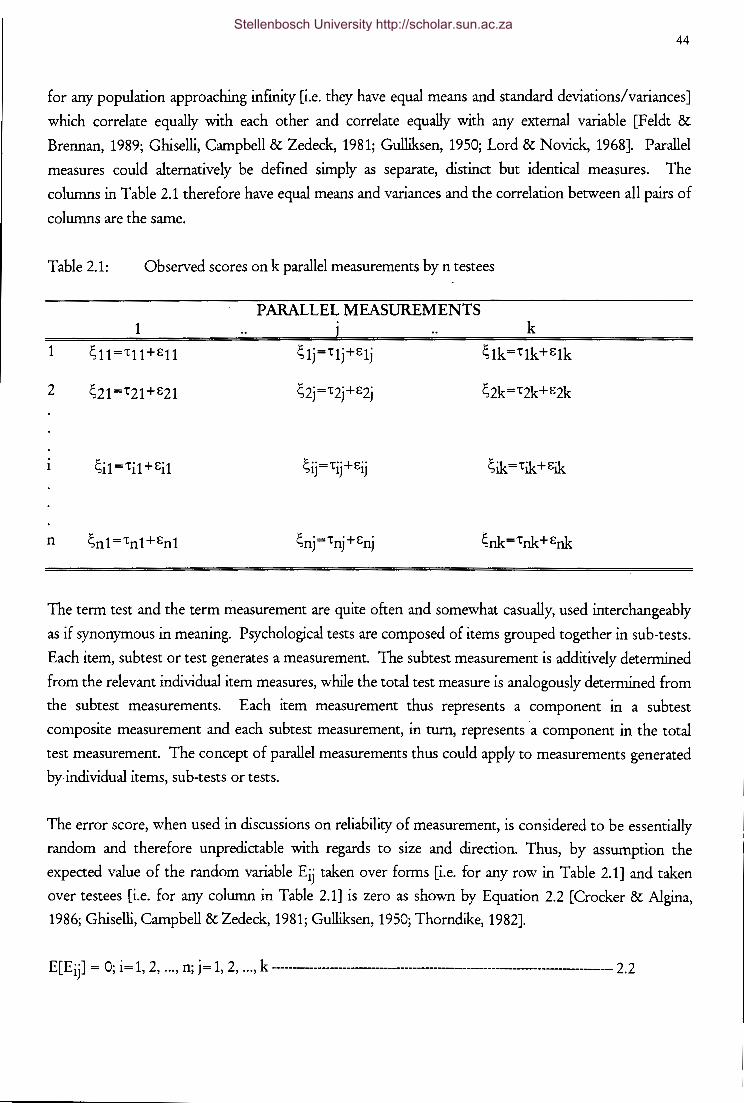
44
for any population approaching infinity [i.e. they have equal means and standard deviations/ variances]
which correlate equally with each other and correlate equally with any external variable [Feldt &
Brennan, 1989; Ghiselli, Campbell & Zedeck, 1981; Gulliksen, 1950; Lord & Novick, 1968]. Parallel
measures could alternatively be defined simply as separate, distinct but identical measures. The
columns in Table 2.1 therefore have equal means and variances and the correlation between all pairs of
columns are the same.
Table 2.1: Observed scores on k parallel measurements by n testees
1
2
n
1
~il ='til +Eil
~nt='tnt+Enl
PARALLEL MEASUREMENTS
~tj='ttj+Etj
~2j ='t2j + 82j
k
The term test and the term measurement are quite often and somewhat casually, used interchangeably
as if synonymous in meaning. Psychological tests are composed of items grouped together in sub-tests.
Each item, subtest or test generates a measurement. The subtest measurement is additively determined
from the relevant individual item measures, while the total test measure is analogously determined from
the subtest measurements. Each item measurement thus represents a component in a subtest
composite measurement and each subtest measurement, in turn, represents a component in the total
test measurement. The concept of parallel measurements thus could apply to measurements generated
by individual items, sub-tests or tests.
The error score, when used in discussions on reliability of measurement, is considered to be essentially
random and therefore unpredictable with regards to size and direction. Thus, by assumption the
expected value of the random variable Eij taken over forms [i.e. for any row in Table 2.1] and taken
over testees [i.e. for any column in Table 2.1] is zero as shown by Equation 2.2 [Crocker & Algina,
1986; Ghiselli, Campbell &Zedeck, 1981; Gulliksen, 1950; Thorndike, 1982].
. . k E[Eij] = 0; 1= 1, 2, ... , n; J= 1, 2, ... , ------------------------------------------------------------------------ 2.2
Stellenbosch University http://scholar.sun.ac.za
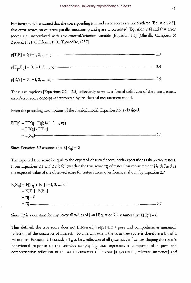
45
Furthermore it is assumed that the corresponding true and error scores are uncorrelated [Equation 2.3],
that error scores on different parallel measures p and q are uncorrelated [Equation 2.4] and that error
scores are uncorrelated with any external/ criterion variable [Equation 2.5] [Ghiselli, Campbell &
Zedeck, 1981; Gulliksen, 1950; Thorndike, 1982].
p[T,E] = 0; i= 1, 2, ... , n; j ------------------------------------------------------2.3
p[Ep,Eq] = 0; i= 1, 2, ... , n; j ----------------------------------------------- 2.4
p[E,Y] = 0; i= 1, 2, ... , n; j --------------------------------------------------------------2.5
These assumptions [Equations 2.2 - 2.5] collectively serve as a formal definition of the measurement
error I error score concept as interpreted by the classical measurement model.
From the preceding assumptions of the classical model, Equation 2.6 is obtained.
E[Tij] = E[Xij - Eij]; i= 1, 2, ... , n; j
= E[Xij] - E[Eij]
= E[Xij] --------------------------------------------------------------------------------------------- 2. 6
Since Equation 2.2 assumes that E[Eij] = 0
The expected true score is equal to the expected observed score; both expectations taken over testees.
From Equations 2.1 and 2.2 it follows that the true score 1"ij of testee i on measurement j is defined as
the expected value of the observed score for testee i taken over forms, as shown by Equation 2.7
E[Xij] = E[Tij + Eij]; j= 1, 2, ... , k; i
= E[Tij] - E[Eij]
= 1"ij- 0
- 1"" - lJ ------------------------------------------------------------------------------------------------- 2.7
Since Tij is a constant for any i over all values of j and Equation 2.2 assumes that E[Eij] = 0
Thus defined, the true score does not [necessarily] represent a pure and comprehensive numerical
reflection of the construct of interest. To a certain extent the term true score is therefore a bit of a
misnomer. Equation 2.1 considers Tij to be a reflection of all systematic influences shaping the testee's
behavioural response to the stimulus sample; Tij thus represents a composite of a pure and
comprehensive reflection of the stable construct of interest [a systematic, relevant influence] and
Stellenbosch University http://scholar.sun.ac.za
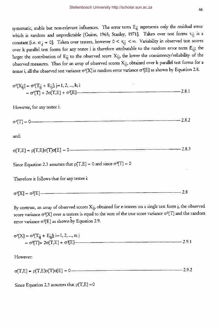
46
systematic, stable but non-relevant influences. The error term Eij represents only the residual error
which is random and unpredictable [Guion, 1965; Stanley, 1971]. Taken over test forms 'tij is a
constant [i.e. cr.j = 0]. Taken over testees, however 0 < 'tij < oo. Variability in observed test scores
over k parallel test forms for any testee i is therefore attributable to the random error term Eiji the
larger the contribution of Eij to the observed score Xij' the lower the consistency/reliability of the
observed measures. Thus for an array of observed scores Xij' obtained over k parallel test forms for a
testee i, all the observed test variance cr2[X] is random error variance cr2[E] as shown by Equation 2.8.
cr2[Xij] = cr2[Tij + Eij]; j= 1, 2, ... , k; i = cr2[T] + 2cr[T,E] + cr2[E]----------------------------------------------------- 2.8.1
However, for any testee i:
cr 2 [T] = 0----------------------------------------------------------------------------------------------------------- 2. 8. 2
and:
cr[T, E] = p[T ,E]cr[T]cr[E] = 0 -------------------------------------------------------------------------------------- 2. 8. 3
Since Equation 2.3 assumes that p[T,E] = 0 and since cr2[T] = 0
Therefore it follows that for any testee i:
cr 2 [X] = cr2[E] ------------------------------------------------------------------------------------------------------------ 2. 8
By contrast, an array of observed scores Xij' obtained for n testees on a single test form j, the observed
score variance cr2[X] over n testees is equal to the sum of the true score variance cr2[T] and the random •
error variance cr2[E] as shown by Equation 2.9.
cr2[X] = cr2[Tij + Eij]; i= 1, 2, ... , n; j
= cr2[T]+ 2cr[T,E] + cr2[E]-------------------------------------------------------- 2.9.1
However:
cr[T, E] = p[T, E] cr[T]cr[E] = 0 --------------------------------------------------------------------------------------- 2. 9. 2
Since Equation 2.3 assumes that p[T,E] =0
Stellenbosch University http://scholar.sun.ac.za
47
Therefore for any test form j:
cr2[XJ = cr2[1'] + cr2[E ]---------------------------------------------------------------------------------- 2. 9
If Equation 2.9 would subsequently be multiplied by 1/cr[X], Equation 2.10 results.
1 = cr2[1']/ cr2[XJ + cr2[E]/ cr2[X]---------------------------------------------------------- 2.10
2.5.1 Reliability
Reliability can be defined as consistency over parallel measures [Crocker & Algina, 1986]. Measures
tend to be consistent to the extent that they are free from variance due to random error influences.
Reliability can thus be defined as the extent to which a set of measures is free from random error
variance and consequently, given Equation 2.10, the ratio of true score variance to observed test score
variance. Nunnally [1978, p. 191] for example states:
Random errors of measurement are never completely eliminated; but to portray nature in its ultimate
lawfulness, efforts are made to reduce errors as much as possible. To the extent to which measurement error
is slight, a measure is set to be relidJ!e.
Guion [1965, p.30] in addition states:
Traditionally reliability has been defined as consistency of measurement. It has been virtually a synonym for
repeatability. Defined in this way, the concept is certainly useful, but not easily applied to day-to-day
measurement problems. The source of the consistency must be considered. . . . If the measures are
consistent they tend to be free from variance due to random errors. . .. As a basic concept, then reliability
can be defmed as the extent to ul?idJ a set of measures is frre from randon-envrwriance.
If a set of measures would be perfectly reliable, the observed test scores would be free of random
measurement error and consequently cr2[E] and thus cr2[E]/ cr2[X] would equal zero and cr2[TJ/ cr2[X]
would equal unity. Conversely, if a set of measures would be totally unreliable, the observed test score
would constitute nothing but random measurement error and consequently cr2[T] and thus cr2[TJ/ cr2[X]
would equal zero and cr2[E]/ cr2[X] would equal unity. Consequently, if the ratio of the true score
variance to the observed score variance [or conversely, the ratio of the error score variance to the
observed score variance] could be estimated, an appropriate indicator/measure of the reliability of a set
of score would be available. The quest for a quantitative measure of the reliability of a set of scores can
Stellenbosch University http://scholar.sun.ac.za
48
be approached from the two slightly dissimilar perspectives on inter-individual and intra-individual
variability [i.e. by either focussing on the columns or the rows in Table 2.1 ]. In terms of the inter
individual approach, an estimate of the extent to which the observed measures contain random
measurement error [i.e. are unreliable] is obtained through the consistency with which testees maintain
their rank-ordered position in the total group on parallel measures [Feldt & Brennan, 1989; Guion,
1965; Stanley, 1971]. In terms of the latter approach, however, an estimate of the extent to which the
observed measures contain random measurement error [i.e. are unreliable] is obtained through the
fluctuations in observed scores on parallel measures, expressed in score-scale units [Feldt & Brennan,
1989; Stanley, 1971].
Approaching the quest for a quantitative measure of the reliability of a set of scores from an inter
individual perspective on score variability, the covariance and correlation between observed scores and
true scores are subsequently examined.
cr[Xij,Tij] = E[XijTij] - E[Xij]E[Tij]; i= 1, 2, ... , n; j
= E[(fij+ Eij)Tij]- E[(fij + Eij)]E[Tij]
- E[T2··] + E[E··T·]- E[T-·]2 -E[E··]E[T··] - lJ lJ lJ lJ lJ lJ = cr2[T] + E[EijTij]- E[Eij]E[Tij}--------------------------------------------------------------- 2.11.1
However, according to Equation 2.2, E[Eij] = 0 and, cr[T,E] = p[T,E]cr[T]cr[E] = 0
Since, according to Equation 2.3, p[T,E] =0.
Hence:
cr[Xij,Tij] = cr[X,T] = cr2[T]-------------------------------------------------------------------------------- 2.11.2
However, by definition:
p2[X, T] = cr2[X, T]/ ( cr2[X]cr2[T]) ----------------------------------------------------------------- 2.11. 3
Thus, by substituting in accordance with Equation 2.11.2, Equation 2.11.3 becomes:
p2[X,T] = cr4[T]/ ( cr2[X]cr2[T])
= cr2[T]/ cr2[X]-------------------------------------------------------------------------------------- 2.11
The square of the correlation between observed scores and true scores equals the ratio of the true score
variance to the observed score variance. The quantity, p[X,T] = cr[T]/cr[X], is referred to as the index
of reliability [Guion, 1965; Gulliksen, 1950; Lord & Novick, 1968]. From an inter-individual variability
Stellenbosch University http://scholar.sun.ac.za
49
perspective, the square of the index of reliability [i.e. interpreted in terms of the coefficient of
determination] thus provides a quantitative description of the reliability of a set of scores. From
Equation 2.9 and Equation 2.11, Equation 2.12 is obtained.
According to Equation 2.11,
p2[X,T] = cr2[T]/ cr2[X]
= 1- (cr2[E]/cr2[X])--------------------------------------------- 2.12
Since according to Equation 2.9, cr2[X] = cr2[T] + cr2[E]
Thus the square of the correlation between the observed scores and true scores could also be
interpreted as the proportion of observed test variance remaining once the random error variance has
been removed. Using a procedure similar to that followed to obtain Equation 2.11, it could be shown
[Equation 2.13] that the square of the correlation between the observed scores and error scores equals
the ratio of random error variance to observed score variance.
crCXij,Eij] = ECXijEij] - E[Xij]E[Eij]; i= 1, 2, ... , n; j
= E[Cfij+ Eij)Eij]- E[Cfij + Eij)]E[Eij]
- E[E2··] + E[E··T·] E[E··]2 E[E··]E[T··] - lJ lJ lJ - lJ - lJ lJ = cr2E + E[EijTij] - E[Eij]E[TijJ-------------------------------------------------------------------- 2.13.1
However according to Equation 2.2, E[Eij] = 0 and, cr[T,E] = p[T,E]cr[T]cr[E] = 0
Since according to Equation 2.3, p[T,E] =0.
Hence:
crCXij ,Ei j] = cr[X,E] = cr2[E }--------------------------------------------------------------------- 2.13. 2
However, by definition:
p2[X, E] = crz[X,E ]I ( cr2[X]cr2[E ]) ----------------------------------------------------------------- 2.13. 3
Thus, by substituting in accordance with Equation 2.13.2, Equation 2.13.3 becomes:
p2[X,E] = cr4[E]/ ( cr2[X]cr2[E])
= cr2[E ]/ cr2[X]------------------------------------------------------------------------------------------ 2.13
Stellenbosch University http://scholar.sun.ac.za
50
Although interlocking perfectly with the conceptual definition of reliability, neither the index of
reliability [Equation 2.11], nor Equation 2.13, could, however, be computed directly. A practical
measure/indicator of the reliability of a set of observed measures can, however, be obtained by
expressing the unobservable index of reliability in terms of a parameter of the bivariate observed score
distribution.
2.5.1.1 Reliability Estimates
Assume two classically parallel measures p and q. From the definition of parallel measures follows that
J.lp = E[Tip] = J.lq = E[TiqJ. According to Equation 2.14 the correlation between two truly parallel
measures, applied such that Tip = Tiq over all values of i [i.e. no practice, fatigue, memoty or any other
systematic method factor affects the repeated measurement], equals the ratio of the true score variance
to the observed score variance.
From the basic definition formula, it follows that:
p[Xip,Xiq] = cr[Xip,XiqJ/ ( cr[Xip]cr[Xiq]; i = 1, 2, ... n; j = p, q---------------------------------------- 2.14 .1
However:
cr[Xip,Xiq] = E[XipXiq] - E[Xip]E[Xiq]
= E[(Tip+Eip)(Tiq+Eiq)J- E[(Tip+Eip)]E[(Tiq+Eiq)J
= E[(Ti+Eip)(Ti +Eiq)J- E[(Ti +Eip)]E[(Ti + Eiq)J--------------------------------2.14.2
Since from the tenants of the classical measurement model it follows that:
Tip = Tiq; i= 1, 2, ... n; j=p, q
Thus:
cr[Xip,Xiq] = E[TiTi]+ 2E[EijTi]+ E[EipEiqHE[Ti] + E[EipJIE[Ti] + E[Eiq]]
= E[T?J+2E[EijTi]+E[EipEiqJ-E[Ti]E[Ti]+E[EipJE[Ti]+E[Ti]E[Eiq]+
E[Eiq]E[Ei p] ------------------------------------------------------------------------~----- 2.14. 3
However according to Equation 2.2, E[EipJ = E[Eiq] = 0
Stellenbosch University http://scholar.sun.ac.za
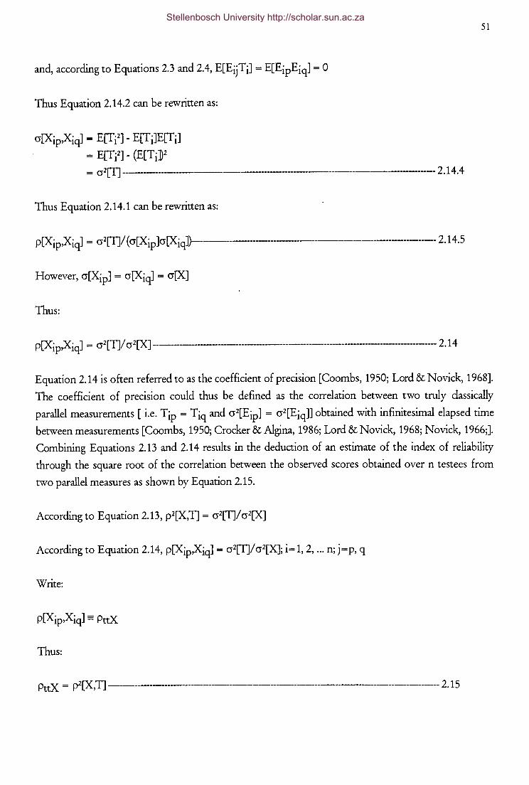
and, according to Equations 2.3 and 2.4, E[EijTi] = E[EipEiqJ = 0
Thus Equation 2.14.2 can be rewritten as:
cr[Xip,Xiq] = E[T?J- E[Ti]E[Ti]
= E[Ti2]- (E[Ti]z
= cr2[T] -------------------------------------------------------------------- 2.14. 4
Thus Equation 2.14.1 can be rewritten as:
p[XipXiqJ = cr2[T]I ( cr[Xip]cr[Xiq]}-------------------------------------------------------- 2.14 .5
However, cr[XipJ = cr[XiqJ = cr[X]
Thus:
p[Xip,Xiq] = cr2[T]/ cr2[X] ----------------------------------------------------------------------------------- 2.14
51
Equation 2.14 is often referred to as the coefficient of precision [Coombs, 1950; Lord & Novick, 1968].
The coefficient of precision could thus be defined as the correlation between two truly classically
parallel measurements [i.e. Tip = Tiq and cr2[EipJ = cr2[EiqJJ obtained with infinitesimal elapsed time
between measurements [Coombs, 1950; Crocker & Algina, 1986; Lord & Novick, 1968; Novick, 1966;].
Combining Equations 2.13 and 2.14 results in the deduction of an estimate of the index of reliability
through the square root of the correlation between the observed scores obtained over n testees from
two parallel measures as shown by Equation 2.15.
According to Equation 2.13, p2[X,T] = cr2[T]/ cr2[X]
According to Equation 2.14, p[XipXiq] = cr2[T]Icr2[X]; i= 1, 2, ... n; j=p, q
Write:
Thus:
PttX = pz[X, T] ----------------------------------------------------------------------------------------------------- 2.15
Stellenbosch University http://scholar.sun.ac.za

52
Contingent on the assumption that at least one pair of classically parallel measures are available,
Equation 2.15 equates the conceptually pleasing, but empirically unobservable, quantity p2[X, T] to the
observable quality PitX [Lord & Novick, 1968].
Rearranging the terms in Equation 2.15 through cross multiplication, Equation 2.16 is obtained.
Write p[Xip,XiqJ = PttXi i=1, 2, ... n; j=p, q
Thus, according to Equation 2.14, PttX = cr2[TJ/ cr2[X]
Thus:
cr2[TJ = PttXcr2[XJ ------------------------------------------------------------------------------------ 2.16
According to Equation 2.16 the true score variance is equal to, and thus can be estimated by, the
product of the observed score variance and the correlation between parallel measurements. The error
score variance, in contrast, is equal to the product of the observed score variance and one minus the
correlation between parallel measurements, as shown by Equation 2.17.
According to Equation 2.16, cr2[T] = PttXcr2[X]
According to Equation 2.9, cr2[X] = cr2[T] + cr2[E]
Thus, by substituting Equation 2.16 into Equation 2.9 it follows that::
cr2[X] = PttXcr2[X] + cr2[E] -------------------------------------------------------------------------------- 2.17 .1
Thus cr2[E] = cr2[X] - PttXcr2[X]
= cr2[X][ 1 -PttXJ--------------------------------------------------------------------------------- 2.17
By taking square roots, Equation 2.17 can be written as Equation 2.18, which defines the standard error
of measurement.
According to Equation 2.17, cr2[E] = cr2[X] - PttXcr2[X]
By taking square roots it thus follows that::
cr[ E] = cr[X]~[ 1 - PttXJ ---------------------------------------------------------------------------------------------- 2.18
Stellenbosch University http://scholar.sun.ac.za
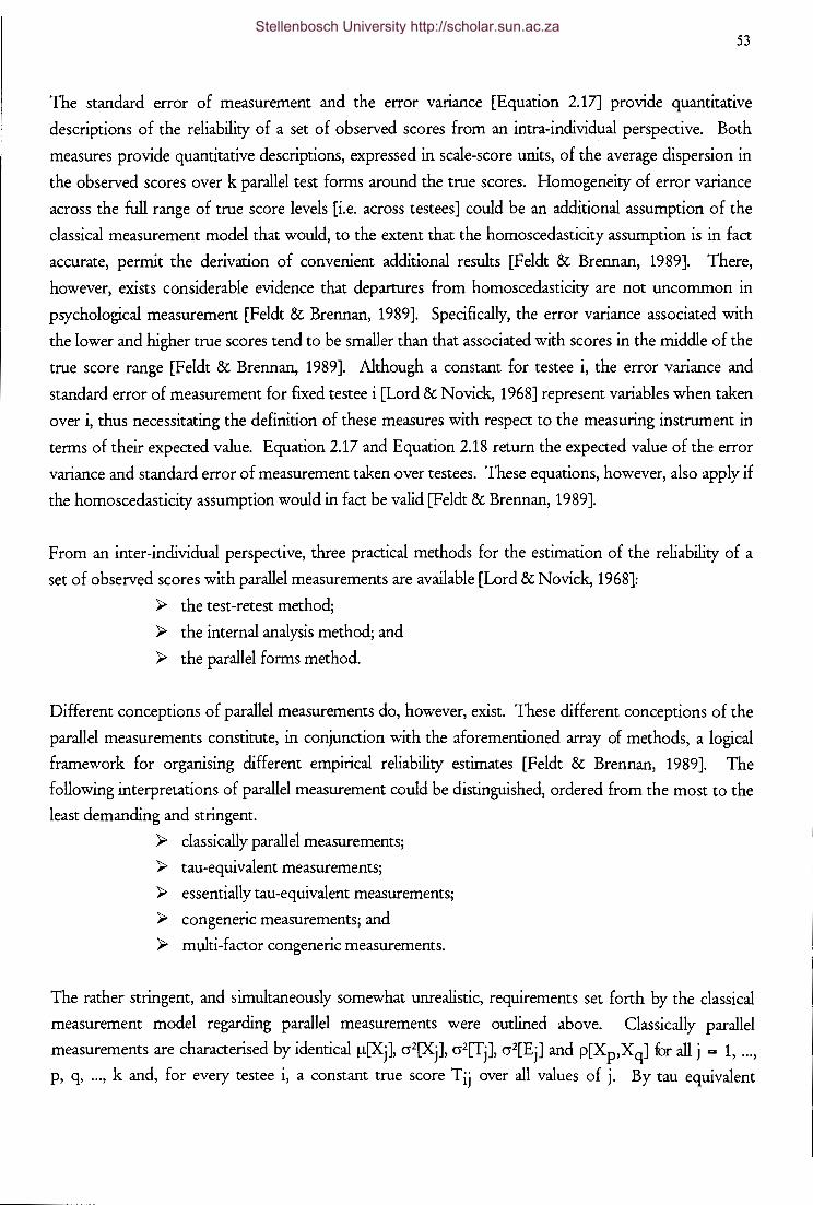
53
The standard error of measurement and the error vanance [Equation 2.17] provide quantitative
descriptions of the reliability of a set of observed scores from an intra-individual perspective. Both
measures provide quantitative descriptions, expressed in scale-score units, of the average dispersion in
the observed scores over k parallel test forms around the true scores. Homogeneity of error variance
across the full range of true score levels [i.e. across testees] could be an additional assumption of the
classical measurement model that would, to the extent that the homoscedasticity assumption is in fact
accurate, permit the derivation of convenient additional results [Feldt & Brennan, 1989]. There,
however, exists considerable evidence that departures from homoscedasticity are not uncommon in
psychological measurement [Feldt & Brennan, 1989]. Specifically, the error variance associated with
the lower and higher true scores tend to be smaller than that associated with scores in the middle of the
true score range [Feldt & Brennan, 1989]. Although a constant for testee i, the error variance and
standard error of measurement for fixed testee i [Lord & Novick, 1968] represent variables when taken
over i, thus necessitating the definition of these measures with respect to the measuring instrument in
terms of their expected value. Equation 2.17 and Equation 2.18 return the expected value of the error
variance and standard error of measurement taken over testees. These equations, however, also apply if
the homoscedasticity assumption would in fact be valid [Feldt & Brennan, 1989].
From an inter-individual perspective, three practical methods for the estimation of the reliability of a
set of observed scores with parallel measurements are available [Lord & Novick, 1968]:
);> the test-retest method;
);> the internal analysis method; and
);> the parallel forms method.
Different conceptions of parallel measurements do, however, exist. These different conceptions of the
parallel measurements constitute, in conjunction with the aforementioned array of methods, a logical
framework for organising different empirical reliability estimates [Feldt & Brennan, 1989]. The
following interpretations of parallel measurement could be distinguished, ordered from the most to the
least demanding and stringent.
);> classically parallel measurements;
);> tau-equivalent measurements;
);> essentially tau-equivalent measurements;
);> congeneric measurements; and
);> multi-factor congeneric measurements.
The rather stringent, and simultaneously somewhat unrealistic, requirements set forth by the classical
measurement model regarding parallel measurements were outlined above. Classically parallel
measurements are characterised by identical !J.[Xj], cr2[Xj], cr2[Tj], cr2[Ej] and p[Xp,Xq] br all j = 1, ... ,
p, q, ... , k and, for every testee i, a constant true score Tij over all values of j. By tau equivalent
Stellenbosch University http://scholar.sun.ac.za
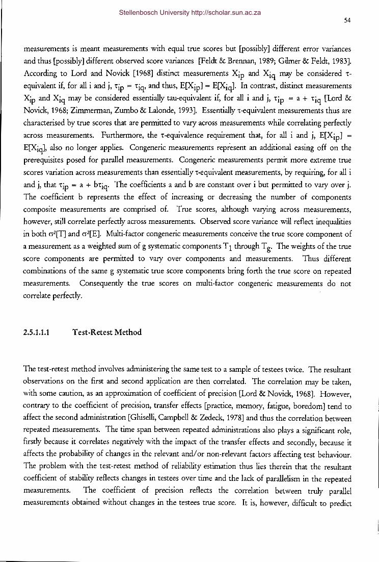
54
measurements is meant measurements with equal true scores but [possibly] different error variances
and thus [possibly] different observed score variances [Feldt & Brennan, 1989; Gilmer & Feldt, 1983].
According to Lord and Novick [1968] distinct measurements Xip and Xiq may be considered '!
equivalent if, for all i and j, 'tip = 'tiq• and thus, E[XipJ = E[XiqJ· In contrast, distinct measurements
Xip and Xiq may be considered essentially tau-equivalent if, for all i and j, 'tip = a + 'tiq [Lord &
Novick, 1968; Zimmerman, Zumbo & Lalonde, 1993]. Essentially '!-equivalent measurements thus are
characterised by true scores that are permitted to vary across measurements while correlating perfectly
across measurements. Furthermore, the '!-equivalence requirement that, for all i and j, E[XipJ =
E[Xiq], also no longer applies. Congeneric measurements represent an additional easing off on the
prerequisites posed for parallel measurements. Congeneric measurements permit more extreme true
scores variation across measurements than essentially '!-equivalent measurements, by requiring, for all i
and j, that 'tip = a + b'tiq· The coefficients a and b are constant over i but permitted to vary over j. The coefficient b represents the effect of increasing or decreasing the number of components
composite measurements are comprised of. True scores, although varying across measurements,
however, still correlate perfectly across measurements. Observed score variance will reflect inequalities
in both cr2[T] and cr2[E]. Multi-factor congeneric measurements conceive the true score component of
a measurement as a weighted sum of g systematic components T 1 through T g· The weights of the true
score components are permitted to vary over components and measurements. Thus different
combinations of the same g systematic true score components bring forth the true score on repeated
measurements. Consequently the true scores on multi-factor congeneric measurements do not
correlate perfectly.
2.5.1.1.1 Test-Retest Method
The test-retest method involves administering the same test to a sample of testees twice. The resultant
observations on the first and second application are then correlated. The correlation may be taken,
with some caution, as an approximation of coefficient of precision [Lord & Novick, 1968]. However,
contrary to the coefficient of precision, transfer effects [practice, memory, fatigue, boredom J tend to
affect the second administration [Ghiselli, Campbell & Zedeck, 1978] and thus the correlation between
repeated measurements. The time span between repeated administrations also plays a significant role,
firstly because it correlates negatively with the impact of the transfer effects and secondly, because it
affects the probability of changes in the relevant and/ or non-relevant factors affecting test behaviour.
The problem with the test-retest method of reliability estimation thus lies therein that the resultant
coefficient of stability reflects changes in testees over time and the lack of parallelism in the repeated
measurements. The coefficient of precision reflects the correlation between truly parallel
measurements obtained without changes in the testees true score. It is, however, difficult to predict
Stellenbosch University http://scholar.sun.ac.za
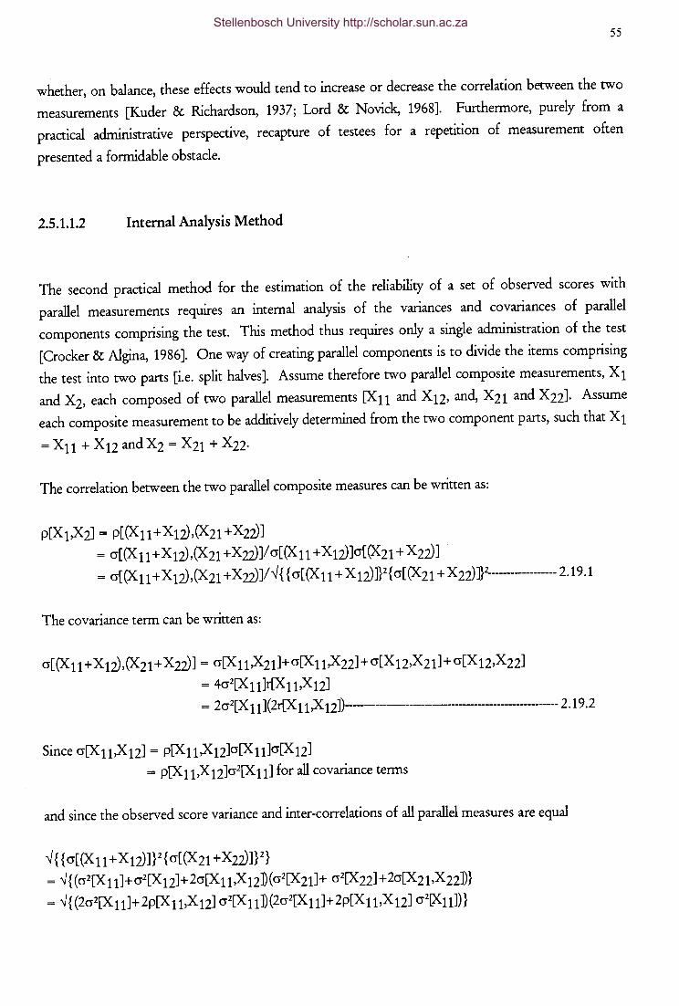
55
whether, on balance, these effects would tend to increase or decrease the correlation between the two
measurements [Kuder & Richardson, 1937; Lord & Novick, 1968]. Furthermore, purely from a
practical administrative perspective, recapture of testees for a repetition of measurement often
presented a formidable obstacle.
2.5.1.1.2 Internal Analysis Method
The second practical method for the estimation of the reliability of a set of observed scores with
parallel measurements requires an internal analysis of the variances and covariances of parallel
components comprising the test. This method thus requires only a single administration of the test
[Crocker & Algina, 1986]. One way of creating parallel components is to divide the items comprising
the test into two parts [i.e. split halves]. Assume therefore two parallel composite measurements, X 1
and X2, each composed of two parallel measurements [X11 and X12, and, X21 and X22J· Assume
each composite measurement to be additively determined from the two component parts, such that X 1
= x11 + x12 and x2 = X21 + X22·
The correlation between the two parallel composite measures can be written as:
p[X1,X2J = p[(X11+X12),(X21 +X22)J
= cr[(X11+X12),(X21 +X22)]/cr[(X11 +X12)]cr[(X21 +X22)J
= cr[(X 11 +X 12),(X21 +X22)J/"{ { cr[(X 11 +X 12)]}2{ cr[(X21 + X22)]}2------------------- 2.19.1
The covariance term can be written as:
cr[(X11 +X12),(X21 +X22)J = cr[X11,X21]+cr[X11,X22]+cr[X12,X21]+cr[X12,X22]
= 4cr2[X 11Jr[X 11,X 12J
= 2cr2[X 11](2r[X 11 ,X 12])---------------------------------- 2.19 .2
Since cr[X 11,X 12J = p[X 11,X 12Jcr[X 11Jcr[X 12J
= p[X 11 ,X 12]cr2[X 11J for all covariance terms
and since the observed score variance and inter-correlations of all parallel measures are equal
"{ { cr[(X 11 +X 12)]}2{ cr[(X21 +X22)]}2}
= "{ (cr2[X 11J+cr2[X 12]+2cr[X 11,X 12Ncr2[X21J+ cr2[X22J +2cr[X21,X22J)}
= "{ (2cr2[X 11]+2p[X 11,X 12J cr2[X 11])(2cr2[X 11]+2p[X 11,X 12J cr21X11J)}
Stellenbosch University http://scholar.sun.ac.za
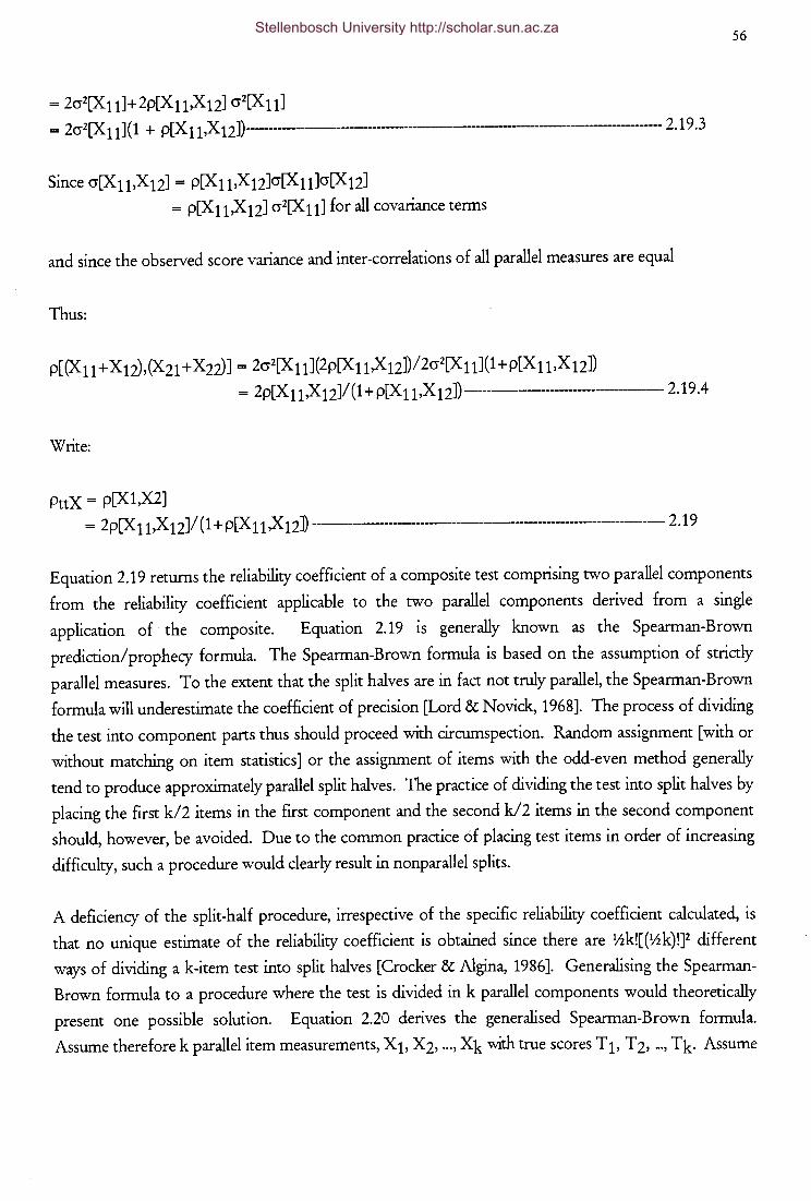
56
= 2cr2[X11]+2p[X11,X12] cr2[X11]
= 2cr2[X 11](1 + p[X 11,X 12])---------------------------------------- 2.19 .3
Since cr[X 11 ,X 12J = p[X 11 ,X 12Jcr[X 11Jcr[X 12J
= p[X 11X 12J cr2[X 11J for all covariance terms
and since the observed score variance and inter-correlations of all parallel measures are equal
Thus:
p[(X 11 +X12),(X21 +X22)J = 2cr2[X 11](2p[X 11X 12])/2cr2[X 11](1 +p[X 11,X 12])
= 2p[X 11,x 12J/ (1 + p[X 11,x 12J) --------------------------- 2.19 .4
Write:
PttX = p[X1,X2] = 2p[X 11,x 12J/ ( 1 + p[X 11 ,x 12J) ------------------------------------------------------------------- 2.19
Equation 2.19 returns the reliability coefficient of a composite test comprising two parallel components
from the reliability coefficient applicable to the two parallel components derived from a single
application of the composite. Equation 2.19 is generally known as the Spearman-Brown
prediction/prophecy formula. The Spearman-Brown formula is based on the assumption of strictly
parallel measures. To the extent that the split halves are in fact not truly parallel, the Spearman-Brown
formula will underestimate the coefficient of precision [Lord & Novick, 1968]. The process of dividing
the test into component parts thus should proceed with circumspection. Random assignment [with or
without matching on item statistics] or the assignment of items with the odd-even method generally
tend to produce approximately parallel split halves. The practice of dividing the test into split halves by
placing the first k/2 items in the first component and the second k/2 items in the second component
should, however, be avoided. Due to the common practice of placing test items in order of increasing
difficulty, such a procedure would clearly result in nonparallel splits.
A deficiency of the split-half procedure, irrespective of the specific reliability coefficient calculated, is
that no unique estimate of the reliability coefficient is obtained since there are lhk![(t,~k)!]2 different
ways of dividing a k-item test into split halves [Crocker & Algina, 1986]. Generalising the Spearman
Brown formula to a procedure where the test is divided in k parallel components would theoretically
present one possible solution. Equation 2.20 derives the generalised Spearman-Brown formula.
Assume therefore k parallel item measurements, X 1, X2, ... , Xk with true scores T 1, T 2, -·, Tk. Assume
Stellenbosch University http://scholar.sun.ac.za
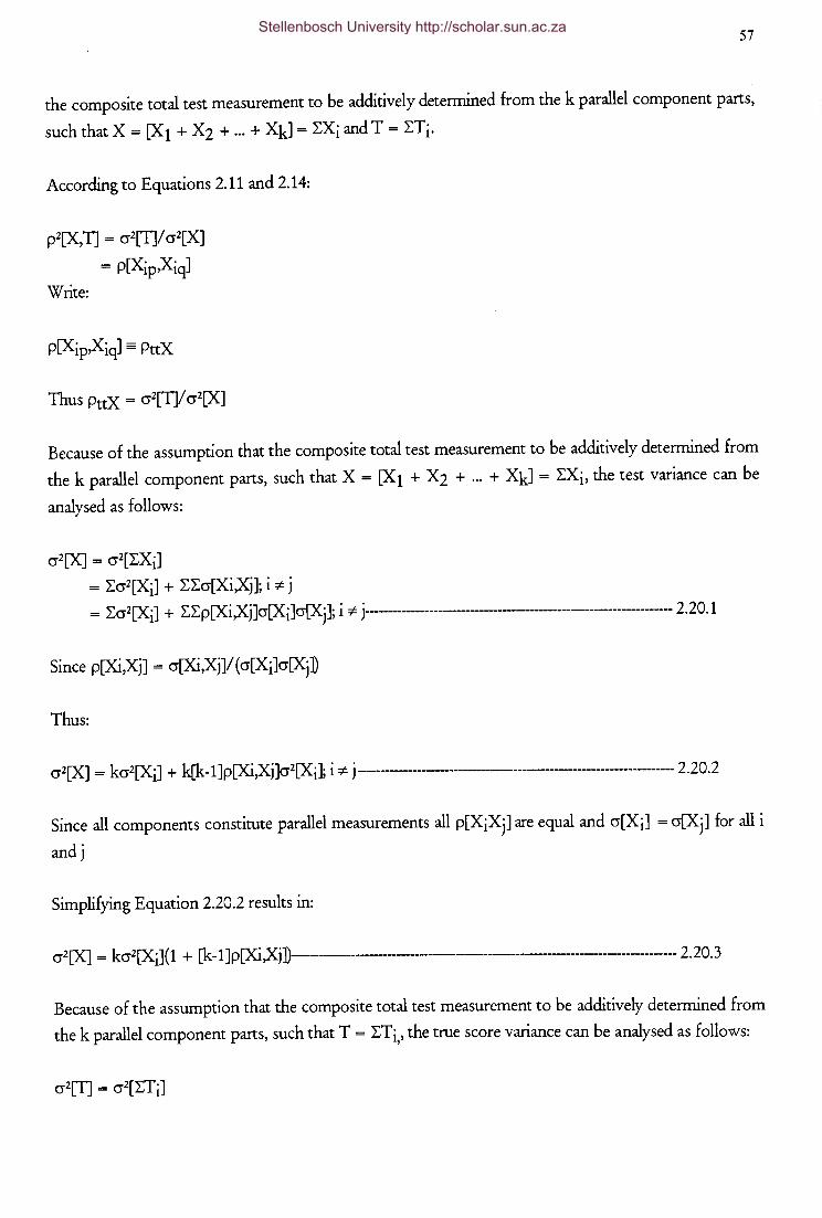
57
the composite total test measurement to be additively determined from the k parallel component parts,
such that X= [X1 + X2 + ... + Xk] = LXi and T = LTi.
According to Equations 2.11 and 2.14:
p2[X,T] = cr2[T]/ cr2[X]
= p[Xip,Xiq]
Write:
Because of the assumption that the composite total test measurement to be additively determined from
the k parallel component parts, such that X = [X 1 + X2 + ... + Xk] = LXi, the test variance can be
analysed as follows:
cr2[X] = cr2[LXi]
= Lcr2[Xi] + LLcr[Xi,Xj]; i -:t j
= Lcr2[Xi] + LLp[Xi,Xj]cr[Xi]cr[Xj]; i -:t j------------------------------------------------------------ 2.20.1
Since p[Xi,Xj] = cr[Xi,Xj]/ ( cr[Xi]cr[Xj]
Thus:
cr2[X] = kcr2[Xi] + k[k-1]p[Xi,Xj]cr2[Xi]; i -:t j------------------------------------------------ 2.20.2
Since all components constitute parallel measurements all p[XiXj] are equal and cr[Xi] = cr[Xj] for all i
andj
Simplifying Equation 2.20.2 results in:
cr2[X] = kcr2[Xi] ( 1 + [k -1] p[Xi,Xj])---------------------------------------------------------------- 2.20. 3
Because of the assumption that the composite total test measurement to be additively determined from
the k parallel component parts, such that T = LTi,, the true score variance can be analysed as follows:
Stellenbosch University http://scholar.sun.ac.za
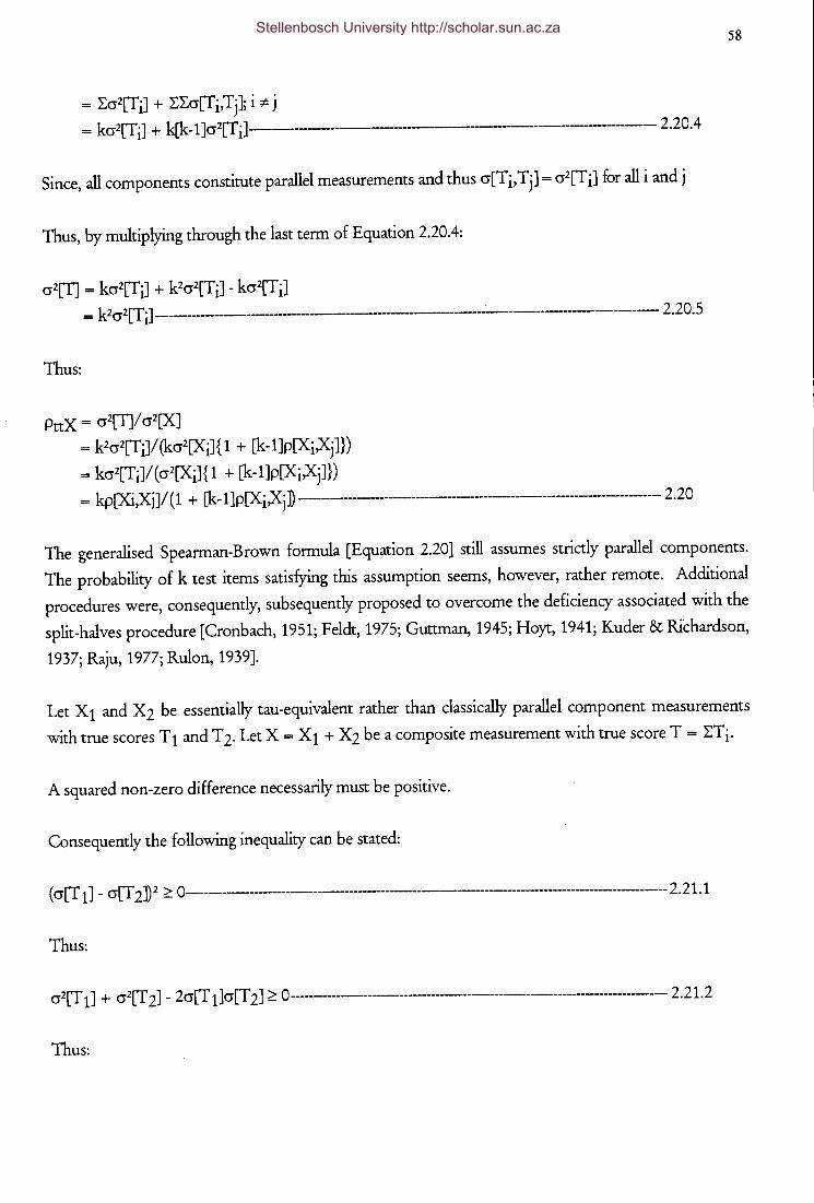
= :Ecr2[Ti] + :E:Ecr[Ti,Tj]; i * j = kcr2[Ti] + k[k-1]cr2[TiJ------------------------------------------------ 2.20.4
Since, all components constitute parallel measurements and thus cr[Ti,Tj] = cr2[Ti] for all i and j
Thus, by multiplying through the last term of Equation 2.20.4:
cr2[T] = kcr2[Ti] + k2cr2[Ti]- kcr2[Ti] = k2cr2[Ti] ___________________________________________ _: ________________________ 2.20.5
Thus:
PttX = cr2[T]/ cr2[X]
= k2cr2[Ti]/ (kcr2[Xi]{ 1 + [k-1 ]p[XiXj]})
= kcr2[Ti]/(cr2[Xi]{1 + [k-1]p[XiXj]})
= kp[Xi,Xj]/ ( 1 + [k-1 ]p[XiXj] ---------------------------------------------------------------- 2.20
58
The generalised Spearman-Brown formula [Equation 2.20] still assumes strictly parallel components.
The probability of k test items satisfying this assumption seems, however, rather remote. Additional
procedures were, consequently, subsequently proposed to overcome the deficiency associated with the
split-halves procedure [Cronbach, 1951; Feldt, 1975; Guttman, 1945; Hoyt, 1941; Kuder & Richardson,
1937; Raju, 1977; Rulon, 1939].
Let X 1 and X2 be essentially tau-equivalent rather than classically parallel component measurements
with true scores T 1 and T 2. Let X = X 1 + X 2 be a composite measurement with true score T = :ETi.
A squared non-zero difference necessarily must be positive.
Consequently the following inequality can be stated:
( cr[T 1J - cr[T 2])2 ~ 0----------------------------------------------------------------------- 2.21.1
Thus:
cr2[T 1J + cr2[T 2J- 2cr[T 1Jcr[T 2J ~ 0--------------------------------------------------------------------------2.21.2
Thus:
Stellenbosch University http://scholar.sun.ac.za
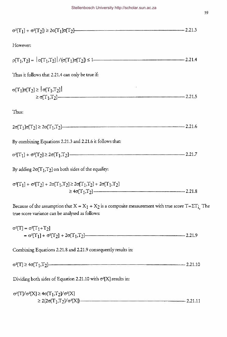
----------------------------------.
59
cr2[T 1] + cr2[T 2]) ~ 2cr[T 1]cr[T 2}---------------------------------------------------------- 2.21.3
However:
p[T1,T2] = I cr[T1,T2J I /(cr[T1]cr[T2] ~ 1-----------------------------------------------2.21.4
Thus it follows that 2.21.4 can only be true if:
cr[T 1Jcr[T 2J ~ I cr[T 1,T 2J I ~ cr[T 1, T 2] ----------------------------------------------------------------------- 2.21. 5
Thus:
2cr[T 1Jcr[T 2J ~ 2cr[T 1, T 2]---------------------------------------------------------------------------------------- 2.21. 6
By combining Equations 2.21.3 and 2.21.6 it follows that:
cr2[T 1] + cr2[T 2] ~ 2cr[T 1, T 2] -------------------------------------------------------------------------------- 2. 21.7
By adding 2cr[T 1,T 2] on both sides of the equality:
cr2[T1] + cr2[T2] + 2cr[T1,T2J~ 2cr[T1,T2J + 2cr[T1,T2]
~ 4cr[T 1, T 2] -------------------------------------------------------------- 2. 21. 8
Because of the assumption that X = X 1 + X2 is a composite measurement with true score T =L:Ti The , true score variance can be analysed as follows:
cr2[T] = cr2[T 1 + T 2]
= cr2[T 1J + cr2[T 2] + 2cr[T 1,T 2]--------------------------------------------------------------- 2.21.9
Combining Equations 2.21.8 and 2.21.9 consequently results in:
cr2[T] ~ 4cr[T 1, T 2}------------------------------------------------------------------------------------ 2. 21.10
Dividing both sides of Equation 2.21.10 with cr2[X] results in:
cr2[T]/ cr2[X] ~ 4cr[T 1,T 2]/ cr2[X]
~ 2 ( 2cr[T 1, T 2]/ cr2[X]) ----------------------------------------------------------------------------- 2.21.11
Stellenbosch University http://scholar.sun.ac.za
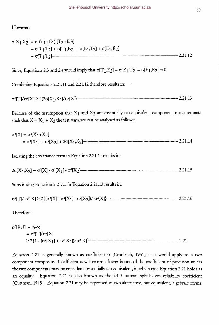
60
However:
cr[X1X2J = cr[(f1+E1),(T2+E2)]
= cr[T1,T2] + cr[f1,E2] + cr[E1,T2] + cr[E1,E2]
= cr[f hT 2J ------------------------------------------- 2.21.12
Since, Equations 2.3 and 2.4 would imply that cr[f 1 ,E 2J = cr[E 1, T 2J = cr[E 1 ,E 2J = 0
Combining Equations 2.21.11 and 2.21.12 therefore results in:
cr2[TJ/ cr2[XJ ;::: 2 ( 2cr[X 1 ,X 2J/ cr2[X])--------------------------------------------------------------- 2.21.13
Because of the assumption that X 1 and X2 are essentially tau-equivalent component measurements
such that X = X 1 + X2 the test variance can be analysed as follows:
cr2[X] = cr2[X 1 + X2J
= cr2[X 1J + cr2[X 2J + 2cr[X 1 ,X 2}-------------------------------------------------------------- 2.21.14
Isolating the covariance term in Equation 2.21.14 results in:
2cr[X 1 ,X 2J = cr2[X] - cr2[X 1J - cr2[X 2]------------------------------------------------------------------------ 2.21.15
Substituting Equation 2.21.15 in Equation 2.21.13 results in:
cr2[f]/ cr2[XJ;::: 2{(cr2[X]- cr2[X1J- cr2[X2])/ cr2[X]}------------------------------------------------2.21.16
Therefore:
P2[X,T] = PttX
= cr2[TJ/ cr2[XJ
2:: 2 { 1 - ( cr2[X 1J + cr2[X 2J) I cr2[XJ} --------------------------------------------------- 2.21
Equation 2.21 is generally known as coefficient a [Cronbach, 1951] as it would apply to a two
component composite. Coefficient a will return a lower bound of the coefficient of precision unless
the two components may be considered essentially tau-equivalent, in which case Equation 2.21 holds as
an equality. Equation 2.21 is also known as the AA Guttman split-halves reliability coefficient
[Guttman, 1945]. Equation 2.21 may be expressed in two alternative, but equivalent, algebraic forms.
Stellenbosch University http://scholar.sun.ac.za
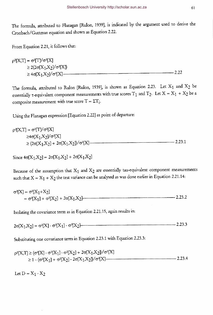
61
The formula, attributed to Flanagan [Rulon, 1939], is indicated by the argument used to derive the
CronbachiGuttman equation and shown as Equation 2.22.
From Equation 2.21, it follows that:
p2[X,T] = az[T]I cr2[X]
~ 2(2cr[X 1,X2]I cr2[X] ~ 4cr[X 1X2JI cr2[X] ------------------------------------------------ 2.22
The formula, attributed to Rulon [Rulon, 1939], is shown as Equation 2.23. Let X1 and X2 be
essentially '!-equivalent component measurements with true scores T 1 and T 2· Let X = X 1 + X2 be a
composite measurement with true score T = L:Ti.
Using the Flanagan expression [Equation 2.22] as point of departure:
p2[X,T] = cr2[T]I cr2[X]
~4cr[X 1X2JI cr2[X] ~ ( 2cr[X 1 ,X 2J + 2cr[X 1 ,X 2J) I cr2[X] --------------------------------------------------------------------- 2.23 .1
Because of the assumption that X 1 and X2 are essentially tau-equivalent component measurements
such that X= X 1 + X2 the test variance can be analysed as was done earlier in Equation 2.21.14:
cr2[XJ = cr2[X 1 +X 2] = cr2[X 1J + cr2[X2] + 2cr[X 1X2}-------------------------------------------------------------------- 2.23.2
Isolating the covariance term as in Equation 2.21.15, again results in:
2cr[X 1X2J = cr2[X] - cr2[X 1J - cr2[X2]-------------------------------------------------------------------- 2.23.3
Substituting one covariance term in Equation 2.23.1 with Equation 2.23.3:
p2[X,T] ~ (cr2[XJ- cr2[X1]- cr2[X2] + 2cr[X1,X2J)Icr2[X] ~ 1 - ( cr2[X 1J + cr2[X 2J - 2cr[X 1 ,X 2] I cr2[X] ------------------------------------------------------ 2.23. 4
Stellenbosch University http://scholar.sun.ac.za
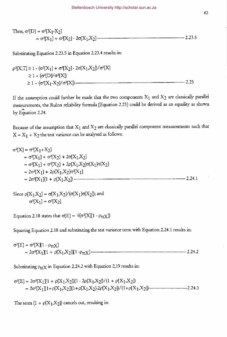
Then, cr2[D] = cr2[X 1-X 2J = cr2[X 1J + cr2[X 2J - 2cr[X 1 ,X 2J ---------------------------------------- 2.23 .5
Substituting Equation 2.23.5 in Equation 2.23.4 results in:
p2[X,T] ~ 1- (cr2[X1J + cr2[X2]- 2cr[Xl,X2])/cr2[X]
~ 1- (cr2[D]/cr2[XJ) ~ 1 - ( cr2[X 1-X 2J/ cr2[X])--------------------------------------------------- 2.23
62
If the assumption could further be made that the two components X 1 and X 2 are classically parallel
measurements, the Rulon reliability formula [Equation 2.23] could be derived as an equality as shown .....
by Equation 2.24.
Because of the assumption that X 1 and X2 are classically parallel component measurements such that
X = X 1 + X2 the test variance can be analysed as follows:
cr2[XJ = cr2[X 1 + X2]
= cr2[X 1J + cr2[X2] + 2cr[X 1X2J
= cr2[X 1J + cr2[X2] + 2p[X 1X2Jcr[X 1Jcr[X2J
= 2cr2[X 1J + 2p[X 1,X 2Jcr2[X 1J
= 2cr2[X 1J ( 1 + p[X 1 ,X 2] ----------------------------------------------------------------------------------- 2. 2 4.1
Since p[X1,X2J = cr[X1,X2]/(cr[X1]cr[X2]); and
cr2[X 1] = cr2[X2]
Equation 2.18 states that cr[E] = --J(cr2[X][l - PttX])
Squaring Equation 2.18 and substituting the test variance term with Equation 2.24.1 results in:
cr2[E] = cr2[X][l - PttXJ = 2cr2[X til + p[X 1X2]][l -PttX] ----------------------------------------------------------------- 2.24.2
Substituting PttX in Equation 2.24.2 with Equation 2,19 results in:
cr2[E] = 2cr2[Xt][l + p[X1X2JJ(l- 2p[X1X2]/(1 + p[Xt,X2])
= 2cr2[X tJ[l + p[X 1,X2](l + p[X 1X2J-2p[X 1X2J)/(l + p[X t,X2])------------------------------2.24.3
The term (1 + p[X 1,X2J) cancels out, resulting in:
Stellenbosch University http://scholar.sun.ac.za
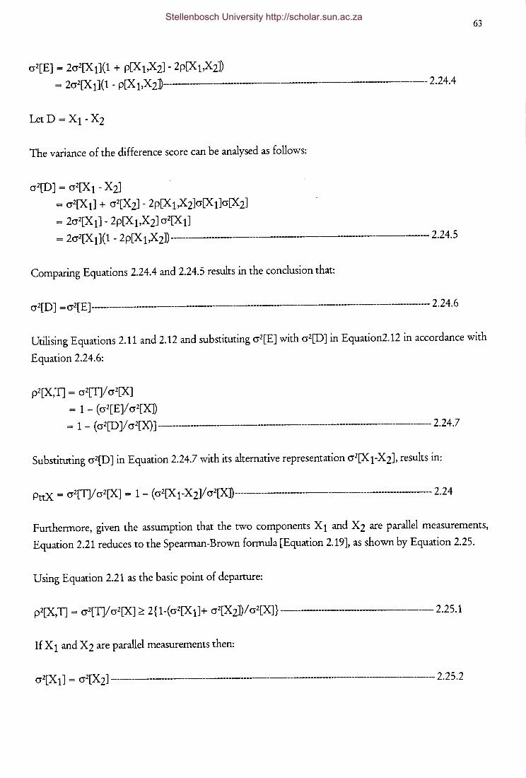
cr2[E] = 2cr2[X 1](1 + p[X 1X2J - 2p[X 1,X2]) = 2cr2[X 1](1 - p[X 1,X2]---------------------------------------------------- 2.24.4
LetD=X1-X2
The variance of the difference score can be analysed as follows:
cr2[D] = cr2[X 1- X2]
= cr2[X 1J + cr2[X2]- 2p[X 1X2]cr[X 1Jcr[X2]
= 2cr2[X 1J- 2p[X 1,X2] cr2[X 1J = 2cr2[X 1](1 - 2p[X 1X2J) ------------------------------------------------------ 2.24.5
Comparing Equations 2.24.4 and 2.24.5 results in the conclusion that:
cr 2[D] = cr2[E] ---------------------------------------------------------------------------------------------------------- 2. 2 4. 6
63
Utilising Equations 2.11 and 2.12 and substituting cr2[E] with cr2[D] in Equation2.12 in accordance with
Equation 2.24.6:
p2[X,T] = cr2[T]/ cr2[X]
= 1- (cr2[E]/cr2[X]) = 1 - ( cr2[D ]/ cr2[X)] ----------------------------------------------------------------------------------- 2.2 4.7
Substituting cr2[D] in Equation 2.24.7 with its alternative representation cr2[X 1-X2], results in:
PttX = cr2[T]/ cr2[X] = 1 - ( cr2[X 1-X 2]/ cr2[X]) ------------------------------------------------------------- 2.2 4
Furthermore, given the assumption that the two components X 1 and X 2 are parallel measurements,
Equation 2.21 reduces to the Spearman-Brown formula [Equation 2.19], as shown by Equation 2.25.
Using Equation 2.21 as the basic point of departure:
p2[X,T] = cr2[T]/ cr2[X] ~ 2 { 1-( cr2[X 1J+ cr2[X 2])/ cr2[X]} -------------------------------------- 2.25.1
If X 1 and X 2 are parallel measurements then:
cr 2 [X 1] = cr2[X 2J ------------------------------------------------------------------------------------------------------ 2. 2 5 . 2
Stellenbosch University http://scholar.sun.ac.za
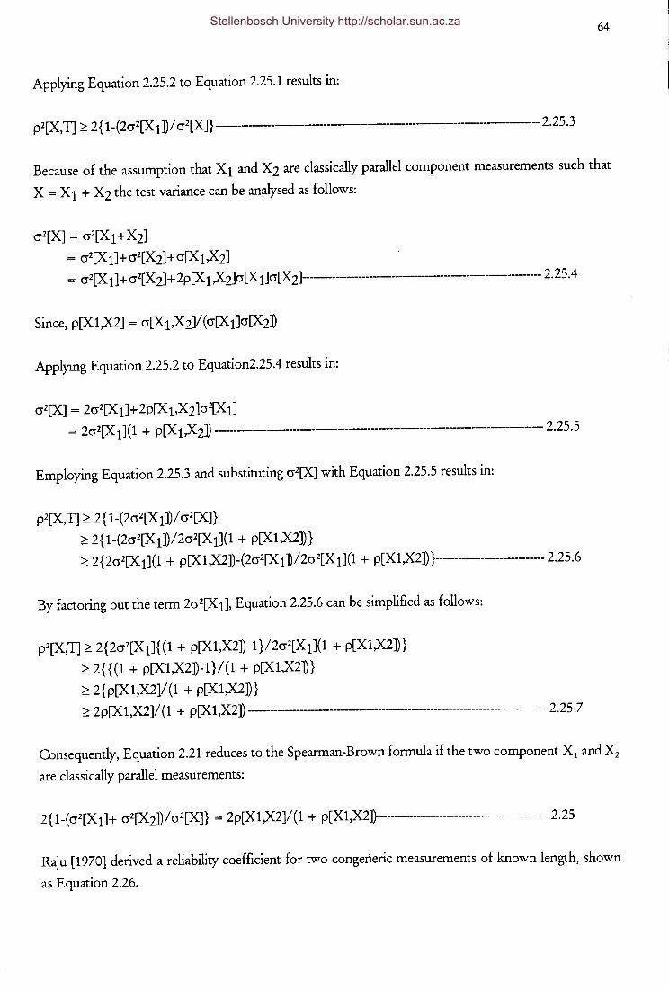
64
Applying Equation 2.25.2 to Equation 2.25.1 results in:
p2[X,11 ~ 2 { 1-(2cr2[X 1])/ cr2[X]} ------------------------------- ----2.25.3
Because of the assumption that X 1 and X2 are classically parallel component measurements such that
X = X 1 + X2 the test variance can be analysed as follows:
cr2[XJ = cr2[X 1 +X 2]
= cr2[X 1]+cr2[X2]+cr[X 1X2J = cr2[X 1]+ cr2[X 2]+ 2p[X 1 ,X 2]cr[X 1]cr[X 2]------------------------------------------ 2.25.4
Applying Equation 2.25.2 to Equation2.25.4 results in:
cr2[X] = 2cr2[X 1]+2p[X 1,X2]cr2[X 1J = 2cr2[X 1](1 + p[X 1X2D ------------------------------------------------------------- 2.25.5
Employing Equation 2.25.3 and substituting cr2[X] with Equation 2.25.5 results in:
p2[X,T] ~ 2{1-(2cr2[X1])/cr2[X]}
~ 2{1-(2cr2[X1])/2cr2[X1](1 + p[X1,XZ])} ~ 2{2cr2[X 1](1 + p[X1,XZ])-(2cr2[X 1])/2cr2[X 1](1 + p[X1,X2]) }------------------------ 2.25.6
By factoring out the term 2cr2[X 1J, Equation 2.25.6 can be simplified as follows:
p2[X,T] ~ 2{2cr2[X1]{(1 + p[X1,X2])-1}/2cr2[X1](1 + p[X1,XZ])}
~ 2{ {(1 + p[X1,X2])-1}/(1 + p[X1,X2])}
~ 2{p[X1,X2]/(1 + p[X1,X2])} ~ 2 p[X 1 ,X2]/ ( 1 + p[X 1 ,X2]) ------------------------------------------------------------ 2.25 .7
Consequently, Equation 2.21 reduces to the Spearman-Brown formula if the two component X 1 and X2
are classically parallel measurements:
2 { 1-( cr2[X 1] + cr2[X 2]) I cr2[X]} = 2p[X 1 ,XZ]/ ( 1 + p[X1 ,X2]}------------------------------------------- 2. 25
Raju [1970] derived a reliability coefficient for two congeneric measurements of known length, shown
as Equation 2.26.
Stellenbosch University http://scholar.sun.ac.za
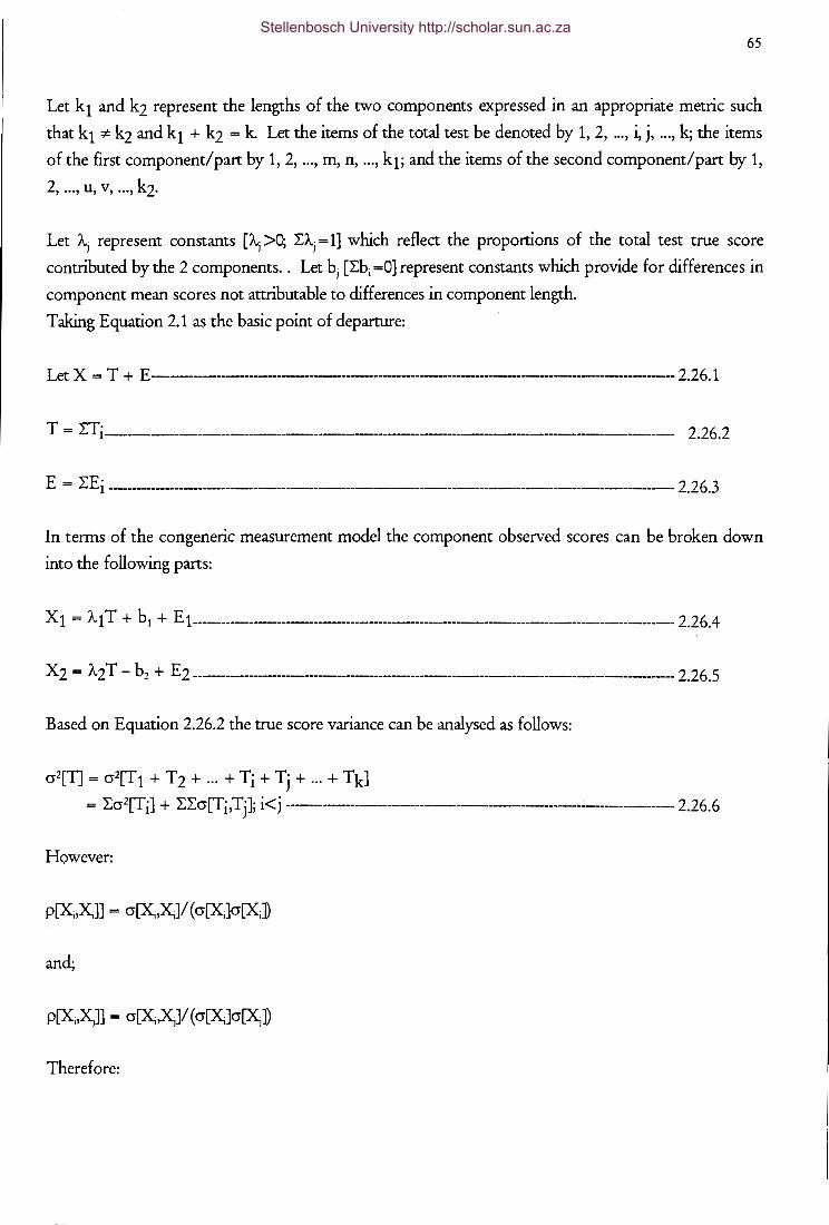
65
Let k1 and k2 represent the lengths of the two components expressed in an appropriate metric such
that k1 '¢ k2 and k1 + k2 = k. Let the items of the total test be denoted by 1, 2, ... , i, j, ... , k; the items
of the first component/part by 1, 2, ... , m, n, ... , k1; and the items of the second component/part by 1,
2, ... , u, v, ... , k2.
Let A; represent constants [A.; >0; LA;= 1] which reflect the proportions of the total test true score
contributed by the 2 components. . Let b; [Lbi =0] represent constants which provide for differences in
component mean scores not attributable to differences in component length.
Taking Equation 2.1 as the basic point of departure:
Let X = T + E------------------------------------------------------------- 2.26.1
T = LTi ----------------------------------------------------------------------------------- 2.26.2
E = LEi -------------------------------------------------------------------------------------------------------- 2 .26.3
In terms of the congeneric measurement model the component observed scores can be broken down
into the following parts:
X 1 = A 1 T + b I + E 1------------------------------------------------------------------------------------------------- 2.26. 4
X2 = "A2 T - bz + E2 --------------------------------------------------------------------------------------------- 2.26.5
Based on Equation 2.26.2 the true score variance can be analysed as follows:
cr2[T] = cr2[T 1 + T 2 + ... + Ti + Tj + ... + Tk]
= Lcr2[T i] + LLcr[T i,Tj]; i < j ---------------------------------------------------------------------- 2 .26. 6
However:
and;
Therefore:
Stellenbosch University http://scholar.sun.ac.za

66
cr[Xi,)\] = p[X,)\]cr[XJcr[XJ
and;
However:
and
Consequently:
The component true score variance and the component true score covariance terms in Equation 2.26.6
can therefore be substituted as follows:
cr2[T] = L:p[XiXiJcr[Ti]cr[Ti] + L:L:p[Xi,Xj]cr[fi]cr[fj]
= L:p[Xi,Xi]cr2[Ti] + L:L:p[XiXj]cr[fi]cr[fj]; (i< »---------------------------------------------------2.26.7
Let the k-item test now be split into two parts containing k 1 and k2 [k1:t:k2; k1 + k2 = k]items respectively.
Items in the first part are denoted by 1, 2, . . . ,n, m, . . . , k1; and the items in the second part are
denoted by 1, 2, ... ,u, v, ... , k2• Equation 2.26.7 can then be rewritten as:
cr2[T] = {L:p[Xn,Xn]cr2[T nJ+L:p[XuXu]cr2[fu]}+2{L:p[Xn,Xm]cr[T nJcr[T mJ
+ L:p[XwXv ]cr[T u]cr[T v ]+ L:p[XnXuJcr[f nJcr[T uU
= {k Ht(p[XnXnJcr2[T nD+ k2!l(P[XuXu]cr2[f u])}
+ {k 1 (k 1-1) !l(P[XnXmJcr[f nJcr[f mD + k2(k2-1) Jl(p[XwXv ]cr[T u]cr[T v ])
+ ( 2k 1 k 2) !l (p[Xn,Xu]cr[f nJcr[f uD}; ( n < m; u <v)-------------------------------------------------- 2 .26. 8
Stellenbosch University http://scholar.sun.ac.za
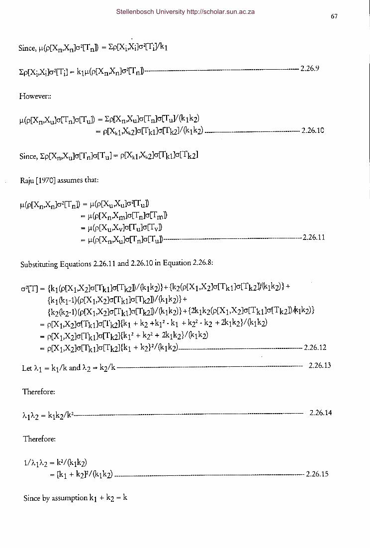
L:p[Xi,Xi]cr2[T iJ = k 1 ~ (p[X n Xn]cr2[T nD-------------------------------------------------------- 2 .26. 9
However::
~ (p[Xn,Xu]cr[T nJcr[T uJ) = L:p[XnXuJcr[f nJcr[f uJI (k 1 k V = p[Xk 1 A2]cr[fk1]cr[fk2]1 (k 1 k V ------------------------------------- 2.26.1 0
Raju [1970] assumes that:
~(p[Xn,Xn]cr2[T nJ) = ~(P[XuXu]cr2[f u]
= ~(p[XnXmJcr[f nJcr[f mD
= ~(p[XuXvJcr[fu]cr[fv] = ~(p[XnXu]cr[f nJcr[f uD----------------------------------------------------------- 2.26.11
Substituting Equations 2.26.11 and 2.26.10 in Equation 2.26.8:
cr2[T] = {k 1 (p[X 1 ,X 2]cr[Tk1]cr[Tk2]) I (k 1 k 2)} + {k2 (p[X 1 ,X 2Jcr[Tk 1Jcr[Tk2JY~1 k 2)} +
{k1 (k1-1) (p[X 1,X2]cr[fk1]cr[Tk2])l (k1 k2)} +
{k2(k2-1)(p[X 1,X2]cr[fk1]cr[fk2])l(k1 k2)} + {2k1 k2(p[X 1,X2]cr[Tk1]cr[Tk2J)~1kv} = p[X1,X2]cr[Tk1Jcr[Tk2]{k1 + k2 +k1 2
- k1 + ki- k2 + 2lqk2}l(k1k2)
= p[X1,X2]cr[Tk1]cr[Tk2]{k12 + ki + 2k1k2}l(k1k2)
= p[X 1 ,X 2Jcr[Tk 1]cr[Tk2] {k 1 + k 2} 2 I (k 1 k 2) ----------------------------------------------------------- 2.26.12
Let A1 = k1lk and A2 = k2lk ---------------------------------------------------------------------------------- 2.26.13
Therefore:
67
A 1 A 2 = k 1 k 21k2------------------------------------------------------------------------------------------------- 2. 26.14
Therefore:
11A1A2 = kZI(k1kv
= [k 1 + k 2J2 I (k 1 k 2) ---------------------------------------------------------------------------------------- 2. 2 6.15
Since by assumption k1 + k2 = k
Stellenbosch University http://scholar.sun.ac.za
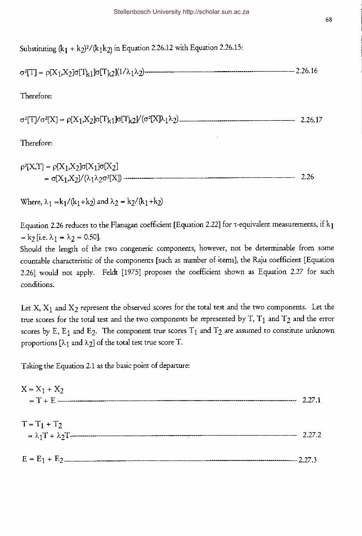
68
Substituting (lq + ki)2/(lqk2) in Equation 2.26.12 with Equation 2.26.15:
---------------------- 2.26.16
Therefore:
cr2[TJ/ cr2[X] = p[X 1 ,X 2Jcr[fk1]cr[fk2]/ ( cr2[X]A 1 A 2) ----------------------------- 2.26.17
Therefore:
p2[X,T] = p[X 1,X2]cr[X 1]cr[X2]
= cr[X 1 ,X 2J/ (A 1 A 2cr2[X]) --------------------------------------------------------------- 2.26
Equation 2.26 reduces to the Flanagan coefficient [Equation 2.22] fort-equivalent measurements, if k1
= k2 [i.e. A1 = A2 = 0.50].
Should the length of the two congeneric components, however, not be determinable from some
countable characteristic of the components [such as number of items], the Raju coefficient [Equation
2.26] would not apply. Feldt [1975] proposes the coefficient shown as Equation 2.27 for such
conditions.
Let X, X 1 and X2 represent the observed scores for the total test and the two components. Let the
true scores for the total test and the two components be represented by T, T 1 and T 2 and the error
scores by E, E 1 and E 2. The component true scores T 1 and T 2 are assumed to constitute unknown
proportions [A 1 and A 2J of the total test true score T.
Taking the Equation 2.1 as the basic point of departure:
X=X1 + X2 = T + E -------------------------------------------------------------------------:- 2.27.1
T=T1+T2 = A 1 T + A 2 T ---------------------------------------------------------------------------------- 2.27. 2
E = E 1 + E 2---------------------------------------------------------------------------------------------------- 2.27 .3
Stellenbosch University http://scholar.sun.ac.za
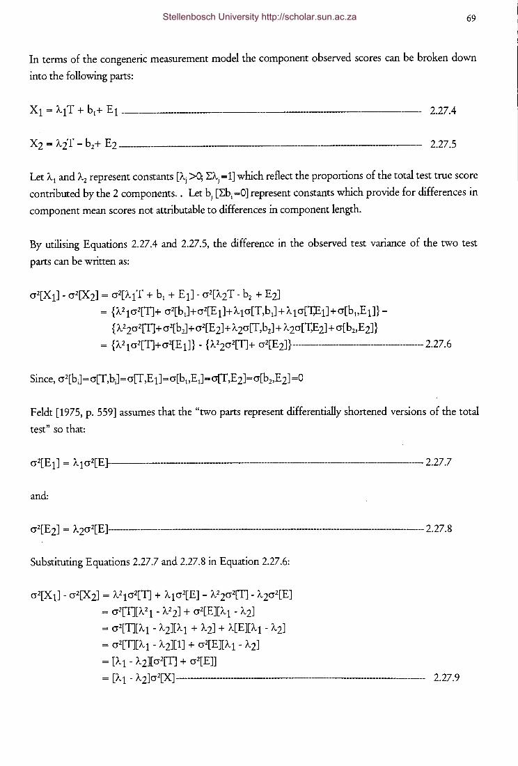
69
In terms of the congeneric measurement model the component observed scores can be broken down
into the following parts:
----------------------------- 2.27.4
X2 = A2 T - bz+ E2 --------------------------------------------- 2.27.5
Let A1 and A.z represent constants [A; >0; LA;= 1] which reflect the proportions of the total test true score
contributed by the 2 components. . Let b; [Lbi =0] represent constants which provide for differences in
component mean scores not attributable to differences in component length.
By utilising Equations 2.27.4 and 2.27.5, the difference in the observed test variance of the two test
parts can be written as:
cr2[Xt]- cr2[X2] = cr2[AtT + b1 + Et]- cr2[A2T- b2 + E2J
= {A2t cr2[T]+ cr2[b1]+cr2[Et]+At cr[T,b1] +At cr['I;Et]+cr[b1,Et]}
{A22cr2[T]+cr2[b2]+cr2[E2]+ A2cr[T,b2] + A2cr[T,E2J + cr[b2,E2]}
= {A21 cr2[TJ+cr2[E tJ} - {A22cr2[T]+ cr2[E2]}----------------------------------------- 2.27.6
Feldt [1975, p. 559] assumes that the "two parts represent differentially shortened versions of the total
test" so that:
cr2[E 1] = A 1 cr2[E ]----------------------------------------------------------------------------- 2.27 .7
and:
cr2[E 2J = A 2cr2[E ]----------------------------------------------------------------------------------- 2.27. 8
Substituting Equations 2.27.7 and 2.27.8 in Equation 2.27.6:
cr2[X tJ - cr2[X2] = A21 cr2[TJ + At cr2[E]- A22cr2[TJ- A2cr2[E]
= cr2[TJ(A21 - A22] + cr2[E][At - A2]
= cr2[T][At - A2][Al + A2] + A[E][At - A2]
= cr2[T][At - A2][1] + cr2[E][At - A2]
=[At- A2][cr2[TJ + cr2[E]]
= [A 1 - A 2]cr2[X] ----------------------------------------------------------------------- 2. 27.9
Stellenbosch University http://scholar.sun.ac.za

Expressing Equation 2.27.9 in terms of the observed test variance of the total test:
cr2[X 1]- cr2[X2])1 cr2[XJ = ([A1 - A2]cr2[X]I cr2[XJ
= [A1 - A2] --------------- ·--- 2.27.10
However by definition:
A1 + A2 = 1------------------------------------------2.27.11
Isolating A1 in Equation 2.27.11:
A 1 = 1 - A 2 ------------------------------------------------------------------------------------------ 2.27.12
Substituting Equation 2.27.12 in Equation 2.2710:
(cr2[X1]- cr2[X2J)Icr2[X] = (1- AV- A2 = 1- 2A 2 ---------------------------------------------------- 2.27.13
Isolating 2A2 in Equation 2.27.13:
2A 2 = 1 - { ( cr2[X 1J - cr2[X 2] I cr2[X]} = { cr2[X] - ( cr2[X 1J - cr2[X 2]} I cr2[X]--------------------------------------------------------------- 2.27.14
Therefore:
A 2 = { cr2[X] - ( cr2[X 1] - cr2[X 2J)} I 2cr2[X]-------------------------------------------------------------- 2.27.15
Similarly by substituting A2 = 1 - A1 in Equation 2.27.10:
A 1 = { cr2[X] + ( cr2[X 1J - cr2[X 2J) } I 2cr2[X}--------------------------------------------------------- 2.27.17
However:
cr[X 1,X2J = cr[(f1+E1),(f2 +E~] = cr[T1T2+ T1E2 +E1T2 +E1E2]
= cr[Tt,TzJ
= cr[AtT,AzTJ
= A1Ap[T,T]
70 Stellenbosch University http://scholar.sun.ac.za
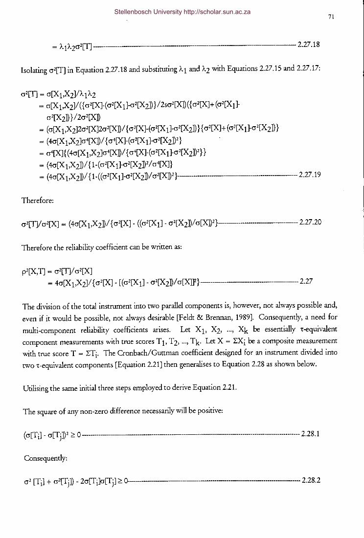
= A 1 A 2 cr2[T] ---------------------------------------------------------------------------- 2.27.18
Isolating cr2[T] in Equation 2.27.18 and substituting A1 and A2 with Equations 2.27.15 and 2.27.17:
cr2[T] = cr[X 1,X2]1A1 A2
= cr[X 1 ,X 2JI ( { cr2[XJ-( cr2[X 1J-cr2[X 2J)} I 2scr2[X]) ( { cr2[X]+ ( cr2[X 1J-
cr2[X 2J)} I 2cr2[X])
= (cr[X 1,X2]2cr2[X]2cr2[X])I { cr2[XJ-(cr2[X 1J-cr2[X2]) }{ cr2[X]+ (cr2[X 1J-cr2[X2J)}
= (4cr[X 1,X2]cr4[X])I { cr4[XJ-(cr2[X 1J-cr2[X2])2}
= cr4[X]{ (4cr[X 1,X2Jcr4[X])I { cr4[XJ-(cr2[X 1J-cr2[X2])2}}
= (4cr[X 1,X2J)I { 1-( cr2[X 1J-cr2[X2]2I cr4[XJ}
= ( 4cr[X 1 ,X 2J) I { 1-( ( cr2[X 1J-cr2[X 2D I cr2[X])2 }---------------------------------------------------- 2.27.19
Therefore:
Therefore the reliability coefficient can be written as:
pz[X,T] = cr2[T]I cr2[XJ
= 4cr[X 1 ,X 2JI { cr2[X] - [ ( cr2[X 1J - cr2[X 2J) I cr[X]]2} ----------------------------------------- 2.27
71
The division of the total instrument into two parallel components is, however, not always possible and,
even if it would be possible, not always desirable [Feldt & Brennan, 1989]. Consequently, a need for
multi-component reliability coefficients arises. Let X b X2, ... , Xk be essentially 't-equivalent
component measurements with true scores T1, T2, ... , Tk. Let X= L:Xi be a composite measurement
with true score T = L:Ti. The CronbachiGuttman coefficient designed for an instrument divided into
two 't-equivalent components [Equation 2.21] then generalises to Equation 2.28 as shown below.
Utilising the same initial three steps employed to derive Equation 2.21.
The square of any non-zero difference necessarily will be positive:
( cr[Ti] - cr[Tj])2 ~ 0 ----------------------------------------------------------------------------------------------------- 2.28.1
Consequently:
cr2 [Ti] + cr2[Tj]) - 2cr[Ti]cr[Tj] ~ 0------------------------------------------------------------------------- 2.28.2
Stellenbosch University http://scholar.sun.ac.za
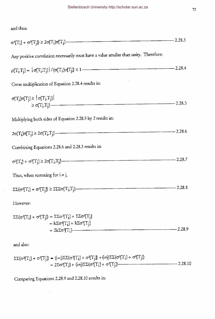
and thus:
cr2[Ti] + cr2[Tj]) ~ 2cr[Ti]cr[Tj] --------------------------------- 2.28.3
Any positive correlation necessarily must have a value smaller than unity. Therefore:
p[Ti,Tj] = I cr[Ti,Tj] I /(cr[Ti]cr[fj] s 1----------------------------------2.28.4
Cross multiplication of Equation 2.28.4 results in:
cr[Ti]cr[Tj] ~ I cr[Ti,Tj] I ~ cr[T i,Tj] ---------------------------------------------------------------------------------- 2.28. 5
Multiplying both sides of Equation 2.28.5 by 2 results in:
2cr[T i]cr[Tj] ~ 2cr[T i' Tj] ---------------------------------------------------------------------------- 2.2 8. 6
Combining Equations 2.28.6 and 2.28.3 results in:
cr2[T i] + cr2[Tj] ~ 2cr[Ti, Tj] ------------------------------------------------------------------------------------- 2.2 8.7
Thus, when summing fori =F j,
I: I: ( cr2[Ti] + cr2[Tj]) ~ 2I:I:cr[T i,Tj}---------------------------------------------------------------- 2. 28.8
However:
I: I:( cr2[Ti] + cr2[Tj]) = I:I:cr2[Ti] + I:I:cr2[Tj]
= Ucr2[Ti] + kLcr2[Tj] = 2ki:cr2[T i}------------------------------------------------------- 2.28. 9
and also:
I:I:(cr2[Ti] + cr2[Tj]) = (i=j)I:I:(cr2[Ti] + cr2[Tj] +(i=Fj)I:I:(cr2[Ti] + cr2[Tj]) = 2I:cr2[Ti] + (i=Fj)I:I:( cr2[Ti] + cr2[Tj])---------------------------------------------- 2.28.10
Comparing Equations 2.28.9 and 2.28.10 results in:
72 Stellenbosch University http://scholar.sun.ac.za
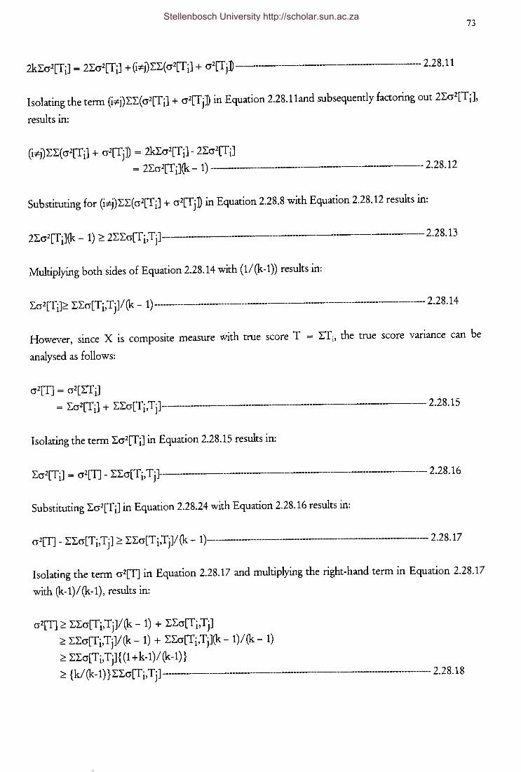
73
2k:Ecr2[Ti] = 2:Ecr2[Ti] + (i:;ej) :E:E( cr2[T iJ + cr2[Tj] --------------------------------------- 2.28.11
Isolating the term (i:;ej):E:E(cr2[Ti] + cr2[Tj] in Equation 2.28.11and subsequently factoring out 2:Ecr2[Ti],
results in:
(i:;ej):E:E(cr2[Ti] + cr2[Tj]) = 2kLcr2[TiJ- 2:Ecr2[Ti] = 2:Ecr2[Ti](k- 1) -----------------------------------------------2.28.12
Substituting for (i:;ej):E:E(cr2[TiJ + cr2[Tj] in Equation 2.28.8 with Equation 2.28.12 results in:
2:Ecr2[Ti](k- 1) ~ 2:E:Ecr[Ti,Tj]------------------------------------------- 2.28.13
Multiplying both sides of Equation 2.28.14 with (1/(k-1)) results in:
:Ecr2[Ti]~ :E:Ecr[Ti,T j]/ (k - 1) -------------------------------------------------------------------------------------- 2. 28.14
However, since X is composite measure with true score T = :ETi, the true score variance can be
analysed as follows:
cr2[T] = cr2[:ETi] = :Ecr2[T iJ + :E:Ecr[Ti, Tj]-------------------------------------------------------------------------------- 2. 2 8.15
Isolating the term :Ecr2[Ti] in Equation 2.28.15 results in:
:Ecr2[T iJ = cr2[T] - :E:Ecr[Ti, T jJ------------------------------------------------------------------------------ 2. 28.16
Substituting :Ecr2[Ti] in Equation 2.28.24 with Equation 2.28.16 results in:
cr2[T] - :E:Ecr[Ti,Tj] ~ :E:Ecr[T i ,Tj]/ (k - 1 )------------------------------------------------------------------- 2.28.17
Isolating the term cr2[T] in Equation 2.28.17 and multiplying the right-hand term in Equation 2.28.17
with (k-1)/ (k-1), results in:
cr2[T] ~ :E:Ecr[Ti,Tj]/ (k- 1) + :E:Ecr[Ti,Tj]
~ :E:Ecr[Ti,Tj]/(k- 1) + :E:Ecr[Ti,Tj](k- 1)/(k- 1)
~ :E:Ecr[Ti,Tj]{ (1 +k-1)/(k-1)} ~ {k/ (k -1)} :E:Ecr[T i' T j] ------------------------------------------------------------------------------------ 2. 2 8.18
Stellenbosch University http://scholar.sun.ac.za
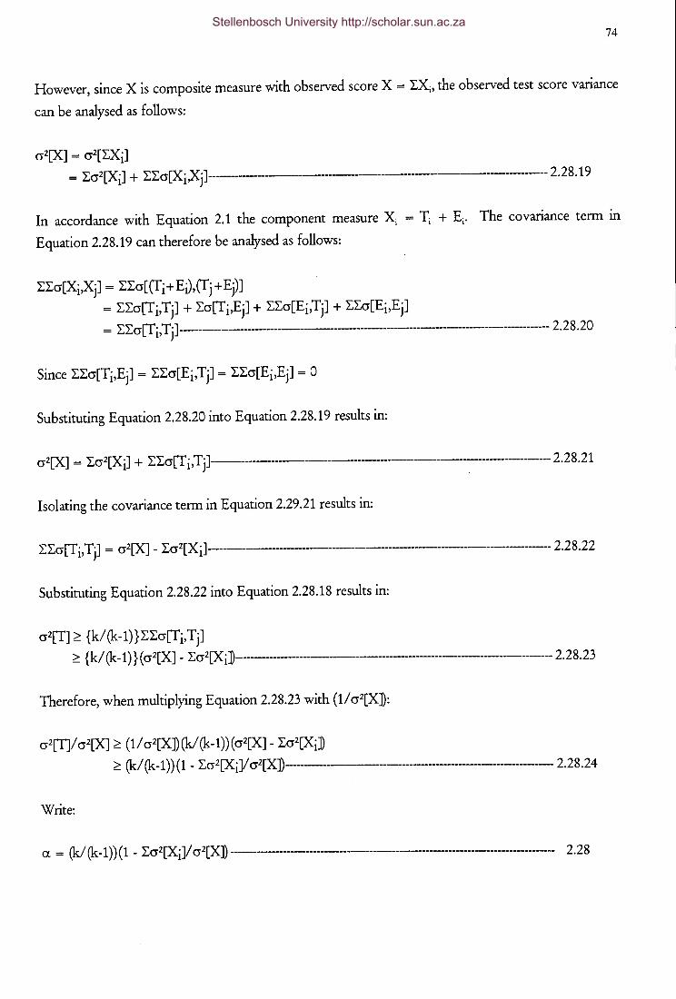
74
However, since X is composite measure with observed score X = :LXi, the observed test score variance
can be analysed as follows:
cr2[X] = cr2[:LXi] = :Lcr2[Xi] + :L:Lcr[Xi,Xj}-------------------------------------------------- 2.28.19
In accordance with Equation 2.1 the component measure Xi = Ti + Ei. The covariance term in
Equation 2.28.19 can therefore be analysed as follows:
:L:Lcr[Xi,Xj] = :L:Lcr[(fi+EJ,(fj+Ej)]
= :L:Lcr[Ti,Tj] + :Lcr[Ti,Ej] + :L:Lcr[Ei,Tj] + :L:Lcr[Ei,Ej]
= :L:Lcr[T i' Tj] -------------------------------------------------------------------------------- 2.2 8.20
Substituting Equation 2.28.20 into Equation 2.28.19 results in:
cr2[X] = :Lcr2[Xi] + :L:Lcr[T i,Tj}-------------------------------------------------------------------- 2.2 8.21
Isolating the covariance term in Equation 2.29.21 results in:
:L:Lcr[Ti, Tj] = cr2[X] - :Lcr2[Xi}---------------------------------------------------------------------------- 2.2 8.22
Substituting Equation 2.28.22 into Equation 2.28.18 results in:
cr2[T] ~ {k/(k-1)}:L:Lcr[Ti,Tj] ~ {k/ (k -1)} ( cr2[X] - :Lcr2[Xi]------------------------------------------------------------------------ 2.2 8.23
Therefore, when multiplying Equation 2.28.23 with (1/ cr2[X]):
cr2[T]/cr2[X] ~ (1/cr2[X])(k/(k-1))(cr2[X]- :Lcr2[Xi]
~ (k/ (k -1)) ( 1 - :Lcr2[Xi]/ cr2[X]) ------------------------------------------------ 2.28 .2 4
Write:
a = (k/ (k -1)) ( 1 - :Lcr2[Xi]/ cr2[X]) -------------------------------------------------------------------------- 2.28
Stellenbosch University http://scholar.sun.ac.za
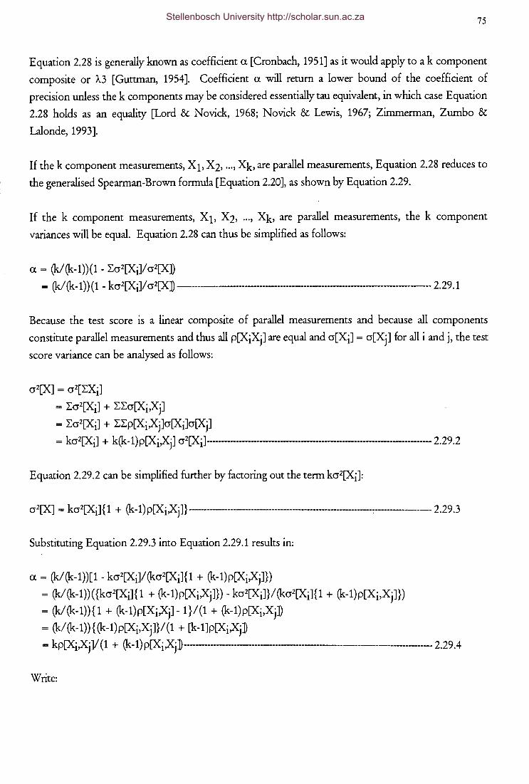
75
Equation 2.28 is generally known as coefficient a [Cronbach, 1951] as it would apply to a k component
composite or A.3 [Guttman, 1954]. Coefficient a will return a lower bound of the coefficient of
precision unless the k components may be considered essentially tau equivalent, in which case Equation
2.28 holds as an equality [Lord & Novick, 1968; Novick & Lewis, 1967; Zimmerman, Zumbo &
Lalonde, 1993].
If the k component measurements, X 1, X2, ... , Xk, are parallel measurements, Equation 2.28 reduces to
the generalised Spearman-Brown formula [Equation 2.20], as shown by Equation 2.29.
If the k component measurements, X 1, X2, ... , Xk, are parallel measurements, the k component
variances will be equal. Equation 2.28 can thus be simplified as follows:
a= (k/(k-1))(1- Lcr2[Xi]/cr2[X])
= (kl (k -1)) ( 1 - kcr2[Xi]/ cr2[X] ------------------------------------------------------------------ 2. 29.1
Because the test score is a linear composite of parallel measurements and because all components
constitute parallel measurements and thus all p[XiXj] are equal and cr[Xi] = cr[Xj] for all i and j, the test
score variance can be analysed as follows:
cr2[X] = cr2[LXi]
= Lcr2[Xi] + LLcr[Xi,Xj]
= Lcr2[Xi] + LLP[Xi,Xj]cr[Xi]cr[Xj]
= kcr2[Xi] + k(k -1) p[XiXj] cr2[Xi}---------------------------------------------------------------------- 2.29 .2
Equation 2.29.2 can be simplified further by factoring out the term kcr2[XiJ:
cr2[X] = kcr2[Xi] { 1 + (k -1) p[XiXj]} ---------------------------------------------------------------------- 2. 29.3
Substituting Equation 2.29.3 into Equation 2.29.1 results in:
a= (k/(k-1))[1- kcr2[Xi]/(kcr2[Xi]{1 + (k-1)p[XiXj]})
= (k/(k-1))({kcr2[Xi]{1 + (k-1)p[XiXj]})- kcr2[Xi]}/(kcr2[Xi]{1 + (k-1)p[Xi,Xj]})
= (k/(k-1)){1 + (k-1)p[Xi,Xj]- 1}/(1 + (k-1)p[Xi,Xj])
= (kl(k-1)){(k-1)p[Xi,Xj]}/(1 + [k-1Jp[XiXjD
= kp[Xi,Xj]/ ( 1 + (k -1) p[XiXj D ------------------------------------------------------------------------- 2.29 .4
Write:
Stellenbosch University http://scholar.sun.ac.za
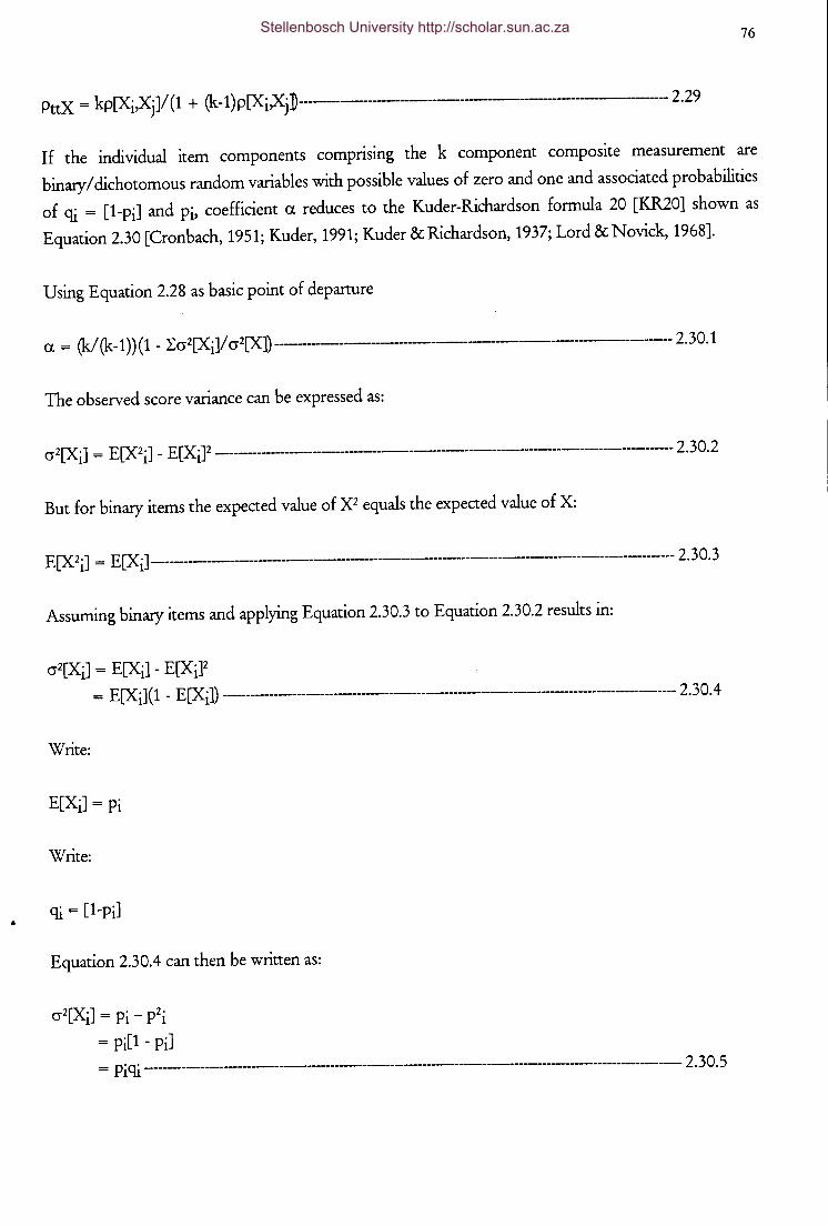
..
76
PttX = kp[Xi,Xj]/(1 + (k-1)p[XiXj]---------------- ----------- 2.29
If the individual item components comprising the k component composite measurement are
binary/dichotomous random variables with possible values of zero and one and associated probabilities
of qj = [1-pi] and pi, coefficient a reduces to the Kuder-Richardson formula 20 [KR20] shown as
Equation 2.30 [Cronbach, 1951; Kuder, 1991; Kuder & Richardson, 1937; Lord & Novick, 1968].
Using Equation 2.28 as basic point of departure
a = (kl (k -1)) ( 1 - :l:cr2[XiJ/ cr2[X]) --------------------------------------------- 2.30.1
The observed score variance can be expressed as:
cr2[Xi] = E[X2i] - E[Xi]2 --------------------------------------------------------------------------------- 2.30.2
But for binary items the expected value of X2 equals the expected value of X:
E[X2 i] = E[Xi] ------------------------------------------------------------------------------------------ 2. 3 0. 3
Assuming binary items and applying Equation 2.30.3 to Equation 2.30.2 results in:
cr2[Xi] = E[Xi] - E[Xi]2 = E[Xi]( 1 - E[Xi]) --------------------------------------------------------------------------------- 2. 3 0. 4
Write:
E[Xi] =Pi
Write:
Equation 2.30.4 can then be written as:
cr2[Xi] = Pi - P2 i
= Pi[l- Pi] = Pi qj ------------------------------------------------------------------------------------------------------ 2. 30. 5
Stellenbosch University http://scholar.sun.ac.za
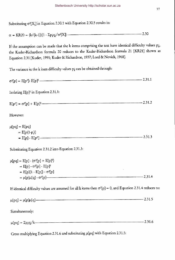
77
Substituting cr2[Xi] in Equation 2.30.1 with Equation 2.30.5 results in:
a= KR20 = (k/(k-1))(1- Lpiq/cr2[X] --------------------------------------------------2.30
If the assumption can be made that the k items comprising the test have identical difficulty values Pi'
the Kuder-Richardson formula 20 reduces to the Kuder-Richardson formula 21 [KR21] shown as
Equation 2.31 [Kuder, 1991; Kuder & Richardson, 1937; Lord & Novick, 1968].
The variance in the k item difficulty values Pi can be obtained through:
cr2[p] = E[p2]- E[p ]2 ----------------------------------------------------------- 2.31.1
Isolating E[p ]2 in Equation 2.31.1:
E[p2] = cr2[p] + E[p ]2 ---------------------------------------------------------------------------------- 2.31.2
However:
~[pq] = E[pq]
= E[p(1-p)]
= E[p] - E[p2] ----------------------------------------------------------------------------------------- 2.31.3
Substituting Equation 2.31.2 into Equation 2.31.3:
~[pq] = E[p] - ( cr2[p] + E[p ]2)
= E[p]- cr2[p]- E[p]2
= E[p](1- E[p])- cr2[p]
= ~[p ]~[ q] - cr2[p ]---------------------------------------------------------------------------------- 2.31. 4
If identical difficulty values are assumed for all k items then cr2[p] = 0, and Equation 2.31.4 reduces to:
~[pq] = ~[p ]~[ q]---------------------------------------------------------------------------------- 2.31.5
Simultaneously:
~[pq] = L pi qi/k ------------------------------------------------------------------------------------------------------- 2. 31.6
Cross multiplying Equation 2.31.6 and substituting ~[pq] with Equation 2.31.5:
Stellenbosch University http://scholar.sun.ac.za

78
:Epi<Ji = k!l[pq] = k!l[P ]!l[ q]------------------------------------------------------ 2.31.7
Substituting in Equation 2.30 with Equation 2.31.7:
a = KR20 = (k/ (k -1)) ( 1 - k!l[P ]!l[ q]/ cr2[X]) ------------------------------------- 2.31. 8
Consequently, if identical difficulty values are assumed for all k items:
KR20 = KR21 = (k/ (k-1)) (1 - k!l[P ]!l[ q]/ cr2[X]}---------------------------- 2.31
To the extent that the assumption of identical Pi-values is in fact not satisfied, the KR21 is negatively
biased. Tucker [1949] presented an equation to correct for the underestimation of KR20 shown as
Equation 2.32.
Using Equation 2.26 as point of departure:
KR20 = (k/(k-1))(1 - :E Piq/ cr2[X])
According to Equation 2.31.4 and Equation 2.31.6:
!l[ Pi<Ji] = !l[Pi]!l[ <Ji] - cr2[Pi] = :Epi <Jilk ---------------------------------------------------------------------------------------------- 2. 3 2.1
Thus, if non-identical difficulty values are assumed for all k items:
:Epi<Ji = k!l[Pi<Ji]
= k[!l[Pi]!l[ <Ji] - cr2[Pi]
= k!l[Pi]!l[ q] - kcr2[p i] ----------------------------------------------------------------------- 2.3 2. 2
Thus, by inserting Equation 2.32.2 into Equation 2.26:
KR20 = (k/(k-1))(1- {k!l[Pi]!l[<Ji]- kcr2[pi]}/cr2[X]) = (k/(k-1))(1- {k!l[Pi]!l[<Ji]lcr2[X]})- ((k/(k-1))(kcr2[pi])/cr2[X]) = (k/ (k-1))(1 - k!l[Pi]!l[<Ji]l cr2[X]) - ((k2cr2[pi])/ (k-1)cr2[X]---------------------------------- 2.32.3
Consequently, if non-identical difficulty values are assumed for all k items the following correction
applies:
Stellenbosch University http://scholar.sun.ac.za
79
KR20 = KR21 + k2cr2[pi]/(k-1)cr2[X}----------------------- ----------------2.32
Another reliability coefficient based on more than two t-equivalent components was suggested by
Guttman [1945]. Like Cronbach's a and the Kuder-Richardson formula, Guttman's A-2 returns a lower
bound to the reliability of a measure [Cronbach, 1951; Guttman, 1954; Kuder &Richardson, 1937; ten
Berge & Zegers, 1978]. The Guttman reliability coefficient A-2 is shown as Equation 2.33.
A-2 = (LLcr[Xi,Xj] + {kl (k-1)LL(i=t=j)cr2[Xi,Xj]} ~)/ cr2[X]
= ((cr2[X]- Lcr2[Xi]) + {kl(k-1)LL(i=t=j)cr2[Xi,Xj]} ~)/cr2[X}---.:----------------------- 2.33
If Equation 2.33 does provide a lower bound to the reliability coefficient, then:
A2 ~ p2[X,T]
~ cr2[T]/ cr2[X] --------------------------------------------------------------------------------------------------- 2. 3 3 .1
Substituting Equation 2.33 in Equation 2.33.1 and isolating cr2[T]:
cr2[T] ~ { ((cr2[X]- Lcr2[Xi]) + {k/ (k-1)LL(i=t=j)cr2[Xi,Xj]} ~)/ cr2[XJ}cr2[X]
~ LLO"[Xi,Xj] + {k/ (k -1) LLcr2[Xi,Xj]} ~ ------------------------------------------------ 2.3 3.2
Rearranging the terms in Equation 2.33.2:
cr2[T] - LLcr[Xi,Xj] ~ (k/ (k -1) LLcr2[Xi,Xj] ~---------------------------------------------------------- 2. 3 3. 3
However:
cr2[T] = cr2[LTi]
= Lcr2[T i] + LLcr[Xi,Xj] ------------------------------------------------------------------------------- 2. 3 3. 4
Isolating the term Lcr2[Ti] in Equation 2.33.4:
Lcr2[Ti] = cr2[T]- LLcr[Xi,Xj]------------------------------~-------------------- 2.33.5
Therefore, by substituting Equation 2.33.5 in Equation 2.33.3 and if Equation 2.33 does provide a
lower bound to the reliability coefficient, then:
Lcr2[T i] ~ (k/ (k -1) LLcr2[Xi,Xj] ~-------------------------------------------------------------------------------- 2. 3 3. 6
Stellenbosch University http://scholar.sun.ac.za
Furthermore, because any non-zero squared difference necessarily must be positive:
(cr2[Ti]- cr2[Tj])2;::: 0------------------------------------ 2.33.7
Therefore:
----------------------2.33.8
Therefore:
------------------------2.33.9
However, since -1~p[Ti,Tj];:::1:
p2[Ti,Tj] = cr2[Ti,Tj]/ ( cr2[Ti]cr{Tj] ~ 1--------------------------------------------------- 2.33.10
Equation 2.33.10 can only be true if:
cr2[T i]cr2[Tj] ;::: cr2[T i' Tj] ---------------------------------------------------------------------- 2.3 3 .11
Multiplying Equation 2.33.11 by 2:
2cr2[Ti] cr2[Tj] ;::: 2cr2[Ti,Tj}------------------------------------------------------------ 2.3 3.12
Combining Equations 2.33.9 and 2.33.12:
--------------------------------------- 2.33.13
Thus, if summing fori* j:
LL[ cr4[Ti] + cr4[Tj]] ;::: 2LLcr2[Ti,Tj}------------------------------------- 2.33.14
However:
LL[ cr4[Ti] + cr4[Tj]] = LLcr4[Ti] + LLcr4[Tj]]
= kcr4[Ti] + kLcr4[Tj]
= 2kLcr4[T iJ------------------------------------------------------------------ 2.3 3 .15
80 Stellenbosch University http://scholar.sun.ac.za
The left hand term in Equation 2.33.15 can, however, also be written as:
Z:Z:[cr4[Ti] + cr4[Tj]] = Z:Z:(i=j)(cr4[Ti] + cr4[Tj] + Z:Z:(i:t:j)(cr4[Ti] + cr4[Tj])
= 2Z:cr4[Ti] + Z:Z:(i:t:j)(cr4[Ti] + cr4[Tj])-------- ----- 2.33.16
Substituting Equation 2.33.15 in Equation 2.33.16:
Isolating Z:Z:(i:t:j)(cr4[Ti] + cr4[Tj] in Equation 2.33.17 and factoring out the term 2:l:cr4[TiJ:
Z:Z:(i:t:j)(cr4[Ti] + cr4[Tj]) = 2k:l:cr4[Ti]- 2:l:cr4[Ti] = 2:l:cr4[T i](k - 1) ------------------------------------------------------------------ 2.3 3 .18
Combining Equations 2.33.13 and 2.44.18:
2:l:cr4[T i] (k - 1) ~ 2:l::l:cr2[T i ,Tj}----------------------------------------------------------------------------------- 2. 3 3.19
Isolating the term :l:cr4[Ti] in Equation 2.33.19:
Z:cr4[T i] ~ :l::l:cr2[T i•Tj]/ (k - 1) -------------------------------------------------------------------------------- 2. 3 3 .20
However:
(Z:cr2[Ti])2 = Z:cr4[Ti] + Z::l:cr2[T i]cr2[TjJ------------------------------------------------------------------ 2.3 3. 21
Therefore, by rearranging the terms of Equation 2.33.21 and by utilising Equation 2.33.11
(Z:cr2[Ti])2 - :l:cr4[Ti] = :l::l:cr2[Ti]cr2[Tj]
~ :l::l:cr2[Ti,Tj]
~:l::l:cr2[Xi.Xj] ------------------------------------------------------------------ 2. 3 3.22
Since :l::l:cr2[X· X] = :l::l:cr2[T· T] 1• J 1• J
Isolating the term (Z:cr2[Ti])2 in Equation 2.33.22:
(Z:cr2[T i])2 ~ Z:cr4[T i] + LLcr2[Xi.Xj] ------------------------------------------------------------------------------ 2. 3 3 .23
81 Stellenbosch University http://scholar.sun.ac.za
Substituting Equation 2.33.20 in Equation 2.33.23 and multiplying the term ~~cr2[Xi,Xj] v.ith
(k- 1)/ (k-1):
(Lcr2[Ti])2 ~ L~cr2[Ti,Tj]/ (k- 1) + ~~cr2[XiXj]
~ ~~cr2[Ti,Tj]/(k- 1) + (k-1)~~ cr2[XiXj]/(k-1)
~ ~~cr2[XiXj](1+k-1)/(k-1)
~ ~~cr2[XiXj](k/ (k -1)) ------------------------------------------------------------------ 2. 3 3. 2 4
82
Consequently, since Equation 2.33.24 is identical to Equation 2.33.6 derived from Guttman's "-2
formula:
"-2 = (L~cr[Xi,Xj] + {k/(k-1)~~cr2[XiXj]}lh)/cr2[X] ~ cr2[T]/ cr2[X] ---------------------------------------------------------------------------------------------------- 2. 3 3
According to Feldt and Brennan [1989], Equation 2.33 equals the Cronbach a in the parameter, if the
assumption of essential 't-equivalence holds for all components. The probability of exact equality on
sample data, however, seems low [Feldt & Brennan, 1989]. Lord and Novick [1968] reconunend the
use of Guttman's A.2 when some of the test items have negative inter-correlations.
Gilmer and Feldt [1983] derived a reliability coefficient for multiple congeneric measurements. The
Gilmer and Feldt reliability coefficient is shown as Equation 2.34.
Assume w congeneric components. Let the lengths of the components be k1, ... , ki, , kw; k
representing the number of items in the component. Therefore, in accordance with the classical
measurement model:
X= [T + E]
E = [E1 + E2 + ··· + £w]
Let \ represent constants [\ >0; L\ = 1] which reflect the proportions of the total test true score
contributed by the w components. Let bi [:Lb; =0] represent constants which provide for differences in
Stellenbosch University http://scholar.sun.ac.za
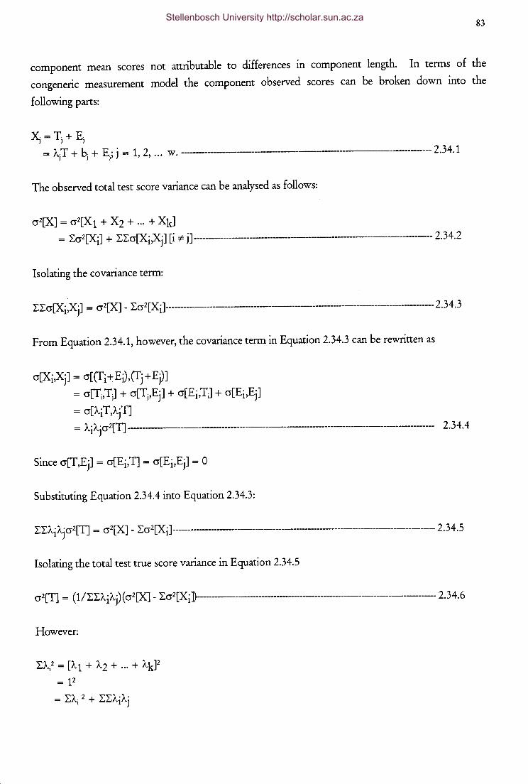
83
component mean scores not attributable to differences in component length. In terms of the
congeneric measurement model the component observed scores can be broken down into the
following parts:
Y.=T+E "') J J
= A.iT + bi + Ei; j = 1, 2, ... w. ----------------------------------------- 2.34.1
The observed total test score variance can be analysed as follows:
cr2[X] = cr2[X 1 + X2 + ... + Xk]
= ~cr2[Xi] + ~~cr[XiXjJ [i * j] ------------------------------------------------------------------------- 2.34.2
Isolating the covariance term:
~~cr[Xi,Xj] = cr2[X] - ~cr2[XiJ-------------------------------------------------------------------------------------- 2.34. 3
From Equation 2.34.1, however, the covariance term in Equation 2.34.3 can be rewritten as
cr[Xi,Xj] = cr[(fi+EJ,(fj+Ej)]
= cr[Ti,Ti] + cr[Ti,Ej] + cr[Ei,TJ + cr[Ei,Ej]
= cr[A.iT,A.jTJ
= "-i Aj cr2[T] --------------------------------------------------------------------------------------------------- 2. 3 4. 4
Substituting Equation 2.34.4 into Equation 2.34.3:
~~"-i "-jcr2[T] = cr2[X] - ~cr2[Xi] ---------------------------------------------------------------------------------- 2.34 .5
Isolating the total test true score variance in Equation 2.34.5
cr2[T] = ( 1 ~~~"-i "-j) ( cr2[X] - ~cr2[Xi]----------------------------------------------------------------------- 2. 3 4. 6
However:
~\2 = [A.1 + "-2 + ... + "-k]2
=F
= ~A.i 2 + ~~"-i"-j
Stellenbosch University http://scholar.sun.ac.za
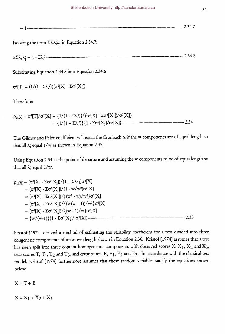
84
= 1------------------------------------- --------·-- --- 2.34.7
Isolating the term l:l:A.i"'-j in Equation 2.34.7:
l:l:A.i"'-j = 1 - l:\2 ------------------------------------------------------------------- 2.34.8
Substituting Equation 2.34.8 into Equation 2.34.6
Therefore:
PttX = cr2[TJ/ cr2[XJ = { 1/ ( 1 - l:A.i2) }{ ( cr2[XJ - l:cr2[Xi])/ cr2[X]}
= { 1/ ( 1 - l:A.i2) }{ 1 - l:cr2[Xi]/ cr2[X]} ------------------------------------- 2.34
The Gilmer and Feldt coefficient will equal the Cronbach a if the w components are of equal length so
that all "'-i equall/w as shown in Equation 2.35.
Using Equation 2.34 as the point of departure and assuming the w components to be of equal length so
that all "'-i equal1/w:
PttX = (cr2[X]- l:cr2[Xi])/(1- l:A.2I)cr2[X]
= (cr2[X]- l:cr2[Xi])/(1- w/w2)cr2[X]
= (cr2[XJ- l:cr2[Xi])/ { (w2- w)/w2}cr2[XJ
= (cr2[X]- l:cr2[Xi])/ { (w(w- 1))/w2}cr2[X]
= (cr2[XJ- l:cr2[Xi])/ { (w- 1)/w }cr2[X]
= { w I (w -1) }( 1 - l:cr2[Xi]/ cr2[X]) ------------------------------------------------------ 2. 3 5
Kristof [1974] derived a method of estimating the reliability coefficient for a test divided into three
congeneric components of unknown length shown in Equation 2.36. Kristof [1974] assumes that a test
has been split into three content-homogeneous components with observed scores X, X1, X2 andX3,
true scores T, T1, T2 and T3, and error scores E, E1, E2 and E3. In accordance with the classical test
model, Kristof [ 197 4] furthermore assumes that these random variables satisfy the equations shown
below.
Stellenbosch University http://scholar.sun.ac.za
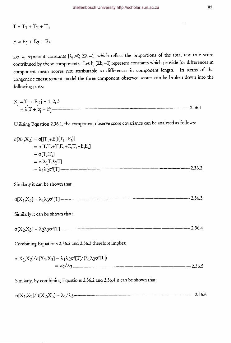
85
Let Ai represent constants [\ >0; L.Ai = 1] which reflect the proportions of the total test true score
contributed by the w components. Let bi [L.bi =0] represent constants which provide for differences in
component mean scores not attributable to differences in component length. In terms of the
congeneric measurement model the three component observed scores can be broken down into the
following parts:
Xj = Tj + Ej; j = 1, 2, 3
= AjT + bj + Ej -------------------------------------------------------------- 2.36.1
Utilising Equation 2.36.1, the component observe score covariance can be analysed as follows:
cr[X1,X2J = cr[(f1+E1)(f2 +EJ]
= cr[T1T 2+ T 1E2 +E1T 2 +E1E2]
= cr[Tt,Tz]
= cr[A1T,A2T]
= A 1 A zcr2[T] --------------------------------------------------------------------------------- 2.3 6.2
Similarly it can be shown that:
cr[X 1 ,X 3] = A 1 A 3 cr2[T] ------------------------------------------------------------------------------------ 2. 3 6. 3
Similarly it can be shown that:
cr[X 2,X 3] = A 2 A 3 cr2[T] -------------------------------------------------------------------------------- 2. 3 6. 4
Combining Equations 2.36.2 and 2.36.3 therefore implies:
cr[X 1,X2]/ cr[X 1,X 3] = A1 A2cr2[T]/ (A1 A 3cr2[T])
= A21A 3 -------------------------------------------------------- 2.36.5
Similarly, by combining Equations 2.36.2 and 2.36.4 it can be shown that:
cr[X 1 ,X 2J/ cr[X 2,X 3] = A 1 I A 3---------------------------------------------------------------------------------- 2. 3 6. 6
Stellenbosch University http://scholar.sun.ac.za
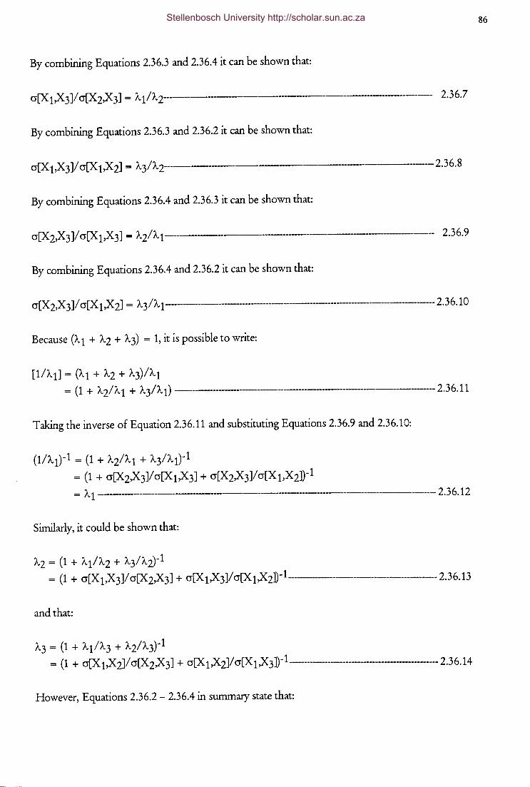
86
By combining Equations 2.36.3 and 2.36.4 it can be shown that:
cr[X 1 ,X 3]/ cr[X 2,XJ] = A 1 /A 2--------------------------------------------------------- 2.36.7
By combining Equations 2.36.3 and 2.36.2 it can be shown that:
By combining Equations 2.36.4 and 2.36.3 it can be shown that:
cr[X2,X3]/cr[X1,X3] = A2/A1--------------------------------- ------------ 2.36.9
By combining Equations 2.36.4 and 2.36.2 it can be shown that:
cr[X 2,X 3 ]/ cr[X 1 ,X 2J = A 3 I A 1------------------------------------------------------------------------------------- 2. 3 6.10
Because (A1 + A2 + A3) = 1, it is possible to write:
[1/A1] = (A1 + A2 + A3)/A1 = ( 1 + A 2/ A 1 + A 3/ A 1) ------------------------------------------------------------------------ 2.3 6.11
Taking the inverse of Equation 2.36.11 and substituting Equations 2.36.9 and 2.36.10:
(1/A1)-1 = (1 + A2/A1 + A3/A1)-1
= (1 + cr[X2,X3]/cr[X1,X3] + cr[X2,X3]/cr[XbX2])-1
= A 1 ------------------------------------------------------------------------------------------- 2. 3 6.12
Similarly, it could be shown that:
A2 = (1 + A1/A2 + A3/A2)-1 = ( 1 + cr[X 1 ,X 3]/ cr[X 2X 3] + cr[X 1 ,X 3]/ cr[X 1 ,X 2])-!_ _____________________________________ 2.3 6.13
and that:
A3 = (1 + A1/A3 + A2/A3)-1 = (1 + cr[X 1,X2]/ cr[X2,X3] + cr[X 1X2J/ cr[X 1X3])-L-------------------------------------------- 2.36.14
However, Equations 2.36.2 - 2.36.4 in summary state that:
Stellenbosch University http://scholar.sun.ac.za
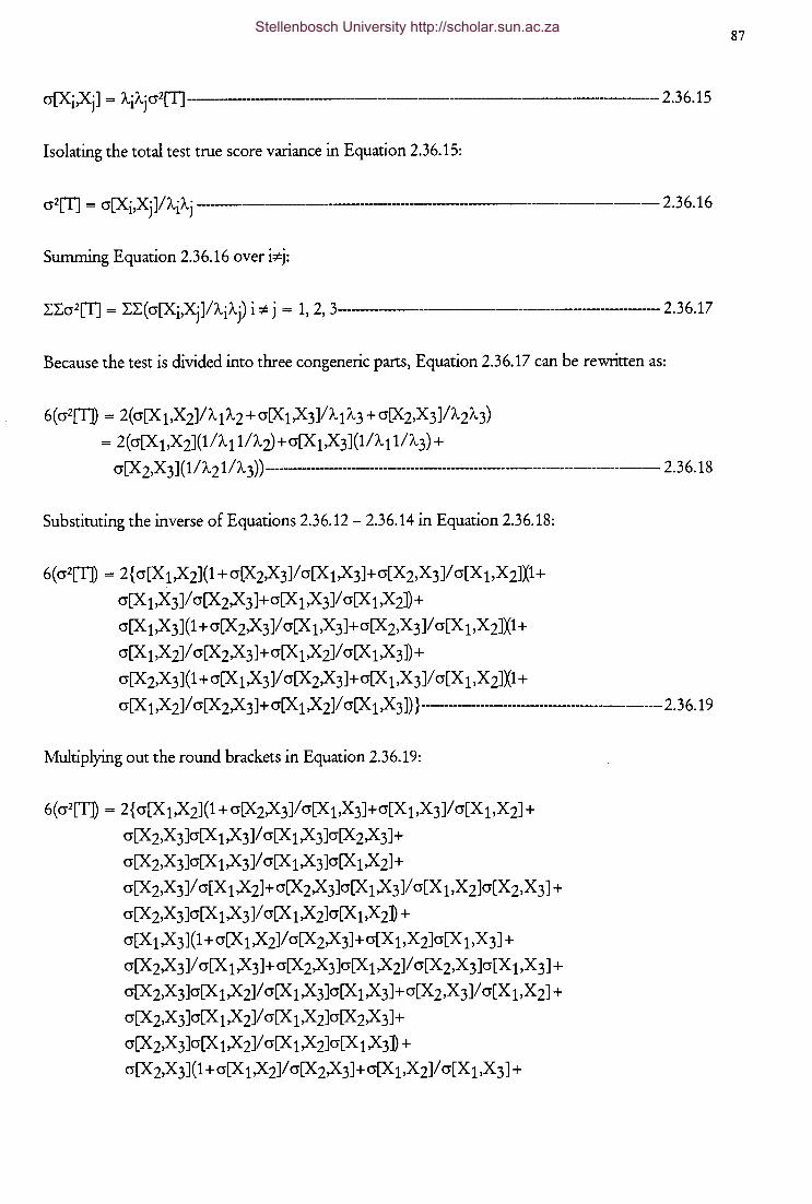
cr[Xi,Xj] = /..iAjcr2[TJ-------------------·--- ---- 2.36.15
Isolating the total test true score variance in Equation 2.36.15:
·------------ ·-------------------- 2.36.16
Summing Equation 2.36.16 over i:;e:j:
LLcr2[T] = LL(cr[Xi,Xj]IAiAj) i :;e: j = 1, 2, 3-------------------------------------------2.36.17
Because the test is divided into three congeneric parts, Equation 2.36.17 can be rewritten as:
6(cr2[T]) = 2(cr[X 1,X2]IA1 A2 +cr[X1,X3]IA1 A3 +cr[X2,X3]IA2A3)
= 2(cr[X 1,X2](11A111A2)+cr[X 1,X3](1IA11IA3) +
cr[X 2,X 3] ( 1 I A 21 I A 3)) --------------------------------------------------------------------------- 2. 3 6.18
Substituting the inverse of Equations 2.36.12 - 2.36.14 in Equation 2.36.18:
6(cr2[T]) = 2{ cr[X 1X2](1 + cr[X2,X3]I cr[X 1,X3]+cr[X2,X 3]l cr[X 1,X2JX1 +
cr[X 1,X3]I cr[X2,X3]+cr[X 1X3JI cr[X 1X2J)+
cr[X 1,X3](1 +cr[X2,X3]I cr[X 1,X3]+cr[X2,X 3]l cr[X 1,X2JX1 +
cr[X 1,X2JI cr[X2,X3]+cr[X 1X2JI cr[X 1,X3])+
cr[X2,X3](1 +cr[X 1X3JI cr[X2,X3]+cr[X 1,X 3]l cr[X 1,X2JX1 +
cr[X 1 ,X 2JI cr[X 2X 3]+ cr[X 1 ,X 2JI cr[X 1 X 3])} ------------------------------------------- 2. 3 6.19
Multiplying out the round brackets in Equation 2.36.19:
6(cr2[T]) = 2{cr[X 1,X2](1 +cr[X2,X3]Icr[X 1,X3]+cr[X 1,X3]Icr[X 1,X2J+
cr[X2,X3]cr[X 1,X3]I cr[X 1,X3]cr[X2,X3]+
cr[X2,X3]cr[X 1,X3]Icr[X 1,X3]cr[X 1X2J+
cr[X2,X3]I cr[X 1X2J+cr[X2,X3]cr[X 1,X3]I cr[X bX2]cr[X2,X 3] +
cr[X2,X3]cr[X 1X3JI cr[X 1X2Jcr[X 1X2] +
cr[X 1,X3](1 +cr[X 1X2JI cr[X2,X3]+cr[X 1,X2]cr[X 1,X 3]+
cr[X2,X3]I cr[X 1,X3]+cr[X2,X3]cr[X 1X2JI cr[X2,X 3]cr[X 1,X3] +
cr[X2,X3]cr[X 1X2JI cr[X 1,X3]cr[X 1,X3]+cr[X2,X 3]l cr[X 1,X2J +
cr[X 2,X 3]cr[X 1 ,X 2JI cr[X 1 ,X 2Jcr[X 2X 3]+
cr[X 2,X 3]cr[X 1 ,X 2JI cr[X 1 ,X 2Jcr[X 1 X 3] +
cr[X2,X3](1 +cr[X 1X2JI cr[X2,X3]+cr[X 1,X2JI cr[X 1,X 3] +
87 Stellenbosch University http://scholar.sun.ac.za
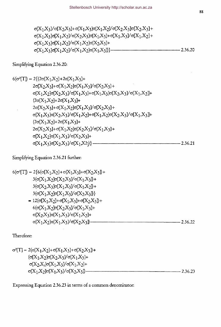
cr[X 1,X3]/ cr[X2,X3]+cr[X 1X3]cr[X 1X2J/ cr[X2,X 3]cr[X2,X 3] +
cr[X 1,X 3]cr[X 1X2J/ cr[X2,X 3]cr[X 1X 3]+cr[X 1,X 3]/ cr[X 1,X2J +
cr[X 1X3]cr[X 1X2J/ cr[X 1X2Jcr[X2,X3]+
cr[X 1X 3]cr[X 1X2J/ cr[X 1X2Jcr[X 1X3]} ----·--
Simplifying Equation 2.36.20:
6(cr2[T]) = 2{(2cr[X1,X2]+2cr[X1,X3]+
2cr[X2,X3]+cr[X 1X2Jcr[X 1X3J/ cr[X2,X3] +
cr[X 1,X2]cr[X2,X3]/ cr[X 1X3J+cr[X 1X3]cr[X2,X3]/ cr[X 1,X2J}t
(2cr[X 1X2J+ 2cr[X 1X 3]+
2cr[X 2,X 3]+ cr[X 1 ,X 2]cr[X 1 ,X 3]/ cr[X 2X 3] +
cr[X 1,X3]cr[X2,X3]/cr[X 1X2J+cr[X 1X2]cr[X2,X 3]/ cr[X 1,X 3])t
(2cr[X 1,X2]+2cr[X 1X3]+
2cr[X2,X3]+cr[X 1X2Jcr[X2,X3]/ cr[X 1X3J+
cr[X 1X2Jcr[X 1,X 3]/ cr[X2,X3]+
2.36.20
cr[X 1 ,X 3]cr[X 2,X 3]/ cr[X 1 X2J)} ------------------------------------------------ 2.3 6.21
Simplifying Equation 2.36.21 further:
6(cr2[T]) = 2{ 6(cr[X 1,X2J+cr[X1,X3]+cr[X2,X3])+
3(cr[X 1,X2]cr[X2,X3]/ cr[X 1X3J)+
3 ( cr[X 2,X 3]cr[X 1 ,X 3]/ cr[X 1 ,X 2]) +
3(cr[X 1,X2]cr[X 1X3]/ cr[X2,X3]}
= 12(cr[X 1,X2J+cr[X 1X3]+cr[X2,X3])+
6( cr[X 1,X2]cr[X2,X3]/ cr[X 1X 3]+
cr[X2,X 3]cr[X 1,X 3]/ cr[X 1X2J+
cr[X 1 ,X 2Jcr[X 1 ,X 3 ]/ cr[X 2X 3]) ------------------------------------------------------------------ 2.3 6.22
Therefore:
cr2[T] = 2(cr[X 1,X2J+cr[X 1,X3]+cr[X2,X3])+
(cr[X 1,X2]cr[X2,X 3]/ cr[X 1X3J+
cr[X2,X3]cr[X 1X3]/ cr[X 1X2J+
cr[X 1 ,X 2Jcr[X 1 ,X 3 ]/ cr[X 2X 3] ---------------------------------------------------------- 2. 3 6.23
Expressing Equation 2.36.23 in terms of a common denominator:
88 Stellenbosch University http://scholar.sun.ac.za
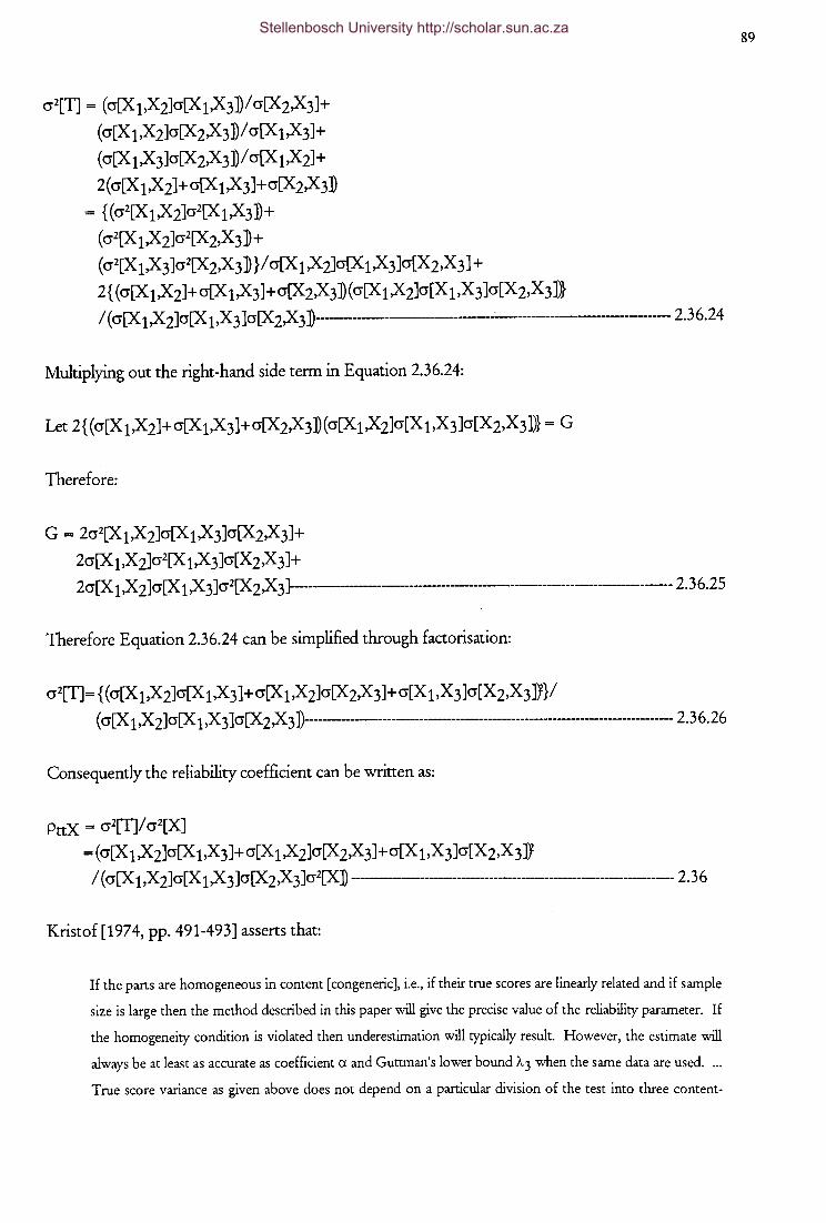
cr2[T] = (cr[X1,X2]cr[X1,X3])Icr[X2,X3]+
(cr[X 1,X2]cr[X2,X3]I cr[X 1X3]+
(cr[X 1X3]cr[X2,X3])I cr[X 1X2J+
2(cr[X 1,X2J+cr[X 1X3]+cr[X2,X3]
= {(cr2CX1X2Jcr2[X1,X3]+
(cr2[X 1,X2]cr2[X2,X 3]+
(cr2[X 1,X 3]cr2[X2,X 3] }I cr[X 1X2Jcr[X 1X3]cr[X2,X 3] +
2{ (cr[X 1X2J+cr[X 1X3]+cr[X2,X3])(cr[X 1X2Jcr[X 1,X 3]cr[X2,X 3])}
I ( cr[X 1X2]cr[X 1,X 3]cr[X2,X 3])------------------__:..------------------- 2.36.24
Multiplying out the right-hand side term in Equation 2.36.24:
Therefore:
G = 2cr2[X 1X2Jcr[X 1X3]cr[X2,X3]+
2cr[X 1,X 2]cr2[X 1,X 3]cr[X2,X 3]+ 2cr[X 1 ,X 2Jcr[X 1 ,X 3]cr2[X 2X 3}----------------------------------------------------------------- 2.3 6.25
Therefore Equation 2.36.24 can be simplified through factorisation:
cr2[T]= { (cr[X 1,X2]cr[X 1,X3]+cr[X 1,X2]cr[X2,X3]+cr[X bX 3]cr[X2,X 3]}}l
( cr[X 1 ,X 2Jcr[X 1 ,X 3 ]cr[X 2X 3])-------------------------------------------------------------------------- 2. 3 6. 26
Consequently the reliability coefficient can be written as:
PttX = cr2[TJI cr2[X]
=(cr[X 1X2Jcr[X 1,X3]+cr[X 1X2]cr[X2,X3]+cr[X 1,X 3]cr[X2,X 3]}
I ( cr[X 1 ,X 2Jcr[X 1 ,X 3 ]cr[X 2X 3]cr2[X]) -------------------------------------------------------- 2. 3 6
Kristof [1974, pp. 491-493] asserts that:
If the parts are homogeneous in content [congeneric], i.e., if their true scores are linearly related and if sample
size is large then the method described in this paper will give the precise value of the reliability parameter. If
the homogeneity condition is violated then underestimation will typically result. However, the estimate will
always be at least as accurate as coefficient a and Guttman's lower bound A.3 when the same data are used ....
True score variance as given above does not depend on a particular division of the test into three content-
89 Stellenbosch University http://scholar.sun.ac.za
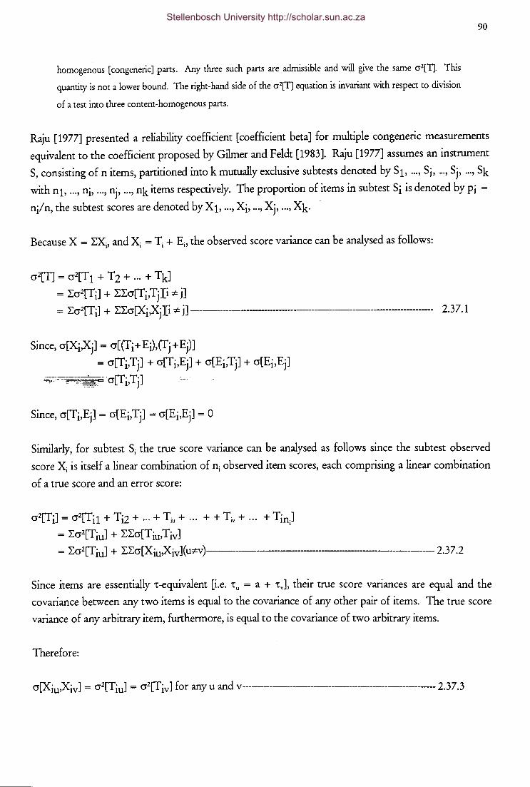
homogenous [congeneric] parts. Any three such parts are admissible and will give the same cr2[T]. This
quantity is not a lower bound. The right-hand side of the cr2[T] equation is invariant with respect to division
of a test into three content-homogenous parts.
90
Raju [1977] presented a reliability coefficient [coefficient beta] for multiple congeneric measurements
equivalent to the coefficient proposed by Gilmer and Feldt [1983]. Raju [1977] assumes an instrument
S, consisting of n items, partitioned into k mutually exclusive subtests denoted by S1, ... , Si, -·• Sj, ... , Sk
with n 1· ... , ni, ... , nj, ... , nk items respectively. The proportion of items in subtest Si is denoted by Pi =
n/n, the subtest scores are denoted by X 1• ... ,Xi, ... , Xj, ... , Xk -
Because X = L~, and~ = Ti + Ei, the observed score variance can be analysed as follows:
cr2[TJ = cr2[T1 + T2 + ... + Tk]
= Lcr2[Ti] + LLcr[Ti,Tj][i * j] = Lcr2[T iJ + LLcr[Xi,Xj][i "* j] -------------------------------------------------------------------------- 2. 3 7.1
Since, cr[Xi,Xj] = cr[(fi+EJ,(fj+Ej)J
= cr[Ti,Tj] + cr[Ti,Ej] + cr[Ei,Tj] + cr[Ei,Ej]
· ~"-~-~-:--~-~;::c.:: cr[Ti,Tj]
Similarly, for subtest Si the true score variance can be analysed as follows since the subtest observed
score Xi is itself a linear combination of ni observed item scores, each comprising a linear combination
of a true score and an error score:
cr2[Ti] = cr2[Ti1 + Ti2 + ··· + Tiu + ··· + + Tiv + ··· + Tin.J 1
= Lcr2[TiuJ + LLcr[TiwTivJ
= Lcr2[T iuJ + LLcr[XiuXiv] ( u;f:;v)-------------------------------------------------------- 2. 3 7.2
Since items are essentially -c-equivalent [i.e. -cu = a + 'tJ, their true score variances are equal and the
covariance between any two items is equal to the covariance of any other pair of items. The true score
variance of any arbitrary item, furthermore, is equal to the covariance of two arbitrary items.
Therefore:
cr[XiwXivJ = cr2[TiuJ = cr2[TivJ for any u and v------------------------------------------------------------- 2.37.3
Stellenbosch University http://scholar.sun.ac.za

Let g represent cr2[TiuJ
Equation 2.37.2 can therefore be rewritten as:
cr2[TJ = nig + ni(ni- l)g
= nig + ni2g - nig
= n?g-- ·-------------------------------------------------- 2.37.4
Using Equation 2.37.4, Equation 2.27.1 can be rewritten as:
cr2[T] = Ln?g + LLcr[Xi,Xj]
= gLn? + LLcr[Xi,Xj] ------------------------------------------------------------------ 2.3 7.5
However:
Therefore:
cr[Xi,Xj] = gninj ----------------------------------------------------------------------------------------------------------- 2.3 7. 6
Therefore:
L Lcr[Xi,X j] = gLLni n j -------------------------------------------------------------------------------------------------- 2. 3 7. 7
Isolating gin Equation 2.37.7 results in:
g = LLcr[Xi,Xj]/LLninj ----------------------------------------------------------------------------- 2. 3 7. 8
91
Substituting Equation 2.37.8 into Equation 2.37.5 and multiplying the covariance term with
LLnin/LLninj results in:
cr2[T] = gLni2 + LLcr[Xi,Xj]
= { (Lni2LLcr[Xi,Xj])/LLninj} + LLcr[Xi.XjJ
= { (Ln?LLcr[Xi,Xj])/LLninj} + (LLninjLLcr[Xi,Xj]J'LLninj
= LLcr[Xi,Xj]{ (Ln? + LLn in j)/LLn i nj} -------------------------------------------------------------- 2. 3 7. 9
Stellenbosch University http://scholar.sun.ac.za
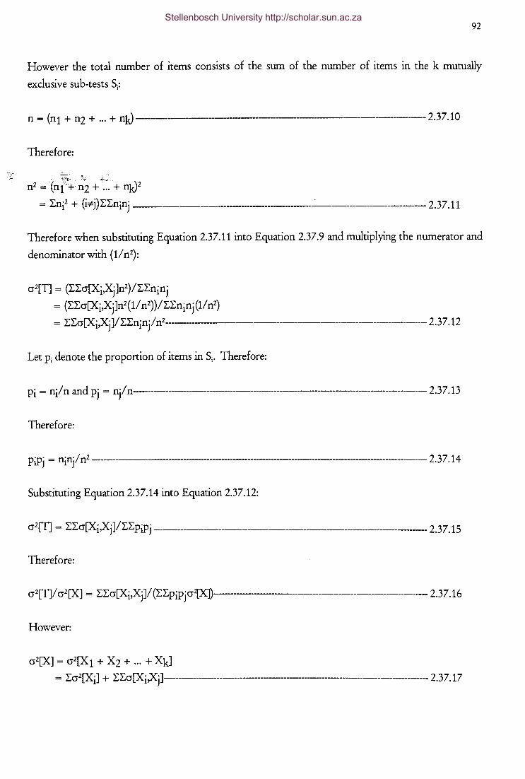
92
However the total number of items consists of the sum of the number of items in the k mutually
exclusive sub-tests Si:
n = (n1 + n2 + ... + nk)-----·---· ---------------------------- 2.37.10
Therefore:
-:?.~~-- ;.~-n2 = '(nf"+ n2 + ... + nk)2
= I:n? + (i:t:j)I:I:ninj ______________________________ _:_ ___________________________ 2.37.11
Therefore when substituting Equation 2.37.11 into Equation 2.37.9 and multiplying the numerator and
denominator with ( 11 n2):
cr2[T] = (I:I:cr[Xi,Xj]n2)/I:I:ninj
= (I:I:cr[Xi,Xj]n2(1/ n2))/I:I:ninj (1/ n2)
= I:I:cr[XiXjJ/I:I:ni njl n2----------------------------------------------------------------------- 2.3 7.12
Let Pi denote the proportion of items in Si. Therefore:
Pi = ni/ n and Pj = njl n----------------------------------------------------------------------------------------------- 2.37.13
Therefore:
P~j=~~~~---------------------------------------------------2.3~14
Substituting Equation 2.37.14 into Equation 2.37.12:
cr2[T] = I:I:cr[Xi,Xj]/I:I: P~j ---------------------------------------------------------------------- 2. 3 7.15
Therefore:
cr2[T]/ cr2[X] = I:I:cr[Xi,Xj]/ (I:I:pipjcr{X])--------------------------------------------------------- 2.37.16
However:
cr2[XJ = cr2[X1 + X2 + ... + Xk]
= I:cr2[Xi] + I:I:cr[Xi.XjJ--------------------------------------------------------------------------------- 2.3 7.17
Stellenbosch University http://scholar.sun.ac.za
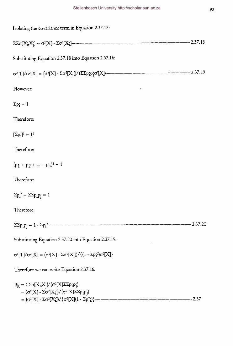
93
Isolating the covariance term in Equation 2.37.17:
I:I:cr[Xi,Xj] = cr2[X] - I:cr2[XiJ-------------------------------------------------------------------------- 2.3 7.18
Substituting Equation 2.37.18 into Equation 2.37.16:
cr2['n/ cr2[X] = ( cr2[X] - I:cr2[Xi] I (I: I: piP j cr2(X])------------------------------------------- 2.3 7.19
However:
Therefore:
Therefore:
(p1 + P2 + ··· + PlJ2 = 1
Therefore:
Therefore:
2:2: PiP j = 1 - 2: pi 2 -------------------------------------------------------------------------------------------------------- 2. 3 7. 2 0
Substituting Equation 2.37.20 into Equation 2.37.19:
Therefore we can write Equation 2.37.16:
~k = I:I:cr[Xi,Xj]/(cr2[X]I:I:pipj)
= (cr2[X]- I:cr2[Xi])/(cr2[X]I:I:pipj)
= (cr2[X] - I:cr2[Xi])/ { cr2[X](1 - I:p2J} ------------------------------------------------------------------------2.37
Stellenbosch University http://scholar.sun.ac.za
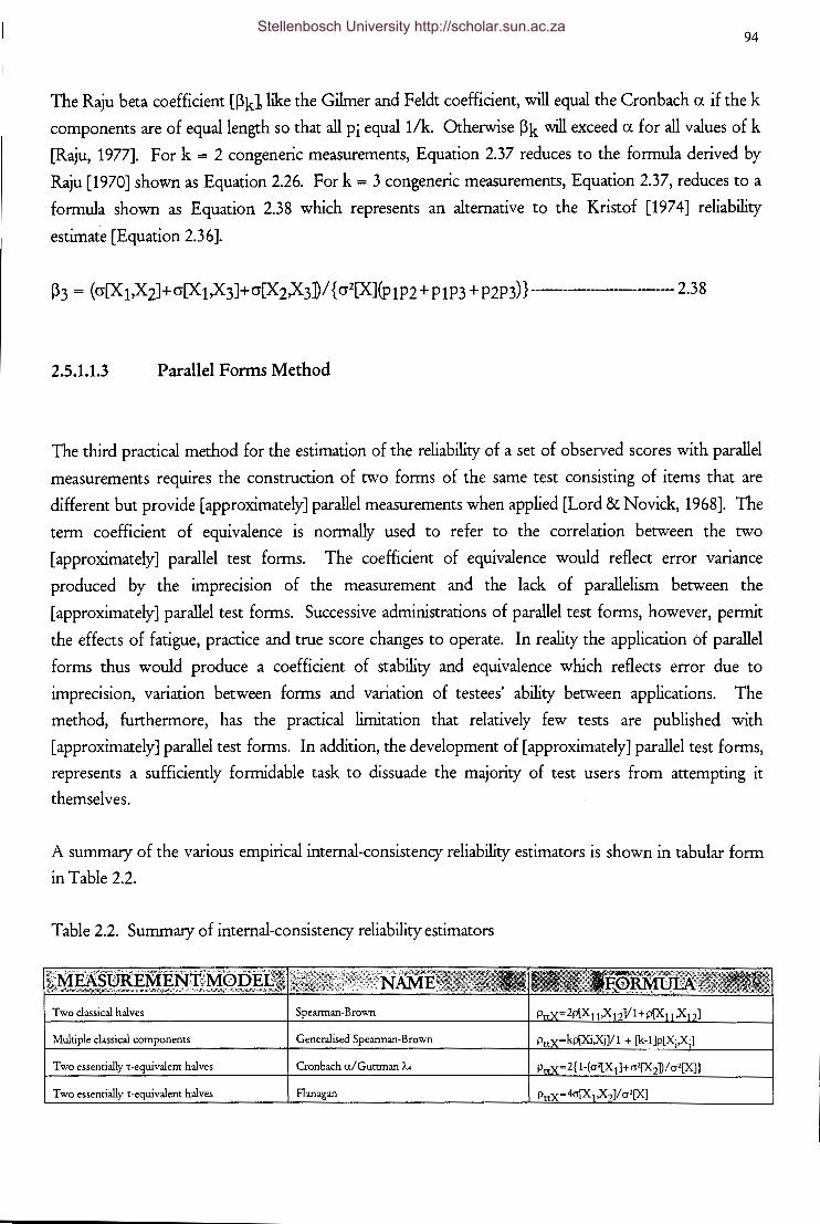
94
The Raju beta coefficient Wk1like the Gilmer and Feldt coefficient, will equal the Cronbach a if the k
components are of equal length so that all Pi equal 1/k. Otherwise Pk "'Will exceed a for all values of k
[Raju, 1977]. Fork= 2 congeneric measurements, Equation 2.37 reduces to the formula derived by
Raju [1970] shown as Equation 2.26. Fork= 3 congeneric measurements, Equation 2.37, reduces to a
formula shown as Equation 2.38 which represents an alternative to the Kristof [197 4] reliability
estimate [Equation 2.36].
2.5.1.1.3 Parallel Forms Method
The third practical method for the estimation of the reliability of a set of observed scores with parallel
measurements requires the construction of two forms of the same test consisting of items that are
different but provide [approximately] parallel measurements when applied [Lord & Novick, 1968]. The
term coefficient of equivalence is normally used to refer to the correlation between the two
[approximately] parallel test forms. The coefficient of equivalence would reflect error variance
produced by the imprecision of the measurement and the lack of parallelism between the
[approximately] parallel test forms. Successive administrations of parallel test forms, however, permit
the effects of fatigue, practice and true score changes to operate. In reality the application of parallel
forms thus would produce a coefficient of stability and equivalence which reflects error due to
imprecision, variation between forms and variation of testees' ability between applications. The
method, furthermore, has the practical limitation that relatively few tests are published with
[approximately] parallel test forms. In addition, the development of [approximately] parallel test forms,
represents a sufficiently formidable task to dissuade the majority of test users from attempting it
themselves.
A summary of the various empirical internal-consistency reliability estimators is shown in tabular form
in Table 2.2.
Table 2.2. Summary of internal-consistency reliability estimators
Two classical halves
Multiple classical components
Two essentially <-equivalent halves Cronbach a/Gunman A.
Two essentially 't-emuvale:nt halves Flanagan
-------------------------------------------------~
Stellenbosch University http://scholar.sun.ac.za

95
Two essentially t-equivalent halves Rulon PttX=1- a2[X1-X2Va'[X]
Two classical halves Rulon Pnx=1- {a'[Xt-Ya'[X]}
Two congeneric halves Raju pttX-a[X1,XzVt..tt..za'[X]
Two congeneric halves Feldt pttX= 4a[X 1 X 2V { a2(X] -[(a2[X1] -
a2[X 2:01 a[X]J2}
Essentially t-equivalent components Cronbacha a=[k/(k-1)11- I:a2£XiVa2(X]]
Essentially t -equivalent components Kuder-Richardson-20 pttX=[k/(k-1)11- I:P·Q·/a2(X]]
Essentially t-equivalent components Kuder-Richardson-21 pttX=[k/(k-1)11-kJ.l[PMQVaW
Essentially t-equivalent components Guttman/..2 t..2=[II:a(XjXjl+ {kl(k-
1)Lra2DCj,X·]} 'h]/a2(X]
Multiple congeneric Gilmer & Feldt pttX= { 11 ( 1-L/..•2)} { 1-I:a2£Xi]l a2(X]}
Multiple congeneric Kristof PttX= { a[X1Xzla[X1,X3J+a[X1,Xz]a[XzX3J+
a[X1,X3]a[Xz,X3]}2/a[X1,X2]a[X1,X3]a[Xz,X
3]a2(X]
Multiple congeneric Raju ~k ~k= {a2[X]-I:a2DCjl}/ {a2[X](l-I:p'J}
2.5.2 Validity
Validity is a concept of fundamental importance to psychological measurement. Validity is, however,
also a concept of considerable complexity. Despite this, various niive/limited, if not erroneous,
conceptions of validity have developed to detrimentally effect the debate on personnel decisions based
on psychological measurements [Binning & Barrett, 1989; Schmitt & Landy, 1993]. This tendency
seems to apply especially to human resource practitioners in South Africa.
The theoretical conceptualisation of validity has evolved over the years [Landy, 1986; Messick, 1989,
Schmitt & Landy, 1993], shaped by the combined influence of changing legal, social, economic and
technical considerations on the quality of psychological measurement. Since at least the early 1950's,
test validity has been broken into three distinct types, one of which comprises two subtypes [Messick,
1989]. These are the familiar trinity of content validity, criterion related validity [subsuming predictive
and concurrent validity] and construct validity [Ellis & Blustein, 1991; Landy, 1986; Messick, 1989,
Schmitt & Landy, 1993; Schuler & Guldin, 1991]. The taxonomy itself is not fundamentally flawed
[Landy, 1986] in as far as it suggests that different inferences can be made from test scores. The linkage
of these validity concepts to specific aims of testing by the American Psychological Association in their
technical recommendations on psychological testing [APA, 1954; APA, 1966; APA, 1974], in
conjunction with Title VII litigation case law [Landy, 1986], did however create the erroneous
trinitarian notion that only a single validation type or strategy need to be considered in any given
_ _j
Stellenbosch University http://scholar.sun.ac.za
96
s1tuat10n. Although each subsequent revised edition of the Standards for educational and psychological
tests/ testing did to a certain, albeit diminishing, degree perpetuate this erroneous distinction between
validity types, they did, however, gradually move towards a unificationist perspective on the validity
concept [Messick, 1989].
A central thesis developed in chapter 1 is that measurements are obtained by reason of the need for
quantitative information on constructs for the purpose of decision-making. The relevance of
information on a construct for a particular decision is, in the final analysis, based on logical and ethical
considerations rather than empirical psychometric evidence. The question, which constructs to obtain
information on, therefore, is not a psychometric question.
Due to the abstract nature of psychological constructs, information on their states or levels can be
inferred only from their observable effects. The question consequently arises to what extent the
operationalisation of the relevant construct in terms of observable denotations was successful. The
pivotal question is to what extent the measurement procedure produces a pure [i.e. uncontaminated by
irrelevant influences] and comprehensive [i.e. complete coverage of all facets of the construct as
constitutively defined] quantitative description of the [multi-dimensional] construct regarded as relevant
for the decision at hand. An alternative, more prevalent formulation of the above interpretation would
be to define validity as the degree to which an instrument measures the construct which it claims or
intends to measure [Nunnally, 1978]. Validity thus refers to the degree to which variance in a set of
measures is due to variance in the underlying construct of interest [Guion, 1965]. The validity of a set
of measurements refers to the formal consideration of the preceding question. If all personnel
decisions could be made in terms of quantitative descriptions of constructs measurable at the time of
the decision, the foregoing basic conceptualisation of validity would probably have sufficed. This is,
however, not the case. For an important class of personnel decisions information on the construct
deemed relevant to the decision cannot be obtained prior to the decision.
To provide for this eventuality, while still remaining relevant to the earlier discussion, validity can more
generally be interpreted as the extent to which the inferences made from the test scores are in fact
warranted; the extent to which the interpretation [i.e. meaning] assigned to test scores is
justified/ supported. Strictly speaking, therefore, what is being validated is not the measuring
instrument, nor the measures obtained from the instrument, but rather the inferences made from the
measures'. Messick [1989, p. 13], in his monumental and definitive treatment of the validity concept,
states:
1 The same principle also applies for any other context in which the validity concept is used; research designs, for example, can be designated internally valid to the extent that they permit causal inferences of the form Y=f[X].
Stellenbosch University http://scholar.sun.ac.za
Validity is an integrated evaluative judgement of the degree to which empirical evidence and theoretical
rationales support the adequacy and appropriateness of inferences and actions based on test scores or other
modes of assessment. .... Broadly speaking, then, validity is an inductive summary of both the existing
evidence for and the potential consequences of score interpretation and use. Hence what is to be validated is
not the device as such but the inferences derived from test scores or other indicators - inferences about score
meaning or interpretation and about the implications for action that the interpretation entails.
97
Validation, in turn, refers to the process of accumulating and cementing empirical evidence and logical
thought in a credible argument in defense of the inferences made from the observed scores. Kane
[1992, p. 527] expresses his views on an argument-based approach to validation as follows:
A test-score interpretation always involves an interpretive argument ..... To validate a test-score interpretation
is to support the plausibility of the corresponding interpretive argument with appropriate evidence. The
argument-based approach to validation adopts the interpretive argument as the framework for collecting and
presenting validity evidence and seeks to provide convincing evidence for its inferences and assumptions,
especially its most questionable assumptions.
The type of validity evidence required to justify the inferences made from test scores depends on the
nature of the interpretive argument. This 1-hould, however, not be construed to mean that a single
validity analysis strategy [Lawsche, 1985] should be chosen from the trilogy of content, construct and
criterion-related validities [Ellis & Blustein, 1991; Landy, 1986 ]. The different validity analysis strategies
are not alternatives but rather form supplementary facets of a single unitary validity concept [Binning &
Barrett, 1992; Ellis & Blustein, 1991; Guion, 1991; Messick, 1989; Schmitt & Landy, 1993]. Schmitt
and Landy [1993, p. 286] clearly affirm the foregoing position by stating:
Marshaling evidence of validity is now seen as a process of theory development and testing [Binning &
Barrett, 1989; Landy, 1986]. We must develop and articulate theories of job performance and define logically
the constructs that are central to these theories. We must establish a 'nomological network' that relates
constructs important in the job performance domain to the constructs we choose to identify qualified job
applicants. This requires evidence that the measures we use to operationalize constructs in the predictor and
performance domains possess a logical relationship to these constructs and empirically consistent
relationships to other measures of the construct.
The recognition of the inappropriateness of using the trinitarian conceptualisation of validity in a way
that resembles "stamp collecting" [Landy, 1986], in essence rests on the realisation that personnel
selection decisions are not based on a single inference but rather an integrated network of inferences or
a multi-step argument. In personnel selection decisions, job performance forms the basis [i.e., the
criterion] on which applicants should be evaluated so as to determine their assignment to an
Stellenbosch University http://scholar.sun.ac.za
98
appropriate treatment [Cronbach, 1965]. Information on actual job performance can, however, never
be available at the time of the selection decision. This seemingly innocent, but too often ignored,
dilemma provides the impetus for the development of the aforementioned integrated network of
inferences or multi-step argument. Even though it is logically impossible to obtain direct information
on the performance construct [i.e., the final/ultimate criterion] at the time of the selection decision, it
can nonetheless be predicted at the time of the selection decision if:
);> variance in the performance construct can be explained in terms of one or more
predictors;
);> the nature of the relationship between these predictors and the performance
construct has been made explicit; and
);> predictor information can be obtained prior to the selection decision.
The point of departure for the development of any personnel selection procedure is the performance
construct [Binning & Barrett, 1989]. Job analysis provides the necessary information on the job
content and context to constitutively define the performance construct. Two qualitatively different
arguments exist in terms of which predictors can be derived from the conceptualisation of job
performance. Binning and Barrett (1989] seem to be of the same opinion. Although they initially refer
to "three routes from the performance domain to predictor development" they later propose that "the
construct-related and content-related approaches represent the two fundamental predictor sampling
strategies""[Binning & Barrett, 1989, p. 483]. This position, previously described in chapter 1,
correlates with a distinction Wernimont and Campbell [1968] makes between predictors as signs and
predictors as samples. Since these two different approaches to predictor development rely on
quantitatively different arguments they have to be justified in terms of different types of validity
evidence.
A construct-related approach to predictor development utilises the conceptualisation of the
performance construct in conjunction with theory and logic to develop through theorising a complex
performance hypothesis [a tentative nomological network] as a tentative performance theory. If the
complex performance hypothesis would in fact be valid, it would in principle be possible to estimate
job performance as a substitute for actual job performance [provided the nature of the relationship
between the performance construct and its person-centered determinants would also be known].
Personnel selection procedures are thus possible in terms of this approach only if they are based on a
valid substantive performance hypothesis. The efficiency of such procedures would in turn depend on
to the extent to which the underlying performance hypothesis reflects the full complexity of the forces
shaping job performance [both in terms of the nature of the determinants and the way they combine].
To establish the validity of the performance hypothesis, an operational hypothesis is deductively
derived from the substantive performance hypothesis by operationally defining the performance
construct and the explanatory psychological constructs. The operational definition of the performance
Stellenbosch University http://scholar.sun.ac.za

99
construct constitutes a premise in the aforementioned deductive argument, as do the operational
definitions of the explanatoty psychological constructs. The validity of the deductive argument
depends on the validity of these premises [Copi & Cohen, 1990; Mouton & Marais, 1985]. In a valid
deductive argument the premises provide conclusive grounds for the truth of the conclusion [Copi &
Cohen, 1990]. The justifiability of the claim that the operational performance hypothesis constitutes a
valid testable representation of the theoretical performance hypothesis thus depends on the construct
validity of the operational measures of the performance construct and the explanatory psychological
determinants. Should empirical confirmation for the operational performance hypothesis be found
[assuming that the aforementioned deductive argument was in fact valid], the substantive performance
hypothesis may be considered corroborated since it has survived an opportunity to be refuted [Popper,
1972]. The validity of the substantive performance hypothesis, in conjunction with evidence on the
construct validity of the operational measures of the explanatory psychological constructs, provides
justification for the claim that job performance can be inferred from an array of operational predictor
measures developed through a construct-related approach. Binning and Barrett [1989] consequently
propose five inferences or hypotheses to be central to the validation of a personnel selection procedure,
namely:
~ the [multidimensional] performance/ criterion construct is related to [and thus could
in principle be inferred from] an array of systematically interrelated [possibly also
multidimensional] predictor or person-centered constructs [linkage 1]; and
~ a[n] [multidimensional] operational criterion measure provides a pure and
comprehensive empirical grasp on the [multidimensional] performance construct
[linkage 2] so as to practically enable the inference of the latter from the former; and
~ an array of operational predictor measures provide empirical grasps on the array of
corresponding predictor constructs [linkage 3] so as to practically enable the
inference of the latter from the former; and consequently
~ the operationalised performance/ criterion construct is related to [and thus could be
inferred from] an array of systematically interrelated operationalised predictor or
person-centered constructs[ linkage 4], and consequently
~ the [multidimensional] performance construct is related to [and thus could be
inferred from] an array of systematically interrelated operational predictor or
person-centered measures [linkage 5].
These five pivotal linkages in the interpretive argument [Kane, 1992] or nomological network [Schmitt
& Landy, 1993] underlying selection instrument score interpretation in the context of personnel
selection are depicted in Figure 2.1. In personnel selection research the inference of prime importance
is linkage 5. The critical inference that needs to be justified is therefore the linkage [linkage 5] between
the predictor battery and the theoretical criterion/performance construct [Binning & Barrett, 1989;
Stellenbosch University http://scholar.sun.ac.za
100
Schmitt & Landy, 1993]]. The claim that actual job performance can be inferred from information
obtained from selection techniques, needs to be substantiated.
The criterion-related validity coefficient examines the validity of the hypothesised linkage 4. The
criterion-related validity coefficient, however, only constitutes a necessary, though not sufficient,
element in the evidence required to justify performance inferences from information obtained on the
predictor battery and thus to vindicate a selection procedure should it be challenged in terms of either
efficiency or equity [Milkovich & Boudreau, 1991]. Evidence must also be lead in support of the
hypothesised linkages 2 and 3. The construct validity of the operational predictor and performance
measures must therefore also be established.
A content-related approach to predictor development also utilises the conceptualisation of the
performance construct as the basic point of departure, but now with the purpose of selecting a
representative sample of tasks or demands from the performance domain. A content-related approach
to predictor development requires the development of [low or high fidelity] simulations of the tasks or
demands comprising the performance domain. Inferences regarding future job performance may
justifiably be made from such predictors if sufficient evidence exists that the simulations
comprehensively cover the job performance domain.
Successful performance on the simulation implies successful performance on the job if the demand set
put to the applicant is equivalent to the demand set put to the job incumbent. Therefore, under the
content-related approach to predictor development, the content validity of predictors needs to be
established through empirical and logical analysis. With reference to Figure 2.1, p. 101 the inference of
prime importance is, therefore, still linkage 5. Confidence in linkage 5 can or should, however, be
bolstered by empirically showing that the operational performance measure correlates with the
predictor [i.e., by establishing the criterion-related validity of the predictor or linkage 4]. This in tum,
however, necessitates empirical evidence on the construct validity of the operational
performance/ criterion measure [linkage 2] and the content validity of the predictor measure.
The construct-related and content-related approaches to predictor development clearly differ in terms
of the argument through which they derive selection assessment techniques. It would consequently be
tempting to infer that substantive differences should also exist between construct-related and content
related assessment techniques. This is, however, not the case. Whether the selection technique is a
traditional, construct orientated, psychological test, a low fidelity simulation like a behavioural event
interview, or a high fidelity simulation like virtual reality flying, the essential structure of the
measurement process is the same. A sample of observable behaviour is elicited through a sample of
standardised stimuli under standardised conditions. The elicited behaviour is subsequently observed,
recorded and quantified through a standardised procedure.
Stellenbosch University http://scholar.sun.ac.za
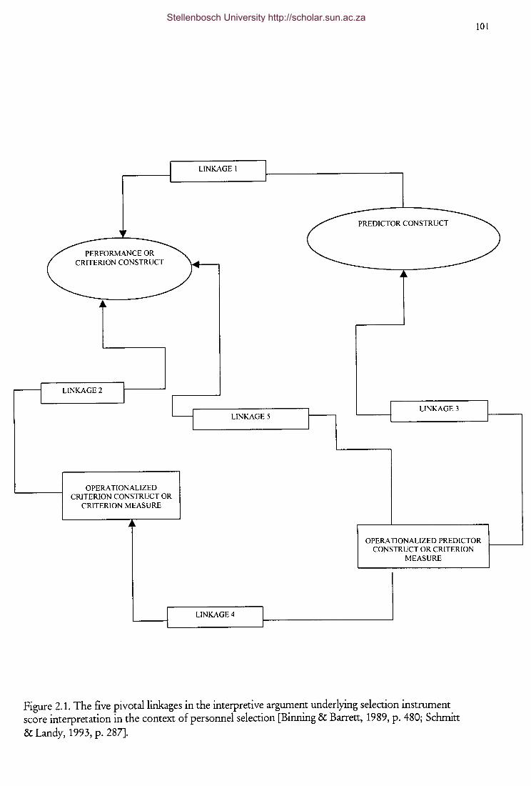
LINKAGE2
OPERA TIONALIZED CRITERION CONSTRUCT OR
CRITERION MEASURE
LINKAGE I
LINKAGE 5
LINKAGE4
101
LINKAGE3
OPERATIONALIZED PREDICTOR CONSTRUCT OR CRITERION
MEASURE
Figure 2.1. The five pivotal linkages in the interpretive argument underlying selection instrument score interpretation in the context of personnel selection [Binning & Barrett, 1989, p. 480; Schmitt & Landy, 1993, p. 287].
Stellenbosch University http://scholar.sun.ac.za
102
The nature and appearance of the [test] stimuli might be different. The logic and processes through
which the stimuli were constructed are necessarily different.
Under a construct-related approach the stimulus sample is constructed so as to reflect, through the
testee's behavioural reaction to it, a specific construct presumed to be relevant to job performance.
Under a content-related approach the stimulus sample is constructed so as to represent the salient job
tasks or demands and thereby to indicate, through the testee's behavioural reaction to it, the applicants
suitability for the job. For a specific job, however, and assuming both types of selection techniques to
have been equally successfully [though differently] justified, the stimulus sample constructed under the
content-related approach would evoke the same psychological constructs than the stimulus sample
constructed under the construct-related approach would. lrrespectiv~ of the approach used to develop
a selection technique, if a selection technique is to have any value at all it must cover the same
psychological constructs that underlie job performance. Under a content-related approach the nature
of the underlying psychological constructs would/ need not be known while the explication of the
nature of the psychological constructs underlying job performance forms the pivot around which the
construct-related approach revolves.
This line of reasoning has additional important implications. Selection techniques developed through a
content-related approach are often perceived to be immune to threats of measurement bias and
decisions based on information obtained from such selection techniques are often seen not to be
susceptible to fairness problems. This seems to be especially true if the selection technique is labeled as
a competency-based approach to assessment. Clearly there exists no psychometric justification for
such beliefs if the essential structure of the measurement process remains the same. In principle the
concepts of bias and fairness apply to assessment techniques derived through a content-related
approach as much as they apply to assessment techniques derived through a construct-related
approach.
From the preceding discussion it is readily apparent that criterion-related validity represents a research
strategy for empirically assessing the quality of both the construct-related and content-related
approaches to predictor development. The criterion-related research strategy, furthermore, constitutes
an indispensable element under both the construct-related and content-related approaches because of
the need to map the operational predictor domain on the operational performance domain. The search
for predictors was initiated because of the unavailability of actual job performance information at the
time of the selection decision and the subsequent need to estimate job performance. All selection
assessments, therefore, need to be interpreted in terms of expected criterion performance [i.e., E[Y I X]]
irrespective of the approach through which the assessment technique was developed. This can only be
achieved if the nature of the relationship between the operationalised performance and predictor
domains are explicitly examined and described.
Stellenbosch University http://scholar.sun.ac.za
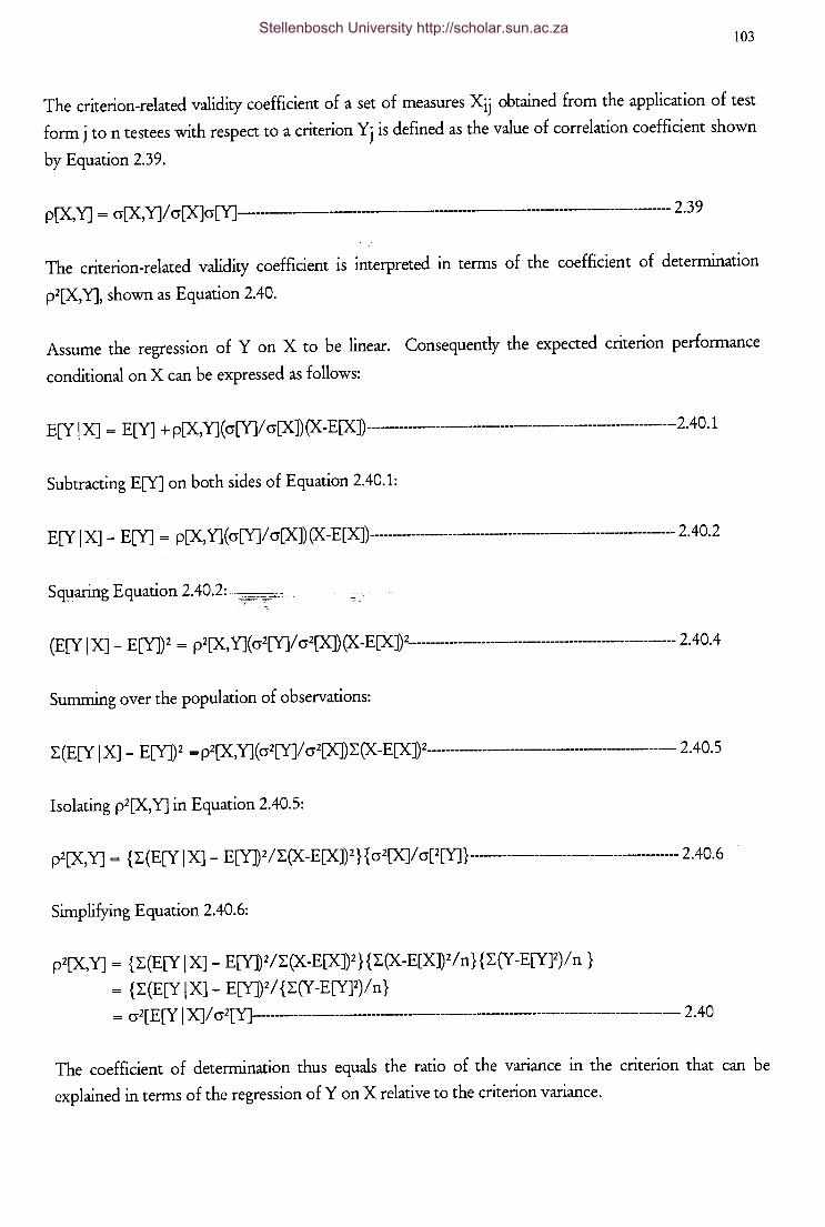
103
The criterion-related validity coefficient of a set of measures Xij obtained from the application of test
form j to n testees with respect to a criterion Yj is defined as the value of correlation coefficient shown
by Equation 2.39.
p[X,Y] = cr[X,Y]/ cr[X]cr[Y]------------------------------------------------------------- 2.39
The criterion-related validity coefficient is interpreted in terms of the coefficient of determination
p2[X,Y], shown as Equation 2.40.
Assume the regression of Y on X to be linear. Consequently the expected criterion performance
conditional on X can be expressed as follows:
E[Y I X] = E[Y] + p[X,Y] ( cr[Y]/ cr[X]) (X-E[X]) -------------------------------------------------------------2.40.1
Subtracting E[Y] on both sides of Equation 2.40.1:
E[Y I X]- E[Y] = p[X,Y](cr[Y]/ cr[X])(X-E[X])----------------------------------------------------------- 2.40.2
Squaring Equation 2.40.2: --~~-c ... - ~T·· ·.~:
(E[Y 1 X] - E[YJ)2 = p2[X, Y]( cr2[Y]/ cr2[X]) (X-E[X])2------------------------------------------------------ 2. 40.4
Summing over the population of observations:
~(E[Y 1 X]- E[YJ)2 =p2[X,Y](cr2[Y]/cr2[X])~(X-E[X])2----------------------------------------- 2.40.5
Isolating p2[X,Y] in Equation 2.40.5:
p2[X, Y] = { ~ (E[Y 1 X] - E[Y])2 /~(X-E[X])2 }{ cr2[X]/ cr[2[Y]} ------------------------------------- 2.40. 6
Simplifying Equation 2.40.6:
p2[X,Y] = {~(E[Y IXJ- E[Y])2/~(X-E[X])2 }{~(X-E[X])2/n}{~(Y-E[Y]2)/n}
= {~(E[Y I X]- E[Y])2/ {~(Y-E[YJ2)/n}
= cr2[E[Y I X]/ cr2[Y}--------------------------------------------------------------------------------------- 2. 40
The coefficient of determination thus equals the ratio of the variance in the criterion that can be
explained in terms of the regression of Y on X relative to the criterion variance.
Stellenbosch University http://scholar.sun.ac.za
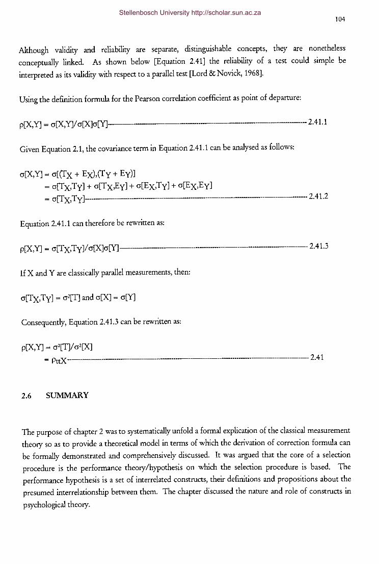
104
Although validity and reliability are separate, distinguishable concepts, they are nonetheless
conceptually linked. As shown below [Equation 2.41] the reliability of a test could simple be
interpreted as its validity with respect to a parallel test [Lord & Novick, 1968].
Using the definition formula for the Pearson correlation coefficient as point of departure:
p[X,Y] = cr[X,Y]/ cr[X]cr[Y]-------------------------------------------- 2.41.1
Given Equation 2.1, the covariance term in Equation 2.41.1 can be analysed as follows:
cr[X,Y] = cr[(fx + E:x),(Ty + Ey)]
= cr[Tx,Ty] + cr[Tx,Ey] + cr[Ex,Ty] + cr[Ex,Ey]
= cr[T x, T y ]------------------------------------------------------------------------------------------- 2. 41.2
Equation 2.41.1 can therefore be rewritten as:
p[X,Y] = cr[T x, T y ]/ cr[X]cr[Y] ------------------------------------------------------------------------------------- 2. 41.3
If X and Y are classically parallel measurements, then:
cr[Tx,Ty] = cr2[T] and cr[X] = cr[Y]
Consequently, Equation 2.41.3 can be rewritten as:
p[X,Y] = cr2[T]/ cr2[X]
= PttX ------------------------------------------------------------------------------------------------------- 2. 41
2.6 SUMMARY
The purpose of chapter 2 was to systematically unfold a formal explication of the classical measurement
theoty so as to provide a theoretical model in terms of which the derivation of correction formula can
be formally demonstrated and comprehensively discussed. It was argued that the core of a selection
procedure is the performance theoty /hypothesis on which the selection procedure is based. The
performance hypothesis is a set of interrelated constructs, their definitions and propositions about the
presumed interrelationship between them. The chapter discussed the nature and role of constructs in
psychological theory.
Stellenbosch University http://scholar.sun.ac.za
105
Justification of a selection procedure requires empirical confirmation of the validity of propositions
contained in the performance hypothesis. To empirically investigate the validity of such a performance
hypothesis, however, requires information on the constructs comprising the hypothesis. Due to the
abstract character of constructs, information on their state or level can be estimated only from their
effects. Thus measurement of constructs by necessity is of an indirect, inferential nature, through the
observation of indicants of the construct assumed or demonstrated to be related to the property. The
chapter examined and discussed the nature of psychological measurement.
The acceptance of operationalism as a solution to the measurement problem posed by the abstract
nature of psychological constructs rests on the supposition that inter- and intra-individual variance in
the observed indicant can be explained solely in terms of differences in the underlying construct of
interest. Although this represents a practically unattainable ideal, it nevertheless defines the objective of
perfectly controlled measurement in which all extraneous variables are controlled. Control is pursued
through two processes aimed at either removing the irrelevant variables or keeping the irrelevant
variable constant; the effect of both being that the variables no longer produce variance in observed
scores. The two processes in question are standardisation and test construction/item analysis. Perfect
control, however, is never achieved. The question, consequently, arises to what extent these processes
did succeed in controlling extraneous variance. Reliability and validity constitute two evaluatory
standards employed to answer this question. The chapter defined reliability and subsequently presented
the derivation of a number of reliability coefficients. In addition the chapter defined validity and
presented the criterion-related validity coefficient and its interpretation.
Stellenbosch University http://scholar.sun.ac.za
CHAPTER3
SEPARATE AND COMBINED CORRECTIONS TO THE VALIDITY COEFFICIENT
FOR THE ATTENUATING EFFECT OF THE UNRELIABILITY OF MEASUREMENTS
AND RESTRICTION OF RANGE
The purpose of the following chapter is firstly to systematically motivate the need for corrections to the
validity coefficient for the attenuating effect of the unreliability of the measurements and/ or restriction
of range. Subsequently the derivation of the various currently available correction formula are
discussed and the conditions under which their application would be appropriate.
3.1. THE NEED FOR CORRECTIONS TO THE VALIDITY COEFFICIENT FOR
THE ATTENUATING EFFECT OF THE UNRELIABILITY OF
MEASUREMENTS AND RESTRICTION OF RANGE
The process of validating a selection procedure in essence refers to a simulation of the selection
procedure so as to generate the empirical evidence needed to construct a convincing argument in terms
of which the appropriateness of the inferences, decisions and actions based on test scores in the
context of actual application can be justified [Guion, 1991; Kane, 1992; Messick, 19 89]. Inferences,
decisions and actions based on test scores are the outcomes of an implicit or explicit interpretive
argument [Kane, 1992]. At the core of the argument lies an array of hypothesis constituting a tentative
theory of work performance. Consequently, what needs to be validated for the applicant population is
the hypothesis that variance in ultimate criterion performance [Blum & Naylor, 1968] can be inferred
from scores on the selection tests [Guion, 1991]. The credibility of assertions on the validity of the
performance hypothesis in tum hinges on the unassailableness of the research methodology in terms of
which these hypothesis are empirically investigated. Cook, Campbell and Peracchio [1991] identify four
types of validity that, to the extent that they are threatened, render the research argument vulnerable to
questioning and consequently jeopardise the credibility of assertions on the validity of the performance
hypothesis. The degree of confidence with which variance in the dependent/ criterion construct can be
explained in terms of one or more hypothesised independent constructs is contingent on the extent to
which the research methodology/research design controls threats to the following four kinds of validity
[Cook, Campbell & Peracchio, 1992]:
);;> statistical conclusion validity;
);;> construct validity;
);;> internal validity; and
);;> external validity.
Stellenbosch University http://scholar.sun.ac.za
107
Statistical conclusion validity, a neologism created with some self-confessed trepidation by Cook,
Campbell and Peracchio [1991], refers to the validity of conclusions/ decisions on the attributability of
the observed sample results [i.e. covariance or difference] to chance. Construct validity refers to the
validity with which the measurement operations designed to provide an empirical grasp on the
dependent and independent constructs of interest, do in fact measure these constructs as constitutively
defined. Internal validity refers to the validity of the inference that variance in the dependent/ criterion
variable would be increased/ decreased by an increase/ decrease in the variance of the hypothesised
independent variable. Internal validity is consequently concerned with the question whether the
observed covariance between X-as measured [or X-as manipulated] andY-as measured can logically be
explained in terms of a cause-effect relationship. External validity concerns the generalisability of
research findings across times, conditions and individuals [Campbell & Stanley, 1963; Cook, Campbell
& Peracchio, 1991]. In an applied context external validity refers to the transportability of the research
findings to the area of application, that is to the [problem] area that motivated the research in the first
place.
The primary objective driving validation research is the accumulation of [credible] empirical evidence in
terms of which the appropriateness of the inferences, decisions and actions based on test scores in the
context of actual application can be justified [Guion, 1991; Kane, 1992; Messick, 1989]. The focus of
validation research thus falls on the actual utilisation of the selection procedure. The times, conditions
and individuals to which the validation research findings should be transported are consequently those
defining the area of actual application. Should the conditions and individuals characterising the
validation study in one or more respects not reflect those that would apply at the time of actual
application and, should the validation results be sensitive to the features that differ across the areas of
analysis and application, the transportability of the research evidence becomes questionable [i.e. the
external validity of the validation design would be low]. Consequently the credibility of the argument in
terms of which the validation researcher aims to justify the use of the selection procedure, is reduced
due to the questionable relevance of the validation evidence mustered. Previously the following
specific threats to the external validity of a validation research design were distinguished [Campbell,
1991; Lord & Novick, 1968; Tabachnick & Fidell, 1989;]:
~ the extent to which the actual or operationalised criterion contains random
measurement error;
~ the extent to which the actual or operationalised criterion is systematically biased;
i.e. the extent to which the actual criterion is deficient and/ or contaminated [Blum
& Naylor, 1968];
~ the extent to which the validation sample is an unrepresentative, biased, sample
from the applicant population in terms of homogeneity and specific attributes [e.g.
motivation, knowledge/ experience]; and
Stellenbosch University http://scholar.sun.ac.za
108
);;- the extent to which the sample size and the sample size to number of predictors
ratio allow capitalisation on chance and thus overfitting of data.
At the core of the to be constructed argument lies an array of hypotheses constituting a tentative theory
of work performance. Thus, what needs to be validated for the applicant population, is the hypothesis
that variance in ultimate [i.e. no contamination and no deficiency] criterion performance [Blum &
Naylor, 1968] can be explained in terms of variance in scores obtained from selection tests [Guion,
1991] representing construct valid operationalisations of the independent constructs suggested by the
hypothesised theory of work performance. The traditional statistical parameter in terms of which the
array of operationalised research hypotheses would normally be translated into statistical hypotheses, is
the Pearson correlation coefficient. Validation research thus essentially represents an attempt to obtain
an unbiased estimate of the parametric validity coefficient from the sample statistic derived from the
validation study. The foregoing argument thus translates to the notion that should factors exist that
bias the sample estimate of the parameter it would render the argument developed in defense of the
selection procedure vulnerable to attack except if such factors would be formally incorporated in the
psychometric defense of the selection procedure.
Aside from criterion deficiency and sample unrepresentativeness [i.e. the initial, unrestricted applicant
group represents an unrepresentative sample from the applicant population], it is possible to statistically
correct for all the other aforementioned threats to external validity of a validation design, provided the
required information is in fact available [which in principle is possible, although unlikely]. The need for
these corrections to the validity coefficient are motivated in terms of threats to the external validity of
the research design characterising a validation study. The obtained validity coefficient cannot, without
appropriate corrections, be considered an unbiased estimate of the parametric validity coefficient of
interest. The parameter of interest is the correlation coefficient obtained when the sample weights
derived from a representative sample are applied to the applicant population and the weighted
composite score would be correlated with error-free measurements [i.e. no intermediate criterion
contamination [random or systematic] or deficiency] of the [effectively ultimate] criterion for the
applicant population [Campbell, 1991]. Guion [1991, p. 351] expresses the importance of considering
the transportability of the sample validation evidence to the actual area of application as follows:
Use of a sample statistic to estimate the population parameter is ordinarily accepted if the measurements are
reliable, the sample large, and the sample of that population unbiased. These conditions are not routinely
found in validation research. Questions of research design are, ultimately, questions of how and whether
methods of data collection and data analysis permit inferences from the sample at hand about a larger
applicant population.
J
Stellenbosch University http://scholar.sun.ac.za
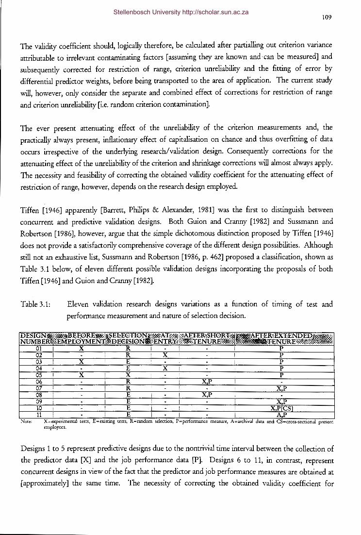
109
The validity coefficient should, logically therefore, be calculated after partialling out criterion variance
attributable to irrelevant contaminating factors [assuming they are known and· can be measured] and
subsequently corrected for restriction of range, criterion unreliability and the fitting of error by
differential predictor weights, before being transported to the area of application. The current study
will, however, only consider the separate and combined effect of corrections for restriction of range
and criterion unreliability [i.e. random criterion contamination].
The ever present attenuating effect of the unreliability of the cntenon measurements and, the
practically always present, inflationary effect of capitalisation on chance and thus overfitting of data
occurs irrespective of the underlying research/validation design. Consequently corrections for the
attenuating effect of the unreliability of the criterion and shrinkage corrections will almost always apply.
The necessity and feasibility of correcting the obtained validity coefficient for the attenuating effect of
restriction of range, however, depends on the research design employed.
Tiffen [1946] apparently [Barrett, Philips & Alexander, 1981] was the first to distinguish between
concurrent and predictive validation designs. Both Guion and Cranny [1982] and Sussmann and
Robertson [1986], however, argue that the simple dichotomous distinction proposed by Tiffen [1946]
does not provide a satisfactorily comprehensive coverage of the different design possibilities. Although
still not an exhaustive list, Sussmann and Robertson [1986, p. 462] proposed a classification, shown as
Table 3.1 below, of eleven different possible validation designs incorporating the proposals of both
Tiffen [1946] and Guion and Cranny [1982].
Table 3.1:
employees.
Eleven validation research designs vanatlons as a function of timing of test and
performance measurement and nature of selection decision.
Designs 1 to 5 represent predictive designs due to the nontrivial time interval between the collection of
the predictor data [X] and the job performance data [P]. Designs 6 to 11, in contrast, represent
concurrent designs in view of the fact that the predictor and job performance measures are obtained at
[approximately] the same time. The necessity of correcting the obtained validity coefficient for
Stellenbosch University http://scholar.sun.ac.za
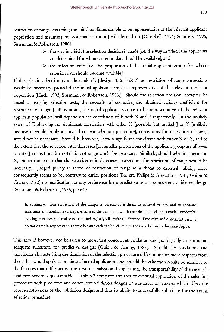
110
restriction of range [assuming the initial applicant sample to be representative of the relevant applicant
population and assuming no systematic attrition] will depend on [Campbell, 1991; Schepers, 1996;
Sussmann&Robertson, 1986]:
~ the way in which the selection decision is made [i.e. the way in which the applicants
are determined for whom criterion data should be available]; and
~ the selection ratio [i.e. the proportion of the initial applicant group for whom
criterion data should become available].
If the selection decision is made randomly [designs 1, 2, 6 & 7] no restriction of range corrections
would be necessary, provided the initial applicant sample is representative of the relevant applicant
population [Huck, 1992; Sussmann & Robertson, 1986;]. Should the selection decision, however, be
based on existing selection tests, the necessity of correcting the obtained validity coefficient for
restriction of range [still assuming the initial applicant sample to be representative of the relevant
applicant population] will depend on the correlation of E with X and P respectively. In the unlikely
event of E showing no significant correlation with either X [possible but unlikely] or Y [unlikely
because it would imply an invalid current selection procedure], corrections for restriction of range
would not be necessary. Should E, however, show a significant correlation with either X or Y, and to
the extent that the selection ratio decreases [i.e. smaller proportions of the applicant group are allowed
to enter], corrections for restriction of range would be necessary. Similarly, should selection occur on
X, and to the extent that the selection ratio decreases, corrections for restriction of range would be
necessary. Judged purely in terms of restriction of range as a threat to external validity, there
consequently seems to be, contrary to earlier positions [Barrett, Philips & Alexander, 1981; Guion &
Cranny, 1982] no justification for any preference for a predictive over a concurrent validation design
[Sussmann & Robertson, 1986, p. 464]:
In summary, when restriction of the sample is considered a threat to external validity and to accurate
estimation of population validity coefficients, the manner in which the selection decision is made - randomly,
existing tests, experimental tests - can, and logically will, make a difference. Predictive and concurrent designs
do not differ in respect of this threat because each can be affected by the same factors to the same degree.
This should however not be taken to mean that concurrent validation designs logically constitute an
adequate substitute for predictive designs [Guion & Cranny, 1982]. Should the conditions and
individuals characterising the simulation of the selection procedure differ in one or more respects from
those that would apply at the time of actual application and, should the validation results be sensitive to
the features that differ across the areas of analysis and application, the transportability of the research
evidence becomes questionable. Table 3.2 compares the area of eventual application of the selection
procedure with predictive and concurrent validation designs on a number of features which affect the
representativeness of the validation design and thus its ability to successfully substitute for the actual
selection procedure.
Stellenbosch University http://scholar.sun.ac.za
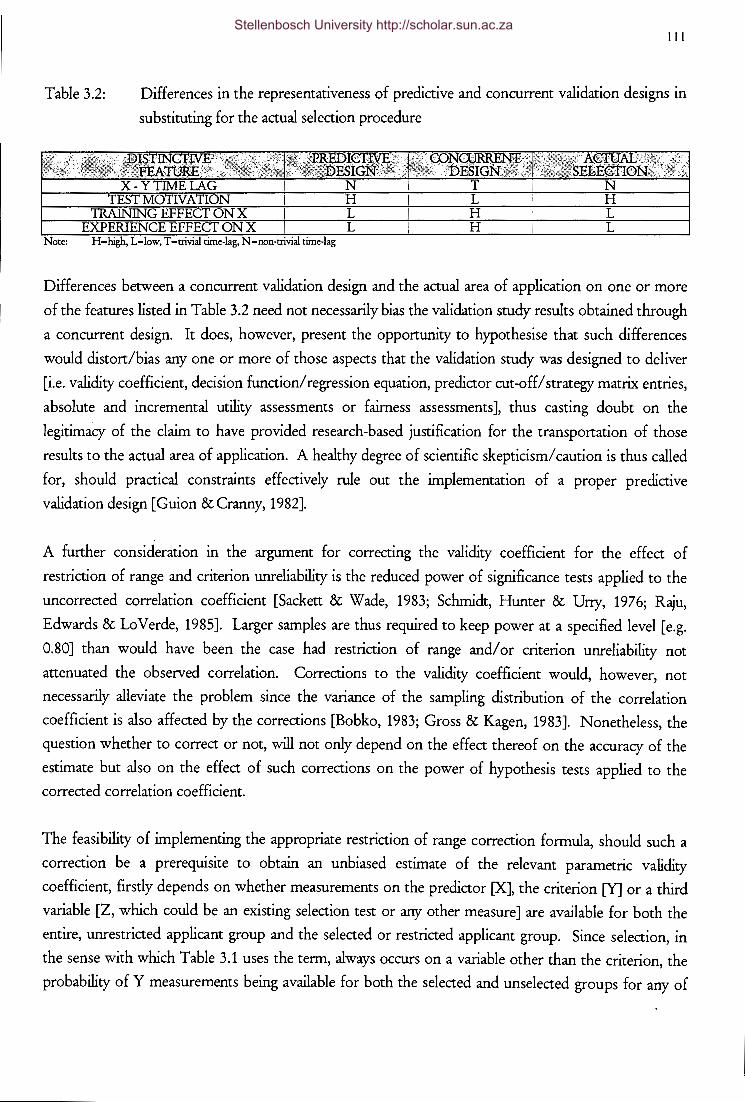
Table 3.2:
Ill
Differences in the representativeness of predictive and concurrent validation designs in
substituting for the actual selection procedure
Differences between a concurrent validation design and the actual area of application on one or more
of the features listed in Table 3.2 need not necessarily bias the validation study results obtained through
a concurrent design. It does, however, present the opportunity to hypothesise that such differences
would distort/bias any one or more of those aspects that the validation study was designed to deliver
[i.e. validity coefficient, decision function/ regression equation, predictor cut-off/ strategy matrix entries,
absolute and incremental utility assessments or fairness assessments], thus casting doubt on the
legitimacy of the claim to have provided research-based justification for the transportation of those
results to the actual area of application. A healthy degree of scientific skepticism/ caution is thus called
for, should practical constraints effectively rule out the implementation of a proper predictive
validation design [Guion & Cranny, 1982].
A further consideration in the argument for correcting the validity coefficient for the effect of
restriction of range and criterion unreliability is the reduced power of significance tests applied to the
uncorrected correlation coefficient [Sackett & Wade, 1983; Schmidt, Hunter & Uny, 1976; Raju,
Edwards & LoVerde, 1985]. Larger samples are thus required to keep power at a specified level [e.g.
0.80] than would have been the case had restriction of range and/ or criterion unreliability not
attenuated the observed correlation. Corrections to the validity coefficient would, however, not
necessarily alleviate the problem since the variance of the sampling distribution of the correlation
coefficient is also affected by the corrections [Bobko, 1983; Gross & Kagen, 1983]. Nonetheless, the
question whether to correct or not, will not only depend on the effect thereof on the accuracy of the
estimate but also on the effect of such corrections on the power of hypothesis tests applied to the
corrected correlation coefficient.
The feasibility of implementing the appropriate restriction of range correction formula, should such a
correction be a prerequisite to obtain an unbiased estimate of the relevant parametric validity
coefficient, firstly depends on whether measurements on the predictor [X], the criterion [Y] or a third
variable [Z, which could be an existing selection test or any other measure] are available for both the
entire, unrestricted applicant group and the selected or restricted applicant group. Since selection, in
the sense with which Table 3.1 uses the term, always occurs on a variable other than the criterion, the
probability of Y measurements being available for both the selected and unselected groups for any of
Stellenbosch University http://scholar.sun.ac.za
112
the eleven designs shown in Table 3.1, is zero. Third variable [Z] scores being available depends on
whether selection occurred on a third variable and whether the nature of the third variable is known.
Predictor [X] scores would be available if:
).- selection is directly based on X; or
).- the predictor is administrated before selection at random or based on a third
variable occurs.
The feasibility [or probably more appropriately termed, expediency] of implementing the appropriate
restriction of range correction formula, however, is also dependent on the extent to which the linearity
and homoscedasticity assumptions underlying the Pearson-Lawley correction formula [Campbell, 1991;
Huck, 1992; Olsen & Becker, 1983; Schepers, 1996] can be assessed and the extent to which they are
satisfied by the data set.
The assumption of no attrition is clearly unrealistic. In all eleven validation designs attrition would, to
the extent that it occurred, necessitate [additional] restriction of range corrections [assuming random
attrition to be extremely unlikely]. The appropriate correction should be feasible, as long as it was
known whether attrition occurred directly on job performance or on a third variable and Y or Z
measurements for both the restricted and unrestricted groups were available. Criterion measurements
for both the restricted and unrestricted groups would be logically impossible for any one of the eleven
designs in Table 3.1. Criterion measures could, however, be in principle available for pre- and post
attntlon groups.
Should support for the performance hypothesis be found [i.e. should an array of significant correlations
be found], a description of the functional relationship between the criterion and a [linear] combination
of these [significant] predictors need to be inferred to serve as a decision rule for actual personnel
selection decisions. In addition descriptive evaluations of the effectiveness, utility and fairness of
selection decisions based on the derived decision rule are required. The decision rule and the
descriptions of the effectiveness, utility and fairness of selection decisions based on the derived
decision rule are, however, just like the validity coefficient, all derived via a simulation of the selection
procedure under conditions that differ from those prevailing at the eventual use of the selection
procedure. The decision rule and the descriptions of the effectiveness, utility and fairness of selection
decisions could, thus, just like the validity coefficient, be biased to such an extent that the
transportability thereof becomes problematic. Whether this is in fact the case, and if so, under what
conditions and to what extent bias is introduced, is not completely clear although partial details has
been published [Linn, 1983; Pearson, 1903;]. Furthermore, appropriate correction formula do not seem
to be generally available, but even if they were, the question would still remain whether there is any
merit in applying any of these statistical correction formula. The research objectives as outlined in
chapter 1 are thus thereby indicated.
Stellenbosch University http://scholar.sun.ac.za
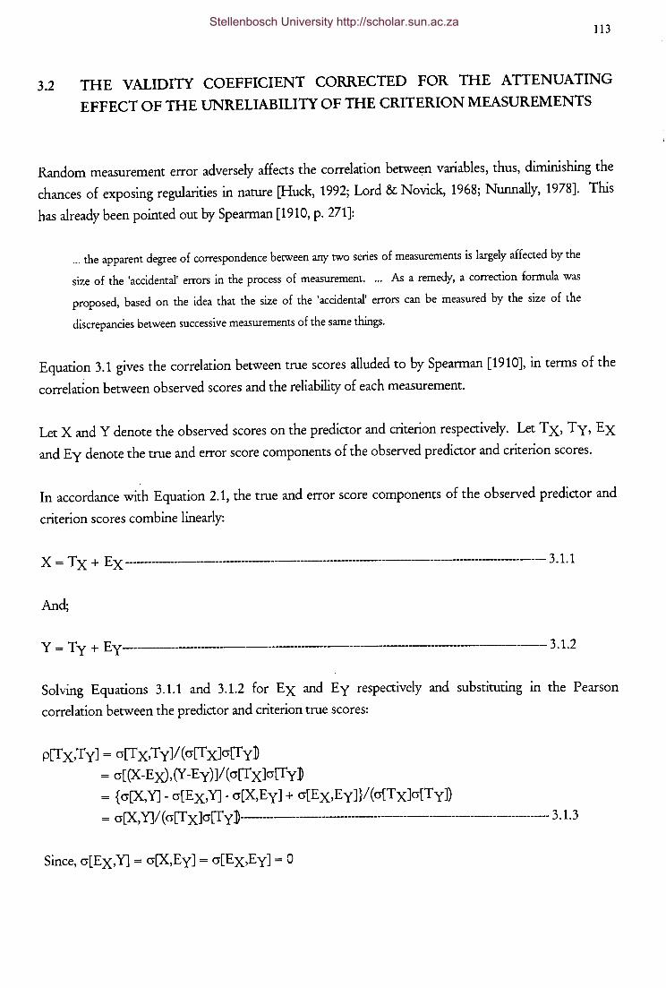
113
3.2 THE VALIDITY COEFFICIENT CORRECTED FOR THE ATTENUATING
EFFECT OF THE UNRELIABILITY OF THE CRITERION MEASUREMENTS
Random measurement error adversely affects the correlation between variables, thus, diminishing the
chances of exposing regularities in nature [Huck, 1992; Lord & Novick, 1968; Nunnally, 1978]. This
has already been pointed out by Spearman [1910, p. 271]:
... the apparent degree of correspondence between any two series of measurements is largely affected by the
size of the 'accidental' errors in the process of measurement. . .. As a remedy, a correction formula was
proposed, based on the idea that the size of the 'accidental' errors can be measured by the size of the
discrepancies between successive measurements of the same things.
Equation 3.1 gives the correlation between true scores alluded to by Spearman [1910], in terms of the
correlation between observed scores and the reliability of each measurement.
Let X andY denote the observed scores on the predictor and criterion respectively. Let Tx, Ty, Ex
and Ey denote the true and error score components of the observed predictor and criterion scores.
In accordance with Equation 2.1, the true and error score components of the observed predictor and
criterion scores combine linearly:
X = T X + EX --------------------------------------------------------------------------------------- 3 .1.1
And-'
Y = Ty + E y ------------------------------------------------------------------------ 3 .1.2
Solving Equations 3.1.1 and 3.1.2 for Ex and Ey respectively and substituting in the Pearson
correlation between the predictor and criterion true scores:
p[Tx,Ty] = cr[Tx,Ty]/(cr[Tx]cr[fy]
= cr[(X-Ex),(Y-Ey)]/(cr[Tx]cr[fy]
= {cr[X,Y]- cr[Ex,Y]- cr[X,Ey] + cr[Ex,Ey]}/(cr[TxJcr[Ty])
= cr[X,Y]/ ( cr[T xJcr[f y ]----------------------------------------------------------------- 3 .1. 3
Since, cr[Ex,Y] = cr[X,Ey] = cr[Ex,Ey] = 0
Stellenbosch University http://scholar.sun.ac.za
114
However, the correlation between the predictor and criterion observed scores is given by:
p[X,Y] = cr[X, Y]/ ( cr[X]cr[Y])------------------------------------------------------------------- 3 .1. 4
Isolating the covariance term in Equation 3.1.4:
cr[X,Y] = p[X,Y]cr[X]cr[Y]---------------------------------------- 3.1.5
Substituting Equation 3.1.5 in Equation 3.1.3:
p[Tx,Ty] = p[X,Y]cr[X]cr[Y]/(cr[TxJcr[fy]
= p[X, Y]/ { ( cr[T xJ/ cr[X]) ( cr[T y ]/ cr[Y]) } ------------------------------------------------------ 3 .1. 6
However, according to Equation 2.14, the correlation between two parallel measures indicate the
proportion true score variance, and hence:
cr[T xJ/ cr[X] = -/ p[Xip,XiqJ--------------------------------------------------------------------------------------- 3 .1. 7
and
cr[T y ]/ cr[Y] = -/ p[Y i P' Y i q] ------------------------------------------------------------------------------------------- 3 .1. 8
Substituting Equations 3.1.7 and 3.1.8 in Equation 3.1.6:
p[Tx,Ty] = p[X,Y]/ (-/p[XipXiqJ-/p[Yip,Yiq] ------------------------------------------------------------ 3.1.9
Write
p[XipXiqJ = PttX
and
Therefore the fully disattenuated validity coefficient can therefore be written as:
p[T x, T y] = p[X, Y]/ (-/ PttX-/ Ptt Y) ------------------------------------------------------------------------------ 3.1
Stellenbosch University http://scholar.sun.ac.za
115
Equation 3.1 is generally known as a correction/ estimation formula for the attenuating effect of the
unreliability of two measures on the correlation between their observed scores. Thus, if the reliabilities
of the two measures are known, then Equation 3.1 could be used to estimate the so called disattenuated
correlation [i.e. the correlation that would have been obtained if the true scores on the two measures
would have been correlated]. The disattenuated correlation provided by Equation 3.1 is, however, not
appropriate for applied selection validation research.
The correlation of interest in a validation study is the operational validity coefficient; the correlation
between the fallible predictor and actual job performance and not some fallible measure of
performance. Schmidt, Hunter & Urry [1976, p. 474] explain the necessity of correcting the validity
coefficient for the unreliability of the criterion only as follows:
Unreliability in the predictor is 'real' in the sense that, in actual selection use, one must use the test as it exists
- unreliability and all. Thus we do not correct the validity coefficient for unreliability in the test; it does no
good to compute the validity of a perfect reliable test since we do not have such a test available for use.
Unreliability in the criterion on the other hand, is not 'real' in the sense that it does not affect the operational
value of the selection test. Once the validation study is completed, the criterion measure is not used further.
In making selection decisions we use the test to make predictions of actual job performance, not performance
as measured on our imperfect criterion measure. Thus validity coefficients are, or should be, corrected for
unreliability in the criterion measure.
Through a procedure similar to that used to derive Equation 3.1, Equation 3.2 is obtained which
permits the estimation of the correlation between the observed score on one measure [typically the
predictor] and the true score on another measure [the criterion] from the correlation between the
observed scores on the two measures and the reliability of the second measure.
Let X andY denote the observed scores on the predictor and criterion respectively. Let Tx, Ty arrl
Ex and Ey denote the true and error score components of the observed predictor and criterion scores.
In accordance with Equation 2.1, the true and error score components of the observed predictor score
combine linearly:
X = Tx + Ex----------------------------------------------------------------------------------------------- 3.2.1
Solving Equation 3.2.1 for Ex and substituting in the Pearson correlation between the observed
predictor score and criterion true score:
p[X,Ty] = cr[X,Ty]/(cr[X]cr[fy]
Stellenbosch University http://scholar.sun.ac.za
= cr[(Tx + Ex),TyV(cr[X]cr[fy]
= {cr[fx,Ty] + cr[fy,Ex]}/(cr[X]cr[fy]
= cr[Tx,Ty ]/ ( cr[X]cr[fy] ------------------------------------------- 3 .2.2
Since cr[Ty,Ex] = 0
However:
cr[X,Y] = cr([fx-Ex],[fy+Ey]
= cr[Tx,Ty] + cr[Ex,Ty] + cr[Ey,Tx] + cr[Tx,Ty]
= cr[f x, T y ]------------------------------------------------------------------------------------- 3 .2.3
Substituting Equation 3.2.3 in Equation 3.2.2:
p[X,Ty] = cr[fx,Ty ]/ ( cr[X]cr[fy]
= cr[X,Y]/ ( cr[X]cr[f y] ----------------------------------------------------------------------------------- 3 .2. 4
However, the correlation between the predictor and criterion observed scores is given by:
p[X, Y] = cr[X, Y]/ ( cr[X]cr[Y])-------------------------------------------------------------------------------- 3 .2. 5
Isolating the covariance term in Equation 3.2.5:
cr[X,Y] = p[X, Y]cr[X]cr[Y]-------------------------------------------------------------------------------------------- 3 .2. 6
Substituting Equation 3.2.6 in Equation 3.2.4:
p[X, Ty] = p[X,Y]cr[X]cr[Y]/ ( cr[X]cr[T y]
= p[X,Y]cr[Y]/ cr[Ty]
= p[X,Y]/ ( cr[f y ]/ cr[Y])
= p[X,Y]/--./ PYip Yiq ----------------------------------------------------------------------- 3 .2.7
116
Since, according to Equation 2.14, the correlation between two parallel measures indicate the
proportion true score variance, and hence:
cr[Ty]/cr[Y] = --./PYipYiq
Stellenbosch University http://scholar.sun.ac.za
117
Write
PYip Yiq = Ptt Y
The partially disattenuated validity coefficient can therefore be written as:
p[X, T y] = PXY I...; Ptt y ----------------------------------------------------------------------------------- 3 .2
The behaviour of the partially disattenuated correlation coefficient as a function of the attenuated
correlation and the reliability coefficient is portrayed graphically in two dimensions in Figure 3.1 and in
three dimensions in Figure 3.2. The partially disattenuated correlation coefficient was mapped onto a
surface defined by 0.05 ::s;p[X,Y]::s;0.95 and O.OS::s;ptty::s;l.OO through a SAS program feeding a sample of
surface coordinates into Equation 3.2.
Figures 3.1 and 3.2 indicate that the utility of Equation 3.2 increases as PttY decreases. The observed
correlation coefficient p[X,Y] severely underestimates p[X, T y] when the reliability of the criterion is
low. At the upper end of the PttY -scale, however, the degree of underestimation becomes sufficiently
small to seriously question the utility of Equation 3.2.
3.3 THE VALIDITY COEFFICIENT CORRECTED FOR THE ATTENUATING
EFFECT OF EXPLICIT OR IMPLICIT RESTRICTION OF RANGE
3.3.1 Univariate Selection
If a nonzero correlation exists between X and Y within the applicant population, then the correlation
coefficient calculated for a random sample drawn from that population would, within the limits of
sampling error, approximate the parameter. That is E[rxyJ = p[X,Y]. If, however, the sample would
be selected conditional on the scores of the predictor X or the criterion Y or a third variable Z, then
the sample estimate will be systematically negatively biased; that is, E[rxy] < p[X,Y] [Campbell, 1991;
Huck, 1992; Olsen & Becker, 1983; Schepers, 1996]. In the typical [predictive] validation study some
form of the latter case normally prevails. According to Linn, Harnish and Dunbar [1981], Greener and
Osburn [1980], Campbell [1991] and Schepers [1996] the negative bias in the population correlation
coefficient estimate created by restriction of range can be quite severe for selection ratios and
[unrestricted] validity coefficients that are regularly encountered in validation research.
Stellenbosch University http://scholar.sun.ac.za
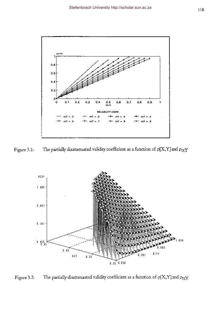
118
0.1 0.2 0.3 0.4 0.5 0.6 0.7 0.8 0.9 riX.YJ
RELIABILITY COEFF.
rttY = .2 -+- rttY = .3 -+- rttY = .4 -e- rttY = .5 _,._ rttY = .6 ~ rttY = .7 -&- rttY • .B
_,.._ mY • .9
Figure 3.1: The partially disattenuated validity coefficient as a function of p[X,Y] and PttY
1 . 0 00
0.05 0.050
Figure 3.2: The partially disattenuated validity coefficient as a function of p[X,Y] and PttY
Stellenbosch University http://scholar.sun.ac.za

119
All other factors kept constant, the more severe the selection process [i.e. the larger the proportion of
the total population with missing values on the incidental selection variable(s)] the stronger the
influence of restriction of range [Guion, 1991; Schepers, 1996]. Schepers [1996] reports that very high
and very low [unrestricted population] correlations are only slightly influenced by restriction of range.
Correlations in the middle range [i.e. 0,40- 0,80], however, are severely curtailed by restriction of range
[Schepers, 1996 ]. This would thus imply that the parametric predictive validity of the selection
procedure would be substantially misrepresented by the uncorrected sample result. The psychometric
problem confronting the validation researcher is to estimate the bivariate correlation for the
unrestricted applicant population from the available, biased data.
Pearson [1903] was the first to provide a procedure to correct for the attenuating effect of restriction of
range due to explicit or implicit selection. Lawley [1943] relaxed the assumptions required by the
Pearson [1903] procedure. Thorndike [1949] is credited with disseminating the Pearson-Lawley
procedure among psychometrists [Mendoza, Hart & Powell, 1991].
Considerable confusion and error can be avoided by distinguishing carefully between the different types
of selection. Pearson [1903] identified three different conditions under which estimation bias due to
selection could occur. From the work of Thorndike [1949; 1982] these three circumstances initially
became known as Cases 1, 2 and 3 [Ree, Caretta, Earles & Albert, 1994; Thorndike, 1949]. Thorndike
[1982] subsequently also refered to the three conditions under which estimation bias could occur as
Cases B, A and C [Olsen & Becker, 1983; Ree, Carretta, Earles & Albert, 1994; Thorndike, 1949;
Thorndike, 1982]. These three cases can be distinguished as follows:
>- Case 1[Case B]: the correlation to be corrected is between two variables X andY,
selection occurred [directly/explicitly] on the variable X [or Y] through complete
truncation on X at Xc [or on Y at Y cJ and both restricted and unrestricted variances
are known only for the incidental selection variable Y [or X];
>- Case 2 [Case A]: the correlation to be corrected is between two variables X andY,
selection occurred [directly I explicitly] on the variable X [or Y] through complete
truncation on X at Xc [or on Y at Y cJ and both restricted and unrestricted variances
are known only for the explicit selection variable X [or Y];
>- Case 3[i] [Case C[i]]: the correlation to be corrected is between two variables
X andY, selection occurred [directly/explicitly] on the variable Z [a single variable
or a composite] through complete truncation on Z at Zc [the truncation on Y and X
thus is incomplete] and both restricted and unrestricted variances are known only
for the explicit selection variable Z; and
>- Case 3[ii] [Case C[ii]]: the correlation to be corrected is between two variables
X andY, selection occurred [directly/ explicitly] on the variable Z through complete
Stellenbosch University http://scholar.sun.ac.za
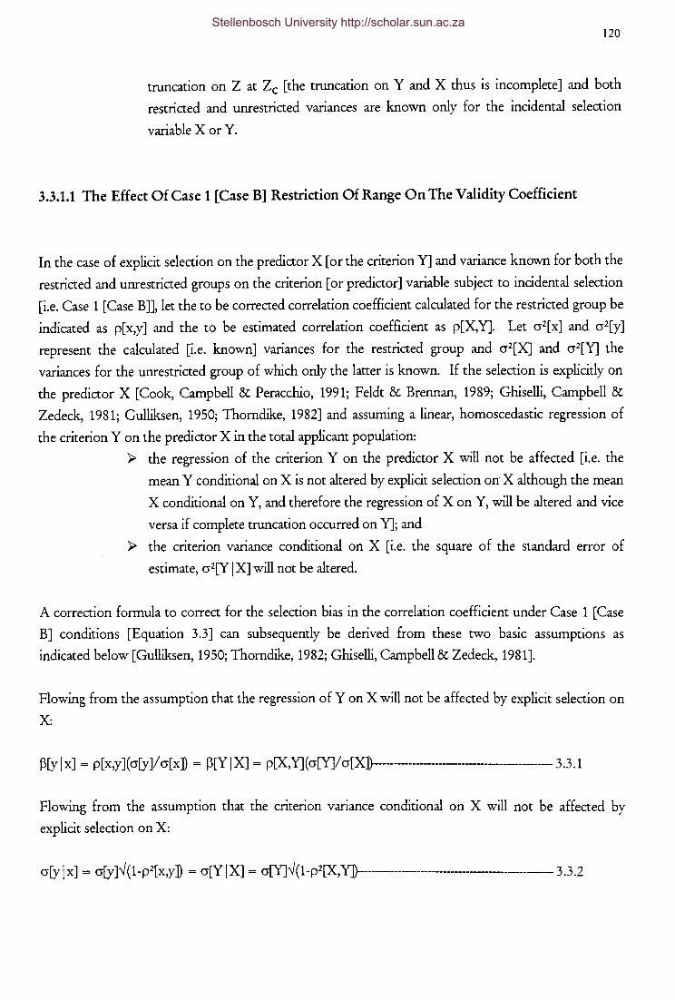
120
truncation on Z at Zc [the truncation on Y and X thus is incomplete] and both
restricted and unrestricted variances are known only for the incidental selection
variable X or Y.
3.3.1.1 The Effect Of Case 1 [Case B] Restriction Of Range On The Validity Coefficient
In the case of explicit selection on the predictor X [or the criterion Y] and variance known for both the
restricted and unrestricted groups on the criterion [or predictor] variable subject to incidental selection
[i.e. Case 1 [Case B]], let the to be corrected correlation coefficient calculated for the restricted group be
indicated as p[x,y] and the to be estimated correlation coefficient as p[X,Y]. Let cr2[x] and cr2[y]
represent the calculated [i.e. known] variances for the restricted group and cr2[X] and cr2[Y] the
variances for the unrestricted group of which only the latter is known. If the selection is explicitly on
the predictor X [Cook, Campbell & Peracchio, 1991; Feldt & Brennan, 1989; Ghiselli, Campbell &
Zedeck, 1981; Gulliksen, 1950; Thorndike, 1982] and assuming a linear, homoscedastic regression of
the criterion Y on the predictor X in the total applicant population:
};> the regression of the criterion Y on the predictor X will not be affected [i.e. the
mean Y conditional on X is not altered by explicit selection orr X although the mean
X conditional on Y, and therefore the regression of X on Y, will be altered and vice
versa if complete truncation occurred on Y]; and
};> the criterion variance conditional on X [i.e. the square of the standard error of
estimate, cr2[Y I X] will not be altered.
A correction formula to correct for the selection bias in the correlation coefficient under Case 1 [Case
B] conditions [Equation 3.3] can subsequently be derived from these two basic assumptions as
indicated below [Gulliksen, 1950; Thorndike, 1982; Ghiselli, Campbell & Zedeck, 1981].
Flowing from the assumption that the regression of Y on X will not be affected by explicit selection on
X:
~[y I x] = p[ x,y ]( cr[y ]/ cr[ x ]) = ~[Y I X] = p[X,Y]( cr[YJ/ cr[X]}------------------------------------------ 3.3 .1
Flowing from the assumption that the criterion variance conditional on X will not be affected by
explicit selection on X:
cr[y I x] = cr[y ]v' ( 1-p2[ x,y ]) = cr[Y I X] = cr[Y]v' ( 1-p2[X, Y]}--------------------------------------------------- 3. 3.2
Stellenbosch University http://scholar.sun.ac.za
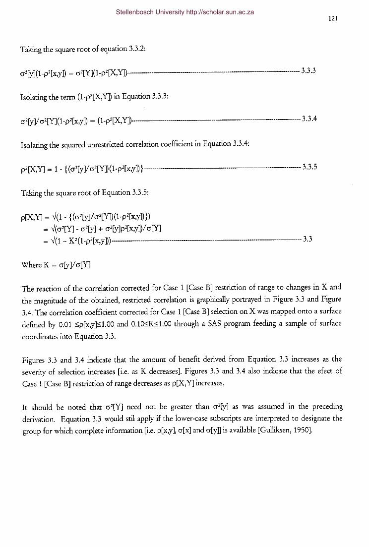
121
Taking the square root of equation 3.3.2:
cr2[y] ( 1-p2[ x,y ]) = cr2[YJ ( 1-p2[X,Y])------------------------------------------------------------------------- 3 .3 .3
Isolating the term (1-p2[X,Y] in Equation 3.3.3:
cr2[y ]/ cr2[YJ ( 1-p2[ x,y ]) = ( 1-p2[X, Y])------------------------------------------------------------------- 3 .3. 4
Isolating the squared unrestricted correlation coefficient in Equation 3.3.4:
p2[X,Y] = 1 _ { ( cr2[y ]/ cr2[Y]) ( 1-p2[ x,y ]) } ------------------------------------------------------------------- 3. 3. 5
Taking the square root of Equation 3.3.5:
p[X,Y] = --./(1- {(cr2[y]/cr2[YJ)(1-p2[x,y])})
= --J ( cr2[YJ _ cr2[y] + crz[y Jp2[ x,y ]/ cr[YJ
= --./ ( 1 - K 2 ( 1-p2 [ x, y]) ----------------------------------------------------------------------------------------- 3 . 3
Where K = cr[y ]/ cr[YJ
The reaction of the correlation corrected for Case 1 [Case B] restriction of range to changes inK and
the magnitude of the obtained, restricted correlation is graphically portrayed in Figure 3.3 and Figure
3.4. The correlation coefficient corrected for Case 1 [Case B] selection on X was mapped onto a surface
defined by 0.01 ~p[x,y]~l.OO and 0.10~K~l.OO through a SAS program feeding a sample of surface
coordinates into Equation 3.3.
Figures 3.3 and 3.4 indicate that the amount of benefit derived from Equation 3.3 increases as the
severity of selection increases [i.e. as K decreases]. Figures 3.3 and 3.4 also indicate that the efect of
Case 1 [Case B] restriction of range decreases as p[X,Y] increases.
It should be noted that cr2[YJ need not be greater than cr2[y] as was assumed in the preceding
derivation. Equation 3.3 would stil apply if the lower-case subscripts are interpreted to designate the
group for which complete information [i.e. p[ x,y ], cr[ x] and cr[y] is available [ Gulliksen, 19 50].
Stellenbosch University http://scholar.sun.ac.za
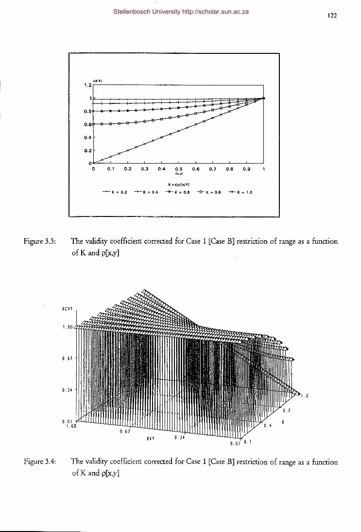
Figure 3.3:
Figure 3.4:
122
riX.YI 1.2r------------------------------------------,
0.4
0.2
0.1 0.2 0.3 0.4 0.5 0.6 0.7 0.8 0.9 rlr.,yl
K = s(y)/s[YJ
- K = 0.2 -+- K = 0.4 ""*- K = 0.6 -e- K = 0.8 """*- K = 1.0
The validity coefficient corrected for Case 1 [Case B] restriction of range as a function
of K and p[x,y]
1.0
The validity coefficient corrected for Case 1 [Case B] restriction of range as a function
of K and p[x,y]
Stellenbosch University http://scholar.sun.ac.za
123
3.3.1.2 The Effect Of Case 2 [Case A] Restriction Of Range On The Validity Coefficient
In the more common case of explicit selection on the predictor X and variance known for both the
restricted and unrestricted groups on the predictor variable subject to direct selection [i.e. Case 2 [Case
A]], let the to be corrected correlation coefficient calculated for the restricted group again be indicated
as p[x,y] and the to be estimated correlation coefficient still as p[X,Y]. Let cr2[x] and cr2[y] represent the
calculated [i.e. known] variances for the restricted group and cr2[X] and cr2[Y] the variances for the
unrestricted group of which only the former is known.
If the selection is explicitly on the predictor X the same two assumptions applicable to Case 1 [Case B]
also apply to Case 2 [Case A]. A correction formula to correct for the selection bias in the correlation
coefficient under Case 2 [Case A] conditions [Equation 3.4] can subsequently be derived from these
two basic assumptions as indicated below [Gulliksen, 1950; Lord & Novick, 1968; Ghiselli, Campbell &
Zedeck, 1981; Thorndike, 1982].
Flowing from the assumption that the regression of Y on X will not be affected by explicit selection on
X:
~[y I x] = p[ x,y ]( cr[y ]I cr[ x ]) = ~[Y I X] = p[X,Y]( cr[Y]I cr[X]}----------------------------------------------- 3.4 .1
Flowing from the assumption that the criterion variance conditional on X will not be affected by
explicit selection on X:
cr[y I x] = cr[y ]v' ( 1-p2[x,y ]) = cr[Y I X] = cr[Y]v' ( 1-p2[X, Y]}------------------------------------------------- 3 .4 .2
Isolating the term (cr[Y]Icr[X]) in Equation 3.4.1:
cr[Y]I cr[X] = (p[ x,y ]cr[y ]) I ( cr[ x] p[X,Y]) ------------------------------------------------------------------ 3. 4. 3
Isolating the unrestricted criterion standard deviation in Equation 3.4.3:
cr[Y] = (p[ x,y ]cr[y ]cr[X]) I ( cr[ x ]p[X,Y]) ------------------------------------------------------------------------------ 3. 4. 4
Taking the square root of Equation 3.4.2 and substituting the unrestricted criterion standard deviation
in Equation 3.4.2 with Equation 3.4.4:
cr[y](1-p2[xy])~ = cr[Y](1-p2[X,Y])~
Stellenbosch University http://scholar.sun.ac.za
= { (p[ x,y ]cr[y ]cr[X])/ ( cr[ x ]p[X, Y]} ( 1-p2[X,Y]) V2..------------------------- 3. 4.5
Squaring Equation 3.4.5:
cr2[y](1-p2(xy ]) = { (p2(x,y]cr2[y ]cr2[X]/ (cr2(x]p2[X,Y])} (1-pl[X,Y]}------------------------- 3.4.6
Isolating the term (1-p2[xy]) in Equation 3.4.6:
(1-p2[xy]) = { (p2(x,y]cr2[X])/(cr2(x]p2[X,Y] }(1-pz[X,Y]-----------·--------------- 3.4.7
Cross multiplying Equation 3.4.7:
( 1-p2( xy ]) ( cr2(x ]p2[X,Y]) = (p2[ x,y ]cr2[X]) ( 1-p2[X,Y]}---------------------------------------------------------- 3.4. 8
Multiplying Equation 3.4.8 with 1/(p2[x,y]cr2[X])(1/p2[X,Y]):
cr2(x](1-p2(xy])/ (p2(x,y]cr2(X]) = (1-p2[XY])/ p2[X,Y] = (1/ p2[X,Y]) - 1------------------------------------------------------- 3.4.9
Simplifying the left-hand term in Equation 3.4.9:
(1/ p2[X,Y]) - 1 = cr[x](1-p2[xy])/(p2[x,y]cr2[X])
= (cr2[x]- cr2[x]p2[xy])/(p2[x,y]cr2[X])
= ( cr2[x ]/ p2[ x,y] - cr2[ x ]) I cr2[X]
= (cr2[x]/ cr2[X])(1/ p2[x,y]- 1) --------------------------------------------------------------- 3.4.10
124
Isolating the term (1/ p2[X,Y] in Equation 3.4.10, multiplying the right-hand side out and creating
(cr2[X]p2[x,y] as a common denominator:
(1/p2[X,Y]) = 1 + (cr2[x]/cr2[X](1/p2[x,y] -1)
= 1 + cr2[x ]/ ( cr2[X]p2[ x,y] - ( cr2[ x ]/ cr2[X])
= (cr2[X]p2[x,y] + cr2[x]- cr2[x]p2[x,y])/(cr2[X]p2[x,y])----------------------------------- 3.4.11
Isolating the square of the unrestricted correlation coefficient in Equation 3.4.11 through an inversion
of Equation 3.4.11:
p2[X,Y] = 1/ { (cr2[X]p2[x,y] + cr2[x]- cr2[x]p2[x,y])/(cr2[X]p2[x,y])} = (cr2[X]p2[x,y])/(cr2[X]p2[x,y] + cr2[x]- cr2[x]p2[x,y]}-------------------------------------- 3.4.12
J
Stellenbosch University http://scholar.sun.ac.za
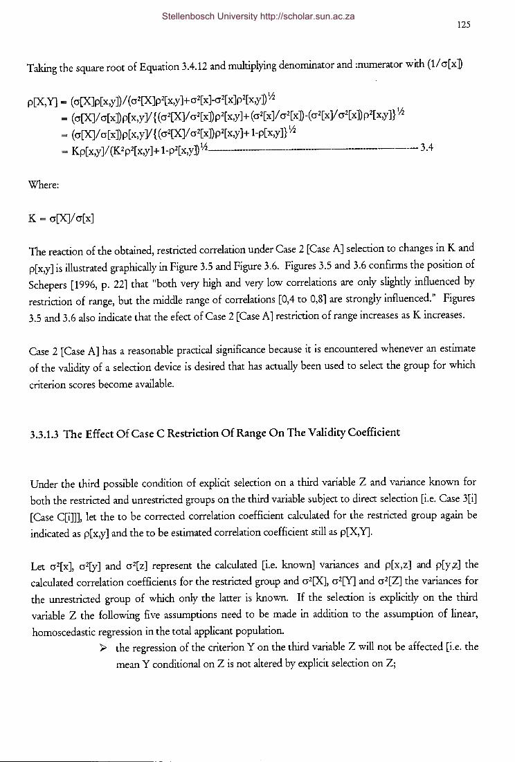
125
Taking the square root of Equation 3.4 .12 and multiplying denominator and :numerator with ( 11 cr[ X n
p[X,Y] = ( cr[X]p[ x,y ]) I ( cr2[X]p2[ x,y ]+ cr2[x ]-cr2[ x ]p2
[ x,y ]) lh
= (cr[X]/ cr[x])p[x,yV { (cr2[XJ/ cr2[x])p2[x,y]+ (cr2[x]/ cr2[x]-(cr2[x]/ cr2[x])p2[x,y]} lh
= (cr[X]/ cr[x])p[x,y V { (cr2[X]/ cr2[x])p2[x,y]+ 1-p[x,y]} lh
= Kp[ x,y ]/ (K 2p2[ x,y ]+ 1-p2[ x,y] lh-------------------------------------------- 3. 4
Where:
K = cr[X]/ cr[ x]
The reaction of the obtained, restricted correlation under Case 2 [Case A] selection to changes inK and
p[x,y] is illustrated graphically in Figure 3.5 and Figure 3.6. Figures 3.5 and 3.6 confirms the position of
Schepers [1996, p. 22] that "both very high and very low correlations are only slightly influenced by
restriction of range, but the middle range of correlations [0,4 to 0,8] are strongly influenced." Figures
3.5 and 3.6 also indicate that the efect of Case 2 [Case A] restriction of range increases asK increases.
Case 2 [Case A] has a reasonable practical significance because it is encountered whenever an estimate
of the validity of a selection device is desired that has actually been used to select the group for which
criterion scores become available.
3.3.1.3 The Effect Of Case C Restriction Of Range On The Validity Coefficient
Under the third possible condition of explicit selection on a third variable Z and variance known for
both the restricted and unrestricted groups on the third variable subject to direct selection [i.e. Case 3[i]
[Case C[i]]], let the to be corrected correlation coefficient calculated for the restricted group again be
indicated as p[x,y] and the to be estimated correlation coefficient still as p[X,Y].
Let cr2[x], cr2[y] and cr2[z] represent the calculated [i.e. known] variances and p[x,z] and p[y,z] the
calculated correlation coefficients for the restricted group and cr2[X], cr2[Y] and cr2[Z] the variances for
the unrestricted group of which only the latter is known. If the selection is explicitly on the third
variable Z the following five assumptions need to be made in addition to the assumption of linear,
homoscedastic regression in the total applicant population.
);;> the regression of the criterion Y on the third variable Z will not be affected [i.e. the
mean Y conditional on Z is not altered by explicit selection on Z;
Stellenbosch University http://scholar.sun.ac.za
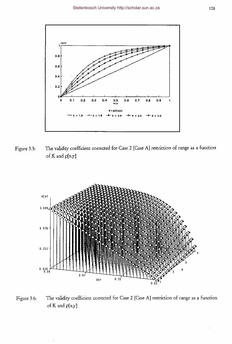
Figure 3.5:
Figure 3.6:
126
0.8
0.6
0.4
0.2
0.1 0.2 0.3 0.4 0.5 0.6 0. 7 0.8 0.9 rtx.y)
K e s(X]/s(x]
- K • 1.0 -+- K ~ 1.5 -*- K • 2.0 -e- K • 2.5 -*- K • 3.0
The validity coefficient corrected for Case 2 [Case A] restriction of range as a function
of K and p[x,y]
The validity coefficient corrected for Case 2 [Case A] restriction of range as a function
of K and p[x,y]
Stellenbosch University http://scholar.sun.ac.za
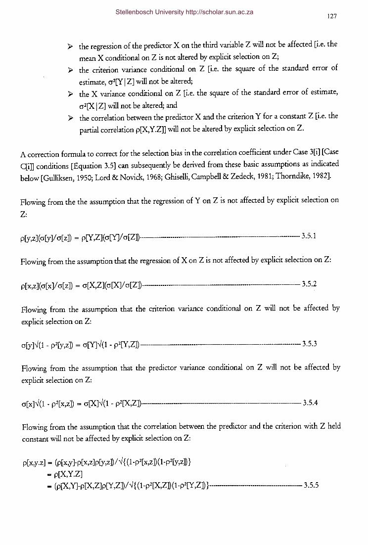
127
);> the regression of the predictor X on the third variable Z will not be affected [i.e. the
mean X conditional on Z is not altered by explicit selection on Z;
);> the criterion variance conditional on Z [i.e. the square of the standard error of
estimate, cr2[Y I Z] will not be altered;
);> the X variance conditional on Z [i.e. the square of the standard error of estimate,
cr2[X I Z] will not be altered; and
);> the correlation between the predictor X and the criterion Y for a constant Z [i.e. the
partial correlation p[X,Y.Z]] will not be altered by explicit selection on Z.
A correction formula to correct for the selection bias in the correlation coefficient under Case 3[i] [Case
qi]] conditions [Equation 3.5] can subsequently be derived from these basic assumptions as indicated
below [Gulliksen, 1950; Lord & Novick, 1968; Ghiselli, Campbell & Zedeck, 1981; Thorndike, 1982].
Flowing from the the assumption that the regression of Y on Z is not affected by explicit selection on
Z:
p[y,z] ( cr[y ]/ cr[ z ]) = p[Y ,Z] ( cr[Y]/ cr[Z])-------------------------------------------------------------------------- 3. 5.1
Flowing from the assumption that the regression of X on Z is not affected by explicit selection on Z:
p[ x,z ]( cr[ x ]/ cr[ z ]) = cr[X,Z]( cr[X]/ cr[Z])----------------------------------------------------------------------- 3 .5.2
Flowing from the assumption that the criterion variance conditional on Z will not be affected by
explicit selection on Z:
cr[y ].,, ( 1 - p2[y ,z ]) = cr[Y]--J ( 1 - p2[Y ,Z]) ------------------------------------------------------------------------- 3. 5. 3
Flowing from the assumption that the predictor variance conditional on Z will not be affected by
explicit selection on Z:
cr[x]--J(1 - p2[x,z]) = cr[X]--J(1 - p2[X,Z])----------------------------------------------------------------- 3.5.4
Flowing from the assumption that the correlation between the predictor and the criterion with Z held
constant will not be affected by explicit selection on Z:
p[x,y.z] = (p[x,y]-p[x,z]p[y,z])/--J{ (1-p2[x,z])(1-p2[y,z])}
= p[X,Y.Z]
= (p[X,Y]-p[X,Z]p[Y,Z])/.,! { ( 1-p2[X,Z]) (1-p2[Y,Z]) }-------------------------------------------- 3.5.5
Stellenbosch University http://scholar.sun.ac.za
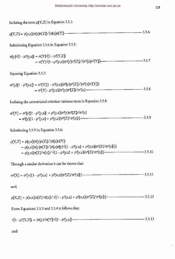
128
Isolating the term p[Y,Z] in Equation 3.5.1:
p[Y ,Z] = p[y,z ]( cr[y ]cr[Z]) I ( cr[ z ]cr[Y])------------------------------------------------------- 3. 5. 6
Substituting Equation 3.5.6 in Equation 3.5.3:
cr[y]--J(1 - p2[y,z]) = cr[Y]--J(1 - p2[Y,Z]) = cr[Y]--J(1 - p2[y,z](cr2[y]cr2[Z])I(cr2[z]cr2[Y])}---------------------------- 3.5.7
Squaring Equation 3.5.7:
cr2[y](1- p2[y,z] = cr2[Y](1- p2[y,z](cr2[y]cr2[Z])I(cr2[z]cr2[Y])) = cr2[Y] - p2[y ,z] ( cr2[y ]cr2[Z]) I cr2[ z ]------------------------------------------------------- 3. 5. 8
Isolating the unrestricted criterion variance term in Equation 3.5.8:
cr2[Y] = cr2[y](1- p2[y,z]) + p2[y,z](cr2[y]cr2[Z])Icr2[z]
= cr2[y] { 1 - p2[y,z] + p2[y,z ]( cr2[Z]I cr2[ z ]) } ---------------------------------------------------------- 3 .5. 9
Substituting 3.5.9 in Equation 3.5.6:
p[Y ,Z] = p[y ,z] ( cr[y ]cr[Z]) I ( cr[ z ]cr[Y])
= p[y,z](cr[y]cr[Z])I(cr[z]cr[y]--J{1- p2[y,z] + p2(y,z](cr2[Z]Icr2[z])})
= p[y,z ]( cr[Z]I cr[ z ]) I --J { 1 - p2[y,z] + p2[y,z ]( cr2[Z]I cr2[ z ])}---------------------------------------- 3. 5.10
Through a similar derivation it can be shown that:
cr2[X] = cr2[x]{ 1 - p2[x,z] + p2[x,z](cr2[Z]I cr2[z]) }----------------------------------------------------------- 3.5.11
and;
p[X,Z] = p[x,z](cr[Z]Icr[z])I--J{1- p2[x,z] + p2[x,z](cr2[Z]Icr2[z])}----------------------------------- 3.5.12
From Equations 3.5.3 and 3.5.4 it follows that:
--J ( 1 - p2[Y ,Z]) = ( cr[y ]I cr[YJ) --J ( 1 - p2[y ,z ]) -------------------------------------------------------------------- 3. 5.13
and:
Stellenbosch University http://scholar.sun.ac.za
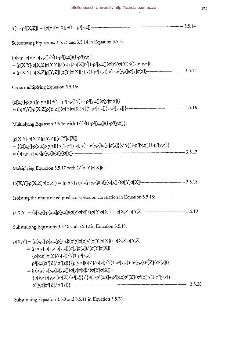
-,J(1- p2[X,Z]) = (cr[x]lcr[X])-,J(1- p2[x,z])----------· -------------------- 3 .5.14
Substituting Equations 3.5.13 and 3.5.14 in Equation 3.5.5:
(p[x,y ]-p[x,z]p[y,z])l -,J ( 1-p2[x,z ]) (1-p2[y,z ])
= (p[X,Y]-p[X,Z]p[Y,Z])I(cr[x]lcr[X])-,J(1-p2[x,z])(cr[yVcr[Y])-,J(1-p2[y,z])
= (p[X,Y]-p[X,Z]p[Y,Z])(cr[Y]cr[X])I { -,J(1-p2[x,z])-,J(1-p2[y,z]cr[y]cr[x]}--------------- 3.5.15
Cross multiplying Equation 3.5.15:
(p[x,y]-p[x,z]p[y,z]){-,J(1- p2[x,z])-,J(1- p2[y,z])(cr[y]cr[x])}
= (p[X,Y]-p[X,Z]p[Y,Z])(cr[Y]cr[X])-,J { (1-p2[x,z])(1-p2[y,z]) }------------------------------------- 3.5.16
Multiplying Equation 3.5.16 with 11 { -,J(1-p2[x,z])(1-p2[y,z]) }:
(p[X,Y]-p[X,Z]p[Y,Z]) ( cr[Y]cr[X]
= { (p[x,y]-p[x,z]p[y,z]) { -,J(1-p2[x,z])-,J(1-p2[y,z])cr[y]cr[x]} }1-,J { (1-p2[x,z])(1-p2[y,z])}
= (p[ x,y ]-p[ x,z ]p[y ,z ]) ( cr[y ]cr[ x ]}---------------------------------------------------------------------------- 3. 5.17
Multiplying Equation 3.5.17 with 11(cr[Y]cr[X]):
(p[X,Y]-p[X,Z]p[Y,Z]) = (p[ x,y ]-p[ x,z]p[y,z ]) ( cr[y ]cr[ x])l ( cr[Y]cr[X])----------------------------------- 3 .5.18
Isolating the unrestricted predictor-criterion correlation in Equation 3.5.18:
p[X, Y] = (p[ x,y ]-p[ x,z] p[y ,z ]) ( cr[y ]cr[ x ]) I ( cr[Y]cr[X]) + p[X,Z]p[Y,Z}--------------------------------- 3. 5.19
Substituting Equations 3.5.10 and 3.5.12 in Equation 3.5.19:
p[X,Y] = (p[ x,y ]-p[ x,z ]p[y,z ]) ( cr[y ]cr[ x ]) I ( cr[Y]cr[X]) + p[X,Z]p[Y,Z]
= (p[x,y ]-p[ x,z ]p[y,z] ( cr[y ]cr[ x ])I ( cr[Y]cr[X]) +
{ p[ x,z ]( cr[Z]I cr[ z ])I -,J ( 1-p2[ x,z]+
p2[x,z]cr2[Z]I cr2[z])} {p[y,z](cr[Z]I cr[z])I-,J(1-p2[y,z]+ p2[y,z]cr2[Z]I cr2[z])}
= (p[x,y]-p[x,z]p[y,z])(cr[y]cr[x])l(cr[Y]cr[X])+
{p[x,z]p[y,z](cr2[Z]I cr2[z]) }I { -,J(1-p2[x,z]+ p2[x,z]cr2[Z]I cr2[z])-,J(1-p2[y,z]+
p2[y,z ]cr2[Z]I cr2[ z ]) } ------------------------------------------------------------------------------ 3. 5.20
Substituting Equation 3.5.9 and 3.5.11 in Equation 3.5.20:
129 Stellenbosch University http://scholar.sun.ac.za
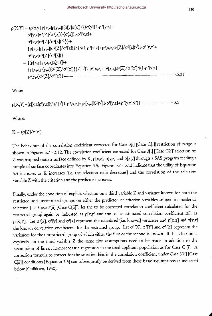
p[X,Y] = (p[x,y]-p[x,z]p[y,z](cr[y]cr[x])/ { (cr[y]{ 1-p2[y,z]+
pz[y,z ]cr2[Z]/ cr2[ z ]) } { cr[ x ]( 1-p2[x,z ]+
p2[x,z ]cr2[Z]/ cr2[ z] lh}} +
{ p[ x,z ]p[y,z ]( cr2[Z]/ cr2[ z ]) } I { -J ( 1-p2[ x,z ]+ p2[ x,z ]cr2[Z]/ cr2[ z ]) -J ( 1-p2[y,z ]+
p2[y,z]cr2[Z]/ cr2[z])}
= { (p[x,y ]-p[ x,z ]p[y ,z ]) +
{p[x,z]p[y,z](cr2[Z]/ cr2[z])} }/ { --J(1-p2[x,z]+ p2[x,z]cr2[Z]/ cr2[z])--J(1-p2[y,z]+
p2[y,z ]cr2[Z]/ cr2[ z ]) } ------------------------------------------------------------ 3 .5.21
Write:
p[X,Y]= (p[x,z]p[y,z]K2)/ { --J(1-p2[x,z]+ p2[x,z]K2)--J(1-p2[y,z]+ p2[y,z]K2) }------------------------- 3.5
Where:
K = ( cr[Z]/ cr[ z ])
130
The behaviour of the correlation coefficient corrected for Case 3[i] [Case C[i] restriction of range is
shown in Figures 3.7 - 3.12. The correlation coefficient corrected for Case 3[i] [Case C[i]] selection on
Z was mapped onto a surface defined by K, p[x,z], p[y,z] and p[x,y] through a SAS program feeding a
sample of surface coordinates into Equation 3.5. Figures 3.7- 3.12 indicate that the utility of Equation
3.5 increases as K increases [i.e. the selection ratio decreases] and the correlation of the selection
variable Z with the criterion and the predictor increases.
Finally, under the condition of explicit selection on a third variable Z and variance known for both the
restricted and unrestricted groups on either the predictor or criterion variables subject to incidental
selection [i.e. Case 3[ii] [Case qii]]], let the to be corrected correlation coefficient calculated for the
restricted group again be indicated as p[ x,y] and the to be estimated correlation coefficient still as
p[X,Y]. Let cr2[x], cr2[y] and cr2[z] represent the calculated [i.e. known] variances and p[x,z] and p[y,z]
the known correlation coefficients for the restricted group. Let cr2[X], cr2[Y] and cr2[Z] represent the
variances for the unrestricted group of which either the first or the second is known. If the selection is
explicitly on the third variable Z the same five assumptions need to be made in addition to the
assumption of linear, homoscedastic regression in the total applicant population as for Case C [i]. A
correction formula to correct for the selection bias in the correlation coefficient under Case 3[ii] [Case
C[ii]] conditions [Equation 3.6] can subsequently be derived from these basic assumptions as indicated
below [Gulliksen, 1950].
Stellenbosch University http://scholar.sun.ac.za
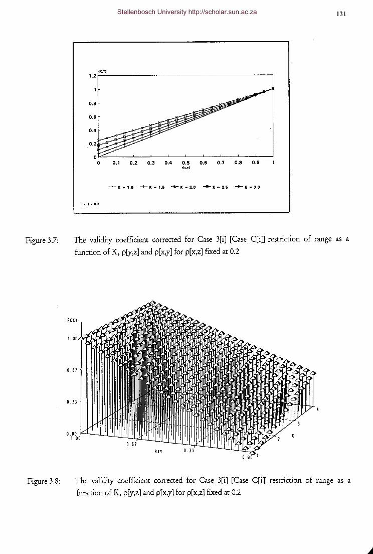
Figure 3.7:
Figure 3.8:
131
riX.YI 1.2.--------------------------,
0.8
0.6
0.4
0.2
0.1 0.2 0.3 0.4 0.5 0.6 0.7 0.8 0.9 rla.yl
- K • 1.0 -+- K • 1.5 ~ K • 2.0 -e- K • 2.5 .._ K • 3.0
r(a.z) • O.Z
The validity coefficient corrected for Case 3[i] [Case C[i] restriction of range as a
function of K, p[y,z] and p[x,y] for p[x,z] fixed at 0.2
The validity coefficient corrected for Case 3[i] [Case C[i] restriction of range as a
function of K, p[y,z] and p[x,y] for p[x,z] fixed at 0.2
Stellenbosch University http://scholar.sun.ac.za
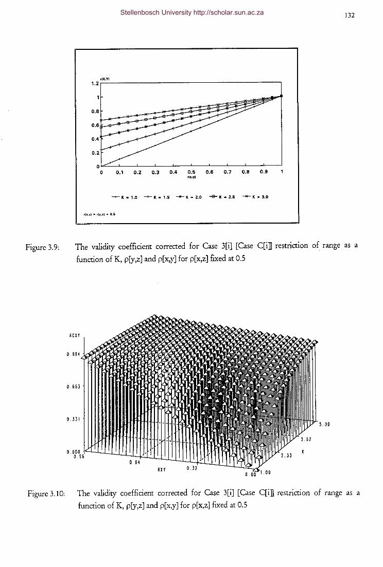
Figure 3.9:
riX.YI 1.2..------------------------,
0.4
0.1 0.2 0.3 0.4 0.5 0.6 0.7 0.8 0.9 rta.y)
-Ka1.0 --+-K-1.5 -<IE-K•2..0 -B-K•2..5 --K-3.0
rl•.zl • rly.z) • 0.&
132
The validity coefficient corrected for Case 3[i] [Case C[i] restriction of range as a
function of K, p[y,z] and p[x,y] for p[x,z] fixed at 0.5
5.00
Figure 3.10: The validity coefficient corrected for Case 3[i] [Case C[i] restriction of range as a
function of K, p[y,z] and p[x,y] for p[x,z] fixed at 0.5
Stellenbosch University http://scholar.sun.ac.za
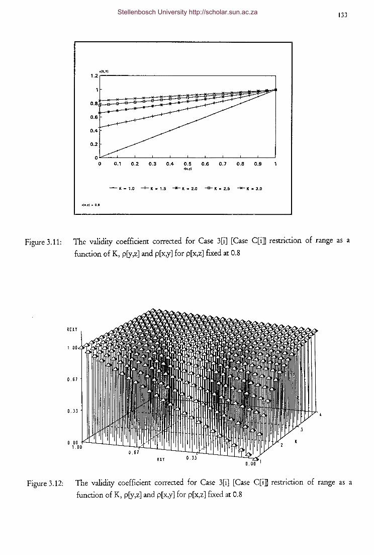
133
riX.YI 1.2,------------------------,
0.1 0.2 0.3 0.4 0.5 0.6 0. 7 0.8 0.9 rlx.y)
- K = 1.0 ~ K • 1.5 ...._. K a 2.0 -6- K E 2.5 """*- K a 3.0
rlx.zl • 0.8
Figure 3.11: The validity coefficient corrected for Case 3[i] [Case C[i] restriction of range as a
function of K, p[y,z] and p[x,y] for p[x,z] fixed at 0.8
Figure 3.12: The validity coefficient corrected for Case 3[i] [Case C[i] restriction of range as a
function of K, p[y,z] and p[x,y] for p[x,z] fixed at 0.8
Stellenbosch University http://scholar.sun.ac.za
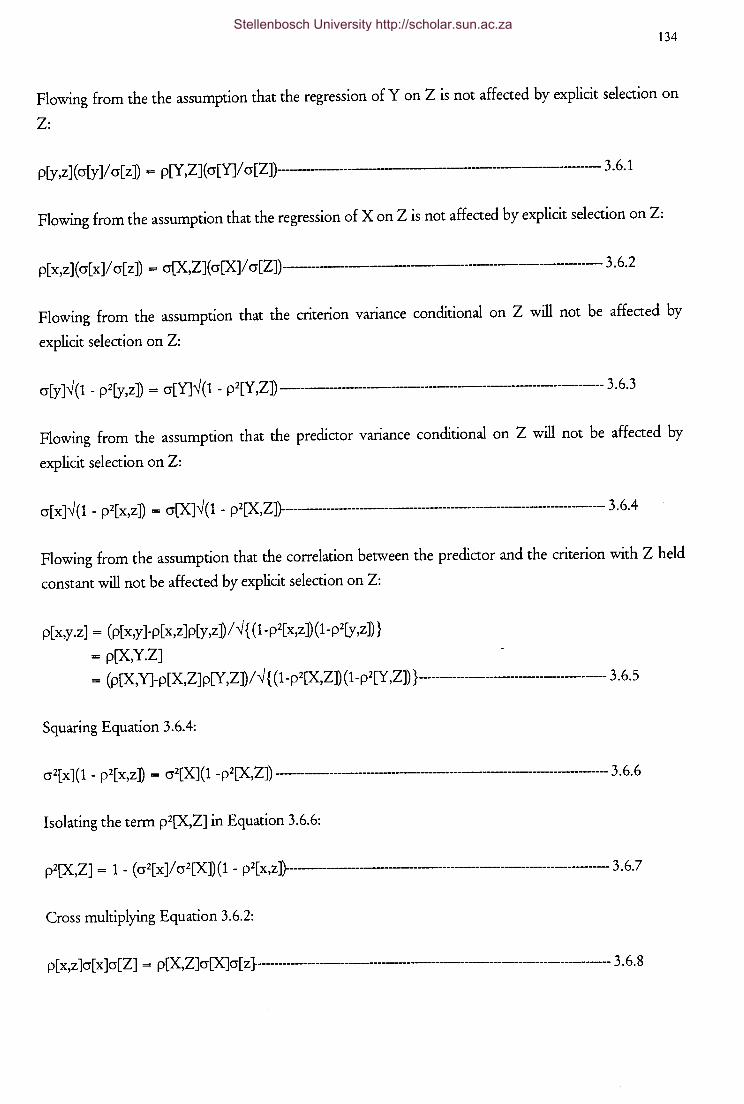
134
Flowing from the the assumption that the regression of Y on Z is not affected by explicit selection on
Z:
p[y,z ]( cr[y ]/ cr[ z ]) = p[Y,Z]( cr[Y]/ cr[Z])--------------------------------------- 3 .6.1
Flowing from the assumption that the regression of X on Z is not affected by explicit selection on Z:
p[ x,z ]( cr[x ]/ cr[ z ]) = cr[X,Z]( cr[X]/ cr[Z])------------------------------------------- 3 .6.2
Flowing from the assumption that the criterion variance conditional on Z will not be affected by
explicit selection on Z:
cr[y ]vi ( 1 - p2[y,z ]) = cr[Y]vi ( 1 - p2[Y ,Z]) ---------------------------------------------------------------- 3. 6.3
Flowing from the assumption that the predictor variance conditional on Z will not be affected by
explicit selection on Z:
cr[ x ]vi ( 1 - p2[ x,z ]) = cr[X]vi ( 1 - p2[X,Z]}-------------------------------------------------------------------------- 3. 6. 4
Flowing from the assumption that the correlation between the predictor and the criterion with Z held
constant will not be affected by explicit selection on Z:
p[x,y.z] = (p[x,y]-p[x,z]p[y,z])/vi{ (1-p2[x,z])(1-p2[y,z])}
= p[X,Y.Z]
= (p[X,Y]-p[X,Z]p[Y,Z])/ vi { ( 1-p2[X,Z]) (1-p2[Y,Z]) }------------------------------------------- 3 .6.5
Squaring Equation 3.6.4:
cr2[x](1 - p2[x,z]) = cr2[X](1 -p2[X,Z]) -------------------------------------------------------------------3.6.6
Isolating the term p2[X,Z] in Equation 3.6.6:
p2[X,Z] = 1 - ( cr2[ x ]/ cr2[X]) ( 1 - p2[ x,z ])--------------------------------------------------------------------- 3. 6.7
Cross multiplying Equation 3.6.2:
p[ x,z ]cr[x ]cr[Z] = p[X,Z]cr[X]cr[ z }-------------------------------------------------------------------------------- 3. 6. 8
Stellenbosch University http://scholar.sun.ac.za
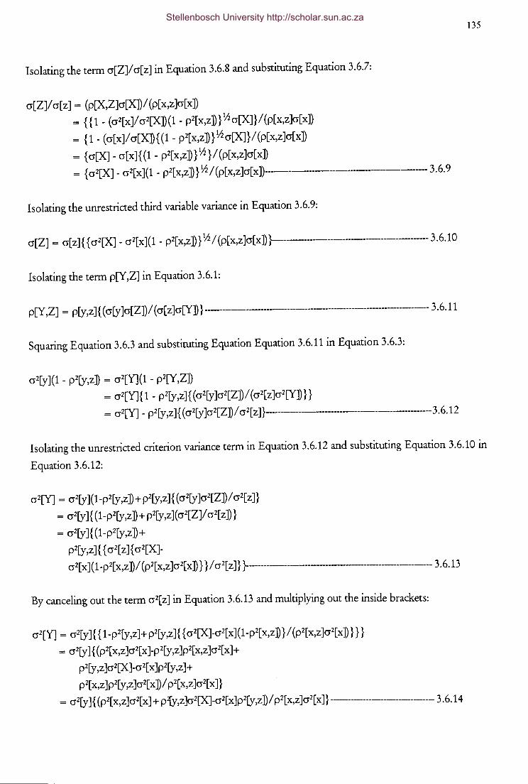
Isolating the term cr[Z]I cr[z] in Equation 3.6.8 and substituting Equation 3.6.7:
cr[Z]Icr[z] = (p[X,Z]cr[X])I(p[x,z]cr[x]) = { { 1 - ( cr2[ x ]I cr2[X]) ( 1 - p2[ x,z]} 1h cr[X]}/ (p[ x,z ]cr[ x ])
= { 1 - ( cr[ x ]I cr[X] { ( 1 - p2[ x,z ]) } 1h cr[X] }/ (p[ x,z ]cr[ x ])
= { cr[X] - cr[x ]{ ( 1 - p2[ x,z ])} 1h} I (p[ x,z ]cr[ x ]) = {cr2[X]- cr2[x](1- p2[x,z]} lhl(p[x,z]cr[x])---------------------------------------- 3.6.9
Isolating the unrestricted third variable variance in Equation 3.6.9:
cr[Z] = cr[ z] { { cr2[X] - cr2[ x ]( 1 - p2[ x,z ]) } 1h I (p[ x,z ]cr[x ]) }--------------------------------------------- 3. 6.10
Isolating the term p[Y,Z] in Equation 3.6.1:
p[Y,Z] = p[y,z] { ( cr[y ]cr[Z])I ( cr[ z ]cr[Y])} ------------------------------------------------------------------------ 3. 6.11
Squaring Equation 3.6.3 and substituting Equation Equation 3.6.11 in Equation 3.6.3:
cr2[y](1- p2[y,z]) = cr2[Y](1- p2[Y,Z])
= cr2[Y]{1- p2[y,z]{(cr2[y]cr2[Z])I(cr2[z]cr2[Y])}}
= cr2[Y] - p2[y ,z] { ( cr2 [y ]cr2[Z]) I cr 2 [ z]} -------------------------------------------------------3 . 6.12
135
Isolating the unrestricted criterion variance term in Equation 3.6.12 and substituting Equation 3.6.10 in
Equation 3.6.12:
cr2[Y] = cr2[y](1-p2[y,z])+ p2[y,z]{ (cr2[y]cr2[Z])I cr2[z]}
= cr2[y]{ (1-p2[y,z])+ p2[y,z](cr2[Z]I cr2[z])}
= cr2[y]{(1-p2[y,z])+
p2[y,z]{ { cr2[z]{ cr2[X]-cr2[ x] ( 1-p2[ x,z ]) I (p2[ x,z ]cr2[ x ]) } } I cr2[ z]} }----------------------------------------------------------- 3. 6.13
By canceling out the term cr2[z] in Equation 3.6.13 and multiplying out the inside brackets:
cr2[Y] = cr2[y]{ {1-p2[y,z]+p2[y,z]{ {cr2[X]-cr2[x](1-p2[x,z]}l(p2[x,z]cr2[x])}}}
= cr2[y] { (p2[ x,z ]cr2[ x ]-p2[y,z ]p2[ x,z ]cr2[ x ]+
p2[y,z]cr2[X]-cr2[x]p2[y,z]+
p2[ x,z] p2[y ,z ]cr2[ x ]) I p2[ x,z ]cr2[ x]}
= cr2[y ]{ (p2[ x,z ]cr2[ x] + p2(y,z ]cr2[X]-cr2[ x ]p2[y,z ])I p2[ x,z ]cr2[x ]} ---------------------------------- 3. 6.14
Stellenbosch University http://scholar.sun.ac.za
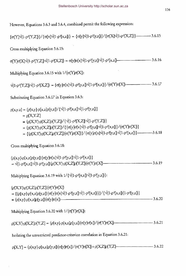
However, Equations 3.6.3 and 3.6.4, combined permit the following expression:
{ cr[Y]v'(1-p2[Y,Z]) }I { cr[x]v'(1-p2[x,z])} = { cr[y]v'(1-p2[y,z]) }/ { cr[X]v'(1-p2[X,Z]) }------------ 3.6.15
Cross multiplying Equation 3.6.15:
cr[Y]cr[X]v'(1-p2[Y,Z])v'(1-p2[X,Z]) = cr[y]cr[x]v'(1-p2[y,z]v'(1-p2[x,z]}------------------------- 3.6.16
Multiplying Equation 3.6.15 with 11(cr[Y]cr[X]):
v'(1-p2[Y,Z])v'(1-p2[X,Z]) = { cr[y ]cr[x]v'(1-p2[y,z])v'(1-p2[x,z])} I (cr[Y]cr[X]}------------------------ 3.6.17
Substituting Equation 3.6.17 in Equation 3.6.5:
p[x,y.z] = (p[x,y]-p[x,z]p[y,z])l { v'(1-p2[x,z])v'(1-p2[y,z])}
= p[X,Y.Z]
= (p[X,Y]-p[X,Z]p[Y,Z])I { v' ( 1-p2[X,Z]) v' (1-p2[Y,Z])}
= (p[X,Y]-p[X,Z]p[Y ,Z]) I { { cr[y ]cr[ x ]v' ( 1-p2[y,z ]) v' ( 1-p2[ x,z ]) } I ( cr[Y]cr[X]}
= { (p[X,Y]-p[X,Z]p[Y,Z])(cr[Y]cr[X]) }/ { cr[y]cr[x]v'(1-p2[y,z])v'(1-p2[x,z]) }---------------3.6.18
Cross multiplying Equation 3.6.18:
(p[x,y]-p[x,z]p[y,z] { cr[y ]cr[x]v'(1-p2[y,z])v'(1-p2[x,z])}
= v'(1-p2[x,z])v'(1-p2[y,z])(p[X,Y]-p[X,Z]p[Y,Z])( cr[Y]cr[X]--------------------------------------------- 3.6.19
Multiplying Equation 3.6.19 with 11 { v'(1-p2[x,z])v'(1-p2[y,z]) }:
(p[X,Y]-p[X,Z]p[Y ,Z]) ( cr[Y]cr[X])
= { (p[x,y]-p[x,z]p[y,z]) { cr[y]cr[x]v'(1-p2[y,z])v'(1-p2[x,z])} }I { v'(1-p2[x,z])(1-p2[y,z])}
= (p[ x,y ]-p[ x,z ]p[y,z ]) ( cr[y ]cr[ x ]}--------------------------------------------------------------------------- 3 .6.20
Multiplying Equation 3.6.20 with 1l(cr[Y]cr[X]):
p[X,Y]-p[X,Z]p[Y ,Z] = (p[ x,y ]-p[ x,z ]p[y,z ]) ( cr[y ]cr[ x ])I ( cr[Y]cr[X]}---------------------------------- 3. 6.21
Isolating the unrestricted predictor-criterion correlation in Equation 3.6.21:
p[X, Y] = (p[ x,y ]-p[ x,z] p[y ,z ]) ( cr[y ]cr[ x ]) I ( cr[Y]cr[X]) + p[X,Z] p[Y,Z}---------------------------------- 3. 6.22
136 Stellenbosch University http://scholar.sun.ac.za

From Equations 3.6.1 and 3.6.2 it follows that:
{p[y,z](cr[y]l cr[z]) }/ {p[X,Z](cr[X]I cr[Z])} = {p[Y,Z](cr[Y]I cr[Z]) }/ {p[x,z](cr[x]l cr[z] }----- 3.6.23
Cross multiplying Equation 3.6.23:
{p[X,Z](cr[X]I cr[Z])} {p[Y,Z](cr[Y]I cr[Z])} = {p[y,z](cr[y]l cr[z]} {p[x,z](cr[x]l cr[z]}
= p[y ,z]p[x,z]{ (cr[y]cr[x])l (cr[z]cr[z])}--------------- 3.6.24
Therefore:
p[X,Z]p[Y,Z]{ (cr[X]cr[Y])I cr2[Z]} = p[y,z]p[x,z]{ (cr[y]cr[x])l cr2[z]}------------------------------ 3.6.25
Multiplying Equation 3.6.25 with cr2[Z]I(cr[X]cr[Y])
p[X,Z]p[Y ,Z] = p[y,z ]p[ x,z] { ( cr[y ]cr[ x ]cr2[Z]) I ( cr2[ z ]cr[X]cr[Y]) }---------------------------------------- 3. 6.26
Substituting Equation 3.6.26 in Equation 3.6.22:
p[X,Y] = { (p[x,y ]-p[ x,z]p[y,z ]) ( cr[y ]cr[ x ])I ( cr[Y]cr[X])} +
p[y,z ]p[ x,z] { ( cr[y ]cr[ x ]cr2(Z]) I ( cr2[ z ]cr[X]cr[Y]}
= { ( cr[y ]cr[ x ]) I ( cr[Y]cr[X]) }(p[ x,y ]-p[x,z ]p[y,z ]) +
p [y ,z] p[ x,z] ( cr2 [Z]I cr2[ z ]) --------------------------------------------------------------------------------- 3 . 6. 27
Substituting for cr[Y] and cr[Z] in Equation 3.6.27 through Equations 3.6.14 and 3.6.10:
p[X,Y] = (cr[y]cr[x])l { {cr[y]{(p2[x,z]cr2[x]+
p2[y,z]cr2[X]-cr2[x]p2[y,z]) ~I p[x,z]cr[x]} }cr[X]} {p[x,y]-p[x,z]p[y,z]} +
p[y,z]p[x,z]({ cr[z]{ { cr2[X]-cr2[x](1-p2[x,z])} ~I p[x,z]cr[x]}} I cr2[z])}
= {p[x,z]cr2[x]p[x,y]+p[y,z](cr2[X]-cr2[x]) }I { cr[X](p2[x,z]cr2[x]+
p2[y,z] ( cr2[X]-cr2[ x ]) ) ~ } --------------------- ----------------------------- 3. 6
137
Case C, in which restriction is indirect, imposed by explicit selection on a third [single or composite]
variable, seems to be the most common and most important case in personnel validation research.
Restriction of range through systematic selection reduces the magnitude of the correlation estimate,
sometimes to such an extent that the sign of the correlation calculated for the selected group differs in
sign from that applicable to the unrestricted group [Linn, 1983; Ree, Carretta, Earles & Albert, 1994].
Stellenbosch University http://scholar.sun.ac.za
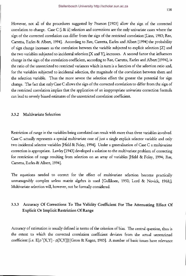
138
However, not all of the procedures suggested by Pearson [1903] allow the sign of the corrected
correlation to change. Case C [i & ii] selection and corrections are the only univariate cases where the
sign of the corrected correlation can differ from the sign of the restricted correlation [Linn, 1983; Ree,
Carretta, Earles & Albert, 1994]. According to Ree, Carretta, Earles and Albert [1994] the probability
of sign change increases as the correlation between the variable subjected to explicit selection [Z] and
the two variables subjected to incidental selection [X and Y], increases. A second factor that influences
change in the sign of the correlation coefficient, according to Ree, Carretta, Earles and Albert [1994], is
the ratio of the unrestricted to restricted variances which in tum is a function of the selection ratio and,
for the variables subjected to incidental selection, the magnitude of the correlation between them and
the selection variable. Thus the more severe the selection effect the greater the potential for sign
change. The fact that only Case C allows the sign of the corrected correlation to differ from the sign of
the restricted correlation implies that the application of an inappropriate univariate correction formula
can lead to severly biased estimates of the unrestricted correlation coefficient.
3.3.2 Multivariate Selection
Restriction of range in the variables being correlated can result with more than three variables involved.
Case C actually represents a special multivariate case of just a single explicit selector variable and only
two incidental selector variables [Held & Foley, 1994]. Under a generalisation of Case C a multivariate
correction is appropriate. Lawley [1943] developed a solution to the multivariate problem of correcting
for restriction of range resulting from selection on an array of variables [Held & Foley, 1994; Ree,
Carretta, Earles & Albert, 1994].
The equations needed to correct for the effect of multivariate selection become practically
unmanageably complex unless matrix algebra is used [Gulliksen, 1950; Lord & Novick, 1968;].
Multivariate selection will, however, not be formally considered.
3.3.3 Accuracy Of Corrections To The Validity Coefficient For The Attenuating Effect Of
Explicit Or Implicit Restriction Of Range
Accuracy of estimation is usually defined in terms of the criterion of bias. The central question, thus is
the extent to which the corrected correlation coefficient deviates from the actual unrestricted
coefficient [i.e. E[pA[X,Y]- p[X,Y]]] [Gross & Kagen, 1983]. A number of basic issues have relevance
Stellenbosch University http://scholar.sun.ac.za
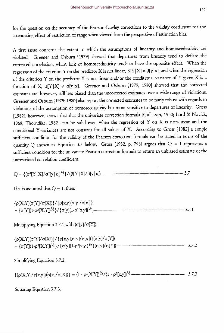
139
for the question on the accuracy of the Pearson-Lawley corrections to the validity coefficient for the
attenuating effect of restriction of range when viewed from the perspective of estimation bias.
A first issue concerns the extent to which the assumptions of linearity and homoscedasticity are
violated. Greener and Osburn [1979] showed that departures from linearity tend to deflate the
corrected correlation, whilst lack of homoscedasticity tends to have the opposite effect. When the
regression of the criterion Yon the predictor X is not linear, p[YIXJ * p[ylxJ, and when the regression
of the criterion Y on the predictor X is not linear and/ or the conditional variance of Y given X is a
function of X, cr[YIXJ * cr[ylxJ. Greener and Osburn [1979; 1980] showed that the corrected
estimates are, however, still less biased than the uncorrected estimates over a wide range of violations.
Greener and Osburn [ 1979; 19 80] also report the corrected estimates to be fairly robust with regards to
violations of the assumption of homoscedasticity but more sensitive to departures of linearity. Gross
[1982], however, shows that that the univariate correction formula [Gulliksen, 1950; Lord & Novick,
1968; Thorndike, 1982] can be valid even when the regression of Y on X is non-linear and the
conditional Y-variances are not constant for all values of X. According to Gross [1982] a simple
sufficient condition for the validity of the Pearson correction formula can be stated in terms of the
quantity Q shown as Equation 3.7 below. Gross [1982, p. 798] argues that Q = 1 represents a
sufficient condition for the univariate Pearson correction formula to return an unbiased estimate of the
unrestricted correlation coefficient:
Q = { ( cr2[Y I X]/ cr2[y I x ]) Y2} I (p[Y I X]/ P[y I x ]) ------------------------------------------------------------- 3.7
If it is assumed that Q = 1, then:
{ p[X,Y]( cr[YJ/ cr[X])} I { p[ x,y ]( cr[y ]/ cr[ x ]) }
= { cr[Y] ( 1-p2[X, Y]) Y2 } I { cr[y ]( 1-p2[ x,y ]) Y2 }----------------------------------------------------- 3. 7.1
Multiplying Equation 3.7.1 with (cr[y]/cr[YJ):
{ p[X, Y] ( cr[YJ/ cr[X]) } I { p[ x,y ]( cr[y ]/ cr[ x ]) }( cr[y ]/ cr[Y])
= { cr[Y](1-p2[X,Y]) Y2 }/ { cr[y ](1-p2[x,y]) Y2 }( cr[y ]/ cr[Y])----------------------------------~---------- 3.7.2
Simplifying Equation 3.7.2:
{(p[X,Y]/p[x,y])(cr[x]/cr[X]} = (1- p2[X,YJ)Yl/(1- p2(x,y])Yl--------------------------------- 3.7.3
Squaring Equation 3.7.3:
Stellenbosch University http://scholar.sun.ac.za
140
{ (p2[X, Y]l p2[ x,y ]) ( cr2[ x ]I cr2[XJ) } = ( 1 - p2[X,Y]) I ( 1 - p2[ x,y ]) ------------------------------------- 3. 7. 4
Subtracting { (p2[X,Y]I p2[x,y])(cr2[x]l cr2[X])} on both sides of Equation 3.7.4:
(1 - p2[X,Y])I (1-p2[x,y] - { (p2[X,Y]I p2[x,y])(cr2[x]l cr2[X])} = 0--------------------------------- 3.7.5
Multiplying Equation 3.7.5 with (1-p2[x,y]:
(1 - p2[X,Y]) - (1 - p2[x,y]){ (p2[X,Y]I p2[x,y])(cr2[x]l cr2[X])} = 0.------------------------------------- 3.7.6
Multiplying Equation 3.7.6 with (-1):
(-1){ (1-p2[X,Y]) - (1 - p2[x,y]){ (p2[X,Y]I p2[x,y ])(cr2[x]l cr2[X])}} = 0.--------------------------------- 3.7.7
Therefore:
p2[X,Y] + ( 1 - p2[ x,y ]) { (p2[X,Y]I p2[ x,y ]) ( cr2[ x ]I cr2[X])} = 1----------------------------------------------- 3.7. 8
By factoring out the term p2[X,Y] in Equation 3.7.8:
p2[X,Y] { 1 + ( 1 - p2[ x,y] ( cr2[ x ]I (p2[ x,y ]cr2[X]))} = 1----------------------------------------------------------- 3.7. 9
Placing the term {1 + (1- p2[x,y](cr2[x]l(p2[x,y]cr2[X]))} in Equation 3.7.9 on a common denominator:
p2[X, Y] { (p2[ x,y Jcr2[XJ + ( 1 - p2[ x,y ]) cr2[ x ]) I (p2[x,y ]cr2[X]) } = 1------------------------------------------- 3 .7 .1 0
Therefore:
p2[X,Y] { (p2[ x,y] + ( 1 - p2[ x,y ]) ( cr2[ x ]I cr2[X])) I p2[x,y]} = 1----------------------------------------------- 3.7 .11
Cross multiplying Equation 3.7.11 and isolating the term p2[X,Y]:
p2[X,Y] = p2[ x,y ]I { p2[ x,y] + ( 1 - p2[ x,y ]) ( cr2[ x ]I cr2[X])} -------------------------------------------------- 3.7 .12
Taking the square root of Equation 3.7.12:
p[X,Y] = p[x,y]l{p2[x,y] + (1- p2[x,y])(cr2[x]lcr2[X])}lh
=Equation 3.4 if Q = 1
Stellenbosch University http://scholar.sun.ac.za
141
The traditional linearity and homoscedasticity assumptions thus represent only a special case where Q
= 1 and consequently where the correction formula value equals p[X,Y] [Gross, 1982; Held & Foley,
1992]. However, the condition Q = 1 may still hold even if the regression is non-linear and
heteroscedastic, although not necessarily for all selection [i.e. restriction] procedures [Gross, 1982].
Conversely, assuming p[Y I X] and P[y I x] are positive, the condition Q > 1 would imply that the
correction formula will overestimate the unrestricted correlation coefficient, whereas Q < 1 would
imply an underestimation of the unrestricted correlation coefficient [i.e. the validity coefficient
pertaining to the unselected applicant population] [Gross, 1982; Held & Foley, 1992; Schepers, 1996].
The condition Q > 1 [i.e. the corrected value shows a positive bias] will result only when the regression
of Y on X is non-linear and heteroscedastic in the unrestricted group, and selection occurs such that
the restricted group has a steeper slope and smaller cr[ylxJ than the unrestricted group. Campbell
[ 1991] maintains that the conditions under which this would happen are unlikely to be encountered in
practice. Holmes [1990] contends that overestimation will occur only when the ratio of the standard
error of prediction at the mean is at least three times as great as at the upper extreme and the selection
ratio is 0,40 or less. Again, such a diamond-shaped bivariate scatterplot seems highly improbable
[Campbell, 1991]. Schepers [1996] views Gross' Q-coeffisient as an important contribution of great
practical value and recommends its routine application whenever corrections for restriction of range are
made. Obtaining all the relevant data to calculate Q might, however, often present an insurmountable
obstacle to the implementation of this recommendation.
A second issue concerns the extent to which all the variables on which selection was based are in fact
acknowledged as explicit selection variables in the correction formula. In essence the question is thus
whether the chosen formula provides an adequate model of the selection process. Quite often the
reality of the selection process is not as neat and simple to fit into one of the categories of the
Thorndike [1949; 1982] taxonomy. The most important problem seems to be that selection in reality
most probably would have been based partly [i.e. in addition to an objectively measured single or
composite selection variable] or totally on a number of unspecified variables combined in an
unspecifiable way [i.e. clinically combining clinical judgements]. Consequently, and contrary to Case 1
[Case B] and Case 2 [Case A] assumptions, incomplete truncation on the selection variable occur [Olsen
& Becker, 1983]. The real problem, however, lies in the fact that measurements of the true explicit
selection variables are not accessible and consequently, the Pearson-Lawley correction formula
presented thus far, offer no solution to the problem. Thorndike [1949, p. 176] expresses the dilemma
experienced by the preceding, traditional correction formula as follows:
[The aforementioned situation] represents an insuperable obstacle to any analytical treatment. When
selection is based, as it often is, on clinical judgement which combines in an unspecified and inconstant
fashion various types of data about the applicant, and when this judgement is not expressed in any type of
Stellenbosch University http://scholar.sun.ac.za
quantitative score, one is at a loss as how to estimate the extent to which the validity coefficient for any test
procedure has been affected by that screening.
142
According to Campbell [1991] selection on variables not accounted for by the chosen correct10n
formula will bias the correction in ways that are at this point in time not altogether predictable. At the
same time, however, Campbell [1991] maintains that selection on variables not accounted for in the
correction formula never produces positive bias in the corrected coefficient. Levine [1972] and
McGuire [1986] contend that the corrected estimate might actually be lower than the uncorrected
correlation coefficient if the unknown selection variable is a very strong suppressor variable [i.e. highly
correlated with X but uncorrelated with Y] or the distributions are extremely leptokurtic. The
probability of these radical conditions actually being encountered are, however, extremely remote
[Campbell, 1991; Levine, 1972; McGuire, 1986]. Treating an incidental selection variable as if it were
an explicit selection variable typically results in a too conservative correction [Lord & Novick, 1968].
Lord and Novick [1968, p. 148] furthermore suggest a quasi-experimental approach to alleviate the
problem of poor model fit.
It is necessary to isolate an explicit selection variable. This can often be done by arranging for the selection
of all applicants whose test score is above some specified value. Applicants whose scores are below this value
can also be selected as desirable, but for statistical calculations these applicants are not considered part of the
selected group. This compromise arrangement should prove acceptable, administratively, in many situations.
A third issue concerns the extent to which selection has taken place. Lord and Novick [1968, p. 148]
discourage the application of the correction formulas when extreme selection has occured on the
grounds that the accuracy of the formulas decreace as the selection ratio increases.
Caution must be used to ensure that formulas are not applied when extreme selection has taken place. It is
quite clear that the accuracy of the formulas decreases as the selection ratio increases.
A fifth issue concerns the magnitude of the uncorrected validity coefficient. Greener and Osburn
[1979] found corrected validities to be less accurate than uncorrected validities at the low range of the
validity scale. Corrected correlation coefficients in general tend to be more accurate estimators than the
uncorrected ones for moderate to large unrestricted population correlations [Greener & Osburn, 1979;
Mendoza, Hart & Powell, 1991].
Campbell [1991, pp. 696-697], arguing from an estimation bias perspective, summerises the literature
on the accuracy of the traditional Pearson-Thorndike restriction of range corrections as follows:
Stellenbosch University http://scholar.sun.ac.za
Based on the above literature, there seems little reason to avoid using corrections for restriction of range.
Their shortcomings are not that they cany a large risk of overestimating the population value, but that they
still yield large underestimates under a variety of realistic conditions.
143
Gross and Kagen [1983], and Greener and Osburn [1979], however, in contrast to Campbell [1991],
maintain that corrections for restriction of range are not always advantageous. This apparent
contradiction originates in differences in the operationalisation of the term accuracy. Instead of
approaching accuracy from the perspective of the expected deviation of the [uncorrected or corrected]
sample estimate from the actual population value [i.e. E[pA[X,Y] - p[X,Y]], Gross and Kagen [1983]
argue in favour of the expected mean square error [EMSE] [i.e. E[p A[X,Y] - p[X,Y]]2 as a criterion of
estunat10n accuracy. Gross and Kagen [1983, pp. 390-391] present the essence of their argument as
follows:
It can be argued that EMSE represents a more meaningful criterion of the accuracy of estimation than the
criterion of bias. The basis for the argument is that the EMSE criterion reflects not only the bias of an
estimator, but also its sampling variance. .... More specifically for small sample sizes, and small Pxy values,
the EMSE value for r a can be substantially smaller than that for the corrected correlation [ r cJ. Thus, it can be
advantageous to estimate the population correlation using the uncorrected correlation [raJ rather than the
corrected correlation [rcJ.
The Gross and Kagen [1983] commentary should not be taken to mean that the Pearson-Thorndike
corrections should not be applied. The conditions under which the uncorrected coefficient would
result in a smaller EMSE are limited to a weak p[X,Y] relationship, extreme selection and small selected
groups; the majority of situations would still favour the application of the correction formula.
3.4 THE VALIDITY COEFFICIENT CORRECTED FOR THE JOINT
ATTENUATING EFFECT OF EXPLICIT OR IMPLICIT RESTRICTION OF
RANGE AND THE UNRELIABILITY OF THE CRITERION MEASUREMENTS
Although considerable literature eXIsts regarding the correct10n of correlation coefficients for the
seperate attenuating effects of measurement error and restriction of range [Ghiselli, Campbell &
Zedeck, 1981; Gulliksen, 1950; Held & Foley, 1994; Linn, 1983; Olson & Becker, 1983; Pearson, 1903;
Ree, Carretta, Earles & Albert, 1994 ], relatively little attention has been given to the theory underlying
the correction of a correlation coefficient for the joint effects of measurement error and restriction of
Stellenbosch University http://scholar.sun.ac.za
144
range [Bobko, 1983; Lee, Millar & Graham, 1982; Mendoza & Mumford, 1987; Schmidt, Hunter &
Uny, 1976].
In a typical validation study, restriction of range and criterion unreliability are simultaneously present.
Their effects combine to yield an attenuated validity coefficient that could severely underestimate the
operational validity [Lee, Millar & Graham, 1982; Schmidt, Hunter & Uny, 1976]. It thus seems to
make intuitive sense to double correct an obtained validity coefficient for the attenuating affect of both
factors. The APA, however, through their Standards for Educational and Psychological Tests [APA,
1974, p.41], initially recommended that:
It is ordinarily unwise to make sequential corrections, as in applying a correction for attenuation to a
coefficient already corrected for restriction of range. Chains of corrections may be useful in considering
possible further research, but their results should not be seriously reported as estimates of population
correlation coefficients.
Schmidt, Hunter and Uny [1976], though, consider the APA recommendation to be in error and
propose that the obtained validity coefficient should be sequentially corrected for the effects of both
restriction of range and criterion unreliability so as to obtain an estimate of the actual operational
validity. The revised edition of the Standards for Educational and Psychological Tests [APA, 1985]
subsequently also seems to have softened is position on this topic by abstaining from any comment.
The stepwise correction procedure suggested by Schmidt, Hunter and Uny [1976] involves first
correcting both the obtained validity and reliability coefficients for restriction of range since both
coefficients apply only to a restricted applicant group and thus are to a greater or lesser extent
negatively biased estimates of the operational reliability and validity coefficients. Equation 3.8 is
suggested as an appropriate correction formula to correct the reliability coefficient for the attenuating
affect of restriction of range if homogeneity of error variance across values of the range of true
criterion scores can be assumed [i.e. the assumption is that applicants were selected in such a manner
that the true score variance reduces whereas the error variance remains unaffected] [Feldt & Brennan,
1989; Ghiselli, Campbell & Zedeck, 1981; Guion, 1965; Gulliksen, 1950; Lee, Millar & Graham, 1982].
From the assumption of homogeneous error variance across values of the range of true criterion scores
it follows that:
cr[y ]vi ( 1 - Ptty) = cr[Y]v' ( 1 - Ptt y) ------------------------------------------------------------------------ 3. 8 .1
Squaring Equation 3.8.1:
cr2[y] ( 1 - Ptty) = cr2[Y] ( 1 - Ptt y) --------------------------------------------------------------------------- 3. 8.2
Stellenbosch University http://scholar.sun.ac.za
145
Multiplying Equation 3.8.2 by 1/ cr2[Y]:
(cr2[y]/cr2[Y])(1- Ptty) = (1- PttY)---------------------------------------------- 3.8.3
Isolating the unrestricted reliability coefficient in Equation 3.8.3:
Ptt y = 1 - { ( cr[y ]/ cr[Y])2(1 - Pny)}- --------------------- 3.8
The assumption Equation 3.8 is based on, however, frequently does not hold [Feldt & Brennan, 1989].
A further problem with Equation 3.8 in the context of validation research, however, is that the criterion
variance for the unrestricted group is logically impossible to obtain.
Schmidt, Hunter and Uny [1976] suggest an alternative expression [shown as Equation 3.9] which
avoids the aforementioned problem.
Ptt y = [ 1 - [ ( 1-Pny) I ( 1-p[ x,y ]( 1-( cr2[X]/ cr2[ x ]) )-------------------------------------------------------------- 3. 9
Depending on the nature of the selection and the variable for which both the restricted and
unrestricted variance is known, the correction of the validity coefficient for the attenuating effect of
restriction of range will proceed through the appropriate correction formula taken from Equations 3.3-
3.6. The validity coefficient corrected for restriction of range will then subsequently be corrected for
the attenuation effect of criterion unreliability by employing the results of the preceding first two steps
[i.e. the reliability and validity coefficients corrected for restriction of range] in the traditional attenuation
correction formula for the criterion only [Equation 3 .2].
Lee, Miller and Graham [1982], however, point out that statistical and measurement theory permits a
simpler two-step correction. According to the Lee, Miller and Graham [1982] approach the restricted
criterion reliability coefficient is used to correct the restricted validity coefficient for the attenuating
effect due to the unreliability of the criterion. This reliability attenuation-corrected validity coefficient is
then subsequently corrected for the attenuating affect of restriction of range. The first step in the
Schmidt, Hunter and Uny [1976] procedure is thus disposed of. Although the procedures suggested by
Schmidt, Hunter and Uny [1976] and Lee, Miller and Graham [1982] seem to be conceptually distinct,
Bobko [1983] points out that these two procedures are in fact arithmetically identical. Combining the
two step-approach suggested by Lee, Miller and Graham [1982] into a single equation results in
Equation 3.10 for the double-corrected validity coefficient [assuming Case 2 [Case A] selection
produced the restriction of range] [Bobko, 1983].
p[X,Ty] = cr[X]p[x,y]p[y,yjlh/ { cr2[X]p2[x,y]p[y,y]-1 +cr2[x}cr2[x]p2[x,y]p[y,y]-1} lh _____________ 3.10
Stellenbosch University http://scholar.sun.ac.za
146
Similar equations could be derived for the other possible conditions under which correlation estimation
bias due to systematic selection could occur.
Mendoza & Mumford [1987] proposed a set of equations in terms of which correlation coefficients can
be jointly corrected for: ~ restriction of range directly on the predictor and unreliability in the predictor and
the criterion; or
~ restrictiort of range directly on the latent trait measured by the predictor and
unreliability in the predictor and the criterion
Equation 3.11 shows the appropriate correction formula applicable when restriction of range occurs
directly on the ability/latent trait measured by the predictor [Mendoza & Mumford, 1987]. The
derivation of Equation 3.11 assumes a linear, homoscedastic regression of the criterion Y on the
predictor X in the unrestricted population and in addition makes the two usual restriction of range
assumptions that: ~ the regression of actual job performance [i.e. the ultimate criterion] Y' on ability will
not be affected by explicit selection on the latent trait represented by X'; and
~ the ulimate criterion variance conditional on X' will not be altered by explicit
selection on the latent trait measured by X [Mendoza & Mumford, 1987].
From the assumption that the regression of actual job performance [i.e. the ultimate criterion] Y' on
ability will not be affected by explicit selection on the latent trait represented by X, it follows that:
p[ 1).1 tJ = p[T y IT xJ ------------------------------------------------------------------------------------------------- 3 .11.1
From the assumption that the ulimate criterion variance conditional on X' will not be altered by explicit
selection on the latent trait measured by X, it follows that:
cr2[ty](1 - p2[txty]) = cr2[T y](1 - p2[T x,Ty] --------------------------------------------------- 3.11.2
However
pz[ s.l tJ = p2[ tytx]( cr2[ ty ]/ cr2[ txD = p2[ tytxH ( cr2[y ]Ptty) I ( cr2[ x ]pnx)} ----------------------------------------------------------- 3 .11. 3
Similarly:
Stellenbosch University http://scholar.sun.ac.za
147
= pz[fyTx]{ (cr2[Y]puy)/(cr2[X]pttX)} -------------------------------3.11.4
Substituting Equations 3.11.3 and 3.11.4 in Equation 3.11.1:
Isolating the term p2[fyTxJ in Equation 3.11.5 by multiplying by {(cr2[X]pttX)/(cr2[YJPttY)}
pz[fyTxJ = p2[tytx]{ (cr2[y]Puy)l(cr2[x]pux) }{ (cr2[XJpttX)/(cr2[Y]ptty)}
= p2[ tytx] { cr2[y Jpuycr2[X] PttX} I { cr2[ x ]Pttxcr2[Y]Ptt y} ------------------------------ 3 .11. 6
However, according to Equation 3.1:
p2[ t}y] = p2[ x,y ]/ (PttxPtty) ------------------------------------------------------------------------------------------- 3 .11.7
Substituting Equation 3 .11.7 in Equation 3 .11. 6:
P2[T x,Ty] = {p2[x,y]/ (PttxPtty) }{ cr2[y]puycr2[X]pttX}/ { cr2[x]Pttxcr2[Y]PuY}
= (p2( x,y ]crZ(y ]cr2[X]pttX)/ ( crz[ x ]Pzttxcrz[Y]puy}------------------------------- 3.11
Equation 3.11 places rather formidable demands in as far as it requires the reliability and variance of
both variables in both the restricted and unrestricted groups to be known. This seems to limit the
practical value of Equation 3.11. If it is possible to calculate both cr2[X] and cr2[Y] [and not only one of
the two], it seems more than probable that one would also be able to calculate p[X,Y], PttX ardPttY
and thus estimate p[fx,Ty] with the traditional attenuation correction formula [Equation 3.1]. The
need to infer p[Tx,Ty] indirectly via an equation like Equation 3.11, would then no longer exists.
Mendoza and Mumford [1987] acknowledge the equation's requirement that the reliability of both
measures be known in in the restricted and unrestricted space, but do not regard this as a problem since
the restricted and unrestricted reliabilities are related by Equation 3.8.
Equation 3.12 applies to the second, probably more prevalent, s1tuat10n where restnct10n of
range/ selection occurs directly on the predictor [Mendoza & Mumford, 1987]. The derivation of
Equation 3.12 assumes a linear, homoscedastic regression of the criterion Yon the predictor X in the
unrestricted population and in addition makes the two usual restriction of range assumptions that:
~ the regression of the criterion Y on the predictor will not be affected by explicit
selection on the predictor X; and
~ the criterion variance conditional on X will not be altered by explicit selection on X
[Mendoza & Mumford, 1987].
Stellenbosch University http://scholar.sun.ac.za
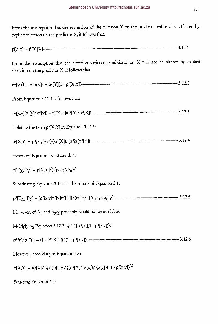
148
From the assumption that the regression of the criterion Y on the predictor will not be affected by
explicit selection on the predictor X, it follows that:
p[y I X] = p[Y I X]------------------------------------------------------------------------------------ 3 .12.1
From the assumption that the criterion variance conditional on X will not be altered by explicit
selection on the predictor X, it follows that:
cr2[y] ( 1 - p2 [ x,y ]) = cr2[Y] ( 1 - p2[X,Y])------------------------------------------------------------------------- 3 .12.2
From Equation 3.12.1 it follows that:
p2[x,y ]( cr2[y ]I cr2[ x ]) = p2[X,Y]( cr2[Y]I cr2[X])---------------------------------------------------------------------- 3 .12.3
Isolating the term p2[X,Y] in Equation 3.12.3:
p2[X, Y] = p2[ x,y] ( cr2[y ]cr2[X]) I ( cr2[ x ]cr2[Y]) ---------------------------------------------------------------------- 3 .12. 4
However, Equation 3.1 states that:
Substituting Equation 3.12.4 in the square of Equation 3.1:
p2[T x, T y] = (p2[ x,y ]cr2[y ]cr2[X] I ( cr2[ x ]cr2[Y]PttXPtt y )---------------------------------------------------- 3 .12.5
However, cr2[Y] and PttY probably would not be available.
Multiplying Equation 3.12.2 by 11{cr2[Y](1- p2[x,y])}:
cr2[y ]I cr2[Y] = ( 1 - p2[X,Y]) I ( 1 - p2[ x,y ])-------------------------------------------------------------------------- 3 .12. 6
However, according to Equation 3.4:
p[X,Y] = (cr[X]Icr[x])p[x,y]l{(cr2[X]Icr2[x])p2[x,y] + 1- pl[x,y]}lh
Squaring Equarion 3.4:
Stellenbosch University http://scholar.sun.ac.za
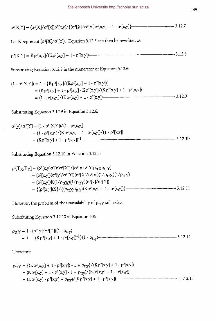
p2[X,Y] = (cr2[X]Icr2[x])p2[x,y]l{(cr2[X]Icr2[x])p2[x,y] + 1- p2[x,y]}--,---------3.12.7
Let K represent (cr2[X]Icr2[x]). Equation 3.12.7 can then be rewritten as:
p2[X,Y] = Kp2[x,y]I(Kp2[x,y] + 1- p2[x,y])----------------------------------------3.12.8
Substituting Equation 3.12.8 in the numerator of Equation 3.12.6:
(1- p2[X,Y]) = 1- {Kp2[x,y]I(Kp2[x,y] + 1- p2[x,y]}
= (Kp2[x,y] + 1- p2[x,y]- Kp2[x,y])I(Kp2[x,y] + 1- p2[x,y]
= (1 - p2[x,y]I(Kp2[x,y] + 1- p2[x,y])------------------------------------- 3.12.9
Substituting Equation 3.12.9 in Equation 3.12.6:
cr2[y ]I cr2[Y] = ( 1 - p2[X,Y])I ( 1 - p2[ x,y ])
= (1 - p2[x,y])I(Kp2[x,y] + 1 - p2[x,y])l(1 - p2[x,y]
= (Kp2[x,y] + 1 - p2[x,y ]) -1__-------------------------------------------------------------------- 3 .12.1 0
Substituting Equation 3.12.10 in Equation 3.12.5:
p2[T x, Ty] = (p2[ x,y ]cr2[y ]cr2[X])I ( cr2[ x ]cr2[Y]PttXPtt y)
= (p2[x,y ]( cr2[y ]I cr2[Y]) ( cr2[X]I cr2[ x ]) (11 PtOO ( 11 PttY)
= (p2[ x,y ]) K ( 1 I pttX) ( 1 I Ptt y) ( cr2[y ]I cr2[Y])
= { (p2[x,y])K} I { (PttXPttY) (Kp2[x,y] + 1 - p2[x,y])} ---------------------------------------- 3.12.11
However, the problem of the unavailability of PttY still exists.
Substituting Equation 3.12.10 in Equation 3.8:
PttY = 1- (cr2[y]lcr2[Y])(1- Ptty) . = 1- {(Kp2[x,y] + 1- p2[x,y]-1}(1- Ptty)-------------------------------------------------3.12.12
Therefore:
PttY = {(Kp2[x,y] + 1- p2[x,y]- 1 + Ptty}/(Kp2[x,y] + 1- p2[x,y])
= (Kp2[x,y] + 1- p2[x,y]- 1 + Ptty)I(Kp2[x,y] + 1- p2[x,y])
149
= (Kp2[x,y]- p2[x,y] + Ptty)I(Kp2[x,y] + 1- p2[x,y])---------------------------------------- 3.12.13
Stellenbosch University http://scholar.sun.ac.za
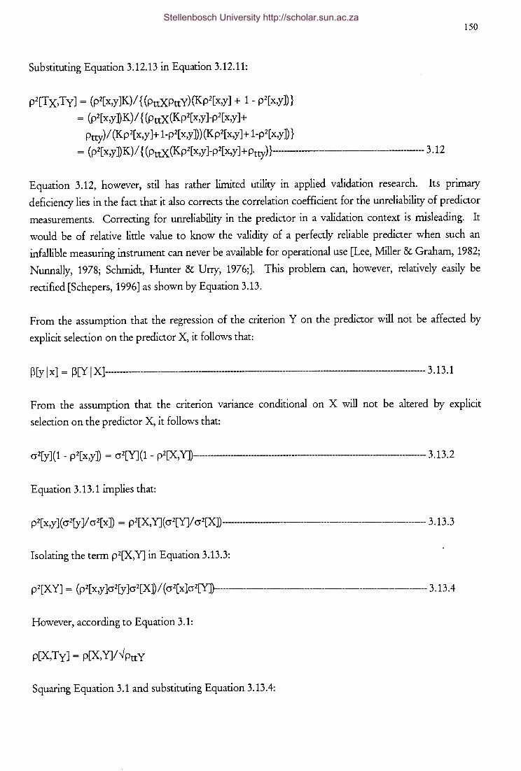
Substituting Equation 3.12.13 in Equation 3.12.11:
p2[Tx,Ty] = (p2[x,y]K)/{(pttXPttY)(Kp2[x,y] + 1- p2[x,y])}
= (p2[x,y])K)/ { (PttX(Kp2[x,y]-p2[x,y]+
Ptty)/(Kp2[x,y ]+ 1-p2[x,y])(Kp2[x,y]+ 1-p2[x,y])}
= (p2[x,y]K)/{(PttX(Kp2[x,y]-p2[x,y]+Ptty)}-------------------------------------3.12
150
Equation 3.12, however, stil has rather limited utility in applied validation research. Its primary
deficiency lies in the fact that it also corrects the correlation coefficient for the unreliability of predictor
measurements. Correcting for unreliability in the predictor in a validation context is misleading. It
would be of relative little value to know the validity of a perfectly reliable predicter when such an
infallible measuring instrument can never be available for operational use [Lee, Miller & Graham, 1982;
Nunnally, 1978; Schmidt, Hunter & Uny, 1976;]. This problem can, however, relatively easily be
rectified [Schepers, 1996] as shown by Equation 3.13.
From the assumption that the regression of the criterion Y on the predictor will not be affected by
explicit selection on the predictor X, it follows that:
p[y I X] = p[Y I X]---------------------------------------------------------------------------------------------- 3.13 .1
From the assumption that the criterion variance conditional on X will not be altered by explicit
selection on the predictor X, it follows that:
cr2[y] ( 1 - p2[ x,y ]) = cr2[Y] ( 1 - p2[X, Y])----------------------------------------------------------------------------- 3 .13. 2
Equation 3.13.1 implies that:
p2[ x,y ]( cr2[y ]/ cr2[ x ]) = p2(X,Y]( cr2[YJ/ cr2[X]) ----------------------------------------------------------------- 3.13 .3
Isolating the term p2[X,Y] in Equation 3.13.3:
p2[XY] = (p2( x,y ]cr2[y ]cr2[X]) I ( cr2( x ]cr2[Y])------------------------------------------------------------------------ 3.13. 4
However, according to Equation 3.1:
p[X,Ty] = p[X,YJI'-'PttY
Squaring Equation 3.1 and substituting Equation 3.13.4:
Stellenbosch University http://scholar.sun.ac.za
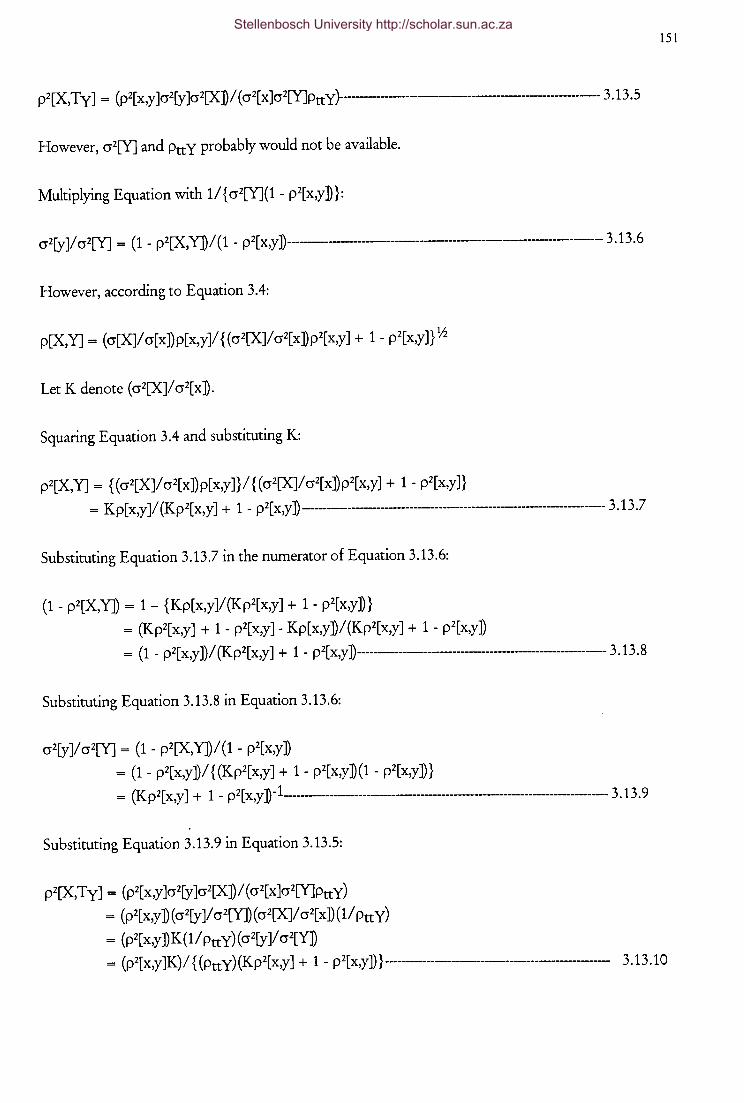
p2[X,Ty] = (p2[ x,y ]cr2[y ]cr2[X]I ( cr2[ x ]cr2[Y]ptt y}------------------------------------------- 3.13 .5
However, cr2[Y] and PttY probably would not be available.
Multiplying Equation with 11{cr2[Y](1- p2[x,y]}:
cr2[y]lcr2[YJ = (1- p2[X,Y]I(1- p2[x,y])-------------------------------------------------------- 3.13.6
However, according to Equation 3.4:
p[X,Y] = (cr[X]Icr[x])p[x,y]l{(cr2[X]Icr2[x])p2[x,y] + 1- p2[x,y]}lh
Let K denote (cr2[X]Icr2[x]).
Squaring Equation 3.4 and substituting K:
p2[X,Y] = {(cr2[X]Icr2[x])p[x,y]}l{(cr2[X]Icr2[x])p2[x,y] + 1- p2[x,y]}
= Kp[ x,y ]I (Kp2[ x,y] + 1 - p2[ x,y ]) ----------------------------------------------------------------------- 3.13 .7
Substituting Equation 3.13.7 in the numerator of Equation 3.13.6:
(1- p2[X,Y]) = 1- {Kp[x,y]I(Kp2[x,y] + 1- p2[x,y])}
= (Kp2[x,y] + 1- p2[x,y]- Kp[x,y])I(Kp2[x,y] + 1 - p2[x,y])
= ( 1 - p2[ x,y ]) I (Kp2[ x,y] + 1 - p2[ x,y ])----------------------------------------------------------- 3.13. 8
Substituting Equation 3.13.8 in Equation 3.13.6:
cr2[y]lcr2[Y] = (1- p2[X,Y])I(1- p2[x,y])
= (1- p2[x,y])I{(Kp2[x,y] + 1- p2[x,y])(1- p2[x,y])}
= (K p2[ x,y] + 1 - p 2 [ x, y ]) -1-------------------------------------------------------------------------- 3 .13 . 9
Substituting Equation 3.13.9 in Equation 3.13.5:
p2[X,Ty] = (p2[x,y]cr2[y]cr2[X]I(cr2[x]cr2[Y]ptty)
= (p2[x,y] ( cr2[y ]I cr2[Y]) ( cr2[X]I cr2[ x ]) ( 1 I Ptt y)
= (p2[x,y]K(11PnY)(cr2[y]lcr2[Y])
151
= (p2[x,y ]K)I { (PnY)(Kp2[x,y] + 1 - P2[x,y]) }--------------------------------------------------- 3.13.10
Stellenbosch University http://scholar.sun.ac.za
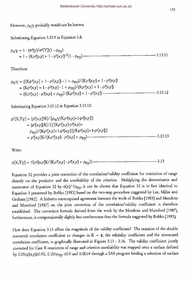
However, Ptt y probably would not be known.
Substituting Equation 3.13.9 in Equation 3.8:
PttY = 1- (cr2[y]/cr2[Y])(1- Ptty) = 1- (Kp2[x,y] + 1- p2[x,y])-1(1- Pny)-------------------------------------------------------3.13.11
Therefore:
PttY = {(Kp2[x,y] + 1- p2[x,y])- 1 + Pny}/(Kp2[x,y] + 1- p2[x,y])
= (Kp2[x,y] + 1- p2[x,y]- 1 + Pny)/(Kp2[x,y] + 1- p2[x,y])
= (Kp2[x,y]- p2[x,y] + Pny)/(Kp2[x,y] + 1- p2[x,y])------------------------------------------------- 3.13.12
Substituting Equation 3.13.12 in Equation 3.13.10:
p2[X,Ty] = (p2[x,y])K)/ {PnY(Kp2[x,y]+ 1-p2[x,y])}
= (p2[x,y])K)/ { { (Kp2[x,y]-p2[x,y]+
Pny)/ (Kp2[x,y ]+ 1-p2[ x,y ]) } (Kp2[ x,y ]+ 1-p2[x,y ]) }
= p2[ x,y ]K/ (Kp2[ x,y] - p2[ x,y] + Ptty )----------------------------------------------------------- 3 .13 .13
Write:
p[X,Ty] = --J { p2[x,y ]K/ (Kp2[x,y] - p2[ x,y] + Ptty)} --------------------------------------------------------- 3.13
152
Equation 32 provides a joint correction of the correlation/validity coefficient for restriction of range
directly on the predictor and the unreliability of the criterion. Multiplying the denominator and
numerator of Equation 32 by cr[x]/--Jptty, it can be shown that Equation 32 is in fact identical to
Equation 5 presented by Bobko [1983] based on the two-step procedure suggested by Lee, Miller and
Graham [1982]. A hitherto unrecognised agreement between the work of Bobko [1983] and Mendoza
and Mumford [1987] on the joint correction of the correlation/validity coefficient is therefore
established. The correction formula derived from the work by the Mendoza and Mumford [1987],
furthermore, is computationally slightly less cumbersome than the formula suggested by Bobko [1983].
How does Equation 3.13 affect the magnitude of the validity coefficient? The reaction of the double
corrected correlation coefficient to changes in K = ~' the reliability coefficient and the attenuated
correlation coefficient, is graphically illustrated in Figures 3.13 - 3 .16. The validity coefficient jointly
corrected for Case B restriction of range and criterion unreliability was mapped onto a surface defined
by 0.05~p[x,y]~0.90, 0.10~Ptty ~0.9 and 1~K~4 through a SAS program feeding a selection of surface
Stellenbosch University http://scholar.sun.ac.za

153
coordinates into Equation 3.13. Figures 3.13- 3.16 indicate that the amount of benefit derived from
Equation 3.13 increases as K increases and Ptty decreases. The uncorrected validity coefficient p[ x, y]
[i.e. the observed validity coefficient for the attenuating effect of both restriction of range and criterion
unreliability] provides a too conservative description of the actual correlation existing between X and
Ty. The extent to which p[x,y]underestimate p[X,Ty] increases as the restriction of range becomes
more severe and the reliability of the criterion scores declines. The corrected validity coefficient
p[X,Ty] seems to be a positive curvilinear function of p[x,y], with the degree of curvilinearity
diminishing as the attenuated validity coefficient increases. The corrected validity coefficient, similarly,
increases curvilinearly with an increase in the attenuated validity coefficient, with the degree of
curvilinearity increasing as K = cr2[X]/cr2[x] increases. Relatively more, therefore, is gained by
correcting an attenuated validity coefficient observed in the lower region of the validity scale than in the
upper region of the scale.
The findings reported here clearly indicates the dramatic consequence of correcting the observed
validity coefficient for the attenuating effect of both restriction of range and criterion unreliability,
especially when severe range restriction occurred and the criterion measures suffer from low reliability.
Not to correct the observed validity coefficient will severely underestimate the actual validity of the
selection procedure for the applicant population. Lee, Miller and Graham [1982], and Bobko [1983]
concur that all the available evidence argue in favor of jointly correcting the validity coefficient for the
attenuating effect of both range restriction and the unreliability of the criterion. Lee, Miller and
Graham [1982] found most corrected validity coefficients to be slight overestimates of the true validity
coefficient. In direct contrast to the findings reported by Lee, Miller and Graham [1982], Bobko [1983]
concludes that, on average, the double corrected validity coefficient will still underestimate the
operational validity coefficient. The research reported here does not permit any comment on bias in
the corrected validity coefficient.
A further, less serious, limitation of both Equations 3.13 and 3.12 concerns the premise that selection
can only occur directly on the predictor. Case C conditions [indirect restriction of range on the
predictor and the criterion through direct selection on a third variable] probably constitute the
predominant environment in which restriction of range corrections are required. Again, however, this
problem can relatively easily be rectified by substituting the Case B restriction of range correction
formula in the derivation of Equation 3.13 and Equation 3.12 with the appropriate Case C correction
formula [Gulliksen, 1950; Thorndike, 1949;].
Ptty
Stellenbosch University http://scholar.sun.ac.za
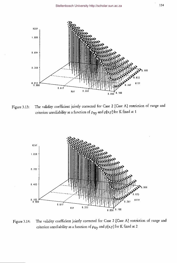
154
.900
Figure 3.13: The validity coefficient jointly corrected for Case 2 [Case A] restriction of range and
criterion unreliability as a function of Ptty and p[x,y] forK fixed at 1
RCXY
1 . DO 0
0. 7 02
0. 4 0 3 .900
0.050 0.100
Figure 3.14: The validity coefficient jointly corrected for Case 2 [Case A] restriction of range and
criterion unreliability as a function of Ptty and p[x,y] for K fixed at 2
Stellenbosch University http://scholar.sun.ac.za
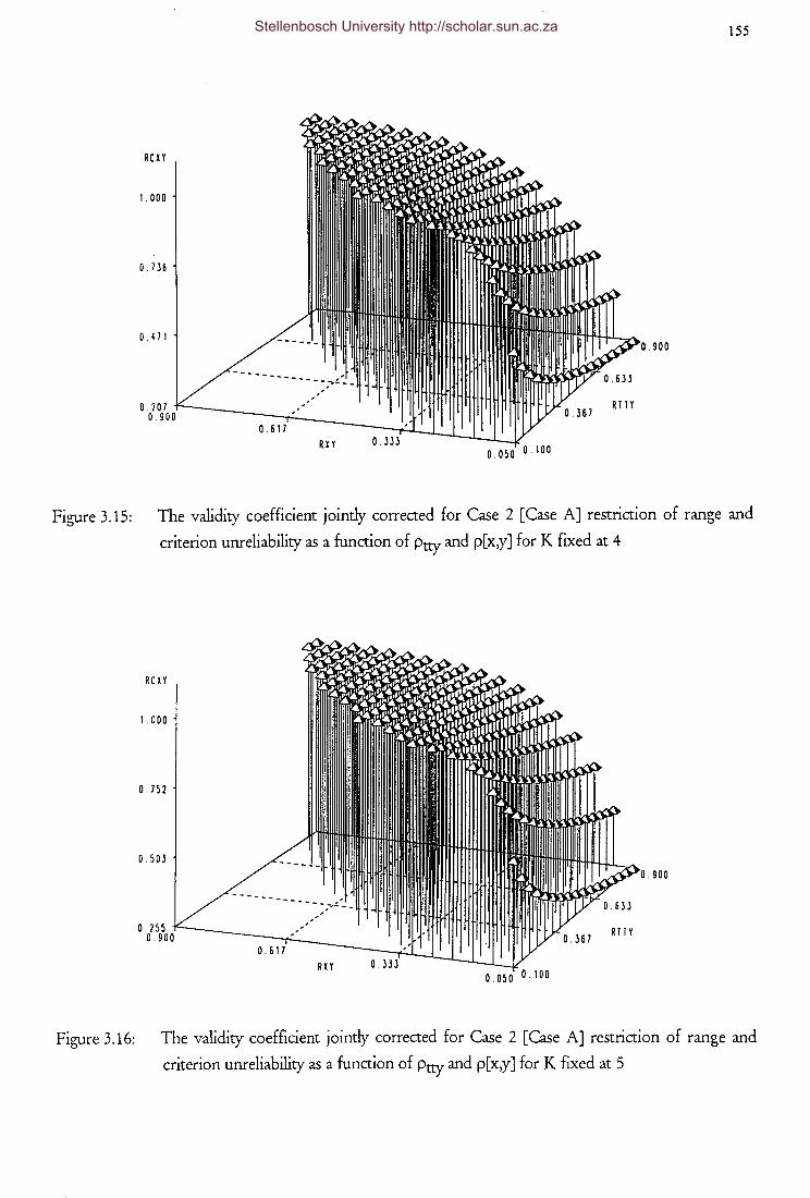
155
RCXY
1 . 000
0. 7 J6
0.01 .900
RTT Y
RXY 0.050 0.100
Figure 3.15: The validity coefficient jointly corrected for Case 2 [Case A] restriction of range and
criterion unreliability as a function of Ptty and p[x,y] forK fixed at 4
RCXY
1000
0 7 52
O.SOJ .900
0.050 0.100
Figure 3.16: The validity coefficient jointly corrected for Case 2 [Case A] restriction of range and
criterion unreliability as a function of Ptty and p[x,y] for K fixed at 5
Stellenbosch University http://scholar.sun.ac.za

156
3.5 SUMMARY
The need for correcting the validity coefficient in selection validation research for the attenuating effect
of the unreliability of the criterion measurements and/ or restriction of range was discussed.
Subsequently the derivations of correction formula for the full and partial disattenuation of the· validity
coefficient were presented. The behaviour of the partially disattenuated validity coefficient to changes
in the attenuated validity coefficient and the criterion reliability coefficient were examined graphically.
Three different conditions under which restriction of range could bias the validity coefficient were
discussed. The derivations of appropriate correction formula for the three conditions were presented.
The effect of these correction equations on the validity coefficient was examined graphically. The
robustness of the correction formula for the violation of the linearity, normality and homoscedasticity
assumptions was discussed.
The derivation of an appropriate correction formula to jointly correct the validity coefficient for Case 1
restriction of range and criterion unreliability was presented. The effect of the joint correction on the
validity coefficient was examined graphically.
~----------------------------------------------------------------·~
Stellenbosch University http://scholar.sun.ac.za

CHAPTER4
STATISTICAL INFERENCE REGARDING CORRELATIONS CORRECTED FOR THE
SEPARATE AND COMBINED ATTENUATING EFFECT OF RESTRICTION OF
RANGE AND CRITERION UNRELIABILITY
The purpose of the following chapter is firstly to provide a brief description of the place and role of
statistical inference in validation research. The function of sampling distributions of statistics in
statistical inference will subsequently be sketched. The different procedures available to establish the
necessary knowledge on the statistical properties of sampling distributions of statistics will thereafter be
discussed. A survey of the existing literature on the characteristics of the sampling distributions of
correlations corrected for the attenuating effect of predictor and criterion unreliability, criterion
unreliability, Case 1 [Case B], Case 2 [Case A] and Case 3 [Case C] restriction of range and the
combined effect of criterion unreliability and Case 2 [Case A] restriction of range will be presented.
The behaviour of the standard error of the corrected correlation coefficient, in isolation and in relation
to the standard error of the uncorrected coefficient, will finally be examined by adjusting the levels of
relevant parameters and portraying the reaction visually in three dimensional graphic representations.
4.1 INFERENTIAL STATISTICS INVALIDATION RESEARCH
Due to practical considerations, the investigation of research questions are normally conducted on
samples drawn/ obtained from larger populations. Although forced by practical considerations to
investigate only a sub-section of the population, the focus of interest, however, still is on the
[unknown] value of one or more specific parameters [8i] characterising the population and not the
values of the corresponding statistics [8 A i] characterising the sample. The statistics [8 A i] are normally
considered relevant only because they reflect, albeit with less than perfect accuracy, the parameter of
interest [assuming the sample to be representative of the population of interest]. The inability of
sample statistics/ estimators to precisely mirror the corresponding parameter in the parent population
lies in the inherent incapability of a sample to represent/ substitute its source population perfectly. The
researcher thus has to generalise beyond the obtained sample results under conditions of uncertainty.
Three basic inferential options are available:
~ obtain a point estimate [8 A] of the unknown population parameter [8]; and/ or
~ obtain a confidence interval estimate of the unknown population parameter
[810~8~8up]; and/ or
~ decide on the tenability of a hypothesis [8 = 8o] on the value of the unknown
population parameter by estimating the probability of the sample statistic
Stellenbosch University http://scholar.sun.ac.za

158
conditional on the hypothesised value of the unknown population parameter
[P[8A=8A 11e=8o]J.
Assessment of the accuracy of point estimates would be possible only if the sampling distribution of
the estimator is known or could be simulated. Similarly, the latter two options would be viable only if
the "behavior" of the sample estimator were known [i.e. could be statistically and mathematically
described] or could be simulated. Thus, either the distributional form of the sampling distribution of
the estimator must be known or an array of possible values for the sample estimator must be generated
through a series of independent samples. The distributional form of the sampling distribution of the
estimator is considered known if a mathematical model/ probability density function can be specified
that describes the sampling distribution of the estimator exactly or by approximation.
All correction formula introduced in chapter 3 [and all other statistical expressions in the preceding
chapters] were presented as population parameter and thus are, in terms of the preceding argument,
normally not directly calculable. It is, however, possible to estimate the parameter of interest by
substituting the parameters contained in the formula with the appropriate sample estimators. This
strategy rests on the critical assumption that the statistics obtained in an applied research situation may
be considered valid estimates of the respective parameters in either the unrestricted [i.e. entire] or
selected applicant populations. This in turn rests on the equally critical presumption that the
unrestricted and restricted samples of actual observations may be considered representative of the two
respective applicant populations. This in effect means that the actual applicant groups studied must be
equivalent to random samples drawn from the theoretical populations of interest. Too often, however,
there is sufficient reason to believe that this is in fact not the case [Mendoza & Mumford, 1987].
Even if these assumption would be warranted, the corrected sample correlation coefficient [p A cJ would,
however, still only reflect with less than perfect accuracy, the parameter of interest [pcJ due to sampling
error. Consequently a need for some indication on the accuracy of p A c as a point estimate of the
unattenuated parameter Pc arises. The construction of a confidence interval estimate of the unknown
corrected population parameter [Pu~Pc~Pl] would, furthermore, provide additional formal
acknowledgement of the inherent uncertainty in generalising the corrected sample correlation
coefficient beyond the confines of the validation sample. Furthermore, due to the inherent incapability
of any validation sample to represent/ substitute its source applicant population perfectly, the possibility
always exists that the corrected sample correlation coefficient is attributable purely to chance [i.e. the
possibility always exists that Pc = 0 even though p A c * 0]. The unassailableness of a defense of a
selection procedure, based on validity evidence derived from a validation sample, thus clearly depends
[amongst other things] on the magnitude of the probability of the sample statistic [pA cJ conditional on·
the hypothesised position that the unknown population parameter equals zero [i.e. P[p A c = p A c1 I p = 0].
Should the conditional probability not be sufficiently small [i.e. smaller than at least 0,05], the credibility
Stellenbosch University http://scholar.sun.ac.za

159
of the evidence lead in defense of the selection procedure will necessarily suffer. Consequently the
need also exists to estimate ab = P[p "c = p "c1 I Pc = 0].
The feasibility of actually implementing any one or more of the aforementioned three options would,
however, depend on the familiarity with the sampling distribution of the corrected correlation
coefficient.
4.2. THE NEED FOR INFORMATION ON THE SAMPLING DISTRIBUTION OF
THE VALIDITY COEFFICIENT CORRECTED FOR THE ATTENUATING
EFFECT OF THE UNRELIABILITY OF MEASUREMENTS AND/OR
RESTRICTION OF RANGE
The sampling distribution of the Pearson product moment correlation coefficient under different
sampling conditions has been well documented [Guilford & Fruchter, 1978; Hays, 1971]. The
construction of confidence intervals around point estimates and the testing of hypotheses regarding
population parameters consequently are relatively easy to perform. The traditional sampling theory,
however, is not appropriate for testing hypotheses on the corrected validity coefficient, constructing
confidence intervals around the corrected estimate or assessing the accuracy of point estimates of the
corrected parameter [Forsyth, 1971; Mendoza, Hart & Powell, 1991]. Not knowing the sampling
distribution applicable to such corrected estimates would seriously impede the ability of the validation
researcher to build a convincing argument in defense of a selection procedure. There would be simply
no way of rationally deciding whether the obtained sample results are attributable to chance or not
[Cook, Campbell & Peracchio, 1991].
Logically the same problem experienced with testing hypothesis with regards to the corrected validity
coefficient could potentially also apply to any other statistic of relevance to the argument lead in
defense of a selection procedure [e.g. the regression coefficients defining the selection decision
function], should such statistics also be affected by restriction of range and/ or criterion unreliability or
should the sampling variance of such statistics be unknown [e.g. the success ratio, SvJ.
The Standards for Educational and Psychological Testing [American Psychological Association,
American Educational Research Association & National Council on Measurement in Education, 1974,
p. 41] put forward the position that hypothesis on the statistical significance of corrected validity
coefficients should not be tested:
Stellenbosch University http://scholar.sun.ac.za

Where correlation coefficients are corrected for attenuation or restriction of range, full information relevant
to the correction should be presented. If such corrections are made, significance tests should be made with
the uncorrected correlation coefficients.
160
If the implicit argument is that the sampling distribution of the corrected correlation coefficient differs
from that of the uncorrected coefficient at least in terms of dispersion and thus that the normal test
statistic do not apply to significance tests, the statement is accurate. The statement is, however,
misleading in as far as it is implied that corrected correlation coefficients should and/ or could under no
circumstances be subjected to significance tests.
Moran [1970] indicates that hypotheses on functions of the Pearson correlation coefficient of the form
Ho: f(p[X,Y] = 0 may be tested by expressing the obtained sample estimate in terms of standard error
of the function of the correlation. Moran [1970] contends that f(pA[X,Y])/~Var(f(r[X,Y])) has,
asymptotically, a standard normal [0,1] distribution. It thus follows that significance tests on corrected
correlation/validity coefficients are possible if, but only if, an appropriate expression [or value] for the
standard error of the corrected coefficient can be derived. Similarly, the construction of standard
normal confidence intervals for corrected correlation coefficients should be a viable enterprise,
provided appropriate standard error expressions [or values] are available [Bobko & Rieck, 1980].
4.3 DIFFERENT PROCEDURES FOR INVESTIGATING THE SAMPLING
DISTRIBUTIONS OF STATISTICAL ESTIMATORS
Two fundamental approaches exist in terms of which the sampling distribution of an estimator can be
investigated. The one approach requires no assumptions about the form of the underlying population
distribution and hence is referred to as a distribution free approach. The second approach, in contrast,
starts by explicitly specifying the [actual or assumed] population distribution of the dependent variable
and consequently is known as a non-distribution free approach. The terms non-parametric and
parametric approaches are sometimes wrongfully used to refer to the aforementioned two approaches.
In the case of the correlation coefficient both approaches are, by definition, parametric in nature.
4.4 NON-DISTRIBUTION FREE ESTIMATES OF STATISTICAL ERROR
Two non-distribution free alternatives exist in terms of which the sampling distribution of an estimator
could be examined:
Stellenbosch University http://scholar.sun.ac.za

~ an experimental/ empirical method; or
~ an analytical/ mathematical method.
161
The first method uses Monte Carlo resampling from a population with a known distribution to observe
the behaviour of the sample estimator and to infer the statistical characteristics of the sampling
distribution. The second method, in contrast, derives expressions for the statistical characteristics of
the sampling behaviour of a sample estimator through mathematical analysis from explicit population
distribution assumptions.
Although both methods seem suited to examine the sampling distribution of the corrected correlation
coefficient under specific known parametric conditions, the analytical method seems to dominate more
recent non-distribution free investigations. Kelley [1947] distinguishes the following analytic methods
in terms of which the standard error of a statistic can be derived, if the statistic is a function of a
statistic with a known standard error:
~ the binomial expansion method;
~ substitution of statistical deviations for calculus differentials method;
~ expanding by a Taylor series method or Delta method; and
~ logarithmic differentials method.
The Delta method [Rao, 1973] seems to be the preferred analytical approach.
4.4.1 Delta Method
Assume an estimator which is a function of the Pearson product-moment correlation p"[X,Y]. Let
such an estimator be denoted by f(p"[X,Y]). Using the Taylor expansion Kendall and Stuart (1977, p.
247] derive the expression shown as Equation 4.1 for the variance of f(p "[X,Y]).
cr2 { f(p "[X,Y])} = .L[f'i(P)]2Var[ri]+Lf'i(p)f'j(p)Cov[ri,rj] +[terms of order n-2 or less]---------- 4.1
Expressions for the asymptotic variance of p" [X,Y] and the asymptotic covariance between two
correlations computed on the same sample are required to execute Equation 4.1 [Bobko & Rieck,
1980]. The asymptotic variance of the correlation coefficient obtained from a bivariate normal
population with parameter p[X,Y], is given by Equation 4.2 [Kendall & Stuart, 1977, p. 251].
cr2 (p "[X,Y]) = ( 1-p2[X, YJ)2 In-------------------------------------------------------------------------------------- 4.2
Stellenbosch University http://scholar.sun.ac.za

162
Assuming multivariate normality, the asymptotic covariance between two correlations computed on the
same sample is shown as Equation 4.3 [Kelley, 1947, p. 553] for the case where one variable is common
to both correlations.
cr[ r[X,Y],r[X,Z]]=
{ p[X,Y](1-p2[Y,Z]-p2[X,Z])-'h (p[Y,Z]p[X,Z]) (1-p2[Y ,Z]-p2[X,Y]-p2[X,Z])} In------4.3
4.5 DISTRIBUTION FREE ESTIMATES OF STATISTICAL ERROR
The trouble is that analytically or empirically derived standard errors for estimators more complex than
the traditional descriptive statistics often do not exist. No mathematical expression thus exists that
captures the capricious behaviour of the statistical estimator across repeated samples from the same
parent population. Furthermore, the parametric assumptions underlying the analytically derived
standard error expressions are often not satisfied, thus raising suspicion on the applicability of the
expressions. Distribution free resampling techniques represent a feasible solution to these problems.
A Monte Carlo approach would, however, normally not present a feasible solution in an applied
context since information on the population distribution and its parameters are normally not available
in applied validation research.
The bootstrap and jackknife are the two most popular data-resampling techniques used in inferential
statistical analysis [Shao & Tu, 1995].
4.5.1 Bootstrap Estimates Of Statistical Error
The bootstrap represents an approach to the investigation of the sampling behavior of sample
estimators which:
>- relieves the analyst from having to make any parametric assumptions about the
form of the underlying population distribution; and
>- enables the analyst to proceed with inferential analysis even if no mathematical
expressions on the sampling behaviour of the estimator exist.
The term bootstrap is derived from the expression to pull yourself up by your own bootstraps generally
believed to originate from one of Rudolph Raspe's Adventures of Baron von Miinchhausen [Efron &
Tibshirani, 1993]. The term appears to be appropriate since the bootstrap procedure in essence
Stellenbosch University http://scholar.sun.ac.za

163
represents a seemingly impossible attempt to simulate the behaviour of a sample statistic across a large
number of independent samples taken from a single parent population from data available only in a
single sample [Diaconis & Efron, 1983; Efron, 1982; Efron & Tibshirani, 1993; Lunneborg, 1985; Shao
&Tu, 1995].
Assume a population I1 of potential observations characterised by the parameter 9. Assume further a
random sample T of n observations drawn independently from population TI. Should the statistic 9"
corresponding to the parameter 9 in I1 be calculated, an estimate of 9 would be obtained. A succession
of m [bootstrap] samples Tbi of size n are subsequently drawn randomly with replacement from the
original sample T. From each bootstrap sample Tbi· a bootstrap estimate 9" bi is obtained. The
fundamental bootstrap proposition is that the distribution of the bootstrap estimates 9"bi [i.e. the
sampling distribution of 9 "b] will provide a sufficient approximation of the [true] sampling distribution
derived analytically/theoretically from specific parametric assumptions and/ or derived empirically
through the classical Monte Carlo generation of m independent random samples Ti of size n from I1
[Diaconis & Efron, 1983; Efron, 1982; Efron & Tibshirani, 1993; Lunneborg, 1985; Shao & Tu, 1995].
From this conjecture follows that as the number of bootstrap samples approach infinity, the standard
deviation of the distribution of bootstrap estimates, shown as Equation 4.4, approaches the standard
error of the estimator e".
cr[9 "] ~ cr[9 "b] = p:::(e "bi-(L9 "b/ m))21 m-1} lh ------------------------------------------------------------ 4.4
4.5.1.1 Bootstrap Confidence Intervals
Once the standard error of the estimator is obtained from the distribution of the bootstrap estimates
e "bi [i.e. the standard deviation of the bootstrap distribution], a parametric bootstrap confidence
interval around the obtained sample estimate 9" can be computed under the assumption that the
sampling distribution of 9 "b sufficiently corresponds to a familiar mathematical model [e. g. Gauss or
Student distributions]. Assuming the sampling distribution to be approximately standard normal, a
parametric confidence interval for the unknown parameter 9 can be obtained, with coverage probability
equal to [1-a], through Equation 4.5 [Efron & Tibshirani, 1986; Efron & Tibshirani, 1993; Thompson,
1991].
9 E 9 " ± cr " [ 9 "b]Za/ 2 -------------------------------------------------------------------------------- 4 5
Stellenbosch University http://scholar.sun.ac.za

164
Efron & Tibshirani [1993] suggest that the standard parametric confidence interval can be improved
for small samples by substituting the standard normal critical values [given a] with critical values
derived from the Student t distribution at appropriate degrees of freedom.
The bootstrap-t confidence interval differs from the aforementioned approaches in as far as it does not
require apriori distributional assumptions. The bootstrap-t method requires the generation of m
bootstrap samples. For each bootstrap sample the bootstrap estimate 8~bi is standardised by deviating
it from the initial sample estimate 8 ~ and expressing the deviation in terms of the estimated standard
error of the bootstrap estimate [i.e. Z=(8~bi-8A)/cr~[8~bi]J. The estimation of the standard error of
8~bi would require a further g bootstrap samples drawn with replacement from the ith bootstrap
sample; hence a potentially formidable total number of mg bootstrap samples are required to construct
a bootstrap-t confidence interval [Shao & Tu, 1995]. The bootstrap-t confidence interval is
subsequently constructed by "reading off" the Z-values corresponding to the 100[a/2]th and 100[1-
a/2]th percentiles and inserting them with the sample estimate 8 ~ and the bootstrap estimate of the
standard error into Equation 4.6 [Efron & Tibshirani, 1993].
8 E 8 ~ ± cr A[8 ~b]Za/2 -------------------------------------------------------------------------------- 4.6
Whereas the standard normal and Student-t bootstrap confidence intervals are symmetric around the
point estimate 8 ~, the bootstrap-t confidence limits can be positioned asymmetric around 8 ~. Efron
and Tibshirani [1993], however, warn that in practice the bootstrap-t can give somewhat erratic results.
An alternative approach to the estimation of a confidence interval suggested by Efron [1982]
determines the 100[a/2]th and 100[1- a/2]th order values or percentiles directly from the rank-ordered
bootstrap estimates 8 ~ bi. An empirical confidence interval could thus be defined by identifying the
appropriate [depending on the chosen a-level] percentiles in the bootstrap sampling distribution
without making any parametric assumptions. The empirical confidence interval limits consequently
would not necessarily lay symmetrically around 8A. Efron [1982] and Efron and Tibshirani [1986;
1993] refers to this non-parametric approach as the percentile method. However, should the bootstrap
estimate 8 A bi follow a normal distribution, the percentile and standard methods would deliver
equivalent confidence intervals [Efron & Tibshirani, 1986].
A number of modifications to the percentile bootstrap confidence interval discussed above have been
suggested [Efron, 1982; Shao & Tu, 1995] to combat the reported tendency [Efron, 1982; Rasmussen,
1987; Strube, 1988] for the aforementioned non-parametric bootstrap methodology to deliver overly
restricted confidence intervals and thus overly liberal Type I error rates. Efron [1982] firstly suggests
an adjusted bootstrap interval, obtained by extending the percentile bootstrap interval by [(n+2)/(n-
1)]lh in both directions. As an alternative solution Efron [1982] suggests a bias-corrected confidence
----------------------------------------------------------------~
Stellenbosch University http://scholar.sun.ac.za

165
[BC] interval which differs in length from the percentile interval. The latter adjustment procedure
modifies the percentile interval for bias in the sample estimate 8" by shifting the confidence interval
limits depending on the location of the obtained statistic [8"] in relation to the median bootstrap
statistic [Me[8 "bi]J. The adjustment is accomplished through the quantity z" 0 representing a bias
correctiOn constant. The bias-correcting constant z" 0 equals the normalised standard score
corresponding to the percentile rank of 8" in the bootstrap distribution [i.e. the standard score which
cuts off an area in the standard normal distribution equal to the area below 8"bi in the bootstrap
distribution] [Shao & Tu, 1995]. The upper and lower [1-a]100% BC confidence interval limits
[8"b[lo] & 8"b[up]J are given by the bootstrap estimates q\i corresponding to a1100th and a2100th
percentiles in the bootstrap distribution, where a1 and a2 are given by Equation 4.7 [Efron &
Tibshirani, 1993].
a1 = <l>{z"o+za/2} l r ---------------------------------------------------------------------------------------- 4.1
a2 = <l>{z"o+z1-a/2} J
where <l> indicates the standard normal cumulative distribution function; and
Za/2 indicates the standard normal score corresponding to a percentile rank of 100[a/2]
Efron & Tibshirani [1993], in addition, suggest a bias-corrected and accelerated confidence [BCaJ
interval. The BCa interval limits are also given by percentiles of the bootstrap distribution. The upper
and lower [1-a]100% BCa confidence interval limits [8\[lo] & 8"b[up]J are given by the bootstrap
estimates q" bi corresponding to a 11 OOth and a 21 OOth percentiles in the bootstrap distribution [Shao
& Tu, 1995], where a1 and a2 are given by Equation 4.8 [Efron & Tibshirani, 1993].
a1 = <l>{z"o + (z"o+Za/2)/(1-a"[z"o+Za/2])} l r -------------------------------------- 4. 8
a2 = <l>{z"o + (z"o+z1-a/2)/(1-a"[z"o+z1-a/2])}J
where <l> indicates the standard normal cumulative distribution function; and
Za/2 indicates the standard normal score corresponding to a percentile rank of 100[a/2]
The quantities a" represents an acceleration constant whereas z" 0 still represent a bias-correction
constants. The quantity a" indicates [Efron & Tibshirani, 1993, p.186]:
Stellenbosch University http://scholar.sun.ac.za

... the rate of change of the standard error of eA ·with respect to the true parameter value e. The standard
normal approximation e A :::::N(e,se2) assumes that the standard error of e A is the same for all e. However this
is often unrealistic and the acceleration constant a A corrects for this.
166
Although the acceleration constant a is considered difficult to estimate [Shao & Tu, 1995], Efron &
Tibshirani [1993, p. 186] nonetheless offer Equation 4.9 as one possible way of obtaining an
approximation based on the jackknife [see ,4.5.2].
a A = { L ( 8 j -8 jJ 3} I { 6[L ( 8 j-8 jJ "]3 I 2} ----------------------------------------------------------------------- 4. 9
where 8 A ji represent jackknife estimates of 8; and
If a A and z A 0 equal zero the BCa interval becomes the percentile interval since a 1 and a 2 would then
equal <l>{zal2} and <l>{z1-al2} respectively which equals al2 and 1-al2 [Efron & Tibshirani, 1993].
The effect of all the modifications suggested to the standard percentile procedure, is to reduce the
inflation of the Type I error rate above the chosen error rate [a].
4.5.1.2 Bootstrap Hypothesis Testing
Investigating the statistical significance of the observed correlation coefficient through the testing of
the null hypothesis HQ: p = 0 probably constitutes the more prevalent form of hypothesis testing in
validation research. Conventional hypothesis testing procedures provide an adequate statistical tool to
decide on the validity of Ho. Bootstrap approaches to hypothesis testing are consequently not essential
in the conventional case. By contrast, however, investigations on the statistical significance of
corrected correlation coefficients through the testing of Ho: Pc = 0 might benefit from the availability
of hypothesis testing procedures with the bootstrap. A non-distribution free bootstrap hypothesis test
could be conducted by calculating the standard deviation of the distribution of bootstrap estimates,
converting the observed rc to a standard score and, assuming the test statistic to follow the standard
normal distribution [Moran, 1970], determine the conditional probability of the sample result under the
assumption of Ho. A one-sample distribution free bootstrap method to investigate the preceding null
hypothesis would require the following steps:
~ choose a null distribution for the sample data under Ho;
~ calculate the appropriate test statistic on the observed corrected correlation;
Stellenbosch University http://scholar.sun.ac.za

167
>- generate n bootstrap samples;
>- evaluate the test statistic on each bootstrap sample; and
>- estimate the observed exceedence probability [ ab] or achieved significance level
[ASL] and compare to the critical exceedence probability [acJ.
Simulating a null distribution for the sample data under Ho, however, seems to present a practical
problem.
Alternatively, a hypothesis test on the significance of a corrected correlation could be performed by
constructing a bootstrap confidence interval and by inspecting the interval to see whether it contains
zero or not. Should the latter outcome occur, the null hypothesis would be rejected, whereas the first
outcome would result in the conclusion that the observed corrected correlation is not significant at the
chosen significance level [Efron & Tibshirani, 1993].
4.5.1.3 Bootstrap Sample Size Requirements
The bootstrap is a computer intensive procedure. It in essence substitutes elegant and sophisticated
analytical/theoretical argument with brute computational power [Efron, 1982; Thompson 1991].
Efron [1982; 1987; 1988] suggests that as few as ten or twenty, but seldom more than two hundred,
bootstrap replications are needed to give an acceptable bootstrap estimate of the standard deviation of
the bootstrapped eAb distribution [i.e. the standard error of eAb as an approximation of cr[8A]].
Bootstrap confidence intervals, in contrast, require a substantial increase in the number of iterations.
In excess of 2000, but seldom less than 1000, iterations are required.
In the case of the corrected correlation coefficient, more than one bootstrap sample per iteration could
be required. The precise number of bootstrap samples required per iteration would depend on the
measurement design on which the computational version of the correction formula is based.
Furthermore, as was indicated earlier, if nested bootstrap sampling is required [to estimate crA[8Abi]J
the number of samples drawn will increase dramatically.
4.5.2 Jackknife Estimates Of Statistical Error
Quenouille [in Efron & Gong, 1983] is generally credited with originating the jackknife as a non
parametric device for estimating bias. This initial groundwork was subsequently further developed in
Stellenbosch University http://scholar.sun.ac.za

168
the 1950's by John W T ukey of Princeton University and the Bell Laboratories. The term jackknife was
conceived by Tukey [1956] to convey the idea that the method is an all-purpose statistical tool
applicable to a wide variety of estimators [Diaconis & Efron, 1983]. Like the bootstrap, the historically
older jackknife generates a sampling distribution for the statistic/ estimator of interest [8 A] by
resampling the original sample of size n [Thompson, 1991]. The jackknife accomplishes this by
removing one observation at a time from the original sample and then recalculating the
statistic/estimator [8Aj; i=1, 2, ... , n] for each of the resulting subsamples of size [n-1] [Diaconis &
Efron, 1983; Efron & Gong, 1983; Shao & Tu, 1995]. The variability of the statistic/estimator across
all [n-1] subsamples can then be assessed. The central postulate underlying the jackknife is that the
variability of 8 A j across the jackknife samples will approximate the variability in 8 A that would be
obtained should t [t~oo] independent random samples of size n be selected from the population [i.e.
cr2[8Aj] = cr2[8A]]. The jackknife estimate of the standard error of SA is defined by Equation 4.10
[Efron & Tabshirani, 1993; Shao & Tu, 1995].
cr[8 A] = cr[8 A b] = { (n-1/ n)L(8 A ji-(L8 Aj/ n))2} lh -------------------------------------------------------------- 4.10
The jackknife has the advantage over the bootstrap that it requires less calculations than the bootstrap.
Generally, however, the bootstrap is considered superior to the jackknife for the estimation of standard
errors and confidence intervals [Diaconis & Efron, 1983; Efron, 1982; Thompson, 1991].
4.6 EXPRESSIONS FOR THE STANDARD ERROR OF THE PEARSON
CORRELATION COEFFICIENT
4.6.1 Obtained, Uncorrected First-Order Pearson Correlation Coefficient
The sampling distribution of the Pearson product moment correlation coefficient is dependant on the
size of the sample, the population distribution and the value of the population parameter p [Guilford &
Fruchter, 1978; Hays, 1973]. When the hypothesis Ho: p[X,Y] = 0 is true, and the population can be
assumed to be bivariate normal in its distributional form, the sampling distribution of p A [X, Y]
approaches a normal [0;1/v'(n-1)] distribution as sample size increases. However, if sampling from a
bivariate normal population with p[X,Y] = 0, the t ratio shown as Equation 4.11 will be distributed as
Student's t distribution with n-2 degrees of freedom [Guilford & Fruchter, 1978; Hays, 1971].
t = (p A [X,Y]v'n-2) I v' ( 1-p A 2[X,Y]) -------------------------------------------------------------------------------- 4.11
Stellenbosch University http://scholar.sun.ac.za

169
If, however, the population correlation p[X,Y] :t:. 0 the sampling distribution of pA[X,Y] tends to be
skewed, with this tendency intensifying the more rho departs from zero. For virtually any value of rho
in a bivariate normal population, though, Fisher transformations of pA[X,Y]to ZpA [shown as Equation
4.12] will be distributed approximately normal with mean 0,5ln{(1+pA[X,Y])/(1-pA[X,Y])} and variance
[approximately] 1/(n-3) [Hays, 1971] or, as a slightly less rough approximation, {1/(n-1)}+{(4-
p A2)/(2(n-1)2)} [Stuart & Kendall, 1977].
Zp A = O,Sln { ( 1 + p A [X,Y])/ ( 1-p A [X,Y])} ------------------------------------------------- 4.12
The fit of the Gaussian curve improves as the absolute value of p[X,Y] decreases and the sample size
increases [Guilford & Fruchter, 1978; Hays, 1971].
Asymptotically [i.e. when the size of samples drawn from I1 approach infinity] the variance of the
correlation under conditions of a bivariate normal population is shown as Equation 4.13 [Bobko &
Rieck, 1980; Kendall & Stuart, 1977].
cr2[p A [X, Y]] = ( ( 1-p[X, Y])2)2n -1-----------------------------------------------------------------------------------4.13
Stuart and Kendall [1977, p. 251], however, warn:
The use of the standard error to test a hypothetical non-zero value of p is not, however, to be recommended,
since the sampling distribution of r tends to normality very slowly.
When examining the effect of statistical corrections for restnctwn of range and/ or random
measurement error applied to the correlation coefficient, the question naturally arises how the sampling
behaviour of the correlation is affected by the correction. As the preceding argument indicates,
variability represents an important facet of the sampling behaviour of any statistic. However, when
comparing the standard error of the attenuated correlation coefficient [i.e. the uncorrected coefficient]
to the standard error of the corrected correlation, the [rather crucial] dilemma emerges what estimate of
the standard error of the Pearson correlation coefficient should serve as the appropriate benchmark.
The choice of the expression in terms of which the standard error of the corrected correlation is
estimated will probably significantly affect the conclusions on the effect of the statistical corrections on
the sampling behaviour of the corrected coefficient. The square root of the asymptotic variance of the
correlation [Equation 4.13] seems to be the expression most often used for comparison purposes
within the aforementioned context [Allen & Dunbar, 1990; Bobko, 1983; Bobko & Rieck, 1980;
Forsyth & Feldt, 1969; Hakstian, Schroeder & Rogers, 1988; Hakstian, Schroeder & Rogers, 1989].
The square root of Equation 4.13 will consequently also be used in all subsequent analyses when an
estimate of the standard error of the uncorrected correlation coefficient is required. The choice of
Equation 4.13 as benchmark is, however, not without criticism [Stuart & Kendall, 1977]. The standard
Stellenbosch University http://scholar.sun.ac.za
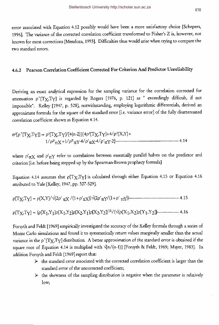
170
error associated with Equation 4.12 possibly would have been a more satisfactory choice [Schepers,
1996]. The variance of the corrected correlation coefficient transformed to Fisher's Z is, however, not
known f?r most corrections [Mendoza, 1993]. Difficulties thus would arise when trying to compare the
two standard errors.
4.6.2 Pearson Correlation Coefficient Corrected For Criterion And Predictor Unreliability
Deriving an exact analytical expression for the sampling variance for the correlation corrected for
attenuation pA[Tx,Ty] is regarded by Rogers [1976, p. 121] as " exceedingly difficult, if not
impossible". Kelley [1947, p. 528], notwithstanding, employing logarithmic differentials, derived an
approximate formula for the square of the standard error [i.e. variance error] of the fully disattenuated
correlation coefficient shown as Equation 4.14.
cr2[pA[Tx,Ty]] = p2[Tx,TyY[4(n-2)]{4p2[Tx,Ty]+4/p2[X,Y]+
1/ p2'ttX + 1/ p2'tty-4/ p 'ttX-4/ pItt y-2}-------------------------------------------------- 4.14
where p'ttX and p'ttY refer to correlations between essentially parallel halves on the predictor and
criterion [i.e. before being stepped up by the Spearman-Brown prophecy formula]
Equation 4.14 assumes that p[Tx,Ty] is calculated through either Equation 4.15 or Equation 4.16
attributed to Yule [Kelley, 1947, pp. 527-529].
p[Tx,Ty] = p[X,Y]/"(2p' ttX /(1 + p'ttX))"(2p'tty/(1 + p' ttY)}------------------------------------- 4.15
Forsyth and Feldt [1969] empirically investigated the accuracy of the Kelley formula through a series of
Monte Carlo simulations and found it to systematically return values marginally smaller than the actual
variance in the pA[Tx,Ty] distribution. A better approximation of the standard error is obtained if the
square root of Equation 4.14 is multiplied with "[n/(n-1)] [Forsyth & Feldt, 1969; Mayer, 1983]. In
addition Forsyth and Feldt [1969] report that:
};;> the standard error associated with the corrected correlation coefficient is larger than the
standard error of the uncorrected coefficient;
};;> the skewness of the sampling distribution is negative when the parameter is relatively
low;
Stellenbosch University http://scholar.sun.ac.za
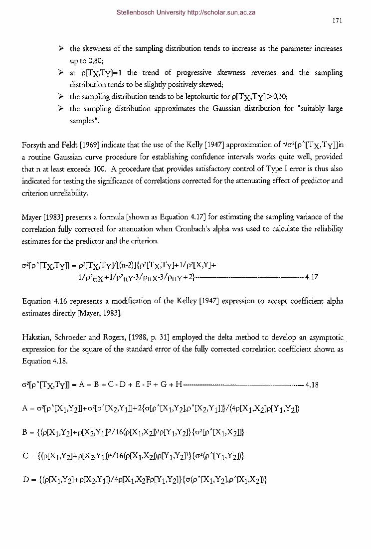
171
);> the skewness of the sampling distribution tends to increase as the parameter increases
up to 0,80;
);> at p[Tx,Ty]=1 the trend of progressive skewness reverses and the sampling
distribution tends to be slightly positively skewed;
);> the sampling distribution tends to be leptokurtic for p[Tx,Ty] >0,30;
);> the sampling distribution approximates the Gaussian distribution for "suitably large
samples".
Forsyth and Feldt [1969] indicate that the use of the Kelly [1947] approximation of .Vcr2[pA[Tx,Ty]]in
a routine Gaussian curve procedure for establishing confidence intervals works quite well, provided
that nat least exceeds 100. A procedure that provides satisfactory control of Type I error is thus also
indicated for testing the significance of correlations corrected for the attenuating effect of predictor and
criterion unreliability.
Mayer [1983] presents a formula [shown as Equation 4.17] for estimating the sampling variance of the
correlation fully corrected for attenuation when Cronbach's alpha was used to calculate the reliability
estimates for the predictor and the criterion.
cr2[pA[Tx,Ty]] = p2[Tx,TyY[(n-2)]{p2[Tx,Ty]+1lp2[X,Y]+
11 P2ttX + 11 P2tt y-3 I PttX-3 I Ptt y + 2} --------------------------------------- 4.17
Equation 4.16 represents a modification of the Kelley [1947] expression to accept coefficient alpha
estimates directly [Mayer, 1983].
Hakstian, Schroeder and Rogers, [1988, p. 31] employed the delta method to develop an asymptotic
expression for the square of the standard error of the fully corrected correlation coefficient shown as
Equation 4.18.
cr2[p A[Tx,Ty]] = A + B + c- D + E - F + G + H -------------------------------------------------------4.18
Stellenbosch University http://scholar.sun.ac.za
172
Equation 4.18 assumes that PttX and PttY represent test-retest reliability coefficients. The expression
derived by Hakstian, Schroeder and Rogers, [1988] is derived similarly to the formula [Equation 4.19]
developed by Kristof [1982]. Kristof [1982, p. 109] derives the following expression for the asymptotic
variance of pA[Tx,Ty]--ln:
cr2[pA[Tx,Ty]--Jn] = p2[Tx,Ty]{p2[Tx,Ty]+(t22/(tH-t22))2 +
(t44/ (t33-q4))2-(q 1/ (q 1-t22))-(t33/ (t33-q4))+
( ( t 11 t 3 3) It 213) } -------------------------------------------------------------------------------- 4.19
Where:
and crij represent covariance terms in a 4x4 matrix defined by two essentially parallel parts [Y 1 & Y 2J of
Y and two essentially parallel parts [X 1 & X2J of X
The expressions are not equivalent, however, due to differences in the measurement design in terms of
which the correlation coefficients corrected for predictor and criterion unreliability are estimated. The
Hakstian, Schroeder and Rogers, [1988] expression presupposes a design in which two measures X and
Y are administered at time 1 to yield X 1 and Y 1 but then re-administered after a suitable period of time
to yield X2 andY 2· In terms of this design an estimate of the fully disattenuated correlation coefficient
p[Tx,Ty] is obtained through Equation 4.20.
Stellenbosch University http://scholar.sun.ac.za
173
The Kristof [1982] formula, in contrast, assumes a measurement design in which two measures X and
Y have been applied once and subsequently divided into two essentially equivalent parts [X 1 & X2, and
Y 1 & Y 2l Kristof [1982] also examines the asymptotic variance of p A[Tx,Ty] if the less stringent
assumption is made that the test and criterion had been divided into two congeneric instead of
essentially parallel parts
4.6.3 Pearson Correlation Coefficient Corrected For Criterion Unreliability Only
Kelley [1947, p. 529], assuming the computational formula to be Equation 4.21, derived, through
logarithmic differentials, an approximate formula for the square of the standard error [i.e. variance
error] of the partially disattenuated correlation coefficient shown as Equation 4.22.
p [X, T y] = p[X, Y]/...; ( 2 pItt y I ( 1 + pItt y)) ---------------------------------------------------------------------- 4.21
cr2[p A[X,Ty ]] = p2[X,Ty]/ (n-2)(p2[X,Ty ]+p-l[X,Y]-p'-ltty+4p'-2uy-5/ 4)----------------------- 4.22
where p'ttX and p'ttY refer to correlations between essentially parallel halves on the predictor and
criterion [i.e. before being stepped up by the Spearman-Brown prophecy formula]
The reaction of Kelley's approximation of the standard error of the partially disattenuated correlation
coefficient to changes in the attenuated correlation, the reliability coefficient and sample
graphically depicted in Figure 4.1 and Figure 4.2. Figures 4.1 -4.2 reveal that the standard error:
>- decreases curvilinearly as Ptt y increases;
. . SlZe lS
>- increases as the attenuated correlation increases at low values of PttY but decreases
as the attenuated correlation increases at low values of p ttYi
>- decreases as n increases for any p[X,Y] PttY combination.
Figure 4.3 and Figure 4.4 depict the reaction of the standard error of the partially disattenuated
correlation expressed in terms of the standard error of the uncorrected coefficient [i.e. V =
cr[pA cJ/cr[p"]J to changes in p[X,Y], p ttY and n. Figures 4.3 - 4.4 suggest V to increases as the
attenuated correlation increases, but with the rate of increase decreasing as Ptt y irrreases. V also
seems to be negatively related to sample size.
Stellenbosch University http://scholar.sun.ac.za
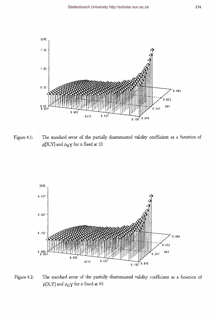
Figure 4.1:
Figure 4.2:
174
SERC
1. 52
1. 02
0.960
0. 347 RXY
0.182 0.040
The standard error of the partially disattenuated validity coefficient as a function of
p[X,Y] and PttY for n fixed at 10
SERC
0. 4 57
0.307
0 15 7 0.960
0.653
0. 008 ,-'--l.-L~~~::.Q~~~~~ffj!~~Jl~l 0. 947 0. 6 92 ,'
RIIY 0.437
0. 34 7 RXY
0.182 0.040
The standard error of the partially disattenuated validity coefficient as a function of
p[X,Y] and PttY for n fixed at 90
Stellenbosch University http://scholar.sun.ac.za

Figure 4.3:
Figure 4.4:
5. 71
4. 15
2.59
1. 0 3 0. 947
RIIY
0.347 RXY
0.182 0.040
V = cr[p ~ ,]/ cr[p ~] as a function of p[X,Y] and Pn y for n fJXed at 10
5. 16
3. 7 5
2.H
0.93 0. 947
0.653
RXY
0.182 0.040
V = cr[p ~ cJ/ cr[p ~] as a function of p[X,Y] and Pn y for n fixed at 90
175
0.960
0.960
Stellenbosch University http://scholar.sun.ac.za

176
An interesting habit of V which Figure 4.4 manages to uncover is that V drops below 1 [i.e. the
standard error of the corrected coefficient is in fact smaller than that of the attenuated correlation] in a
small region characterised by high p[X,Y] and Ptt y values. As n increases the region gradually seems to
expand to lower p[X,Y] and PttY values. Whether this habit is attributable to Equation 4.13's known
weakness in the upper region of the p[X,Y] scale, is uncertain.
Bobko & Rieck [1980, p. 388] derived, through the delta method, expressions for an approximation of
the square of the standard error of a partially disattenuated correlation coefficient shown as Equations
4.23, 4.24 and 4.25. Three different formula are presented as a function of the measurement design,
specifically the method used to calculate the criterion reliability coefficient;
>- PttY obtained from the same data set as p[X,Y] [Case I; Equation 4.23];
>- PttY obtained from an independent data set [Case II; Equation 4.24]; and
>- Ptt y accepted a priori on theoretical grounds or previously accepted knowledge
[Case III; Equation 4.25].
cr 2[ p ' [X, T y ]] = [A+ B-C] ------------------------------------------------------------------------------------------------- 4. 23
cr 2 [ p ' [X, T y ]] = [A+ B ]------------------------------------------------------------------------------------------------- 4. 2 4
cr 2[ p ' [X, T y ]] = [A]--------------------------------------------------------------------------------------------------------- 4. 25
Where:
C = (n)-1(Ptt y)-2p[X,Y]{ptt y(1-2p2[:X, Y])-(0,5p2[X, Y])(1-2p2[X,Y]-p2ttY)}
Figures 4.5 - 4.10 depict the reaction of the standard error of the partially disattenuated correlation
coefficient calculated through Equations 4.23 - 4.25 to changes in the attenuated correlation, the
reliability coefficient and sample size. When PttY is obtained from the same group as p[X,Y], Figures
4.5 - 4. 6 suggest that cr[p 'cJ: >- curvilinearly increases as the attenuated correlation increases at low values of Ptt y
but gradually reverses the trend as PttY increases until at high values of PttY' cr[p 'cJ moderately decreases as p[X,Y] increases;
>- increases as Ptt y decreases;
>- peaks at the maximum p[X,Y] value possible, given PttY;
Stellenbosch University http://scholar.sun.ac.za
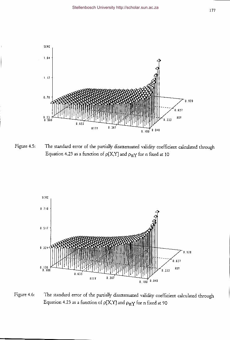
Figure 4.5:
Figure 4.6:
177
S£RC
1.64
1. 17
0. 70 0.920
-----0.627
0.333 RXY
0.100 0.040
The standard error of the partially disattenuated validity coefficient calculated through
Equation 4.23 as a function of p[X,Y] and PttY for n fixed at 10
S£RC
0 7 10
0 5 17
0. 324 0 920
0.627
0.333 RXY
RTTY 0.100 0.040
The standard error of the partially disattenuated validity coefficient calculated through
Equation 4.23 as a function of p[X,Y] and PttY for n fixed at 90
Stellenbosch University http://scholar.sun.ac.za
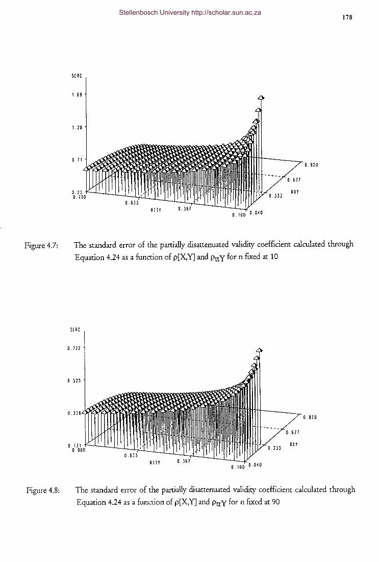
Figure 4.7:
Figure 4.8:
178
SERC
1 . 6 9
1 . 20
0. 7 1 0.920
O.JJJ RXY
0.100 0.040
The standard error of the partially disattenuated validity coefficient calculated through
Equation 4.24 as a function of p[X,Y] and PttY for n fixed at 10
SERC
0 722
0 52 5
0.920
0. 6 2 7
O.JJJ RXY
RT TY 0.100 0.040
The standard error of the partially disattenuated validity coefficient calculated through
Equation 4.24 as a function of p[X,Y] and PttY for n fixed at 90
Stellenbosch University http://scholar.sun.ac.za

Figure 4.9:
179
SERC
0.998
0.683
0.920
O.JJJ RXY
0.100 0.040
The standard error of the partially disattenuated validity coefficient calculated through
Equation 4.25 as a function of p[X,Y] and PttY for n fixed at 10
SERC
O.JJJ
0. 228
0.920
----0.627
O.JJJ RXY
0.100 0.040
Figure 4.10: The standard error of the partially disattenuated validity coefficient calculated through
Equation 4.25 as a function of p[X,Y] and PttY for n fixed at 90
Stellenbosch University http://scholar.sun.ac.za

180
~ decreases as sample size increases.
The same conclusions also seem to apply to Figures 4.7 - 4.8 portraying the behaviour of cr[p A cJ when
PttY is obtained from an independent group. In contrast, the behaviour of cr[pA cJ when PttY is
accepted a priori on theoretical grounds or previously accepted knowledge, seems to be slightly
dissimilar to that observed under the two previous measurement designs. Figures 4.9 - 4.10 indicate
that cr[pA cJ still increases as PttY decreases and that cr[pA cJ still decreases as n increases. However,
cr[p A cJ reacts differently to an increase in the attenuated correlation. Although still curvilinearly related
to p[X,Y], cr[p A cJ now seems to gradually decrease as p[X,Y] increases for all values of Ptt y.
The behaviour of the ratio of the two standard errors, Vis portrayed in Figures 4.11 - 4.16. For all
three measurement designs V > 1, which implies that cr[p A cJ exceeds cr[p A] for all [permissible]
combinations of values of p[X,Y], PttY and n. For the first two measurement designs [Case I & II] the
reaction of V to changes in p[X,Y], PttY and n is again [as would logically be expected] very similar.
Figures 4.11 and 4.12 [Case 1] and Figures 4.13 and 4.14 [Case II] indicate that the difference between
cr[pAcJ and cr[pA] increases as p[X,Y] increases and as PttY decreases. V seems to peak both at high
PttY and high p[X,Y] and at low PttY and low-moderate p[X,Y]. Figures 4.15- 4.16, however, show
that for the third measurement design [Case III], V remains constant over changes in p[X, Y] for all
values of Ptt y and increases as Ptt y decreases. This would imply that cr[p A] shadows/ tails cr[p A cJ over
all values of Ptt y and p[X,Y] but that the latter tends to gain on the former as criterion reliability
decreases.
Kristof [1982, p. 101] used the delta method to obtain an asymptotic expression of the sampling
variance of the partially disattenuated correlation coefficient [shown as Equation 4.26] when the
criterion can be divided into two essentially parallel parts.
cr2[pA[X,TyJ'-'nJ = p2[X,Ty](p2[X,Ty]-1+(t22/tll-t22)2-
( tt 1 Itt 1-t 22) + ( t 11 t 3 3 It 213)) -------------------------------------------------------------- 4. 2 6
Where:
tij represent covariance terms in a 3x3 covariance matrix defined by Z1= Y 1 + Y 2, Z2= Y 1-Y 2 &~=X
Stellenbosch University http://scholar.sun.ac.za

-------------~------------------------~
181
5.64
c 36
3.08 0.920
0.627
0.333 RXY
0.100 0.040
Figure 4.11: V = cr[pAJ/cr[pA] as a function of p[X,Y], PttY and n when the standard error of the
partially disattenuated validity coefficient is calculated through Equation 4.23 for n
fixed at 10
3. 0.
0.100 0.040
0.333
0. 6 2 7
RXY
Figure 4.12: V = cr[pAJ/cr[pA] as a function of p[X,Y], PttY and n when the standard error of the
partially disattenuated validity coefficient is calculated through Equation 4.23 for n
fixed at 90
Stellenbosch University http://scholar.sun.ac.za

182
5. 7 9
4. 47
J. 15 0.920
0.100 0.040
Figure 4.13: V = cr[pAcJ/cr[pA] as a function of p[X,Y], PttY and n when the standard error of the
partially disattenuated validity coefficient is calculated through Equation 4.24 for n
fixed at 10
8.25
6.56
4 86
0.920
0.627
O.JJJ RXY
0.100 0.040
Figure 4.14: V = cr[pAcJ/cr[pA] as a function of p[X,Y], PttY and n when the standard error of the
partially disattenuated validity coefficient is calculated through Equation 4.24 for n
fixed at 90
Stellenbosch University http://scholar.sun.ac.za

-------------------------------------183
v
3. 16
2. 46
1 . 7 6 0.920
-----0.627
0.333 RXY
0.100 0.040
Figure 4.15: V = cr[pAJ/cr[pA] as a function of p[X,Y], PttY and n when the standard error of the
partially disattenuated validity coefficient is calculated through Equation 4.25 for n
fixed at 10
3. 16
0.920
0.627
0.333 RXY
0.100 0.040
Figure 4.16: V = cr[pA J/cr[pA] as a function of p[X,Y], PttY and n when the standard error of the
partially disattenuated validity coefficient is calculated through Equation 4.25 for n
fixed at 90
Stellenbosch University http://scholar.sun.ac.za

184
and:
crij represent covariance terms in a 3x3 matrix defined by two essentially parallel parts [Y 1 & Y 2J of Y
and X
Hakstian, Schroeder and Rogers [1989, p. 397] regard the Bobko and Rieck [1980] standard error
expressions as "insufficiently detailed for general use", probably due to their failure to fully explicate the
measurement designs underlying their derivations. Hakstian, Schroeder and Rogers [1989] derive
asymptotic expressions for the partially disattenuated correlation coefficient for the following four,
more precisely detailed, measurement designs in terms of which p[X, Ty] is estimated:
>- Case I design: one predictor [X] and two criterion [Y 1 & Y 2J measurements
concurrently obtained from a single data set with p[X,Y] being calculated as the
mean of p[X,Y 1J and p[X,Y 2J or as p[X,(Y 1 + Y .2)] and PttY being estimated by
p[Y1,Y2];
>- Case II design: one predictor [X] and two criterion [Y 1 & Y 2J measurements
obtained [with the same time interval between the X and Y 2• and Y 1 and Y 2
measurements] from a single data set with p[X,Y] estimated by p[X,Y 2J and Ptt y
estimated by p[Y 1,Y 2J;
>- Case III design: one predictor [X] and one criterion [Y] measurement obtained from
data set A and two criterion measurements [Y 1 & Y 2J obtained from a second,
independent data set B [of comparable heterogeneity] [with the same time interval
between the X andY, and Y 1 andY 2 measurements] with an estimate of p[X,Y]
calculated from sample A and an estimate of PttY calculated from sample B; and
~ Case IV design: one predictor [X] and one criterion [Y] measurement obtained from
data set A with an estimate of p[X,Y] calculated from sample A and PttY taken as
known from previous theoty or from a test manual, with the proviso that the
between measurements time interval lengths and group heterogeneity of the
observed sample and the standardisation sample match.
The four measurement designs imply the following four computational formula shown as Equations
4.27, 4.28, 4.29 and 4.30 [Hakstian, Schroeder & Rogers, 1989]:
For a Case I design:
p[X, T y] = (p[X,Y 1J + p[X,Y 2J) I 2 (p[Y 1 ,Y 2J ~) ---------------------------------------------------------------- 4. 27
Stellenbosch University http://scholar.sun.ac.za

185
For a Case II design:
p[X, Ty] = p[X,Y 2J/ (p[Y 1 ,Y 2D 1h -------------------------------------------------- 4.28
For a Case III design:
p[X, T y] = p[X,Y]/ (p[Y 1, Y 2] 1h ------------------------------------------------------------------- 4. 29
For a Case IV design:
p[X, T y] = p[X,Y]/ (p[Y 1, Y 2] 1h --------------------------------------------------------------------------------- 4. 3 0
Asymptotic expressions for the square of the standard error of the partially disattenuated correlation
coefficient estimated by Hakstian, Schroeder and Rogers [1989, pp. 399-401] via the foregoing four
measurement designs/ computational formula are shown as Equations 4.31, 4.32, 4.33 and 4.34.
For a Case I design:
cr2[pA[X,Ty]J = {(cr2[pA[X,Y 1]]+cr2[pA[X,Y2J]/(4p[Y 1,Y 2])}+
{ ((p[X,Y 1J+p[X,Y 2])2cr2[pA[Y 1,Y 2]]/16p3[Y 1,Y 2]}+
{ cr[pA[X,Y 1J,pA[X,Y 2]]/2p[Y 1,Y 2]}-
{ (p[X,Y 1J+p[X,Y 2J)(cr[p A[X,Y 1J,pA[Y 1,Y 2JJ+
cr[p A[X,Y 21PA[Y 1,Y 2JJ)/ 4p2[Y 1,Y 2]}----------------------------------------------------- 4.31
For a Case II design:
cr2[pA[X,Ty]J = {cr2[pA[X,Y 2JJ/ p[Y 1,Y 2]}+
{p2[X,Y 2]cr2[pA[Y 1,Y 2]]/ 4p3[Y 1,Y 2]}-
{ p[X, Y 2Jcr[p A [X,Y 2], p[Y 1 ,Y 2JJ/ p2[Y 1, Y 2]} --------------------------------------- 4. 3 2
For a Case III design:
cr2[p A[X,Ty ]] = { cr2[p A[X,Y],A ]/ p[Y 1,Y 2}"B} +
{ (p2[X,Y]]cr2[p A[Y 1,Y 2]"'B])/ 4(p3[Y 1,Y 2}·~ }--------------------------------------- 4.33
For a Case IV design:
cr2[p A [X, T y ]] = cr2[p A [X, Y]/ Ptt y ------------------'------------------------------------------------------ 4. 3 4
Stellenbosch University http://scholar.sun.ac.za

186
4.6.4 Pearson Correlation Coefficient Corrected For Case 1 [Case B] Restriction Of Range
No formal derivation of a specific expression for the standard error of the correlation coefficient
corrected for Case 1 [Case B] selection could be uncovered. Validation researchers thus apparently
have no option but to rely on resampling techniques [e.g. bootstrapping] to generalise their corrected
correlational sample results beyond the confines of the sample studied.
4.6.5 Pearson Correlation Coefficient Corrected For Case 2 [Case A] Restriction Of Range
Bobko and Rieck [1980] used the delta method to derive an expression for an approximation of the
square of the standard error of a correlation coefficient corrected for explicit restriction of range on the
predictor, shown as Equations 4.35.
Where:
K = ( cr[X]/ cr[x ])
Bobko and Rieck [1980] point out that Equation 4.35 is identical to the expression for the square of the
standard error of the correlation corrected for Case 2 [Case A] restriction of range derived by Kelly
[1923, p. 316] using the method of logarithmic differentials. The empirically derived nomographs for
the construction of confidence intervals for the correlation corrected for Case 2 [Case A] restriction of
range presented by Gulliksen and Hopkins [1976] provide support for the use of Equation 4.26 in as
far as the results obtained from Equation 4.26 and the standard error implied by the nomographs agree
[Bobko & Rieck, 1980].
Figures 4.17 - 4.18 depict the reaction of cr[p ~ cJ to changes in K, p[x,y] and n. Figure 4.19 and Figure
4.20 present an alternative perspective on the behaviour of cr[p ~ cJ by rotating the three dimensional
space through 60° towards the p[x,y] axis. Although it is rather difficult to precisely capture the
idiosyncrasies in the behaviour of cr[p ~ cJ in words, Figures 4.17 - 4.20 suggest that:
);> cr[p ~ cJ increases as p[x,y] decreases;
);> cr[p~ cJ increases relatively sharply as K increases at low values of p[x,y], but
decreases slowly asK increases at high values of p[x,y];
);> cr[p ~ cJ increases as sample size decreases.
Stellenbosch University http://scholar.sun.ac.za

187
)> The inflection point in the negative relationship between cr[p ~ cJ and p[ x, y] seems to
gradually shift upwards on the p[x,y] axis asK increases.
Figures 4.21 - 4.22 depict the behavior of the standard error ratio V to changes in K, p[x,y] and n.
Figure 4.23 and Figure 4.24 present an alternative perspective on the behaviour of V by rotating the
three dimensional space through 60°towards the p[x,y] axis. The reaction of V to changes in K, p[x,y]
and n seems to mirror the behaviour of cr[p ~ cJ as described above. A noteworthy quality of the
behaviour of V is its habit to decrease below unity in a relatively small region of the p[x,y ], K pane
characterised by high p[x,y] and K values. When estimating cr[p~] through Equation 4.13, cr[p~ cJ estimated through Equation 4.35 will thus exceed the former at small selection ratios and high
restricted [i.e. uncorrected] correlations.
Using a Monte Carlo simulation, Mendoza, Hart and Powell [1991] evaluated a bootstrap procedure for
setting a confidence interval on the correlation coefficient corrected for restriction of range on the
predictor. In their investigation of the behaviour of the corrected correlation coefficient Mendoza,
Hart and Powell [1991] considered only incomplete truncation on the predictor X although they used
the usual Pearson correction formula. Incomplete truncation on the predictor refers to a situation
where observation of individuals over the full range of predictor and criterion scores is possible but the
probability of not being able to observe a criterion performance is related to predictor score [Olson &
Becker, 1983]. Mendoza, Hart and Powell [1991, p. 268] summarise the findings of their investigation
as follow:
The bootstrap interval was shown to be accurate under incomplete truncation, lack of symmetry, and lack of
homoscedasticity. Also the standard corrected correlation rc was robust to incomplete truncation and
homogeneity when rho was 0,50 or 0,30. On the other hand when either the population correlation or
sample size was small, then rc had the tendency to overestimate, even under distributions where homogeneity
was not violated [normal and mixed]. Low truncation improved the precision of the confidence. intervals and
the accuracy of r c in all of the distributions, whereas high truncation had a detrimental effect on the
confidence intervals and the rc. The effect was especially a problem when rho was small. However, most or
all of this effect seemed to have been due to sample size. In closing, we feel comfortable in recommending
the use of the bootstrap interval when the sample size is at least 50, especially if rho is believed to be
moderate or large. We also recommend that the number of bootstrap iterations should be at least 2000.
Stellenbosch University http://scholar.sun.ac.za

188
SERC
0. 919
0. 6 14
0.309 0.95
0.35 RXY
1.00 0.05
Figure 4.17: The standard error of the validity coefficient corrected for Case 2 [Case A] restriction of
range as a function of K and p[x,y] for n fixed at 10
S£RC
0.95
Figure 4.18: The standard error of the validity coefficient corrected for Case 2 [Case A] restriction of
range as a function of K and p[x,y] for n fixed at 90
Stellenbosch University http://scholar.sun.ac.za

SERC
0 919
0 614
0.309
1.00 0.05
189
0.35 RXY
Figure 4.19: The standard error of the validity coefficient corrected for Case 2 [Case A] restriction of
range as a function of K and p[x,y] [rotated 60°] for n fixed at 10
SERC
0.306
0 205
0. 10 3
0.001 3.00
1.000.05 0.35 RXY
Figure 4.20: The standard error of the validity coefficient corrected for Case 2 [Case A] restriction of
range as a function of K and p[x,y] [rotated 60°] for n fixed at 90
Stellenbosch University http://scholar.sun.ac.za

190
2. 91
1.98
1 . 0 6 0.95
0.13 ~'--L...J~~~~@lmffi]iM 3.00
1.67
0.35
1.00 0.05
RXY
Figure 4.21: V = cr[p 'cJ/ cr[p '] as a function of K and p[ x,y] for n fixed at 10
2. 9 1
1. 98
1 . 0 6 0.95
0.35 RXY
1.00 0.05
Figure 4.22: V = cr[p'J/cr[p'] as a function of K and p[x,y] for n fixed at 90
Stellenbosch University http://scholar.sun.ac.za

2. 91
1.98
1. 06
0. 13 3.00
191
1.000.05 RXY
Figure 4.23: V = cr[p A J/cr[pA] as a function of K and p[x,y] [rotated through 60°] for n fixed at 10
2. 9 1
1. 98
1. 06
0. 1 3 3.00
1.00 0.05
Figure 4.24: V = cr[p A J/ cr[p A] as a function of K and p[x,y] [rotated through 60°] for n fixed at 90
Stellenbosch University http://scholar.sun.ac.za

192
4.6.6 Pearson Correlation Coefficient Corrected For Case C Restriction Of Range
Allen and Dunbar [1990] propose two large sample estimates of the sampling variance of a correlation
corrected for indirect [Case 3[i] [Case qiiD selection. Both expressions were developed using the delta
method. Following Kelley [1923], and Bobko and Rieck [1980], Allen and Dunbar [1990] assume the
variance ratio cr2[Z]/ cr2[z] to be ftxed. Both standard error expressions can be stated as Equation 4.36
[Allan & Dunbar, 1990, p. 85] .
.Ycrz[pA[X,Y]] = {p2'[X,Y]cr2[pA[x,y]]+
p2'[X,Z]cr2[p A [x,z ]]+
Where:
p2'[Y,Z]cr2[p A [y,z ]]+
2p'[X,Y]p'[X,Z]cr[p A[x,y ],p A[x,z]]+
2p'[X,Y]p '[Y,Z]cr[p A[x,y ],p A[y,z]]+
2 p' [X,Z]p '[Y,Z]cr[p A [ x,z ], p A [y,z ]] } Y2 --------------------------------------------------------- 4 · 3 6
p'[X,Y] indicates the partial derivative of the adjusted correlation p[X,Y] with respect to the unadjusted
correlation p[ x,y ]; specifically
p'[X,Y] = (1 + W p2[x,z])-Y2 (1 + W p2[y,z])-Y2
p'[X,Z] = W(1+ Wp2[x,z])-312(1 + Wp2[y,z])-lh(p[y,z]-p[x,y]p[x,z])
p'[Y,Z] = W(1+ Wp2[x,z])-Y2(1 + Wp2[y,z])-312(p[x,z]-p[x,y]p[y ,z]); and
W = (cr2[Z]/cr2[z])-1
The two large sample estimates of the sampling variance of a correlation corrected for indirect [Case
3[i] [Case C[i]]] selection proposed by Allen & Dunbar [1990] differ in terms of the equations chosen
for the estimation of the asymptotic variance and covariance components. The difference
fundamentally lies in the assumptions on which these estimates are based. Allen and Dunbar [1990, p.
86] distinguish between two sets of assumptions, namely:
);;> set A; "error In to second and third powers is negligible, linearity of regression, and
mesokurtosis of the joint distribution of explicit and implicit variables; and
>- set B; error/n to second and third powers is negligible and linearity of regression."
Stellenbosch University http://scholar.sun.ac.za

193
Only the variance and covanance equations based on the more stnngent assumptiOn set A are
presented below.
cr[p A[x,y],p A[x,z]]= (1/ n) {p[y,z](1-p2[x,z]-p2[x,y]-112p[x,y]p[x,z](1-p2[y ,z}p2[x,y]
p2[x,z])}
cr[p A [x,y],p A[y,z]]= (1/ n) {p[x,z](1-p2[x,y]-p2[ v,z]-112p[x,y]p[y ,z](1-p2[x,z]-p2[x,y ]
p2[y,z])}
cr[p A [x,z],p A[y,z]]= (1/ n) {p[x,y ](1-p2[x,z]-p2[y,z])-112p[x,z]p[y ,z](1-p2[x,y ]-p2[x,z]
p2[y,z])}
Although the assumptions of these estimates are most likely not precisely met in actual Case C selection
settings, some of the quantities in the alternative variance and covariance expressions are to such an
extent difficult to estimate that the easier expressions are rather given precedence. Allen and Dunbar
[1990, p. 91] summarise their position on the different possible approaches to obtain an estimate of the
standard error for the correlation corrected for Case 3[i] [Case C[i]]restriction of range as follow:
Comparison of the alternative estimates of standard errors led to one dominant finding: For settings
permitting some degree of confidence in the Pearson-Lawley adjustments, the SE estimates provided vety
similar assessments of the degree of sampling error. Given these results, the use of the simpler of the two
large-sample estimates is suggested for both the two and three variable cases when sample size is large.
Although the assumptions for this estimate may not be strictly true, this approximation appeared to offer a
reasonable estimate of the SE of an adjusted correlation without resorting to the computer-intensive
approach of the bootstrap estimate or the complexity of the large-sample estimate with less stringent
assumptions.
The reaction of cr[pA cJ to changes in p[x,y], K, p[x,z], p[y,z] and n is graphically portrayed in Figures
4.25 - 4.38. Figure 4.37 and Figure 4.38 provide alternative perspectives on the behavior of cr[p A cJ by
rotating the respective spaces through 60° towards the p[x,z] axis. Figures 4.25 - 4.38 collectively
clearly indicate the complexity of cr[pA cJ's behaviour under changes in the relevant parameters.
Stellenbosch University http://scholar.sun.ac.za

194
0.920
Figure 4.25: The standard error of the validity coefficient corrected for Case 3[i] [Case C[i]]
restriction of range as a function of p[x,y] and p[x,z] for n fixed at 10, K fixed at 2 and
p[y,z] fixed at 0.15
SERC
0. 147
0. 1 0 3
0.060 0.920
0.040 0.040
Figure 4.26: The standard error of the validity coefficient corrected for Case 3[i] [Case C[i]]
restriction of range as a function of p[x,y] and p[x,z] for n fixed at 90, K fixed at 2 and
p[y,z] fLxed at 0.15
Stellenbosch University http://scholar.sun.ac.za

195
SERC
0.901
0.626
0 351 0. g 2 0
0.627
o. 076 J-__..._-L-L:_~~~~~w~~~~IT!lli~mfl 0. 920
RXY
0.333 RXZ
Figure 4.27: The standard error of the validity coefficient corrected for Case 3[i] [Case C[i]]
restriction of range as a function of p[x,y] and p[x,z] for n fixed at 10, K fixed at 5 and
p[y,z] fixed at 0.15
SERC
0 300
0.209
0. 117 0. g 2 0
0.627
0. 02 5 --......'--l.-L~~r21=1!_~~~~~I~llirrt~ 0.920
RXY
RXZ
Figure 4.28: The standard error of the validity coefficient corrected for Case 3[i] [Case C[i]]
restriction of range as a function of p[x,y] and p[x,z] for n fixed at 90, K fixed at 2 and
p[y,z] fixed at 0.15
Stellenbosch University http://scholar.sun.ac.za

196
0.920
Figure 4.29: The standard error of the validity coefficient corrected for Case 3[i] [Case C[i]]
restriction of range as a function of p[x,y] and p[x,z] for n fixed at 10, K fixed at 2 and
p[y,z] fixed at 0.25
0.920
Figure 4.30: The standard error of the validity coefficient corrected for Case 3[i] [Case C[i]]
restriction of range as a function of p[x,y] and p[x,z] for n fixed at 90, K fixed at 2 and
p[y,z] fixed at 0.25
Stellenbosch University http://scholar.sun.ac.za

197
SERC
1. 14
0. 4 1
0.040 0.040
Figure 4.31: The standard error of the validity coefficient corrected for Case 3[i] [Case C[i]]
restriction of range as a function of p[x,y] and p[x,z] for n fixed at 10, K fixed at 5 and
p[y,z] fixed at 0.25
SERC
0. 38 1
0. 137 0.920
0.627
o . o 1 s ----.....-.1._--L:...wU:J21!_Tl 0 920 O.JJJ RXZ
0.627 RXY
Figure 4.32: The standard error of the validity coefficient corrected for Case 3[i] [Case C[i]]
restriction of range as a function of p[x,y] and p[x,z] for n fixed at 90, K fixed at 5 and
p[y,z] fL-xed at 0.25
Stellenbosch University http://scholar.sun.ac.za

-----------~~--------------------------~
198
SERC
0. 4 56
0.720
0. 4 93
RXZ
Figure 4.33: The standard error of the validity coefficient corrected for Case 3[i] [Case C[i]]
restriction of range as a function of p[x,y] and p[x,z] for n fixed at 10, K fixed at 2 and
p[y,z] fixed at 0.65
SERC
0 15 2
0 105
0.057 0. 7 2 0
0. 4 9 3
RXZ
0.040 0.040
Figure 4.34: The standard error of the validity coefficient corrected for Case 3[i] [Case C[i]]
restriction of range as a function of p[x,y] and p[x,z] for n fixed at 90, K fixed at 2 and
p[y,z] fixed at 0.65
Stellenbosch University http://scholar.sun.ac.za

199
SERC
139
0.93
0. 47
0. 0 1 RXZ 0 7 2 0
RXY 0.040 0.040
Figure 4.35: The standard error of the validity coefficient corrected for Case 3[i] [Case C[i]]
restriction of range as a function of p[x,y] and p[x,z] for n fixed at 10, K fixed at 5 and
p[y,z] fixed at 0.65
SERC
0. 465
0 311
0. 15 7
0.040 0.040
Figure 4.36: The standard error of the validity coefficient corrected for Case 3[i] [Case C[i]]
restriction of range as a function of p[x,y] and p[x,z] for n fixed at 90, K fixed at 5 and
p[y,z] fLxed at 0.65
Stellenbosch University http://scholar.sun.ac.za

SERC
1 . 39
0.93
0. 47
0.040 0.040
200
0. 7 2 0
RXZ
Figure 4.37: The standard error of the validity coefficient corrected for Case 3[i] [Case C[i]]
restriction of range as a function of p[x,y] and p[x,z] [rotated through 60°] for n fixed at
10, K fixed at 5 and p[y,z] fixed at 0.65
SERC
0 HS
0. 311
0. 15 7
0 . 0 0 3 -1-1-++l-lf++lttttt 0.720
0. 4 9 3
RXY 0.267
0.040 0.040 0.267 RXZ
Figure 4.38: The standard error of the validity coefficient corrected for Case 3[i] [Case C[i]]
restriction of range as a function of p[x,y] and p[x,z] [rotated through 60°] for n fixed at
90, K fixed at 5 and p[y,z] fixed at 0.65
Stellenbosch University http://scholar.sun.ac.za

201
Although the complexity tends to frustrate attempts to capture cr[p A cJ's behaviour in words, Figures
4.25 - 4.38 seem to suggest that cr[p A cJ:
~ decreases as n increases;
~ increases as K increases [i.e. the selection ratio decreases];
~ increases as p[x,y] decreases, but with the rate of increase dependent on p[x,z],
p[y,z] and K;
~ the rate of increase accelerates as p[x,z] increases and then decreases again as p[x,z]
increases further;
~ the point of maximum slope [relative to p[x,y]] on the p[x,z] axis shifts upwards on
the latter axis as p[y,z] increases;
~ the rate of increase decelerates as K increases.
The reaction of the standard error ratio, V = cr[p A cJ/ cr[p A], to changes in p[x,y ], K, p[x,z] and p[y,z] is
graphically portrayed in Figures 4.39 - 4.50. Figures 4.39 - 4.50 indicate that the standard error of the
uncorrected correlation coefficient can, under certain conditions, exceed the standard error of the
corrected coefficient [i.e. V < 1]. These conditions seem to depend on all parameters, except sample
size. The conditions favoring V < 1 seem to be smaller selection ratios [i.e. bigger K], higher
correlations between the selection variable Z and the criterion and predictor variables respectively [in
the selected group] and lower p[ x,y] values. The region of maximum difference in the magnitude of the
standard errors seems to occur at high levels of p[x,y] and a reciprocal combination of p[x,z] and p[y,z].
4.6.7 Pearson Correlation Coefficient Double Corrected For Restriction Of Range And
Criterion Unreliability
Applying a Taylor series approximation to Equation 3.10 [or equivalently, Equation 3.13], Bobko
[1983] shows that the variance of the sampling distribution of the double corrected correlation
coefficient [i. e. the square of the standard error of the double corrected correlation] can be expressed
as Equation 4.37.
cr2[pA[[X,Ty]] = n-l(pny)-1K2D3{(1-p2[x,y])2+
(114)p2[x,y]p-2ny(1-p2ny)2-
{p[x,y Jp-1ny} {p[x,y](1-p2[x,y ]-p2ny)-
( 112) p[ x, y ]Ptty( 1-2 p2[X,Y]-p2 tty)} } ------------------------------------------------- 4. 3 7
Where:
Stellenbosch University http://scholar.sun.ac.za

202
3.82
2.88
1 . 9 4
0.920
1.00 ~1!.E~~~~~~~~~~~~i~~~ 0. 9 2 0
RXY
RXZ
Figure 4.39: V = cr[p ~cJ/ cr[p] as a function of p[x,y] and p[x,z] for Case 3[i] [Case C[i]] restriction of
range; n is fixed at 10, K is fixed at 2 and p[y,z] is fixed at 0.15
Figure 4.40: V = cr[p ~ cJ/cr[p] as a function of p[x,y] and p[x,z] for Case 3[i] [Case C[i]] restriction of
range; n is fixed at 90, K is fixed at 2 and p[y,z J is fixed at 0.15
Stellenbosch University http://scholar.sun.ac.za

------------------------------
203
v
0.920
0.040 0.040
Figure 4.41: V = cr[p A,]/ cr[p] as a function of p[x,y] and p[x,z] for Case 3[i] [Case C[i]] restriction of
range; n is fixed at 10, K is fixed at 5 and p[y,z] is fixed at 0.15
0 920
Figure 4.42: V = cr[p A J/ cr[p] as a function of p[x,y] and p[x,z] for Case 3[i] [Case C[i]] restriction of
range; n is fixed at 90, K is fixed at 5 and p[y,z] is fixed at 0.15
Stellenbosch University http://scholar.sun.ac.za

6.06
4. 2 2
2.38
0.55 0.920
204
RXZ
RXY
Figure 4.43: V = cr[p A J/ cr[p] as a function of p[x,y] and p[x,z] for Case 3[i] [Case C[i]] restriction of
range; n is fixed at 10, K is fixed at 2 and p[y,z] is fixed at 0.35
6 06
4 . 2 2
2 38
0.55 0.920
0. 9 2 0
RXZ
RXY
Figure 4.44: V = cr[p A cJ/ cr[p] as function of p[x,y] and p[x,z] for Case 3[i] [Case C[i]] restriction of
range; n is fixed at 90, K is fixed at 2 and p[y,z] is fixed at 0.35
Stellenbosch University http://scholar.sun.ac.za

205
v
2 J. 77
15.93
a.
10
~~!~~~~~111111111111~~~ 0.27~~- RXI 0.920
RXY
0. 9 2 0
Figure 4.45: V = cr[p A J/ cr[p] as a function of p[x,y] and p[x,z] for Case 3[i] [Case C[i]] restriction of
range; n is fixed at 10, K is fiXed at 5 and p[y,z] is fiXed at 0.35
0.920
0.040 0.040
Figure 4.46: V = cr[p A J/ cr[p] as function of p[x,y] and p[x,z] for Case 3[i] [Case C[i]] restriction of
range; n is fixed at 90, K is fixed at 5 and p[y,z] is fixed at 0.35
Stellenbosch University http://scholar.sun.ac.za

206
2. 6 7
I . 84
I . 0 I 0.720
0.040 0.040
Figure 4.47: V = cr[p'J/cr[p] as a function of p[x,y] and p[x,z] Case 3[i] [Case C[i]] restriction of
range; n is fixed at 10, K is fixed at 2 and p[y,z] is fixed at 0.65
Figure 4.48: V = cr[pA cJ/cr[p] as a function of p[x,y] and p[x,z] for Case 3[i] [Case C[i]] restriction of
range; n is fixed at 90, K is fixed at 2 and p[y,z] is fixed at 0.65
Stellenbosch University http://scholar.sun.ac.za

207
v
0.720
0.040 0.040
Figure 4.49: V = cr[p A J/ cr[p] as a function of p[x,y] and p[x,z] for Case 3[i] [Case C[i]] restriction of
range; n is fixed at 10, K is fixed at 5 and p[y,z] is fixed at 0.65
6. 7 6
5.66
2.95
0.040 0.040
Figure 4.50: V = cr[p A J/ cr[p] as a function of p[x,y] and p[x,z] for Case 3[i] [Case C[i]] restriction of
range; n is fixed at 90, K is fixed at 5 and p[y,z] is fixed at 0.65
Stellenbosch University http://scholar.sun.ac.za

208
K = cr[X]/ cr[x]
The expressi~n reported by Bobko [1983] agrees exactly with the formula derived by Bobko and Rieck
[1980] for the square of the standard error of the correlation corrected for [Case 2 [Case A]] restriction
of range only [Equation 4.35] when Ptty in Equation 4.37 equals one [i.e. when no correction for
criterion unreliability occurs].
An analysis of Equation 4.37 by Bobko [1983] results in the following conclusions:
~ the standard error associated with the doubly corrected correlation coefficient is
larger than the standard error of the uncorrected coefficient;
~ the standard error will decrease in direct proportion to the square root of the size of
the sample;
~ the standard error will increase as Ptty decreases; and
~ the standard error will increase as the selection ratio decreases.
The reaction of cr[p 11 cJ to changes in p[x,y], K, PttY and n is graphically portrayed in Figures 4.51 -
4.56. Figures 4.51 - 4.56 confirm the analytically derived conclusions of Bobko [1983] in as far as they
show that cr[p 11 cJ: ~ increases curvilinearly as Ptt y decreases;
~ increases as K increases [i.e. the selection ratio decreases];
~ decreases as n increases; and in addition suggest that cr[p 11 cJ
~ increases as p[ x,y] decreases.
The standard error of the double corrected correlation coefficient peaks at low values of Ptt y and
p[x,y].
The reaction of the standard error ratio V = cr[p11
J/cr[p11
] to changes in p[x,y], K, PttY and n is
graphically portrayed in Figures 4.57 - 4.60. The reaction pattern of V to changes in the relevant
parameters seem to closely correspond to the reaction pattern of cr[p 11 cJ under similar conditions.
Figures 4.57- 4.60, furthermore, suggest that Bobko [1983] is in error with his unqualified, analytically
derived, conclusion that the standard error associated with the double corrected correlation coefficient
is larger than the standard error of the uncorrected coefficient. V in fact drops below unity in a
relatively small region of the PttY• p[x,y] plane characterised by high values on both the PttY and p[x,y]
axes.
Stellenbosch University http://scholar.sun.ac.za

209
SERC
2 51
1 . 6 7
0.95
0.65
RXY
0.050 0.05
Figure 4.51: The standard error of the validity coefficient jointly corrected for Case 2 [Case A]
restriction of range and criterion unreliability as a function of p[x,y] and PttY for n
fixed at 10 and K ftxed at 2
SERC
0 836
0 558
0.95
RXY
0.050 0.05
Figure 4.52: The standard error of the validity coefficient jointly corrected for Case 2 [Case A]
restriction of range and criterion unreliability as a function of p[x,y] and PttY for n
fixed at 90 and K fixed at 2
Stellenbosch University http://scholar.sun.ac.za

SERC
2.51
1 . 6 7
0.84
0.00 1. 00 0
~L~~ . ..:::: ·"~~ ~
.~~~~ ~ ~~"~"~~~~"~"~ ~IL 1/'
~ ~~ ~ • ~L>~ ~~ ~~~ ' ~~ ~ '} ~~ ~ ~~
~~ ~ '
~It ~ ~·
f,jHI~'~------
v~-' t?' 11 ~ / /
11 V' ~
.::. II ~ ::t ~--' II
' '[ 0.683 '
RTTY 0.367 -0.050 0.05
210
0.95
---- -0.65
0.35 RXY
Figure 4.53: The standard error of the validity coefficient jointly corrected for Case 2 [Case A]
restriction of range and criterion unreliability as a function of p[x,y] and PttY for n
fixed at 10 and K fixed at 5
SERC
0. 837
0.558
0.279 0.95
0.65
RXY
0.050 0.05
Figure 4.54: The standard error of the validity coefficient jointly corrected for Case 2 [Case A]
restriction of range and criterion unreliability as a function of p[x,y] and PttY for n
fixed at 90 and K fixed at 5
Stellenbosch University http://scholar.sun.ac.za

S£RC
2. 51
1 . 6 7
0.84
0.050 0.05
211
RXY
Figure 4.55: The standard error of the validity coefficient jointly corrected for Case 2 [Case A]
restriction of range and criterion unreliability as a function of p[x,y] and PttY for n
fixed at 10 and K fixed at 2 [rotated through 60°]
S£RC
0.836
. 0. 55 8
0.280
0 . 0 0 2 -UWl.fl#tHttt1rtT 1. 000
0.683
Rl TY 0.367
~~----------------
Figure 4.56: The standard error of the validity coefficient jointly corrected for Case 2 [Case A]
restriction of range and criterion unreliability as a function of p[x,y J and PttY for n
fixed at 90 and K fixed at 2 [rotated through 60°]
Stellenbosch University http://scholar.sun.ac.za

212
7. 9 5
5 37
2.80 0.95
0.65
0.35 RXY
0.050 °· 05
Figure 4.57: The standard error ratio V = cr[p ',]/ cr[p '] as a function of p[x,y] and PttY for n fixed
at 10 and K fixed at 2
7 95
5. J7
2.80 0.95
0.65
RXY
0.050 0.05
Figure 4.58: The standard error ratio V = cr[p 'J/ cr[p '] as a function of p[x,y] and PttY for n fixed
at 90 and K fixed at 2
Stellenbosch University http://scholar.sun.ac.za

7 96
,.<::;·~~~..::; .~ ~ ~
5. J2 . .<::;·~~~ . ..::;.~ ~ ..::~~~~~~~"~ ~
2 68
0.04 1.0 00
~ IL [/'
IL~ L~IL
~ It:
f--
~~ ~
f'tlf ~P'~
H I~ ' ,
'
0 68J RTT Y
~ ~ ~ ~ ~ ~~ '
n!/K ~ ~ ~ ~ ~ ~ ' ~ ------- ---~ ~~ ~
II [11 II ~--
'[ O.J5 '
O.J67 -0.050 °· 05
213
0.95
0. 6 5
RXY
Figure 4.59: The standard error ratio V = cr[p AcJ/ cr[p A] as function of p[x,y] and PttY for n fixed at
10 and K fixed at 5
7. 9 6
2. 6 8
0.04 i<-1 000
0.68J RTTY
0.65
RXY
O.J67 0.050 °· 05
Figure 4.60: The standard error ratio V = cr[p A J/ cr[p A] as a function of p[x,y] and PttY for n fixed
at 90 and K fixed at 5
Stellenbosch University http://scholar.sun.ac.za

214
4.7 SUMMARY
Chapter 4 firstly provided a brief description of the place and role of statistical inference in validation
research. The function of sampling distributions of statistics in statistical inference was subsequently
sketched. The different procedures available to establish the necessary knowledge on the statistical
properties of sampling distributions of statistics were thereafter discussed. A survey of the existing
literature on the characteristics of the sampling distributions of correlations corrected for the
attenuating effect of predictor and criterion unreliability, criterion unreliability, Case 1 [Case B], Case 2
[Case A] and Case 3 [Case C] restriction of range and the combined effect of criterion unreliability and
Case 2 [Case A] restriction of range was presented. The behaviour of the standard error of the
corrected correlation coefficient, in isolation and in relation to the standard error of the uncorrected
coefficient, was finally examined by adjusting the levels of relevant parameters and portraying the
reaction visually in three dimensional graphic representations.
Stellenbosch University http://scholar.sun.ac.za

CHAPTERS
EFFECT OF STATISTICAL CORRECTIONS OF THE VALIDITY COEFFICIENT ON
DECISIONS ON THE NULL HYPOTHESES
The purpose of chapter five is to establish the consequences of correcting the Pearson correlation
coefficient for attenuation and/ or restriction of range on decisions on the "acceptance" or rejection of
statistical null hypotheses. In pursuit of this objective, a synopsis of the basic logic underlying
[ classical/Fisherian] statistical hypothesis/ significance testing will first be presented.
5.1 THE LOGIC OF [FISHERIAN] STATISTICAL SIGNIFICANCE TESTING
Let IT represent a finite and bivariate normal population for which a parameter e exists with an
unknown value. Let 'I' represent a random sample of size n drawn from IT for which the statistic e A is
calculated as an unbiased estimate [i.e. E[eA] = e] of the unknown value of the parameter e. Let eAb
represent the obtained sample value of eA. The obtained sample value eAb is of interest in as far as it
provides an estimate of the unknown parameter value. The sample estimate e A b will, however, still
only reflect with less than perfect accuracy, the parameter of interest e due to sampling error. Results
[eA] from a random sample 'I' will only approximate the characteristics [e] of the population IT, 'I' was
drawn from. Inherent to generalising the sample estimate beyond the confines of the sample is a
certain degree of uncertainty. Due to the inherent inability of any sample [n < N; cr2 >OJ to perfectly
represent its parent population [i.e. sampling error] the possibility always exists that the sample statistic
is attributable purely tO chance [i.e. the possibility always exists that e = eo even though e A ;t:. eo]. The
question specifically arises whether the sample result eA = eAb permits the inference that e *eo; eo =
0 but approximately equal to eAb· The question is thus whether eA = eAb may be considered
statistically significant or not.
Whether the obtained value of the statistic may be considered statistically significant depends on the
probability [ab] of obtaining the sample result, or something more extreme, [i.e. more unlikely] if the
hypothesised condition would be true. Statistical significance testing thus investigates the null
hypothesis Ho: e = eo by estimating the conditional probability Ub = P[eA ~ eAb I e = eo] [assuming
eb > eo]. Should the probability of the obtained sample result conditional on Ho be sufficiently small,
the conjecture contained in Ho can, albeit with an element of risk, be rejected due to its incompatibility
with the empirically derived [i.e. factual] sample result. This, however begs the question when the
conditional probability ab may be interpreted as small.
Stellenbosch University http://scholar.sun.ac.za

216
The term small [probability] is operationalised in terms of a critical probability [acJ. The magnitude of
ac is dependent on the combined effect of:
);- the chosen significance level [a] or probability of [mistakenly] rejecting Ho when in
fact Ho is true [i.e. the chosen probability level for a Type I error];
);- the directional or non-directional nature of Ha.
Convention dictates a= 0,05 or a= 0,01 as two acceptable levels of risk for a Type I error in deciding
on the adequacy of Ho. Should Ho be paired with a non-directional alternative hypothesis [i.e. Ha: 8 * 8o], ac = a/2. Should HQ, however, be paired with a directional alternative hypothesis [i.e. Ha: 8 > 8o
orHa: 8 <So], ac =a.
Thus the following basic decision rule for classical [Fisherian] hypothesis testmg can be stated
[assuming Sb>So]:
);- reject Ho if P[S A ~ SA b Is = So] = ab ~ a6 and
);- fail to reject Ho if P[S A ~ S Ab Is = So] = ab > ac
The null hypothesis will thus be rejected if the probability of observing the sample result SA = S \ in a
sample of size n, conditional on the assumption that S = So in the population from which the sample
was randomly drawn, is sufficiently small. Conversely, the null hypothesis will/ can not be rejected if
the probability of observing the sample result SA = SAb in a sample of size n, conditional on the
assumption that S = So in the population from which the sample was randomly drawn, is still relatively
large. Should So equal 0, rejection of Ho would imply the obtained sample value SA = SAb to be
statistically significant [p < acJ
Given two possible decisions and two possible true states of nature four possible outcomes for any
hypothesis test are therefore implied. These four possible outcomes and their associated probabilities
are shown in Table 5.1.
Table 5.1: Possible outcomes of hypothesis testing and their associated probabilities
TRUE STATE OF NATURE
I I
DECISION H 0 TRUE I HaTRUE
REJECT He TYPE I ERROR CORRECT DECISION
WITH PROBABILTIY =a WITH PROBABILITY= 1-13
"ACCEPT" Ho CORRECT DECISION TYPE II ERROR
WITH PROBABILTIY = 1-a WITH PROBABILTIY =13
Figure 5.1 provides a graphical portrayal of the probabilities associated with the four possible
hypothesis testing outcomes for Ho: S = So against Ha: S >So [which logically should be the typical
Stellenbosch University http://scholar.sun.ac.za

217
situation in validation research] when 8 is in fact equal to St [St >So]. Let 8 ~ c represent a critical score
such that P[S ~ ~ e ~ c I e = So] = ac = a. Let e ~ b still represent the observed value of the statistic e ~
and let ab represent the probability of observing e~b in a random sample drawn from a population
with e equal to eo [i.e. conditional on Hal
Figure 5.1: Probabilities associated with the possible hypothesis test outcomes [directional
alternative hypothesis]
5.2 EFFECT OF CORRECTIONS FOR ATTENUATION AND/OR RESTRICTION
OF RANGE TO THE PEARSON CORRELATION COEFFICIENT ON
DECISIONS ON STATISTICAL NULL HYPOTHESES
The question could be phrased whether corrections to the obtained validity coefficient should be
implemented or not. Stated as such it remains a scientifically unanswerable, metaphysical and generally
problematic question. The problem firstly lies with the term "should", which implies that, in the
absence of an objective criterion, some value judgement would be required to answer the question.
Should the term be operationalised in terms of one or more measurable criteria, this problem
disappears. A more fundamental problem remains, however, namely whether the question posed is
logical/ rational to start with. The question as posed implies a choice between the uncorrected validity
coefficient p ~ and the corrected validity coefficient p A c· A choice between p A and p A 0 however,
makes no sense since both constitute meaningful but qualitatively different, although related, quantities.
The one thus cannot serve as a logical substitute for the other. However, if the question is rephrased
by inquiring into the individual and combined effect of corrections for attenuation and restriction of
range on decisions on the validity of performance hypotheses, a more rational problem seems to
emerge.
Stellenbosch University http://scholar.sun.ac.za

218
The preceding discussion provides the necessary conceptual framework needed to examine the possible
effects of corrections for attenuation and/ or restriction of range to the Pearson correlation coefficient
on decisions on the truth of statistical hypotheses. Two quantities that were referred to in the foregoing
discussion seem to have particular relevance for this [rephrased] question, namely:
);> the empirically derived exceedence probabilities [or achieved significance level, ASL]
ab = P[8" ;::: 8" b I 8 = 8o] for 8 = p and 8 = P6
);> the theoretical probabilities [1-P] = P[8" ;?: 8" c I 8 = 8t] for 8 = p and 8 = Pc or
power of the tests of fio.
Traditional Fisherian decision rule dictates that the null hypothesis may be rejected if ab ~ ac. Assume
for the sake of the immediate argument that on the basis of the pre-correction analysis, Ho could not
be rejected. Clearly, should the value specified under Ho, the significance level and the
directional/ non-directional nature of Ha [and consequently acJ be kept constant, a decrease in ab
would improve the chances of rejecting Ho. Under conditions where both 8\ and cr2[8 "] increase, ab
would remain unaltered only if the change/increase in the correlation coefficient expressed in terms of
the change/increase in the standard error [i.e.i18 "I ilcr2[8 "]] equals the initial ratio 8 "I cr2[8 "]. By the
same logic a decrease in ab would only be possible if the ratio i18" I ilcr2[8"] exceeds the initial ratio
8" /cr2[8"]. Stated differently, a decrease in ab would only be possible if the subsequent [post
correction] ratio 8 "cl cr2[8 "cJ exceeds the initial ratio 8 "I cr2[8 "].
Applying the preceding argument to the [rephrased] question stated earlier thus leads to the conclusion
that one possible effect of correcting the Pearson correlation coefficient for attenuation and/ or
restriction of range could be that the probability of observing the uncorrected correlation p" in a
sample of size n drawn from a population where the two correlated variables are independent is either
smaller or larger than the conditional probability of observing the corrected correlation under the same
conditions. The effect of the corrections could thus be that of either increasing, decreasing or leaving
unaltered the a posteriori probability of rejecting Ho. The pivotal question thus becomes whether the
ratio of the change in the value of the correlation to the change in the standard error of the correlation
[i.e. (p" c-p")/(cr[p" cJ-cr[p"])] is bigger or smaller than the ratio p" /cr[p"]. Assuming Z = p" /cr[p"] to
follow a standard normal [0, cr[p"]] distribution under Ho: p = 0 [Kendall & Stuart, 1977] and
assuming Zc = p "cl cr[p "cJ to, likewise, follow a standard normal [0, cr[p "cJ] distribution under Ho: Pc
= 0 [Bobko & Rieck, 1980; Moran, 1970], it thus follows that the decisive factor is the magnitude of G
= Zc!Z. If G equals unity, ab remains unaffected. However, if G > 1 then ab decreases and
conversely, if G < 1 then ab increases [assuming both p" and p" c to be positive].
Previously [see chapter 1] it was argued that corrections to the validity coefficient would be important if
they change decisions on the validity of hypotheses explaining variance in performance at a cost
substantially lower than the value of the altered decision. In operational terms the critical question
Stellenbosch University http://scholar.sun.ac.za

219
consequently is [assuming G * 1 and assuming correction cost to be negligible] under which conditions
the change in ab [both increases and decreases] produces movement past the critical value ac. The
relevant parameters that need to be considered when defining the aforementioned conditions would be
those contained in the expression for the standard error of the corrected correlation coefficient and
those affecting ac.
The behaviour of G under different values of the relevant parameters could be examined through
computer generated plots of G against those parameters. Such a plot would indicate whether
corrections to the correlation coefficient affectab, how they affect ab and under what conditions.
Such a plot would, however, be incapable of indicating whether the change in standard score [or ab] is
sufficient to affect the decision on HQ. This shortcoming could, however, be circumvented by plotting
G on a continuous and a discrete/ nominal scale simultaneously through the utilisation of appropriate
character or colour codes. Table 5.2 indicates the nominal scale [GT] used to examine the effect of
corrections to the validity coefficient on a b.
Table 5.2: The nominal scale used to scale G to reflect effect of changes in Zb on the decision on
Ho
DECISION Ho2: Pc=O
I I
DECISION Hot= p=O REJECTHo I "ACCEPTHo"
REJECTHo SAME DECISION I
a-IANGED DECISION
Gr = 1 [CUBE] I Gr = 2 [HEART] !
"ACCEPT" Ho a-IANGED DECISION I SAME DECISION I
Gr = 3 [SPADE] J Gr = 4[FLAG] I
A change in decision brought about by correcting the correlation coefficient does not, however,
necessarily represent an advantage. Whether a change does represent an advantage depends on the
initial decision vis-a-vis the true [but unknown] state of nature. Table 5.1, therefore needs to be
superimposed on Table 5.2. The lower left quadrant [i.e. GT = 3], rather than one of the remaining
three quadrants, represents the beneficial decision related outcome resulting from correcting the
correlation coefficient for criterion unreliability and/ or restriction of range if Ho is in fact false.
Conversely, the upper right quadrant [i.e. GT = 2] represents the beneficial decision related outcome
resulting from correcting the correlation coefficient for criterion unreliability and/ or restriction of
range if Ho is in fact true. Should the cost of implementing the correction approach zero, outcomes
GT = 1 and GT = 4 would also represent acceptable outcomes under the aforementioned two true
states of nature.
Stellenbosch University http://scholar.sun.ac.za

220
The concept of statistical power refers to the apriori probability [that is the pre-analysis/pre-decision
probability] of rejecting the null hypothesis when Ho is in fact false [Cohen, 1977; Lipsey, 1990;
Toothaker, 1986]. With reference to Figure 5.1, power refers to [1-P] = P[8" ~ 8" c I 8 = 8t] v.here 8" c
represent a critical score such that P[8" ~ 8 "c I 8 = 8o] = ac and 8t the value for the unknown
parameter 8 assumed under Ha. The power of a statistical hypothesis test depends on the following
four parameters [Cohen, 1977; Toothaker, 1986]:
~ the chosen significance level [a];
~ the directional or non-directional nature of Ha;
~ the sample size [ n ]; and
~ the actual value of the population parameter 8 or effect size [ES].
Assuming K = cr[X]/ cr[x] always greater than unity, it follows that the correlation coefficient corrected
for either criterion unreliability or restriction of range or both, will always exceed the uncorrected
correlation coefficient. Furthermore, as was indicated in chapter 4, the standard error of the corrected
correlation coefficient mostly exceeds the standard error of the uncorrected correlation coefficient.
The effect of statistical corrections on the power of a statistical hypothesis test on the corrected
correlation coefficient will thus depend on how the specification of effect size [ES] is approached. If the hypothesised effect of the independent variable on the dependent variable is translated into an
appropriate statistical index [Cohen, 1977] independent of criterion reliability and/ or restriction of
range considerations, power of the hypothesis test on the corrected coefficient will be lower.
Let Pr denote the value of the validity coefficient assumed under H. [i.e. the effect size].
Let Za denote the standardised ordinate corresponding to the critical uncorrected correlation p "crin and
corrected correlation p "ccrin under He such that P[p" ~ p "crin I p = 0] = ac and P[Pc" ~ p "crin I Pc = 0]
=ac
Consequently:
Let Zcc denote the critical cutoff score [p "ccritJ under Ho [for a given acJ expressed as a standard score
in the sampling distribution under Ha for the corrected correlation
Therefore:
Zcc = (p "ccrit-Pr)/ cr[p "cJ
= (Zacr[p "cJ -pr)/ cr[p "cJ
Stellenbosch University http://scholar.sun.ac.za

221
= Za-(p/cr[pA cJ)
Let Zc denote the critical cutoff score [p Acrid under Ho [for a given acJ expressed as a standard score
in the sampling distribution under Ha for the uncorrected correlation
Therefore:
Zc = (p A crit-PJ I cr[p A]
= (Zacr[pA] -pJ/cr[pA]
= Za-(p/cr[pA])
The lower power is therefore attributable to the fact that the critical cutoff score [p A ccritJ under Ho
[for a given acJ expressed as a standard score in the sampling distribution under Ha for the corrected
correlation [ (Zacr[p A cJ -PY cr[p A cJ = Za-(P/ cr[p A cJ)] will be bigger [i.e. less negative; assuming p, > OJ
than the critical cutoff score under Ho [for the same acJ expressed as a standard score in the sampling
distribution under Ha for the uncorrected correlation [(Zacr[pA}pJ/cr[pA] = Za-(p/cr[pA])], since Za
and p, remain constant but cr[p A cJ > cr[p A]. This argument is portrayed graphically in Figure 5.2.
A
B
Figure 5.2:
0 P" crit
0 P" . cent
ES[p]
ES[p]
Effect of corrections to the correlation coefficient on statistical power when assuming a
constant effect size [graph A represents the situation for the uncorrected correlation
and graph B for the corrected correlation]
Stellenbosch University http://scholar.sun.ac.za

222
The same conclusion would result if ES is specified once for the unselected applicant population and a
perfectly reliable criterion only. Cohen [1977, pp. 9-10] interprets the concept effect size as follows:
Without intending any necessary implications of causality, it is convenient to use the phrase 'effect size' to
mean 'the degrre to which the phenomenon is present in the population,' or 'the degree to which the null
hypothesis is false.' ... the ES can itself be treated as a parameter which takes the value zero when the null
hypothesis is true and some other specific nonzero value when the null hypothesis is false, and in this w~ the
ES serves as an index of degree of departure from the null hypothesis.
The foregoing definition suggests that the hypothesised effect of the independent variable on the
dependent variable cannot be translated into an appropriate statistical index [Cohen, 1977] independent
of criterion reliability and/ or restriction of range considerations, since ES is contingent on a definition
of the population and the attribute which is hypothesised to be affected by one or more effects. This
implies that an unambiguous outline of the applicant population to which the correlation coefficient is
meant to generalise as well as the affected attribute, is required. This in turn would imply that the
specific value of p postulated under Ha for the selected applicant population and/ or applicant
population for whom the criterion measurements contains no random error [i.e. PrJ will have to differ
from the specific value for p assumed under Ha for the unrestricted applicant population and/ or
applicant population for whom the criterion measurements does contain random error. Thus the
specific value of p postulated under Ha for the selected applicant population and/ or applicant
population for whom the criterion measurements does contain random error will have to corrected to
obtain the estimate of Pc that should be assumed under Ha.
The fundamental underlying question, however, still is on the magnitude of the critical cutoff score
[p A ccritJ under Ho [for a given acJ expressed as a standard score in the sampling distribution under Ha
for the corrected correlation [(Zacr[pA cJ-Prc)/cr[pAcJ = Za-(Prc/cr[pA cJ)] relative to the critical cutoff
score [p A criJ under Ho [for the same acJ expressed as a standard score in the sampling distribution
under Ha for the uncorrected correlation [(Zacr[pAJ-Pr)/cr[pA] = Za-(p/cr[pA])]. If corrections
applied to the correlation coefficient would have the effect of increasing the magnitude of the critical
cutoff score under Ho expressed as a standard score in the sampling distribution under Ha, the power
of the hypothesis test would thereby necessarily be diminished. Since Za is a constant, the
aforementioned question thus translates to the question how the ratio p/ cr[p A] compares to the ratio
Pre/ cr[p A cJ. The critical ratio is thus (p/ cr[p A])/ (Pre/ cr[p A cJ). Should (p/ cr[p A])/ (Pre/ cr[p A cJ) equal
unity, the power of the test of the hypothesis Ho: p = 0 would equal the power of the test of the
hypothesis Ho:Pc = 0. However, should the ratio (p/cr[pA])I(Prc/cr[pA cJ) < 1, power would be
positively affected since it would imply that the critical cutoff under Ho would translate to a more
extreme standard score under Ha for the corrected correlation coefficient than for the uncorrected
coefficient. Furthermore, since both parameters constituting the ratio vary across ratios, the
Stellenbosch University http://scholar.sun.ac.za
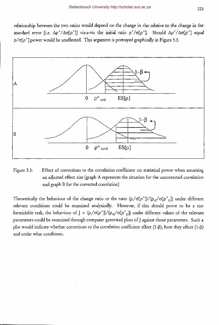
223
relationship between the two ratios would depend on the change in rho relative to the change in the
standard error [i.e. ~p"/ ~cr[p"]] vis-a-vis the initial ratio p" /cr[p"]. Should ~p" I ~cr[p"] equal
p/ cr[p "]power would be unaffected. This argument is portrayed graphically in Figure 5.3.
A
B
Figure 5.3:
0 P" crit
0 PI\ . cent
ES[p]
ES[p]
Effect of corrections to the correlation coefficient on statistical power when assuming
an adjusted effect size [graph A represents the situation for the uncorrected correlation
and graph B for the corrected correlation]
Theoretically the behaviour of the change ratio or the ratio (p/cr[p"])/(p1cfcr[p" cJ) under different
relevant conditions could be examined analytically. However, if this should prove to be a too
formidable task, the behaviour of J = (p/cr[p"])/(p1cfcr[p" cJ) under different values of the relevant
parameters could be examined through computer generated plots of J against those parameters. Such a
plot would indicate whether corrections to the correlation coefficient affect (1-~), how they affect (1-~)
and under what conditions.
Stellenbosch University http://scholar.sun.ac.za
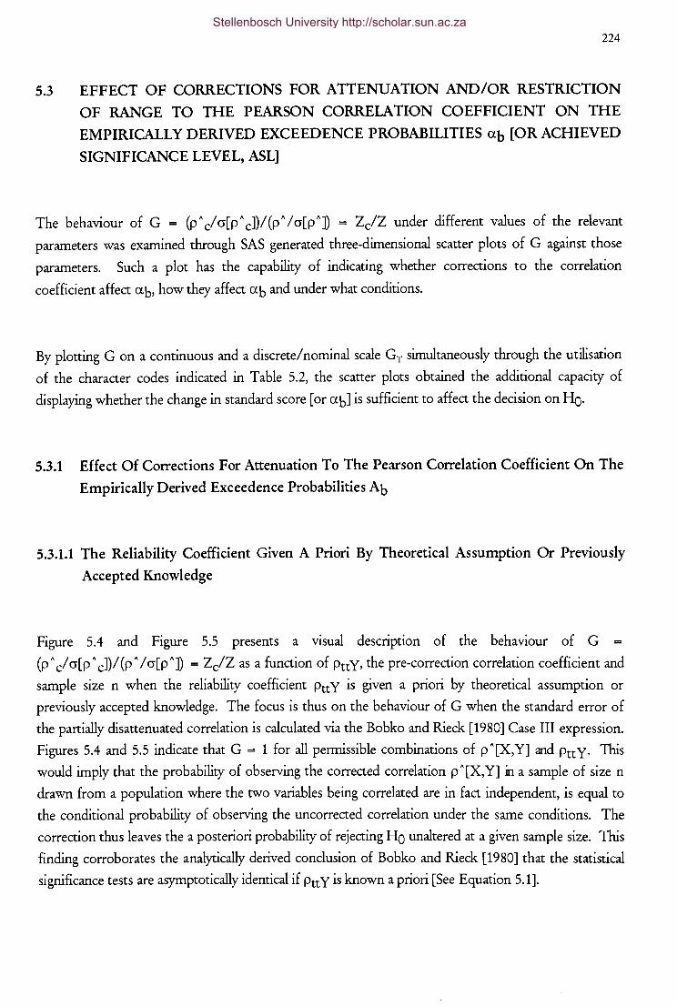
224
5.3 EFFECT OF CORRECTIONS FOR ATTENUATION AND/OR RESTRICTION
OF RANGE TO THE PEARSON CORRELATION COEFFICIENT ON THE
EMPIRICALLY DERIVED EXCEEDENCE PROBABILITIES a.b [OR ACHIEVED
SIGNIFICANCE LEVEL, ASL]
The behaviour of G = (pA clcr[pA c])/(pA /cr[pA]) = ZcfZ under different values of the relevant
parameters was examined through SAS generated three-dimensional scatter plots of G against those
parameters. Such a plot has the capability of indicating whether corrections to the correlation
coefficient affect a.b, how they affect a.b and under what conditions.
By plotting G on a continuous and a discrete/ nominal scale GT simultaneously through the utilisation
of the character codes indicated in Table 5.2, the scatter plots obtained the additional capacity of
displaying whether the change in standard score [or ab] is sufficient to affect the decision on Ho.
5.3.1 Effect Of Corrections For Attenuation To The Pearson Correlation Coefficient On The
Empirically Derived Exceedence Probabilities Ab
5.3.1.1 The Reliability Coefficient Given A Priori By Theoretical Assumption Or Previously
Accepted Knowledge
Figure 5.4 and Figure 5.5 presents a visual description of the behaviour of G =
(pA clcr[pA c])/(pA /cr[pA]) = ZcfZ as a function of PttY' the pre-correction correlation coefficient and
sample size n when the reliability coefficient Ptt y is given a priori by theoretical assumption or
previously accepted knowledge. The focus is thus on the behaviour of G when the standard error of
the partially disattenuated correlation is calculated via the Bobko and Rieck [1980] Case III expression.
Figures 5.4 and 5.5 indicate that G = 1 for all permissible combinations of pA[X,Y] and PttY· This
would imply that the probability of observing the corrected correlation pA[X,Y] in a sample of size n
drawn from a population where the two variables being correlated are in fact independent, is equal to
the conditional probability of observing the uncorrected correlation under the same conditions. The
correction thus leaves the a posteriori probability of rejecting Ho unaltered at a given sample size. This
finding corroborates the analytically derived conclusion of Bobko and Rieck [1980] that the statistical
significance tests are asymptotically identical if PttY is known a priori [See Equation 5.1].
Stellenbosch University http://scholar.sun.ac.za

Figure 5.4:
Figure 5.5:
225
0.920
0.100 0.040
G = (pA clcr[pA cJ)/(pA /cr[pA]) = ZciZ as a function of PttY' the pre-correction
correlation coefficient and sample size n when the reliability coefficient PttY is given a
priori by theoretical assumption or previously accepted knowledge; n is fixed at 90
0.920
0.627
RXY
0.100 0.040
G = (pA clcr[pA cJ)/(pA /cr[pA]) = ZcfZ as a function of PttY' the pre-correction
correlation coefficient and sample size n when the reliability coefficient PttY is given a
priori by theoretical assumption or previously accepted knowledge; n is fixed at 120
Stellenbosch University http://scholar.sun.ac.za

226
G = (pA clcr[pA cJ)/(pA /cr[pA])
= (p A cl cr[p A d) ( cr[p A]/ p A) ------------------------------- ------------ 5.1.1
Substituting Equation 4.13 and Equation 3.2 in Equation 5.1.1
G = ((p A /~PttY)(1/ cr[p A cJ)((1-p A 2)/~n)(1/ p A]}-------------------------------------------- 5.1.2
Canceling out the term p A and substituting Equation 4.25 in Equation 5.1.2:
G = (11 ~ Ptt y) (1/ (1/ ~n) ( 1/ ~ Ptt y) ( 1-p A 2)) ( ( 1-p A 2)/ ~n) ------------------------------------------------ 5.1.3
Simplifying Equation 5.1.3:
G = (li~PttY)(~n)(~PttY)(1/(1-pA 2))((1-pA 2)/~n) = 1----------------------------------------------------------------------------------------------------------------------------- 5. 1
Therefore it follows that Zc = Z.
5.3.1.2 The Reliability Coefficient Obtained From An Independent Data Set
Figures 5.6 - 5.9 depict the reaction of G to changes in the initial obtained correlation coefficient,
reliability coefficient and sample size when the reliability is obtained from an independent data set. The
focus is thus on the behaviour of G when the standard error of the partially disattenuated correlation is
calculated via the Bobko &Rieck [1980] Case II expression. Figures 5.6- 5.9 indicate that G < 1 for all permissible combinations of p A [X,Y] and Ptt y and for all values of n. This would imply that the
probability of observing the corrected correlation p A c in a sample of size n drawn from a population
where the two variables being correlated are in fact independent, is consistently greater than the
conditional probability of observing the uncorrected correlation under the same conditions. The
correction thus reduces the a posteriori probability of rejecting Ho for a given sample size. The
increase in ab produced by the correction for attenuation has the effect of changing some significant
uncorrected correlations into insignificant partially disattenuated correlations. If the three dimensional
plots are rotated to provide a view from the pA[X,Y] axis, the region in which the correction changes
the significance test outcome can be seen more clearly. Figure 5.10 and Figure 5.11 suggest [see Table
5.2] the change in decision outcome to occur in a specific region on the pA[X,Y] axis, as a function of
sample size, for all values of PttY. As sample size increases the region shifts to lower values of
Stellenbosch University http://scholar.sun.ac.za

Figure 5.6:
Figure 5.7:
227
0.980
0. 72 8
0. 47 6 0.920
0.100 0.040
G = (p" clcr[p" cJ)/(p" /cr[p"]) = ZciZ as a function of PttY' the pre-correctiOn
correlation coefficient and sample size n when the reliability coefficient PttY is obtained
from an independent data set; n is fixed at 10
0 829
0. 6 16
0 402 0.920
0.333 RXY
0.100 0.040
G = (p"c/cr[p" cJ)/(p" /cr[p"]) = ZciZ as a function of PttY• the pre-correctiOn
correlation coefficient and sample size n when the reliability coefficient PttY is obtained
from an independent data set; n is fixed at 20
Stellenbosch University http://scholar.sun.ac.za

Figure 5.8:
Figure 5.9:
228
0.573
0. 425
0. 176 0.920
0.627
0.333 RXY
0.100 0.040
G = (p~ clcr[p~ cJ)/(p~ /cr[p~]) = ZciZ as a function of PttY• the pre-correct10n
correlation coefficient and sample size n when the reliability coefficient PttY is obtained
from an independent data set; n is fixed at 90
0. 53 4
0. g 2 0
0.627
0.333 RXY
G = (p~ clcr[p~ cJ)/(p~ /cr[p~]) = Zc!Z as a function of PttY• the pre-correctwn
correlation coefficient and sample size n when the reliability coefficient PttY is obtained
from an independent data set; n is fixed at 120
Stellenbosch University http://scholar.sun.ac.za

0.980
0. 728
0. 476
0. 224 0.900
0.633
RTIY
229
0.100 0.040 RXY
Figure 5.10: G = (pA cfcr[pA cJ)/(pA/cr[pA]) = ZcfZ as a function of PttY' the pre-correct10n
correlation coefficient and sample size n when the reliability coefficient PttY is obtained
from an independent data set [rotated]; n is fixed at 10
0.633
0. 470
0.307
o . 1 44 .LU+IlllmllllmHffirttttttttt 0.900
RTTY
0.100 0.040 RXY
Figure 5.11: G = (pA clcr[pA cJ)/(pA /cr[pA]) ZcfZ as a function of PttY' the pre-correct10n
correlation coefficient and sample size n when the reliability coefficient PttY is obtained
from an independent data set [rotated]; n is fixed at 60
Stellenbosch University http://scholar.sun.ac.za

230
p A [X,Y]. The negative effect of the correction for criterion unreliability also seems to increase as Ptt y
and p A [X,Y] increases.
Bobko and Rieck [1980, p. 393] analytically reach a similar, although less detailed, conclusion:
If however ryy is estimated independently of ryx, B is inherently positive. In this case rxTy is still larger than
rxy by a factor ryy·lh. However, S.E.(rxTy) has increased by a greater factor, since S.E.(rxTy)=(A+B)lh >
A Y2 = ryy·1hS.E.(ryx). Thus, z1 >zz and it is recommended that the uncorrected coefficient be used for
hypothesis testing, since it provides a more powerful test.
The latter recommendation should be challenged, however, since it implies that the one coefficient can
serve as a logical substitute for the other. As was argued earlier a choice between p A [X, Y] and
p A c[X,Y] makes no sense since both constitute meaningful but qualitatively different, although related,
quantities.
5.3.1.3 The Reliability Coefficient Obtained From The Same Data Set As p A [X, Y]
The reaction of G = (pA clcr[pA cJ)/(pA/cr[pA]) = ZciZ as a function of PttY' the pre-correction
correlation coefficient and sample size n when the reliability coefficient PttY is obtained from the same
sample as pA[X,Y], is graphically portrayed in Figures 5.12- 5.15. An alternative perspective is again
provided in Figure 5.16 and Figure 5.17 by rotating the plot towards the pA[X,Y] axis. The behaviour
of G when the standard error of the partially disattenuated correlation is calculated via the Bobko and
Rieck [1980] Case I expression, is very similar to its behaviour under Case II conditions. All the
conclusions that were deduced under paragraph 5.3.1.2 thus also apply to Case I conditions. These
findings seems to be in line with the thinking of Bobko and Rieck [1980, p. 393], while at the same time
offering a significantly more detailed and precise description of the effect of correcting the correlation
coefficient for attenuation:
Finally, if ryy and rxy are estimated from the same sample, then the ordinal relationship between S.E.(rxTy) =
(A+B-C)Ih and A lh = ryy·lhs.E.(rxy) is not clear because (B-C) may be either positive or negative. Given
that no interpretable pattern regarding the sign of (B-C) has been found, it is recommended that the
uncorrected coefficient be tested.
Stellenbosch University http://scholar.sun.ac.za

231
0.999
0. 7 4 2
0.484 0.920
0.100 0.040
Figure 5.12: G = (PAc/cr[pAcJ)/(pA/cr[pA]) = ZcfZ as a function of PttY' the pre-correctiOn
correlation coefficient and sample size n when the reliability coefficient PttY is obtained
from the same data set; n is fixed at 10
0 840
0. 6 2 4
0.407
0.920
0.627
0.333 RXY
0.100 0.040
Figure 5.13: G = (p A cl cr[p A cJ)/ (p A I cr[p A]) = ZcfZ as a function of PttY' the pre-correctiOn
correlation coefficient and sample size n when the reliability coefficient PttY is obtained
from an independent data set; n is fixed at 20
Stellenbosch University http://scholar.sun.ac.za

232
c
0. 5 71
0. 4 28
0 280 0.920
----0.627
0.333 RXY
0.100 0.040
Figure 5.14: G = (p" clcr[p" cJ)/(p" /cr[p"]) = ZciZ as a function of PttY' the pre-correct10n
correlation coefficient and sample size n when the reliability coefficient PttY is obtained
from an independent data set; n is fixed at 90
0. 537
0.920
0.627
0.333 RXY
Figure 5.15: G = (p" clcr[p" cJ)/(p" /cr[p"]) = Zc!Z as a function of PttY' the pre-correctwn
correlation coefficient and sample size n when the reliability coefficient PttY is obtained
from an independent data set; n is fixed at 120
Stellenbosch University http://scholar.sun.ac.za

0.840
0.624
0.407
0 19 1 0.90
0.633
Rl TY 0.367
0.1000.040
___ .. , ____ _ ----------'
RXY
Figure 5.16: G = (p~ clcr[p~ cJ)/(p~ /cr[p~]) = ZcfZ as a function of PttY' the pre-correctiOn
correlation coefficient and sample size n when the reliability coefficient PttY is obtained
from an independent data set [rotated]; n is fixed at 20
0. 5 77
0.428
0.280
0. 131 0.900
RTTY
0.100 0.040 RXY
Figure 5.17: G = (P~c/cr[p~cJ)/(p~ /cr[p~]) = Zc!Z as a function of PttY' the pre-correctiOn
correlation coefficient and sample size n when the reliability coefficient PttY is obtained
from an independent data set [rotated]; n is fixed at 90
Stellenbosch University http://scholar.sun.ac.za

234
5.3.2 Effect Of Corrections For Restriction Of Range To The Pearson Correlation Coefficient
On The Empirically Derived Exceedence Probabilities Ub
5.3.2.1 Case 2 [Case A] Restriction Of Range
Figures 5.18 - 5.21 depict the reaction of G to changes in the initial, obtained correlation coefficient
p A [ x,y ], the ratio K = cr[X]/ cr[ x] [and by implication, therefore, the selection ratio [ ~] since K =
[1+(zcA-/~)-(A-/~) 2J-1] and sample size n when the obtained correlation had been attenuated through
Case 2 [Case A] selection. Figures 5.18- 5.21 reveal that G ~ 1 for all combinations of pA[x,y], K and
n. ForK= 1, G logically equals unity since pA[x,y] = pA[X,Y] and cr(pA[x,y] = cr(pA[X,Y]). It thus
follows that for all combinations of n, pA[x,y] and K > 1, the probability of observing pA[x,y]
conditional on Ho: p[x,y] = 0 [i.e. ab ] is systematically bigger than the probability of observing the
corresponding corrected correlation coefficient conditional on the hypothesis that p[X, Y] = 0. Figures
5.18- 5.21 furthermore demonstrate that the effect of the Case 2 [Case A] correction for restriction of
range on ab intensifies curvilinearly as pA[x,y] and K increases. In addition, the decrease in Ub
produced by the correction for restriction of range has the effect of changing some insignificant
uncorrected correlations into significant corrected correlations [see Table 5.2]. This effect seems to be
relatively sensitive to sample size. At n ~ 120 Case 2 [Case A] restriction of range corrections to the
correlation coefficient no longer have the effect of changing the significance test outcome [given ac =
0.05]. Figures 5.18- 5.21 suggest the change in decision outcome to occur in a specific region on the
p A[X,Y] - K space as a function of sample size. As sample size increases, the region shifts to lower
values of pA[X,Y] but simultaneously also higher values of K [i.e. smaller/stricter selection ratios].
These findings are in agreement with the analytical conclusions reached by Bobko and Rieck [1980, p.
393] but simultaneously offering a significantly more detailed and precise description of the effect of
correcting the correlation coefficient for Case 2 [Case A] restriction of range:
Regarding the correlation corrected for restriction of range, Moran's test compares z3 = rrang/S.E.(r range)
to a standard normal distribution. Again letting z1 = r/S.E.(r), it is easily shown [See Equation 5.2] that
z3/z1 = [1+rl(K-1)] > 1 if K > 1. Thus the Moran test of a validity coefficient corrected for restriction in
range is asymptotically more powerful than the test of the uncorrected coefficient.
G = (p A cl cr[p A cJ)/(p A I cr[p A])
= (p A cl cr[p A cJ) ( cr[p A]/ p A) ----------------------------------------------------------------------------- 5 .2.1
Substituting the expression for the correlation corrected for Case 2 [Case A] restriction of range
[Equation 3.4] in Equation 5.2.1:
Stellenbosch University http://scholar.sun.ac.za

235
0.95
Figure 5.18: G = (PAc/cr[pA cJ)/(pA/cr[pA]) = ZcfZ under Case 2 [Case A] restriction of range as a
function of PnY and the pre-correction correlation coefficient for n fixed at 10
0.95
Figure 5.19: G = (pA clcr[pA cJ)/(p" /cr[p"]) = ZcfZ under Case 2 [Case A] restriction of range as a
function of PnY and the pre-correction correlation coefficient for n fixed at 20
Stellenbosch University http://scholar.sun.ac.za

236
0.95
Figure 5.20: G = (P~c/cr[p~ cJ)/(p~ /cr[p~]) = ZcfZ under Case 2 [Case A] restriction of range as a
function of Ptt y and the pre-correction correlation coefficient for n fixed at 90
0.95
Figure 5.21: G = (p~ clcr[p\J)/(p~/cr[p~]) = ZcfZ under Case 2 [Case A] restriction of range, as a
function of PttY and the pre-correction correlation coefficient for n fixed at 120
Stellenbosch University http://scholar.sun.ac.za

237
Canceling out the term p ~ and substituting Equation 4.35 and Equation 3.4 in Equation 5.2.2:
G = (K/(1-p ~2+ p ~2K2)'h)((1-p ~2+ p ~2K2)312/K)(l/ cr[p ~])(cr[p ~])
= ( 1-p ~ 2 + p ~ 2K 2) -------------· -------------------------------------------------------- 5.2
Therefore it follows from Equation 5.2 that:
ForK >1,G > 1
5.3.2.2 Case 3 [Case C] Restriction Of Range
The behaviour of Gunder changes of K, n, p~[x,y], p~[x,z] and p~[y,z], when the obtained correlation
had been attenuated by selection on a third variable Z, is depicted in Figures 5.22 - 5.27. An
examination of Figures 5.22- 5.27 firstly confirms the logically necessary conclusion that forK= 1, for
all permissible combinations of values of p~[x,y], p~[x,z], p~[y,z] and n, G = 1. Figures 5.22 - 5.27
furthermore indicate that forK> 1, G reacts to changes inK, n, p~[x,y], p~[x,z] and p~[y,z] -with
values greater than and less than 1. Correcting the correlation coefficient for Case C restriction of
range thus increases the conditional probability ab = P[p~ c ~ p~ cb I p~ c=O] relative to ab = P[p~ ~ P~b I p~=O] at some combinations of values of n, K [K > 1], p~[x,y], p~[x,z] and p~[y,z] [thereby
reducing the chances of rejecting Ho] while it decreases ab associated with the corrected coefficient
relative to ab associated with p~ in other regions of the six dimensional space [thereby increasing the
chances of rejecting HoJ. These changes in Ub produced by the correction for restriction of range has
the effect of changing some insignificant uncorrected correlations into significant corrected correlations
and vice versa [see Table 5.2].
The region of change from insignificance to significance seems:
~ to occur at the lower end of the p~[x,y] axis for moderate to high p~[x,z] values;
~ to shift towards the upper end of the p ~ [ x,z] axis as p ~ [y ,z] increases;
~ to spread towards zero on the p ~ [ x,y] axis as K increases; and
~ to diminish as n increases.
In contrast, the region of change from significance to insignificance seems:
~ to occur at the lower end of the p~[x,z] axis for moderate to high p~[x,y] values;
~ to shift towards the upper end of the p ~ [ x,y] axis as p ~ [y ,z] increases;
~ to spread towards zero on the p~[x,z] axis asK decreases; and
Stellenbosch University http://scholar.sun.ac.za

238
0.920
Figure 5.22: G = (pAcfcr[pA cJ)/(pA /cr[pA]) = ZcfZ under Case 3[i] [Case C[i]]restriction of range
as a function of p A [ x,y] and p A [ x,z] for n fixed at 10, K fixed at 2 and p A [y ,z] fixed at
0.25
13 04
8. 7 1
4.38
0.05 0.92
0. 9 2 0
0.627
RXZ
0.040 0.040
Figure 5.23: G = (p A cl cr[p A cJ)/ (p A I cr[p A]) = ZcfZ under Case 3[i] [Case C[i]] restriction of range
as a function of pA[x,y] and pA[x,z] for n fixed at 10, K fixed at 4 and pA[y,z] fixed at
0.25
Stellenbosch University http://scholar.sun.ac.za

239
7.67
5. 18
0.920
0.040 0.040
Figure 5.24: G = (p A cl cr[p AcJ)/(p A I cr[p A]) = Zc!Z under Case 3[i] [Case C[i]] restriction of range
as a function of p A [ x,y] and p A [ x,z] for n fixed at 90, K fixed at 2 and p A [y ,z] fixed at
0.25
1 J. 04
8. 71
4 . J8 0.920
0.040 0.040
Figure 5.25: G = (pA clcr[pA cJ)/(pA /cr[pA]) = ZciZ under Case 3[i] [Case C[i]] restriction of range
as a function of p A [ x,y] and p A [x,z] for n fixed at 90, K fixed at 2 and p A [y ,z] fixed at
0.25
Stellenbosch University http://scholar.sun.ac.za

240
J.07
2.07
0.920
0.627
RXZ
Figure 5.26: G = (p A cl cr[p A cJ)I (p A I cr[p A]) = ZciZ under Case 3[i] [Case C[i]] restriction of range
as a function of pA[x,y] and pA[x,z] for n fixed at 60, K fixed at 4 and pA[y,z] fixed at
0.10
0.64
Figure 5.27: G = (p A cl cr[p A cJ)I (p A I cr[p A]) = ZciZ under Case 3[i] [Case C[i]] restriction of range
as a function of p A [x,y] and p A [ x,z] for n fixed at 60, K fixed at 4 and p A [y ,z] fixed at
0.75
Stellenbosch University http://scholar.sun.ac.za

241
);;;> to diminish as n increases.
The effect of corrections for Case 3[i] [Case qi] restriction of range thus seems somewhat more
complex than the effect of corrections for Case 2 [Case A] restriction of range. Inspection of Figures
5.22- 5.27 suggests the following additional specific conclusions on the effect of corrections for Case C
restriction of range to be appropriate:
);;;> G increases as K increases [i.e. as the selection ratio decreases or selection becomes
more severe];
);;;> for any K > 1, G increases as the correlation of the selection variable Z with the
predictor X increases;
);;;> for any K > 1, G increases as the correlation of the selection variable Z with the
criterion Y increases; and
);;;> for any K > 1, higher G values are found at extreme low values of p A[x,y];
5.3.3 Effect Of Corrections For Criterion Unreliability And Restriction Of Range To The
Pearson Correlation Coefficient On The Empirically Derived Exceedence Probabilities
<Xb
The reaction of G = (pA clcr[pAcJ)/(pA /cr[pA]) to changes in pA[x,y], K, nand PttY whn correcting
the obtained correlation coefficient for criterion unreliability and [Case 2 [Case A] restriction of range
simultaneously is depicted in Figures 5.28 - 5.35. Figures 5.28 -5.35 indicate G > 1 for K > 1 for all
values of pA[x,y] and PttY. Figure 5.28 and Figure 5.32 indicate G < 1 forK = 1 in a small region
defined by low values on both the Ptt y and p A [ x,y] axes.
It thus follows that for all combinations of n, pA[x,y], PttY and K > 1 the probability of observing
p A[x,y] conditional on Ho: p[x,y] = 0 [i.e. <Xb] is systematically bigger than the probability of observing
the corresponding double corrected correlation coefficient conditional on the hypothesis that p[X, Ty]
= 0. Figures 5.28 - 5.35 furthermore demonstrate that the effect of the double correction for [Case 2
[Case A]] restriction of range and criterion unreliability on <Xb intensifies [i.e. G increases] as pA[x,y]
and K increases and PttY decreases. In addition, the decrease in <Xb produced by the double correction
has the effect of changing some insignificant uncorrected correlations into significant corrected
correlations [see Table 5.2] when K > 1. ForK> 1 the opposite effect does not seem to occur. The
aforementioned effect seems to be relatively sensitive to sample size. At n ~ 120, double corrections to
the correlation coefficient no longer have the effect of changing the significance test outcome [given ac
= 0.05]. Figures 5.28- 5.35 suggest the change in decision outcome to occur in the lower region of the
p A[x,y] axis and the full range of PttY values as a function of sample size and K. As sample size
Stellenbosch University http://scholar.sun.ac.za

242
1 . 2 9 8
1 . 0 2 J
0. 747 0.95
RT TY 0.050 0.05
Figure 5.28: G = (p~cfcr[p~ cJ)/(pA /cr[p~]) as a function of p~[x,y] and PttY when correcting the
obtained correlation coefficient for criterion unreliability and [Case 2 [Case A]]
restriction of range simultaneously; n is fixed at 10 and K is fixed at 1
5.01
J.68
2. J4 0.95
0.65
RXY
RT TY 0.050 0.05
Figure 5.29: G = (p~ cfcr[p~cJ)/(p~/cr[p~]) as a function of p~[x,y] and PttY when correcting the
obtained correlation coefficient for criterion unreliability and [Case 2 [Case A]]
restriction of range simultaneously; n is fixed at 10 and K is fixed at 2
Stellenbosch University http://scholar.sun.ac.za

243
0.95
Figure 5.30: G = (p' clcr[p' cJ)/(p' /cr[p']) as a function of p'[x,y] and PttY when correcting the
obtained correlation coefficient for criterion unreliability and [Case 2 [Case A]]
restriction of range simultaneously; n is fixed at 10 and K is fixed at 3
0.95
0.65
0.35 RXY
Figure 5.31: G = (p' clcr[p' cJ)/(p' /cr[p']) as a function of p'[x,y] and PttY when correcting the
obtained correlation coefficient for criterion unreliability and [Case 2 [Case A]]
restriction of range simultaneously; n is fixed at 10 and K is fixed at 4
Stellenbosch University http://scholar.sun.ac.za

244
0.95
0.65
RXY
Figure 5.32: G = (p~ clcr[p~ cJ)/(p~ /cr[p~]) as a function of p~[x,y] and PttY when correcting the
obtained correlation coefficient for criterion unreliability and [Case 2 [Case A]]
restriction of range simultaneously; n is fixed at 120 and K is fixed at 1
0.95
0.65
RXY
Figure 5.33: G = (p~ clcr[p~ cJ)/(p~ /cr[p~]) as a function of p~[x,y] and PttY when correcting the
obtained correlation coefficient for criterion unreliability and [Case 2 [Case A]]
restriction of range simultaneously; n is fixed at 120 and K is fixed at 2
Stellenbosch University http://scholar.sun.ac.za

245
0.95
0.65
RXY
Figure 5.34: G = (pA clcr[pA cJ)/(pA /cr[pA]) as a function of pA[x,y] and PttY when correcting the
obtained correlation coefficient for criterion unreliability and [Case 2 [Case A]]
restriction of range simultaneously; n is fixed at 120 and K is fixed at 3
0.95
0.35 RXY
Figure 5.35: G = (pA clcr[pA cJ)/(pA /cr[pA]) as a function of pA[x,y] and PttY when correcting the
obtained correlation coefficient for criterion unreliability and [Case 2 [Case A]]
restriction of range simultaneously, n is fixed at 120, K is fixed at 4
Stellenbosch University http://scholar.sun.ac.za

246
increases the region shifts to lower values of pA[x,y]. As sample size increases the spread of the region
also seems to be restricted more and more to the lower regions of the rtty axis. The region tends to
increase at higher values of K [i.e. smaller I stricter selection ratios].
5.4 EFFECT OF CORRECTIONS FOR ATTENUATION AND/OR RESTRICTION
OF RANGE TO THE PEARSON CORRELATION COEFFICIENT ON THE A
PRIORI PROBABILITIES [1-p] OR POWER OF THE TESTS OF H0.
Previously is was argued that the effect of corrections to the correlation coefficient for the attenuating
effect of restriction of range and/ or criterion unreliability on statistical power would depend on how
the ratio p A I cr[p A] compares to the ratio p A cf cr[p A cJ. The critical ratio is thus
(pA/cr[pA])/(pAc/cr[pAcJ). Specifically it was argued that if (pA/cr[pAJ)/(pAc/cr[pAcJ) should equal
unity, the power of the test of the hypothesis Ho: p = 0 would equal the power of the test of the
hypothesis Ho=Pc = 0. If, however, (pA /cr[pA])/(pA clcr[pA cJ) should drop below 1, power would be
positively affected since it would imply that the critical cutoff under Ho would translate to a more
extreme standard score under Ha for the corrected correlation coefficient than for the uncorrected
coefficient. It thus follows that if Pc = p, J necessarily would be greater than one since cr[ r] < cr[ A J All corrections to the correlation coefficient would consequently affect statistical power negatively. If, however, Pc > p, the previous argument no longer applies.
The behaviour of the ratio (pA /cr[pA])/(pA clcr[pA cJ) under different relevant conditions was
consequently examined analytically when Pc assumed under Ha is estimated via the appropriate
correction formula from p assumed under Ha. In cases where this failed to provide an unambiguous
indication of the effect of the particular correction on statistical power, the behaviour of J =
(pA /cr[pA])/(pA clcr[pA cJ) under different values of the relevant parameters was simulated and
examined through SAS generated three-dimensional scatter plots of J against those parameters. These
plots would indicate whether corrections to the correlation coefficient affect (1-p), how they affect (1-
P) and under what conditions.
Stellenbosch University http://scholar.sun.ac.za

247
5.4.1 Effect Of Corrections For Attenuation To The Pearson Correlation Coefficient On The
A Priori Probabilities [1-P] Or Power Of The Tests Of Ho.
5.4.1.1 The Reliability Coefficient Given A Priori By Theoretical Assumption Or Previously
Accepted Knowledge
The asymptotic standard error for the partially disattenua~ed correlation coefficient derived by Bobko
and Rieck [1980] for Case III conditions is used to analytically argue as follow:
J = (p A I cr[p A])/ (p A cl cr[p A cJ) = (p A I cr[ p A ]) ( cr[ p A cJ/ p A c) ----------------------------------------------------------------------------------------- 5. 3 .1
Substituting the expression for the partially attenuated validity coefficient [Equation 3.2] in Equation
5.3.1:
J = (pA /cr[pA])(cr[pAcJ)/(pA /-.Jptty) = (p A I cr[ p A]) ( cr[p A cJ) ( -.J Ptt yIp A}----------------------------------------------------------------- 5.3 .2
Substituting the expression for the standard error of the uncorrected correlation coefficient [Equation
4.13] in Equation 5.3.2:
J = (pA /(1-pA2)/-.Jn)(cr[pA cJ)(-.Jptty/pA) = (p A) ( -.J n/ ( 1-p A 2)) ( cr[p A cJ) ( -.J Ptt yIp A) ---------------------------~------------------------------------- 5. 3. 3
Substituting Bobko and Rieck's Case III expression for the standard error of the corrected correlation
coefficient [Equation 4.25] in Equation 5.3.3:
J = (p A) (-.Jn/ (1-p A 2)) (li-.Jn)(1/-.Jptty)(1-p A2)(-.Jptty/ p A)------------------------------------------------- 5.3.4
Therefore:
J = (p A I cr[p A])/ (p A cl cr[p A cJ) = 1---------------------------------------------------------------------- 5.3
Equation 5.3 thus leads to the result that the power of the statistical significance test will, under the
conditions assumed, remain unaffected by the correction for attenuation for the criterion unreliability
only.
Stellenbosch University http://scholar.sun.ac.za

248
5.4.1.2 The Reliability Coefficient Obtained From An Independent Sample
The asymptotic standard error for the partially disattenuated correlation coefficient derived by Bobko
and Rieck [1980] for Case II conditions is used to analytically argue as follow:
J = (p" /cr[p"])/(p" clcr[p" cJ)
= (p "I cr[p "]) ( cr[p "cJI p "c) --------------------------------------------------- 5.4 .1
Substituting the expression for the partially attenuated validity coefficient [Equation 3.2] in Equation
5.4.1 and canceling out the term p":
J = (p" /cr[p"])(cr[p" cJ)/(p" /..Jp" ttY)
= (p "I cr[p "])(cr[p "cJ)(..Jp "ttY/ p ") = ( 11 cr[ p " ]) ( ..J p " tty) ( cr[ p " cJ) ----------------------------------------------------------------------------------------- 5 .4. 2
Substituting the expression for the standard error of the uncorrected correlation coefficient [Equation
4.13] in Equation 5.4.2:
J = (1/(1-p" 2)/..Jn)(..Jp"tty)(cr[p" cJ) = ( ..J nl ( 1-p " 2) ( ..J p "tty) ( cr[ p " cJ)------------------------------------------------------------------------------------- 5 .4. 3
Substituting Bobko and Rieck's Case II expression for the asymptotic standard error for the partially
disattenuated correlation coefficient [Equation 4.24] in Equation 5.4.3:
J = (..Jn/(1-p"2)(..Jp" ttY){(1/n)(llp" ttY)(1-p"2)2+
(1/4) (1/ n) (1/ p "ttY3)(p "2)(1-p "tty2)2} 1h -------------------------------------------------------- 5.4.4
Squaring Equation 5.4.4 and canceling out terms:
J2 = (n/(1-p "2)2(p "ttY){ (1/n)(1/ p "ttY)(1-p "2)2+ (1/ 4)(1/ n)(ll p "ttY3)(p "2)(1-p "ny2)2}
= { 1 + (1/ 4)(1/ p "ttY2)(p "2)(1-p "ttY2)2(1/ (1-p "2)2}
= {1 + (1/4)(p"2/(1-p"2)2)((1-p" ttY2)2/p" ttY2)}
= { 1 + (ll4)(p "I (1-p "2))2((1-p "ttY2)/ p "ttY)2}------------------------------------------------------- 5.4.5
Therefore:
J2 = (p "2 I cr[p "])2 I (p "cl cr[p" cJ)2 2:: 1------------------------------------------------------------------------ 5. 4.6
Stellenbosch University http://scholar.sun.ac.za

249
Since in Equation 5.4:
(11 4)(p" 1(1-p "2))2((1-p "ttY2)1 p" nY)2 must be> 0
Therefore:
J = (p "I cr[p "])I (p "cl cr[p "cJ) ~ 1----------------------------------------------------------- 5. 4
It thus follows that power is negatively affected by Case II corrections for criterion unreliability since
Equation 5.4 implies that the critical cutoff under Ho would translate to a less extreme standard score
under Ha for the corrected correlation coefficient than for the uncorrected coefficient.
5.4.1.3 The Reliability Coefficient Obtained From The Same Sample As p" [X, Y]
The asymptotic standard error for the partially disattenuated correlation coefficient derived by Bobko
and Rieck [1980] for Case I conditions is used to analytically argue as follow:
J = (p" lcr[p"])l(p"clcr[p" cJ) = (p " I cr[ p " ]) ( cr[ p " cJ I p " c) ------------------------------------------------------------------------------------------ 5. 5 .1
Substituting Equation 5.4.3 in Equation 5.5.1:
J = (-.fnl ( 1-p "2) ( .Y p "tty) ( cr[p "cJ) -------------------------------------------------------------------------- 5. 5.2
Squaring Equation 5.5.2:
F = (nl ( 1-p "2)2 (p "tty) ( cr2[ p "cJ)------------------------------------------------------------------------- 5. 5. 3
Substituting Bobko and Rieck's Case I expression for the asymptotic standard error for the partially
disattenuated correlation coefficient [Equation 4.23] in Equation 5.4.3:
F = {1 + (114)(p"l(1-p"2))2((1-p"tty2)lp"ny)2} + (nl(1-p "2)2(p "ttY){ (1ln)(ll P "ttY2)(p ')[(p "nY)(1-2p "2)-(.5)(p "2)(1-2p "2-p "tt y2)]}
= {1 + (114)(p" 1(1-p"2))2((1-p"tty2)lp" nY)2} +
(p "I (1-p "2)2) (11 p "tt y)[(p "nY)(1-2p "2)-(.5) (p "2) (1-2p "2-p "ttY2)]}---------------------------5.5
Stellenbosch University http://scholar.sun.ac.za

250
Equation 5.5, although it could be simplified further, fails to provide an unambiguous indication of the
effect of the [Case I] correction for criterion unreliability on statistical power. The reaction of J =
(pA 2/cr[pA])/(pA clcr[pA cJ) to changes in pA[X,Y], n and P\tY was subsequently calculated and
examined through SAS generated three-dimensional scatter plots of J against those parameters. Figure
5.36 and Figure 5.37 suggest Case 1 partial corrections for attenuation to negatively affect statistical
power for all permissible combinations of pA[X,Y] and pAttY and values of n. J is consistently greater
than 1 which implies that the critical cutoff under Ho translates to a less extreme standard score under
Ha for the corrected correlation coefficient than for the uncorrected coefficient. Figures 5.36 and 5.37
furthermore reveal that the negative effect of Case I partial corrections for attenuation on statistical
power increases curvilinearly with increases in the effect size assumed for the uncorrected correlation
coefficient over all levels of criterion reliability.
5.4.2 Effect Of Corrections For Restriction Of Range To The Pearson Correlation Coefficient
On The A Priori Probabilities [1-~] Or Power Of The Tests Of Ho.
5.4.2.1 Case 2 [Case A] Restriction Of Range
The asymptotic standard error for the correlation coefficient corrected for Case 2 [Case A] restriction
of range, derived by Bobko and Rieck [1980], is used to analytically argue as follow:
J = (p A I cr[p A])/ (p A cl cr[p A cJ) = (p A I cr[ p A]) ( cr[ p A cJ/ p A c) --------------------------------------------------------------------------------- 5. 6.1
Substituting the expression for the asymptotic standard error for the correlation coefficient corrected
for Case 2 [Case A] restriction of range, derived by Bobko and Rieck [1980] [Equation 4.35]
J = (p 'I cr[p A])(K/ (1 + p A 2K2-p ' 2)312)(cr[p A]) (1/ p A c)----------------------------------------------------5.6.2
Substituting the correction formula for Case 2 [Case A] restriction of range [Equation 3.4] in Equation
5.6.2:
J = (p A)(K/ (1 + p A2K2-p A2)312)((1 +p A2K2-p A2) 1h I p 'K)
= ( 1 + p A 2 K 2-p A 2) -1 ---------------------------------------------------------------------------------------------- 5. 6
Stellenbosch University http://scholar.sun.ac.za

251
0.920
0.627
RXY
Figure 5.36: J = (p • 2/ cr[p •])/(p • cl cr[p • cJ) as a function of p •[X,Y] and p • ttY for n fixed at 10
0.920
0. 6 2 7
O.JJJ RXY
Stellenbosch University http://scholar.sun.ac.za

252
Therefore it follows that:
and
It thus follows that the power of the statistical significance test would increase, should the correction
for Case 2 [Case A] restriction of range be applied to the observed, restricted correlation coefficient and
the uncorrected effect size estimate.
5.4.2.2 Case C Restriction Of Range
The asymptotic standard error for the correlation coefficient corrected for Case C restriction of range,
derived by Allen and Dunbar [1990], is sufficiently complex to eliminate, for all practical purposes, any
possibility of finding an analytical solution to the question in hand. Values of J were thus calculated for
changes in pA[x,z], pA[y,z], nand the initial uncorrected effect size estimate pA[x,y]. Figures 5.38- 5.43
provide a pictorial representation of the reaction of J to changes in pA[x,z], pA[y,z], nand pA[x,y].
Figures 5.38 - 5.43 suggest that Case C corrections for restriction of range can affect the statistical
power of significance tests both positively and negatively depending on the applicable parameter
settings. Corrections for Case C restriction of range [fortunately] seem to have maximum adverse
impact on statistical power when pA[x,y] is high and pA[x,z] and pA[y,z] is low. K seems to affect
power by aggravating the effect of the aforementioned parameters as K increases [i.e. as the selection
ratio decreases]. In contrast, corrections for Case C restriction of range seem to have maximum
beneficial impact on statistical power under those conditions where Case C restriction of range
corrections have their greatest impact, namely when pA[x,y] is low and pA[x,z] and pA[y,z] is high. K
again seems to affect power by aggravating the effect of the aforementioned parameters as K increases
[i.e. as the selection ratio decreases].
Stellenbosch University http://scholar.sun.ac.za

253
0.920
Figure 5.38: J = (pA/cr[pA])/(pAc/cr[pAcJ) under Case 3[i] [Case C[i]] restriction of range as a
function of pA[x,z] and pA[x,y] for n ftxed at 10, K fixed at 4 and pA[y,z]fixed at 0.25
19 10
12 7 6
6.42
0.08 0 920
0.920
RXZ
RXY
Figure 5.39: J = (pA /cr[pA])/(pA clcr[pA cJ) under Case 3[i] [Case C[i]] restriction of range as a
function of p A [ x,z] and p A [ x,y] for n fixed at 90, K fixed at 4 and p A [y ,z] ftxed at 0.25
Stellenbosch University http://scholar.sun.ac.za

254
3 96
2. 72
1.48 .920
0.040 0.040
Figure 5.40: J = (p A I cr[p A])/ (p A cl cr[p A cJ) under Case 3[i] [Case C[i]] restriction of range as a
function of pA[x,z] and pA[x,y] for n fixed at 90, K fixed at 2 and pA[y,z] fixed at 0.15
3.64
243
1 . 2 3 0. 7 2 0
RXZ
RXY 0.040 0.040
Figure 5.41: J = (pA /cr[pA])/(pA clcr[pA cJ) under Case 3[i] [Case C[i]] restriction of range as a
function of pA[x,z] and pA[x,y] for n fixed at 90, K fixed at 2 and pA[y,z] fixed at 0.65
Stellenbosch University http://scholar.sun.ac.za

255
0. g 20
Figure 5.42: J = (p~ /cr[p~])/(p~ cfcr[p~ cJ) under Case 3[i] [Case C[i]] restriction of range as a
function of p~[x,z] and p~[x,y] for n ft.xed at 90, K fixed at 4 and p~[y,z] fixed at 0.15
0. 7 2 0
Figure 5.43: J = (p ~I cr[p ~])/ (p ~ cl cr[p ~ cJ) under Case 3[i] [Case C[i]] restriction of range as a
function of p~[x,z] and p~[x,y] for n fixed at 90, K fixed at 4 and p~[y,z] fixed at 0.65
Stellenbosch University http://scholar.sun.ac.za

256
5.4.3 Effect Of Double Corrections For Attenuation And Restriction Of Range To The
Pearson Correlation Coefficient On The A Priori Probabilities [1-P] Or Power Of The
Tests OfHo.
Substituting the asymptotic standard error for the correlation coefficient double corrected for [Case 2
[Case A]] restriction of range and criterion unreliability derived by Bobko [1983] in J and analytically
simplifying the ratio would unlikely yield any definitive conclusion on the reaction of J to changes in the
initial uncorrected effect size estimate, n, ptt Y and K. The computational solution of J to changes in
the relevant parameters combined with pertinent three dimensional scatter plots once more seems to be
the more productive option. Figures 5.44- 5.47 depict the reaction of J to changes in the uncorrected
ES estimate, PttY, nand K. Figures 5.44- 5.47 reveal that the probability of the corrected correlation
coefficient exceeding the critical cut off correlation, conditional on a specific value for rho assumed
under Ha, is smaller than the corresponding conditional probability for the double corrected correlation
coefficient for all p A[x,y], PttY and forK> 1. Since J < 1 for all p A[x,y ], PttY and forK> 1, statistical
power is improved by the double correction for restriction of range and criterion unreliability, provided
the uncorrected ES estimate is also corrected via the appropriate correction formula [Equation 3.10 or
Equation 3.13] to obtain the corrected ES estimate. Maximum power benefits are obtained by the
double correction when pA[x,y] is high [i.e. the initial ES estimate is high], PttY is low and K is high [i.e.
the selection ratio is small]. Although n affects power, it does not seem to affect the change in power
brought about by the double correction to the correlation coefficient
5.5 SUMMARY
Chapter 5 presented an introductory synopsis of the basic logic underlying classical/Fisherian statistical
hypothesis/ significance testing.
The consequences of corrections for attenuation and/ or restriction of range to the Pearson correlation
coefficient on decisions on the validity of statistical null hypotheses were subsequently examined. Two
quantities were identified to have particular relevance, namely the empirically derived exceedence
probabilities and the power of the tests of Ho. The quantities G = (pA clcr[pA cJ)/(pA /cr[pA]) and J =
(p/ cr[p A])/ (Pre/ cr[p A cJ) were defined and shown to constitute appropriate indicators of the effect of
the corrections on ab and 1-p. The reaction of the ratios G and J to corrections to the validity
coefficient were examined analytically where possible. However, in cases where this proved to be a too
formidable task, the behaviour of G and J under different values of the relevant parameters was
examined through computer generated plots of G and J against those parameters.
Stellenbosch University http://scholar.sun.ac.za

257
0.993
0.728
0. 4 6 4
0 . 2 0 0 ~IRH+Ifttltttttttt 1. 0 00
0.6
R TTY 0.36
Figure 5.44: J = (p~ lcr[p~])l(p~ clcr[p~ cJ) under the joint correction for Case 2 [Case A] restriction
of range and criterion unreliability as a function of the initial uncorrected effect size
estimate and PttY for n fixed at 10 and K fixed at 2
0.993
0.728
0.464
0 . 2 0 0 .llmlmH!mftttttttttut 1. 00
0.683
Rl TY 0.367
0.0500.05
Figure 5.45: J = (p ~I cr[p ~])I (p ~ cl cr[p ~ cJ) under the joint correction for Case 2 [Case A] restriction
of range and criterion unreliability as a function of the initial uncorrected effect size
estimate and Ptt y for n fixed at 90 and K fixed at 2
Stellenbosch University http://scholar.sun.ac.za

258
0.050 0.05 RXY
Figure 5.46: J = (p~ /cr[p~])/(p~ clcr[p~ cJ) under the joint correction for Case 2 [Case A] restriction
of range and criterion unreliability as a function of the initial uncorrected effect size
estimate and PttY for n fixed at 10 and K fixed at 4
0 964
0.659
0.355
0.050 1. 0 00
0.683
RTTY 0.367
Figure 5.47: J = (p~ /cr[p~J)/(p~ clcr[p~cJ) under the joint correction for Case 2 [Case A] restriction
of range and criterion unreliability as a function of the initial uncorrected effect size
estimate and PttY for n fixed at 90 and K fixed at 4
Stellenbosch University http://scholar.sun.ac.za

CHAPTER6
EFFECT OF STATISTICAL CORRECTIONS TO THE VALIDITY COEFFICIENT ON
THE PARAMETERS OF THE DECISION FUNCTION
The purpose of the following discussion is to extend the logic underlying the corrections for restriction
of range and/ or criterion unreliability applied to the validity coefficient to the decision rule in terms of
which applicants are screened for employment and to examine the consequences of applying such
correction for actual selection decision making. A synopsis of the logic underlying selection decision
making will, however, first be presented so as to establish the necessary theoretical foundation for the
subsequent analysis.
6.1 THE DECISION FUNCTION IN PERSONNEL SELECTION
Personnel selection is necessitated by the combined effect of inter-individual differences amongst
applicants on those attributes that would determine their eventual job performance and the selecting
organisation's desire to maximise performance. The desire to maximise performance implies work
success as the ultimate/ final institutional criterion in terms of which applicants for employment should
ideally be evaluated and on which they should ideally be compared so as to arrive at an institutionally
rational selection decision. Personnel selection is, however, complicated by the obvious fact that
information on the ultimate institutional criterion can never be available at the time of the selection
decision. The only solution to this dilemma, apart from reducing selection to random assignment, is to
base the decision on relevant substitute information that is assessable prior to the selection decision.
Even if no direct information on the criterion ever enters the selection decision making process, the
criterion nonetheless always remains the focus of interest in selection assessment. This seemingly
innocent and too often forgotten fact, moreover, has significant implications for the interpretation and
evaluation of information entering the selection decision.
Only two basic options exist in terms of which such substitute information can be generated. In terms
of the first option substitute information would be obtained through low or high fidelity simulations of
the job content [or key performance areas] developed from systematically constructed job descriptions.
The first option thus requires no understanding of the reasons underlying differences in performance.
It does, however, require an understanding of the demands that collectively constitute the job. It in
essence argues that if the simulation would succeed in creating conditions that place similar demands
on people as the job would [although those conditions need not look similar to the job content],
measurements of performance in the simulation should be systematically related to eventual job
Stellenbosch University http://scholar.sun.ac.za

260
performance. Although the simulation should, under the aforementioned assumptions, logically invoke
the same attributes [or competencies] as would be required to succeed in the job, those critical
attributes and their interaction need not necessarily be understood. The second option, in contrast,
requires that the same job description should be examined again, but now with the explicit purpose of
inferring those qualities of job incumbents that are required to succeed in the job. The second option
thus requires a comprehensive understanding of the reasons underlying performance in addition to
clarity on the fundamental nature of the key performance areas comprising the job. It in essence argues
that if the hypotheses on job performance derived from the job description would be valid [i.e. if the
attributes suggested by the job description to be critical for success, are in fact competencies],
measurements of these critical characteristics [if combined in accordance with the dynamics of the
performance theory] should be systematically related to eventual job performance.
Information obtained via either one of the aforementioned two options derives it ability to act as a
substitute and thereby its relevance through the extent to which it correlates with a valid representation
or operationalisation of the ultimate criterion [i.e. to the extent that the substitute statistically explains
variance in the criterion]. This has the important [but seemingly too easily forgotten] implication that
any measurement procedure [interpreted in the widest possible meaning of the term] which delivers
[content/ construct valid] measurements of any knowledge domain, skill, ability, personality trait,
motive or style, but which bases its claim to relevance solely on logic, will remain on the level of
conjecture until empirically proven otherwise. Stated differently, attributes/ characteristics do not
qualify as competencies simply because they are designated as such. Competencies are underlying
characteristics of people [or behaviour] that have been empirically shm.m to be [causally] related to
effective job performance [Boyatzis, 1982; Spangenberg, 1990].
Relevance thus implies a systematic relationship between the criterion and the substitute information.
The identification of relevant substitute information therefore, by definition, creates the possibility of
estimating the expected criterion performance and/ or probability of success/ failure conditional on the
information content. One should in fact argue that the foregoing interpretation of the term relevance
flows logically from the need to predict the criterion on which the selection decision ideally should be
based, but which is not directly assessable at the time of the decision. A necessary prerequisite,
however, to achieve such criterion referenced interpretation of the substitute information, is that the
nature of the relationship between the substitute information and the criterion be known.
Effective [although not necessarily efficient] personnel selection is therefore possible if, and only if:
);> [substitute] information is available at the time of the selection decision that is
systematically related to the ultimate/final criterion of work success [i.e. relevant
information]; and
Stellenbosch University http://scholar.sun.ac.za

261
~ the nature of the relationship is at least subjectively/ clinically but preferably
statistically I actuarially] understood.
The relevance of substitute information is established through an extensive validation study as a form
of applied explanatory research [Ellis & Blustein, 1991; Landy, 1986; Schmitt & Landy, 1993]. The
credibility of the any claims to relevance resulting from a validation study will consequently in the final
analysis depend on the unassailableness, scientific rationality or validity [Cook, Campbell & Perrachio,
1991] of the research methodology through which hypotheses derived from a job description were
investigated.
Once the case for the relevance of the substitute information has been successfully argued, the question
on how to combine such information to arrive at a decision arises [strictly speaking, however, these two
issues can not be completely separated]. Two, and only two, basic option exist in terms of which
information can be combined for decision making. Both options require that the nature of the
relationship between the criterion and the substitute information be understood. The two options,
however, differ in the way they express their understanding of the criterion - information relationship.
The first option could be termed a judgmental, subjective or clinical mode of information combination
since the decision outcome is derived from human judgement based on an inexplicit and
unstandardised decision rule. The second option could be termed a mechanical, statistical or actuarial
mode of information combination since an explicit and standardised rule or formula dictates the
decision outcome [Gatewood & Feild, 1994]. Within the mechanical option a number of different
actuarial selection strategies can be distinguished. A selection strategy in the current context refers to
an explicit rule which determines, conditional on obtained information, the assignment of applicants to
one of three possible outcomes, namely terminal rejection, acceptation or further investigation
[Cronbach & Gieser, 1965; Gatewood & Feild, 1994]. All actuarial [i.e. prescriptive] selection strategies
can be reduced to a strategy matrix [Cronbach & Gieser, 1965] expressing its allocation of applicants to
treatments in terms of probabilities, restricted to either 0 or 1, conditional on obtained information.
The nature of a selection strategy and thus the structure of the strategy matrix depends on:
~ whether compensation will be permitted in the combination of information; and
~ whether multi-stage sequential assessment will be permitted or required.
The first consideration impacts on the number of ways [Coxon, 1982; Schiffman, Reynolds & Young,
1981] the strategy matrix contains. If an information x decision format is assumed for the most basic
strategy matrix, such a matrix would comprise two ways. If compensation is allowed, the strategy
matrix will always comprise two ways. The information way can be presented in terms of k class
intervals or in terms of a continuum. If compensation in the combination of information is disallowed,
the number of ways will increase from two to the number of dimensions information was obtained on.
Multi-stage assessment will affect the number of columns in the decision way of the strategy matrix and
Stellenbosch University http://scholar.sun.ac.za

262
the number of matrixes. Sequential assessment will result in an array of information x decision strategy
matrixes, each consisting of three columns in the decision way, except in the final matrix.
The content of the strategy matrix [i.e. the distribution of the conditional probabilities of acceptance
(either 0 or 1)], in tum will depend on:
~ whether quotas are in force;
~ the aspiration level of the decision maker;
~ the relevance of the information on which the strategy is based;
~ the nature of the relationship between the criterion and the selection information;
~ the presence of group x information interaction effects; and
~ the size of the applicant group;
The following [actuarial] selection strategies are typically distinguished [Gatewood & Feild, 1994;
Milkovich & Boudreau, 1994 ]:
~ regression strategy [single stage; compensation allowed]
~ multiple cutoff [single stage; limited compensation allowed]
~ multiple hurdle [multi-stage; no compensation allowed];
~ profile comparison [single stage; compensation depending on companson
technique]
~ combinations of the above.
Attention will henceforth solely be focused on the regression strategy. Three basic reasons motivated
the decision to restrict the analysis to the regression strategy only. To consider all the aforementioned
strategies in the current study was, firstly, considered unnecessarily ambitious. Although all the
selection strategies are worthy of consideration, they need not all be examined simultaneously in a
single study. The present study, secondly, chose to focus on the regression strategy because it forms
the implicit basis of all the other selection strategies and because it constitutes the strategy explicitly
assumed in the Brogden-Cronbach-Gleser utility analysis [Boudreau, 1991] and the Cleary-madel on
selection fairness [Cleary, 1968]. The goal of the multiple regression strategy is to find a weighted linear
combination of the individual information sources that minimises the sum of the squared deviations
between the linear combination and the actual criterion and thus that maximally correlates with the
actual criterion [Cohen & Cohen, 1983; T abachnick & Fidell, 1989].
A two way information x treatment strategy matrix is thus assumed. The treatment way of the matrix
comprises the two possible terminal decisions to either reject or accept the applicant. The information
way of the strategy matrix could either consist of k class intervals formed on the expected criterion
performance [i.e. E[Y I Xi]] scale or the conditional probability of success [i.e. P[Y ~ Y c I X =Xi]] scale
or, alternatively, consist of one of the aforementioned continuous scales.
Stellenbosch University http://scholar.sun.ac.za

263
A critical cutoff score Y c exists on the criterion, reflecting the aspiration level of the decision maker.
The ensuing argument will be based on the assumptions that the critical criterion cutoff value, Y 0 is
defined on a scale unaffected by [systematic and/ or random] measurement error. Y c thus reflects the
minimum actual contribution considered acceptable. This interpretation of Y c has two important
consequences. It firstly implies that the criterion is positive in the sense that higher scores represent a
more positive evaluation. Consequently all Y ~ Y c would be considered successful irrespective of the
position of Y c in the criterion distribution. It secondly implies that success is not interpreted
normatively but rather criterion construct referenced. This assumption implies that the critical cutoff
will remain numerically unaffected by the statistical removal of random measurement error from the
criterion and/ or the statistical reversal of the effect of explicit or implicit selection. Consequently
criterion performance after the corrections still would be considered successful only if it exceeds Y 0
irrespective of the [changed] position of Y c in the corrected criterion distribution. A normative
interpretation, in contrast, would inevitably result in a numerical change in Y c·
Similarly a critical cutoff score as exists on the conditional probability of success scale, also, reflecting
the aspiration level of the decision-maker. The critical probability as reflects the minimum chance of
success at which the decision-maker still regards it as worthwhile to accept an applicant for
employment. The probability [1 -as] reflects the maximum risk the decision-maker is prepared to take
when considering applicants for employment.
Two simple decisiot; rules result if the number of applicants that may be permissibly selected is not
restricted by the existence of any selection quotas:
~ "if E[Y I Xi]~ Y c then accept; else reject"; or
~ "ifP[Y ~ Yc IX= Xi]~ as then accept; else reject".
The second first and second decision rule will result in the acceptance of the same number [Ns] and the
identical applicants if as = 0.50. The second decision rule, however, constitutes a more demanding
decision rule than the first to the extent that as is set above 0.50. The selection ratio [SR = NsfN]
under the second decision rule will therefore always be smaller than it would be under the first selection
rule, if as > 0.50. In terms of the strategy matrix the aforementioned two decision rules translate to:
~ "if E[Y I Xi]~ Y c then P[decision=accept] = 1; else P[decision=accept] = 0"; or
~ "if P[Y ~ Y c I Xi]~ as then P[decision=accept] = 1; else P[decision=accept] = 0".
The existence of selection quotas restricting the number of applicants that may be permissibly selected,
naturally affect the aforementioned decision rules. Selection quotas may be expressed in terms of the
number of vacancies that may be filled [Nv], in terms of the number of applicants that may be selected
[NpsJ or in terms of a permissible selection ratio [SR = Nv/N = NpsfNJ. A number of options exist
in terms of which Nps applicants could be selected from the Ns applicants which would qualify for
unrestricted selection. From an institutional perspective, strict top down selection constitutes the
Stellenbosch University http://scholar.sun.ac.za

264
option that maximises selection utility [and in that sense the most advantageous option] when selection
is restricted by quotas [Boudreau, 1991; Gatewood & Feild, 1994]. The following two decision rules
result when selection is restricted by quotas and a strict top down strategy is assumed [RO refers to the
rank order of the Ns applicants which would qualify for unrestricted selection, with the highest rank
allocated to the applicant with the highest expected criterion score or highest conditional probability]:
~ "if E[Y I Xi]:;::: Y c and RO ~ Nv then accept; else reject"; or
~ "ifP[Y:;::: Yc I X= Xi]:;::: as andRO ~ Nv then accept; else reject".
For the purpose of the ensuing exploration of the possible effects of extending the logic underlying
statistical corrections to the validity coefficient to the parameters of the decision function, a simple
linear regression model will be assumed. The decision to restrict the ensuing analysis to simple linear
regression only is entirely motivated by the desire to initially limit the problem to its most basic, and
therefore most manageable, form. This decision should, therefore, not be interpreted as an implication
that the majority of actual selection decision-making is based on the simple linear regression model.
Clearly there exists a need to eventually expand the analysis to multiple regression and other selection
strategies. Both X and Y can, however, represent composite variables. To some, albeit limited, extent
the multi-variate nature of actual selection decision-making is thus thereby acknowledged. The simple
linear regression model assumes a linear relationship between the criterion Y and an
information/predictor variable X that can, as a population model, be expressed as Equation 6.1.
Yi = a + ~Xi + Ei ---------------------------------------------------------------------------------------- 6.1
The residual Ei in the preceding model represents that portion of the observed value Yi that can not be
explained from Xi in terms of a linear relationship between Y and X. The error term Ei thus accounts
for variables other than X that explain variance in Y but are not included in the model, random error in
Y attributable to measurement error and the inappropriateness of the linear model [Berenson, Levine &
Goldstein, 1983; Younger, 1979]. Since Ei is unknown, Yi can not be determined exactly through its
linear relation with Xi. The parameters a and ~' representing the Y axis intercept and X axis slope
respectively, are determined through Equation 6.2 and 6.3 so as to minimise LE2 = .L[Yi-E[Yi I Xi]]
[Cohen & Cohen, 1983; T abachnick & Fidell, 1989].
a = ).l[Y] - ~ ).l[X] ----------- ---------------------------------------- 6.2
~ = p[X,Y]( cr[Y]/ cr[X]) ------------------------------------------------------------------ 6.3
By substituting Equations 6.2 and 6.3 in Equation 6.1, the latter can be rewritten as Equation 6.4.
Stellenbosch University http://scholar.sun.ac.za

= 1-1M- ~!l[X] + ~Xi
= 1-1M + ~[Xi - 1-1DCJJ = fl[Y] + p[X,Y]( cr[Y]/ cr[X:])[Xi - !l[X] ·---
265
-------6.4
Equation 6.4 assumes the information variable X to be ftxed at specific levels whereas, at each fixed
value of X, the criterion variable Y is assumed to be a random variable. In addition, each of these sub
populations of Y values conditional on a fixed X, are assumed to follow a normal distribution with
mean fl[Y I X] and variance cr2[Y I X]. Equation 6.4, by definition, assumes the conditional criterion
means fl[Y I X] to change linearly with changes in X. Equation 6.4, furthermore, assumes the
conditional criterion variance cr2[Y I X] to remain constant over changes in X [Cohen & Cohen, 1983;
Tabachnick & Fidell, 1989]. The average squared deviation [i.e. variance] about the regression line
cr2[Y I X] is expressed by Equation 6.5.
By definition:
E = Yi - E[Y I Xi]------------------------------------------------------------------------------------------------- 6.5.1
Taking the expected value of the squared deviation of the observed criterion scores from the expected
criterion score conditional on the observed predictor score and substituting Equation 6.1:
. E[E2] = E[Yi- E[Y I Xi]]2
= E[Y i - (a + ~XD ]2------------------------------------------------------------------------------------ 6. 5.1
Substituting Equation 6.2 in Equation 6.5.1:
E[E2] = E[Yi- (!l[Y]-~!l[X]) - ~XiJ2
= E[Yi- fl[Y] + ~!l[XJ - ~XiJ2
= E[(Yi- fl[Y]) - ~(Xi + f.1[X])]2-------------------------------------------------------- 6.5.2
Factoring out Equation 6.5.2:
E[E2] = E[(Yi- !l[Y])2- 2~(Yi- !l[Y])(Xi + !l[X] + W(Xi + !l[X]2]
= E[Yi- f.1[Y]]2 - 2~E[(Yi- fl[Y])(Xi + fl[X])] + ~2E[Xi + !l[X]]2
= cr2[Y]- 2~cr[X,Y] + ~2cr2[X]----------------------------------------- 6.5.3
Substituting Equation 6.3 in Equation 6.5.3 and rewriting the covariance term:
Stellenbosch University http://scholar.sun.ac.za
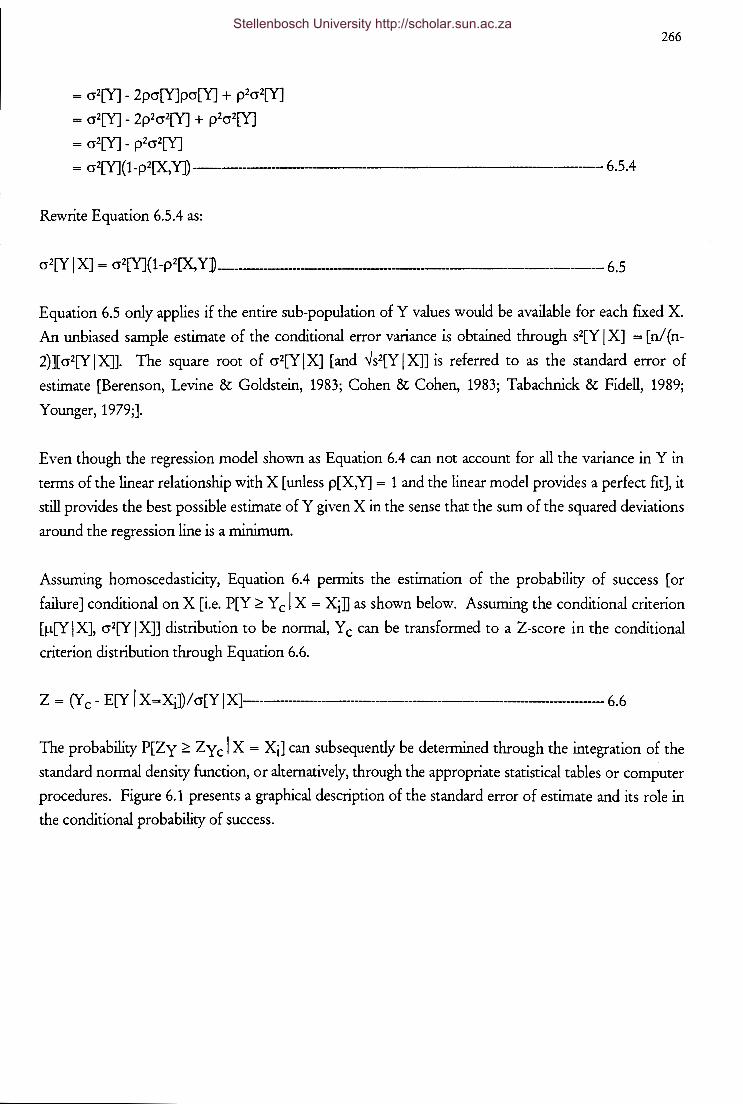
= cr2[Y] - 2pcr[Y]pcr[Y] + p2cr2[Y]
= cr2[Y] _ 2p2cr2[Y] + p2cr2[Y]
= cr2[Y] _ p2cr2[Y]
= cr2[Y](1-p2[X,Y]- -------·------·----- ----6.5.4
Rewrite Equation 6.5.4 as:
cr2[Y I X] = cr2[Y](1-p2[X,Y] ____________ . ___________________________ 6.5
266
Equation 6.5 only applies if the entire sub-population of Y values would be available for each fixed X.
An unbiased sample estimate of the conditional error variance is obtained through s2[Y I X] = [n/(n-
2)][ cr2[Y I X]]. The square root of cr2[Y I X] [and '-'s2[Y I X]] is referred to as the standard error of
estimate [Berenson, Levine & Goldstein, 1983; Cohen & Cohen, 1983; Tabachnick & Fidell, 1989;
Younger, 1979;].
Even though the regression model shown as Equation 6.4 can not account for all the variance in Y in
terms of the linear relationship with X [unless p[X,Y] = 1 and the linear model provides a perfect fit], it
still provides the best possible estimate of Y given X in the sense that the sum of the squared deviations
around the regression line is a minimum.
Assuming homoscedasticity, Equation 6.4 permits the estimation of the probability of success [or
failure] conditional on X [i.e. P[Y ~ Y c I X= Xi] as shown below. Assuming the conditional criterion
[!J.[Y I X], cr2[Y I X]] distribution to be normal, Y c can be transformed to a Z-score in the conditional
criterion distribution through Equation 6.6.
Z = (Y c - E[Y I X= Xi]) I cr[Y I X]-------------------------------------------------------------- 6. 6
The probability P[Zy ~ Zy c I X = Xi] can subsequently be determined through the integration of the
standard normal density function, or alternatively, through the appropriate statistical tables or computer
procedures. Figure 6.1 presents a graphical description of the standard error of estimate and its role in
the conditional probability of success.
Stellenbosch University http://scholar.sun.ac.za
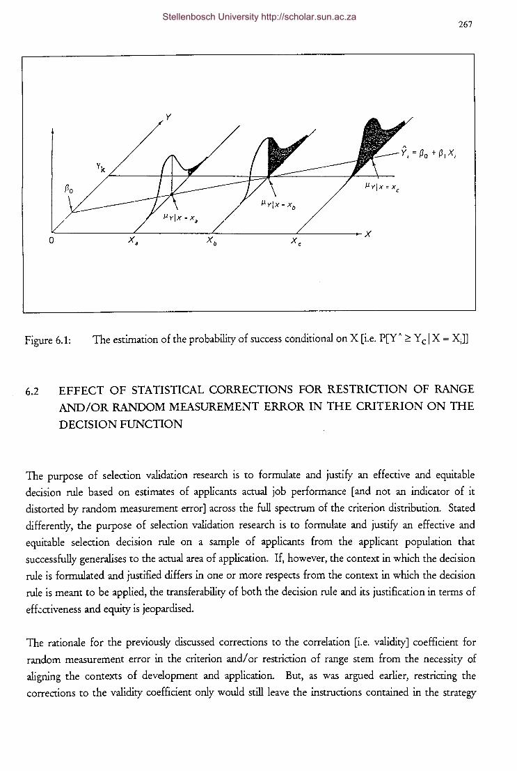
267
Figure 6.1: The estimation of the probability of success conditional on X [i.e. P[Y A ~ Y c I X = XJ]
6.2 EFFECT OF STATISTICAL CORRECTIONS FOR RESTRICTION OF RANGE
AND/OR RANDOM MEASUREMENT ERROR IN THE CRITERION ON THE
DECISION FUNCTION
The purpose of selection validation research is to formulate and justify an effective and equitable
decision rule based on estimates of applicants actual job performance [and not an indicator of it
distorted by random measurement error] across the full spectrum of the criterion distribution. Stated
differently, the purpose of selection validation research is to formulate and justify an effective and
equitable selection decision rule on a sample of applicants from the applicant population that
successfully generalises to the actual area of application. If, however, the context in which the decision
rule is formulated and justified differs in one or more respects from the context in which the decision
rule is meant to be applied, the transferability of both the decision rule and its justification in terms of
effectiveness and equity is jeopardised.
The rationale for the previously discussed corrections to the correlation [i.e. validity] coefficient for
random measurement error in the criterion and/ or restriction of range stem from the necessity of
aligning the contexts of development and application. But, as was argued earlier, restricting the
corrections to the validity coefficient only would still leave the instructions contained in the strategy
Stellenbosch University http://scholar.sun.ac.za
268
matrix unaffected. The decision strategy actually applied for decision making would thus still be the
one derived from a simulated application, which, however, is not fully representative of the actual
application. This naturally should lead to the question whether the aforementioned factors that
produce bias in the validity coefficient obtained from a simulated application in the development
environment also systematically affects the parameters of the decision function [specifically, a, p, E[Y I Xi] & P[Y ~ Y c I X = Xi]. If in fact one or more of these situational characteristics do introduce
bias in one or more of these parameters, the logical further question arises how to correct for the
biasing effect of random measurement error in the criterion and/ or restriction of range comparable to
the various previous corrections to the correlation [i.e. validity] coefficient. Finally, should such
corrections prove to be practical, the following additional questions are raised:
~ would such corrections change decisions on employment applicants?; and if so
~ what would the value of the consequences of the change in decisions be?; and
~ how would the cost of the corrections compare to the value of the changed
decisions affected by the corrections?.
The fundamental a priori position underlying these latter questions is that such corrections would serve
very little, if any, practical purpose if they do not change the actual decisions on applicants for
employment or do so at a cost exceeding the value of the change in decisions.
6.2.1 Effect Of Statistical Corrections For Random Measurement Error On The Decision
Function
6.2.1.1 Effect Of Statistical Corrections For Random Measurement Error In The Criterion On
The Decision Function
The effect of removal of measurement error from the criterion only on the parameters of the simple
linear model is examined in Equation 6.7.
The expected true criterion score, conditional on the observed predictor score can be written as:
E[Ty I Xi] = a 1 + P 1 Xi------------------------------------------------------------------------------------ 6.7 .1
Where;
a1 = E[Ty]- P1E[X]
Stellenbosch University http://scholar.sun.ac.za
= !J[Y]- P1!l[XJ------------------------------------------------------------ 6.7.2
and:
P1 = p[X,Ty](cr[Ty]/cr[X])
= (p[X,Y]/ "Ptt y){ "Ptt y( cr[Y]/ cr[X])}
= p[X,Y]( cr[Y]/ cr[X]) ----------------------------- 6.7 .3
Substituting Equations 6.7.2 and 6.7.3 in Equation 6.7.1:
E[Ty I Xi]= (!l[Y]- P1!l[X]) + Pt Xi
= !l[Y] + p 1 (Xi - !l[X])
= !J[Y] + p[X,Y](cr[Y]/cr[X])(Xi- !J[X])
= E[Y I Xi] --------------------------------------------------------------------------------------------- 6. 7
269
Equation 6.7 indicates that the decision function remains unaffected by the partial correction for
attenuation. Thus neither the Y -axis intercept nor the X -axis slope are affected by the removal of
random measurement error from the criterion. The position of applicants in the strategy matrix,
consequently, will also remain unaffected since E[Ty I X]= E[Y I X]. The decisions on applicants will therefore not change due to the partial correction for attenuation.
Equation 6.8 points to the same conclusion by indicating that E[Ty I X] and E[Y I X], standardised on
the original, fallible criterion distribution, coincide.
Let Z 1 represent the standardised E[Y I X]
Let z2 represent E[Ty I X] standardised on the fallible criterion distribution
Expressing the deviation of the expected observed criterion score conditional on the observed
predictor score from the criterion mean in terms of the standard deviation of the observed criterion
distribution:
Z 1 = (E[Y I X] - !J[Y])/ cr[Y]------------------------------------------------------------------------------------ 6.8.1
Substituting Equation 6.1 in Equation 6.8.1:
z1 = (a+ p[Y I X]X- 1-l[YJ)/cr[YJ-------------------------------------------------------------------------------- 6.8.2
Stellenbosch University http://scholar.sun.ac.za
270
Substituting equation 6.2 in Equation 6.8.2:
Z 1 = (~[Y] - p[Y I X]~[X] + p[Y I X]X - ~[Y]) I cr[Y]
= p[Y I X] (X - ~[X])/ cr[Y]------------------------------------------- ·----- 6.8.3
Substituting Equation 6.3 in Equation 6.8.3:
zl = (p[X,Y]cr[Y](X- ~[X])/(cr[X]cr[Y])
= (p[X,Y](X - ~[X])) I a [X]---------------------------------------------------------- 6. 8. 4
Similarly, expressing the deviation of the expected true criterion score conditional on the observed
predictor score from the criterion mean in terms of the standard deviation of the observed criterion
distribution:
Z 2 = (E[Ty I X] - ~[Y]) I cr[Y]
= ( a[T y I X] - P [T y I X] - ~[[Y]) I cr[Y]---------------------------------------------------------------------- 6. 8. 5
Substituting Equation 6.7 in Equation 6.8.5:
z2 = {~[Y] + p[X,Y](cr[Y]/cr[X])(Xi- ~[X])- ~[Y]}/cr[Y]
= (p[X, Y] (X - ~[X])) I a [X]-------------------------------------------------------------------------------- 6. 8. 6
Therefore:
Z1/Z2 = {(p[X,Y](X- ~[X]))/cr[X]}{cr[X]/(p[X,Y](X- ~[X]))}
= 1 -------------------------------------------------------------------------------------- 6. 8
Therefore:
z1 = z2
The critical criterion cutoff value, Y 0 is defined on a scale unaffected by [systematic and/ or random]
measurement error. Y c thus reflects the minimum actual contribution considered acceptable.
Equation 6. 9 indicates that the removal of random measurement error from the criterion consequently
has the effect of increasing the absolute value of Y c expressed as a Z-score standardised on the
infallible criterion distribution. Y c thus effectively shifts away from the mean as a function of Ptt y
thereby reducing the proportion of the criterion distribution falling above Y c [i.e. the base rate] if Y c > ~[Y] or increasing the base rate if Y c < J..l[Y].
Stellenbosch University http://scholar.sun.ac.za

Let Z 1 represent the standardised criterion cutoff in the original criterion distribution
let z2 represent the standardised criterion cutoff in the disattenuated criterion distribution
The criterion cutoff standardised on the original criterion distribution can be expressed as:
Z 1 = (Y c - 1-1[Y])/ cr[Y] ------------------------------------------------------- 6. 9.1
The criterion cutoff standardised on the true score criterion distribution can be expressed as:
Z 2 = (Y c - 1-1[Y]) I ( cr[Y]--J Ptt y )-------------------------------------------------------------------- 6. 9.2
Therefore:
Z1/Z2 = ((Y c- 1-![Y])/cr[Y])(cr[Y]--Jptty)(Y c- 1-1[Y])
= --JPttY ~ 1-------------------------------------------------------------------------------------------------------------- 6. 9
Therefore:
And;
Therefore:
271
Although the expected criterion performance conditional on X is not affected by the partial correction
for attenuation, the relative position of the expected performance in the criterion distribution does
change as shown by Equation 6.10. Comparing Equations 6.9 and 6.10, however, indicates that the
change in the position of Y c relative to the change in the position of the expected criterion
performance is of the same magnitude and in the same direction. The corrections, therefore, do not
affect the position of the expected performance relative to Y c· The decisions on applicants will
therefore not change due to the partial correction for attenuation.
Stellenbosch University http://scholar.sun.ac.za
272
Let Z1 represent the expected observed score criterion performance conditional on Xi E[Y I Xi]
standardised on the observed score criterion distribution.
Let Z2 represent the expected true score criterion performance conditional on Xi E[Ty I Xi]
standardised on the true score criterion distribution.
According to Equation 6.8.4, the expected observed score criterion performance conditional on Xi
standardised on the observed score criterion distribution can be expressed as:
Z 1 = (E[Y I Xi] - J.L[Y]) I cr[Y]
= (p[X,Y]cr[Y](X- J.L[X]))I(cr[X]cr[Y])
= (p[X, Y] (X - J.L[X])) I cr[X] ------------------------------------------------------------------------------- 6.1 0.1
The expected true score criterion performance conditional on Xi, standardised on the true score
criterion distribution can be expressed as:
z2 = (E[Ty I X]- J.L[Y])Icr[Ty]
= (E[T y I X] - J.L[Y]) I ( cr[Y]..J Ptt y) -------------------------------------------------------------------------- 6.10 .2
Substituting Equation 6.7 in Equation 6.10.2:
Z2 = {J.L[Y] + p[X,Y](cr[Y]Icr[X])(Xi- J.L[X])- J.L[Y]}I(cr[Y] PttY)
= { p[X,Y]()\ - J.L[X])} I ( cr[X]..J Ptt y) ------------------------------------------------------------------------- 6.1 0.3
Therefore:
Z 1 IZ 2 = { (p[X,Y]()\ - J.L[X]) )I cr[X] }{ ( cr[X]..J Ptt y) I (p[X,Y](Xi - J.L[X])}
= ..JPttY
::; 1---------------------------------------------------------------------------------------------- 6.10. 4
Therefore:
The preceding argument, however, applies only if the information way of the strategy matrix is
expressed in terms of expected criterion performance. Should the information way of the strategy
matrix be expressed in terms of the conditional probability of success, attention turns to the standard
error of estimate as the critical factor [assuming Y c to remain unaffected]. Equation 6.11 reflects the
Stellenbosch University http://scholar.sun.ac.za
273
effect of statistically removing random measurement error from the criterion on the standard error of
estrrnate.
According to Equation 6.5:
cr2[Y I X] = cr2[YJ(1 - p2[X,Y])- -------
Therefore:
cr2[Ty I X]= cr2[Ty](1- p2[X,Ty]
= PttYcr2[Y]{1- (P2[X,Y]/ptty)}
= PttYcr2[Y]- PttYcr2[Y](p2[X,Y]/ PttY)
= Ptt ycrz[Y] - cr2[Y]p2[X,Y]
= cr2[YJ(PttY- p2[X,Y])
------------------------- 6.11.1
~ cr2[Y I X] ------------------------------------------------------------------------------------------------------ 6.11
Therefore:
cr[Ty I X] ~ cr[Y I XJ
The effect of statistically removing random measurement error from the criterion is to reduce the
standard error of estimate. The critical question is how this affects the conditional probability of
success. Assuming a constant Y 0 only the reaction of the standard of estimate to the removal of
random measurement error from the criterion needs to be taken into consideration since the
parameters of the decision function [i.e. the expected criterion performance] remain invariant. The
decrease in the standard error brought about by the removal of measurement error from the criterion,
will have the effect of translating the critical criterion cutoff to a more extreme Z-score as shown by
Equation 6.12.
Let Z 1 represent the standardised Y c in the fallible conditional criterion distribution
Let Z 2 represent the standardised Y c in the infallible conditional criterion distribution
The critical criterion cutoff Y c standardised on the fallible conditional criterion distribution can be
expressed as:
Z 1 = (Y c- E[Y I Xi])/ cr[Y I X]--------------------------------------------------------------------------------------- 6.12.1
Stellenbosch University http://scholar.sun.ac.za
274
Substituting Equation 6.5 in Equation 6.12.1:
21 = (Y c - E[Y I Xi])/ { cr[Y]..J(1-p2[X,Y] }----------------------------------6.12.2
The critical criterion cutoff Y c standardised on the infallible conditional criterion distribution can be
expressed as:
22 = (Y c- E[Ty I Xi])/ cr[Ty I X]------------------------------------------ 6.12.3
Substituting Equations 6.7 and 6.11 in Equation 6.12.3:
22 = (Y c- E[Y I Xi])/(cr[Y]..Jptty-p2[X,Y]------------------------------------------------------- 6.12.4
Therefore:
21/22 = { (Y c- E[Y I Xi])/ cr[Y]..J(1-p2[X,Y])}(cr[Y]..JpttY-P2[X,Y])/(Y c- E[Y I Xi])
= (..Jptty-pz[X,Y])/..J(1-p2[X,Y])
:::; 1------------------------------------------------------------------------------------------------------------ 6 .12
Therefore:
The precise effect on P[Ty ~ Y c I X = Xi], moreover, will depend on the position of Xi relative to Xc
= (Y c - a)/p [i.e. P[Y ~ Y c I X = XcJ = 0.50]. For all Xi < Xc, P[Ty ~ Y c I X =Xi] will decrease
relative to P[Y ~ Y c I X = Xi] and for all Xi > Xc, P[Ty ~ Y c I X = Xi] will increase relative to P[Y ~ Y c I X = Xi]. For Xi = Xc, P[Y ~ Y c I X = Xi] will remain unaffected.
Partially correcting the standard error of estimate for the attenuating effect of criterion unreliability will,
however, very unlikely change the selection decisions on applicants when selection is restricted by
quotas. Although the conditional probabilities are altered by the correction, the rank-order of the
applicants in terms of their chances of success remain exactly the same. Consequently, the same top
Nv would still be selected. Partially correcting the standard error of estimate for the attenuating effect
of criterion unreliability will only affect restricted selection if an insufficient number of applicants
initially [i.e. prior to corrections] meet the entry requirement as.
In the case of unrestricted selection, however, partially correcting the standard error for criterion
unreliability could affect the selection decision on applicants by increasing the number of applicants
Stellenbosch University http://scholar.sun.ac.za
275
qualifying for selection [assuming as > 0.50]. Correcting the standard error for criterion unreliability
has the effect of pushing any conditional probability greater than 0.50 but less than as [assuming as > 0.50] towards, and possibly past, as, thus increasing the selection ratio. Correcting the standard error
for criterion unreliability has the effect of pushing the critical predictor cutoff corresponding to the
critical probability as towards the point Xc [as defined above] in the predictor distribution. The
selection ratio is consequendy increased for any as > 0.50 and decreased for any as < 0.50 [although
the chance of such a liberal entry requirement seems unlikely].
6.2.1.2 Effect Of Statistical Corrections For Random Measurement Error In Both The Criterion
And The Predictor On The Decision Function
The effect of removal of measurement error from both the criterion and the predictor on the
parameters of the simple linear model is examined in Equation 6.13.
The linear regression of the true criterion scores on the true predictor scores can be expressed as:
E[Ty I TxJ = a[Ty I TxJ + p[Ty I TxJTx----------------------------------------------------------------- 6.13.1
The intercept parameter in Equation 6.13.1 can be expressed as:
a[Ty I TxJ = E[Ty]- p[Ty I Tx]E[TxJ
= J.t[Y] - p[T y I T xJJ.t[X]----------------------------------------------------------------------------- 6.13. 2
The slope parameter in Equation 6.13.1 can be written as:
p[T y I T xJ = p[T x, T y] ( cr[T y v cr[T x] ---------------------------------------------------------------------- 6.13. 3
Substituting Equations 3.1 and 2.16 in Equation 6.13.3:
p[T y I T xJ = { p[X,Y]/ (" Ptt y" pttX) }{ "Ptt ycr[YJ/ (" PttXcr[X])}
= (p[X,Y)(cr[Y]/cr[X](1/"pttX)
= ( 1 I Pttx) p[Y I X] ---------------------------------------------------------------------------------- 6.13. 4
Therefore:
E[Ty I T Xi] = Jl[Y] + (p[X,Y]/ Ptt:x) ( cr[YJ/ cr[X]) (T Xi - !l[X]
Stellenbosch University http://scholar.sun.ac.za
276
* E[YIXi]
* E[Ty I Xi]------------------------------------ 6.13
Equation 6.13 indicates that the decision function derived from infallible [i.e. perfectly reliable]
predictor and criterion data differs from the decision function derived from fallible criterion and
predictor data. The effect of the removal of random measurement error from both the dependent and
independent variables is to increase the slope parameter P and to decrease the intercept parameter a as
a function of PttX: This implies that the regression equation derived from fallible data and the
regression equation derived from infallible data will intersect at some point Xs. The point of
intersection Xs coincides with the mean of the predictor distributions [i.e. J.L[X] = J.L[Tx]J since
E[Ty I Tx = J.LlfxJJ = J.L[Y] = E[Y I x = J.L[XJJ.
The problem with the fully disattenuated correlation coefficient, and thus also with Equation 6.13, in
the context of validation research lies in the fact that a perfectly reliable predictor will never be
available. Tx can therefore never be obtained directly. The actual effect of substituting the regression
equation derived from fallible data [Equation 6.4] with an equation derived from infallibl~ data
[Equation 6.13] can thus never be assessed since the reaction of individual X-values to the removal of
their random measurement error component can never be ascertained.
Although Tx can never be directly calculated, it can nonetheless be estimated through Equation 6.14,
albeit with some error.
The linear regression of the true predictor scores on the observed predictor scores can be expressed as:
E[Tx I X] = a[Tx I X] + P[Tx I XJXi-------------------------------------------------------------------------- 6.14.1
The intercept parameter in equation 6.14.1 can be expressed as:
a[Tx I X]= J.Llfx]- p[Tx I XJJ.L[X]
= J.L[X] - p[T X I XJJ.L[XJ---------------------------------------------------------------- 6.14 .2
Since J.L[Tx] = J.L[X]
The slope parameter in Equation 6.14.1 can be expressed as:
P[Tx I X]= p[Tx,XJ(cr[TxVcr[X])
= --) PttX--J PttX
= PttX -------------------------------------------------------------------------------------------------- 6.14. 4
Stellenbosch University http://scholar.sun.ac.za
~~ -------------------------------------
Substituting Equations 6.14.2 and 6.14.4 in Equation 6.14.1:
E[Tx I X]= 11[X] -P[Tx I X]!l[X] + P[Tx I XJXi
= ll[X](1- P[Tx I X])+ P[Tx I XJXi
= ll[X](1 - Ptt:x) + PttX Xi----------------------------------------- 6.14
277
Substituting Equation 6.14 into Equation 6.13 results in Equation 6.15 returning the expected actual
criterion performance conditional on the expected true predictor score, conditional on the observed
predictor score. Obtaining an expression for E[Ty I E[fx I X], however, requires more than simply
exchanging Tx in Equation 6.13 with Equation 6.14. To do so would result in an inaccurate argument
although it would still have led to the same eventual conclusion that E[Ty I E[Tx I X]]= E[Y I Xi] =
E[Ty I Xi]. To obtain an appropriate expression for E[Ty I E[fx I X] requires, in addition, that
p[Ty,Tx] and cr[Tx] be replaced by p[Ty,E[Tx I X]] and cr[E[Tx I X] respectively.
The regression of the true criterion scores on the expected true predictor scores conditional on the
observed predictor scores, can be expressed as:
E[Ty I E[Tx I X]]= a[Ty I E[Tx I X]]+ p[Ty I E[Tx I X]E[Tx I X]------------------------------- 6.15.1
The intercept parameter in Equation 6.15.1 can be expressed as:
a[Ty I E[Tx I X]]= ll[Ty]- p[Ty I E[Tx I XJJ!l[E[Tx I X]
= 11[Y]- p[Ty I E[Tx I XTI!l[XJ---------------------------------------------------------- 6.15.2
The slope parameter in Equation 6.15.1 can be expressed as:
p[Ty I E[Tx I X]]= p[Ty,E[Tx I X]](cr[TyYcr[E[Tx I XJD
= p[T y,X]{ ( cr[Y]'-' Ptt y)/ ( cr[X]ptt:x)}
= (p[X,YY'-'pttY)({cr[Y]'-'PnY)/(cr[X]pttX)}
= (p[X, Y]cr[Y]) I ( cr[X]pttX)
= (11 PtOO p[Y I X]-------------------------------------- 6.15.3
Since, p[Ty,E[Tx I X]] = p[Ty ,X] since Tx is a linear function of X
and
Stellenbosch University http://scholar.sun.ac.za

Substituting Equation 6.15.2 in Equation 6.15.1:
E[Ty I E[Tx I X]] = a[Ty I E[Tx I X] + p[Ty I E[Tx I X]E[Tx I X]
= )l[Y] - p[Ty I E[Tx I X])l[XJ + p[Ty I E[fx I X]E[Tx I XJ
= )l[Y] + p[fy I E[Tx I X](E[Tx I XJ- )l[X]-------------------------- 6.15.4
Substituting Equation 6.15.3 in Equation 6.15.4:
E[Ty I E[Tx I XJJ = )l[Y] + p[Ty I E[Tx I X](E[Tx I XJ- )l[X]
= )l[Y] + (1/pttX)p[YIXJ(E[Tx I XJ- )l[X]
= )l[Y] + (1/ pttX) {p[X,Y](cr[Y]/ cr[X]} (E[Tx I X]- )l[X]------------------ 6.15
278
Equation 6.15, similar to Equation 6.13, differs from the fallible regression equation and the partially
attenuated regression equation [Equation 6.4] in terms of both intercept and slope. The regression of
Ty on E[Tx I X] has a steeper slope and a lower intercept than the regression of Yon X. The increase
in slope is a function of 1/ PttXi thus the less reliable the predictor measurements the greater the
increase in the slope and the corresponding decrease in intercept. The regression of Ty on E[Ty I X],
furthermore, corresponds to the regression of Ty on Tx in terms of intercept and slope.
Since it is possible to obtain the regression of Ty on Tx from the regression of Ty on E[Tx I Xl the
temptation exists to conclude that the possibility presents itself to obtain a closer estimation of
E[Ty I TxJ than is possible through E[Ty I X]. One should, however, be careful in concluding that the
change in the decision function implies a concomitant change in the expected criterion performance
associated with the various applicants. In assessing the effect of fully disattenuating the parameters of
the decision function, the regression of E[Tx I X] and E[Ty I Y] towards their respective means must
be kept in mind. The change in the predictor information entering the regression equation and the
change in the regression parameters must consequently be considered simultaneously to assess the
change in the expected criterion performance attributable to Equation 6.15.
Let Z 1 represent the expected criterion performance obtained from the fallible regression equation
[Equation 6.4], standardised on the fallible criterion distribution.
Let Z2 represent the expected criterion performance obtained from Equation 6.15 standardised on the
fallible criterion distribution.
The expected observed criterion performance, conditional on Xi, standardised on the fallible criterion
distribution can be expressed as:
Stellenbosch University http://scholar.sun.ac.za
Z 1 = (E[Y I Xi] - J.t[Y]) I a[Y] ------------------------------------------------------------ 6.16.1
Substitute Equations 6.1, 6.2 and 6.3 in Equation 6.16.1:
Z1 =(a+ P[YIX]Xi -J.t[Y])Icr[Y]
= (J.t[Y] - P[Y I X]J.t[X] + P[Y I X]Xi - J.t[Y])I cr[Y]
= P[Y I X] (Xi- J.t[X])I cr[Y]
= (p[X,Y]cr[Y])I { cr[X](Xi - Jl[X])I cr[Y]}
= (p[X,Y]I cr[X]) (Xi - J.t[X]) ---------------------------------------------------------- 6.16.2
279
The expected true score criterion performance obtained from Equation 6.15 standardised on the fallible
criterion distribution can be expressed as:
Z 2 = (E[Ty I E[T X I X]] - J.t[Y]) I cr[Y}-------------------------------------------------------------------------- 6.16.3
Substituting Equations 6.15.1 and 6.15.2 in Equation 6.16.3
Z2= (a+ p[Ty I E[Tx I X]]E[Tx I Xi]-J.t[Y])Icr[Y]
= (J.t[Y]- p[Ty I E[Tx I XJ]J.t[X] + p[Ty]E[Tx I Xi] -J.t[Y])Icr[Y]
= p[Ty I E[Tx I X]](E[Tx I Xi]- J.![X])Icr[Y]-------------------------------------------------------------- 6.16.4
Substituting Equation 6.15.3 in Equation 6.16.4:
Z2= {(p[X,Y]cr[Y])I(cr[X]pttX)}(E[Tx I Xi]- J.![X])Icr[Y]
= { (p[X, Y]) (E[T x I Xi] - J.![X]) } I ( cr[X]pux) --------------------------------------------------------·-- 6 .16. 5
Substituting Equation 6.14 in Equation 6.16.5:
z2 = {(p[X,Y])((J. + PttXXD- j.![X])}I(cr[XJPtW
= { (p[X,Y]) (J.![X] - J.![XJPttX + PttX Xi - J.![X]) }/ ( cr[XJPtW
= {(p[X,Y])(J.![X]pttX + PttXXD}I(cr[X]pux)
= {(p[X,Y])(PuXCXi- J.![X]))}I(cr[X]pttX)
= { (p[X,YJ) CXi - J.![XJ)} I ( cr[XJ) ---------------------------------------------------------------------------- 6.16.6
Therefore:
Z 1 /Z 2 = (p[X,Y]/ cr[X]) (Xi - J.![X]) ( cr[X])/ { p[X,Y](Xi - J.![X])}
= 1 --------------------------------------------------------------------------------------------------------------- 6.16
Stellenbosch University http://scholar.sun.ac.za
280
Therefore:
Equation 6.16 indicates that the corrections have no effect on the expected criterion performance. The
expected Ty performance derived through Equation 6.15 equals the expected criterion performance
derived through the uncorrected regression of Yon X or partially corrected regression of Ty on X.
The removal of random measurement error from both the dependent and independent variables will
consequently have no affect on the applicants selected irrespective of whether selection is restricted by
quotas or not and strict top down selection applies ..
The issue can, however, also be approached from the perspective of the predictor. Assume a critical
predictor cutoff Xc = (Y c-a[Y I X])/~[Y I X], so that E[Y I X =XJ = Y c and assume a critical expected
true score Xcc = (Yc-a[Y I E[Tx I X]J)/~[Ty I E[Tx I X], so that E[T I E[Tx I X]=XJ = Yc.
Equation 6.17 indicates that the ratio of the standardised Xc [Z1] to Xcc standardised on the original
predictor distribution [Z2J always will equal or exceed unity, which implies that Xcc will either coincide
with Xc or occupy a less extreme position than Xc in the original predictor distribution.
The critical predictor cutoff derived from the equation describing the regression of the fallible criterion
scores on the fallible predictor score [Equation 6.4], can be expressed as:
Xc = (Y c- a[Y I X])/~[Y I X]
= (Y c - (~[Y] - ~[Y I X]~[XJ))/~[Y I X]
= Y ci~[Y I X]- ~[Y]/~[Y I X] + ~[X] = (1/~[Y I X])(Y c- ~[Y]) + ~[X] = ( cr[X]/ (p[X, Y]cr[Y])) (Y c - ~[Y]) + ~[X]---------------------------------------------------------------- 6.17 .1
Similarly from Equation 6.15 follows that the critical predictor cutoff derived from the equation
describing the regression of the true criterion scores on the estimated true predictor scores, can be
expressed as:
Xcc = 1/~[Ty I E[Tx I X]J(Yc- ~[Y]) +~[X] = ( cr[X]pttX/ (p[X,Y]cr[Y])) (Y c - ~[Y]) + ~[X]--------------------------------------------------------- 6.17 .2
Let Z 1 represent the standardised Xc
Stellenbosch University http://scholar.sun.ac.za
Let Z 2 represent Xcc standardised in terms of the fallible predictor distribution
Consequently:
Z/Zz = ((Xc- ~[X])/ cr[X])/ { (Xcc- ~[X])/ cr[XJ}
= ((Xc- ~[X])/cr[X](cr[X]/(Xcc- ~[X]))
= ((Xc- ~[X])I(Xcc- ~[X]))------------------------------------------ 6.17.3
Substituting Equations 6.17.1 and 6.17.2 in Equation 6.17.3:
Z 1/Z2 = { (cr[X]/ (p[X,Y]cr[Y]) (Y c-~[Y])+
~[X]-~[XJ} I { ( cr[X]Pnxl (p[X,Y]cr[Y])) (Y c-~[Y])+ ~[X]-~[X]}
= {cr[X]/(p[X,Y]cr[Y])}(Yc- ~[Y])(p[X,Y]cr[Y])(1/cr[XJpttX)(1/(Yc- ~[Y])
= liPttX 2:: 1--------------------------------------------------------------------------------------------------------------------- 6.17
Therefore:
and:
281
How this shift in the critical predictor affects the selection ratio will, however, depend on the direction
and magnitude of the shift in the predictor informa~ion produced by Equation 6.15
Equation 6.18 [see also Equation 6.14] indicates the effect of the removal of random error variance
from the predictor and the estimation of the true predictor score on the relative position of applicants
in the original predictor distribution. Since Z1/Z2 2:: 1 it implies that the estimated true score returned
by Equation 6.14 falls numerically closer to the mean of the predictor distribution than the
unattenuated, observed score.
Let Z1 represent the standardised observed predictor score.
Let Z2 represent the estimated true predictor score standardised on the original predictor distribution.
An observed predictor score, standardised on the observed predictor distribution can be expressed as:
Stellenbosch University http://scholar.sun.ac.za
282
2 1 = (Xi - J.t[X]) I cr[X] -------------------------------------------------------------- 6.18.1
A true predictor score, estimated from the observed predictor score, standardised on the observed
predictor distribution can be expressed as:
22 = (E[Tx I X]- ~-tDCJ)Icr[X]----------------------------------------- 6.18.2
Substituting Equation 6.14 in Equation 6.18.2:
22 = (J.t[X](1- pttX) + PttXXi- J.t[X])Icr[X]
= (J.t[X] - J.t[X]pttX + PttX Xi - J.t[X])I cr[X]
= PttX (Xi - J.t[X]) I cr[X]--------------------------------------------------------------------------------- 6.18.13
Therefore:
21122 = (Xi- J.t[X])(11cr[X])(cr[X])(11 PttX(Xi- J.t[X])
= liPttX
~ 1---------------------------------------------------------------------------------------------------------- 6.18
Therefore:
and:
It thus follows that the magnitude of the Xi ~ E[Tx I Xi] movement towards the predictor mean
equals the magnitude of the Xc ~ Xcc movement towards the mean. Consequently the number of
applicants satisfying the condition E[Tx I Xi]~ Xcc will equal the number of applicants satisfying the
condition Xi ~ Xc.
Selection decisions can be based either on E[Y I X] or P[Y> Y c I X]. The latter is dependent on the
former as well as on the conditional criterion variance [i.e., the standard error of estimate]. Equation
6.19 reflects the effect of statistically removing random measurement error from both the criterion and
the predictor via Equation 6.15 on the standard error of estimate.
According to Equation 6.5:
Stellenbosch University http://scholar.sun.ac.za
cr2[Y I X]= cr2[Y](1- p2[X,Y])-------------------------------------------------------- 6.19.1
Therefore:
cr2[Ty I E[Tx I Xi]] = cr2[Ty ](1 - p2[Ty,E[Tx I Xi}
= PttYcr2[YJ{1- (p2[X,Y]/ptty)}
Thus:
= PttYcr2[Y]- PttYcr2[Y](p2[X,Y]/pttY)
= PttYcr2[YJ- cr2[YJ(p2[X,Y]
= cr2[Y]{PttY- P2[X,Y]}
= cr2[Ty I X]::; cr2[Y I X]----------------------------------------------------------------- 6.19.2
cr[Ty I E[Tx I Xi]] = cr[Ty I X]::; cr[Y I X]-------------------------------------------------------------------- 6.19
283
The effect of statistically removing random measurement error from the both the criterion and
predictor essentially duplicates the effect of partially correcting the standard error of estimate for
criterion unreliability only. The results reported earlier thus also apply to Equation 6.19. Such would
not have been the case had it not been for the fact that the parameters of the decision function react to
the removal of random measurement error from both the criterion and the predictor in a way that
leaves the expected criterion performance unaltered. An analysis of the effect of fully disattenuating
the standard error of estimate on the conditional probability of success and eventually selection
decision-making would otherwise have had to simultaneously consider the reduction in the standard
error of estimate and the change in the parameters of the decision function [i.e. E[Y I Xi] relative to Y cJ.
Equation 20, assuming a constant critical criterion cut-off defined on the true criterion scale, indicates
that the removal of random error variance from both the criterion and the predictor has the effect of
shifting the relative position of Y c outwards in the conditional criterion distribution. Equation 6.20
assumes that Y c > f.![Y].
Let Z 1 represent the standardised Y c in the uncorrected conditional criterion distribution
Let Z2 represent the standardised Y c in the corrected conditional criterion distribution
Based on Equation 6.5, the standardised Y c in the uncorrected conditional criterion distribution can be
expressed as:
Z1 = (Y c E[Y I Xi])/cr[Y I X]
= (Y c - E[Y I Xi]) I cr[Y]~ { ( 1 - P2[X,Y])} ------------------------------------------------------------- 6.20.1
Stellenbosch University http://scholar.sun.ac.za
284
Based on Equation 6.11, the standardised Y c in the corrected conditional criterion distribution in turn
can be expressed as:
z2 = (Y c- E[Ty I E[Tx I XiJD/ { cr[Y]'-'(PttY- p2[X,Y])}--------------------------- 6.20.2
Consequently:
Z1/Z2 = {(Y c-E[Y I Xi])/(cr[Y]'-'(1-p2[X,Y])) }{ cr[Y]'-'(PttY-P2[X,Y])/(Y c-E[Ty I E[Tx I Xi]])}
= { (Y c-E[Y I Xi])1'-'(1-p2[X,Y])}{ '-'(PttY-P2[X,Y])/(Y c-E[Y I Xi])}
= H(PttY-P2[X,Y]) }1'-'(1-p2[X,Y])
s 1------------------------------------------------------------------------------------------- 6.20
And consequently that the standardised Y c in the uncorrected conditional criterion distribution
occupies a less extreme position in the fallible criterion distribution than it does in the corrected
conditional criterion distribution:
The precise effect of statistically removing random measurement error from both the predictor and the
criterion on P[Ty ~ Y c I E[Tx IX]] will depend on the position of Txi relative to Xcc [or Xi relative to
XcJ. The fully disattenuated conditional probability of success will increase relative to P[Y ~ Y c I X] for
all applicants with expected criterion performances greater than the critical criterion cut-off while it
would decrease relative to P[T ~ Y c I X] for all applicants with E[Y I X] < Y c· P[T y ~ Y c I E[f X I X]
will consequently provide a closer approximation of P[Ty ~ Y c I Tx] than the attenuated conditional
probability of success.
The fully disattenuated standard error of measurement applicable to Equation 6.13 could likewise be
determined but would, like Equation 6.13, have relatively little practical utility since E[Ty I Tx]c<n not
be estimated and hence P[Ty ~ Y c I Tx] will remain an unattainable quantity.
The conditional true score criterion variance applicable to Equation 6.13 can be expressed as Equation
6.21:
cr2[Ty I TxJ = cr2[Ty](1- p2[Ty,Tx)
= Ptt ycr2[Y] { 1 - p2[X,Y]/ (Ptt ypttX)}
= Ptt y cr2[YJ - cr2[Y]p2[X,Y]/ PttX
Stellenbosch University http://scholar.sun.ac.za
285
= cr2[Y]( Ptt Y - P2[X,Y]/ Pttx) ~ cr2[Ty I E[Tx IXJ] = cr2[Ty I X]~ cr2[Y I X]--------------~----------- 6.21
Thus:
cr[Ty I TxJ ~ cr[Ty I E[Tx I Xi]= cr[Ty I X]~ cr[Y I X]
Basing selection decision-making on the expected true cntenon performance estimated through
Equation 6.14 from the regression of Ty on the expected true predictor performance conditional on
the observed predictor score instead of E[Y I X] estimated from the regression of Y on X, does not
affect the number of applicants qualifying for restricted or unrestricted selection.
Correcting the parameters of the regression equation and the standard error of estimate for criterion
and predictor unreliability will, however, in the case of on a positive criterion, increase the conditional
probability of success for all applicants with E[Y] > Y c·
The removal of random measurement error from both the criterion and the predictor will unlikely
affect the selection decision if a selection quota is in force and the principle of strict top down selection
applies since the . corrected conditional probabilities are linearly related to the original, uncorrected
probabilities. The same top Nv applicants will, consequently, still be selected. The correction could
only affect restricted selection decision-making if the number of applicants initially fulfilling the
selection requirement[ as] based on the uncorrected conditional probabilities are less than the number
required.
In the case of selection unrestricted by quotas, however, the selection decision will be affected. The
preceding results imply that a number of applicants who initially did not succeed in qualifying could in
fact now satisfy the entry requirement after the corrections [assuming as ~ 0.50]. The selection ratio
[i.e. SR = N /NJ will consequently increase.
Stellenbosch University http://scholar.sun.ac.za
286
6.2.2 Effect Of Statistical Corrections For Restriction Of Range On The Decision Function
6.2.2.1 Case 1 [Case B] Restriction OfRange
Case 1 [Case B] restriction of range refers to the situation when both restricted and unrestricted
variances are known only for the variable on which selection occurs indirectly/incidentally [Gulliksen,
1950].
The focus of interest in validation research is the regression of Y on X. For the current argument the
variable on which selection occurs plays an important role.
If selection occurs directly on the predictor X, but the restricted and unrestricted variances are known
only for the criterion Y, then by assumption neither the regression of Y on X nor the criterion variance
conditional on X will be affected. Thus, by assumption Equations 6.22 and 6.23 apply. The same
notation convention as before is used.
0[Y I X]= p[X,Y](cr[Y]/cr[X])
= p[x,y](cr[y]/q[x]
= 0[y I X]-------------------------------------------------------------------------------------------------------- 6.22
cr2[Y I X] = cr2[Y](1 - p2[X,Y])
= cr2[y](1 - p2[x,y]
= 0[y I X]--------------------------------------------------------------------------------------------------- 6.23
Since Equation 6.22 reflects the assumption that fl(Y I Xi] is not altered by explicit selection on X,
Equation 6.24 also applies.
a[Y I X] = fl[Y] - 0[Y I X]f.l[X]
= f.l(y]- 0[y I X]f.l[X]
= a[y I x] ---------------------------------------------------------------------------------------------- 6.2 4
Although the magnitude of the correlation is influenced by Case 1 [Case B] selection on X, and
although the standard errors of the regression coefficients will increase due to this type of Case 1 [Case
B] selection, the relevant decision function [and therefore also the contents of the strategy matrix] will
not be affected by Case 1 [Case B] selection on X. Corrections to the parameters of the decision
Stellenbosch University http://scholar.sun.ac.za
- --------------------------------------
287
function to compensate for this type of Case 1 [Case B] restriction of range are consequently not
required.
If, in contrast, selection occurs directly on the criterion Y, but the restricted and unrestricted variances
are known only for the predictor X, then by assumption neither the regression of X on Y nor the
predictor variance conditional on Y will be affected. Thus, by assumption the equivalent of Equations
6.22- 6.24 would still apply. In a selection context, however, the interest is not in the regression of X
on Y but rather in the regression ofY on X. The question consequently arises whether Case 1 [Case B]
selection on Y affects the regression of Y on X, Cl!ld if so, how. Intuitively one would expect that
explicit selection on Y should affect the regression of Y on X. Graphical scattergram analysis suggest
that the effect of explicit selection on Y on the regression of Y on X should be a flattening of the
regression slope [i.e. p[y I x] < p[Y I X]] and a concomitant increase in the intercept [i.e. a[y I x] > a[Y I X]]. Equations 6.25 and 6.26 provide analytical confirmation of these inferences by demonstrating
that corrections of the parameters of the decision function for the effect of Case 1 [Case B] selection
on Y produce an increase in the slope parameter and a decrease in the intercept.
Since by assumption the regression of X on Y is not affected by Case 1 [Case B] selection on Y:
p[X I Y] = p[ X I y 1-------------------------------------------------------------------------------------------- 6.25 .1
Substituting Equation 6.3 in Equation 6.25.1:
p[X,Y] ( cr[X]I cr[Y]) = p[ x, y ]( cr[ x ]I cr[y ]) ------------------------------------------------------------------ 6.25. 2
Multiplying Equation 6.25.2 with 11 p[X,Y]:
cr[X]I cr[Y] = (p[ x,y ]I p[X, Y] ( cr[ x ]I cr[y ]) --------------------------------------------------------------------- 6. 25. 3
Multiplying Equation 6.25.3 with 11 cr[X]:
1 I cr[Y] = (p[ x,y ]I p[X,Y]) ( cr[ x ]I cr[y ]cr[X]}--------------------------------------------------------- 6.25 .4
Inverting Equation 6.25.4:
cr[Y] = (p[X, Y]cr[X]cr[y ]) I (p[ x,y ]cr[ x ]) --------------------------------------------------------- 6.25. 5
Substituting Equation 6.3 in Equation 6.25.5:
Stellenbosch University http://scholar.sun.ac.za
~[Y I X]= p[X,Y](cr[YJ/cr[XJ)
= p[X,Y](((p[X,Y]cr[X]cr[y]/(p[x,y]cr[x]))/cr[X])
= (p2[X,Y]cr[y ])/ (p[x,y ]cr[ x ]}------------------------------------------ 6.25.6
However, according to Equation 3.3.5:
p2[X,Y] = 1- (1- p2[x,y])(cr2[x]/cr2[X])
= { 1 - ( cr2[ x ]/ cr2[XJ) + p2[ x,y ]( cr2[ x ]/ cr2[X])}--------------------------------------- 6.25 .7
Substituting Equation 6.25.7 in Equation 6.25.6:
~[Y I X] = { 1 - ( cr2[ x ]/ cr2[X]) + p2[ x,y ]( cr2[ x ]/ cr2[X]) }{ cr[y ]/ (p[ x,y ]cr[ x]}
= cr[y]/(p[x,y]cr[x])- cr[x]cr[y]/(cr2[X]p[x,y] + (p[x,y]cr[x]cr[y]/cr2[XJ
= cr[y ]/ (p[ x,y ]cr[ x ]) - ( cr[ x ]cr[y ]/ (p[ x,y ]cr2[X]){ 1 - p2[ x,y]}------------------------------------ 6.25.8
Therefore:
~[Y I X]/~[y I x]
= {cr[y]/(p[x,y]cr[x])- (cr[x]cr[y])/(p[x,y]cr2[X]{1- p2[x,y]} }/ {p[x,y](cr[y]/cr[x])}
= {cr[y]/(p[x,y]cr[x])- (cr[x]cr[y])/(p[x,y]cr2[X]){1- p2[x,y]} }{cr[x]/p[x,y](cr[y]}
= ( 1 I p2[ x,y ]) - ( cr2[ x ]I p2[ x,y ]cr2[X]) ( 1-p[ x,y]
= ( 11 p2[ x,y ]) - (K 2 I p2[ x,y ]) ( 1-p[ x,y ])---------------------------------------------------------------------------- 6.25. 9
Therefore:
~[Y I X]= ~[y I x]{ (1/ p2[x,y]- (K21 p2[x,y](1-p[x,y])} --------------------------------------6.25
According to Equation 6.24:
a[X I Y] = a[x I y]
Substituting Equation 6.2 in Equation 6.24:
~[X]- ~[X I Y]~[Y] = ~[x]- ~[xI y]~[y}--------------------------------------------------------------- 6.26.1
288
Stellenbosch University http://scholar.sun.ac.za
Therefore:
p[X I Y]~[Y] = ~[X]- ~[x] + p[x I y]~[y]-------------------------------------------------------- 6.26.2
Therefore, since by assumption, p[X I Y] = P[x I y]:
M[Y] = p-1[X I Y](~[X]- ~[x] + P[x I y]~[y]) = p-1[x I y](~[X]- ~[x] + p[x I y]~[y]) = p -1 [X I y] (~[X] - ~[X]) + ~[y ]------------------------------------------------------------------------ 6.2 6. 3
Substituting Equation 6.3 in Equation 6.26.3:
~[Y] = (p[ x,y ]cr[ x ]/ cr[y ])-1 (~[X] - ~[x ]) + ~[y }------------------------------------------------------------- 6.26.4
Substituting Equation 6.26.4 in Equation 6.2:
a[Y I X] = ~[Y] - p[Y I X]~[X] = (p[x,y]cr[x]/cr[y]-1(~[X]- ~[x]) + ~[y]- p[Y I X]~[XJ-------------------------------------- 6.26
With p[Y I X] estimated by Equation 6.25
289
The expression for the regression of Y on X, corrected for Case 1 [Case B] selection on Y, is shown as
Equation 6.27.
E[Y I X] = a[Y I X] + p[Y I XJXi ---------------------------------------------------------------------------------- 6.27 .1
Substituting Equations 6.25 and 6.26 into Equation 6.27.1:
E[Y IX]= (p[x,y]cr[x]/cr[y]-1(~[X]- ~[x]) + ~[y]- p[Y IXJ~[X] + P[Y IXJXi
= (p[x,y]cr[x]/cr[y]-1(~[X]- ~[x]) + ~[y] + p[Y IXJ{Xi- ~[X]}
= (p[ x,y ]cr[ x ]/ cr[y] -1 (~[X] - ~[ x ]) + ~[y] + { cr[y ]/ (p[ x ,y ]cr[ x ]) -
( cr[x ]cr[y ]) I (p[ x,y ]cr2[X]) ( 1 - p2[x,y]} {Xi - ~[X]}----------------------------------------- 6.27
The change in the regression parameters implies that the regression equation derived from the selected
applicant group and the regression equation that would have been obtained from the unrestricted
applicant group will intersect at some point Xs on the X-axis. Consequently, for all Xi < Xs E[y I Xi]
will overestimate E[Y I Xi] while for all Xi > Xs E[y I Xi] v.ill underestimate E[Y I XiJ. Correcting the
parameters of the decision function for Case 1 [Case B] selection on Y, consequently will have the
Stellenbosch University http://scholar.sun.ac.za
290
effect of elevating the expected criterion performance for all Xi > Xs, while depressing it for all Xi <
Xs.
The correction of the decision function for Case 1 [Case B] selection on Y will not affect the applicants
selected if selection is restricted by quotas and strict top down selection applies. Although E[Y I Xi] ::f:.
E[y I Xi], if E[y I Xi] > E[y I Xj] then E[Y I Xi] > E[Y I Xj]. The same Nv applicants would therefore still be
selected.
In the case of selection unrestricted by quotas, however, the use of the corrected decision function will
affect the selection decision-making. The nature of the effect will depend on the position of Xc
[derived from Y c via the decision function calculated on the selected applicant group] relative to Xs . If Xs < Xc the number of applicants satisfying the entry requirement [i.e. E[Y I Xi] > Y cJ will increase. If Xs > Xc [unlikely since it would imply a very low Y c on a positive criterion], the number of applicants
qualifying for selection will decrease.
Case 1 [Case B] selection on X does not affect the standard error of estimate cr[Y I X] [Equation 6.23].
Case 1 [Case B] selection on Y, however, does affect the standard error of estimate cr[Y I X]. Equation
6.28 provides a correction to the standard error of estimate cr[y lx] for Case 1 [Case B] selection on Y.
Since by assumption the regression of X on Y is not affected by Case 1 [Case B] selection on Y:
p[ X I y] = p[X I Y]----------------------------------------------------------------------------------------------------------- 6.28.1
Substituting Equation 6.3 into Equation 6.28.1:
p[ x,y ]( cr[ x ]/ cr[y ]) = p[X,Y] ( cr[X]I cr[Y]) ------------------------------------------------------------------------ 6.28 .2
Multiplying Equation 6.28.2 with cr[Y]cr[y]l p[x,y]cr[x]:
cr[Y] = (p[X, Y]cr[X]cr[y ]) I (p[x,y ]cr[ x] ---------------------------------------------------------------------- 6. 28.3
Substituting Equation 6.28.3 into Equation 6.5:
cr2[Y IX]= cr2[Y](1- p2[X,Y]
=_ { (p2[X, Y]cr2[X]cr2[y] I (p2[ x,y ]cr2[ x ]) }( 1 - p2[X,Y]) --------------------------------------- 6. 28.4
Multiplying the terms in Equation 6.28.4:
Stellenbosch University http://scholar.sun.ac.za
cr2[Y I X] = { (p2[X,Y]cr2[X]cr2[y])/(p2[x,y]cr2[x])} -
{ (p 4[X,Y]cr2[X]cr2[y] I (p2[ x,y ]cr2[ x ]) }---------------------------------------------------- 6.28. 5
Rewrite Equation 6.28.5 with K = cr[x]/cr[X]:
cr2[YIXJ = {(p2[X,Y]cr2[y]/(p2[x,y]K2)}- {(p4[X,Y]cr2[y])/(p2[x,y]K2)}
= cr[y] { p2[X, Y]/ (p2[ x,y ]K 2) - p 4[X,Y]/ (p2[ x,y ]K 2)}
= cr[y]{(p2[X,Y]- plX,Y]/(p2[x,y]K2)}
= cr[y ]{ p2[X,Y] ( 1 - p '[X,Y] I (p2[ x,y ]K 2) } ----------------------------------------------------- 6. 28.6
However, the validity coefficient for the unrestricted applicant group is given by Equation 3.3:
p[X,Y] = v'{1- (1- p2[x,y])(cr2[x]/cr2[X])}
= v'{1- K2(1- p2[x,y]}
Squaring Equation 3.3 and substituting in Equation 6.28.6:
cr2[YIXJ = cr[y]{{1- K2(1- p2[x,y]} (1- {1- K2(1- p2[x,y])})/(p2[x,y]K2)}
= cr[y]{{1- K2(1- p2[x,y]} (K2(1- p2[x,y])/(p2[x,y]K2)}
= cr[y]{(K2(1-p2[x,y])- (K4(1-p2[x,y]2)/(p2[x,y]K2)}
= cr[y]{(1-p2[x,y])- (K2(1-p2[x,y]2)/p2[x,y]}
= cr[y ]{ { (1-p2[x,y ]) }{ 1 - (K2(1-p2[x,y ] 2)/ p2[x,y]} }---------------------------------------------- 6.28
~ cr2[ylx]
291
Analysis of Equation 6.28 indicates that Case 1 [Case B] selection on Y produces an decrease in the
standard error of estimate [i.e. cr[ylxJ < cr[YIXJ]. Correcting cr[y lxJ for Case 1 [Case B] selection on Y
via Equation 6.28 thus returns a corrected value cr[Y I X] greater than the obtained standard error of
estimate. The difference between the corrected and uncorrected standard errors of estimate seems to
be negatively related to the observed correlation p[x,y ].
An analysis of the effect of corrections for Case 1 [Case B] selection on Y, on selection decision making
based on the conditional probability of success, should focus on the relative position of Y c in the
conditional criterion distribution. Since the critical criterion cutoff value, Y 0 is defined on a scale
unaffected by [systematic and/ or random] measurement error, the relative position of Y c in the
conditional criterion distribution depends on the reaction of both the expected criterion performance
and the standard error of estimate to corrections for Case 1 [Case B] selection on Y. A factor
complicating the issue, however, is the fact that the effect of the change in expected criterion
performance on the conditional probability tends to oppose the effect of the change in the standard
Stellenbosch University http://scholar.sun.ac.za
292
error of estimate. The change in the expected criterion performance exerts an upward pressure on the
conditional probability for all Xi > Xs and a downward pressure for all Xi < Xs· The change in the
standard error of estimate, in contrast, produces the opposite effect. The reaction of the conditional
probability of success to the aforementioned corrections for Case 1 [Case B] selection on Y,
consequently, dep~nds on the which one of the two processes dominate. However, no single answer to
this question exists. Since the magnitude of the change in the expected criterion performance depends
on Xi, but the change in the standard error of estimate is constant over all values of Xi, the question on
which one of the processes would dominate would also depend on Xi.
Logic would suggest two points on the X-axis EXhi & X10 ], positioned such on both sides of Xs, that
Z[Yci E[ylx=Xhi]] = Z[Yci E[YIX=XhiJJ and Z[Yci E[yix=Xl0 ]] = Z[Yci E[YIX=Xl0 ]]. The
conditional probability of success associated with applicants falling on Xhi or Xlo wa.Ud therefore not
be affected by the preceding corrections for Case 1 [Case B] selection on Y. Howe~er, for all Xi > Xru, and all Xi < X10 , the effect of the change in expected criterion performance would dominate.
Consequently the conditional probability of success associated with those applicants falling above Xhi
will increase [assuming Y c > !l[Y]], while the conditional probability of success associated with those
applicants falling below Xlo will decrease. Furthermore, for those applicants located between these two
cutoff points [i.e. Xlo < Xi < Xhi], the effect of the change in the standard error of estimate should
dominate and consequently the conditional probability should increase.
The application of Equations 6.27 and 6.28 will [probably] not affect selection decision-making based
on the conditional probability of success, if selection quotas restrict such selection.
The application of Equations 6.27 and 6.28 will, however, affect unrestricted selection decision-making
based on the conditional probability of success. The selection ratio should increase since the critical
acceptance probability as is constant while the conditional probability of success associated with those
applicants falling above Xhi increases. The number of applicants qualifying for selection therefore
mcreases.
The probability of Case 1 [Case B] selection on X or Y occurring in the context of selection validation
research appears to be rather remote, although not altogether impossible. The chance to apply the
foregoing correction formula would therefore seldom arise.
Stellenbosch University http://scholar.sun.ac.za
293
6.2.2.2 Case 2 [Case A] Restriction Of Range
Case 2 [Case A] restriction of range refers to the situation where restricted and unrestricted variances
are known only for the variable on which selection occurred. Thus either selection occurs directly on
the predictor and both cr2[x] and cr2[X] are known, or selection occurs on the criterion and both cr2[y]
and cr2[YJ are known [Gulliksen, 1950].
The focus of interest in validation research is the regression of Y on X. If Case 2 [Case A] selection
occurs directly on the predictor X, then by assumption, neither the regression of Y on X nor the
criterion variance conditional on X will be affected. Thus, by assumption Equations 6.22 - 6.24 apply.
No corrections to the parameters of the regression equation or the standard error of estimate are
therefore required. The regression of X on Y would be affected, but since it is of no real interest in
selection validation research, no justification seems to exist to explore it further.
If Case 2 [Case A] selection occurs directly on the criterion Y, then by assumption, neither the
regression of X on Y nor the predictor variance conditional on Y will be affected. The regression of Y
on X and the criterion variance conditional on X would be affected. The probability of Case 2 [Case A]
selection on Y actually occurring in the context of selection validation research, however, seems for all
practical purposes to be zero. Although appropriate correction formula therefore should exist, there
once more seems to be no practical justification to try and uncover their formulation.
6.2.2.3 Case C Restriction Of Range
Case C restriction of range refers to a situation where selection occurs on a variable other than the
predictor and criterion variables being correlated. Both the predictor and criterion variables are
therefore only subject to incidental selection to the extent that they are correlated with the third
variable Z on which explicit selection occurs. Case 3[i] [Case C[i]] restriction of range refers to a
situation where the restricted and unrestricted variances are only known for the explicit selection
variable. Case 3[ii] [Case Qii]] restriction of range refers to a situation where the restricted and
unrestricted variances are known only for one of the incidental selection variables [Gulliksen, 1950;
Thorndike, 1949; Thorndike, 1982].
Case C selection correction formula for the correlation coefficient are based on the assumptions that
[Gulliksen, 1950]:
);;. p[yJz] = p[YJZ] and p[xJz] = p[XJZ];
Stellenbosch University http://scholar.sun.ac.za
)> a[y I z] = cr[Y I Z] and cr[x I z] = cr[X I Z];
)> p[x,y I z] = p[X,Y I Z]
294
In terms of these formal assumptions the coefficients characterising the regression of X or Y on Z are
not affected by Case C selection. No corrections to the slope and intercept parameters are therefore
required. The regression of X or Y on Z is, however, not of any significant interest in selection
validation research. The focus of interest in validation research is the regression of Y on X. The
coefficients in the regression of Y on X are, however, affected by Case C selection on Z. Neither the
slope and intercept parameters of the regression of Y on X, nor the variance of the [homoscedastic]
conditional criterion distributions, derived on the restricted population therefore would be applicable to
the unrestricted population.
Of the cases considered Case C selection probably most closely resembles the process actually
operating in selection validation research. Sufficient practical justification therefore seems to exist to
try and uncover appropriate correction formula.
Equation 6.29 provides an expression for the slope of the regression of Y on X for the unselected
population. Equation 6.29 assumes Case 3[i] [Case C[i]]selection on Z.
The slope of the regression of the criterion on the predictor is given by Equation 6.3:
~[Y I X] = p[X,Y]( cr[YJ/ cr[X])----------------------------------------------------------------------------------------- 6.29 .1
However, the terms p[X,Y], cr[Y] and cr[X] in Equation 6.29.1 are all unknown under Case 3[i] [Case
Qi]] conditions
Furthermore, by assumption the regression of Yon Z is not affected by Case 3[i] [Case C[i]] selection
onZ:
~[Y I Z] = ~[y I z] ------------------------------------------------------------------------------------------------------- 6.29 .2
Substituting the appropriate equivalent of Equation 6.3 into Equation 6.29.2:
p[Y ,Z] ( cr[YJ/ cr[Z]) = p[y,z ]( cr[y ]/ cr[ z ])---------------------------------------------------------------- 6.2 9.3
Isolating the term p[Y,Z] in Equation 6.29.3:
p[Y ,Z]] = p[y,z] ( ( cr[y ]cr[Z]) I ( cr[ z ]cr[Y]) }----------------------------------------------------------------------- 6.29. 4
Stellenbosch University http://scholar.sun.ac.za
295
Furthermore, by assumption the criterion variance conditional on Z, is not affected by Case 3[i] [Case
Qi]] selection on Z:
cr[y I z] = cr[Y I Z]--, __________ 6.29.5
Squaring both sides of Equation 6.29.5 and substituting the equivalent of Equation 6.5 into Equation
6.29.5:
cr2[y] ( 1 - p2[y,z ]) = cr2[Y] ( 1 - p2[Y ,Z]) ------------------------------------------------------------------ 6.29. 6
Substituting Equation 6.29.4 into Equation 6.29.6 and simplifying:
cr2[y ](1 - p2[y,z]) = cr2[Y](1 - {p2[y,z]((cr2[y ]cr2[Z])/ (cr2[z]cr2[Y]))})
= cr2[Y]- p2[y ,z]cr2[y](cr2[Z]/ cr2[z])
= cr2[Y] - p2[y ,z ]cr2[y ]K2------------------------------------------------------------------------- 6.29 .7
where, K = cr[Z]/ cr[ z]
Isolating cr2[Y] in Equation 6.29.7:
cr2[Y] = cr2[y](1 - p2[y,z]) + p2[y,z]cr2[y]K2
= cr2[y ]( 1 - p2[y,z] + p2[y,z ]K 2) ----------------------------------------------------------------- 6.29. 8
By assumption the predictor variance conditional on Z is not affected by Case 3[i] [Case C[i]] selection
onZ:
cr[ x I z] = cr[X I Z] ------------------------------------------------------------------------------------------- 6.29. 9
Squaring both sides of Equation 6.29. 9, substituting the equivalent of Equation 6.5 into Equation
6.29.9 and applying the equivalent logic as before:
cr2[X] = cr2[x](l - p2[x,z] + p2[x,z]K2)---------------------------------------------------------------------- 6.29.10
Substituting Equation 3.5 and Equations 6.29.8 and 6.29.9 into Equation 6.29.1:
P[Y I X] = p[X,Y]( cr[Y]/ cr[X])
= {{p[x,y]-p[x,z]p[y,z]} + {p[x,z]p[y,z]K2}}/{"'{1- p2[x,z] +
p2[x,z]K2}"'{1- p2[y,z] + p2[y,z]K2} }{ cr[y]"'(l- p2[y,z] +
Stellenbosch University http://scholar.sun.ac.za
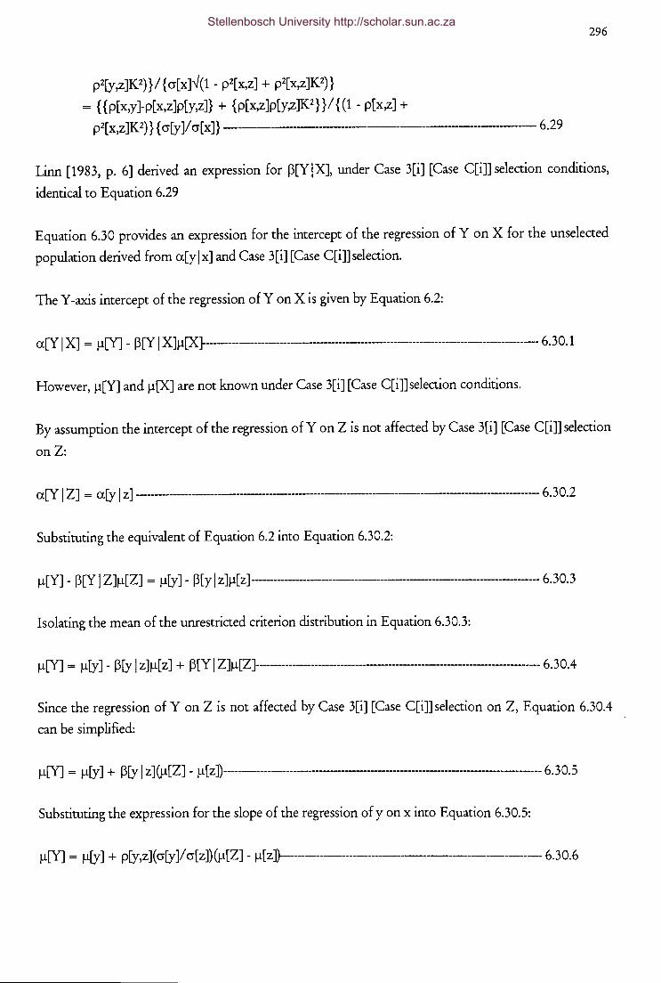
296
p2[y,z]K2)}/ { cr[x]--./(1 - p2[x,z] + p2[x,z]K2)}
= { {p[x,y]-p[x,z]p[y,z]} + {p[x,z]p[y,z]K2} }/ { (1 - p[x,z] +
p2[ x,z ]K 2)} { cr[y ]/ cr[ x ]} ----------------------------------------------- 6.29
Linn [1983, p. 6] derived an expression for p[YIXJ, under Case 3[i] [Case C[i]] selection conditions,
identical to Equation 6.29
Equation 6.30 provides an expression for the intercept of the regression of Y on X for the unselected
population derived from a[ylxJ and Case 3[i] [Case C[i]]selection.
The Y -axis intercept of the regression of Y on X is given by Equation 6.2:
a[Y I X] = ~[Y] - p[Y I X]~[X}--------------------------------------------------------------------------------------- 6.30.1
However, ~[Y] and ~[X] are not known under Case 3[i] [Case C[i]]selection conditions.
By assumption the intercept of the regression of Y on 2 is not affected by Case 3[i] [Case C[i]] selection
on2:
a[Y I 2] = a[y I z] ------------------------------------------------------------------------------------------------------------ 6.30.2
Substituting the equivalent of Equation 6.2 into Equation 6.30.2:
~[Y] - p [Y I 2]~[2] = ~[y] - p[y I z ]~[ z] ---------------------------------------------------------------------- 6. 3 0. 3
Isolating the mean of the unrestricted criterion distribution in Equation 6.30.3:
~[Y] = ~[y J - P[y I z J~[ z J + p[Y I 2]~[2]--------------------------------------------------------------------------- 6. 3 o .4
Since the regression of Y on 2 is not affected by Case 3[i] [Case C[i]] selection on 2, Equation 6.30.4
can be simplified:
~[Y] = ~[y] + p[y I z] (~[2] - ~[ z ])---------------------------------------------------------------------------- 6. 3 0. 5
Substituting the expression for the slope of the regression of yon x into Equation 6.30.5:
~[Y] = ~[y] + p[y,z] ( cr[y ]/ cr[ z ]) (~[2] - ~[ z ]}------------------------------------------------------------------- 6. 30.6
Stellenbosch University http://scholar.sun.ac.za
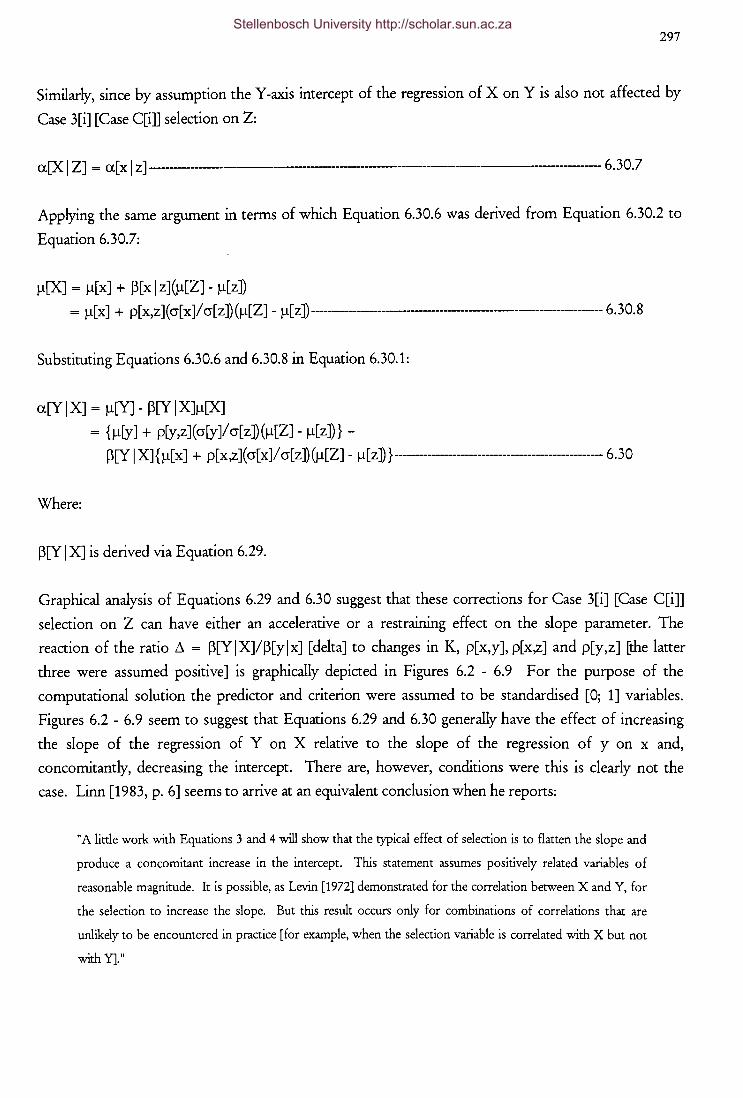
297
Similarly, since by assumption the Y -axis intercept of the regression of X on Y is also not affected by
Case 3[i] [Case C[i]] selection on Z:
a[X I Z] = a[x I z]----------------------------------------------------------- 6.30.7
Applying the same argument in terms of which Equation 6.30.6 was derived from Equation 6.30.2 to
Equation 6.30.7:
j..t[X] = j..t[x] + ~[xI z](J..t[Z]- J..t[z])
= j..t[ x] + p[ x,z] ( cr[ x ]/ cr[ Z ]) (J..t[ZJ - j..t[ Z ]) ---------------------------------------------------------------- 6. 30. 8
Substituting Equations 6.30.6 and 6.30.8 in Equation 6.30.1:
a[Y I X] = ).l[Y] - ~[Y I X]J..t[X]
= {J..t[y] + p[y,z](cr[y]/cr[z])(J..t[Z]- J..t[z])}-
~[Y I X]{J..t[x] + p[x,z](cr[x]/ cr[z])(J..t[Z]- J..t[z]) }-------------------------------------------------- 6.30
Where:
~[Y I X] is derived via Equation 6.29.
Graphical analysis of Equations 6.29 and 6.30 suggest that these corrections for Case 3[i] [Case C[i]]
selection on Z can have either an accelerative or a restraining effect on the slope parameter. The
reaction of the ratio~ = ~[YIXJ/~[ylxJ [delta] to changes inK, p[x,y], p[x,z] and p[y,z] [the latter
three were assumed positive] is graphically depicted in Figures 6.2 - 6.9 For the purpose of the
computational solution the predictor and criterion were assumed to be standardised [0; 1] variables.
Figures 6.2 - 6. 9 seem to suggest that Equations 6.29 and 6.30 generally have the effect of increasing
the slope of the regression of Y on X relative to the slope of the regression of y on x and,
concomitantly, decreasing the intercept. There are, however, conditions were this is clearly not the
case. Linn [1983, p. 6] seems to arrive at an equivalent conclusion when he reports:
"A little work with Equations 3 and 4 will show that the typical effect of selection is to flatten the slope and
produce a concomitant increase in the intercept. This statement assumes positively related variables of
reasonable magnitude. It is possible, as Levin [1972] demonstrated for the correlation between X andY, for
the selection to increase the slope. But this result occurs only for combinations of correlations that are
unlikely to be encountered in practice [for example, when the selection variable is correlated with X but not
withY]."
Stellenbosch University http://scholar.sun.ac.za
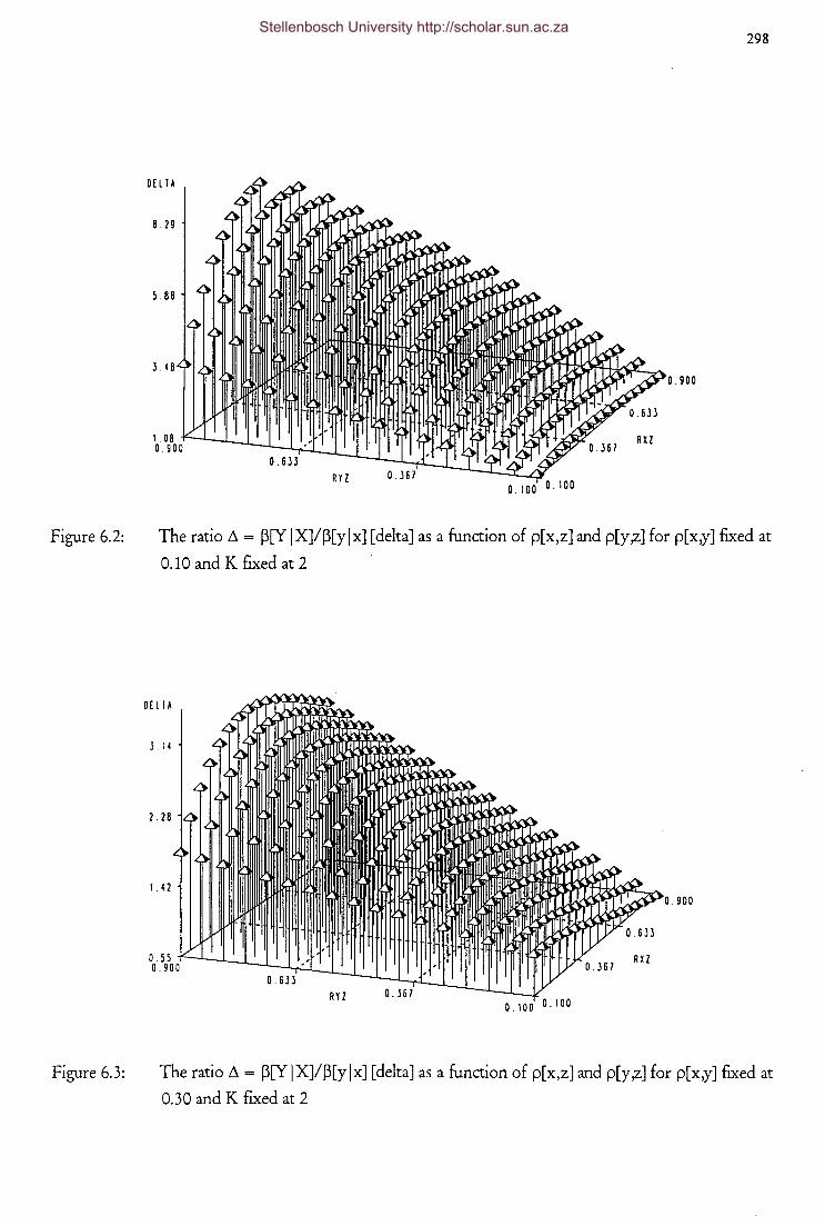
Figure 6.2:
Figure 6.3:
298
0.900
The ratio /j_ = p[Y JX]/p[yJx] [delta] as a function of p[x,z] and p[y,z] for p[x,y] fiXed at
0.10 and K fixed at 2
D [ L I A
3. 14
2.28
1 . 4 2 .900
0.100 0.100
The ratio /j. = p[Y JX]/p[y Jx] [delta] as a function of p[x,z] and p[y ,z] for p[x,y] fiXed at
0.30 and K fixed at 2
Stellenbosch University http://scholar.sun.ac.za
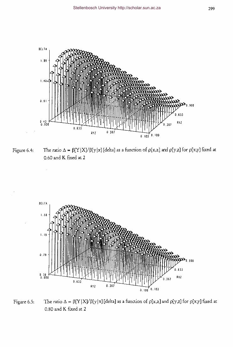
Figure 6.4:
Figure 6.5:
299
0[ l lA
1 . 8 9
1. 4 0
0. 9 1 .900
0.100 0.100
The ratio!).= p[Y IX]/p[yix] [delta] as a function of p[x,z] and p[y,z] for p[x,y] fixed at
0.60 and K fixed at 2
DEll A
1 60
1 . 19
0. 7 9
0.100 0.100
The ratio!).= p[Y IX]/p[yix] [delta] as a function of p[x,z] and p[y,z] for p[x,y] fixed at
0.80 and K fixed at 2
Stellenbosch University http://scholar.sun.ac.za

Figure 6.6:
Figure 6.7:
300
DELTA
17.94
12 32
6. 71 .900
RXZ
0.100 0.100
The ratio~= ~[YIXJ/~[ylxJ [delta] as a function of p[x,z]and p[y,z] for p[x,y] ftxed at
0.10 and K fixed at 4
.900
The ratio~ = ~[Y IXJ/~[ylxJ [delta] as a function of p[x,z] and p[y ,z] for p[x,y] ftxed at
0.30 and K fixed at 4
Stellenbosch University http://scholar.sun.ac.za

Figure 6.8:
Figure 6.9:
301
DEll A
J. 44
7. J1
1 . J 1
RXZ 0. 75 )-'---L_-L..:.-;~a~~~~s1tTI~J[jJI 0.900
RYl 0.100 0.100
The ratio~= p[Y IXJ/p[ylxJ [delta] as a function of p[x,z] and p[y,z] for p[x,y] fixed at
0.60 and K fixed at 4
.900
The ratio~= P[YIXJ/p[ylxJ [delta] as a function of p[x,z] and p[y,z] for p[x,y] fixed at
0.80 and K fixed at 4
Stellenbosch University http://scholar.sun.ac.za
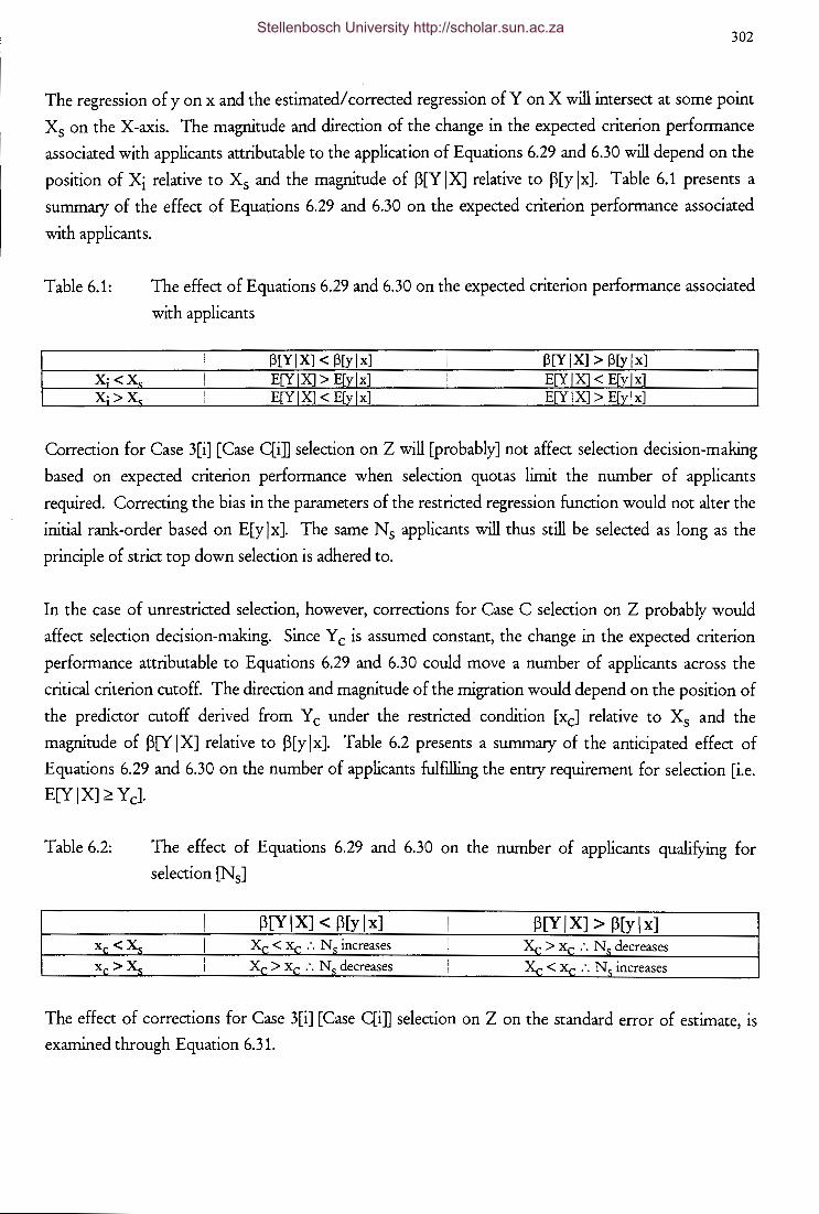
302
The regression of y on x and the estimated/ corrected regression of Y on X will intersect at some point
Xs on the X -axis. The magnitude and direction of the change in the expected criterion performance
associated with applicants attributable to the application of Equations 6.29 and 6.30 will depend on the
position of Xi relative to Xs and the magnitude of ~[Y IXJ relative to ~[y lx]. Table 6.1 presents a
summary of the effect of Equations 6.29 and 6.30 on the expected criterion performance associated
with applicants.
Table 6.1:
X·<X~ X·>X.,
The effect of Equations 6.29 and 6.30 on the expected criterion performance associated
with applicants
I ~[YIXJ < ~[ylxJ I ~[YIXJ > ~[ylxJ ! I
I E[Y IX]> E[yJx] I E[Yl X] < E[yJ x] I E[Y IX]< E[ylx] I E[YIX] > E[ylx] i
Correction for Case 3[i] [Case Qi] selection on Z will [probably] not affect selection decision-making
based on expected criterion performance when selection quotas limit the number of applicants
required. Correcting the bias in the parameters of the restricted regression function would not alter the
initial rank-order based on E[ylx]. The same Ns applicants will thus still be selected as long as the
principle of strict top down selection is adhered to.
In the case of unrestricted selection, however, corrections for Case C selection on Z probably would
affect selection decision-making. Since Y c is assumed constant, the change in the expected criterion
performance attributable to Equations 6.29 and 6.30 could move a number of applicants across the
critical criterion cutoff. The direction and magnitude of the migration would depend on the position of
the predictor cutoff derived from Y c under the restricted condition [xcJ relative to Xs and the
magnitude of ~[Y I X] relative to ~[y I x]. Table 6.2 presents a summary of the anticipated effect of
Equations 6.29 and 6.30 on the number of applicants fulfilling the entry requirement for selection [i.e.
E[Y I X] ~ y cJ.
Table 6.2:
Xc<Xs
Xc>Xs
The effect of Equations 6.29 and 6.30 on the number of applicants qualifying for
selection [N sJ
I ~[YIXJ < ~[ylxJ I ~[YIXJ > ~[ylxJ I Xc < Xc :. N 5 increases ! Xc > Xc :. N s decreases I Xc > ~c :. N 5 decreases I Xc < Xc :. N 5 increases I I
The effect of corrections for Case 3[i] [Case Qi] selection on Z on the standard error of estimate, is
examined through Equation 6.31.
Stellenbosch University http://scholar.sun.ac.za

303
The standard error of estimate for the unrestricted applicant population is given by the square root of
Equation 6.5:
cr[Y I X] = cr[Y]--1(1 - p2[X,Y] _______ , __ , ---------------------------------- 6.31.1
However, p[X,Y] and cr[Y] are both unknown under Case 3[i] [Case C[i]] conditions
By assumption the regression ofY on Z is not effected by Case 3[i] [Case C[i]]selection on Z:
~[Y I Z] = ~[y I z] -------------------------------------------------------------------------------------------------- 6. 31.2
Substituting the appropriate equivalent of Equation 6.3 into Equation 6.31.2:
p[Y ,Z] ( cr[Y]/ cr[Z]) = p[y ,z ]( cr[y ]/ cr[ z ])----------------------------------------------------------------------------- 6. 31.3
Isolating the term p[Y,Z] in Equation 6.31.3:
p[Y ,Z] = p[y,z] ( ( cr[y ]cr[Z]) I ( cr[ z ]cr[Y]) }------------------------------------------------------------------------ 6. 31.4
Furthermore, by assumption the criterion variance conditional on Z is also not affected by Case 3[i]
[Case C[i]] selection on Z:
cr[yl~=cr[YIZJ------------------------------------------------------6.31.5
Substituting the appropriate equivalent of Equation 6.5 in Equation 6.31.5:
cr2[y ]( 1 - p2[y,z]) = cr2[Y]( 1 - p2[Y,Z]) ------------------------------------------------------------------ 6.31.6
Substituting Equation 6.31.4 in Equation 6.31.6:
cr2[y](1- p2[y,z]) = cr2[Y](1- {p2[y,z]((cr2[y]cr2[Z])/(cr2[z]cr2[Y]))})
= cr2[YJ _ p2[y ,z ]cr2(y ]( cr2[Z]/ cr2[ z ])
= cr2[Y] - p2[y ,z ]cr2[y ]K 2-------------------------------------------------------------------- 6. 31.7
Where, K = cr[Z]/ cr[ z]
Isolating the unrestricted criterion variance term in Equation 6.31.7:
Stellenbosch University http://scholar.sun.ac.za

cr2[YJ = cr2[y](1 _ p2[y,z]) + p2[y,z]cr2[y]K2
= cr2[y](1- p2[y,z] + p2[y,z]K2)------------------------------------ 6.31.8
Substituting Equation 6.31.8 and the square of Equation 3.5 in Equation 6.31.1:
cr2[Y I X] = cr2[Y](1 - p2[X,Y]
Thus:
= cr2[y](1- p2[y,z] + p2[y,z]K2){1- {{(p[x,y]-p[x,z]p[y,z] +
(p[x,z]p[y,z]K2)}/{"(1- p2[x,z] + p2[x,z]K2)"(1- p2[y,z] + p2[y,z]K2)}}2}
= cr2[y](1 - p2[y,z] + p2[y,z]K2) - { (p[x,y]-p[x,z]p[y ,z] +
(p[ x,z ]p[y,z ]K 2)2} I ( 1 - p2[x,z] + p2[ x,z ]K 2)------------------------------------------------ 6.31. 9
cr[YIXJ = cr[y]"(l- p2[y,z] + p2[y,z]K2)- (p[x,y]-p[x,z]p[y,z] +
(p[ x,z ]p[y,z ]K 2) I" ( 1 - p2[ x,z] + p2[ x,z ]K 2}--------------------------------------------------------- 6.31
304
Graphical analysis suggests the effect of Equation 6.31 on the standard error of estimate to vary as a
function of p[x,y], p[x,z], p[y,z] and K [i.e. the selection/truncation ratio]. Figures 6.10 - 6.17 depict
the reaction of the ratio ~ = cr[Y I X]/ cr[y I x] [Delta] to changes in p[ x, y ], p[x,z ], p[y ,z] md K.
For the purpose of the analysis the predictor and criterion were assumed to be standardised [0; 1]
variables. Figures 6.10- 6.17 seem to suggest that Equation 6.31 generally has the effect of reducing
the standard error of estimate. There are, however, conditions were this is clearly not the case. An
increase in the standard error of estimate seem to occur at low values of p[x,z] rombined with high
values on p[y,z].
An analysis of the effect of corrections for Case 3[i] [Case C[i]] selection on Z, on selection decision
making based on the conditional probability of success, should focus on the relative position of Y c in
the conditional criterion distribution. Since the critical criterion cutoff value, Y 0 is defined on a scale
unaffected by [systematic and/ or random] measurement error, the relative position of Y c in the
conditional criterion distribution depends on the reaction of both the expected criterion performance
and the standard error of estimate to corrections for Case 3[i] [Case C[i]] selection on Y. A factor
complicating the issue, however, is the complexity of the reaction of both the expected criterion
performance and the standard error of estimate to corrections for Case 3[i] [Case C[i]] selection on Y
over the space defined by p[ x,y ], p[y,z ], p[ x,z] and K. Since p[Y I X] can be either bigger or smaller than
p[y I x] and cr[Y I X], similarly, can be either bigger or smaller than cr[y I x ], at least four possible
outcomes have to be considered. The probabilities of each of these four possible outcomes occurring
are not equal.
Stellenbosch University http://scholar.sun.ac.za

305
DEllA
1.495
1 1 7)
0. 85 1 0. 9 00
0.)67 RXZ
RYl 0.100 0.100
Figure 6.10: The ratio !:1 = cr[Y I X]/ cr[y I x] [Delta], under Case 3[i] [Case C[i]] restriction of range as
a function of p[x,z] and p[y,z] for p[x,y] frxed at 0.10 and K fixed at 2
0 [ l l A
0. 9 00
0.100 0.100
Figure 6.11: The ratio !:1 = cr[YIXJ/cr[ylxJ [Delta], under Case 3[i] [Case C[i]]restriction of range as
a function of p[x,z] and p[y,z] for p[x,y] fixed at 0.30 and K fixed at 2
Stellenbosch University http://scholar.sun.ac.za
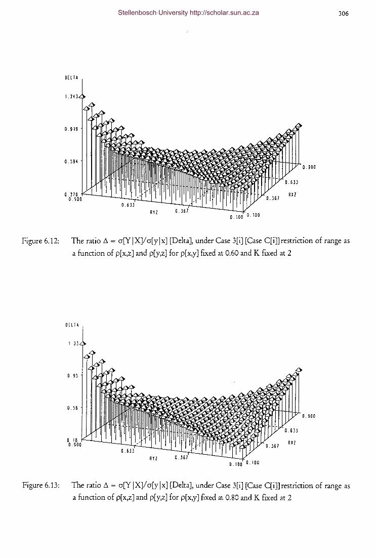
306
0£ l TA
1. 24J
0.919
0. 59 4 0.900
0. 270 --_,_-L~~r~~~~~;D1~~~Wl 0.900 0.633
RYl 0.367
0.367 RXl
0.100 0.100
Figure 6.12: The ratio .1 = cr[YjX]/cr[yjx] [Delta], under Case 3[i] [Case C[i]]restriction of range as
a function of p[x,z] and p[y,z] for p[x,y] fixed at 0.60 and K fixed at 2
0 [ l I A
1 . 3 3
0.95
0.56
0.900
0.100 0.100
Figure 6.13: The ratio .1 = cr[Y I X]/cr[yjx] [Delta], under Case 3[i] [Case C[i]] restriction of range as
a function of p[x,z] and p[y,z] for p[x,y] fixed at 0.80 and K fixed at 2
Stellenbosch University http://scholar.sun.ac.za

307
0[ ll A
2.29
1. 6 2
0.95 0.900
0.367 RXZ
RYl 0.100 0.100
Figure 6.14: The ratio 6 = cr[Y I X]/ cr[y I x] [Delta], under Case 3[i] [Case C[i]] restriction of range as
a function of p[x,z] and p[y,z] for p[x,y] fiXed at 0.10 and K fixed at 4
0 [ L 1 A
0.900
0.100 0.100
Figure 6.15: The ratio 6 = cr[Y I X]/cr[ylxJ [Delta], under Case 3[i] [Case C[i]]restriction of range as
a function of p[x,z] and p[y,z] for p[x,y] fiXed at 0.30 and K fixed at 4
Stellenbosch University http://scholar.sun.ac.za

308
DELIA
2.26
1. 55
0.85
RXZ
0.100 0.100
Figure 6.16: The ratio~= cr[YIXJ/cr[ylxJ [Delta], under Case 3[i] [Case C[i]]restriction of range as
a function of p[x,z] and p[y,z] for p[x,y] fixed at 0.60 and K fixed at 4
Figure 6.17: The ratio ~ = cr[Y I X]/ cr[y I x] [Delta], under Case 3[i] [Case C[i]] restriction of range as
a function of p[x,z] and p[y,z] for p[x,y] fixed at 0.80 and K fixed at 4
Stellenbosch University http://scholar.sun.ac.za

309
The most likely outcome seems to be an increase in slope combined with a decrease in the standard
error of estimate. A highly unlikely outcome, on the other hand, seems to be a decrease in slope
combined with an increase in the standard error of estimate. The position of Xi relative to the point Xs
where the corrected and uncorrected regression lines intersect [i.e. E[Y I X = Xs] = E[y I x = XsJ], furthermore needs to be considered. An analysis of the effect of corrections for Case 3[i] [Case C[i]]
selection on Z, on selection decision making based on the conditional probability of success, would
therefore have to reckon with the eight possible conditions depicted in Table 6.3.
Table 6.3: The eight possible conditions affecting the effect of corrections for Case 3[i] [Case C[i]]
selection on Z on selection decision making based on the conditional probability of
success
~[YIXl < ~[ylxl ~[YIXl > ~[ylxl X·<X_s I
cr[Y I X] < cr[y I x] ? I ? P decreases
cr[Y I X] > cr[y I x] P increases ! P decreases
The three dimensions defining Table 6.3 collectively determine whether the change in the expected
criterion performance and the change in the variance of the conditional criterion distribution exert a
concerted or an antagonistic influence on the conditional probability of success. In the latter case, with
the two processes opposing each other, the effect on the conditional probability of success is somewhat
more difficult to fathom since it depends on which one of the two processes dominate and thus on Xi '
[more specifically, the extent to which Xi deviates from XsJ. Table 6.3 depicts the anticipated effect of
Equations 6.29, 6.30 and 6.31 on the conditional probability of success
Correction for Case 3[i] [Case Qi] selection on Z will [probably] not affect selection decision-making
based on conditional probability of success when selection quotas limit the number of applicants
required. The initial rank-order based on P[y ~ Y c I x] will not be altered by Equations 6.29, 6.30 and
6.31. The same Ns applicants will therefore still be selected as long as the principle of strict top down
selection is still adhered to.
In the case of unrestricted selection, however, decisions will be affected. Since Y c is assumed constant,
the change in the conditional probability of success attributable to Equations 6.29, 6.30 and 6.31 would
probably move a number of applicants across the critical criterion cutoff as. The direction of the
migration would depend on the three dimensions of Table 6.3. Either an increase or a decrease in the
number of applicants selected could therefore occur
Stellenbosch University http://scholar.sun.ac.za
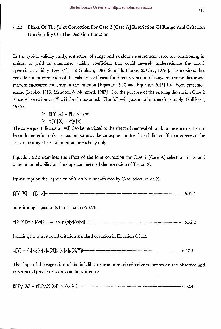
310
6.2.3 Effect Of The Joint Correction For Case 2 [Case A] Restriction Of Range And Criterion
Unreliability On The Decision Function
In the typical validity study, restriction of range and random measurement error are functioning in
unison to yield an attenuated validity coefficient that could severely underestimate the actual
operational validity [Lee, Millar & Graham, 1982; Schmidt, Hunter & Uny, 1976;]. Expressions that
provide a joint correction of the validity coefficient for direct restriction of range on the predictor and
random measurement error in the criterion [Equation 3.10 and Equation 3.13] had been presented
earlier [Bobko, 1983; Mendoza & Mumford, 1987]. For the purpose of the ensuing discussion Case 2
[Case A] selection on X will also be assumed. The following assumption therefore apply [Gulliksen,
1950]:
~ ~[YIXJ = ~[ylx]; and
~ cr[Y I X] = cr[y I x]
The subsequent discussion will also be restricted to the effect of removal of random measurement error
from the criterion only. Equation 3.2 provides an expression for the validity coefficient corrected for
the attenuating effect of criterion unreliability only.
Equation 6.32 examines the effect of the joint correction for Case 2 [Case A] selection on X and
criterion unreliability on the slope parameter of the regression of Ty on X.
By assumption the regression of Y on X is not affected by Case selection on X:
~[Y I X] = ~[y I x]------------------------------------------------------------------------------------------------- 6.32.1
Substituting Equation 6.3 in Equation 6.32.1:
p[X, Y] ( cr[Y]/ cr[X]) = p[ x, y ]( cr[y ]/ cr[ x ]) --------------------------------------------------------------------------- 6. 3 2.2
Isolating the unrestricted criterion standard deviation in Equation 6.32.2:
cr[Y] = (p[ x,y ]cr[y ]cr[X]) I ( cr[ x ]p[X, Y] ----------------------------------------------------------------------- 6.3 2.3
The slope of the regression of the infallible or true unrestricted criterion scores on the observed and
unrestricted predictor scores can be written as:
~[T y I X] = p[T y ,X]( cr[T y ]/ cr[X])------------------------------------------------------------------------------ 6. 3 2. 4
Stellenbosch University http://scholar.sun.ac.za

Substituting Equation 3.2 and Equation 2.16 in Equation 6.32.4:
~[Ty I X] = (p[X,Y]/ .V Ptt y) ( .V Ptt ycr[Y]/ cr[X]
= (p[X,Y]) ( cr[Y]/ cr[X]) ------------------------------------------------------ 3.3 2.5
Substituting Equation 3.32.3 in Equation 3.32.5:
~[Ty I X] = (p[X,Y]) { (p[x,y ]cr[y]cr[X]/ (cr[x]p[X,Y])} (1/ cr[X])
= p[ x,y ]( cr[y ]/ cr[ x ])
= ~[y I X]---------------------------------------------------------------------------------------- 6. 3 2
311
Equation 6.32 indicates that the slope parameter is not affected by the joint correction for Case 2 [Case
A] selection on X and criterion unreliability.
Equation 6.33 examines the effect of the joint correction for Case 2 [Case A] selection on X and
criterion unreliability on the intercept parameter of the regression of Ty on X.
By assumption the regression of the unrestricted criterion on the unrestricted predictor is not affected
by Case 2 [Case A] selection on X:
a [Y I X] = a[y I x] ----------------------------------------------------------------------------------------------------------- 6. 3 3 .1
Based on Equation 6.2, the intercept of the regression of the unrestricted criterion true scores on the
unrestricted, observed predictor can be expressed as:
a[Ty I X] = J.![Ty] - ~[Ty I X]J.![X] -------------------------------------------------------------------------------- 6.33.2
However, since, J.![Ty] = J.![Y - E] = J.![Y] - J.![E] = J.![Y], Equation 6.33.2 can be rewritten as:
a[Ty I X] = J.![Y] - ~[Ty I XJJ.![XJ----------------------------------------------------------------------------------- 6.33.3
Combining Equation 6.32 with the assumption that the regression of Yon X is not affected by Case 2
[Case A] selection on X, implies that Equation 6.33.3 can be rewritten as:
a[Ty I X] = J.![Y] - ~[Y I X]J.![X]
= a[y I x] --------------------------------------------------------------------------------------------------------- 6. 3 3
Stellenbosch University http://scholar.sun.ac.za

312
The intercept parameter is therefore also not affected by the joint correction for Case 2 [Case A]
selection on X and criterion unreliability.
Equations 6.32 and 6.33 imply that the expected criterion performance associated with applicants will
not be affected by the simultaneous removal of random measurement error from the criterion and the
reversal of explicit Case 2 selection on the predictor. Selection decision-making will consequently not
be affected by the simultaneous removal of random measurement error from the criterion and the
reversal of explicit Case 2 selection on the predictor, irrespective of whether selection quotas apply or
not.
Equation 6.34 examines the effect of the joint correction for Case 2 [Case A] selection on X and
criterion unreliability on the standard error of estimate of the regression of Ty on X.
Based on Equation 6.5, the unrestricted true score criterion standard deviation conditional on the
unrestricted, observed predictor score can be expressed as:
cr[T y I X] = cr[T y ]-..J ( 1 - p2[T y ,x]) -------------------------------------------------------------------------- 6. 34.1
Substituting Equation 2.16 in Equation 6.34.1:
cr[T y I X] = ( -.J Ptt ys[Y]) -.J ( 1 - p2[T y ,x] --------------------------------------------------------------------- 6. 3 4.2
By assumption the regression of Y on X is not affected by Case selection on X:
p [Y I X] = p [y I X]--------------------------------------------------------------------------------------------------------- 6. 3 4. 3
Substituting Equation 6.3 in Equation 6.34.3:
p[X, Y] ( cr[Y]/ cr[X]) = p[ x, y ]( cr[y ]/ cr[ x ]) ------------------------------------------------------- 6. 34.4
Isolating the unrestricted, observed criterion standard deviation:
cr[Y] = (p[ x,y ]cr[y ]cr[X]) I ( cr[ x ]p[:X, Y]) ---------------~------------------------------------------- 6. 34. 5
However, Equation 3.4 provides an expression for the validity coefficient corrected for Case 2 [Case A]
selection::
p[X,Y] = (cr[X]p[x,y])/-..J(cr2[X]p2[x,y] + cr2[x]- cr2[x]p2[x,y]----------------------------------------- 6.34.6
Stellenbosch University http://scholar.sun.ac.za
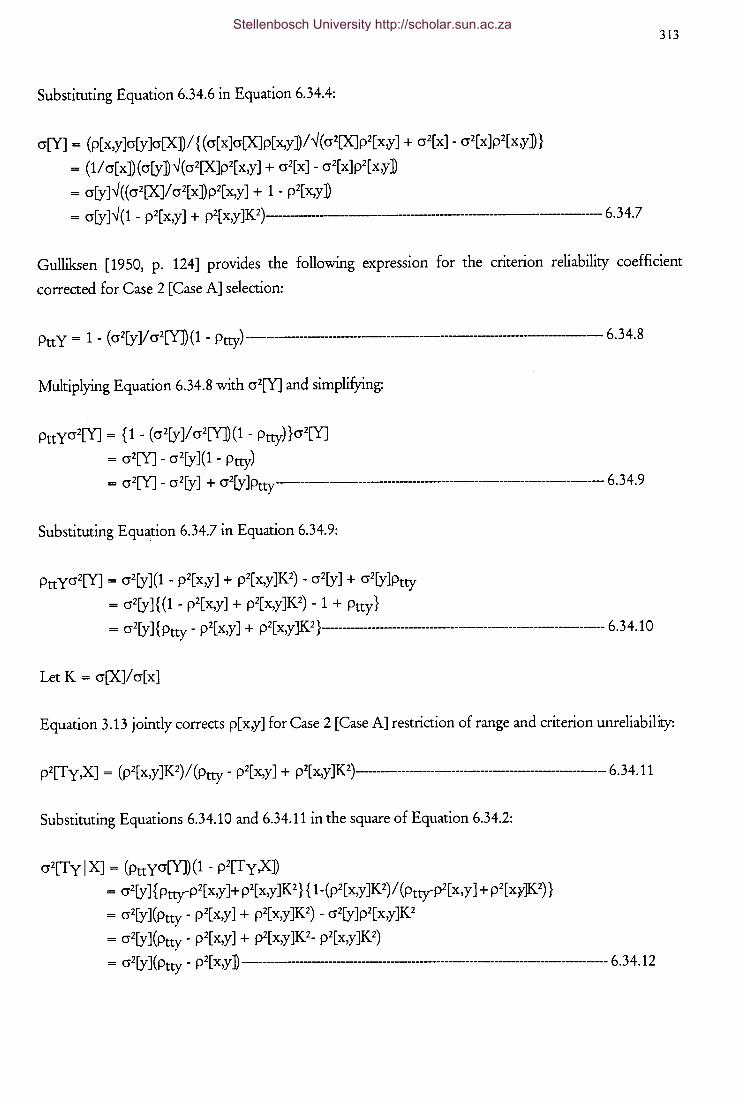
Substituting Equation 6.34.6 in Equation 6.34.4:
cr[Y] = (p[x,y]cr[y]cr[X])I{(cr[x]cr[X]p[x,y]lv'(cr2[X]p2[x,y] + cr2[x]- cr2[x]p2[x,y]}
= (11cr[x])(cr[y]v'(cr2[X]p2[x,y] + cr2[x]- cr2[x]p2[x,y]
= cr[y ]v' ( ( cr2[X]I cr2[x ]) p2[ x,y] + 1 - p2[ x,y]
= cr[y]v'(1- p2[x,y] + p2[x,y]K2)------------------------------------------------------ 6.34.7
313
Gulliksen [1950, p. 124] provides the following expression for the criterion reliability coefficient
corrected for Case 2 [Case A] selection:
Ptt y = 1 - ( cr2[y ]/ cr2[Y]) (1 - Ptty) ------------------------------------------------------------------- 6.34.8
Multiplying Equation 6.34.8 with cr2[Y] and simplifying:
PttYcr2[Y] = {1- (cr2[y]lcr2[Y](1- Ptty)}cr2[Y]
= cr2[YJ- cr2[y ](1 - Ptty)
= cr2[YJ _ cr2[y] + cr2(y ]Ptty--------------------------------------------------------------------- 6. 34.9
Substituting Equation 6.34.7 in Equation 6.34.9:
PttYcr2[YJ = cr2[y](1 - p2[x,y] + p2[x,y]K2)- cr2(y] + cr2(yJPtty
= cr2(y]{(1- p2[x,y] + p2[x,y]K2)- 1 + Ptty}
= cr2(y J { Ptty - p2[ x,y] + p2[ x,y ]K 2 }------------------------------------------------------------------- 6. 34.10
Let K = cr[X]I cr[ x]
Equation 3.13 jointly corrects p[x,y] for Case 2 [Case A] restriction of range and criterion unreliability:
p2[Ty,X] = (p2[ x,y ]K 2) I (Ptty - p2[ x,y] + p2[ x,y ]K2)----------------------------------------------------------- 6.34.11
Substituting Equations 6.34.10 and 6.34.11 in the square of Equation 6.34.2:
cr2[Ty I X]= (puycr[Y])(1 - p2[Ty ,X] = crz[y ]{ Puy-p2[ x,y ]+ p2[ x,y ]K 2} { 1-(p2[ x,y ]K2) I (Pny-P2[ x, y] + p2[ xy]IQ)}
= cr2[y](Ptty _ p2[x,y] + p2[x,y]K2) _ cr2(y]p2[x,y]K2
= cr2[y](Ptty _ p2[x,y] + p2[x,y]K2- p2[x,y]K2)
= cr2[y] (Ptty - p2[ x,y] ------------------------------------------------------------------------------ 6.34.12
Stellenbosch University http://scholar.sun.ac.za
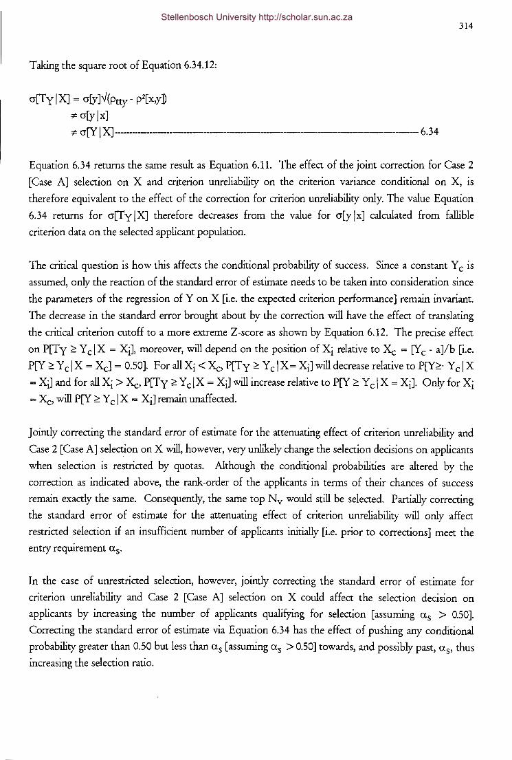
Taking the square root of Equation 6.34.12:
cr[Ty I X] = cr[y ]~ (Ptty - p2[ x,y]
:;t: cr[ylxJ
:;e cr[Y I X]------------------------------------------------------------------------ 6.34
314
Equation 6.34 returns the same result as Equation 6.11. The effect of the joint correction for Case 2
[Case A] selection on X and criterion unreliability on the criterion variance conditional on X, is
therefore equivalent to the effect of the correction for criterion unreliability only. The value Equation
6.34 returns for cr[Ty IXJ therefore decreases from the value for cr[y lxJ calculated from fallible
criterion data on the selected applicant population.
The critical question is how this affects the conditional probability of success. Since a constant Y c is
assumed, only the reaction of the standard error of estimate needs to be taken into consideration since
the parameters of the regression of Y on X [i.e. the expected criterion performance] remain invariant.
The decrease in the standard error brought about by the correction will have the effect of translating
the critical criterion cutoff to a more extreme Z-score as shown by Equation 6.12. The precise effect
on P[T y :2: Y c I X = Xi], moreover, will depend on the position of Xi relative to Xc = [Y c - a ]/b [i.e.
P[Y :2: Y c I X = XcJ = 0.50]. For all Xi < Xc, P[Ty :2: Y c I X= Xi] will decrease relative to P[Y:2:· Y c I X
= Xi] and for all Xi > Xc, P[T y :2: Y c I X = Xi] will increase relative to P[Y :2: Y c I X = Xi]. Only for Xi
= Xc, will P[Y :2: Y c I X = Xi] remain unaffected.
Jointly correcting the standard error of estimate for the attenuating effect of criterion unreliability and
Case 2 [Case A] selection on X will, however, very unlikely change the selection decisions on applicants
when selection is restricted by quotas. Although the conditional probabilities are altered by the
correction as indicated above, the rank-order of the applicants in terms of their chances of success
remain exactly the same. Consequently, the same top Nv would still be selected. Partially correcting
the standard error of estimate for the attenuating effect of criterion unreliability will only affect
restricted selection if an insufficient number of applicants initially [i.e. prior to corrections] meet the
entry requrrement as.
In the case of unrestricted selection, however, jointly correcting the standard error of estimate for
criterion unreliability and Case 2 [Case A] selection on X could affect the selection decision on
applicants by increasing the number of applicants qualifying for selection [assuming as > 0.50].
Correcting the standard error of estimate via Equation 6.34 has the effect of pushing any conditional
probability greater than 0.50 but less than as [assuming as > 0.50] towards, and possibly past, as, thus
increasing the selection ratio.
Stellenbosch University http://scholar.sun.ac.za

315
6.3 CONCLUDING COMMENTS
The foregoing results apply only for the joint correction for criterion unreliability and Case 2 [Case A]
selection on X. Analogous joint corrections would be possible, however, such as corrections for:
~ both criterion and predictor unreliability [i.e. working with E[Tx I X] instead of X]
and Case 2 [Case A] selection on X;
~ criterion unreliability and Case C selection on C; and
~ both criterion and predictor unreliability and Case C selection on Z;
The effect of these joint corrections on the information on applicants relevant to the strategy matrix
has not been examined. It would almost certainly differ from the results reported here.
In chapter 5 the question was raised whether statistical corrections for random measurement error
and/ or various forms of restriction of range affect statistical significance testing on the corrected
correlation/validity coefficient, and if so, in what way. An equivalent question could and should be
raised with regards to the parameters of the regression of the criterion on the predictor.
No attempt is made in this study to formally examine this issue. The hypothesis is, however, put
forward, that, as . in the case of the uncorrected correlation coefficient and the uncorrected slope
coefficient, the exceedence probabilities associated with the corrected correlation coefficient and the
corrected slope coefficient would coincide.
6.4 SUMMARY
Chapter 6 presented the logic underlying selection decision making so as to establish the necessary
theoretical foundation for the subsequent analysis. It was then argued that the logic underlying the
corrections for restriction of range and/ or criterion unreliability applied to the validity coefficient
should be extended to the decision rule in terms of which applicants are screened for employment.
The subsequent analyses derived analytical expressions indicating the effects of applying correction for
restriction of range and/ or criterion unreliability to the slope, intercept and conditional variance
parameters of the regression of Y on X. The effect of changes to these parameters on actual selection
decision-making was then investigated.
Stellenbosch University http://scholar.sun.ac.za
CHAPTER7
CONCLUSIONS AND RECOMMENDATIONS FOR FURTHER RESEARCH
The first objective of the ensuing discussion is to review the reasoning in terms of which the necessity
and significance of the foregoing research was justified, to provide a concise description of the nature
of the analyses, and to present a summary of the findings of the analyses. Following on from this, the
second objective of the discussion is to present recommendations on further research required.
7.1 CONCLUSIONS
7.1.1 Reviewing The Necessity And Significance Of The Research
Selection, as it is traditionally interpreted, represents a critical human resource intervention in any
organisation in as far as it regulates the movement of employees into, through and out of the
organisation. As such selection thus firstly represents a potentially powerful instrument through which
the human resource function can add value to the organisation [Boudreau, 1983b; Boudreau & Berger,
1985a; Cascio, 1991b; Cranshaw & Alexander, 1985]. Selection, however, also represents a relatively
visible mechanism through which access to employment opportunities are regulated. Because of this
latter aspect, selection, more than any other human resource intervention, has been singled out for
intense scrutiny from the perspective of fairness and affirmative action [Arvey & Faley, 1988; Milkovich
& Boudreau, 1994;]. Two basic criteria are implied in terms of which selection procedures need to be
evaluated, namely efficiency and equity [Milkovich & Boudreau, 1994]. The quest for efficient and
equitable selection procedures requires periodic psychometric audits to provide the feedback needed to
refine the selection procedure towards greater efficiency and to provide the evidence required to
vindicate the organisation should it be challenged in terms of anti-discriminatory legislation. According
to the Guidelines for the validation and use of personnel selection procedures [Society for Industrial
Psychology, 1992], the Principles for the validation and use of personnel selection procedures [Society
for Industrial and Organisational Psychology, 1987] and the Kleiman and Faley [1985] review of
selection litigation, such a psychometric audit of a selection procedure would require the human
resource function to demonstrate that:
~ the selection procedure has its foundation in a scientifically credible performance
theory;
~ the selection procedure constitutes a business necessity; and
Stellenbosch University http://scholar.sun.ac.za
317
)> the manner in which the selection strategy combines applicant information can be
considered fair.
The empirical evidence needed to meet the aforementioned burden of persuasion is acquired through a
simulation of the actual selection procedure on a sample taken from the applicant population. Internal
and external validity constitute two criteria in terms of which the credibility and convincingness of the
evidence produced by such a simulation would be evaluated. The following two crucial questions are
thereby indicated:
)> to what extent can the researcher be confident that the research evidence produced
by the selection simulation corroborates the latent structure/ nomological network
postulated by the research hypothesis within the limits set by the specific conditions
characterising the simulation?; and
)> to what extent can the researcher be confident that the conclusions reached on the
simulation will generalise or transport to the area of actual application?
The conditions under which selection procedures are typically simulated and those prevailing at the
eventual use of a selection procedure normally differ to a sufficient extent to challenge the
transportability of the validation research evidence. Nevertheless, given the applied nature of selection
validation research, an attempt at generalisation is unavoidable. According to Stanley and Campbell
[1963] external validity is threatened by the potential specificity of the demonstrated effect of the
independent variable[s] to particular features of the research design not shared by the area of
application. In selection validation research the effect of the [composite] independent variable on the
criterion is captured by the validity coefficient. The area of application is characterised by a sample of
actual applicants drawn from the applicant population and measured on a battery of fallible predictors
with the aim of "estimating their actual contribution to the organisation [i.e. ultimate criterion scores]
and not an indicator of it attenuated by measurement error" [Campbell, 1991, p. 694].The estimate is
derived from a weighted linear composite of predictors derived from a representative sample of the
actual applicant population. The question regarding external validity, in the context of selection
validation research, essentially represents an inquiry into the unbiasedness of the parametric validity
coefficient estimate [i.e. the sample statistic] obtained through the validation study. The parameter of
interest is the correlation coefficient obtained when the sample weights derived from a representative
sample are applied to the applicant population and the weighted composite score is correlated with the
criterion, unattenuated by measurement error, in the population [Campbell, 1991 ]. The preceding
discussion clearly identifies the term "applicant population" to be of central importance should a
sufficiently precise depiction of the area of actual application be desired. The term "applicant
population", however, even if defined as the population to which a selection procedure will be applied,
still has an annoying impreciseness to it. A more unambiguous definition of the term, however,
depends on how the selection procedure is positioned relative to any selection requirements already in
Stellenbosch University http://scholar.sun.ac.za

318
use [i.e. whether it would replace, follow on, or be integrated with current selection requirements]. This
issue, moreover, is linked to the question regarding the appropriate decision alternative with which to
compare the envisaged selection procedure when examining its strategic merit.
In the context of selection validation research, given the aforementioned depiction of the area of
application, the following specific threats to external validity can be identified [Campbell, 1991; Lord &
Novick, 1968; T abachnick & Fidell, 1989]:
~ the extent to which the actual or operationalised criterion contains random
measurement error;
~ the extent to which the actual or operationalised criterion is systematically biased;
i.e. the extent to which the actual criterion is deficient and/ or contaminated [Blum
&Naylor, 1968];
~ the extent to which the validation sample is an unrepresentative, biased, sample
from the applicant population in terms of homogeneity and specific attributes [e.g.
motivation, knowledge/ experience];
~ the extent to which the sample size and the ratio of sample size to number of
predictors allow capitalisation on chance and thus overfitting of the data.
The conditions listed as threats all affect the validity coefficient [Campbell, 1991; Crocker & Algina,
1986; Dobson, 1988; Hakstian, Schroeder & Rogers, 1988; Lord & Novick, 1968; Mendoza &
Mumford, 1987; Messick, 1989; Olsen & Becker, 1983; Schepers, 1996], some consistently exerting
upward pressure, others downward pressure and for some the direction of influence varies. It thus
follows that, to the extent that the aforementioned threats operate in the validation study but do not
apply to the actual area of application, the obtained validity coefficient cannot, without formal
consideration of these threats, be generalised to the actual area of application. Thus, the obtained
validity coefficient cannot, without appropriate corrections, be considered an unbiased estimate of the
actual validity coefficient of interest.
Statistical corrections to the validity coefficient are generally available to estimate the validity coefficient
that would have been achieved had it been calculated under the condition that characterise that area of
actual application [Gulliksen, 1950; Pearson, 1903; Thorndike, 1949]. Campbell [1991, p. 701]
consequently recommends that:
If the point of central interest is the validity of a specific selection procedure for predicting performance over
a relatively long time period for the population of job applicants to follow, then it is necessary to correct for
restriction of range, criterion unreliability, and the fitting of error by differential predictor weights. Not to do
so is to introduce considerable bias into the estimation process.
Stellenbosch University http://scholar.sun.ac.za

319
The remainder of the argument in terms of which a selection procedure is developed and justified
could, however, also be biased by any discrepancy between the conditions under which the selection
procedure is simulated and those prevailing during the eventual use of the selection procedure.
Relatively little concern, however, seem to exist for the transportability of the decision function derived
from the selection simulation and descriptions/ assessments of selection decision utility and fairness.
This seems to be a somewhat strange state of affairs. The external validity problems of validation
designs are reasonably well documented [Barrett, Philips & Alexander, 1981; Cook, Campbell &
Peracchio, 1992; Guion & Cranny, 1982; Sussmann & Roberson, 1986]. It is therefore not as if the
psychometric literature is unaware of the problem of generalising validation study research findings to
the eventual area of application. The decision function is probably the pivot of the selection procedure
because it firstly captures the underlying performance theory, but more importantly from a practical
perspective, because it guides the actual acceptance and rejection choices of applicants [i.e. it forms the
basis of the strategy matrix]. Restricting the statistical corrections to the validity coefficient would leave
the decision function unaltered even though it might also be distorted by the same factors affecting the
validity coefficient. Basically the same logic also applies to the evaluation of the decision rule in terms
of selection utility and fairness. Correcting only the validity coefficient would leave the "bottom-line"
evaluation of the selection procedure unaltered. Restricting the statistical corrections to the validity
coefficient basically means that practically speaking nothing really changes.
The general objective of the research reported here is therefore to determine whether:
~ specific discrepancies between the conditions under which the selection procedure
is simulated and those prevailing during the eventual use of the selection procedure
produces bias in estimates required to specify and justify the procedure;
~ to delineate appropriate statistical corrections of the validity coefficient, decision
rule and descriptions/ assessments of selection decision utility and fairness, required
to align the contexts of evaluation/validation and application; and
~ to determine whether the corrections should be applied in validation research.
With reference to this latter aspect the following argument is pursued. The evaluation of any personnel
intervention in essence constitutes a process where information is obtained and analysed/ processed at a
cost with the purpose of making a decision [i.e. choosing between two or more treatments] which
results in outcomes with certain value to the decision maker. To add additional information to the
evaluation/ decision process and/ or to extend the analyses of information could be considered rational
if it results in an increase in the value of the outcomes at a cost lower than the increase in value. The
foregoing argument thus implies that corrections applied to the obtained correlation coefficient are
rational to the extent that [Boudreau, 1991]:
~ the corrections change decisions on:
Stellenbosch University http://scholar.sun.ac.za

320
•!• the validity of the research hypothesis [or at least the a priori probability
of rejecting Ho assuming Ho to be false]; and/ or
•!• the choice of applicants to select; and/ or
•!• the appropriate selection strategy option; and/ or
•!• the fairness of a particular selection strategy.
» the change in decisions have significant consequences; and
» the cost of applying the statistical corrections are low.
The argument is thus by implication that there is little merit in applying statistical corrections should
they not change any part of the total case built by the validation research team in defense of the
selection procedure even if they should rectify systematic bias in the obtained estimates.
7.1.2 Research Objectives
The specific research objectives addressed in this study are:
» to determine the individual and combined effect of corrections for attenuation due
to the unreliability of the criterion only and restriction of range on the magnitude of
the validity coefficient;
» to determine the individual and combined effect of corrections for attenuation due
to the unreliability of the criterion only and restriction of range on the magnitude of
the standard error of the validity coefficient;
» to determine the individual and combined effect of corrections for attenuation due
to the unreliability of the criterion only and restriction of range on the empirically
derived exceedence probabilities as or achieved significance level];
» to determine the individual and combined effect of corrections for attenuation due
to the unreliability of the criterion only and restriction of range on the a priori
probabilities [1-PJ or power of the tests of the significance for the validity
coefficient;
» to determine the individual and combined effect of corrections for attenuation due
to the unreliability of the criterion only and restriction of range on the parameters
Stellenbosch University http://scholar.sun.ac.za

321
[intercept, slope and conditional criterion variance] of the linear regression of the
criterion on the predictor;
~ to determine the individual and combined effect of corrections for attenuation due
to the unreliability of the criterion only and restriction of range on the magnitude of
the expected criterion performance conditional on the level of predictor
performance; and
~ to determine the individual and combined effect of corrections for attenuation due
to the unreliability of the criterion only and restriction of range on the magnitude of
the probability of a substandard criterion performance conditional on the level of
predictor performance.
7.1.3 Methodology
A combination of analytical [i.e. mathematical/algebraic] and computational approaches were utilised in
pursuit of the aforementioned research objectives. The computational analyses consisted of series of
solutions of the various correction equations in which the factors affecting a parameter of interest were
systematically varied. The behaviour of the parameter of interest was then subsequently graphically
mapped over the space defined by the relevant determinants. The SAS software system was used for all
analyses.
Stellenbosch University http://scholar.sun.ac.za

322
7.1.4 Summary Of Results
7.1.4.1 The Effect Of Separate And Combined Statistical Corrections For Restriction Of
Range And Random Measurement Error On The Magnitude Of The Validity
Coefficient
7.1.4.1.1 The Effect Of The Correction For Criterion Unreliability Only On The
Magnitude Of The Validity Coefficient
Equation 3.2 provides an expression for the partially disattenuated validity coefficient. The partially
dis attenuated validity coefficient p[X,Ty] is a function of the attenuated validity coefficient p[X, Y] and
the criterion reliability coefficient Ptt y
p[X, Ty] = p[X, Y]/ ...f Ptt y --------------------------------------------------------------------------------------- 3.2
Correcting the Pearson correlation coefficient for unreliability of the criterion measures only has the
effect of increasing the magnitude of the validity coefficient. The extent to which p[X,Ty] ecceeds
p[X,Y] increases curvilinearly as Ptt y decreases over all positive values of p[X, Y]. The partially
disattenuated validity coefficient is a linear function of the attenuated validity coefficient with the slope
of the function equal to the inverse of the square root of the reliability coefficient. The utility of
applying Equation 3.2 at the upper end of the PttY -scale consequently becomes questionable since the
gain in the magnitude of the validity coefficient approaches zero as PttY approaches unity.
7.1.4.1.2 The Effect Of The Correction For Case 1 [Case B] Restriction Of Range On The
Magnitude Of The Validity Coefficient
Equation 3.3 corrects the Pearson correlation coefficient for Case 1 [Case B] selection on X. The
corrected validity coefficient p[X,Y] is a function of the restricted validity coefficient p[x,y] and the
severity of the restriction of range on the variable on which truncation occurs [i.e. the magnitude of K
= cr[y ]/ cr[Y]].
p[X,Y] = ...J ( 1 - K 2 ( 1-p2[ x, y]) ---------------------------------------------------------------------- 3. 3
Stellenbosch University http://scholar.sun.ac.za

323
Correcting the validity coefficient p[x,y] for Case 1 [Case B] restriction of range has the effect of
increasing the magnitude of the validity coefficient. The extent to which p[X,Y] ex:ceeds p[x,y]
increases as the severity of the restriction of range increases[i.e. as K = cr[y]/cr[Y] decreases]. The
corrected validity coefficient seems to be practically a linear function of p[x,y] mder conditions of
extreme restriction of range [i.e., small values of K = cr[y]/ cr[Y]]. However, the function gradually
seems to transform into a definite positively accelerating curvilinear function as K approach unity.
Under conditions of no restriction of range [i.e. K = 1], p[X,Y] necessarily equals p[x,y] and
consequently the function again returns to a linear function. The effect of Case 1 [Case B] restriction
of range, furthermore, seems to decrease as p[X,Y] increases.
7.1.4.1.3 The Effect Of The Correction For Case 2 [Case A] Restriction Of Range On The
Magnitude Of The Validity Coefficient
Equation 3.4 provides an expression for the validity coefficient corrected for Case 2 [Case A] restriction
of range. The unrestricted validity coefficient p[X,Y] is a function of the restricted validity coefficient
p[ x,y] and the truncation ratio [i.e. the magnitude of K = cr[X]/ cr[ x ]].
p[X, Y] = Kp[ x,y ]/ { K 2 p2[ x,y ]+ 1-p2[ x,y]} lh---------------------------------------------------------------------- 3. 4
Correcting the restricted validity coefficient for Case 2 [Case A] restriction of range increases the
magnitude of the correlation. The unrestricted validity coefficient is a curvilinear function of the
restricted coefficient. The degree of curvilinearity increases as restriction of range becomes more
severe [i.e. asK = cr[X]/cr[x] increases from unity]. Correcting extreme high and extreme low p[x,y]
values for Case 2 [Case A] selection consequently produces only very small improvements, while
restricted correlations in the middle range, especially as K increases from unity, are more strongly
affected. Over the full range of unrestricted validity coefficient values, the effect of Case 2 [Case A]
selection on X increases as K increases.
7.1.4.1.4 The Effect Of The Correction For Case C Restriction Of Range On The
Magnitude Of The Validity Coefficient
Equation 3.5 provides a correction formula to correct for selection bias in the validity coefficient under
Case 3[i] [Case C[i]] conditions. The unrestricted validity coefficient p[X,Y] is a function of the
restricted validity coefficient p[x,y], the restricted correlation between the predictor and the variable on
Stellenbosch University http://scholar.sun.ac.za
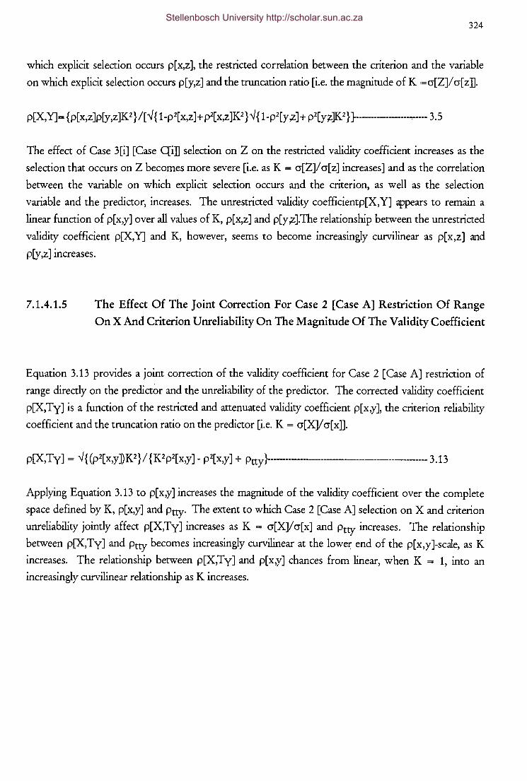
324
which explicit selection occurs p[x,z], the restricted correlation between the criterion and the variable
on which explicit selection occurs p[y,z] and the truncation ratio [i.e. the magnitude of K =cr[Z]/cr[z].
p[X,Y]= {p[x,z]p[y,z]K2 }/[--./{ 1-p2[x,z]+ p2[x,z]K2 }--./{ 1-p2[y ,z]+ p2[y~]K2 } }------~--- 3.5
The effect of Case 3[i] [Case qi] selection on Z on the restricted validity coefficient increases as the
selection that occurs on Z becomes more severe [i.e. as K = cr[Z]/ cr[ z] increases] and as the correlation
between the variable on which explicit selection occurs and the criterion, as well as the selection
variable and the predictor, increases. The unrestricted validity coefficientp[X, Y] appears to remain a
linear function of p[x,y] over all values of K, p[x,z] and p[y ,z].The relationship between the unrestricted
validity coefficient p[X,Y] and K, however, seems to become increasingly curvilinear as p[x,z] and
p[y,z] increases.
7.1.4.1.5 The Effect Of The Joint Correction For Case 2 [Case A] Restriction Of Range
On X And Criterion Unreliability On The Magnitude Of The Validity Coefficient
Equation 3.13 provides a joint correction of the validity coefficient for Case 2 [Case A] restriction of
range directly on the predictor and the unreliability of the predictor. The corrected validity coefficient
p[X,Ty] is a function of the restricted and attenuated validity coefficient p[x,y], the criterion reliability
coefficient and the truncation ratio on the predictor [i.e. K = cr[X]/ cr[x]].
p[X,Ty] = --./ { (p2[ x,y] K 2 } I { K 2 p2[ x,y] - p2[ x,y] + Ptty }--------------------------------------------- 3.13
Applying Equation 3.13 to p[x,y] increases the magnitude of the validity coefficient over the complete
space defined by K, p[x,y] and Ptty· The extent to which Case 2 [Case A] selection on X and criterion
unreliability jointly affect p[X,Ty] increases as K = cr[X]/cr[x] and Ptty increases. The relationship
between p[X,Ty] and Ptty becomes increasingly curvilinear at the lower end of the p[x,y]-scale, asK
increases. The relationship between p[X,Ty] and p[x,y] chances from linear, when K = 1, into an
increasingly curvilinear relationship as K increases.
Stellenbosch University http://scholar.sun.ac.za
7.1.4.2
7.1.4.2.1
325
The Effect Of Separate And Combined Statistical Corrections For Restriction Of
Range And Random Measurement Error On The Magnitude Of The Standard
Error Of The Pearson Correlation Coefficient
The Effect Of The Correction For Criterion Unreliability Only On The
Magnitude Of The Standard Error Of The Pearson Correlation Coefficient
Equation 4.22 provides the expression for the square of the standard error of the partially disattenuated
validity coefficient derived by Kelly [1947, p. 529] cr2[p~[X,Ty ]]is dependent on the attenuated validity
coefficient p[X,Y], the split-half reliability coefficient p'ttY and the number of cases included in the
validation group.
cr2[p ~[X,Ty ]] = p2[X,Ty ]/ (n-2)(p2[X,Ty ]+ p-I[X,Y]-p '-!tty+ 4p'-2tty-5/ 4)------------------------ 4.22
The standard error of the partially disattenuated validity coefficient decreases curvilinearly as the
reliability of the criterion increases, increases sharply as the attenuated correlation increases at the lower
end of the criterion reliability scale but decreases slowly as the attenuated co~relation increases at the
upper end of the criterion reliability scale. The standard error of the partially disattenuated validity
coefficient furthermore decreases as the sample size increases.
The standard error of the partially disattenuated validity coefficient is greater than the standard error of
the attenuated validity coefficient in the whole space defined by p[X, Y] and Ptt y, ex:cept for a small
region characterised by high p[X,Y] and PttY values. This region in which the standard error of the
partially disattenuated validity coefficient decreases relative to the standard error of the attenuated
validity coefficient gradually seems to expands to lower p[X, Y] values as n increases. This finding
might, however, be attributable to the known weakness of the expression [Equation 4.13] used to
represent the standard error of the attenuated validity coefficient in the analysis towards the upper end
of the p[X,Y] scale.
Equations 4.23 - 4.25 provide three alternative expressions of the standard error of the partially
disattenuated validity coefficient derived by Bobko and Rieck [1980, p. 388].
cr2[p ~[X, T y ]] = [A+ B-C] ------------------------------------------------------------------------------------- 4.23
cr2[p ~ [X, T y ]] = [A+ B ]---------------------------------------------------------------------------------------------- 4.2 4
Stellenbosch University http://scholar.sun.ac.za
326
cr2[p A[X,Ty ]] = [A]------------------------------- -------------- 4.25
Where:
The conditions under which each expression becomes appropriate were described earlier.
The standard error of the partially disattenuated validity coefficient calculated through Equations 4.23
and 4.24 tends to increase curvilinearly as the attenuated correlation increases at low values of Ptt y but
this trend gradually reverses as PttY increases, until, at the upper end of the criterion reliability scale, the
standard error moderately decreases as p[X,Y] increases. The standard error produced by Equations
4.23 and 4.24, furthermore, increase as the criterion reliability decreases, peaks at the maximum p[X,Y]
value possible, given Ptt y and decreases as sample size increases. The first two expressions derived by
Bobko and Rieck [1980] therefore tend to behave essentially in the same way as the expression derived
by Kelly [1947].
The standard error of the partially disattenuated validity coefficient calculated through Equation 4.25
also tends to increase as Ptt y decreases and also decreases as n increases. However, the standard error
obtained through Equation 4.25 reacts differently to an increase in the attenuated correlation.
Although still curvilinearly related to p[X,Y], the standard error now seems to gradually decrease as
p[X,Y] increases for all values of PttY.
For Equations 4.23, 4.24 and 4.25, the standard error of the partially disattenuated validity coefficient
exceeds the standard error of the attenuated validity coefficient for all permissible combinations of
values of p[X,Y], PttY and n. For the first two standard error expressions derived by Bobko and Rieck
[1980] the reaction of ratio of the standard errors of the partially disattenuated and attenuated validity
coefficients [V = cr[p A J/ cr[p A]] to changes in p[X,Y], Ptt y and n is very similar. The ratio V increases
as p[X,Y] increases and PttY decreases. The ratio V peaks both at high PttY and high p[X,Y] and at
low PttY combined with low-moderate p[X,Y].
For Equation 4.25, however, V remains constant over changes in p[X,Y] for all values of PttY and
increases as Ptt y decreases. This would imply that the standard error of the attenuated validity
coefficient shadows/tails the standard error of the partially disattenuated validity coefficient over all
Stellenbosch University http://scholar.sun.ac.za
327
values of p[X,Y] and PttY• but that the latter tend to gain on the former as the criterion reliability
decreases.
7.1.4.2.2 The Effect Of The Correction For Case 1 [Case B] Restriction Of Range On The
Magnitude Of The Standard Error Of The Pearson Correlation Coefficient
No formal derivation of a specific expression for the standard error of the correlation coefficient
corrected for Case 1 [Case B] selection could be uncovered. The reaction of the standard error of the
correlation coefficient to Case 1 [Case B] selection was therefore not examined.
7.1.4.2.3 The Effect Of The Correction For Case 2 [Case A] Restriction Of Range On The
Magnitude Of The Standard Error Of The Pearson Correlation Coefficient
Equation 4.35 provides the expression for the square of the standard error of the validity coefficient
corrected for Case 2 [Case A] restriction of range on X derived by Bobko and Rieck [1980, p. 390]:
cr2[p A[X,Y]] = {K 2(1-p2[x,y ]+ p2[x,y ]K2)-3} { (1-p2[x,y ])2 In}------------------------------------------------ 4.35
Where: K = ( cr[X]/ cr[ x ])
The standard error of the validity coefficient corrected for Case 2 [Case A] restriction of range seems to
increase as the restricted validity coefficient decreases and to increase relatively sharply as K increases at
low values of p[x,y], but to decrease slowly as K increases at high values of p[x,y]. At would be
expected, the standard error increases as n decreases.
The ratio of the standard error of the validity coefficient corrected for Case 2 [Case A] restriction of
range to the standard error of the observed, restricted validity coefficient [i.e. V = cr[p A cJ/ cr[p A]] seems
to copy/imitate the behaviour of the standard error of the corrected coefficient as described above.
The standard error of the validity coefficient corrected for Case 2 [Case A] restriction of range generally
is greater than the standard error of the observed, uncorrected validity coefficient. However, V does
decrease below unity in a relatively small region of the p[x,y],K plane characterised by high p[x,y] and
K values. When estimating cr[p A] through Equation 4.13, cr[p A cJ estimated through Equation 4.35 will
thus exceed the former at small selection ratios and high restricted [i.e. uncorrected] correlations.
Stellenbosch University http://scholar.sun.ac.za
328
7.1.4.2.4 The Effect Of The Correction For Case C Restriction Of Range On The
Magnitude Of The Standard Error Of The Pearson Correlation Coefficient
Equation 4.36 provides the expression for the standard error of the validity coefficient corrected for
Case 3[i] [Case C[i]] restriction of range derived by Allen and Dunbar [1990, p. 80] .
..J cr2[p A [X,Y]] = { p2'[X,Y]cr2[p A [x,y ]+ p2'[X,Z]cr2[p A [ x,z ]]+ p2 '[Y ,Z]cr2[p A [y ,z ]]+
2p'[X,Y]p'[X,Z]cr[p A[x,y],p A[x,z]] +2p'[X;Y]p'[Y ,l]cr[p A[x,y],p A[y,z]] +
2 p '[X,Z] p '[Y,Z]cr[p A [ x,z ], p A [y,z]]} lh --------------------------------------- 4. 3 6
Where:
p'[X,Y] indicates the partial derivative of the adjusted correlation p[X,Y] with respect to the unadjusted
correlation p[ x,y ]; specifically
p'[X,Y] = (1+ Wp2[x,z])-lh(1+ Wp2[y,z])-lh
p'[X,Z] = W(1 + W p2[x,z])-312(1 + W p2[y,z])-lh (p[y,z]-p[x,y]p[x,z])
p'[Y,Z] = W(1 + W p2[x,z])-lh (1 + W p2[y,z])-312(p[x,z]-p[x,y]p[y ,z]; and
W = ( cr2[Z]/ cr2[ z ]) -1
The two large sample estimates of the sampling variance of a correlation corrected for indirect [Case
3[i] [Case C[i]]] selection proposed by Allen and Dunbar [1990] differ in terms of the equations chosen
for the estimation of the asymptotic variance and covariance components. The difference
fundamentally lies in the assumptions on which these estimates are based. Allen and Dunbar [1990, p.
86] distinguish between two sets of assumptions, namely:
);> set A; "error In to second and third powers is negligible, linearity of regression, and
mesokurtosis of the joint distribution of explicit and implicit variables; and
);> set B; error/n to second and third powers is negligible and linearity of regression."
Only the variance and covariance equations based on the more stringent assumption set A are
presented below.
cr[p A[x,y],pA[x,z]] = (1/n){p[y,z](1-p2[x,z]-p2[x,y]-112p[x,y]p[x,z](1-p2[y ,z}p2[x,y ]
p2[x,z])}
Stellenbosch University http://scholar.sun.ac.za
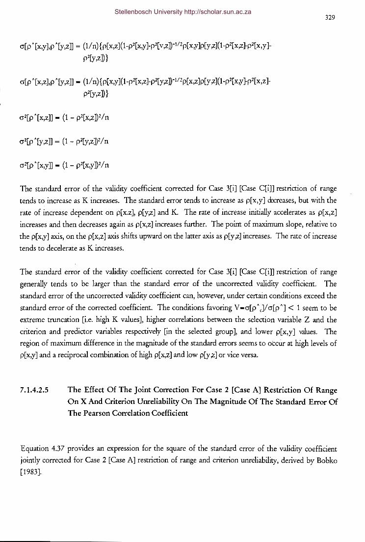
cr[p "[x,y],p "[y,z]] = (1/ n){p[x,z ](1-p2[x,y]-p2[ v,z])-112p[x,y]p[y ,z](1-p2[x,z]-p2[x,y ]
p2[y,z]}
cr[p "[x,z],p "[y,z]] = (1/ n){p[x,y](1-p2[x,z]-p2[y,z]-112p[x,z]p[y ,z](1-p2[x,y]-p2[x,z]
p2[y,z]}
329
The standard error of the validity coefficient corrected for Case 3[i] [Case C[i]] restriction of range
tends to increase as K increases. The standard error tends to increase as p[x,y] ckreases, but with the
rate of increase dependent on p[x.z], p[y,z] and K. The rate of increase initially accelerates as p[x,z]
increases and then decreases again as p[x,z] increases further. The point of maximum slope, relative to
the p[x,y] axis, on the p[x,z] axis shifts upward on the latter axis as p[y ,z] increases. The rate of increase
tends to decelerate as K increases.
The standard error of the validity coefficient corrected for Case 3[i] [Case C[i]] restriction of range
generally tends to be larger than the standard error of the uncorrected validity coefficient. The
standard error of the uncorrected validity coefficient can, however, under certain conditions exceed the
standard error of the corrected coefficient. The conditions favoring V = cr[p "J/ cr[p "] < 1 seem to be
extreme truncation [i.e. high K values], higher correlations between the selection variable Z and the
criterion and predictor variables respectively [in the selected group], and lower p[ x, y] v.llues. The
region of maximum difference in the magnitude of the standard errors seems to occur at high levels of
p[x,y] and a reciprocal combination of high p[x,z] and low p[y ,z] or vice versa.
7.1.4.2.5 The Effect Of The Joint Correction For Case 2 [Case A] Restriction Of Range
On X And Criterion Unreliability On The Magnitude Of The Standard Error Of
The Pearson Correlation Coefficient
Equation 4.37 provides an expression for the square of the standard error of the validity coefficient
jointly corrected for Case 2 [Case A] restriction of range and criterion unreliability, derived by Bobko
[1983].
Stellenbosch University http://scholar.sun.ac.za
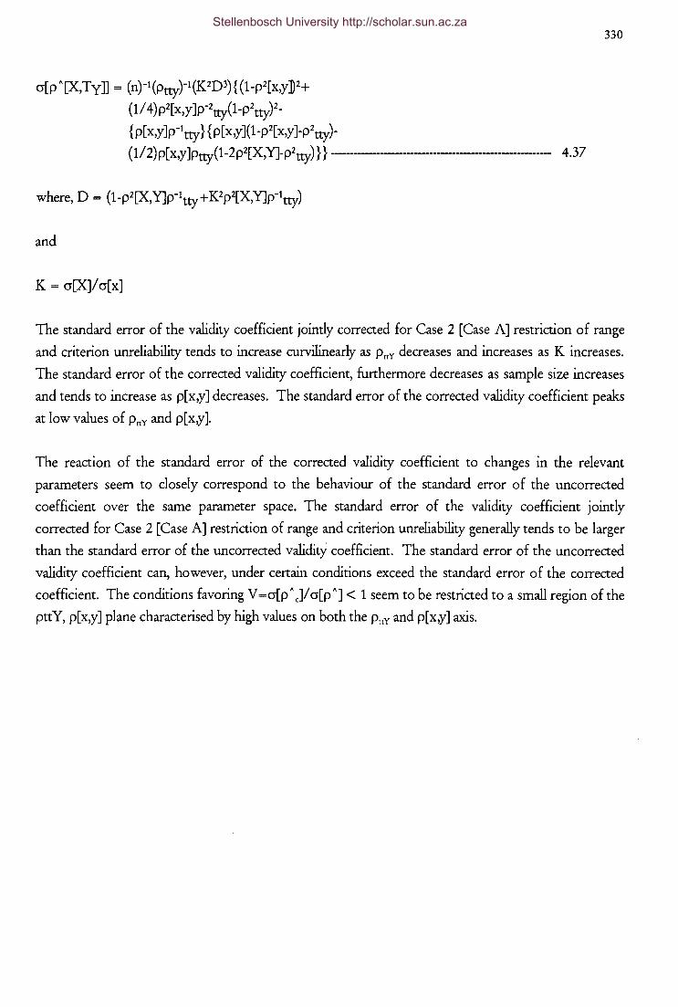
cr[pA[X,Ty]] = (n)-1(ptty)-1(K2D3){(1-p2[x,y]2+
(1/ 4) p2[ x,y ]p-2tty(1-p2tty)2-
{p[ x,y]p-1ny} {p[x,y](1-p2[x,y ]-p2ny)-
(1/2)p[x,y]pny(1-2p2[X,Y]-p2ny)}} ------------------------------ 4.37
and
K = cr[X]/ cr[ x]
330
The standard error of the validity coefficient jointly corrected for Case 2 [Case A] restriction of range
and criterion unreliability tends to increase curvilinearly as PnY decreases and increases as K increases.
The standard error of the corrected validity coefficient, furthermore decreases as sample size increases
and tends to increase as p[ x,y] decreases. The standard error of the corrected validity coefficient peaks
at low values of PnY and p[x,y].
The reaction of the standard error of the corrected validity coefficient to changes in the relevant
parameters seem to closely correspond to the behaviour of the standard error of the uncorrected
coefficient over the same parameter space. The standard error of the validity coefficient jointly
corrected for Case 2 [Case A] restriction of range and criterion unreliability generally tends to be larger
than the standard error of the uncorrected validio/ coefficient. The standard error of the uncorrected
validity coefficient can, however, under certain conditions exceed the standard error of the corrected
coefficient. The conditions favoring V=cr[pA cJ/cr[pA] < 1 seem to be restricted to a small region of the
pttY, p[x,y] plane characterised by high values on both the PnY and p[x,y] axis.
Stellenbosch University http://scholar.sun.ac.za
7.1.4.3
7.1.4.3.1
331
The Effect Of Separate And Combined Statistical Corrections For Restriction Of
Range And Random Measurement Error On The Magnitude Of The
Empirically Derived Exceedence Probability aB
The Effect Of The Correction For Criterion Unreliability Only On The
Magnitude Of The Empirically Derived Exceedence Probability
The Bobko and Rieck [1980] expressions for the standard error of the partially disattenuated validity
coefficient were used to assess the impact of the correction for criterion unreliability on the empirically
derived exceedence probability.
7.1.4.3.1.1 The Reliability Coefficient Given A Priori By Theoretical Assumption Or
Previously Accepted Knowledge
The empirically derived exceedence probability ab is not affected by the correction for criterion
unreliability. The conditional probability of observing the corrected validity coefficient under Ho is the
same as the conditional probability of observing the uncorrected validity coefficient under Ho. The
statistical significance tests for the uncorrected and corrected validity tests are asymptotically identical if
Ptt y is known a priori.
7.1.4.3.1.2 The Reliability Coefficient Obtained From An Independent Data Set
If the reliability coefficient used to correct the validity coefficient for the unreliability of the criterion is
obtained from an independent data set, and the appropriate expression for the standard error is
subsequently used, the empirical exceedence probability is affected. The probability of observing the
corrected correlation in a sample of size n drawn from a population where the two variables being
correlated are, in fact, independent is consistently larger than the conditional probability of observing
the attenuated coefficient in a sample of the same size under HQ.
The increase in ab produced by the partial correction for attenuation has the effect of changing some
significant correlations into insignificant partially disattenuated correlations. The change in decision
Stellenbosch University http://scholar.sun.ac.za
332
occurs in a specific region of the p[X,Y] axis as a function of sample size. The region shifts lower
down on the p[X,Y] axis as sample size increases.
7.1.4.3.1.3 The Reliability Coefficient Obtained From The Same Data Set
If the reliability coefficient used to correct the validity coefficient for the unreliability of the criterion is
obtained from the same data set, and the appropriate expression for the standard error is subsequently
used, the empirical exceedence probability is affected. . The probability of observing the corrected
correlation in a sample of size n drawn from a population where the two variables being correlated are,
. in fact, independent is consistently larger than the conditional probability of observing the attenuated
coefficient in a sample of the same size under Ho. The nature of the effect is very similar to those
found for the Bobko and Rieck [1980] Case II expression as described in the previous paragraph.
The increase in ab produced by the partial correction for attenuation has the effect of changing some
significant correlations into insignificant partially disattenuated correlations. The change in decision
occurs in a specific region of the p[X,Y] axis as a function of sample size. The region shifts lower
down on the p[X,Y] axis as sample size increases.
7.1.4.3.2 The Effect Of The Correction For Case 1 [Case B] Restriction Of Range On The
Magnitude Of The Empirically Derived Exceedence Probability
No formal derivation of a specific expression for the standard error of the correlation coefficient
corrected for Case 1 [Case B] selection could be uncovered. The effect of the correction for Case 1
[Case B] restriction of range on the magnitude of the empirically derived exceedence probability could,
therefore, not be examined.
7.1.4.3.3 The Effect Of The Correction For Case 2 [Case A] Restriction Of Range On The
Magnitude Of The Empirically Derived Exceedence Probability
The conditional probability of observing the corrected validity coefficient under Ho equals the
conditional probability of observing the uncorrected validity coefficient under Ho wren K = cr[X]/ cr[x]
= 1. This is a logically necessary result, since pA[x,y] = pA[X,Y] and cr[pA[x,y]] = cr[pA[X,Y]]when K =
Stellenbosch University http://scholar.sun.ac.za
333
1. For all possible combinations of n, pA[x,y] and K>l, the probability of observing the corrected
validity coefficient under Ho is consistently smaller than the probability of observing the corresponding
uncorrected validity coefficient value under Ho. The effect of the correction for Case 2 [Case A]
restriction of range on ab intensifies curvilinearly as the uncorrected sample correlation pA[x,y] and K
mcreases.
The decrease in the conditional probability ab has the effect of changing some insignificant
uncorrected correlations into significant corrected correlations. This effect seems to be relatively
sensitive to sample size. At n ~ 120 Case 2 [Case A] restriction of range corrections to the validity
coefficient no longer has the effect of changing the significance test outcome [given a significance level
of 0.05 and a one-tailed test]. The change in decision occur in a specific, restricted region in the
p A [ x,y ], K space as a function of sample size n. as sample size increases, the region shifts to lower
values of p A [ x,y ], but simultaneously also higher values of K.
7.1.4.3.4 The Effect Of The Correction For Case 3[i] [Case C[i]] Restriction Of Range On
The Magnitude Of The Empirically Derived Exceedence Probability
Correcting the validity coefficient for Case 3[i] [Case C[i]] restriction of range produces either a
decrease or an increase in the conditional probability of observing the corrected validity coefficient
under Ho: p[X,Y] = 0 relative to the conditional probability of observing the uncorrected validity
coefficient under Ho: p[x,y] = 0. These changes in ab brought about by the correction for restriction
of range has the effect of changing some insignificant uncorrected correlations into significant
corrected correlations and vice versa.
The region in which correlations change from insignificant to significant seem to occur at the lower end
of the pA[x,y] axis for moderate to high pA[x,z] values. This region seems to shift towards zero on the
p A[x,y] axis asK increases. The region in which the decision on significance of the validity coefficient is
affected, shrinks as n increases.
The region in which correlations change from significant to insignificant seem to occur at the lower end
of the pA[x,y] axis for moderate to high pA[x,y] values. This region seems to shift towards the upper
end of the pA[x,y] axis as pA[y,z] increases and to spread towards zero on the pA[x,z] axis as K
decreases. The region in which the decision on significance of the validity coefficient is affected,
shrinks as n increases.
Stellenbosch University http://scholar.sun.ac.za
334
The conditional probability of observing the corrected validity coefficient under Ho: p[X,Y] =0 seems
to decrease relative to the conditional probability of observing the uncorrected validity coefficient
under Ho: p[x,y] = 0 as K increases, as the correlation of the predictor with the selection variable Z
increases, as the correlation of the criterion with the predictor increases and as p "[x,y] decreases.
7.1.4.3.5 The Effect Of The Joint Correction For Case 2 [Case A] Restriction Of Range
On X And Criterion Unreliability On The Magnitude Of The Empirically
Derived Exceedence Probability
For all combinations of n, p"[x,y], PnY and K > 1, the probability of observing the uncorrected validity
coefficient in a sample of size n, conditional on HQ: p[x,y] = 0, is consistently bigger than the
probability of observing the corresponding double corrected validity coefficient, conditional on the
hypothesis that p[X,Ty] = 0. This effect of the joint correction for Case 2 [Case A] restriction of
range and criterion unreliability on ab intensifies as p" [x,y] and K increases and PaY decreases.
The decrease in ab, produced by the joint correction, has the effect of changing some insignificant
uncorrected correlations into significant corrected correlations when K > 1. This effect seems to be
fairly sensitive to sample size. At n 2:: 120, double corrections to the validity coefficient no longer has
the effect of changing the hypothesis test outcome.
The change in the hypothesis test outcome seems to occur in the lower region of the p "[x,y] axis and
the full range of PnY values as a function of K and sample size n. As sample size increases, the region
shifts to lower values of p " [ x,y] and also seems to become more restricted to the lower region of the
PrrY ax.ts.
Stellenbosch University http://scholar.sun.ac.za
7.1.4.4
7.1.4.4.1
7 .1.4.4.1.1
335
The Effect Of Separate And Combined Statistical Corrections For Restriction Of
Range And Random Measurement Error On The Magnitude Of The A Priori
Probability Of Rejecting Ho If Ho Is False
The Effect Of The Correction For Criterion Unreliability Only On The
Magnitude Of The A Priori Probability Of Rejecting Ho If Ho Is False
The Reliability Coefficient Given A Priori By Theoretical Assumption Or
Previously Accepted Knowledge
The power of the statistical significance test of the validity coefficient will not be affected by the
correction for criterion unreliability if the standard error of the corrected validity coefficient is
calculated by the Bobko and Rieck [1980] Case III expression.
7.1.4.4.1.2 The Reliability Coefficient Obtained From An Independent Sample
The power of the statistical significance test of the corrected validity coefficient is negatively affected
[i.e. the power decreases] if the standard error of the corrected validity coefficient is calculated by the
Bobko and Rieck [1980] Case II expression.
7.1.4.4.1.3 The Reliability Coefficient Obtained From The Same Sample
The power of the statistical significance test of the corrected validity coefficient is negatively affected
[i.e. the power decreases] if the standard error of the corrected validity coefficient is calculated by the
Bobko and Rieck [1980] Case I expression. The negative effect of Case I partial corrections for
attenuation on statistical power increases curvilinearly with increases in the effect size assumed for the
uncorrected validity coefficient over all levels of criterion reliability.
Stellenbosch University http://scholar.sun.ac.za
7.1.4.4.2
336
The Effect Of The Correction For Case 1 [Case B] Restriction Of Range On The
Magnitude Of The A Priori Probability Of Rejecting Ho If Ho Is False
No formal derivation of a specific expression for the standard error of the correlation coefficient
corrected for Case 1 [Case B] selection could be uncovered. The effect of the correction for Case 1
[Case B] restriction of range on the magnitude of the a priori probability of rejecting the null hypothesis
conditional on the null hypothesis being false, could therefore not be examined.
7.1.4.4.3 The Effect Of The Correction For Case 2 [Case A] Restriction Of Range On The
Magnitude Of The A Priori Probability Of Rejecting Ho If Ho Is False
The statistical power of the statistical significance test of the validity coefficient increases if the
correction for Case 2 [Case A] restriction of range is applied to the observed, restricted correlation
coefficient and the uncorrected effect size estimate.
7.1.4.4.4 The Effect Of The Correction For Case 3[i] [Case C[i]] Restriction Of Range On
The Magnitude Of The A Priori Probability Of Rejecting Ho If Ho Is False
Case 3[i] [Case C[i]] corrections for restriction of range effect statistical power both positively and
negatively, depending on the applicable parameter settings. Case 3[i] [Case C[i]] seem to have
maximum adverse impact on statistical power when pA[x,y] is high and pA[x,z] and pA[y,z] is low. K
seem to affect power by aggravating the effect of the aforementioned parameters as K increases.
Corrections for Case 3[i] [Case Qi] restriction of range seem to have maximum beneficial impact on
statistical power under those conditions where Case C restrictions have their greatest impact, namely
when pA[x,y] is low and pA[x,z] and pA[y,z] is high. K again seems to affect power by enhancing the
effect of the aforementioned parameters as K increases.
Stellenbosch University http://scholar.sun.ac.za
7.1.4.4.5
337
The Effect Of The Joint Correction For Case 2 [Case A] Restriction Of Range
On X And Criterion Unreliability On The Magnitude Of The A Priori Probability
Of Rejecting Ho If Ho Is False
The statistical power of the significance test of the validity coefficient is improved by the double
correction for restriction of range and criterion unreliability, provided the uncorrected effect size
estimate is also corrected via the appropriate formula to obtain the corrected effect size estimate.
Maximum power benefits are obtained by the double correction when the initial uncorrected effect size
estimate is high, PnY is low and K is high. Although n affects power, it does not seem to affect the
change in power brought about by the double correction to the correlation coefficient.
7.1.4.5
7.1.4.5.1
The Effect Of Separate And Combined Statistical Corrections For Restriction Of
Range And Random Measurement Error On The Magnitude Of The Intercept
And Slope Parameters Of The Regression Of The Criterion On The Predictor
The Effect Of The Correction For Criterion Unreliability Only On The
Magnitude Of The Intercept And Slope Parameters Of The Regression Of The
Criterion On The Predictor
The regression of the criterion on the predictor remains unaffected by the partial correction for the
attenuating effect of the unreliability of the criterion. Neither theY-axis intercept, nor the X-axis slope
are affected by the removal of random measurement error from the criterion.
The expected criterion performance conditional on X will therefore remain unaffected. The decision
on applicant will therefore not change due to the partial correction for attenuation, irrespective of
whether selection is restricted by quotas or not.
Stellenbosch University http://scholar.sun.ac.za
338
7.1.4.5.2 The Effect Of The Correction For Case 1 [Case B] Restriction Of Range On The
Magnitude Of The Intercept And Slope Parameters Of The Regression Of The
Criterion On The Predictor
If selection occurs directly on the predictor X, but the restricted and unrestricted variances are known
only for the criterion Y, then by assumption neither the regression of Y on X nor the criterion variance
conditional on X will be affected. Thus, by assumption Equations 6.22 and 6.23 apply. The same
notation convention as before is used.
p[Y I X]= p[X,Y](cr[Y]/cr[X])
= p[x,y](cr[y]/cr[x])
= p[y I X] ----------------------------------------------------------------------------------------------------- 6. 22
cr2[Y I X] = cr2[Y](1 - p2[X,Y])
= cr2[y](1 - p2[x,y]
= p[y I x] ------------------------------------------------------------------------------------------ 6.23
Since Equation 6.22 reflects the assumption that !-l[Y I Xi] is not altered by explicit selection on X,
Equation 6.24 also applies.
a[Y I X] = 1-l[Y] - P[Y I X]!-l[X]
= !-l[y]- P[y I x]!-l[x]
= a[y I x] ---------------------------------------------------------------------------------------------- 6.2 4
Although the magnitude of the correlation is influenced by Case 1 [Case B] selection on X, and
although the standard errors of the regression coefficients will increase due to this type of Case 1 [Case
B] selection, the relevant decision function [and therefore also the contents of the strategy matrix] will
not be affected by Case 1 [Case B] selection on X. Corrections to the parameters of the decision
function to compensate for this type of Case 1 [Case B] restriction of range are consequently not
required.
If , however, the selection occurs directly on the criterion, but the restricted and unrestricted variances
are known only for the predictor, then the regression of Y on X is affected. Equations 6.25 and 6.26
demonstrate that corrections of the parameters of the regression of Y on X for the effect of Case 1
[Case B] selection on Y produce an increase in the slope parameter and a decrease in the intercept.
p[Y I X] = p[y I x] { ( 11 p2[x,y ]) - (K 2 I p2[x,y] ( 1-p[ x,y ]) } ------------------------------------------------- 6.25
Stellenbosch University http://scholar.sun.ac.za
339
a[Y I X] = f.L[Y] - P[Y I X]f.l[X]
= (p[x,y]cr[x]/cr[y]-1(fl[X]- f.L[x]) + fl[y]- P[Y I X]f.l[XJ-------------------------- 6.26
The expression for the regression of Y on X, corrected for Case 1 [Case B] selection on Y, is shown as
Equation 6.27.
E[Y IXJ = (p[x,y]cr[x]/cr[y]-1(f.l[X]- J.t[x]) + J.t(y] + {cr[y]/(p[x,y]cr[x]-
( cr[ x ]cr[y] I (p[ x,y ]cr2[X] ( 1 - p2[ x,y]} (Xi - J.t[X]}------------------------- 6.27
The change in the regression parameters implies that the regression equation derived from the selected
applicant group and the regression equation that would have been obtained from the unrestricted
applicant group will intersect at some point Xs on the X-axis. Consequently, for all Xi < Xs E[y I Xi]
will overestimate E[Y I Xi] while for all Xi > Xs E[y I Xi] will underestimate E[Y I Xi]. Correcting the
parameters of the decision function for Case 1 [Case B] selection on Y, consequently will have the
effect of elevating the expected criterion performance for all Xi > Xs, while depressing it for all Xi < Xs.
The correction of the decision function for Case 1 [Case B] selection on Y will not affect the applicants
selected if selection is restricted by quotas and strict top down selection applies. Although E[Y I Xi] :t:
E[y I Xi], if E[y I Xi] > E[y I Xj] then E[Y I Xi] > E[Y I Xj]. The same Nv applicants would therefore still be
selected.
In the case of selection unrestricted by quotas, however, the use of the corrected decision function will
affect the selection decision-making. The nature of the effect will depend on the position of Xc
[derived from Y c via the decision function calculated on the selected applicant group] relative to Xs . If Xs < Xc the number of applicants satisfying the entry requirement [i.e. E[Y I Xi] > Y cJ will increase. If Xs > Xc [unlikely since it would imply a very low Y con a positive criterion], the number of applicants
qualifying for selection will decrease.
7.1.4.5.3 The Effect Of The Correction For Case 2 [Case A] Restriction Of Range On The
Magnitude Of The Intercept And Slope Parameters Of The Regression Of The
Criterion On The Predictor
If Case 2 [Case A] selection occurs directly on the predictor X, then by assumption, neither the
regression of Y on X nor the criterion variance conditional on X will be affected. No corrections to
the parameters of t he regression equation or the standard error of estimate are therefore required. The
Stellenbosch University http://scholar.sun.ac.za
340
regression of X on Y would be affected, but since it is of no real interest in selection validation
research, no justification seems to exist to explore it further.
If Case 2 [Case A] selection occurs directly on the criterion Y, then by assumption, neither the
regression of X on Y nor the predictor variance conditional on Y will be affected. The regression of Y
on X and the criterion variance conditional on X would be affected. The probability of Case 2 [Case A]
selection on Y actually occurring in the context of selection validation research, however, seems for all
practical purposes to be zero. Although appropriate correction formula therefore should exist, there
once more seems to be no practical justification to try and uncover their formulation.
7.1.4.5.4 The Effect Of The Correction For Case 3[i] [Case C[i]] Restriction Of Range On
The Magnitude Of The Intercept And Slope Parameters Of The Regression Of
The Criterion On The Predictor
Equation 6.29 provides an expression for the slope of the regression of Y on X for the unselected
population. Equation 6.29 assumes Case 3[i] [Case C[i]] selection on Z.
P[YIXJ = {(p[x,y]-p[x,z]p[y,z]) + (p[x,z]p[y,z]K2)}/{(1- p[x,z] + p2[ x,z ]K 2)} ( cr[y ]/ cr[ x ])------------------------------------------------------------------------------------- 6.29
Equation 6.30 provides an expression for the intercept of the regression of Y on X for the unselected
population derived from a[ylxJ and Case 3[i] [Case C[i]]selection.
a[Y I X] = { J.![y] + p[y,z ]( cr[y ]/ cr[ z ]) (Jl[Z] - Jl[ z ]) } -
p[Y I X]{J.![x] + p[x,z](cr[x]/ cr[z])(Jl[Z] - Jl[z]) }------------------------------------------------ 6.30
Equations 6.29 and 6.30 generally have the effect of increasing the slope of the regression of Y on X
relative to the slope of the regression of y on x and, concomitantly, decreasing the intercept. There are,
however, parameter settings were the opposite effect is achieved.
The regression of y on x and the estimated/ corrected regression of Y on X will intersect at some point
Xs on the X -axis. The magnitude and direction of the change in the expected criterion performance
associated with applicants attributable to the application of Equations 6.29 and 6.30 will depend on the
position of Xi relative to Xs and the magnitude of p[YIXJ relative to p[ylxJ. TABLE 6.1 presents a
summary of the effect of Equations 6.29 and 6.30 on the expected criterion performance associated
with applicants.
Stellenbosch University http://scholar.sun.ac.za
341
Correction for Case 3[i] [Case Qi] selection on Z will [probably] not affect selection decision-making
based on expected criterion performance when selection quotas limit the number of applicants
required. The same N s applicants will thus still be selected as long as the principle of strict top down
selection is adhered to.
In the case of unrestricted selection, however, corrections for Case C selection on Z probably would
affect selection decision-making. Since Y c is assumed constant, the change in the expected criterion
performance attributable to Equations 6.29 and 6.30 would probably move a number of applicants
across the critical criterion cutoff. The direction of the migration would once more depend on the
position of Xi relative to Xs and the magnitude of p[Y IX] relative to p[y lx]. TABLE 6.2 presents a
summary of the anticipated effect of Equations 6.29 and 6.30 on the number of applicants fulfilling the
entty requirement for selection [i.e. E[Y I X] ~ Y c].
7.1.4.5.5 The Effect Of The Joint Correction For Case 2 [Case A] Restriction Of Range
On X And Criterion Unreliability On The Magnitude Of The Intercept And
Slope Parameters Of The Regression Of The Criterion On The Predictor
Equation 6.32 depicts the effect of the joint correction for Case 2 [Case A] selection on X and criterion
unreliability on the slope parameter of the regression of Ty on X.
p[Ty IX]= (p[X,Y]){ (p[x,y]cr[y]cr[X])/(cr[x]p[X,Y]) }(1/cr[X])
= p[x,y](cr[y]/cr[x])
= p[y I X]---------------------------------------------------------------------------------------------------- 6. 3 2
Equation 6.32 indicates that the slope parameter is not affected by the joint correction for Case 2 [Case
A] selection on X and criterion unreliability.
Equation 6.33 depicts the effect of the joint correction for Case 2 [Case A] selection on X and criterion
unreliability on the intercept parameter of the regression of Ty on X.
a[Ty I X] = )l[Y] - p[Y I X])l[X]
= a[y I x] ------------------------------------------------------------------------------------------------ 6. 3 3
The intercept parameter is therefore also not affected by the joint correction for Case 2 [Case A]
selection on X and criterion unreliability.
Stellenbosch University http://scholar.sun.ac.za
342
Equations 6.32 and 6.33 imply that the expected criterion performance associated with applicants will
not be affected by the simultaneous removal of random measurement error from the criterion and the
reversal of explicit selection on the predictor. Selection decision-making will consequently not be
affected by the simultaneous removal of random measurement error from the criterion and the reversal
of explicit selection on the predictor, irrespective of whether selection quotas apply or not.
7.1.4.6
7.1.4.6.1
The Effect Of Separate And Combined Statistical Corrections For Restriction Of
Range And Random Measurement Error On The Magnitude Of The Standard
Error Of Estimate Of The Regression Of The Criterion On The Predictor
The Effect Of The Correction For Criterion Unreliability Only On The
Magnitude Of The Standard Error Of Estimate Of The Regression Of The
Criterion On The Predictor
Equation 6.11 provides an expression for the square of the standard error of estimate, corrected for
criterion unreliability:
cr2[Ty I X] = cr2[Y][ptt y - p2[X,Y]]
:::;; cr2[Y I X] --------------------------------------------------------------------------------------------- 6.11
The effect of statistically removing random measurement error from the criterion is to reduce the
standard error of estimate.
The reduction in the standard error of estimate will, assuming a constant critical criterion cutoff Y 0
have the effect of moving Y c to a more extreme position in the conditional criterion distribution.
Consequently, for all Xi > Xc = [Y c - a]/~' P[Ty ?.. Y c I X= Xi] will increase relative to P[Y > Y c I x =
Xi]. Conversely, for all Xi < Xc = [Y c - a]/~, P[Ty ?.. Y c I X= Xi] will decrease relative to P[Y > Y c I x
= XiJ. For Xi = Xc the conditional probability will remain unaffected.
Partially correcting the standard error of estimate for the attenuating effect of criterion unreliability will,
however, very unlikely change the selection decisions on applicants when selection is restricted by
quotas. Although the conditional probabilities are altered by the correction, the rank-order of the
applicants in terms of their chances of success remain exactly the same. Consequently, the same top
Nv would still be selected. Partially correcting the standard error of estimate for the attenuating effect
Stellenbosch University http://scholar.sun.ac.za
343
of criterion unreliability will only affect restricted selection if an insufficient number of applicants
initially [i.e. prior to corrections] meet the entry requirement as.
In the case of unrestricted selection, however, partially correcting the standard error for criterion
unreliability could affect the selection decision on applicants by increasing the number of applicants
qualifying for selection [assuming as > 0.50]. Correcting the standard error for criterion unreliability
has the effect of pushing any conditional probability greater than 0.50 but less than as [assuming as > 0.50] towards, and possibly past, as, thus increasing the selection ratio. Correcting the standard error
for criterion unreliability has the effect of pushing the critical predictor cutoff corresponding to the
critical probability as towards the point Xc [as defined above] in the predictor distribution. The
selection ratio is consequently increased for any as > 0.50 and decreased for any as < 0.50
7.1.4.6.2 The Effect Of The Correction For Case 1 [Case B] Restriction Of Range On The
Magnitude Of The Standard Error Of Estimate Of The Regression Of The
Criterion On The Predictor
Case 1 [Case B] selection on X does not affect the standard error of estimate cr[Y I X]. Case 1 [Case B]
selection on Y, however, does affect the standard error of estimate cr[Y IX]. Equation 6.28 provides a
correction to the standard error of estimate cr[ylxJ for Case 1 [Case B] selection on Y.
cr2[Y I X] = cr[y ]{ { (1-p2[x,y] }{ 1 - (K2(1-p2[x,y ] 2)/ p2[x,y]} }------------------------------------------- 6.28
~ cr2[ylxJ
Correcting cr[y I x] for Case 1 [Case B] selection on Y via Equation 6.28 returns a corrected value
cr[Y I X] greater than the obtained standard error of estimate. The difference between the corrected and
uncorrected standard errors of estimate seems to be negatively related to the observed correlation
p[x,y].
Correction for Case 1 [Case B] restriction of range on Y effect both the expected criterion performance
conditional on X and the standard error of estimate. The effect of the change in expected criterion
performance on the conditional probability tends to oppose the effect of the change in the standard
error of estimate. The change in the expected criterion performance exerts an upward pressure on the
conditional probability for all Xi > Xs and a downward pressure for all Xi < Xs· The change in the
standard error of estimate, in contrast, produces the opposite effect. The reaction of the conditional
probability of success to the aforementioned corrections for Case 1 [Case B] selection on Y,
Stellenbosch University http://scholar.sun.ac.za
344
consequently, depends on the which one of the two processes dominate. However, no single answer to
this question exists.
Two points on the X-axis [Xhi & X10 J are postulated, positioned in such a way on both sides of Xs,
that Z[Yc; E[ylx=Xhi]] = Z[Yci E[YIX=Xhi] and Z[Yci E[ylx=Xl0 ]] = Z[Yci E[YIX=Xl0 ]]. The
conditional probability of success associated with applicants falling on Xhi or X10 wruld therefore not
be affected by the preceding corrections for Case 1 [Case B] selection on Y. However, for all Xi > X}u,
and all Xi < X10 , the effect of the change in expected criterion performance would dominate.
Consequently the conditional probability of success associated with those applicants falling above Xhi
will increase [assuming Y c > J.L[Y]], while the conditional probability of success associated with those
applicants falling below Xlo will decrease. Furthermore, for those applicants located between these two
cutoff points [i.e. Xlo < Xi < Xhi], the effect of the change in the standard error of estimate should
dominate and consequently the conditional probability should increase.
The application of Equations 6.27 and 6.28 will [probably] not affect selection decision-making based
on the conditional probability of success, if such selection is restricted by selection quotas.
The application of Equations 6.27 and 6.28 will, however, affect unrestricted selection decision-making
based on the conditional probability of success. The selection ratio should increase since the critical
acceptance probability as is constant while the conditional probability of success associated with those
applicants falling above Xhi increases. The number of applicants qualifying for selection therefore
mcreases.
7.1.4.6.3 The Effect Of The Correction For Case 2 [Case A] Restriction Of Range On The
Magnitude Of The Standard Error Of Estimate Of The Regression Of The
Criterion On The Predictor
The effect of the correction for Case 2 [Case A] restriction of range on the magnitude of the standard
error of estimate of the regression of Y on X was not examined.
Stellenbosch University http://scholar.sun.ac.za
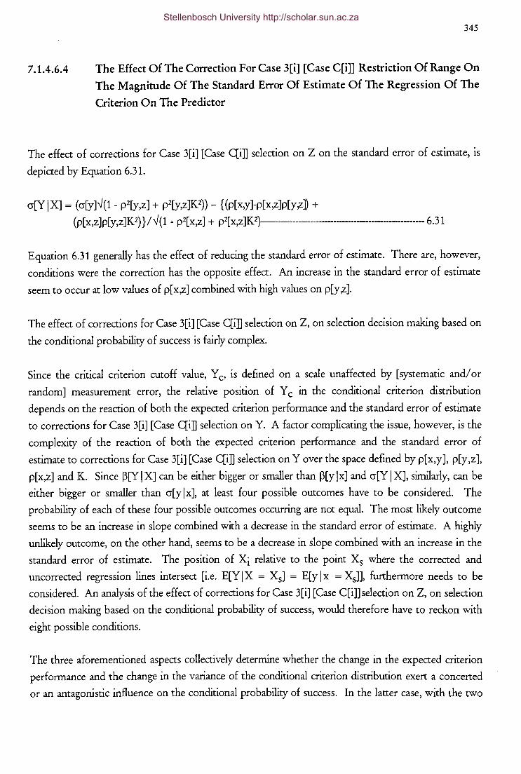
7.1.4.6.4
345
The Effect Of The Correction For Case 3[i] [Case C[i]] Restriction Of Range On
The Magnitude Of The Standard Error Of Estimate Of The Regression Of The
Criterion On The Predictor
The effect of corrections for Case 3[i] [Case Qi] selection on Z on the standard error of estimate, is
depicted by Equation 6.31.
cr[Y I X] = ( cr[y l'-' ( 1 - p2[y,z] + p2[y,z ]K 2)) - { (p[ x,y ]-p[ x,z ]p[y ,z] + (p[ x,z ]p[y,z ]K 2)} I'-' (1 - p2[ x,z] + p2[ x,z ]K 2)----------------------------------------------- 6.31
Equation 6.31 generally has the effect of reducing the standard error of estimate. There are, however,
conditions were the correction has the opposite effect. An increase in the standard error of estimate
seem to occur at low values of p[x,z] combined with high values on p[y ,z].
The effect of corrections for Case 3[i] [Case Qi] selection on Z, on selection decision making based on
the conditional probability of success is fairly complex.
Since the critical criterion cutoff value, Y 0 is defined on a scale unaffected by [systematic and/ or
random] measurement error, the relative position of Y c in the conditional criterion distribution
depends on the reaction of both the expected criterion performance and the standard error of estimate
to corrections for Case 3[i] [Case Qi] selection on Y. A factor complicating the issue, however, is the
complexity of the reaction of both the expected criterion performance and the standard error of
estimate to corrections for Case 3[i] [Case Qi] selection on Y over the space defined by p[x,y], p[y,z],
p[x,z] and K. Since p[Y I X] can be either bigger or smaller than p[y lxJ and cr[Y I X], similarly, can be
either bigger or smaller than cr[ylx], at least four possible outcomes have to be considered. The
probability of each of these four possible outcomes occurring are not equal. The most likely outcome
seems to be an increase in slope combined with a decrease in the standard error of estimate. A highly
unlikely outcome, on the other hand, seems to be a decrease in slope combined with an increase in the
standard error of estimate. The position of Xi relative to the point Xs where the corrected and
uncorrected regression lines intersect [i.e. E[Y I X = Xs] = E[y I x = XsJJ, furthermore needs to be
considered. An analysis of the effect of corrections for Case 3[i] [Case C[i]] selection on Z, on selection
decision making based on the conditional probability of success, would therefore have to reckon with
eight possible conditions.
The three aforementioned aspects collectively determine whether the change in the expected criterion
performance and the change in the variance of the conditional criterion distribution exert a concerted
or an antagonistic influence on the conditional probability of success. In the latter case, with the two
Stellenbosch University http://scholar.sun.ac.za
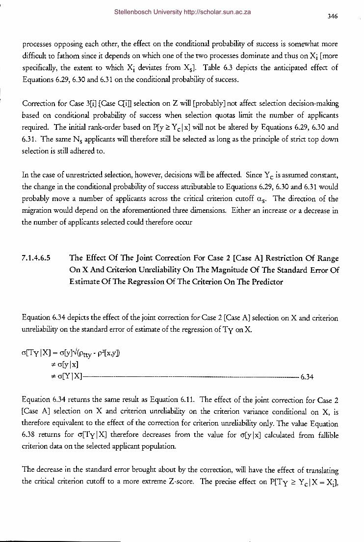
346
processes opposing each other, the effect on the conditional probability of success is somewhat more
difficult to fathom since it depends on which one of the two processes dominate and thus on Xi [more
specifically, the extent to which Xi deviates from XsJ. Table 6.3 depicts the anticipated effect of
Equations 6.29, 6.30 and 6.31 on the conditional probability of success.
Correction for Case 3[i] [Case qi] selection on Z will [probably] not affect selection decision-making
based on conditional probability of success when selection quotas limit the number of applicants
required. The initial rank-order based on P[y ~ Y c I x] will not be altered by Equations 6.29, 6.30 and
6.31. The same Ns applicants will therefore still be selected as long as the principle of strict top down
selection is still adhered to.
In the case of unrestricted selection, however, decisions will be affected. Since Y c is assumed constant,
the change in the conditional probability of success attributable to Equations 6.29, 6.30 and 6.31 would
probably move a number of applicants across the critical criterion cutoff as. The direction of the
migration would depend on the aforementioned three dimensions. Either an increase or a decrease in
the number of applicants selected could therefore occur
7.1.4.6.5 The Effect Of The Joint Correction For Case 2 [Case A] Restriction Of Range
On X And Criterion Unreliability On The Magnitude Of The Standard Error Of
Estimate Of The Regression Of The Criterion On The Predictor
Equation 6.34 depicts the effect of the joint correction for Case 2 [Case A] selection on X and criterion
unreliability on the standard error of estimate of the regression of Ty on X.
cr[Ty I X] = cr[y ]--J (Ptty - p2[ x,y]
:;t= cr[y lxJ
:;t= cr[Y I X]--------------------------------------------------------------------------------------- 6.34
Equation 6.34 returns the same result as Equation 6.11. The effect of the joint correction for Case 2
[Case A] selection on X and criterion unreliability on the criterion variance conditional on X, is
therefore equivalent to the effect of the correction for criterion unreliability only. The value Equation
6.38 returns for cr[Ty I X] therefore decreases from the value for cr[y lxJ calculated from fallible
criterion data on the selected applicant population.
The decrease in the standard error brought about by the correction, will have the effect of translating
the critical criterion cutoff to a more extreme Z-score. The precise effect on P[T y ~ Y c I X = Xi],
Stellenbosch University http://scholar.sun.ac.za
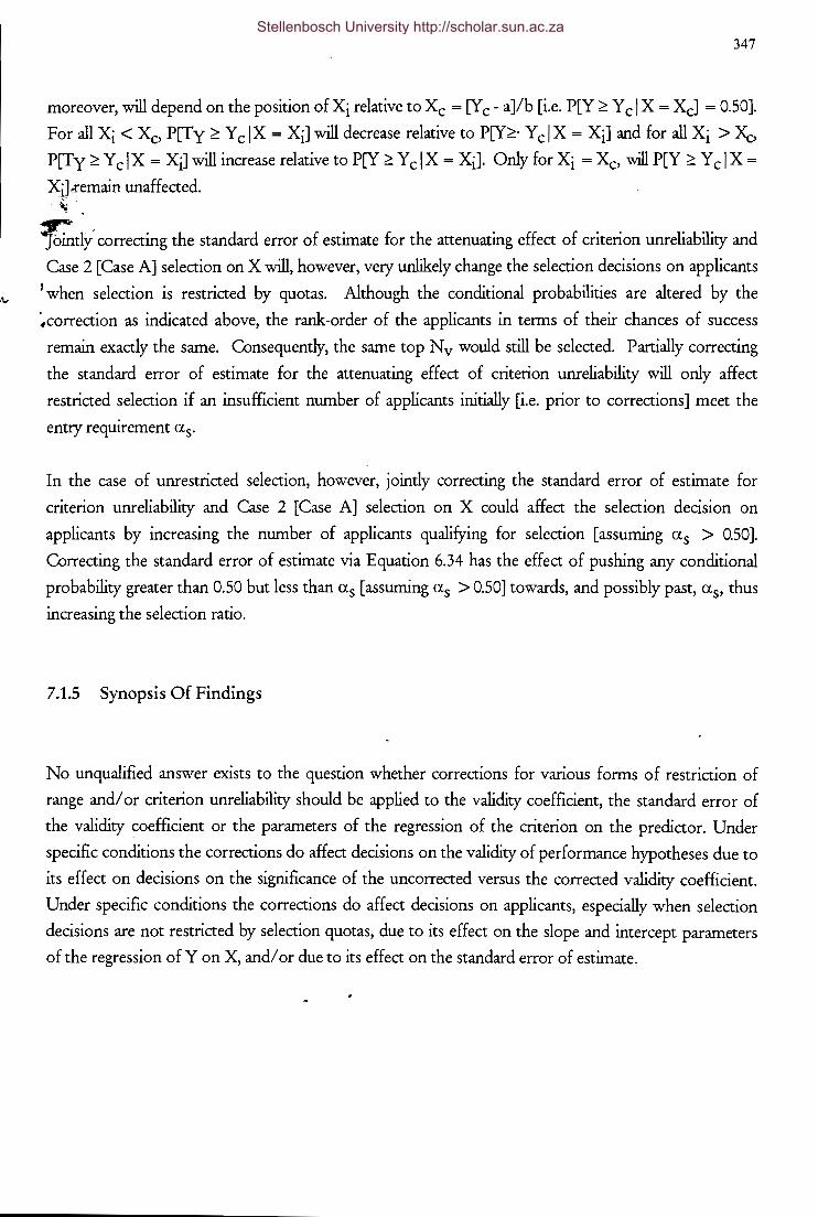
347
moreover, will depend on the position of Xi relative to Xc = [Y c- a]/b [i.e. P[Y ~ Y c I X = XcJ = 0.50].
For all Xi< Xc, P[Ty ~ Y c IX= Xi] will decrease relative to P[Y~· Yc I X= Xi] and for all Xi > Xo P[Ty ~ Y c I X = Xi] will increase relative to P[Y ~ Y c I X = Xi]. Only for Xi = X0 will P[Y ~ Y c I X=
XiJ.remain unaffected. '·. ~tly correcting the standard error of estimate for the attenuating effect of criterion unreliability and
Case 2 [Case A] selection on X will, however, very unlikely change the selection decisions on applicants 1 when selection is restricted by quotas. Although the conditional probabilities are altered by the
~correction as indicated above, the rank-order of the applicants in terms of their chances of success
remain exactly the same. Consequently, the same top Nv would still be selected. Partially correcting
the standard error of estimate for the attenuating effect of criterion unreliability will only affect
restricted selection if an insufficient number of applicants initially [i.e. prior to corrections] meet the
entry requirement as.
In the case of unrestricted selection, however, jointly correcting the standard error of estimate for
criterion unreliability and Case 2 [Case A] selection on X could affect the selection decision on
applicants by increasing the number of applicants qualifying for selection [assuming as > 0.50].
Correcting the standard error of estimate via Equation 6.34 has the effect of pushing any conditional
probability greater than 0.50 but less than as [assuming as > 0.50] towards, and possibly past, as, thus
increasing the selection ratio.
7.1.5 Synopsis Of Findings
No unqualified answer exists to the question whether corrections for various forms of restriction of
range and/ or criterion unreliability should be applied to the validity coefficient, the standard error of
the validity coefficient or the parameters of the regression of the criterion on the predictor. Under
specific conditions the corrections do affect decisions on the validity of performance hypotheses due to
its effect on decisions on the significance of the uncorrected versus the corrected validity coefficient.
Under specific conditions the corrections do affect decisions on applicants, especially when selection
decisions are not restricted by selection quotas, due to its effect on the slope and intercept parameters
of the regression of Y on X, and/ or due to its effect on the standard error of estimate.
Stellenbosch University http://scholar.sun.ac.za
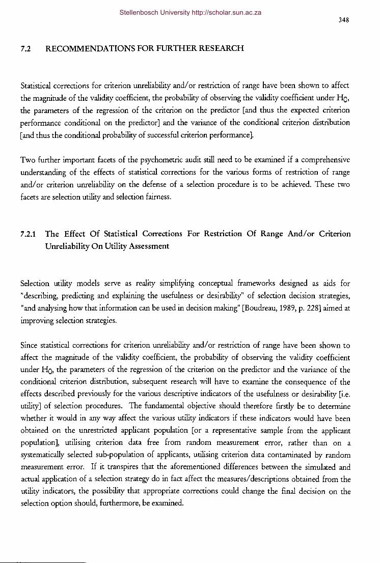
348
7.2 RECOMMENDATIONS FOR FURTHER RESEARCH
Statistical corrections for criterion unreliability and/ or restriction of range have been shown to affect
the magnitude of the validity coefficient, the probability of observing the validity coefficient under HQ,
the parameters of the regression of the criterion on the predictor [and thus the expected criterion
performance conditional on the predictor] and the variance of the conditional criterion distribution
[and thus the conditional probability of successful criterion performance].
Two further important facets of the psychometric audit still need to be examined if a comprehensive
understanding of the effects of statistical corrections for the various forms of restriction of range
and/ or criterion unreliability on the defense of a selection procedure is to be achieved. These two
facets are selection utility and selection fairness.
7.2.1 The Effect Of Statistical Corrections For Restriction Of Range And/ or Criterion
Unreliability On Utility Assessment
Selection utility models serve as reality simplifying conceptual frameworks designed as aids for
"describing, predicting and explaining the usefulness or desirability" of selection decision strategies,
"and analysing how that information can be used in decision making" [Boudreau, 1989, p. 228] aimed at
improving selection strategies.
Since statistical corrections for criterion unreliability and/ or restriction of range have been shown to
affect the magnitude of the validity coefficient, the probability of observing the validity coefficient
under HQ, the parameters of the regression of the criterion on the predictor and the variance of the
conditional criterion distribution, subsequent research will have to examine the consequence of the
effects described previously for the various descriptive indicators of the usefulness or desirability [i.e.
utility] of selection procedures. The fundamental objective should therefore firstly be to determine
whether it would in any way affect the various utility indicators if these indicators would have been
obtained on the unrestricted applicant population [or a representative sample from the applicant
population], utilising criterion data free from random measurement error, rather than on a
systematically selected sub-population of applicants, utilising criterion data contaminated by random
measurement error. If it transpires that the aforementioned differences between the simulated and
actual application of a selection strategy do in fact affect the measures/ descriptions obtained from the
utility indicators, the possibility that appropriate corrections could change the final decision on the
selection option should, furthermore, be examined.
Stellenbosch University http://scholar.sun.ac.za
349
The general question on how observed utility measures react to corrections for restriction of range
and/ or criterion unreliability seem to have received only very limited attention in the literature. The
question as to whether corrections for criterion unreliability and/ or various forms of restriction of
range should be applied in utility analysis had been acknowledged and discussed by several authors
[Cascio & Ramos, 1986; Schmidt, Hunter, McKenzie & Muldrow, 1979; Raju, N armand & Burke,
1990; Raju, Burke & Maurer, 199 5].
Schmidt, Hunter, McKenzie and Muldrow [1979, p. 612] express their position as follows:
The values of r[X,Y] and SDy should be those that would hold if applicants were hired randomly with
respect to test scores. That is they should be values applicable to the applicant population, the group in
which the selection procedure is actually used. Values of r{X,Y] and SDy computed on incumbents will
typically be underestimates because of reduced variance among incumbents on both test and job performance
measures." .... Values of rxy' should also be corrected for attenuation due to errors of measurement in the
criterion. Random error in the observed measure of job performance causes the test's correlation with that
measure to be lower than its correlation with actual job performance. Since it is the correlation Vlith actual
performance that determines test utility, it is the attenuation-corrected estimate that is needed in the utility
formulas.
Raju, Burke and Normand [1990, p. 6], however, disagree with the Schmidt, Hunter, McKenzie and
Muldrow [1979] position and maintain that
the psychometric validity of correcting the validity coefficient for unreliability in utility analysis needs to be
reassessed.
Ruju, Burke and Maurer [1995, pp. 143-144] similarly caution against an over-enthusiastic acceptance of
the aforementioned Schmidt, Hunter, McKenzie and Muldrow [1979] stance:
Although several authors have recognized the need for restriction of range corrections in utility analysis, there
has been little discussion of the underlying assumptions, and a critical evaluation of the necessity for
restriction of range corrections is lacking in the literature.
The objective of future research should be to provide precisely such a critical evaluation by examining
the consequences of correcting the various utility estimates for criterion unreliability and/ or r~striction
of range. In contrast to the foregoing citations, however, the analysis should not be restricted to the
Brogden-Cronbach-Gleser interpretation of selection utility. Rather than restricting the analysis to a
single interpretation of selection utility, the three definitions of payoff suggested by the Taylor-Russell,
the Naylor-Shine and the Brogden-Cronbach-Gleser utility models should be considered [Boudreau,
Stellenbosch University http://scholar.sun.ac.za
350
1991; Brogden, 1946; Brogden, 1949; Brogden & Taylor, 1950; Cronbach & Gieser, 1965; Naylor &
Shine, 1965; Taylor & Russell, 1993].
Future research should, in addition, examine the effect of corrections for restriction of range and/ or
criterion unreliability on the evaluation of the investment risk associated with selection procedures.
When viewed from a historical perspective, the evolution of selection utility models present a fairly
systematic progression from somewhat unsophisticated models to detailed, complex and rather
daunting contemporary models [Boudreau, 1991; Rauschenberger & Schmidt, 1987].
7.2.1.1 Payoff Defined In Terms Of The Validity Coefficient
The utility analysis model with the longest history defines payoff in terms of the validity coefficient. In
terms of this classical model, the utility of a [multiple regression] selection strategy is solely a function
of the correlation between a weighted, linear composite of predictors and a criterion measure.
Selection utility is thus equated with prediction accuracy defined in terms of the residual criterion
variance. Over- and underprediction are regarded as equally undesirable, irrespective of the position on
the criterion scale where they occur [Boudreau, 1991]. Two translations of the validity coefficient are
typically applied to convey its utility implications. The index of forecasting efficiency [Hull, 1928;
Kelley, 1923], E=[1-[1-p2]'h], indicates the proportional reduction in the standard error of estimate of
criterion scores predicted by the regression of the criterion on the weighted linear composite of
predictors compared to the standard error of estimate of criterion scores predicted by the criterion
mean [Boudreau, 1991; Guilford & Fruchter, 1978; Landy, Farr & Jacobs, 1982]. The coefficient of
determination, or the squared validity coefficient, reflects the proportion of variance in the criterion
measure accounted for by the weighted linear composite of selection predictors [Boudreau, 1991;
Guilford & Fruchter, 1978; Landy, Farr & Jacobs, 1982]. Both these indexes lead to the rather
disheartening conclusion that only selection strategies with validities exceeding those normally obtained
in validation studies, will have substantial practical utility. The fundamental problem with this line of
reasoning, however, lies in its complete disregard of the fact that criterion estimates are not desired as
an end in itself, but rather as necessary information required to arrive at a qualitative decision
[Cronbach & Gieser, 1965]. Precision in criterion estimation is important in human resource selection,
but only in as far as it affects the quality of decision-making.
The classical model's failure to formally acknowledge human resource selection as a form of decision
making, necessarily means that the structural elements characterising selection utility models can only
ex post facto be superimposed on it. When forced into a selection utility mold it could be argued,
Stellenbosch University http://scholar.sun.ac.za
351
albeit with some contention, that the classic model implicitly acknowledges decision options in as far as
it contrasts prediction based on test scores with chance results, implicitly acknowledges outcomes
characterised by the criterion [and therefore the quality attribute in a rudimentaty form] and implicitly
acknowledges the fact that the quality attribute of the outcome is [partially] a function of the validity
coefficient. The classical model, however, fails to, even implicitly, acknowledge the relevance of the
quantity and cost outcome attributes, the relevance of the situation in which the selection strategy is
used or the existence of a payoff function [total utility is simply equated to validity]. Despite serious
deficiencies, the proverbial baby should nevertheless not be thrown out with the bath water. If nothing
else, the logic underlying the classic model at least points to the seemingly still to often forgotten fact
that, in a human resource selection context, the focus of interest is not the selection instrument, but
rather the [evaluated] criterion. Far from being totally abandoned, the classical model in fact forms the
bedrock on which all other, more advanced, selection utility models are built. Boudreau [1991, p. 632]
attests to this point of view by stating:
Though the deficiencies inherent in these formulas are apparent when viewed from a decision-making
perspective, the fundamental notion of expressing the relationship between a predictor and a criterion in
terms of the correlation coefficient remains a basic building block of UA m:xlels. Later models began to
explore ways to embed the correlation coefficient within a set of decision attributes that made it easier to
interpret.
7.2.1.2 Payoff Defined In Terms OfThe Success Ratio
The Taylor-Russell utility model defines payoff in terms of the success ratio [Taylor & Russell, 1939].
In essence the Taylor-Russell model redefines the prediction problem as a task in predicting a
dichotomous criterion created through the formulation of a critical criterion cutoff score, thus reducing
the classical bivariate criterion-predictor distribution to a fourfold table [Ghiselli, Campbell & Zedeck,
1981; Taylor & Russell, 1939]. Such redefinition of the prediction problem acknowledges the fact,
overlooked by the classical model, that errors in prediction matter to the extent that they cause errors in
decisions [Cronbach & Gieser, 1965]. Prediction errors that matter, according to the Taylor-Russell
model, are only those where the expected and actual criterion scores fall on opposite sides of the
criterion cutoff thus either producing false positive decisions or false negative decisions [Ghiselli,
Campbell & Zedeck, 1981; Milkovich & Boudreau, 1994]. The primaty error to avoid, according to the
Taylor-Russell model, is to select applicants who actuarially should succeed but whose actual
performance fall below the minimally acceptable standard [i.e. false positive decisions]. The measure of
interest is therefore the success ratio, defined as the proportion of selected applicants who subsequently
do succeed as predicted [Boudreau, 1991].
Stellenbosch University http://scholar.sun.ac.za
352
The success ratio [Sv] varies as a function of the proportion of applicants in the applicant group that
would succeed on the criterion [i.e. Y ~ Y cJ should every applicant be selected [the base rate [BR ]1 the
proportion of applicants in the applicant group actually selected [the selection ratio [SR]] and p[X,Y]
[Blum & Naylor, 1968; Milkovich & Boudreau, 1994; Taylor & Russell, 1939].
The model, however, recognises that a high success ratio in itself is not sufficient to establish the
practical usefulness of a selection strategy. The Taylor-Russell model equates total utility with the
difference in the success ratio afforded by the selection procedure and the success ratio achieved when
selecting randomly from the applicant population [i.e. success ratio minus base rate]. The literature
generally indicates that the greatest absolute gain in prediction accuracy is achieved under conditions of
high predictive validity, low selection ratios and base rates approaching 0.50 [Blum & Naylor, 1968;
Boudreau, 1991; Milkovich & Boudreau, 1994]. Boudreau [1991, pp. 632-633], for example contends:
According to the Taylor-Russell tables, when other parameters are held constant, (a) higher validities produce
more improved success ratios (because the more linear the relationship, the smaller the area of the
distribution lying in the false-positive or false-negative region); (b) lower selection ratios produce more
improved success ratios (because lower selection ratios mean more "choosy" selection decisions, and the
predictor scores of selectees lie closer to the upper tail of the predictor distribution); and (c) base rate closer
to .50 produce more improved success ratios (because as one approaches a base rate of zero, none of the
applicants can succeed, thus, selection has less value; as one approaches a base rate of 1.0, all applicants can
succeed even without selection, so again, selection has less value).
However, when the behaviour of the Taylor-Russell payoff measure [i.e. the difference in the success
ratio afforded by the selection procedure and the success ratio achieved when selecting randomly from
the applicant population] is observed graphically over different possible combinations of values of BR,
SR and p[X,Y], such a straightforward conclusion seems unwarranted.
To the extent that the BR, SR and p[X,Y] can be influenced by the human resource function, through
changes in recruitment and revision of the selection strategy, it thus becomes possible to actively
manage the efficiency of the selection strategy. The Taylor-Russell utility model therefore challenges
the pessimism of the classical model on the practical usefulness of selection procedures with validities
in the 0.20- 0.50 range. Taylor and Russell [1939, p. 565-571] articulate their point of view as follow:
The wide-spread acceptance of such measures [as those advocated by the classical model; i.e. E and r"") as the
correct way of evaluating correlation coefficients has brought about a considerable pessimism with regard to
the validity coefficients which are ordinarily obtainable when tests are tried out in the employment office of a
business or industry or in an educational institution. We believe it may be of value to point out the very
considerable improvement in selection efficiency which may be obtained with small correlation coefficients.
Stellenbosch University http://scholar.sun.ac.za
353
The Taylor-Russell model formally acknowledges human resource selection as a form of decision
making. It still, however, ignores crucial structural elements of the basic selection utility model.
Although the Taylor-Russell model recognises the relevance of the situation in which the selection
strategy is used, and acknowledges the quality attribute of outcomes it still ignores both the quantity
and cost attributes [Boudreau, 1991; Boudreau, 1989]. The model's measure of quality is, furthermore,
bothersome because it firstly does not reflect natural units of value, and secondly, assumes the value of
performance to be equal at all points on the criterion scale above the criterion cutoff [Boudreau, 1991;
Cascio, 1991b].
7.2.1.3 Payoff Defined In Terms Of The Expected Standardised Criterion Score
The Naylor-Shine utility model defines payoff in terms of the expected standardised criterion score of
the selected group of applicants on the continuous criterion scale [Blum & Naylor, 1968; Cascio, 1991b;
Naylor & Shine, 1965], thereby amending the limitation of the Taylor-Russell utility model of not
reflecting the actual range of variation in selectee performance [Boudreau, 1991; Boudreau, 1989].
The Naylor-Shine model assumes a linear, homoscedastic regression of a normally distributed
standardised criterion [ZyJ on a normally distributed standardised predictor [ZxJ. Under these
assumptions, the expected standardised criterion score [E[ZY]] associated with a specific standardised
predictor score would be given by Equation 7.1 [Brogden, 1949; Naylor & Shine, 1965; Cronbach &
Gieser, 1965; Cascio, 1991 b; Boudreau, 1991 ]:
E[Z y] = p[X, Y]Z X --------------------------------------------------------------------------------------------- 7.1
This would then imply that, if the mean standardised predictor score of the selected group of applicants
was known, the expected mean standardised criterion performance of the selected group could be
found as the product of the validity coefficient and the mean standardised predictor score, as shown in
Equation 7.2:
E[E[Z y ]] = p[X, Y]E[Zx] --------------------------------------------------------------------------- 7.2
Brogden [1949] uses Equation 7.2 as the basic point of departure to show that the validity coefficient
indicates the ratio of the increase in criterion performance obtained by selecting above a given standard
predictor score to the increase that would be obtained by selecting above the same standard score on
the criterion itself. Therefore, if an increase of 8 in mean criterion performance could be obtained by
selecting the top n% on the criterion, an increase of p[X,Y]8 v.ould be obtained by selecting the top
Stellenbosch University http://scholar.sun.ac.za
354
n% on the predictor. Given the normality assumptions for the criterion and predictor, and given that
strict top-down selection can be assumed, the mean standardised predictor score of the top SR[100]%
of the applicant group would equal the product of the selection ratio and the height of the ordinate
under the normal distribution at the standardised predictor cutoff [A.], as shown in Equation 7.3
[Boudreau, 1991; Kelly, 1923; Naylor & Shine, 1965]:
E[Zx] = A.!SR --------------- --------7.3
Equation 7.2 can thus be rewritten as shown in Equation 7.4:
E[E[Zy ]] = p[X,Y](A./SR}---------------------------·-- ----7.4
Equation 7.4 returns the number of standard deviation units the selected group of applicants [assuming
strict top-down selection until the desired quota is reached] are expected to perform better on average
than a randomly selected group of the same size from the same applicant population. The Naylor
Shine utility model defines total utility in terms of Equation 7.4 as the difference in the mean
standardised criterion score between those applicants selected using the selection strategy in question
and those selected at random from the applicant population. This, however, has the disadvantage that
the unit in terms of which total utility is scaled is ill suited to assess the practical usefulness of a
selection strategy in a specific area of application. Transforming, through Equation 7.5, the gain
afforded by a selection procedure, expressed in standard deviation units, back to the original, raw score,
criterion scale would, to some extent, alleviate the difficulty of interpretation brought about by the
standardisation of the criterion scale.
E[E[YJsys]] - E[E[YJrandom]] = p[X, Y]cr[Y](A./SR}--------------------------------------7.5
The Naylor-Shine model, like the Taylor-Russell model, formally acknowledges human resource
selection as a form of decision-making. It also still ignores crucial structural elements of the basic
selection utility model. Although the Naylor-Shine model recognises the relevance of the situation in
which the selection strategy is used, and acknowledges the quality attribute of outcomes, it still ignores
both the quantity and cost attributes [Boudreau, 1991; Boudreau, 1989]. The model's measure of
quality is also troublesome because it still does not reflect natural units of value, although it assumes the
value of performance to vary over all points on the criterion scale [Boudreau, 1991; Cascio, 1991b].
Stellenbosch University http://scholar.sun.ac.za
355
7.2.1.4 Payoff Defined In Terms Of A Monetary Valued Criterion
The Brogden-Cronbach-Gleser [B-C-G] selection utility model defines payoff in terms of a monetary
valued criterion [Brogden, 1946; Brogden, 1949; Brogden & Taylor, 1950; Cronbach & Gleser, 1965].
The B-C-G selection utility model, similar to the Naylor-Shine model, assumes a linear, homoscedastic
regression of a normally distributed criterion [Y], scaled in an appropriate monetary unit, on a normally
distributed standardised predictor [ZxJ· Under these assumptions, the expected criterion score [E[Y]]
associated with a specific standardised predictor score would be given by Equation 7.6 [Brogden, 1949;
Cascio, 1991 b ]:
E[Y I z xJ = a + p z X --------------------------------------------------------------------------------------------------- 7. 6
Due to the aforementioned distribution assumptions underlying the B-C-G selection utility model, the
intercept a equals the mean criterion score of the applicant group [E[Y] and the regression coefficient
p equals the product of the validity coefficient and the ratio of the criterion and predictor standard
deviations [Tabachnick & Fidell, 1989]. The standard deviation of the standardised predictor, however,
by definition equals unity. Therefore Equation 7.6 can be rewritten as Equation 7.7:
E[Y 1 z xJ = E[Y] + p[X, YJSDy z x -------------------------------------------------------------------------------- 7.7
If the standardised predictor score fed into Equation 7.7 represents the mean standardised predictor
score of the selected applicant group and given E[Zx] = A.ISR, the absolute monetary value of the
mean criterion performance of the selected applicant group would be given by Equation 7.8:
E[Yisys] = E[Y] + p[X,Y]SDyE[Zx]
= E[Y] + p[X, Y]SDy[ A./ SR] ---------------------------------------------------------------------- 7. 8
Equation 7.8 states that the expected value of any new hire in the selected applicant group is the sum of
the value that would have resulted from random selection from the applicant pool and the incremental
value [i.e. per-selectee value] produced by systematic selection from the same applicant pool [Boudreau,
1991]. The monetary value of the increase in mean job performance afforded by the selection strategy
is given by Equation 7.9:
E[Yisys]- E[Y] = p[X,Y]SDyE[Zx]
= p[X,Y]SDy(A./SR) ------------------------------------------------------------------------- 7. 9
Stellenbosch University http://scholar.sun.ac.za
356
The marginal or incremental per-selectee utility of the once-off use of a selection procedure with a
validity coefficient p[X,Y] to select SR from an applicant group where a one-standard deviation
difference in monetary valued performance equals SDy at a per-applicant cost of C is given in
Equation 7.10:
L1U/selectee = (p[X,Y]SDy(A./SR))- (C/SR)-------------------------------------7.10
Conversely, the marginal or incremental per-testee utility is given by Equation 7.11 [Cronbach &
Gleser, 1965]:
flU/testee = p[X,Y]SDyA.- C
= flU I selectee[SR] ---------------------------------------------------------------------------------- 7.11
The total gain or utility attained from the once-off use of the selection procedure to select Ns selectees,
representing SR of the applicant group [NaJ, is given in Equation 7.12 [Brogden, 1949; Cronbach &
Gleser, 1965]:
flU = Ns{p[X,Y]SDy(A./SR) - (C/SR)}
= p[X,Y]SDy A.N a - CN a------------------------------------------------------------------- 7.12
The two versions of Equation 7.12 are numerically equivalent to each other. The first version of
Equation 7.12 reflects the Brogden [1949] argument and is stated in terms of the per-selectee utility
multiplied by the number of applicants selected. The second, Cronbach and Gleser [1965], version of
Equation 7.12 is derived by multiplying the per-applicant utility by the number of applicants.
A critical component of the B-C-G selection utility model is the standard deviation of monetary valued
job performance in the applicant population [SDy]. Accurate measurement of SDy is regarded as a
fundamental prerequisite for convincing and credible selection utility analyses. Despite its importance,
SDy continues to be a rather elusive quantity to estimate with satisfactory accuracy. The following
procedures have been proposed to estimate the standard deviation of the monetary valued criterion
[Boudreau, 1989; Boudreau, 1991; Cascio & Ramos, 1986; Cascio, 1991b; Cronbach & Gleser, 1965]:
~ cost accounting procedures;
~ global estimation procedures;
~ individual estimation procedures; and
~ proportional rules procedures.
Another, somewhat problematic term contained in the B-C-G selection utility model, is the validity
coefficient [p[X,Y]]. Strictly speaking the validity coefficient of interest to Equation 7.12 is the
correlation between the predictor and the monetary valued criterion. The monetary valued
Stellenbosch University http://scholar.sun.ac.za
357
performance scores are, however, relatively seldom available and only if a cost accounting or individual
estimation procedure is used to estimate SDy. Consequently the term p[X, Y] is interpreted as the
correlation between the predictor and a performance scaled criterion measure, under the assumption
that a linear, functional relationship exists between performance expressed in behavioral or output units
and performance expressed in monetary units. The assumption is thus made that the predictor
criterion correlation is not affected by the unit in terms of which the criterion is scaled [Boudreau,
1991; Hunter & Schmidt, 1982; Schmidt, Hunter, McKenzie & Muldrow, 1979].
Equation 7.12 [and Equation 7.10] shows that the efficiency of a selection strategy improves as the
validity coefficient increases, the monetary value of one standard deviation in performance increases,
cost of testing per selectee decreases and the selection ratio decreases. Utility is a positive linear
function of validity, and for zero cost, is proportional to validity [Brogden, 1946; Brogden, 1949]. For
any specific application SDy is a constant which indicates the magnitude and practical significance of
individual differences in monetary valued payoff [Cronbach & Gieser, 1965]. Although a decrease in
selection ratio increases the term A./SR [i.e. increases the average ability and performance of the
selectees], it at the same time increases the per-selectee cost. Equation 7.12 implies that total utility will
only be positive if the predictor cutoff is chosen such that the height of the ordinate under the normal
distribution [A.] at the cutoff would exceed the ratio of per-applicant cost to the product of the validity
coefficient and the standard deviation of the monetary valued criterion, that is if A > C/SDyp[X,Y]
[Cronbach & Gieser, 1965]. This would thus imply that for any C/SDyp[X,Y] >0.3989 utility must
necessarily be negative. For any positive value of C/SDyp[X,Y] < 0.3989 there exist two standardised
predictor scores, symmetrically positioned around the mean, defining a range of lambda values [and
therefore cutoff and SR values] which would satisfy the aforementioned expression
Increases in the validity coefficient and SDy would have the effect of pushing these critical cutoff
values to more extreme positions, thus permitting profitable selection with more extreme selection
ratios. This whole argument logically leads to the conclusion that the lowering of the selection ratio can
only benefit utility up to a point [Brogden, 1949]. Cronbach & Gieser [1965] demonstrated, through
differentiation of Equation 10 with respect to A, that the maximum utility per selectee is achieved for
the standardised predictor cutoff [ZxcJ that satisfies Equation 7.13:
A.- Zxc[SR] = C/(SDyp[X,Y])----------------------------------------------------------------7.13
If a fixed number of vacancies [NvJ need to be filled, the standardised predictor cutoff score that
satisfies Equation 13, would have to be translated to the required number of applicants to screen [Na;
Na = N/SR] so as to ensure that the optimum selection ratio equals the number of vacancies. If a
fixed number of vacancies need to be filled, per-selectee utility, as defined by Equation 10, and total
utility as, defined by Equation 7.12, would be maximised by determining the optimum standardised
Stellenbosch University http://scholar.sun.ac.za
358
predictor cutoff and optimum applicant group size through Equation 7.13 [Brogden, 1949; Cronbach &
Gieser, 1965]. If, however, no selection quota is in force [i.e. unrestricted selection] and with a fixed
number of applicants, Equation 7.12 indicates total utility to be a maximum if the selection ratio is fixed
at 0.50 [Cronbach & Gieser, 1965].
Equation 7.12 estimates the utility that would result within the first year from a single application of a
valid selection procedure, introduced where previously no procedure, or a totally invalid procedure, had
been used, to select a single cohort of selectees from an applicant population. The assumption that the
previous procedure can be equated to chance selection may be valid in some cases, but in other
situations the new procedure has to compete with a current/alternative procedure. Equation 7.12 can
be modified to accommodate this possibility as shown in Equation 7.14 [Cascio, 199lb; Cronbach &
Gieser, 1965; Schmidt, Hunter, McKenzie & Muldrow, 1979]:
~U = Ns{(p[X,YJt-p[X,Y]z)SDy(A./SR)- (C1-C2)/SR}
= (p[X,Y]1-p[X,Y]z)SDyA.N a- (C1-Cz)Na-------------------------------------------------7.14
Equation 7.12, furthermore, fails to acknowledge the fact that the benefits that accrue from the
selection of any single cohort of selectees are not limited to the first year after selection, but extends as
far into the future as the selectees remain in that particular position [Boudreau, 1991]. The costs
invested in the selection procedure generate returns to the organisation for as long as those selected
remain in the position they were selected into [Cranshaw & Alexander, 1985]. Failing to acknowledge
this, Equation 7.12 thus underestimates total utility. Equation 7.12 could, however, be modified to
make provision for the projected stream of future returns by incorporating the expected average tenure
[T] of the selectees into the equation and by assuming the stream of future returns to remain constant
over this time period as shown in Equation 7.15 [Boudreau, 1984; Boudreau, 1989]:
~U = Ns{Tp[X,Y]SDy(A./SR)]- C/SR}
= T p[X,Y]SDy A.N a - CN" a------------------------------------------------------------------------- 7.15
When evaluated from a decision-making perspective, the B-C-G selection utility model formally
acknowledges all crucial structural elements of the basic selection utility model [Boudreau, 1991;
Boudreau, 1989]. Thus all three outcome attributes are explicitly reflected; quantity through mean
tenure times number of applicants selected, quality through mean predictor score times validity
coefficient times monetary valued standard deviation and cost.
Stellenbosch University http://scholar.sun.ac.za
359
7 .2.1.5 Refining Payoff Defined In Terms Of A Monetary Valued Criterion
Boudreau [1983a; 1983b; 1989; 1991] pointed out that utility analyses guided by Equation 7.15 would,
however, still provide a distorted description of the monetcuy valued benefits that would result from
the implementation of a selection procedure. Such misrepresentation stems from the fact that
Equation 7.15 ignores economic considerations normally applied to other institutional financial
investment decisions [Boudreau, 1983a; Boudreau, 1983b; Boudreau, 1991; Clark, Hindelang &
Pritchard, 1984; Levy& Sarnat, 1994; Lumby, 1994]:
>- the tax liability faced by [most] organisations on the returns generated by the
investment in valid selection procedures;
>- the potential investment returns forfeited on future selection returns;
>- the effect of increased criterion performance on variable costs; and
>- the effect of employee flows produced by consecutive applications of a selection
procedure or the additive cohort effect.
By ignoring the combined effect of variable costs, taxes and the discounting of future earnings,
Equation 7.15 effectively stops short of fulfilling its promise of "providing the science of personnel
research with a more traditional 'bottom line' interpretation" [Landy, Farr & Jacobs, 1982, p. 38] of
institutional benefits comparable to the capital budgeting assessments applied to other, non-personnel,
investment options [Boudreau, 1983a; Cranshaw & Alexander, 1985]. Furthermore, by ignoring the
combined effects of variable costs, taxes and the discounting of future earnings, Equation 7.15
probably overestimates the total utility of a selection procedure. In contrast, however, by failing to
reflect the additive cohorts effect, Equation 7.15 will definitely underestimate the total utility of a
selection procedure [Boudreau, 1983b; Boudreau, 1991; Cascio, 1991b].
Boudreau's [1983a] concern with variable costs applies to utility analyses which scale the quality
attribute of institutional outcomes in terms of value of output, sales value or revenue. When a selection
strategy increases the quantity and/ or quality of output which, through its effect on sales value,
increases revenue but simultaneously increases/ decreases variable costs directly linked to increases
affected by the selection procedure [e.g. commission or piece rate remuneration, bonuses, employer
pension contributions, raw material costs, scrap or damages], the institutional benefit of such a
procedure can not be equated to the increase in sales value. Boudreau [1983a] thus argues that, because
a portion of the sacrifices an organisation must concede to produce output will be affected by the effect
of the selection procedure on performance, payoff should be defined in terms of the difference
between sales revenue and variable service costs or net institutional benefits. Fixed costs, in contrast,
do not affect utility estimates [i.e. the change in outcome expressed in terms of revenue or revenue
minus fixed costs would be the same], although they would lower the estimate of the mean profit
obtained from selected applicants if taken into account [i.e. it would have an effect on a variant of
Stellenbosch University http://scholar.sun.ac.za
360
Equation 5]. Since fixed costs by definition constitute a constant, correcting sales revenue for fixed
costs would not affect the monetary scaled standard deviation [SDy ], and therefore not the utility
estimate. Boudreau [1983a] proposes two possible avenues through which to include the effect of
selection procedures on variable cost in a selection utility model. Because relevant variable costs are
those correlating with the increase in sales value produced by the selection procedure, the extent of the
variable costs could be estimated by regressing service costs [SC] on the predictor [i.e. E[SC] =
[PX scJ[A./SR][SDscJJ and subtracting that from the original, sales revenue based, return estimate. '
Alternatively, by assuming variable costs to be proportional to sales revenue increases, change in net
institutional benefits could be obtained by factoring the variable costs component out of increased
revenue before adjusting for selection costs. This could be achieved through a parameter V, where V
equals the ratio of variable costs to sales revenue [SV], defining a term [1 + V] which is then
multiplicatively combined with the term Ns[T][px svJ[A./SR][SDsvJ before adjusting for selection costs '
[Boudreau, 1983a; Cascio, 1991b]. The parameter V becomes negative if the variable costs correlate
positively with sales revenue thus reducing the net benefit standard deviation [SDnb] from SDsv·
Boudreau [1983a] suggests a range of values for the parameter V from -.50 to .33 which implies an
adjustment ranging from .50 to 1.33.
Tax obligations are assessed on an organisation's reported profit. To the extent that improved selection
procedures contribute to increased profits it will also contribute to increased tax liability. Utility
estimates ignoring the impact of improved selection on tax liabilities would therefore overstate the net
institutional benefits derived from improved selection procedures. Because taxes are assessed on
reported profits, adjusting for taxes produces a proportional reduction in both revenue and selection
costs [Boudreau, 1983a]. The appropriate tax adjustment, given the preceding argument, is the tax rate
[TAX] applicable to the increase in reported profits attributable to improved selection [i.e. the marginal
tax rate]. The total utility estimate, after adjustment for variable costs, should thus be multiplied with
[1-TAX].
Selection procedures produce returns which accrue to the organisation over time. Equation 7.15
acknowledges this fact, but ignores the fact that returns received in different time periods are subject to
different opportunity costs [Boudreau, 1983a; Boudreau, 1991]. By simply adding the returns obtained
in future years to the returns obtained during the initial years, Equation 7.15 wrongfully equates future
monetary values with present monetary value thus ignoring the fact that immediately received returns
[and deferred costs] would/could be invested to earn interest [Boudreau, 1983a; Boudreau, 1991].
Returns received at different points in time should, therefore, first be converted to a common point in
time before accumulating the returns [Clark, Hindelang & Pritchard, 1984; Levy & Sarnat, 1994;
Lumby, 1994 ]. The present time constitutes such a common point. The net present value [NPV] of a
constant yearly stream of net benefits [At] generated overT years by investing in an improved selection
Stellenbosch University http://scholar.sun.ac.za
361
procedure applied once to select a single cohort of N s selectees, given a constant discount or interest
rate of i, is shown in Equation 7.16 [Clark, Hindelang & Pritchard, 1984; Lumby, 1994;]:
NPV = N s{L[At/ (1 + i)t]} -------------------------------------------------- 7.16
Building the effect of discounting into Equation 7.15 would require an estimate of the appropriate
discount rate. The discount rate in general flows from the implicit alternative to investing in a selection
procedure [or any other human resource intervention], namely lending the investment amount out on
the capital market at the market rate of interest [Lumby, 1994]. According to Boudreau [1983a, p. 566]:
the appropriate discount rate for utility analysis should be the rate applied to uninflated benefits and costs
given the organisation's evaluation of overall risk and return requirements ..... Because personnel programs
will be employed in all types of organisations from very risky endeavors to relatively risk-free endeavors, the
discount rate [i] must reflect the fact that risky firms must earn a risk premium and face a higher discount rate
than less risky firms.
Combining the effects of variable costs, taxes and the discounting of future earnings in Equation 7.15
produces Equation 7.17:
L\U = Ns{L[1/ (1 +i)t]}SDsv(l + V)(1-TAX)PXsv(A./SR) - C(l-T AX)-------------------------------- 7.17
Equation 7.17 reflects the fact that the costs of a selection procedure occur only at the stage of
selection and thus are not subject to discounting [Boudreau, 1983a]. Furthermore, Equation 7.17
assumes all parameters to remain constant over the T time periods. This assumption could readily be
relaxed by converting all relevant parameters that could be subject to change to variables, but that
would create the practical problem of estimating an appropriate array of values for each variable over
the T time periods.
Cranshaw and Alexander [1985] support the Boudreau [1983a] position that investments in human
resource interventions must be evaluated similarly to other investment options. Contraty to Boudreau
[1983a, 1983b], however, Cranshaw & Alexander [1985] do not propose any significant changes to the
basic B-C-G selection utility model [Equations 7.12 & 7.15], but rather suggest a number of capital
budgeting methods to follow on a point estimate of the expected return to the selection investment.
The following capital budgeting investment appraisal methods [Clark, Hindelang & Pritchard, 1984; Du
Plessis, 1986; Levy & Sarnat, 1994; Lumby, 1994] represent conceptual tools to integrate selection
utility into the broader financial decision-making processes within organisations:
>- pay-back period [PP];
>- return on investment [ROI];
Stellenbosch University http://scholar.sun.ac.za
);> net present value [NPV];
);> profitability index [PI]; and
);> internal rate of return [IRR].
362
The pay-back period [PP] is defined as the number of years an organisation requires to recover its
original investment from returns [Clark, Hindelang & Pritchard, 1984; Cranshaw & Alexander, 1985;
Lumby, 1994]. In selection investment applications, the pay-back period becomes especially relevant
for costly selection procedures applied to select a relatively small number of new hires into high
turnover jobs. Under these conditions there exists the real possibility that the pay-back period might
approach or exceed the expected tenure of the new cohort of hires; the selection procedure may
therefore not yield any real economic benefit to the organisation. Return on investment [ROI]
compares annual returns with the investment in the selection project. Net present value [NPV] is
defined as the difference between the discounted sum of the projected future returns and the total
amount invested. A projects NPV represents the increase/ decrease in return [i.e. excess return] that
would result from investing in the selection procedure rather than lending the investment amount on
the capital market at the market rate of interest. Consequently investment in any selection procedure
with a zero or positive NPV would be acceptable. A negative NPV project would be unacceptable
because it would make a loss relative to a capital market investment, it would produce a return less than
that available on the capital market and it would not generate sufficient returns to repay the financial
costs of undertaking it [Lumby, 1994]. The profitability index [PI] is defined as the ratio of the present
value of cash inflows to cash outflows. A ratio of one or greater, indicates that the yield of investing in
an improved selection procedure is equivalent to or greater than the discount rate [Clark, Hindelang &
Pritchard, 1984]. The internal rate of return [IRR] is defined as the rate which equates the net present
value of cash inflows with cash outflows. The IRR can thus be defined as the rate of discount which,
when applied to the selection investment's cash flow, would produce a zero NPV [lumby, 1994; Clark,
Hindelang & Pritchard, 1984]. Only projects with an IRR greater than the market rate of interest [or
any other cut-off rate] will be accepted [Lumby, 1994]. According to Cranshaw & Alexander [1985] the
aforementioned capital budgeting investment appraisal methods could be represented symbolically, in
terms of the Equation 7.15 version of the B-C-G selection utility model, as shown by Equations 7.18-
7.22:
PP = (C1 + Co)! {Nsp[X,Y]SDy(A./SR)} ------------------------------------------------------------------7.18
RO I = { {N s p[X,Y]SDy(A./ SR) }/ ( C 1 + Co])} 1 00 ------------------------------------------------------- 7.19
NPV = L { {N sP[X,Y]SDy (A./ SR) }r/[ 1 + k ]t} - ( C 1 + Co)-------------------------------------------------- 7. 20
PI = {L({Nsp[X,Y]SDy(A./SR) }r/ (1 +k)t) }/ (C1 +Co)---------------------------------------------7.21
IRR = j; L { {N s p[X,Y]SDy(A./ SR) }r/ ( 1 + j) t} = ( C 1 + Co) -------------------------------------------------- 7.22
Stellenbosch University http://scholar.sun.ac.za
363
Boudreau [1991] disagrees with the Crenshaw and Alexander [1985] formulations and suggests that
more consistent formulations would result if total returns [R] would be corrected by the
implementation costs [C1J before comparing it to the original costs [Co] of developing and validating
the selection procedure.
Equation 7.17, like all the B-C-G utility models preceding it, estimates total utility as the increase in
average monetary valued payoff resulting from adding a single cohort of selectees to the existing work
force through the use of a battery of predictors instead of random selection from the applicant
population. According to Boudreau [1983b; 1991], considering only a single cohort, however,
unnecessarily limits these utility models. Selection procedures are continuously reapplied as the
organisation expands and/ or employees move out of, or elsewhere in, the organisation. Organisations
do not invest in a selection procedure to use it once and then to discontinue its use, but rather to
continuously reapply the procedure to admit new members into the work force [Boudreau, 1991].
Thus, Boudreau [1983b] argues that the decision on the practical usefulness of a selection procedure
cannot be based on the results of a utility analysis focusing on a single application only. Equation 7.17,
and its B-C-G utility model predecessors, reflect the quantity attribute by multiplying the number hired
with the mean tenure of selectees [T]. Boudreau's [1983b] employee flows utility model, in contrast,
reflects quantity of employee-years of output in terms of the number of treated employees in the work
force [Nk], k time period in the future. The term Nk represents the end result of the combined effect
of the number of selected employees entering the work force [NatJ, the number of previously selected
employees leaving the work force [NstJ and the average tenure of employees selected into the
organisation [i.e. Nk = L[N at-N stJ; t= 1, 2, ... , k]. For any given time period t = q, 1 < q < k, utility is
still reflected by the product of quantity[Nq]times quality[p[X,Y][SDy][A-/SR] minus cost. To obtain
a total utility estimate these separate time period utility estimates are summed over all future time
periods [k= 1, 2, ... , F]. Boudreau's [1983b; 1991] employee acquisition flows utility model is formally
explicated in Equation 7.23:
~U = L(L(Nat-NsJ){(l/(1+i)k)SDsv(l+ V)(1-TAX)rx.sv(A-/SR)}-
L { Ck( 1-TAX) { 1/ ( 1 + i) (k -1)} }-------------------------------------------------------- 7.23
The classic B-C-G utility formulations [Equation 7.12] have been modified to apply to performance
enhancing human resource interventions [e.g. training or performance feedback] following on selection
[Florin-Thuma & Boudreau, 1987; Landy, Farr & Jacobs, 1982; Mathieu & Leonard, 1987; Schmidt,
Hunter & Pearlman, 1982] by substituting the product [SDy ][p[X, Y]] reflecting the difference in
average criterion performance between systematically and randomly selected applicants expressed in
standard deviation units, with d, the difference in criterion performance between the treated and
untreated groups, expressed in standard deviation units. All subsequent developments on the basic B
C-G formulation [Equations 7.14, 7.15 ,7.17 & 7.23] apply equally well, in their modified form, to
Stellenbosch University http://scholar.sun.ac.za

364
human resource interventions aimed at improving employee performance in their existing assignments
[Milkovich & Boudreau, 1994].
A noticeable shortcoming in the utility analysis approaches discussed thus far, is their inability to
account for human resource management activities preceding selection [i.e. recruitment] and employee
separation [i.e. layoffs, retirement, quits & dismissals]. Boudreau and Rynes [1985], and Boudreau and
Berger [1985] addressed this shortcoming by proposing modifications of Equation 7.23 that would
integrate the effects of recruitment and selection into a single decision-theoretic utility model
[Boudreau, 1991; Boudreau & Rynes, 1985] and by developing a utility model that could encompass not
only the effects of employee acquisitions but also of employee separations [Boudreau, 1991; Boudreau
& Berger, 1985a].
All versions of the basic B-C-G selection utility model discussed thus far, scaled utility as the difference
from an unknown utility level that would have resulted if the selection strategy would not have been
used. All versions of the basic B-C-G selection utility model discussed thus far, also assumed that all selection strategy options would be implemented within the same applicant population [Boudreau,
1991]. The latter assumption implies that all selection options considered are teamed up with the same
recruitment strategy. If this would not be the case, any one of the B-C-G selection utility models
discussed thus far, could provide a misleading indication of the most beneficial selection option
because it would ignore the effects of the recruitment strategy it is teamed up with on the applicant
pool [Boudreau & Rynes, 1985; Boudreau, 1991]. The recruitment strategy, specifically the recruitment
method, the nature of the recruitment message, the nature and level of required applicant qualifications
and the nature of administrative procedures [Boudreau & Rynes, 1985], could influence the size of the
applicant pool as well as the parameters of the marginal criterion and predictor distributions in the
applicant population. The recruitment strategy could therefore influence all parameters of the B-C-G
selection utility models discussed thus far. Thus Boudreau and Rynes [1985] argue that a particular
recruitment strategy-selection strategy combination could produce the greatest total value, although the
selection procedure of choice may offer a lower incremental utility relative to other selection options, if
the recruitment strategy produces a substantial increase in the average applicant value. To express
utility in absolute terms Boudreau and Rynes [1985] essentially add the incremental utility afforded by
the selection option under consideration to the expected value of the discounted, after cost, after tax
monetary valued payoff resulting from random selection from the recruited applicant pool. Boudreau
and Rynes [1985] proposed three changes to Equation 7.23 to reflect the combined effect of
recruitment and selection on utility. They firstly introduced a variable Crk to represent the cost
associated with a particular recruitment strategy [r] that generates the applicant pool from which Nak
new hires are selected in time period k. They secondly introduced a term [jtsvr-P.scr] to represent the
average after-cost service/ sales value of the recruited applicant pool. The third modification proposed
by Boudreau and Rynes [1985] was to formally change the status of p[X,Y], A-/SR, SDy and C from
Stellenbosch University http://scholar.sun.ac.za
365
constants to variables with values contingent on the recruitment strategy employed. The expected
value of the discounted, after-cost, after tax monetary valued payoff from using selection procedure x
under recruitment strategy r, evaluated for F future periods is given by Equation 7.24:
E[U]x,r = p::(1/1+i)kp:(Nat-NsJ(PX.svr)(ZXr)(SDsvr)(1+ V)} +
:E(1/1 +i)kp:(Natr-Nstr)(j.tsvrJLscr)} -
:E( 1 I 1 + i) (k -1) ( Csk +Ctk)} ( 1-TAX) -------------------------------------------------- 7. 2 4
Significant similarity exist between employee acquisitions through selection procedures and employee
separations through quits, layoffs and dismissals [Boudreau, 1991 ]. Both processes involve employee
movement across the organisational boundary [Boudreau & Berger, 1985a]. Furthermore, both
processes in essence refer to a procedure whereby a subset of employees is selected from a larger
"applicant" pool. Human resource selection procedures acquire subsets of employees from a larger
applicant pool outside the organisation while human resource separation procedures select subsets of
employees from a larger pool of current employees to remain in the organisation [Boudreau & Berger,
1985a; Milkovich & Boudreau, 1994]. Boudreau and Berger [1985] exploited these similarities between
employee acquisitions and employee separations to develop an external employee movement utility
model that could encompass the effects of both processes. The multiple-cohort acquisition and
retention utility model [Boudreau & Berger, 1985a] estimates the absolute utility of the work force,
rather than the incremental utility added by, procedures designed to regulate employee movement
across organisational boundaries, under any one of the following three possible scenarios:
~ repeated acquisitions without separations over time [i.e. the work force is
systematically increased through selection];
~ repeated unreplaced separations over time [i.e. the work force is systematically
reduced through separations]; and
~ repeated separations and acquisitions over tune [i.e. the work force is either
maintained, increased or reduced depending on the number of employees entering
and leaving during each time period].
The multiple-cohort acquisition and retention utility model [Boudreau & Berger, 1985a] essentially
integrates two distinct utility models; a repeated selection utility [or multiple cohort acquisition] model
estimating the discounted, after-cost, after-tax work force value that would result in a pure growth
situation and a repeated separation [or multiple cohort retention] utility model estimating the
discounted, after-cost, after-tax work force value that would result in a pure shrinkage situation. The
multiple cohort acquisition utility model estimates total work force value by firstly estimating the work
force value at the beginning of the analysis as the number of incumbent employees [Nio] in the period
prior to the implementation of the selection procedure times their quality [i.e. their mean service value
minus the mean service costs associated with that force [svo-sco]]. The implementation of a selection
Stellenbosch University http://scholar.sun.ac.za
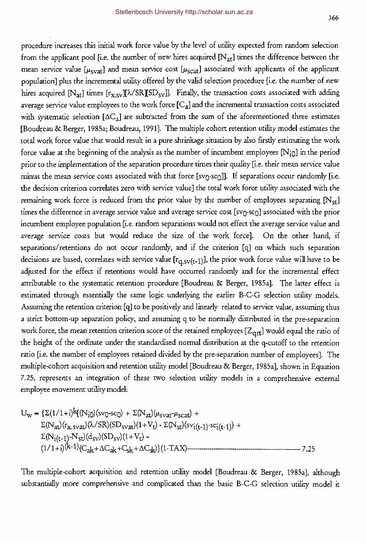
366
procedure increases this initial work force value by the level of utility expected from random selection
from the applicant pool [i.e. the number of new hires acquired [N ad times the difference between the
mean service value [J.tsvad and mean service cost [J.tscad associated with applicants of the applicant
population] plus the incremental utility offered by the valid selection procedure [i.e. the number of new
hires acquired [NatJ times [rx.svJ[A./SR][SDsvJJ. Finally, the transaction costs associated with adding
average service value employees to the work force [CaJ and the incremental transaction costs associated
with systematic selection [~CaJ are subtracted from the sum of the aforementioned three estimates
[Boudreau & Berger, 1985a; Boudreau, 1991]. The multiple cohort retention utility model estimates the
total work force value that would result in a pure shrinkage situation by also firstly estimating the work
force value at the beginning of the analysis as the number of incumbent employees [NioJ in the period
prior to the implementation of the separation procedure times their quality [i.e. their mean service value
minus the mean service costs associated with that force [svo-sco]]. If separations occur randomly [i.e.
the decision criterion correlates zero wit~ service value] the total work force utility associated with the
remaining work force is reduced from the prior value by the number of employees separating [NstJ
times the difference in average service value and average service cost [ svo-sco] associated with the prior
incumbent employee population [i.e. random separations would not effect the average service value and
average service costs but would reduce the size of the work force]. On the other hand, if
separations/ retentions do not occur randomly, and if the criterion [ q] on which such separation
decisions are based, correlates with service value [rq.sv(t-1)], the prior work force value will have to be
adjusted for the effect if retentions would have occurred randomly and for the incremental effect
attributable to the systematic retention procedure [Boudreau & Berger, 1985a]. The latter effect is
estimated through essentially the same logic underlying the earlier B-C-G selection utility models.
Assuming the retention criterion [ q] to be positively and linearly related to service value, assuming thus
a strict bottom-up separation policy, and assuming q to be normally distributed in the pre-separation
work force, the mean retention criterion score of the retained employees [ZqrtJ would equal the ratio of
the height of the ordinate under the standardised normal distribution at the q-cutoff to the retention
ratio [i.e. the number of employees retained divided by the pre-separation number of employees]. The
multiple-cohort acquisition and retention utility model [Boudreau & Berger, 1985a], shown in Equation
7.25, represents an integration of these two selection utility models in a comprehensive external
employee movement utility model:
Uw = {L(1/1+i)k[(Nio)(svo-sco) + L(NaJVtsvat-J.tscaJ +
L(NaJ(rx.svaJ(A./SR)(SDsvaJ(1+ VJ- L(NsJ(svi(t-1)-SCi(t-1)) +
~~iitD R ~ s(~~:)~~;~gs:: ~~4J} ( 1-TAX)--------------------------------------------------- 7.25
The multiple-cohort acquisition and retention utility model [Boudreau & Berger, 1985a], although
substantially more comprehensive and complicated than the basic B-C-G selection utility model it
Stellenbosch University http://scholar.sun.ac.za
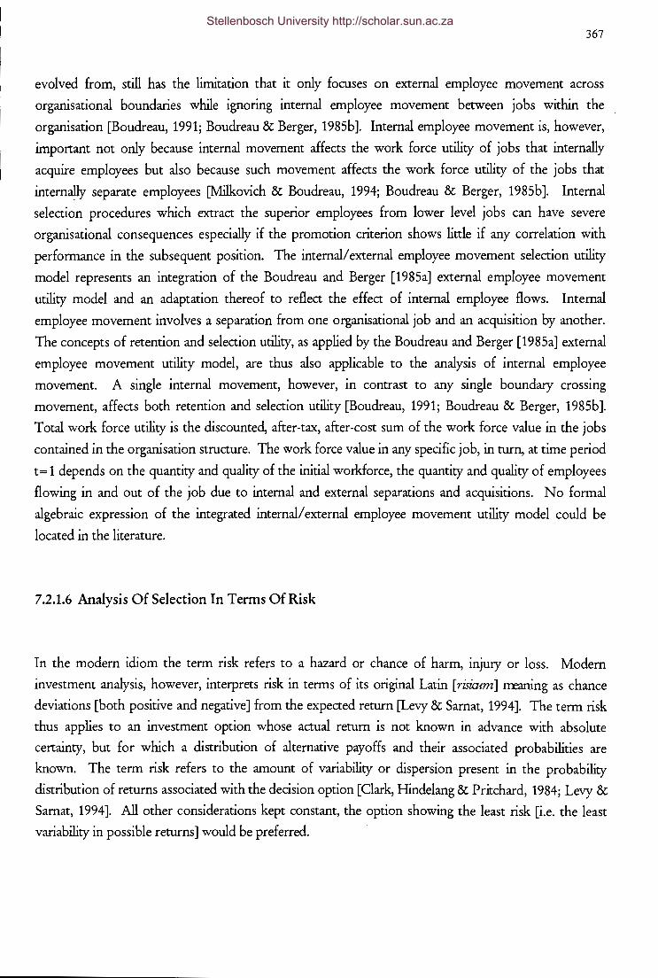
367
evolved from, still has the limitation that it only focuses on external employee movement across
organisational boundaries while ignoring internal employee movement between jobs within the
organisation [Boudreau, 1991; Boudreau & Berger, 1985b]. Internal employee movement is, however,
important not only because internal movement affects the work force utility of jobs that internally
acquire employees but also because such movement affects the work force utility of the jobs that
internally separate employees [Milkovich & Boudreau, 1994; Boudreau & Berger, 1985b ]. Internal
selection procedures which extract the superior employees from lower level jobs can have severe
organisational consequences especially if the promotion criterion shows little if any correlation with
performance in the subsequent position. The internal/ external employee movement selection utility
model represents an integration of the Boudreau and Berger [1985a] external employee movement
utility model and an adaptation thereof to reflect the effect of internal employee flows. Internal
employee movement involves a separation from one organisational job and an acquisition by another.
The concepts of retention and selection utility, as applied by the Boudreau and Berger [1985a] external
employee movement utility model, are thus also applicable to the analysis of internal employee
movement. A single internal movement, however, in contrast to any single boundary crossing
movement, affects both retention and selection utility [Boudreau, 1991; Boudreau & Berger, 1985b].
Total work force utility is the discounted, after-tax, after-cost sum of the work force value in the jobs
contained in the organisation structure. The work force value in any specific job, in turn, at time period
t= 1 depends on the quantity and quality of the initial workforce, the quantity and quality of employees
flowing in and out of the job due to internal and external separations and acquisitions. No formal
algebraic expression of the integrated internal/ external employee movement utility model could be
located in the literature.
7 .2.1.6 Analysis Of Selection In Terms Of Risk
In the modern idiom the term risk refers to a hazard or chance of harm, injury or loss. Modem
investment analysis, however, interprets risk in terms of its original Latin [risiatm] rreaning as chance
deviations [both positive and negative] from the expected return [Levy & Sarnat, 1994]. The term risk
thus applies to an investment option whose actual return is not known in advance with absolute
certainty, but for which a distribution of alternative payoffs and their associated probabilities are
known. The term risk refers to the amount of variability or dispersion present in the probability
distribution of returns associated with the decision option [Clark, Hindelang & Pritchard, 1984; Levy &
Samat, 1994]. All other considerations kept constant, the option showing the least risk [i.e. the least
variability in possible returns] would be preferred.
Stellenbosch University http://scholar.sun.ac.za
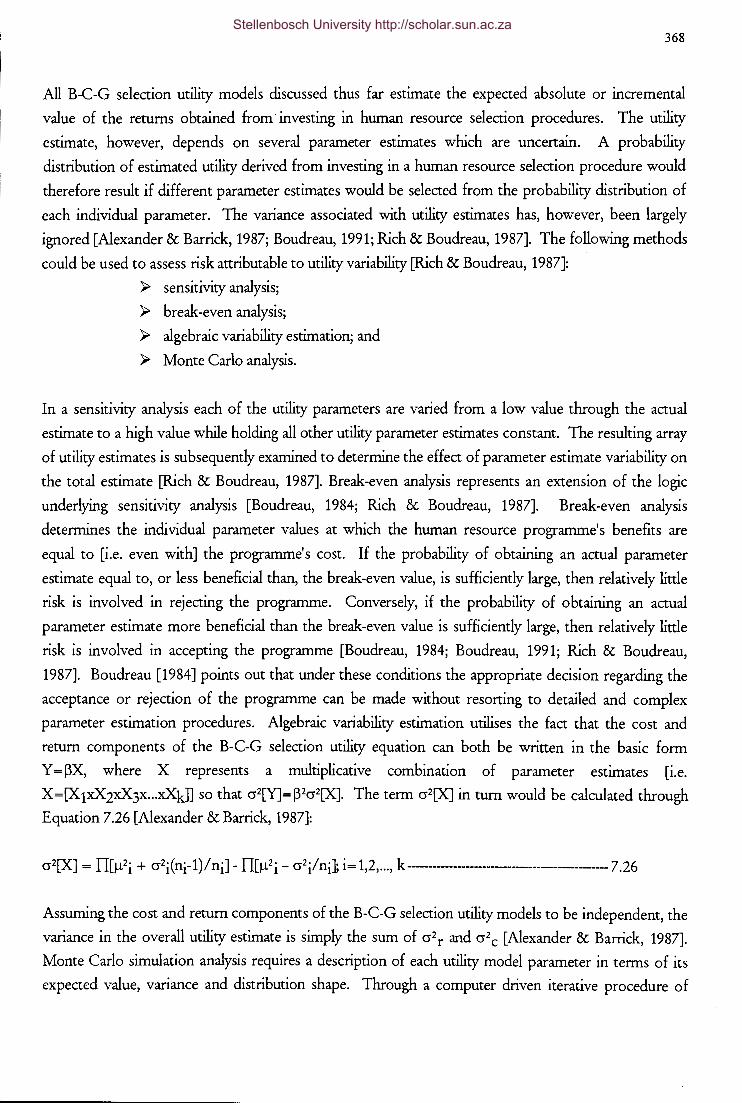
368
All B-C-G selection utility models discussed thus far estimate the expected absolute or incremental
value of the returns obtained from· investing in human resource selection procedures. The utility
estimate, however, depends on several parameter estimates which are uncertain. A probability
distribution of estimated utility derived from investing in a human resource selection procedure would
therefore result if different parameter estimates would be selected from the probability distribution of
each individual parameter. The variance associated with utility estimates has, however, been largely
ignored [Alexander & Barrick, 1987; Boudreau, 1991; Rich & Boudreau, 1987]. The following methods
could be used to assess risk attributable to utility variability [Rich & Boudreau, 1987]:
);> sensitivity analysis;
);> break-even analysis;
);> algebraic variability estimation; and
);> Monte Carlo analysis.
In a sensitivity analysis each of the utility parameters are varied from a low value through the actual
estimate to a high value while holding all other utility parameter estimates constant. The resulting array
of utility estimates is subsequently examined to determine the effect of parameter estimate variability on
the total estimate [Rich & Boudreau, 1987]. Break-even analysis represents an extension of the logic
underlying sensitivity analysis [Boudreau, 1984; Rich & Boudreau, 1987]. Break-even analysis
determines the individual parameter values at which the human resource programme's benefits are
equal to [i.e. even with] the programme's cost. If the probability of obtaining an actual parameter
estimate equal to, or less beneficial than, the break-even value, is sufficiently large, then relatively little
risk is involved in rejecting the programme. Conversely, if the probability of obtaining an actual
parameter estimate more beneficial than the break-even value is sufficiently large, then relatively little
risk is involved in accepting the programme [Boudreau, 1984; Boudreau, 1991; Rich & Boudreau,
1987]. Boudreau [1984] points out that under these conditions the appropriate decision regarding the
acceptance or rejection of the programme can be made without resorting to detailed and complex
parameter estimation procedures. Algebraic variability estimation utilises the fact that the cost and
return components of the B-C-G selection utility equation can both be written in the basic form
Y = px, where X represents a multiplicative combination of parameter estimates [i.e.
X=[X1xX2xX3x ... xXkJJ so that cr2[Y]=P2cr2[X]. The term cr2[X] in tum would be calculated through
Equation 7.26 [Alexander & Barrick, 1987]:
Assuming the cost and return components of the B-C-G selection utility models to be independent, the
variance in the overall utility estimate is simply the sum of cr2r and cr2c [Alexander & Barrick, 1987].
Monte Carlo simulation analysis requires a description of each utility model parameter in terms of its
expected value, variance and distribution shape. Through a computer driven iterative procedure of
Stellenbosch University http://scholar.sun.ac.za
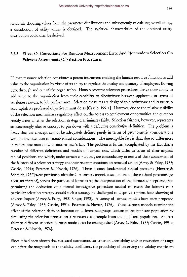
369
randomly choosing values from the parameter distributions and subsequently calculating overall utility,
a distribution of utility values is obtained. The statistical characteristics of the obtained utility
distribution could then be derived.
7.2.2 Effect Of Corrections For Random Measurement Error And Nonrandom Selection On
Fairness Assessments Of Selection Procedures
Human resource selection constitutes a potent instrument enabling the human resource function to add
value to the organisation by virtue of its ability to regulate the quality and quantity of employees flowing
into, through and out of the organisation. Human resource selection procedures derive their ability to
add value to the organisation from their capability to discriminate between applicants in terms of
attributes relevant to job performance. Selection measures are designed to discriminate and in order to
accomplish its professed objective it must do so [Cascio, 1991a]. However, due to the relative visibility
of the selection mechanism's regulatory effect on the access to employment opportunities, the question
readily arises whether the selection strategy discriminates fairly. Selection fairness, however, represents
an exceedingly elusive concept to pin down with a definitive constitutive definition. The problem is
firstly that the concept cannot be adequately defmed purely in terms of psychometric considerations
without any attention to moral/ ethical considerations. The inescapable fact is that, due to differences
in values, one man's foul is another man's fair. The problem is further complicated by the fact that a
number of different definitions and models of fairness exist which differ in terms of their implicit
ethical positions and which, under certain conditions, are contradictory in terms of their assessment of
the fairness of a selection strategy and their recommendations on remedial action [Arvey & Faley, 1988;
Cascio, 1991a; Petersen & Novick, 1976]. Three distinct fundamental ethical positions [Hunter &
Schmidt, 197 6] were previously identified. A fairness model, based on one of these ethical positions [or
a variant thereof], serves the purpose of formalising the interpretation of the fairness concept and thus
permitting the deduction of a formal investigative procedure needed to assess the fairness of a
particular selection strategy should such a strategy be challenged to disprove a prima facie showing of
adverse impact [Arvey & Faley, 1988; Singer, 1993]. A variety of fairness models have been proposed
[Arvey & Faley, 1988; Cascio, 1991a; Petersen & Novick, 1976]. These fairness models examine the
effect of the selection decision function on different subgroups contain in the applicant population by
simulating the selection process on a representative sample from the applicant population. At least
thirteen different selection fairness models can be distinguished [Arvey & Faley, 1988; Cascio, 1991a;
Petersen & Novick, 1976].
Since it had been shown that statistical corrections for criterion unreliability and/ or restriction of range
can affect the magnitude of the validity coefficient, the probability of observing the validity coefficient
Stellenbosch University http://scholar.sun.ac.za

370
under Ho, the parameters of the regression of the criterion on the predictor and the variance of the
conditional criterion distribution, subsequent research should examine how these effects impact on the
judgments delivered on the fairness of selection procedures by various selection fairness models. The
fundamental objective of future research in this regard should therefore be to determine whether the
finding/verdict of the various fairness models when applied to a specific selection strategy and their
recommendations on remedial action, if required, would change as a result of these corrections.
At least three of the aforementioned array of fairness models [Petersen & Novick, t976] should be
formally examined in terms of their reaction to statistical corrections for restriction of range and/ or
criterion unreliability, namely:
>- the regression or Cleary model;
>- the equal risk or Einhorn-Bass model; and
>- the constant ratio or Thorndike model.
7.2.2.t The Cleary Model Of Selection Fairness
The regress10n or Cleary model of selection fairness defines fairness in terms of differences in
regression slopes and/ or intercepts across the subgroups [1tt and 1t2] comprising the applicant
population [Arvey & Faley, t988;; Cascio, t99ta; Maxwell & Arvey, t993; Petersen & Novick, t976].
According to Cleary [ t968, p. ttS]:
A test is biased for members of a subgroup of the population if, in the prediction of the criterion for which
the test was designed, consistent nonzero errors of prediction are made for members of the subgroup. In
other words, the test is biased if the criterion score predicted from the common regression line is consistently
too high or too low for members of the subgroup. With this definition of bias, there may be a connotation
of unfair, particularly if the use of the test produces a prediction that is too low. If the test is used for
selection, members of a subgroup may be rejected when they were capable of adequate performance.
The Cleary model examines the fairness of a selection strategy by fitting a saturated regression equation,
exemplify by Equation 7.28 shown below, and testing the hypothesis Hot= B2=B3=0 against the
alternative hypothesis Ha: at least one of the two parameters is not zero [Berenson, Levine &
Goldstein, t983; Kleinbaum & Kupper, t978]. Should Hot not be rejected it would imply the use of
the common regression equation to be fair. Should Hot, however, be rejected it would imply the use
of the common regression equation to be unfair because it would imply the separate regression
equations to differ in terms of slope and/ or intercept [i.e. one would have to conclude that the
regression models fitted to the two subgroups are not coincident].
Stellenbosch University http://scholar.sun.ac.za
E[YIXJ= a+ P1X + P2D + P3X"rD-------------------------------------------7.28
Where D denotes a dummy variable, coded such that:
D = 0 for group 1t1
D = 1 for group 7t2
371
The appropriate remedy, should the latter situation prevail, is contingent on the explanation for the
rejection of Ho. The Cleary model's prescription for a diagnosed unfair selection strategy thus depends
on whether there exists an equivalent incremental difference in criterion performance across applicants
from the two subgroups, regardless of predictor performance [i.e. P2 * 0, but the interaction parameter
P3 can be assumed zero] or a non-equivalent incremental difference in criterion performance across
applicants from the two subgroups, dependent on the ability level of the applicants [i.e. there exists a
subgroup x predictor performance interaction effect on criterion performance; P3 * 0] [Berenson,
Levine & Goldstein, 1983; Kleinbaum & Kupper, 1978]. The Cleary solution to the fairness problem
thus dictates that the information category entries in the strategy matrix [Cronbach & Gieser, 1965]
should be derived from an appropriately expanded multiple regression equation containing the
grouping variable as a main effect and/ or in interaction with the predictor.
7.2.2.2 The Einhom-Bass Model Of Selection Fairness
The equal risk or Einhorn-Bass selection fairness model operationalises the concept in terms of
differences in the probability of success conditional on predictor performance [i.e. a selection strategy
would be considered unfair if P[Y~YciXi,7!I] * P[Y~YciXi,1t2] for all i] [Cascio, 1991a; Einhorn &
Bass, 1971; Petersen & Novick, 1976]. The Einhorn-Bass conceptualisation thus corresponds to the
Guion [1966, p. 26] definition of unfair discrimination:
Unfair discrimination exists when persons with equal probabilities of success on the job have unequal
probabilities of being hired for the job.
The equal risk model would therefore judge any selection strategy unfair should it be considered unfair
by the Cleary model. In addition, however, it would also consider the selection strategy unfair if the
criterion variance conditional on predictor performance differs across the two applicant subgroups [i.e.
cr2[Y IX; 7t1] * cr2[Y IX; n2]] [Cascio, 1991a; Einhorn & Bass, 1971; Petersen & Novick, 1976]. The
Einhorn-Bass solution to the fairness problem thus dictates that the information category entries [i.e.
P[Y~ Y c I Xi,7tj]] in the strategy matrix [Cronbach & Gieser, 1965] should be obtained by deriving
Stellenbosch University http://scholar.sun.ac.za
372
E[Y I Xi;7tj] from the appropriate regression equation and subsequently, transforming Y c to a standard
score in the conditional criterion distribution [assuming normality] by using the appropriate standard
error of estimate as denominator [Berenson, Levine & Goldstein, 1983; Einhorn & Bass, 1971;
Kleinbaum & Kupper, 1978].
7.2.2.3 The Thorndike Model Of Selection Fairness
The constant ratio or Thorndike model of selection fairness considers a selection strategy fair if it
selects the same proportion of applicants from the various applicant subgroups that would qualify for
selection on the basis of the criterion [Cascio, 1991a; Petersen & Novick, 1976; Thorndike, 1971].
Thorndike [1971, p. 63] approaches the question of selection fairness from a group perspective when
he proposes that in a fair selection strategy: /
the qualifying scores on a test should be set at levels that will qualify applicants in the two groups in
proportion to the fraction of the two groups reaching a specified level of criterion performance.
The most generic interpretation of the constant ratio model would be to consider a selection strategy
fair if the ratio of the selection ratio to the base rate would be equal across the subgroups of the
applicant population [Petersen & Novick, 1976]. Should a selection strategy be judged unfair towards a
specific subgroup the solution to the fairness problem, according to the constant ratio model, would be
to adjust the predictor cutoff scores [Thorndike, 1971].
7.2.2 Additional Specific Recommendations For Further Research
In addition to examining the effect of corrections for restriction of range and/ or criterion unreliability
on utility and fairness assessments, future research should also examine:
~ the effect of corrections for restriction of range and/ or criterion unreliability on the
standard errors of the regression coefficients and standard error of estimate of the
regression of Y on X;
~ the effect of joint corrections for Case C restriction of range and criterion
unreliability on the validity coefficient, the standard error of the validity coefficient,
the empirical exceedence probability, the slope and intercept parameters of the
regression of Y on X and the standard error of estimate;
Stellenbosch University http://scholar.sun.ac.za

373
>- the correlation p[E[TyiX],Ty1 relative to p[X,Y], p[X,Ty], and p[Tx,Ty]and its
standard error;
>- the effect of Case 2 [Case A] restriction of range on Y on the parameters of the
regression of Y on X.
Future research should also extend the analyses in chapter 6 to the multiple regression model. The
effect of corrections for restriction of range and/ or criterion unreliability on selection decision-making
should also be examined from the perspective of alternative selection strategies.
Stellenbosch University http://scholar.sun.ac.za
374
REFERENCES
Alexander, R.A. [1988]. Group homogeneity, range restriction, and range enhancement effects on
correlations. PersannelPsyclxJ~, 41, 773-777.
Alexander, R.A. & Barrick, MR. [1987]. Estimating the standard error of projected dollar gains in utility
analysis. journal of AppliRdPsydxJ~, 72 [3], 475-479.
Allan, N.L. & Dunbar, S.B. [1990]. Standard errors of correlations adjusted for incidental selection.
AppliRd Psyd;oforjad Measurrmmt, 14 [1], 83-94.
American Psychological Association. [1954]. Technical recommendations for psychological tests and
diagnostic techniques. Psychoforjad Bulletin, 51 [2,Pt. 2].
American Psychological Association. [1966]. Standards for ffiucational and psyd;olagical tests and manuals.
Washington, DC: Author.
American Psychological Association, American Educational Research Association & National Council
on Measurement in Education. [ 197 4 ]. Standards for educational and psyd;oforjad tests.
Washington; American Psychological Association.
American Psychological Association, American Educational Research Association & National Council
on Measurement in Education. [1985]. Standards for ed:ucational and psycholagical tests.
Washington; American Psychological Association.
Angoff, W.H. [1953]. Test reliability and effective test length. Psydxmetrika, 18 [1], 1-14.
Arvey, R.D. & Faley, R.H. [1988]. Fairness in selectingemfinyees [Second edition]. Reading, Mass.: Addison
Wesley.
Austin, J.T. & Villanova, P. [1992]. The criterion problem: 1917-1992. journal of AppliRdPsydxJlo~, 77 [6],
836-874.
Babbel, D.F., Stricker, R. & Vanderhoof, LT. [1994]. A modem approach to performance measurement
for insurers. In R.L. D'Ecclesia & S.A. Zenios [Eds.]. OJErations researr:h, mxlels in
quantitatil:e foumce. Heidelberg: Physica-Verlag.
Babbie, E. [1989]. 7he practice of socid researr:h [Fifth edition]. Belmont, California: Wadsworth Publishing
Company.
Barrett, G.V., Phillips, J.S. & Alexander, R.A. [1981]. Concurrent and predictive validity designs: a critical
reanalysis. journal of AppliedPsydxJ~, 66 [1], 1-6.
Berenson, M.L., Levine, D.M. & Goldstein, M. [1983]. Internurliate statistical metha/s and applications; a
a:mputerpackageapprvcuh. Englewood Cliffs, New Jersey: Prentice Hall.
Binning, J.F. & Barrett, G.V. [1989]. Validity of Personnel decisions: a conceptual analysis of the
inferential and evidential bases. journal of AppliRd PsyclxJ~, 7 4 [3], 478-494.
Blum, M.L. & Naylor, J.C. [1968]. Industrial psyd;o~: its throretical and socid foundations. New York: Harper
&Row.
Bobko, P. [1983]. An analysis of correlations corrected for attenuation and range restriction. journal of
AppliRdPsycho~, 68 [4], 584-589.
Stellenbosch University http://scholar.sun.ac.za

375
Bobko, P. & Rieck, A. [1980]. Large sample estimators for standard errors in functions of correlation
coefficients. Applial Psychola;jcal Measurrment, 4 [3], 385-398.
Boone, J.O. & Lewis, M.A. [1980]. Demonstration of possible effects of recruitment and selection
procedures on correcting the validity coefficient for restriction of range. Psycholo/}cal
Reparts, 46, 927-930.
Boudreau, J.W. [1983a]. Economic considerations in estimating the utility of human resource
productivity improvement programs. Personnel PsycholrYgy, 36, 551-576.
Boudreau, J.W. [1983b]. Effects of employee flows on utility analysis of human resource productivity
improvement programs. journal of ApplialPsychology, 68 [3], 396-406.
Boudreau, J.W. [1984]. Decision theory contributions to HRM research and practice. Industrial Relations,
23 [2], 198-217.
Boudreau, J.W. [1989]. Selection utility analysis: a review and agenda for further research. In M. Smith &
I. Robertson [Eds. ]. Adrunres in selection coul assessmmt. Chichester: John Wiley & Sons.
Boudreau, J.W. [1991]. Utility analysis for decisions in human resource management. In M.D. Dunnette
& L.M. Hough [Eds.]. Handlmk of industrid coul organizational psychology [Second edition;
Volume 2]. Palo Alto, California: Consulting Psychologists Press, Inc.
Boudreau, J.W. & Berger C.J. [1985a]. Decision-theoretic utility analysis applied to employee separations
and acquisitions. journal of Applial Psychology, 70 [3], 581-612.
Boudreau, J.W. & Berger, C.J. [1985b]. Towards a model of employee movement utility. In K.M
Rowland & G.R. Ferris [Eds.]. Research in personnel and human resources managpnent [Volume
3]. Greenwich, Connecticut: JAI Press Inc.
Boudreau, J.W. & Rynes, S.L. [1985]. Role of recruitment in staffing utility analysis. Journal of Applial
Psychology, 70, 354-366.
Boyatzis, R.E. [1982]. 1he amjX!tentmanager. New York: Wiley.
Brogden, H.E. [1946]. On the interpretation of the correlation coefficient as a measure of predictive
efficiency. 1he Journal of Educational Psychology, 37, 65-76.
Brogden, H.E. [1949]. When testing pays off. PersonndPsychology, 2, 171-183.
Campbell, J.P. [1991]. Modeling the performance prediction problem in industrial and organizational
psychology. In M.D. Dunnette & L.M. Hough [Eds.]. Handlook of industrial coul
organizational psychology [Second edition; Volume 1 ]. Palo Alto, California: Consulting
Psychologists Press, Inc.
Campbell, D.T. & Stanley, J.C. [1963]. Experimentd andquasi-experimmtal desiff1S far research. Chicago: Rand
McNally College Publishing Company.
Carnap, R. [1950]. Logjcal fcundation of probahility. Chicago: University of Chicago Press.
Cascio, W.F. [1991a]. Applial psychology in personnel rna~. Englewood Cliffs, N.J.: Prentice-Hall.
Cascio, W.F. [1991b]. Costing human resources; the foumcial impact of behavior in organizations. Boston: PWS-
Kent Publishing Company.
Cascio, W.F. & Ramos, R. [1986]. Development and application of a new method for assessing job
performance in behavioral/ economic terms. journal of Applial Psychofc.w, 1, 20-28.
Stellenbosch University http://scholar.sun.ac.za
376
Clark, J.J., Hindelang, T.J. & Pritchard, RE. [1984]. Capital budg;ting; p&nning and control of capital
expenditures. Englewood Cliffs, New Jersey: Prentice Hall.
Cleary, T.A. [1968]. Test bias: prediction of grades of Negro and white students in integrated colleges.
]ounwl of Educatimal Measu'Yf111ml, 5, 115-124.
Cohen, J. [1977]. Statistiml pac.eer analysis far the behavioral scieru:es [Revised edition]. New York: Academic
Press.
Cohen, J. & Cohen, P. [1983]. Appli£dmultiple ngressionlcarrelatinn analysis far the behavioral scieru:es. Hillsdale,
New Jersey: Lawrence Erlbaum Associates Publishers.
Cook, T.D. & Campbell, D.T. [1979]. Qtasi-experimentation: desi'i!JZ and analysis issues far field settings. Chicago:
Rand McNally.
Cook, T.D., Campbell, D.T. & Peracchio, L. [1991]. Quasi experimentation. In M.D. Dunnette & L.M
Hough [Eds.]. Handlmk of industrial and organizational psycho/ugJ [Second edition; Volume
2]. Palo Alto, California: Consulting Psychologists Press, Inc.
Coombs, [1950]. A theory of data. New York: Wiley and Sons.
Copi, I.M. & Cohen, C. [1990]. Intrrxluction to bgjc. New York: Macmillan Publishing Company.
Coxon, A.P.M. [1982]. The user's gjtide tornultidinunsion scaling. London: Heinemann Educational Books.
Crocker, L. & Algin a, J. [ 1986]. Intrrxluaion to classiml and malem test theory. New York: Holt, Rinehart and
Winston.
Cronbach, L. [1951]. Coefficient alpha and the internal structure of tests. Psychom:trika, 16 [3], 297-333.
Cronbach, L.J. & Gieser, G.C. [1965]. Psychohgjcal tests and personnel da:isions [2nd edition]. Urbana, Illinois:
University of Illinois Press.
Cronbach, L.J., Gieser, G.C., Nanda, H. & Rajaratnam, N. [1972]. The dependability of behavioral
measunments. New York: John Wiley.
Cranshaw, S.F. & Alexander, RA. [1985]. One answerto the demand for accountability: selection utility
as an investment decision. Organizational Behavior and HUl11d}1, Docision Processes, 35, 102-118.
Crous, M.J. [1986]. Personeelbestuur. In P.G. Du Plessis [Red.]. TGefi1Jasde btdryfsekanonie: n inleidende
oorsig. Pretoria: HAUM Uitgewery.
Diaconis, P.M. & Efron, B.S. [1983]. Computer-intensive methods in statistics. Scientific American, 116-
130.
Dobson, P. [1988]. The correction of correlation coefficients for restriction of range when restrictions
result from the truncation of a normally distributed variable. British ]ounwl of Mathematical
and Statistiml Psycho/ugJ, 41, 227-234.
Drasgow, F. & Hulin, C.L. [1991]. Item response theory. In M.D. Dunnette & L.M Hough [Eds.].
Handl::wk of industrid and organizational psycho/ugJ [Second edition; Volume 2]. Palo Alto,
California: Consulting Psychologists Press, Inc.
Duvenage, A. [1991]. A heuristic on the validity generalization dilanma. HSRC Report R/Pers 786. Pretoria:
Human Sciences Research Council.
Efron, B.S. [1982]. The jackknife, the bJotstrap and other resampling plans. Philidelphia: Society for Industrial
and Applied Mathematics.
Efron, B.S. [1988]. Bootstrap confidence intervals: good or bad? Psychohgjcal Bulletin, 104, 293-296.
Stellenbosch University http://scholar.sun.ac.za
377
Efron, B.S. & Gong, G. [1983]. A leisurely look at the bootstrap, the jackknife and cross-validation. The
American Statistician, 37 [1], 36-48.
Efron, B.S. & Tibshirani, R.J. [1986]. Bootstrap methods for standard errors, confidence intervals and
other measures of statistical accuracy. Statistical Science, 1, 54-7 4.
Efron, B.S. & Tibshirani, R.J. [1993]. An intrrxluaionto thlrotstrap. New York: Chapman and Hall.
Einhorn, H.J. & Bass, A.R. [1971]. Methodological considerations relevant to discrimination m
employment testing. Psychdagjad Bulletin, 75 [4], 261-269.
Ellis, M.V. & Blustein, D.L. [1991]. Developing and using educational and psychological tests and
measures: the unificationist perspective. journal ofOJunseling and Deulopnent, 69, 550-555.
Feldt, L.S. [1975]. Estimation of the reliability of a test divided into two parts of unequal length.
Psychcmetrika, 40 [4], 557-561.
Feldt, L.S. & Brennan, R.L. [1989]. Reliability. In R.L. Linn [Ed.]. Educational Me£~Surrment [Third Ed.].
New York: American Council on Education.
Fitz-Enz, J. [1980]. Quantifying the human resource function. Personnel, 57 [3, 41-52.
Florin-Thuma, B.C. & Boudreau, J.W. [1987]. Performance feedback utility in a small organization:
effects on organizational outcomes and managerial decision processes. Personnel Psycf.,ology,
40, 693-713.
Forsythe, R.A. [1971]. An empirical note on a correlation coefficient corrected for restriction of range.
Educational and Psycf.,ofutjcal Measurrment, 31, 115-123.
Forsyth, A. & Feldt, L.S. [1969]. An investigation of empirical sampling distributions of correlatiot"
coefficients corrected for attenuation. Educational and Psycf.,ofutjcal Measurrment, 29, 61-71.
Gatewood, R.B. & Feild, H.S. [1994]. Hum:mresourresela:tion. Fort Worth: The Dryden Press.
Ghiselli, E.E., Campbell, J.P. & Zedeck, S. [1981]. Measurrment tlxmy for the behauioural sciences. San
Francisco: W.H. Freeman and Company.
Gilmer, J.S. & Feldt, L.S. [1983]. Reliability estimation for a test with parts of unknown lengths.
Psychcmetrika, 48 [1], 99-111.
Gow, J.F. [1985]. Human Resource managers must remember the bottom line. Pe~ journal, 30-32.
Greener, J.M. & Osburn, H.G. [1980]. Accuracy of corrections for restriction in range due to explicit
selection in heteroscedastic and nonlinear distributions. Educational and Psycf.,oln;jcal
Measurrment, 40, 337-346.
Gross, A.L. [1982]. Relaxing the assumptions underlying corrections for restriction of range. Educational
and Psycf.,ofutjcal Measunment, 42, 795-801.
Gross, A.L. [1990]. A maximum likelihood approach to test validation with missing and censored
dependent variables. Psychonebika, 55 [3], 533-549.
Gross, A.L. & Fleishman, L. [1983]. Restriction of range corrections when both distribution and
selection assumptions are violated. Applied Psycf.,oln;§cal Measurrment, 7 [2], 227-23 7.
Gross, A.L. & Kagen, E. [1983]. Not correcting for restriction of range can be advantageous. Educational and Psycf.,ofutjcal Measunment, 43, 389-396.
Gross, A.L. & McGanney, M.L. [1987]. The restriction of range problem and non-ignorable selection
processes. Journal of AppliedPsycf.,ology, 72 [ 4], 604-610.
Stellenbosch University http://scholar.sun.ac.za
378
Gross, A.L. & Su, W. [1975]. Defining a fair or unbaised selection model: a question of utilities. Journal of
AppliadPsydxJ!ogy, 60 [3], 345-351.
Guilford, J.P. & Fruchter, B. [1978]. Fundamental statistics in psydxJ!ogy and e:lucatilm. T ckyo: McGraw-Hill.
Guion, R.M. [1965]. Personnel testing. New York: McGraw-Hill Book Company.
Guion, R.M. [1966]. Employment tests and discriminatory hiring. IndustriaL Relations, 5, 20-37.
Guion, R.M. [1991]. Personnel assessment, selection and placement. In M.D. Dunnette & L.M Hough
[Eds.]. HandlxxJk of industrial and mganizational psydxJ!ugy [Second edition; Volume 2]. Palo
Alto, California: Consulting Psychologists Press, Inc.
Guion, R.M. & Cranny, C.J. [1982]. A note on concurrent and predictive validity designs: a critical
reanalysis. ]oumal of AppliedPsydxJ!ogy, 67 [2], 239-244.
Gulliksen, H. [1950]. Thoory of mental tests. New York: John Wiley and Sons.
Gullickson, A & Hopkins, K. [1976]. Interval estimation of correlation coefficients corrected for
restriction of range. Educational and Psycl:vlagjcal Measurcmmt, 36, 9-25.
Guttman, L. [1945]. A basis for analyzing test-retest reliability. Psydxmetrika, 10 [ 4], 255-282.
Hakstian, A.R., Schroeder, M.L. and Rogers, W.T. [1988]. Inferential procedures for correlation
coefficients corrected for attenuation. Psydxmetrika, 53 [1], 27-43.
Hakstian, A.R., Schroeder, M.L. and Rogers, W.T. [1989]. Inferential theory for partially disattenuated
correlation coefficients. Psydxmetrika, 54 [3], 397-407.
Hambleton, R.K. [1989]. Principles and selected applications of item response theory. In R.L. linn [Ed.].
Educational Measumnent [Third Ed.]. New York: American Council on Education.
Hanges, P.l., Rentsch, JR., Yusko, K.P. & Alexander, RA. [1991]. Determining the appropriate
correction when the type of range restriction is unknown: developing a sample-based
procedure. Educational and PsydxJ!agjcal Measumnent, 51, 329-340.
Hays, W.L. [1971]. Statistics for the social sciences [second edition]. Londom: Holt, Rinehart and Winston.
Held, J.D. & Foley, P.P. [1994]. Explanations for accuracy of the general multivariate formulas in
correcting for range restriction. Appliad PsydxJ!agjcal Measumnent, 18 [ 4], 355-367.
Holmes, D.J. [1990]. The robustness of the usual corrections for restriction in range due to explicit
selection. Psydxmetrika, 55 [1], 19-32.
Horst, P. [1951]. Estimating the total test reliability from parts of unequal length. Educational and
PsydxJ!agjcal Measumnent, 11, 368-371.
Hoyt, C. [1941]. Test reliability estimated by analysis of variance. Psydxmetrika, 6 [3], 1941.
Huber, G.P. [1980]. Manatpiddrosionmaking. Glenview, illinois; Scott, Foresman.
Huck, S.W. [1992]. Group heterogeneity and Pearson's r. Educational andPsydxJla;§cal Measumnent, 52, 253-
260.
Hull, C.L. [1928]. Aptitude testing. Yonkers, NY: World Book.
Hunter, J.E. & Schmidt, F.L. [1976]. Critical analysis of the statistical and ethical implications of various
definitions of test bias. PsydxJ!agjcal Bulletin, 83 [6], 1053-1071.
Hunter, J.E. & Schmidt, F.L. [1982]. Fitting people to jobs: the impact of personnel selection on national
productivity. In M.D. Dunnette & E.A. Fleischman [Eds.j. Human perfonnance and
~[Vol. 1, pp.233-284]. Hillsdale, New Jersey: Erlbaum.
Stellenbosch University http://scholar.sun.ac.za
379
Hunter, J.E., Schmidt, F.L. & Jackson, G.B. [1982]. Meta-analysis: cumulating research findings across studies.
Beverly Hills, CA.: Sage.
Johnston, J.T. & Ree, M.J. [1994]. Rangej: a Pascal program to compute the multivariate correction for
range restriction. Educatimd and Psycholo;jcd Measurerrmt, 54 [3], 693-695.
Kane, M.T. [1992]. An argument-based approach to validity. Psycholo;jcd Bulletin, 112 [3], 527-535.
Keats, J.A. [1957]. Estimation of error variances of test scores. Psy:lxmetrika, 22, 29-41.
Keeney, R.L. & Raiffa, H. [197 6]. Docisions with multiple obj£rtil£s: preferences and wlue tradmffs. New York:
John Wiley & Sons.
Kelley, T.L. [1923]. Statistical metlxxl. New York: The MacMillan Company.
Kelley, T.L. [1947]. Fundarrmtds of statistics. Cambridge: Harvard University Press.
Kendall, M.G. & Stuart, A. [1977]. The adu:mad throry of statistics [Vol. 1, Fourth ed.]London: Charles
Griffm and Company.
Kerlinger, F.N. [1986]. Foundationsofbehauiouralresearr:h. New York: CBS Publishing.
Kleiman, L.S. & Faley, R.H. [1985]. The implications of professional and legal guidelines for court
decisions involving criterion related validity: a review and analysis. Persarrnel Psyc!xJ/agy, 38,
803-833.
Kleinbaum, D.G. & Kupper, L.L. [1978]. Applied regression analysis and other multiv:zriate metlxxls. North
Sciituate, Mssachusetts: Duxbury Press.
Kristof, W. [1974]. Estimation of reliability and true score variance from a split of a test into three
arbitrary parts. Psy:lxmetrika, 39 [ 4], 491-499.
Kristof, W. [1982]. qontributions to the analysis of carrelationaxfficients. Unpublished doctoral dissertation,
University of South Africa, Pretoria.
Kuder, F. [1991]. Comments concerning the appropriate use of formulas for estimating the internal
consistency reliability of tests. Educational and Psycholofia::d Measururzmt, 51, 873-87 4.
Kuder, G.F. & Richardson, M.W. [1937]. The theory of the estimation of test reliability. Psy:}xmet:rika, 2
[3], 151-160.
Landy, F.J. [1986]. Stamp collecting versus science; validation as hypothesis testing. American Psycho/a;!jst, 41 [11], 1183-1192.
Landy, F.J., Farr, J.L. & Jacobs, R.R. [1982]. Utility concepts in performance measurement. Orgnizational Behavior and Humctn Peiforrruoue, 30, 15-40.
Lawsche, C.H. & Balma, M.J. [1966]. Principles of personnel testing. New York: McGraw-Hill Book
Company.
Lee, R. & Foley, P. [1986]. Is the validity of a test constant throughout the test score range?. joumal of ' Applied Psychology, 71 [4], 641-644.
Lee, R., Miller, K.J. & Graham, W.K. [1982]. Corrections for restriction of range and attenuation in
criterion-related validation studies. journal of Applied Psychology, 67 [5], 637-639.
Levin, J. [1972]. The occurrence of an increase in correlation by restriction of range. Psy:lxmetrika, 37 [1],
93-97.
Levy, H. & Sarnat, M. [ 1994 ]. Capital inu:stmmt and .financial decisions. New York: Prentice Hall.
Stellenbosch University http://scholar.sun.ac.za
380
Linn, R.L. [1968]. Range restriction problems in the use of self-selected groups for test validation.
Psy::hola;jad Bulletin, 69 [1], 69-73.
Linn, R.L. [1983]. Pearson selection formulas: implications for studies of predictive bias and estimates of
educational effects in selected samples. journal of Educational Measurrment, 20 [ 1 ], 1-15.
Linn, R.L., Harnish, D.L. & Dunbar, S.B. [1981]. Corrections for range restriction: an empirical
investigation of conditions resulting in conservative corrections. joumal of Applicd
Psy::holagj, 66 [6], 655-663.
Lipsey, M.W. [1990]. Design sensitivity; statistical pau:er for experimental researdJ. Newbruy Park, California:
Sage Publications.
Lord, F.M. & Novick, M.R. [1968]. Statistical theories of mental test scores. Reading, Massachusetts: Addison
Wesley Publishing Company.
Lumby, S. [ 1994 ]. !mf!Stment appraisal and financial da:isirns [Fifth edition]. London: Chapman & Hall.
Lunneborg, C.E. [1985]. Estimating the correlation coefficient: the bootstrap approach. Psy:hola;jad
Bulletin, 98, 209-215.
March, J.G. & Simon, H. G. [1958]. Organizations. New York; Wily.
Margenau, H. [ 19 50]. 7he nature of pJ.rysical m:zlity. New York: McGraw-Hill.
Marx, F.W. [1983]. Personeelbestuur. In F.W. Marx & P.J. Van Aswegen [Reds.]. Die bedryfsekonanie: n kart oorsig. Pretoria: HAUM Uttgewety.
Maxwell, S.E. & Arvey, R.D. [1993]. The search for predictors with high validity and low adverse impact:
compatible or incompatible goals?. journal of ApplialPsy::holagj, 78 [3], 433-437.
Mayer, J.D. Estimating the sampling variance of correlation corrected for attenuation using coefficient
alpha. Perceptual and Motor Skills, 56, 207-210.
McGuire, D.P. [1986]. The occurrence of an increase in correlation with explicit selection. Psydxmetrika,
51 [2], 331-333.
McGuire, W.J. [1997]. Creative hypothesis generating in psychology: some useful heuristics. Annual
ReuiewofPsy::holagj, 48, 1-30.
Mendoza, J.L. [1993]. Fisher transformations for correlations corrected for selection and missing data.
Psydxmet:rika, 58 [4], 601-615.
Mendoza, J.L. & Mumford, M. [1987]. Corrections for attenuation and range restriction on the predictor.
journal of Educational Statistics, 12 [3], 282-293.
Mendoza, J.L., Hart D.E. & Powell, A. [1991]. A bootstrap confidence interval based on a correlation
corrected for range restriction. Multiu:triate Behauioral Researrh, 26 [2], 255-269.
Messick, S. [1989]. Validity. In RL. Linn [Ed.]. Educational mM.SUrrment [Third edition]. New York:
American Council on Education and McMillan Publishing Company.
Milkovich, G.T. & Boudreau, J.W. [1994]. Human rescurce managpnent [Seventh edition]. Homewood,
Illinois: Richard D. Irwin Inc.
Moran, P.A.P. [1970]. On asymptotically optimal tests of composite hypothesis. Bi011Wika, 57 [1], 47-55.
Mouton, J. & Marais, H.C. [1985]. Metxxlolagje wn die gresteSJ:W!!enskappe: basiese bfgYippe. Pretoria:Raad vir
Geesteswetenskaplike N avorsing.
Stellenbosch University http://scholar.sun.ac.za
381
Muchinsky, P.M. [1983]. Psychofuty appliRd to 'lWYk; an intraluction to industrid and organizationd psychofuty.
Homewood, Illinois; The Dorsey Press.
Naylor, J.C. & Shine, L.C. [1965]. A table for determining the increase in mean criterion score obtained
by using a selection device. journal of Industrial Psucholagy, 3, 33-42.
Novick, M.R. [1966]. The axioms and principal results of classical test theory. Journal of Matlxmatical
Psycho/ngJ, 3, 1-18.
Novick, M.R. & Lewis, C. [1967]. Coefficient alpha and the reliability of composite measurements.
Psychcmetrika, 32 [1], 1-13.
Nunnally, J.C. [1978]. Psyclxmetric theory. New York: McGraw-Hill Book Company.
Olson, CA. & Becker, B.E. [1983]. A proposed technique for the treatment of restriction of range in
selection validation. Psycho/a;!jcal Bulletin, 93 [1], 137-148.
Owen, K. & Taljaard, J.J. [1988]. Pretoria: Human Sciences Research Council
Pearson K. [1903]. Mathematical contributions to the theory of evolution XL On the influence of
natural selection on the variability and correlation of organs. Philosophical Transactions, 200,
1-66.
Petersen N.S. [1976]. An expected utility model for optional selection. Journal of Educational Statistics, 1 [ 4],
333-358.
Popper, K.R. [1972]. OJnjectures and refUtations; the growth of scieruifo: knauki~. London: Routledge and Paul.
Rademeyer, W.F. [1983]. Finansiele bestuur. In F.W. Marx & P.J. Van Aswegen [Reds:]. Die
bedryfsekorumie: n kart oorsig. Pretoria: HAUM Uitgewery.
Raju, N.S. [1970]. New formula for estimating total test reliability from parts of unequal lengths.
Proceeding5 of the 78th Annual Conuntion of the American Psycho/a;!)cal Association, 5, 14 3-144.
Raju, N.S. [1977]. A generalization of coefficient alpha. Psychcmetrika, 42 [ 4], 549-565.
Raju, N., Burke, M.J. & Maurer, T.J. [1995]. A note on direct range restriction corrections in utility
analysis. Personnel Psychofuty, 48, 14 3-149.
Raju, N.S., Edwards, J.E. & LoVerde, M.A. [1985]. Corrected formulas for computing sample sizes
under indirect range restriction. Journal of AppliRd Psycho/u;!y, 70 [3], 565-566.
Raju, N.S., Normand, J. & Burke, M.J. [1990]. A new approach for utility analysis. journal of AppliRd
Psycho/u;!y, 75 [1], 3-12.
Rao, C.R. [ 1973]. Linear statistical inference and its application. New York: John Wiley & Sons.
Rasmussen, J.L. [1987]. Estimating correlation coefficients: bootstrap and parametric approaches.
Psycholngical Bulletin, 101, 136-139.
Rasmussen, J.L. [1988]. "Bootstrap confidence intervals: good or bad": comments on Efron [1988] and
Strube [1988] and further evaluation. Psycho/a;!)cal Bulletin, 104, 297-299.
Raudenbush, S.W. & Bryk, A.S. [1985]. Empirical Bayes meta-analysis. ]oumal of Educational Statistics, 10,
75-98.
Rauschenberger, J.M. & Schmidt, F.L. [1987]. Measuring the economic impact of human resource
programs. journal of Business and Psycho/u;!y, 2, 50-59.
Stellenbosch University http://scholar.sun.ac.za
382
Ree, M.J., Carretta, T.R, Earles, J.A. & Albert, W. [1994]. Sign changes when correcting for range
restriction: a note on Pearson's and Lawley's selection formulas. joumd of Appliffi
Psychology, 79 [2], 289-301.
Rich, J.R. & Boudreau, J.W. [1987]. The effects of variability and risk in selection utility analysis: an
empirical comparison. Persmnel Psychology, 40, 55-84.
Rogers, W. T. [ 197 6]. Jackknifing dis attenuated correlations. Psyclxmetrika, 41, 121-13 3.
Rossi, P.H. & Freeman, H.E. [1985]. Evak:ztion, a systunatic apprrxuh [Third edition]. Beverly Hills,
California: Sage Publications.
Rulon, P.J. [1939]. A simplified procedure for determining the reliability of a test by split-halves. Haru::rrd
EducatianalReuiew, 9, 99-103.
Sackett, P.R & Wade, B.E. [1983]. On the feasibility of criterion-related validity: the effects of range
restriction assumptions on needed sample size. ]oumd of Appliffi Psychology, 68 [3], 374-
381.
Sands, W.A., Alf, E.F. & Abrahams, N.M. [1978]. Correction of validity coefficients for direct restriction
in range occasioned by univariate selection. joumd of Appliffi Psychohgy, 63 [ 6 ], 7 47-7 50.
SAS Institute [1988]. SA SISTA T user's guide [Relmse 6.03 ffiition}. Cary, NC.: SAS Institute Inc.
Saville and Holdsworth Ltd. [1996]. GmJx:tency mxlelling. Unpublished manuscript, SHL South Africa,
Groenkloof.
Schepers, J.M. [1996]. The development of a statistical procedure to correct the effects of restriction of
range on validity coefficients. ]oumd of Industrial Psydx:l4!J, 22 [1], 19-27.
Schiffman, S.S., Reynolds, M.L. & Young F.W. [1981]. Intrrxluction to multidimensiaud scaling; throry, metlxxls and applications. New York: Academia Press.
Schmidt, F.L. & Hunter, J.E. [1977]. Development of a general solution to the problem of validity
generalisation. joumd of Appliffi Psychology, 62 [5], 529-540.
Schmidt, F.L., Hunter, J.E. & Uny, V.W. [1976]. Statistical power in criterion-related validation studies.
joumdof AppliffiPsychology, 61 [4], 473-485.
Schmidt, F.L., Hunter, J.E., McKenzie, RC. & Muldrow, T.W. [1979]. Impact of valid selection
procedures on work-force productivity. joumd of Appliffi Psychology, 64, 609-626.
Schmidt, F.L., Hunter, J.E., Pearlman, K. & Hirsh, HR. [1985]. Forty questions about validity
generalization and meta-analysis. Personnel Psychology, 38, 697-798.
Schmitt, N. & Landy, F.J. [1993]. The concept of validity. InN. Schmitt, W. Borman and Associates
[Eds.]. Personnel selection in organizations. San Francisco: Jessey-Bass Publishers.
Schmitt, N. & Landy, F.J. The concept of validity. InN. Schmitt, W.C. Borman & Associates. Per:IJI1J1ei
selection in organizations. San Francisco: Jessey-Bass Publishers.
Schuler, H. & Guldin, A. [1991]. Methodological issues in personnel selection research. In C.L Cooper
& I.T. Robertson [Eds.]. lrztenut1ional Review of Industrial and Organizational Psychol<Ygy. New
York: John Wiley & Sons
Shao,J. & Tu, D. [1995]. 1hejackknifeandlxJotstrap. New York: Springer-Verlag.
Shavelson, R.J. & Webb, N.M. [ 1991 ]. Generalizability drory; a primer. London; Sage Publications.
Stellenbosch University http://scholar.sun.ac.za
383
Sheppeck, M.A. & Cohen, S.L. [1985]. Put a dollar value on your training programs. Training and
Derxdopment journal, 39, 59-62.
Singer, M. [1993]. Fairness in personnd sela:tion. Avebury: Al:lershot.
Society for Industrial and Organizational Psychology. [1987]. Principles for the wlidation and use of persarrnel sela:tion pruadures [Third edition]. College Park, MD: Author.
Society for Industrial Psychology. [1992]. Guidelines for the wlidation and use of personnel sela:tion pruadures. Lynwoodrif: Author.
Spangenberg, H. [1990]. Assessing managerial~· Kenwyn: Juta & Company.
Spearman, C. [ 1904]. The proof and measurement of association between two things. A metican journal of
p~~' 15,72-101
Spearman, C [1907]. Demonstration of formulae for true measurement of correlation American journal of
p~~' 18,161-169.
Spearman, C. [191 0]. Correlation calculated from faulty data. British journal of PsydxJ~, 3, 271-29 5.
Spearman, C. [ 1913]. Correlation of sums and differences. British journal of Psychology, 5, 417-4 26.
Stanley, J.C. [1971]. Reliability. In R.L. Thorndike [Ed.]. Educational Measurrmmt [Second Ed.].
Washington, DC: American Council on Education.
Strube, M.J. [1988]. Bootstrap type I error rates for the correlation coefficient: an examination of
alternative procedures. PsydxJh;jcal Bulletin, 104, 290-292.
Sussmann, M. & Robertson, D.U. [1986]. The validity of validity: an analysis of validation study designs.
journal of ApplU:dPsy.ho~, 71 [3], 461-468.
Tabachnick, B.G. & Fidell, L.S. [1989]. Using multiuaridte statistics [Second edition]. New York: Harper
Collins Publishers.
Taylor, H.C. & Russell, J.T. [1939]. The relationship of validity coefficients to the practical effectiveness
of tests in selection: discussion and tables. journal of ApplU:d P~~' 23, 565-578.
Ten Berge, J.M.F. & Zegers, F. E. [1978]. A series of lower bounds to the reliability of a test.
Psydxmetrika, 43 [4], 575-579.
Tenopyr, M.L. [1983]. The realities of employment testing. In K.M. Rowland, G.R. fu-ris & J.L. Sherman [Eds]. Cunr:nt issues in persarrnel management [Second edition]. Boston: Allyn and
Bacon, Inc.
Thompson, P.A. [1991]. Resampling approaches to complex psychological experiments. Multiu:triate
BehauioralResearch, 26 [4], 737-763.
Thorndike, R.L. [ 1949]. Personnel selection; test and measurrment udmiques. New York: John Wiley and Sons.
Thorndike, R.L. [1971]. Concepts of culture fairness. journal of Educational Measurrment, 8, 63-70.
Thorndike, R.L. [1982]. ApplU:dPsydxmetrics. Boston: Houghton Mifflin Company.
Tiffen, J. [1946]. Industrial Psy.ho~. Englewood Cliffs, NJ.: Prentice Hall.
Toothaker, L.E. [1986]. Intrrxluctory Statistics for the behauiaral sciences. New York: McGraw-Hill Book
Company
Torgerson, W .S. [ 19 58]. Throry and metlxxls of scaling. New York: John Wiley and Sons.
Tucker, L.R. [1949]. A note on the estimation of test reliability by the Kuder-Richardson formula-20.
Psydxmetrika, 14, 117-119.
Stellenbosch University http://scholar.sun.ac.za
Weiss, C.H. [1972]. Evaluation research; metlxx1s for assessing program effcrtir.mess. Englewood Cliffs, New Jersey: Prentice Hall.
384
Wells, D.G. & Fruchter, B. [1970]. Correcting the correlation coefficient for explicit restriction on both
variables. Educational and Psyck!lY(jcal Measunmmt, 30, 925-934.
Wernimont, P.F. & Campbell, J.P. [1968]. Signs, samples and criteria. journal of Appli«LPsyck/og;y, 52, 372-
376.
Younger, M.S. [1979]. A handl:mk for linear regression. Boston, Massachusetts: Duxbury Press.
Zimmerman, D.W., Zumbo, B.D. & Lalonde, C. [1993]. Coefficient alpha as an estimate of test
reliability under violations of two assumptions. Educational and Psyckbgjcal Measunment,
1993, 33-49.
Stellenbosch University http://scholar.sun.ac.za

-
APPENDIX A
SAS PROGRAM LISTINGS
Stellenbosch University http://scholar.sun.ac.za

Al. THE EFFECT OF PARTIALLY CORRECTING THE CORRELATION COEFFICIENT FOR
ATTENUATION
OPTIONS LINESIZE=80 NODATE NONUMBER;
DATADAT1;
DO RXY =.05 TO 1 BY 0.05;
DO RTIY =.05 TO 1 BY 0.05;
OUTPUT;
END;
END;
DATADAT2;
SETDAT1;
IF RXY GT SQRT(RTIY) THEN RTIY =.;
RcXY =RXY /SQRT(RTIY);
DIFF=RCXY-RXY;
FILENAME XYZ 'PICl.GRAF';
GOPTIONS
DEVICE=HPLJGL
AUTO FEED
GSFMODE=REPLACE
HANDSHAKE=XONXOFF
NO PROMPT
NODISPLAY
NOCELL
NOCHARACTERS
GSFNAME=XYZ;
PROCG3D;
SCATIERRXY'~RTIY=RcXY/ROTATE=10 30 50;
RUN;
386
Stellenbosch University http://scholar.sun.ac.za

A2. THE EFFECT OF CORRECTING THE CORRELATION COEFFICIENT FOR CASE B
RESTRICTION OF RANGE
OPTIONS LINESIZE= 80 NODATE NONUMBER;
DATADATl;
DO RXY =.03 TO 1 BY 0.03;
DOK=l T04BY0.2;
OUTPUT;
END;
END;
DATADAT2;
SETDATl;
RcXY=(RXY''K)/(SQRT(l-RXY*'2)+(RXY''''2)''(K''''2));
DIFF=RCXY-RXY;
FILENAME XYZ 'PIC2.GRAF';
GOPTIONS
DEVICE=HPLJGL
AUTO FEED
GSFMODE=REPLACE
HANDSHAKE=XONXOFF
NO PROMPT
NODISPLAY
NOCELL
NOCHARACfERS
GSFNAME=XYZ;
PROCG3D;
SCATTER RXY''K=RcXY;
RUN;
387 Stellenbosch University http://scholar.sun.ac.za

A3. THE EFFECT OF CORRECTING THE CORRELATION COEFFICIENT FOR CASE C
RESTRICTION OF RANGE
OPTIONS LINESIZE=80 NODATE NONUMBER;
DATADATl;
DO RXY =0 TO 1 BY 0.04;
DO RXZ=.S, .8;
DOK=1 TOSBY0.2;
RYZ=RXZ;
OUTPUT;
END;
END;
END;
DATADAT2;
SETDATl;
DD1=((RXZ•:·•'2)+(RYZ•:·•:·2))-(RXY''''2);
DD2= ((RXY"''2)+ (RYZ''''2))-(RXZ''''2);
DD3= ((RXY"''2)+ (RXZ''''2))-(RYZ*'2);
IF DD1 GT 1 OR DD2 GT 1 OR DD3 GT 1 THEN RXY = .;
RcXY = ((RXY -RXZ''RYZ)+ (RXZ''RYZ)''(K''''2))/SQRT((1-(RXZ''''2)+ (RXZ"''2)''(K''''2))''(1-
(R YZ''''2) + (R YZ"''2) ''(K''''2)));
DIFF=RCXY-RXY;
PROCSORT;
BYRXZRYZ;
FILENAME XYZ 'PIC3.GRAF';
GOPTIONS
DEVICE=HPLJGL
AUTO FEED
GSFMODE=REPLACE
HANDSHAKE=XONXOFF
NOPRO:!v1PT
NODISPLAY
NOCELL
NOCHARACfERS
GSFNAME=XYZ;
PROCG3D;
SCATTER RXY''K=RcXY;
BYRXZRYZ;
RUN;
388 Stellenbosch University http://scholar.sun.ac.za

A4. THE EFFECT OF CORRECTING THE CORRELATION COEFFICIENT FOR CASE A
RESTRICTION OF RANGE
OPTIONS LINESIZE=80 NODATE NONUMBER;
DATADATl;
DO RXY =.01 TO 1 BY 0.02;
DO K=.1 TO 1 BY .1;
OUfPUf;
END;
END;
DATADAT2;
SETDATl;
RcXY =SQRT(1-((K''''2)''(1-(RXY''''2))));
DIFF=RCXY-RXY;
FILENAME XYZ 'PIC4.GRAF';
GOPTIONS
DEVICE=HPLJGL
AUTO FEED
GSFMODE=REPLACE
HANDSHAKE=XONXOFF
NO PROMPT
NODISPLAY
NOCELL
NOCHARACTERS
GSFNAME=XYZ;
PROCG3D;
SCATTER RXY''K=RcXY /ROTATE= 10;
RUN;
389 Stellenbosch University http://scholar.sun.ac.za

A5. THE EFFECT OF DOUBLE CORRECTING THE CORRELATION COEFFICIENT FOR
CRITERION UNRELIABILITY AND CASE B RESTRICTION OF RANGE
OPTIONS LINESIZE=80 NODATE NONUMBER;
DATADATl;
DO RXY =.05 TO 1 BY 0.05;
DO RTIY =.1 TO .9 BY .05;
DOK=4,5;
OUTPUf;
END;
END;
END;
DATADAT2;
SETDATl;
IF RXY GT SQRT(RTIY) TIIEN RXY = .;
RcXY=(RXY':·(RTIY*'-.5)''K)/(SQRT(1-((RXY''''2)/RTIY)+(((RXY':-•:-z)/RTIY)':-(K*'2))));
DIFF=RCXY-RXY;
PROCSORT;
BYK;
FILENAME XYZ 'PIC5.GRAF';
GOPTIONS
DEVICE=HPLJGL
AUTO FEED
GSFMODE=REPLACE
HANDSHAKE=XONXOFF
NO PROMPT
NODISPLAY
NOCELL
NOCHARACTERS
GSFNAME=XYZ;
PROCG3D;
SCATTER RXY''RTIY =RcXY;
BYK;
RUN;
390 Stellenbosch University http://scholar.sun.ac.za

A6. THE STANDARD ERROR OF THE CORRELATION COEFFICIENT CORRECTED FOR
CRITERION UNRELIABILITY [KELLEY FORMULA]
OPTIONS LINESIZE=80 NODATE NONUMBER;
DATADAT1;
DO RXY =.04 TO 1 BY 0.04;
DO RTTYs=.l TO .9 BY .05;
DOn=lO, 90;
OUI'PUf;
END;
END;
END;
DATADAT2;
SETDATl;
RTTY=(2''RTTYs)/(l+RTTYs);
IF RXY GT SQRT(RTTY) 11--IEN RXY = .;
ReXY =RXY I (SQRT(RTTY));
SEr= (1-(RXY*'2))/SQRT(n);
SEre= SQRT(((ReXY*'2)/ (n-2))''((ReXY''''2) + (1/ (RXY*'2))-(1/R TTY s) + (1/ ( 4''(R TTY s*'2)))-(5/ 4) )) ;
Zl=RXY /SEr;
Z2=ReXY /SEre;
G=Z2/Zl;
V=SErc/SEr;
Zk=1.6449;
IF Zl GE ZkAND Z2 GE Zk 11--IEN GG=1;
IF Zl GE ZkAND Z2 LT Zk 11--IEN GG=2;
IF Zl LT ZkAND Z2 GE Zk 11--IEN GG=3;
IF Zl LT ZkAND Z2 LT Zk 11--IEN GG=4;
IF Zl=. ORZ2=.1HENGG=~
IF GG=1 11--IEN SHAPEVAR='CUBE';
IF GG=2 11--IEN SHAPEV AR='HEART';
IF GG=3 11--IEN SHAPEVAR='SPADE';
IF GG=41HEN SHAPEVAR='FLAG';
PROC FORMAT;
VALUE GGF l='VH01VH02'
2= 'VH01AH02'
3='AH01VH02'
4= 'AH01AH02';
FORMAT GG GGF.;
PROCSORT;
BYn;
FILENAME XYZ 'PIC6.GRAF';
391 Stellenbosch University http://scholar.sun.ac.za

GOPTIONS
DEVICE=HPLJGL
AUfOFEED
GSFMODE=REPLACE
HANDSHAKE=XONXOFF
NOPROMPT
NODISPLAY
NOCELL
NOCHARACTERS
GSFNAME=XYZ;
PROCG3D;
SCATTER RTIY''RXY =SEre/ROTATE= 10;
BYn;
RUN;
392
Stellenbosch University http://scholar.sun.ac.za

393
AJ. THE REACTION OF G TO CHANGES IN THE VALIDITY COEFFICIENT, THE CRITERION
RELIABILITY COEFFICIENT AND SAMPLE SIZE, USING BOBKO & RIECK'S THIRD
FORMULA FOR THE STANDARD ERROR OF THE CORRECTED CORRELATION
COEFFICIENT
OPTIONS LINESIZE=80 NODATE NONUMBER;
DATADATl;
DO RXY = .04 TO 1 BY 0.04;
DO RTIY=.l TO .9 BY .05;
DOn=lO, 90;
OUTPUT;
END;
END;
END;
DATADAT2;
SETDATl;
IF RXY GT SQRT(RTIY) THEN RXY=.;
RcXY =RXY /SQRT(RTIY);
SEr= (1-(RXY''''2))/SQRT(n);
SErc=SQRT((lln)'f(liRTIY)'}((1-RXY'}'}2}'f''2));
Zl=RXYISEr;
Z2=RcXY /SEre;
G=Z2/Z1;
V=SErc/SEr;
Zk=1.6449;
IF Zl GE Zk AND Z2 GE Zk THEN GG= 1;
IF Zl GE Zk AND Z2 LT Zk THEN GG=2;
IF Zl LT ZkAND Z2 GE Zk THEN GG=3;
IF Zl LT Zk AND Z2 LT Zk THEN GG=4;
IF Zl=. OR Z2=. THEN GG=.;
IF GG=l THENSHAPEVAR='CUBE';
IF GG=2 THEN SHAPEVAR='HEART';
IF GG=3 THEN SHAPEVAR='SPADE';
IF GG=4 THEN SHAPEVAR='FLAG';
PROC FORMAT;
VALUEGGF 1='VH01VH02'
2= 'VH01AH02'
3='AH01VH02'
4= 'AH01AH02';
PROCSORT;
Stellenbosch University http://scholar.sun.ac.za

BYn;
FILENAME XYZ 'PIC7.GRAF';
GOPTIONS
DEVICE=HPLJGL
AUTO FEED
GSFMODE=REPLACE
HANDSHAKE=XONXOFF
NO PROMPT
NODISPLAY
NOCELL
NOCHARACTERS
GSFNAME=XYZ;
PROCG3D;
SCATTER RTTY''RXY =SEre;
BYn;
DATADAT3;
SETDAT2;
IFRTTYEQ .1;
PROCPRINT;
RUN;
394 Stellenbosch University http://scholar.sun.ac.za

395
AS. THE REACTION OF G TO CHANGES IN THE VALIDITY COEFFICIENT, THE CRITERION
RELIABILITY COEFFICIENT AND SAMPLE SIZE, USING BOBKO & RIECK'S FIRST
FORMULA FOR THE STANDARD ERROR OF THE CORRECTED CORRELATION
COEFFICIENT
OPTIONS LINESIZE=80 NODATE NONUMBER;
DATADAT1;
DO RXY = .04 TO 1 BY 0.04;
DO RTTY =.1 TO .9 BY .05;
D0n=10, 90;
OUfPUf;
END;
END;
END;
DATADAT2;
SETDATl;
IF RXY GT SQRT(RTTY) TIIEN RXY =.;
RcXY =RXY /SQRT(RTTY);
SEr= (1-(RXY''''2))/SQRT(n);
A=SQRT((lln)''(l/RTTY)''((1-RXY''''2)"''2));
B= (.25/ n)''(l/ (RTTY''''3)t"(RXY*'2)''((1-(R TTY''''2))''''2);
C= ((1/ n)''(1/ (R TTY*'2)) •:·(RXY))•:·((RTTY)''(1-(2''(RXY"''2)))-(.5''(RXY*'2)':·(1-(2''(RXY''''2))-(R TTY''':·z)) ));
SErc=SQRT(A+ B-C);
Z1=RXYISEr;
Z2=RcXY /SEre;
G=Z2/Zl;
V=SErc/SEr;
Zk=1.6449;
IF Zl GE Zk AND Z2 GE Zk TIIEN GG= 1;
IF Zl GE ZkAND Z2 LT Zk TIIEN GG=2;
IF Z1 LT ZkAND Z2 GE Zk TIIENGG=3;
IF Z1 LT ZkAND Z2 LT Zk TIIEN GG=4;
IF Z1=. OR Z2=. TIIEN GG=;
IF GG=1 TIIEN SHAPEVAR='CUBE';
IF GG=2 TIIEN SHAPEV AR='HEART';
IF GG=3 TIIEN SHAPEVAR='SPADE';
IF GG=4 TIIEN SHAPEVAR='FLAG';
PROC FORMAT;
VALUE GGF 1='VH01VH02'
2='VH01AH02'
3= 'AH01VH02'
4='AH01AH02';
Stellenbosch University http://scholar.sun.ac.za

PROCSORT;
BYn;
FILENAME XYZ 'PICS.GRAF';
GOPTIONS
DEVICE=HPLJGL
AUTO FEED
GSFMODE=REPLACE
HANDSHAKE=XONXOFF
NO PROMPT
NODISPLAY
NOCELL
NOCHARACTERS
GSFNAME=XYZ;
PROCG3D;
SCA TIER RTTY'fRXY = V;
BYn;
RUN;
396
Stellenbosch University http://scholar.sun.ac.za

397
A9. THE REACTION OF G TO CHANGES IN THE VALIDITY COEFFICIENT, THE CRITERION
RELIABILITY COEFFICIENT AND SAMPLE SIZE, USING BOBKO & RIECK'S SECOND
FORMULA FOR THE STANDARD ERROR OF THE CORRECTED CORRELATION
COEFFICIENT
OPTIONS LINESIZE=80 NODATE NONUMBER;
DATADATl;
DO RXY =.04 TO 1 BY 0.04;
DO RTTY=.l TO .9 BY .05;
DO n=10, 90;
OUfPUT;
END;
END;
END;
DATADAT2;
SETDAT1;
IF RXY GT SQRT(RTTY) THEN RXY =.;
RcXY =RXY /SQRT(RTIY);
SEr= (1-(RXY'f'f2))/SQRT(n);
A=SQRT((ll n)'f(l/R TIY)'f((1-RXY*f2)*f2));
B= (.25/ n)''(l/ (R TTY*f3))'f(RXY*'2)''((1-(R TTY''''2)Y"'f2);
SErc=SQRT(A+B);
Z1=RXY/SEr;
Z2=RcXY /SEre;
G=Z2/Z1;
V=SErc/SEr;
Zk=1.6449;
IF Z1 GE Zk AND Z2 GE Zk THEN GG= 1;
IF Z1 GE ZkAND Z2 LT Zk THEN GG=2;
IF Z1 LT ZkAND Z2 GE Zk THEN GG=3;
IF Z1 LT ZkAND Z2 LT Zk THEN GG=4;
IF Z1=. OR Z2=. THEN GG= ~
IF GG= 1 THEN SHAPEV AR='CUBE';
IF GG=2 THEN SHAPEVAR='HEART';
IF GG=3 THEN SHAPEVAR='SPADE';
IF GG=4 THEN SHAPEVAR='FLAG';
PROC FORMAT;
VALUE GGF 1='VH01VH02'
2='VH01AH02'
3='AH01VH02'
4='AH01AH02';
PROCSORT;
Stellenbosch University http://scholar.sun.ac.za

BYn;
FILENAME XYZ 'PIC9.GRAF';
GOPTIONS
DEVICE=HPLJGL
AUTO FEED
GSFMODE=REPLACE
HANDSHAKE=XONXOFF
NO PROMPT
NODISPLAY
NOCELL
NOCHARACTERS
GSFNAME=XYZ;
PROCG3D;
SCATTER RTIY''RXY = V;
BYn;
RUN;
398 Stellenbosch University http://scholar.sun.ac.za

399
AlO. THE REACTION OF G TO CHANGES IN THE VALIDITY COEFFICIENT, SAMPLE SIZE AND
K, USING THE BOBKO & RIECK FORMULA FOR THE STANDARD ERROR OF THE
CORRELATION COEFFICIENT CORRECTED FOR CASE B RESTRICTION OF RANGE
OPTIONS LINESIZE=80 NODATE NONUMBER;
DATADATl;
DO RXY =.05 TO .95 BY 0.05;
DO K=l TO 3 BY .1;
DOn=lO, 90;
OUTPUT;
END;
END;
END;
DATADAT2;
SETDATl;
ReXY=(RXY';K)/(SQRT(l-(RXY•:-•;2)+(RXY';•:·2)';(K•:·•:·2)));
SEr= (1-(RXY';';2))/SQRT(n);
SEre= (K/ (1 + (RXY*;2)';((K';';2)-1))';';(3/2))';SEr;
Zl=RXYISEr;
Z2=RcXY /SEre;
G=Z2/Zl;
V =SEre/SEr;
Zk=1.6449;
IF Zl GE Zk AND Z2 GE Zk THEN GG= 1;
IF Zl GE ZkAND Z2 LT Zk THEN GG=2;
IF Zl LT ZkAND Z2 GE Zk THEN GG=3;
IF Zl LT ZkAND Z2 LT Zk THEN GG=4;
IF Zl=. OR 22=. THEN GG=.;
IF GG=l THEN SHAPEVAR='Cl.JBE';
IF GG=2 THEN SHAPEVAR='HEART';
IF GG=3 THEN SHAPEVAR='SPADE';
IF GG=4 THEN SHAPEVAR='FLAG';
PROC FORMAT;
VALUE GGF l='VH01VH02'
2= 'VH01AH02'
3='AH01VH02'
4= 'AH01AH02';
PROCSORT;
BYn;
FILENAME XYZ 'PIClO.GRAF';
GOPTIONS
Stellenbosch University http://scholar.sun.ac.za

DEVICE=HPLJGL
AUTO FEED
GSFMODE=REPLACE
HANDSHAKE=XONXOFF
NO PROMPT
NODISPLAY
NOCELL
NOCHARACfERS
GSFNAME=XYZ;
PROCG3D;
SCATIER K''RXY=VIROTATE=10;
BYn;
RUN;
400 Stellenbosch University http://scholar.sun.ac.za

401
All. THE REACTION OF G TO CHANGES IN THE VALIDITY COEFFICIENT, SAMPLE SIZE AND
K, USING THE BOBKO & RIECK FORMULA FOR THE STANDARD ERROR OF THE
CORRELATION COEFFICIENT CORRECTED FOR CASE B RESTRICTION OF RANGE AND
CRITERION UNRELIABILITY [VALIDITY AND RELIABILITY CALCULATED ON SELECTED
GROUP]
OPTIONS LINESIZE=80 NODATE NONUMBER;
DATADATl;
DO RXY=.05 TO .95 BY 0.05;
DO RTTY =.05 TO 1 BY .05;
DOK=5;
D0n=10, 90;
OUTPUT;
END;
END;
END;
END;
DATADAT2;
SETDATl;
IF RXY GT SQRT(RTTY) THEN RXY = .;
RcXY = (RXY''(R TTY'''' -.5)';K)/ (SQRT(1-((RXY•:·•f2)/RTTY) +(((RXY*f2)/R TIY) •:·(K*:·2))));
SEr= (1-(RXY*;2))/SQRT(n);
D= (1-( (RXY';';2)';(1/R TTY))+ ((K';''2)''(RXY"';2)''(1/R TTY)));
A= (1-(RXY';';2))';';2;
B= .25'f(RXY*'2)''(1/ (R TTY*f2))';((1-(R TTY*f2))';';2);
C= (RXY)''(l/R TTY);
E= (RXY)';(1-(RXY''';2)-(RTTY•f•f2));
F = Sf(RXY)•;(RTTY)';(1-2'f(RXY*'2)-(R TTY';''2));
H= (1/ n)''(l/R 1TY)''((K''';2)/ (D''''3));
SErc=SQRT(H'(A+B-(C'(E-F))));
Z1=RXYISEr;
Z2=RcXY /SEre;
G=Z2/Zl;
V=SErc/SEr;
Zk=1.6449;
IF Zl GE Zk AND Z2 GE Zk THEN GG= 1;
IF Zl GE ZkAND Z2 LT Zk THEN GG=2;
IF Zl LT ZkAND Z2 GE Zk THENGG=3;
IF Z1 LT Zk AND Z2 LT Zk THEN GG=4;
IF Z1=.0RZ2=. THENGG=~
Stellenbosch University http://scholar.sun.ac.za

IF GG=l THEN SHAPEVAR='CUBE';
IF GG=2 THEN SHAPEVAR='HEART';
IF GG=3 THEN SHAPEVAR='SPADE';
IF GG=4 THEN SHAPEVAR='FLAG';
PROC FORMAT;
VALUE GGF 1='VH01VH02'
2= 'VH01AH02'
3= 'AH01VH02'
4= 'AH01AH02';
PROCPRINT;
PROCSORT;
BYnK;
FILENAME x:'fZ 'PIC11.GRAF';
GOPTIONS
DEVICE=HPLJGL
AUTO FEED
GSFMODE=REPLACE
HANDSHAKE=XONXOFF
NO PROMPT
NODISPLAY
NOCELL
NOCHARACTERS
GSFNAME=XYZ;
PROCG3D;
SCATIER RTTY':-RXY = V;
BYnK;
RUN;
402 Stellenbosch University http://scholar.sun.ac.za

403
A12. THE REACTION OF G TO CHANGES IN THE VALIDITY COEFFICIENT, SAMPLE SIZE AND
K, USING THE ALLEN & DUNBAR FORMULA FOR THE STANDARD ERROR OF THE
CORRELATION COEFFICIENT CORRECTED FOR CASE C[i] RESTRICTION OF RANGE [ALL
CORRELATIONS CALCULATED ON SELECTED GROUP AND USING ASSUMPTION SET A]
OPTIONS LINESIZE=80 NODATE NONUMBER;
DATADATl;
DO RXY =.04 TO .95 BY .04;
DO RXZ=.04 TO .95 BY .04;
DORYZ=.25;
DOK=5;
DOn=lO, 90;
OUTPUT;
END;
END;
END;
END;
END;
DATADAT2;
SETDATl;
DD1=((RXY*'2)+(RXZ''''2));
DD2= ((RXY•••:·2)+ (R.Yz•:·*2));
DD3= ((RXZ''''2)+ (RYZ''':·2));
IF DD1 GT 1 ORDD2 GT 1 ORDD3 GT 1 THENRXY = .;
A=RXY +((K''''2)-1)''RXZ':·RYZ;
B= (1 + ((K''''2)-1)''(RXZ''''2));
C= (1 + ((K''''2)-1)''(RYZ''''2));
RcXY =AI(SQRT(B''C));
SEr= (1-(RXY''''2))/SQRT(n);
w = (K*:•2)-1;
D _RXY = ((1 + (W''(RXZ"''2)))''''-.5)*((1 + (W''(RYZ''''2)))''''-.5);
D _ RXZ= W''((1 + (W*(RXZ"''2)))''*-1.5)''((1 + (W''(RYZ''''2)))''''-.5)''(R yz-RXY''RXZ);
D _ RYZ= W''((1 + (W''(RXZ''''2)))'''' -.5)''((1 + (W''(RYZ"''2)))"''-1.5)''(RXZ-RXY''RYZ);
C _ RXYRXZ= (1/ n)''(R YZ''((1-(RXY"''2)-(RXZ''''2))'''' -.5))''RXY''RXZ''(1-(RYZ"''2)-(RXY''''2)-(RXZ*:·2));
C _ RXYRYZ= (11 n)''(RXZ''((1-(RXY''''2)-(RYZ''~'2))'''' -.5))''RXY''RYZ''(1-(RXZ''''2)-(RXY':·''2)-(R YZ"''2));
C_RXZRYZ=(1/n)''(RXY''((1-(RXZ"''2)-(RYZ"''2))*'-.5))''RXZ':·RYZ''(1-(RXY''''2)-(RXZ''':·2)-(RYZ''''2));
V _ RXY = ((1-(RXY*'2))''''2)/ n;
V _RXZ= ((1-(RXZ''''2))''''2)/ n;
V _ RYZ=((1-(RYZ''''2))''''2)/n;
SEre= SQRT(((D _RXY*'2)''V _ RXY)+ ((D _ RXZ''''2)''V _ RXZ) +((D _ RYz•:·''2)''V _ RYZ) +
(2':"D_RXY':"D_RXZ''C_RXYRXZ)+(2''D_RXY''D_RYZ''C_RXYRYZ)+(2''D_RXZ''D_RYZ''C_RXZRYZ));
Stellenbosch University http://scholar.sun.ac.za

Z1=RXY /SEr;
Z2=RcXY /SEre;
G=Z2/Z1;
V =SErc/SEr;
Zk=1.6449;
IF Zl GE Zk AND Z2 GE Zk THEN GG= 1;
IF Z1 GE ZkAND Z2 LT Zk THEN GG=2;
IF Z1 LT ZkAND Z2 GE Zk THEN GG=3;
IF Z1 LT ZkAND Z2LT ZkTHENGG=4;
IF Z1=. OR Z2=. lHEN GG=.;
IF GG=11HENSHAPEVAR='CUBE';
IF GG=21HEN SHAPEVAR='HEART';
IF GG=3THEN SHAPEVAR='SPADE';
IF GG=4THEN SHAPEVAR='FI.AG';
PROC FORMAT;
VALUE GGF 1='VH01VH02'
2='VH01AH02'
3= 'AH01VH02'
4= 'AH01AH02';
PROCSORT;
BYnKRYZ;
FILENAME x.YZ 'PIC12.GRAF';
GOPTIONS
DEVICE=HPLJGL
AUTO FEED
GSFMODE=REPLACE
HANDSHAKE=XONXOFF
NO PROMPT
NODISPLAY
NOCELL
NOCHARACTERS
GSFNAME=x.YZ;
PROCG3D;
SCA TIER RXY'~RXZ=SErc/ROTATE= 10;
BYnKRYZ;
RUN;
404 Stellenbosch University http://scholar.sun.ac.za

A13. THE REACTION OF J TO CHANGES IN THE VALIDITY COEFFICIENT, THE CRITERION
RELIABILITY COEFFICIENT AND SAMPLE SIZE, USING BOBKO & RIECK'S FIRST
FORMULA FOR THE STANDARD ERROR OF THE CORRECTED CORRELATION
COEFFICIENT
OPTIONS LINESIZE=80 NODATE NONUMBER;
DATADAT1;
DO RH0xy=.04 TO 1 BY 0.04;
DO RHOttY =.1 TO .9 BY .05;
DO n=10, 90;
OUTPUT;
END;
END;
END;
DATADAT2;
SETDAT1;
IF RHOxy GT SQRT(RHOttY) 11-IEN RHOxy=.;
RcXY=RHOxy/SQRT(RHOttY);
SEr= (1-(RHOxy'~'~2))/SQRT(n);
A=SQRT((1/n)'~(1/RHOttY)'~((1-RHOxy'''~2)*''2));
B= (.25/ n)''(l/ (RHOtt Y'''~3))''(RHOxy''''2)''((1-(RHOtt Y*:·2))''''2);
C= ((1/ n)''(l/ (RHOtt Y''''2))''(RHOxy))''((RHOtt Y)''(1-(2''(RHOxy''':·2)))-.5''(RH0xy*:-2t'(1-(2 ''(RHOxy''':-2))
(RHOtt y:·''2)))) j
SErc=SQRT(A+B-C);
Zl=RHOxy/SEr;
Z2=RcXY /SEre;
J=Z11Z2;
Zk=1.6449;
PROCSORT;
BYn;
FILENAME XYZ 'PIC13.GRAF';
GOPTIONS
DEVICE=HPLJGL
AUfOFEED
GSFMODE=REPLACE
HANDSHAKE=XONXOFF
NO PROMPT
NODISPLAY
NOCELL
NCXHARACTERS
GSFNAME=XYZ;
PROC G3D; SCATIER RHOttY':-RHOxy= J; BY n; RUN;
405 Stellenbosch University http://scholar.sun.ac.za

406
A14. THE REACTION OF J TO CHANGES IN THE VALIDITY COEFFICIENT, SAMPLE SIZE AND
K, USING THE ALLEN & DUNBAR FORMULA FOR THE STANDARD ERROR OF THE
CORRELATION COEFFICIENT CORRECTED FOR CASE C[i] RESTRICTION OF RANGE [ALL
CORRELATIONS CALCULATED ON SELECTED GROUP AND USING ASSUMPTION SET A]
OPTIONS LINESIZE=80 NODATE NONUMBER;
DATADATl;
DO RXY =.04 TO .95 BY .04;
DO RXZ=.04 TO .95 BY .04;
DO RYZ=.l5, .65;
DOK=2;
D0n=90;
OUTPUT;
END;
END;
END;
END;
END;
DATADAT2;
SETDATl;
DD1=((RXY**2)+(RXZ''*2));
D D 2 = ( (RXY*'2) + (R YZ*'2));
DD3= ((RXZ*''2)+ (RYZ*'2));
IF DD1 GT 1 OR DD2 GT 1 OR DD3 GT 1 THEN RXY = .;
A=RXY +((K''''2)-1)''RXZ''RYZ;
B= (1 + ((K''''2)-1)''(RXZ''''2));
C= (1 + ((K''''2)-1)''(RYZ''''2));
RcXY =N(SQRT(B''C));
SEr= (1-(RXY'f''2))/SQRT(n);
w = (K*'2)-1;
D _ RXY = ((1 + (W''(RXZ''''2)))*''-.5)''((1 +(W'f(RYZ*'2)))''*-.5);
D _ RXZ= W'((l + (W*(RXZ''*2)))'f*-1.5)'f((1 + (W~·(RYZ''''2)))'''f-.S)''(R Y2-RXY''RXZ);
D _ RYZ= w-'((1 + (W'f(RXZ''''2)))*''-.5)''((1 + (W''(RYZ''''2)))•:·•'-1.5)''(RXZ-RXY''RYZ);
C_RXYRXZ=(lln)''(RYZ*((1-(RXY''''2)-(RXZ''''2))''''-.5))•:·RXY''RXZ''(1-(RYZ*''2)-(RXY''*2)-(RXZ''*2));
C _ RXYRYZ= (1/ n)''(RXZ*((1-(RXY*'2)-(R YZ'f''2))'''' -.5))''RXY''RYZ'f(1-(RXZ*f2)-(RXY''*2)-(R Y2''''2));
C _ RXZRYZ= (1/ n)''(RXY''((1-(RXZ*:·2)-(RYZ*'2))'''' -.5))''RXZ''RYZ''(1-(RXY''''2)-(RXZ*'2)-(R Y2*'2));
V _ RXY = ((1-(RXY*f2))''*2)/ n;
V _ RXZ= ((1-(RXZ*'2))''''2)/n;
V _RYZ=((1-(RYZ"''2))"''2)/n;
SErc=SQRT(((D _RXY*''2)''V _RXY)+((D _ RXZ''''2)''V _ RXZ)+((D _RYZ''''2)''V _RYZ)+
(2''D_RXY''D_RXZ''C_RXYRXZ)+(2''D_RXY''D_RYZ''C_RXYRYZ)+(2''D_RXZ''D_RYZ''C_RXZRYZ));
Z1=RXYISEr;
Stellenbosch University http://scholar.sun.ac.za

Z2=RcXY /SEre;
J=ZliZ2;
Zk=1.6449;
IF Zl GE ZkAND Z2 GE Zk TiffiN GG=l;
IF Zl GE Zk AND Z2 LT Zk TiffiN GG=2;
IF Zl LT ZkAND Z2 GE Zk TiffiN GG=3;
IF Zl LT Zk AND Z2 LT Zk TiffiN GG=4;
PROCSORT;
BYnKRYZ;
FILENAME XYZ 'PIC14.GRAF';
GOPTIONS
DEVICE=HPLJGL
AUTO FEED
GSFMODE=REPLACE
HANDSHAKE=XONXOFF
NOPROMPT
NODISPLAY
NOCELL
NOCHARACTERS
GSFNAME=XYZ;
PROCG3D;
SCATTER RXY''RXZ= J;
BYnKRYZ;
RUN;
407 Stellenbosch University http://scholar.sun.ac.za

408
A15. THE REACTION OF J TO CHANGES IN THE VALIDITY COEFFICIENT, SAMPLE SIZE AND
K, USING THE BOBKO & RIECK FORMULA FOR THE STANDARD ERROR OF THE
CORRELATION COEFFICIENT CORRECTED FOR CASE B RESTRICTION OF RANGE AND
CRITERION UNRELIABILITY [VALIDITY AND RELIABILITY CALCULATED ON SELECTED
GROUP]
OPTIONS LINESIZE= 80 NODATE NONUMBER;
DATADATl;
DO RXY =.05 TO .95 BY 0.05;
DO RTIY =.05 TO 1 BY .05;
DOK=2;
D0n=10, 90;
OUTPUT;
END;
END;
END;
END;
DATADAT2;
SETDATl;
IF RXY GT SQRT(RTTY) THEN RXY =.;
RcXY = (RXY''(R TIY*'' -.S)''K)/ (SQRT(l-( (RXY''''2)/RTTY) + (((RXY''''2)/R 1TY) ''(K''''2))));
SEr= (1-(RXY*'2))/SQRT(n);
D= (1-( (RXY"''2)''(1/R TTY))+ ((K''''2)''(RXY''''2)''(1/R TTY)));
A= (1-(RXY"''2))''''2;
B= .25''(RXY''''2)''(1/ (R TIY"''2))''((1-(R TlY''''2))''''2);
C= (RXY)''(1/R TTY);
E = (RXY) '' ( 1-(RXY"''2) -(R TlY''''2) );
F=.5''(RXY)''(RTTY)''(1-2''(RXY*'2)-(RTIY''''2));
H= (1/ n)''(1/R TTY)''((K''*2)/ (D*'3));
SErc=SQRT(H''(A + B-(C''(E-F))));
Z1=RXYISEr;
Z2=RcXY /SEre;
J=Z1/Z2;
PROCSORT;
BYnK;
Fll...ENAME XYZ 'PIC15.GRAF';
GOPTIONS
DEVICE=HPLJGL
AUTO FEED
GSFMODE=REPLACE
HANDSHAKE=XONXOFF
NOPROMPT
Stellenbosch University http://scholar.sun.ac.za

NODISPLAY
NOCELL
NOCHARACTERS
GSFNAME=XYZ;
PROCG3D;
SCATIERR1TY'fRXY=JIROTATE=40;
BYnK;
RUN;
409 Stellenbosch University http://scholar.sun.ac.za

A16. THE REACTION OF W TO CHANGES IN Z[X] FOR DIFFERENT SCENARIOS DEFINED IN
TERMS OF THE VALIDITY COEFFICIENT AND THE PREDICTOR AND CRITERION
RELIABILITY COEFFICIENTS
OPTIONS LINESIZE= 80;
DATADATl;
DO ZX = .1 TO 6 BY .2;
DOR= .3, .6;
DORTfY= .6, .8, .9;
DO RTIX= .5, .6, .8;
OUfPUf;
END;
END;
END;
END;
DATADAT2;
SETDATl;
ZX=-1''ZX;
ZY=l.S;
Q= (SQRT(RTIY))''(SQRT(R TIX));
IF R GT Q TIIENR=.;
A= (R''ZX)''((SQRT(R TTX))-1);
B= (SQRT(l-(R"''2)))-(SQRT(R TfY-(R''''2)));
DELTA=AIB;
ZC= (lY -(R''ZX))/ (SQRT(1-(R•:·''2)));
W=DELTA''(l/(ZC));
DATADAT3;
SETDAT2;
PROCSORT;
BYRRTIXRTfY;
PROCPRINT;
VARZXW;
BYRRTIXRTfY;
RUN;
410 Stellenbosch University http://scholar.sun.ac.za

411
A17. THE REACTION OF THE RATIO ~[YIX]/~[ylxl TO CHANGES INK, p[x,y], p[x,z] AND p[y,z]
OPTIONS LINESIZE=80;
DATADATl;
DORXY=.l;
DO RXZ=.l TO .9 BY .05;
DO RYZ=.l TO .9 BY .05;
DOK=2,4;
OUfPUf;
END;
END;
END;
END;
DATADAT2;
SETDATl;
R=SQRT(( (RXZ''''2) + (RYZ*'2)-(2''RXZ''RYZ''RXY))/ (1-(R.XY':-•:·2)));
IFRGT 1 THENRXY=.;
B_YXR=RXY;
A=RXY-(RYZ''RXZ)+(RYZ':·RXZy·(K*'2);
B= 1-(RXZ''''2)+ (RXZ"''2)''(K''':·2);
B_YXU=NB;
DELTA=B _ YXU/B _ YXR;
PROCSORT;
BYRXYK;
DATADAT3;
SETDAT2;
IFRXYNE.;
FILENAME XYZ 'PIC19.GRAF';
GOPTIONS
DEVICE=HPLJGL
AUTO FEED
GSFMODE=REPLACE
HANDSHAKE=XONXOFF
NO PROMPT
NODISPLAY
NOCELL
NOCHARACTERS
GSFNAME=XYZ;
PROCG3D;
SCATIERRYZ''RXZ=DELTA;
BYRXYK;
RUN;
Stellenbosch University http://scholar.sun.ac.za

412
A18. THE REACTION OF THE RATIO cr[Y I X]/ cr[y I x] UNDER CASE C[i] RESTRICTION OF RANGE
TO CHANGES INK, p[x,y], p[x,z] AND p[y,z]
OPTIONS LINESIZE= 80;
DATADAT1;
DO zy = -3 TO 3 BY .05;
DO RTfY = .1 TO .9 BY .05;
OUTPUT;
END;
END;
DATADAT2;
SETDAT1;
BR = (1-PROBNORM(ZI});
'ZYC = ('ZY /SQRT(RTIY));
BRC = (1-PROBNORM(ZYC));
DELTA=BR-BRC;
FILENAME XYZ 'PIC20.GRAF';
GOPTIONS
DEVICE=HPLJGL
AUTO FEED
GSFMODE=REPLACE
HANDSHAKE=XONXOFF
NOPRO:tv!PT
NODISPLAY
NOCELL
NOCHARACTERS
GSFNAME=XYZ;
PROCG3D;
PLOT BR''RTfY =DELTA!ROTATE=O;
RUN;
Stellenbosch University http://scholar.sun.ac.za


