To be published in the IEEE Computing in Science & Engineering magazine, May/June 2002. Draft of Feb. 14. References now in good shape. Still needs re-reviewed, and edited to length.

Physical Limits of Computing

Michael P. Frank <mpf@cise.ufl.edu> University of Florida, CISE Department

February 14, 2002

Computational science & engineering and computer science & engineering have a natural and long-standing relation.

Scientific and engineering problems tend to place some of the most demanding requirements on computational power, thereby driving the engineering of new bit-device technologies and circuit architectures, as well as the scientific & mathematical study of better algorithms and more sophisticated computing theory. The need for finite-difference artillery ballistics simulations during World War II motivated the ENIAC, and massive calculations in every area of science & engineering motivate the PetaFLOPS-scale* supercomputers on today’s drawing boards (cf. IBM’s Blue Gene [1]).

Meanwhile, computational methods themselves help us to build more efficient computing systems. Computational modeling and simulation of manufacturing processes, logic device physics, circuits, CPU architectures, communications networks, and distributed systems all further the advancement of computing technology, together achieving ever-higher densities of useful computational work that can be performed using a given quantity of time, material, space, energy, and cost. Furthermore, the long-term economic growth enabled by scientific & engineering advances across many fields helps make higher total levels of societal expenditures on computing more affordable. The availability of more affordable computing, in turn, enables whole new applications in science, engineering, and other fields, further driving up demand.

Partly as a result of this positive feedback loop between increasing demand and improving technology for computing, computational efficiency has improved steadily and dramatically since computing’s inception. When looking back at the last forty years (and the coming ten or twenty), this empirical trend is most frequently characterized with reference to the famous "Moore’s Law" [2], which describes the increasing density of microlithographed transistors in integrated semiconductor circuits. (See figure 1.)34

Interestingly, although Moore’s Law was originally stated in terms that were specific to semiconductor technology, the trends of increasing computational density inherent in the law appear to hold true even across multiple technologies. One can trace the history of computing technology back through discrete transistors, vacuum tubes, electromechanical relays, and gears, and amazingly, we still see the same exponential curve extending across all these many drastic technological shifts. Furthermore, when looking back far enough, the curve even appears to be super-exponential; the frequency of doubling of computational efficiency appears to itself increase over the long term ([5], pp. 20-25).

Naturally, we wonder just how far we can reasonably hope this fortunate trend to take us. Can we continue indefinitely to build ever more and faster computers using our available economic resources, and apply them to solve ever larger and more complex scientific and engineering problems? What are the limits? Are there limits? When * Peta = 1015, FLOPS = FLoating-point Operations Per Second

semiconductor technology reaches its technology-specific limits, can we hope to maintain the curve by jumping to some alternative technology, and then to another one after that one runs out?

Obviously, it is always a difficult and risky proposition to forecast future technological developments. However, 20th-century physics has given forecasters a remarkable gift, in the form of the very sophisticated modern understanding of physics, as embodied in the Standard Model of particle physics. Although of course many interesting unsolved problems remain in physics at higher levels, all available evidence tells us that the Standard Model, together with general relativity, explains the foundations of physics so successfully that apparently no experimentally accessible phenomenon fails to be encompassed within it at present. That is to say, no definite and persistent inconsistencies between these fundamental theories and empirical observations have been uncovered in physics within the last couple of decades.

And furthermore, in order to probe beyond the range where the theory has already been thoroughly verified, physicists find that they must explore subatomic-particle energies above a trillion electron volts, and length scales far tinier than a proton’s radius. The few remaining serious puzzles in particle physics, such as the masses of particles, the disparity between the strengths of the fundamental forces, and the unification of general relativity and quantum mechanics are of a rather abstract and aesthetic flavor. Their eventual resolution (whatever form it takes) is not currently expected to have any

ITRS Feature Size Projections

0.1

1

10

100

1000

10000

100000

1000000

1955 1960 1965 1970 1975 1980 1985 1990 1995 2000 2005 2010 2015 2020 2025 2030 2035 2040 2045 2050

Year of First Product Shipment

Fea

ture

Siz

e (n

ano

met

ers)

uP chan L

DRAM 1/2 p

min Tox

max Tox

Atom

We are here

Bacterium

Virus

Proteinmolecule

DNA moleculethickness

Eukaryoticcell

Human hairthickness

Figure 1. Trends for minimum feature size in semiconductor technology. The data in the middle are taken from the 1999 edition of the International Technology Roadmap for Semiconductors [3]. The point at left represents the first planar transistor, fabricated in 1959 [4]. Presently, the industry is actually beating the roadmap targets that were set just a few years ago; ITRS targets have historically always turned out to be conservative, so far. From this data, wire widths, which correspond most directly to overall transistor size, would be expected to reach near-atomic size by about 2040-2050, unless the trend line levels off before then. It is interesting to note that in some experimental processes, some features such as gate oxide layers are already only a few atomic layers thick, and cannot shrink further.

significant applications until one reaches the highly extreme regimes that lie beyond the scope of present physics (although, of course, we cannot assess the applications with certainty until we have a final theory).

In other words, we expect that the fundamental principles of modern physics have "legs," that they will last us a while (many decades, at least) as we try to project what will and will not be possible in the coming evolution of computing. By taking our best theories seriously, and exploring the limits of what we can engineer with them, we push against the bounds of what we think we can do. If our present understanding of these limits eventually turns out to be seriously wrong, well, then the act of pushing against the limits is probably the activity that is most likely to lead us to that very discovery. (This methodological philosophy is nicely championed by Deutsch [6].)

So, I personally feel that forecasting future limits, even far in advance, is a useful research activity. It gives us a roadmap showing where we may expect to go with future technologies, and helps us know where to look for advances to occur, if we hope to ever circumvent the limits imposed by physics, as it is currently understood.

Interestingly, just by considering fundamental physical principles, and by reasoning in a very abstract and technology-independent way, one can arrive at a number of firm conclusions about upper bounds, at least, on the limits of computing. I have furthermore found that often, an understanding of the general limits can be applied to improve one’s understanding of the limits of specific technologies.

Let us now review what is currently known about the limits of computing in various areas. Throughout this article, I will focus primarily on fundamental, technology-independent limits, since it would take too much space to survey the technology-specific limits of the many present and proposed future computing technologies.

But first, before we can talk sensibly about information technology in physical terms, we have to define information itself, in physical terms.

Physical Information and Entropy From a physical perspective, what is information? For purposes of discussing the limits of information technology, the relevant definition relates closely to the physical quantity known as entropy. As we will see, entropy is really just one variety of a more general sort of entity which we will call physical information, or just information for short. (This abbreviation is justified because all information that we can manipulate is ultimately physical in nature [7].)

The concept of entropy was introduced in thermodynamics before it was understood to be an informational quantity. Historically, it was Boltzmann who first identified the maximum entropy S of any physical system with the logarithm of its total number of possible, mutually distinguishable states. (This discovery is carved on his tombstone.) I will also call this same quantity the total physical information in the system, for reasons to soon become clear.

In Boltzmann’s day, it was a bold conjecture to presume that the number of states for typical systems was a finite one that admitted a logarithm. But today, we know that operationally distinguishable states correspond to orthogonal quantum state-vectors, and the number of these for a given system is well-defined in quantum mechanics, and furthermore is finite for finite systems (more on this later).

Now, any logarithm, by itself, is a pure number, but the logarithm base that one chooses in Boltzmann’s relation determines the appropriate unit of information. Using base 2 gives us the information unit of 1 bit, while the natural logarithm (base e) gives us a unit I like to call the nat, which is simply (log2 e) bits. In situations where the information in question happens to be entropy, the nat is more widely known as Boltzmann’s constant kB.

Any of these units of information can also be associated with physical units of energy divided by temperature, because temperature itself can be defined as just a measure of energy required per increment in the log state count, T = ∂E/∂S (holding volume constant). For example, the temperature unit 1 Kelvin can be defined as a requirement of 1.38 × 10-23 Joules (or 86.2 µeV) of energy input per increase of the log state count by 1 nat (that is, to multiply the number of states by e). A bit, meanwhile, is associated with the requirement of 9.57 × 10-24 Joules (59.7 µeV) energy per Kelvin that is needed to double the system’s total state count.

Now, that’s information, but what distinguishes entropy from other kinds of information? The distinction is fundamentally observer-dependent, but in a way that is well-defined, and that coincides for most observers in simple cases.

Let known information be the physical information in that part of the system

Known information plus entropy =maximum entropy = maximum known information

KnownInformation

Entropy

Physical Information

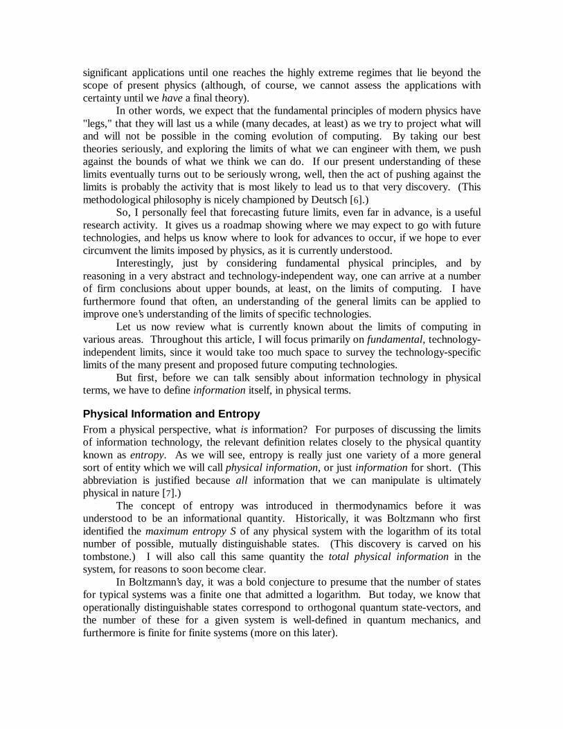
Figure 2. Physical Information, Entropy, and Known Information. Any physical system, when described only by constraints that upper-bound its spatial size and its total energy, still has only a finite number of mutually distinguishable states consistent with those constraints. The exact number N of states can be determined using quantum mechanics (with help from general relativity in extreme-gravity cases). We define the total physical information in a system as the logarithm of this number of states; it can be expressed equally well in units of bits or nats (a nat is just Boltzmann’s constant kB). In the example at right, we have a system of 3 two-state quantum spins, which has the 23=8 distinguishable states shown. It therefore contains a total of 3 bits = 2.08 kB of physical information.

Relative to some knowledge about the system’s actual state, the physical information can be divided into a part that is determined by that additional knowledge (known information), and a part that is not (entropy). In the example, suppose we happen to know (through preparation or measurement) that the system is not in any of the 4 states that are crossed out (i.e., has 0 amplitude in those states). In this case, the 1 bit (0.69 kB) of physical information that is associated with spin number 2 is then known information, whereas the other 2 bits (1.39 kB) of physical information in the system are entropy.

The available knowledge about the system can change over time. Known information becomes entropy when we forget or lose track of it, and bits of entropy can become known information if we measure them. However, the total physical information in a system is exactly conserved, unless the system’s size and/or energy changes over time (as in an expanding universe, or an open system).

1 2 3

Spin label

Informational Status

1 Entropy 2 Known

information 3 Entropy

Example: System with 3 two-state subsystems, such as quantum spins.

23=8 states

whose state is known (by a particular observer), and entropy be the information in the part that is unknown. The meaning of "known" can be clarified, by saying that a system A (the observer) knows the state of system B (the observed system) to the extent that some part of the state of A (e.g. some record or memory) is correlated with the state of B, and furthermore that the observer is able to access and interpret the implications of that record regarding the state of B.

To quantify things, the maximum known information or maximum entropy of any system is, as already stated, just the log of its possible number of distinguishable states. If we know nothing about the state, all the system’s physical information is entropy, from our point of view. But, as a result of preparing or interacting with a system, we may come to know (or learn) something more about its actual state, besides just that it is one of the N states that were originally considered "possible."

Suppose we learn that the system is in a particular subset of M<N states; only the states in that set are then possible, given our knowledge. Then, the entropy of the system, from our new point of view, is log M, whereas to someone without this knowledge, it is log N. For us, there is (log N) − (log M) = log(N/M) less entropy in the system. We say

1 2 3 4 5 6 7 8 9 10

0

0.2

0.4

0.6

0.8

1

Probability

State

NonUniform vs. Uniform Probability Distributions

1 2 3 4 5 6 7 8 9 10

0

20

40

60

80

OddsAgainst

(1 out of N)

State

Odds (Inverse Probability)

1 2 3 4 5 6 7 8 9 10

01234567

LogBase 2ofOdds

State

Log Odds (Information of Discovery)

1 2 3 4 5 6 7 8 9 10

0

0.1

0.2

0.3

0.4

0.5

Bits

State Index

Shannon Entropy (Expected Log Odds)

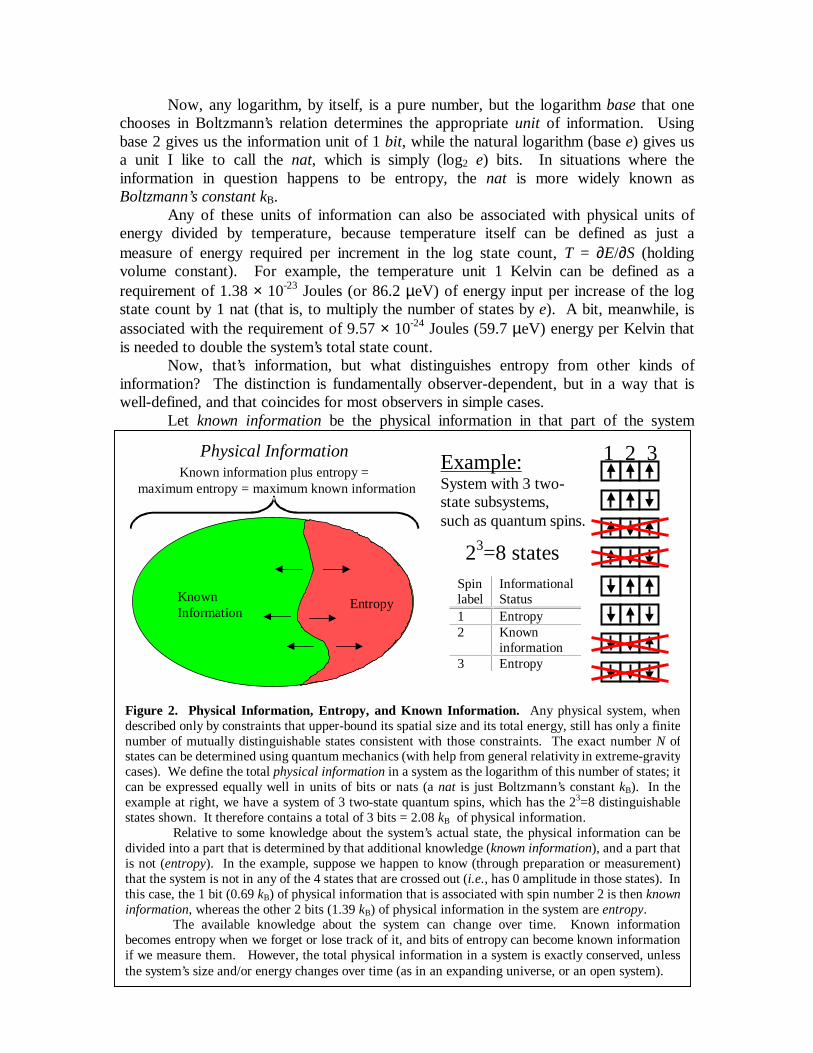
Figure 3. Shannon Entropy. The figure shows an example of Shannon’s generalization of Boltzmann entropy for a system having ten distinguishable states. The blue bars correspond to a specific nonuniform probability distribution over states, while the purple bars show the case with a uniform (Boltzmann) distribution. The upper-left chart shows the two probability distributions. Note that in the nonuniform distribution, we have a 50% probability for the state with index 4. The upper-right chart inverts the probability to get the odds against the state; state 4 is found in 1 case out of 2, whereas state 10 (for example) appears in 1 case out of 70. The logarithm of this "number of cases" (lower left) is the information gain if this state were actually encountered; in state 4 we gain 1 bit; in case 10, more than 6 bits (26=64). Weighting the information gain by the state probability gives the expected information gain. Because the logarithm function is concave-down, a uniform distribution minimizes the expected log-probability, maximizes its negative (the expected log-odds, or entropy), and minimizes theinformation (the expected log-probability, minus that of the uniform distribution).

we now know log(N/M) more information about the system, or in other words that log(N/M) more of the physical information that it contains is known information (from our point of view). The remaining log M amount of information, i.e., the physical information still unknown in the system, we call entropy.

So, you can see that if we know nothing about the system’s state, then it has entropy log N and we know log N − log N = 0 of the information in it. If we know the exact state of the system, then it has log 1 = 0 entropy, and we know the other log N − 0 = log N information in it. Anywhere in between, the system has some intermediate entropy, and we know some intermediate amount of its information.

Claude Shannon showed how the definition of entropy could be appropriately generalized to situations where our knowledge about the state x is expressed not as a subset of states, but as a probability distribution px over states. In that case the entropy is just ∑−=

xxx ppH .log The known information is then log N − H. Note that the

Boltzmann definition of entropy is just the special case of Shannon entropy where px happens to be a uniform distribution over all N states (see figure 3).

Anyway, regardless of our state of knowledge, note that the sum of the system’s entropy and its known information is always conserved. Known information and entropy are just two forms of the same fundamental quantity, somewhat analogously to kinetic and potential energy. Whether a system contains known information or entropy just depends on whether our state is correlated (in a known way) with the system’s state, or whether the states are independent. Information is just known entropy. Entropy is just unknown information.

Interestingly, physical information is apparently, like energy, a localized phenomenon. That is, it has a definite location in space, associated with the location of the subsystem whose state is in question. Even information about a distant object can be seen as just information in the state of a local object (e.g. a memory cell) whose state happens to have become correlated with the state of the distant object through a chain of interactions. Information can be viewed as always flowing locally through space, even in quantum systems [8]. In particular, quantum field theory, the global Hamiltonian of a system can always be constructed by combining Hamiltonians describing only local interactions.

Further, a system’s entropy may be converted to known information by measurement, and known information may be converted into entropy by forgetting (or erasure of information). But the sum of the two in a given system is always a constant, unless the maximum number of possible states in the system is itself changing, which may happen if the system’s changes in size, or if energy is added or removed. Actually, it turns out that in an expanding universe, the number of states (and thus the total physical information) is increasing, but in a small, local system with constant energy and volume, we will see that it is a constant. To say that entropy may be converted to known information through observation may at first sound like a contradiction of the second law of thermodynamics, that entropy always increases in closed systems. But remember, if we are measuring a system, then it isn’t completely closed, from an informational point of viewthe measurement requires an interaction that manipulates the state of the measurement apparatus in a way that depends on the state of the system. From a point of view that is external to the whole

measurement process, where we wrap a closed box around the whole process, the entropy, even if extracted from the original system through measurement, is still there (and still entropy) from this external point of view. (See figure 4.)

But, if entropy can be moved out of a system by measurement, then couldn’t you theoretically remove all the entropy from a cylinder of gas (for example) by repeated measurements, freezing it into a known state, and gaining its heat energy as work? Then, couldn’t you get more free energy, by allowing the cylinder to be warmed again by its surroundings while expanding against a piston, and repeat the experiment ad infinitum as a perpetual motion machine?

This question is exactly the famous Maxwell’s Demon "paradox" [9], which only seemed like a paradox (resisting all attempts at resolution) before Charles Bennett of IBM finally resolved it [10] with the realization that you have to keep track of where the extracted information goes. Sure, you can take entropy (and energy) out of a system, but you have to put the information somewhere, you can’t just "disappear" it. Wherever you put it, you will require energy to store it. You’ll need less energy, if you put the information in a lower-temperature system, but the resulting gain of work isn’t forbidden by thermodynamics, it’s just how any heat engine works! Now, Boltzmann developed his definition of entropy in the context of classical mechanics by making the seeming ad hoc assumption that even the seemingly-continuous states of classical mechanics were somehow discretized into a finite number that admitted a logarithm. However, this notion was later vindicated, when Max Planck and the entire subsequent development of quantum mechanics showed that the world was discretized, at least in the relevant respects. The entire classical understanding of the relations between entropy, energy, temperature, etc., remained essentially valid, forming the whole field of quantum statistical mechanics, a cornerstone of modern physics. Only the definition of entropy had to be further generalized, since partially-known states in quantum mechanics are described not by probability distributions, but by a generalization of a probability distribution called a mixed state or density operator, which can be represented (in finite cases) by density matrices. However, entropy can still be defined for these more complex objects in a way that remains perfectly consistent with the more

0/1 0 AA

B

0/1 0/1 A B

C

C

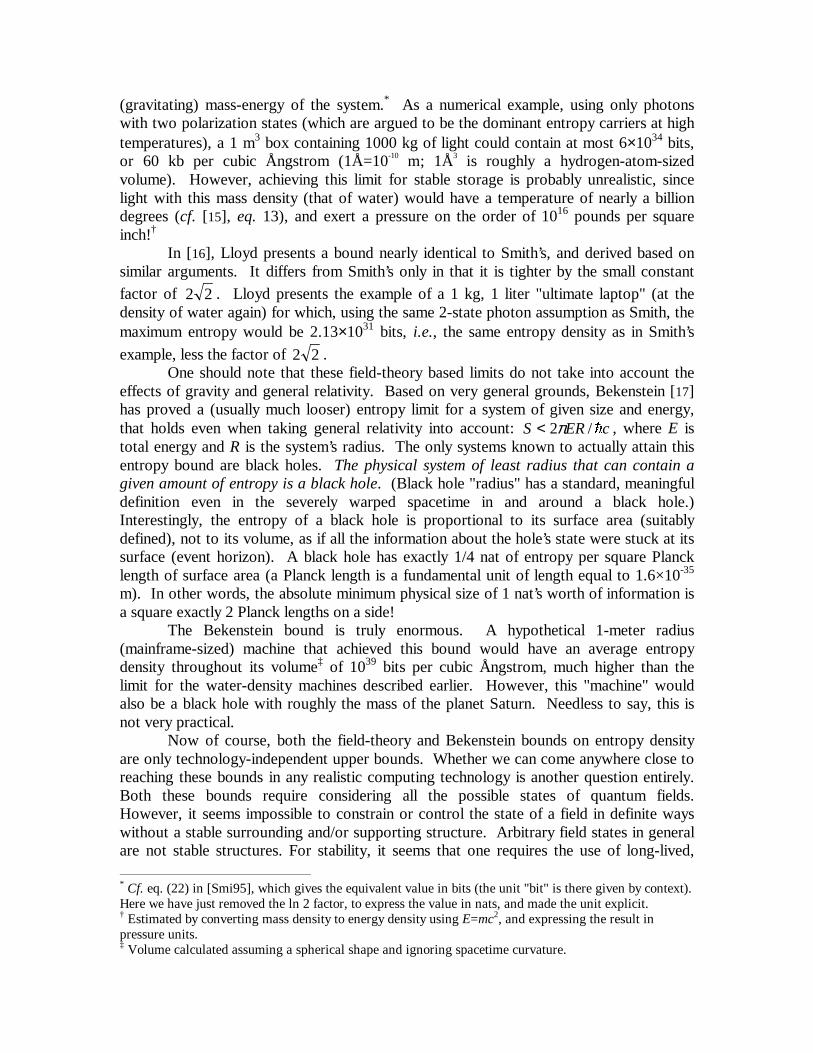
Figure 4. Entropy & measurement. Suppose system B, which contains 1 bit of entropy (two possible states, labeled 0 and 1), is measured by system A (arrow). Now, system A is correlated with B, and B’s physical information is now known information, from A’s point of view. But from the point of view of an outside observer C who does not have access to A’s record, the combined system still has 1 bit of entropy, since it could be either in state (A=0,B=0) or state (A=1,B=1). Since physics is invertible, the number of possible states of the whole system can’t decrease from the point of view of an outsider who isn’t measuring its state. But it can increase, for example, if C loses track of the interactions taking place between A and B, in which case all 4 joint states of the AB system might become possibilities from C’s point of view.

restricted cases addressed by Boltzmann and Shannon (see fig. 5). The study of the dynamic evolution of mixed states in quantum mechanics leads to a fairly complete understanding of how the irreversible behavior described by the second law arises out of reversible microphysics, and how the quantum world appears classical at large scales. Basically, it all comes down to information and entropy.

Quantum states, obeying Schrödinger’s wave equation, tend to disperse outside of any localized region of state space to which they are initially confined (except for the case of energy eigenstates, such as electron orbitals, which are stable). Systems evolve deterministically, but when you project their quantum state down to a classical probability distribution, you see that an initial sharp probability distribution tends to spread out, increasing the Shannon entropy of the state over time. The state, looked at from the right perspective or basis, is still as definite as it was, but as a matter of practice, we generally lose track of its detailed evolution; so the known information the system had (from our point of view) effectively becomes entropy. The new field of quantum computing, on the other hand (cf. [11]), is all about isolating a system and maintaining enough control over its evolution so that we can keep track of its exact quantum state as it deterministically changes. The physical information in a quantum computer is therefore known information, not true entropy. However, most systems are not so well isolated; they leak state information to the outside world; the environment "measures" their state, as it were. The environment becomes then correlated with the system’s state, and so copies of the system’s state information become mixed up with and redundantly spread out over arbitrarily large-scale surrounding systems. This precludes any control over the precise evolution of that state information, and so we fail to be able to elicit any quantum interference effects, which can only appear in well-defined deterministic situations, where multiple dynamic trajectories are made to converge onto a single state of the whole system.

The precise way in which even gradual measurement by the environment eats away at quantum coherences, effectively devolving a pure quantum state into a (higher-entropy) mixed state, and making the large-scale world appear to have an objective but

von Neumann entropy:

n

H

iiiii

iiiii

ln

ln

’ln’

’ln’Tr

lnTr)(

≤

−≤

−=−=−=

∑∑

ρρ

ρρρρρρρ

Figure 5. Density matrix representation of probabilistic mixtures of quantum states. The rows and columns of ρ are indexed by the system’s distinguishable states (in any basis). Each diagonal element ρii just gives the probability of basis state i. The off-diagonal elements ρij, i≠j are complex numbers that specify quantum coherences between the basis states. Any density matrix ρ has a unique basis such that when ρ is re-expressed in that basis, the resulting matrix ρ’ is diagonal, and represents a classical mixture of ≤n basis states. The basis-independent von Neumann entropy of a mixed state is given by H = −Tr ρ ln ρ (where ln represents a matrix logarithm, defined as the inverse of matrix exponential, which is defined by a Taylor-series expansion of eM). This quantity is exactly the same as the Shannon entropy (in nat units) of the probability distribution specified along the diagonal of the diagonalized density matrix ρ’. The von Neumann entropy of a (not necessarily diagonal) density matrix ρ is always less than or equal to the Shannon entropy of ρ’s own diagonal, which is in turn always less than or equal to the Boltzmann entropy, ln n.

=

nnnn

n

n

ρρρ

ρρρρρρ

ρ

�

����

�

�

21

22221

11211

⇒

=

nn’00

0’0

00’

’ 22

11

ρ

ρρ

ρ

�

����

�

�

nondeterministically determined classical state, is by now well understood by those who have studied this problem, particularly Zurek [12]. Straightforward, deterministic quantum theory actually requires no modifications (such as ad hoc "wavefunction collapse") in order to explain classical macro-behavior perfectly well as an emergent phenomenon, an insight first elucidated by Everett [13]. Unfortunately, these important facts are not as widely known or understood as they should be, and as a result, this elegant theory is still undeservedly controversial in many circles, where it is still imagined to conflict with macroscopic experience.

Information Storage Limits Now that we know what information physically is (more or less), let’s talk about some of the limits that can be placed on it, based on known physics. An arbitrary quantum wavefunction, as an abstract mathematical entity, in general could require infinite information to describe precisely, because in principle there is an uncountable set of possible wavefunctions. (Note, however, that there are only countably many finite descriptions, or computable wavefunctions.) But remember, the key definition for physical information, ever since Boltzmann, is not the number of states that might mathematically exist, but rather the number of operationally distinguishable states. Quantum mechanics gives distinguishability a precise meaning: Namely, two states are 100% distinguishable if and only if (considered as complex vectors) they are orthogonal.

A basic result in quantum statistical mechanics is that the total number of orthogonal states for a system consisting of a constant number of non-interacting particles, having relative positions and momenta, is roughly given by the numerical volume of the particles’ joint configuration space or phase space (whatever its shape), when expressed in length and momentum units chosen so that Planck’s constant h (which has units of length times momentum) is equal to 1 (cf. sec. 2.D of [14]). Therefore, so long as the number of particles is finite, and the volume of space occupied by the particles is bounded, and their total energy is bounded, then even though (classically) the number of point particle states is uncountably infinite, and even though the number of possible quantum wavefunctions is also uncountably infinite, the amount of information in the system is finite! Now, this model of a constant number of non-interacting particles is a bit unrealistic, since in quantum field theory (the relativistic version of quantum mechanics), particle number is not constant; particles can split (radiation) and merge (absorption). To refine the model one has to talk about possible field states with varying numbers of particles. However, this still turns out not to fundamentally change the conclusion of finite information for any system of bounded size and energy. In independent papers, Warren Smith of NEC [15] and Seth Lloyd of MIT [16] have given an excellent description of the quantitative relationships involved.

In his paper, Smith argues for an upper bound to entropy S per unit volume V of

nat603

16

2

4/3

4/1

4/1

⋅

⋅

=

V

Mcq

V

S �π,

where q is the number of distinct particle types (including different quantum states of a given particle type), c is the speed of light, � is Planck’s constant, and M is the total

(gravitating) mass-energy of the system.* As a numerical example, using only photons with two polarization states (which are argued to be the dominant entropy carriers at high temperatures), a 1 m3 box containing 1000 kg of light could contain at most 6×1034 bits, or 60 kb per cubic Ångstrom (1Å=10-10 m; 1Å3 is roughly a hydrogen-atom-sized volume). However, achieving this limit for stable storage is probably unrealistic, since light with this mass density (that of water) would have a temperature of nearly a billion degrees (cf. [15], eq. 13), and exert a pressure on the order of 1016 pounds per square inch!†

In [16], Lloyd presents a bound nearly identical to Smith’s, and derived based on similar arguments. It differs from Smith’s only in that it is tighter by the small constant

factor of 22 . Lloyd presents the example of a 1 kg, 1 liter "ultimate laptop" (at the density of water again) for which, using the same 2-state photon assumption as Smith, the maximum entropy would be 2.13×1031 bits, i.e., the same entropy density as in Smith’s

example, less the factor of 22 . One should note that these field-theory based limits do not take into account the

effects of gravity and general relativity. Based on very general grounds, Bekenstein [17] has proved a (usually much looser) entropy limit for a system of given size and energy, that holds even when taking general relativity into account: cERS �/2π< , where E is total energy and R is the system’s radius. The only systems known to actually attain this entropy bound are black holes. The physical system of least radius that can contain a given amount of entropy is a black hole. (Black hole "radius" has a standard, meaningful definition even in the severely warped spacetime in and around a black hole.) Interestingly, the entropy of a black hole is proportional to its surface area (suitably defined), not to its volume, as if all the information about the hole’s state were stuck at its surface (event horizon). A black hole has exactly 1/4 nat of entropy per square Planck length of surface area (a Planck length is a fundamental unit of length equal to 1.6×10-35 m). In other words, the absolute minimum physical size of 1 nat’s worth of information is a square exactly 2 Planck lengths on a side!

The Bekenstein bound is truly enormous. A hypothetical 1-meter radius (mainframe-sized) machine that achieved this bound would have an average entropy density throughout its volume‡ of 1039 bits per cubic Ångstrom, much higher than the limit for the water-density machines described earlier. However, this "machine" would also be a black hole with roughly the mass of the planet Saturn. Needless to say, this is not very practical. Now of course, both the field-theory and Bekenstein bounds on entropy density are only technology-independent upper bounds. Whether we can come anywhere close to reaching these bounds in any realistic computing technology is another question entirely. Both these bounds require considering all the possible states of quantum fields. However, it seems impossible to constrain or control the state of a field in definite ways without a stable surrounding and/or supporting structure. Arbitrary field states in general are not stable structures. For stability, it seems that one requires the use of long-lived, * Cf. eq. (22) in [Smi95], which gives the equivalent value in bits (the unit "bit" is there given by context). Here we have just removed the ln 2 factor, to express the value in nats, and made the unit explicit. † Estimated by converting mass density to energy density using E=mc2, and expressing the result in pressure units. ‡ Volume calculated assuming a spherical shape and ignoring spacetime curvature.

bound particle states, such as one finds in molecules, atoms and nuclei. This leads us to our next logical question:

How many bits can you store in an atom? Nuclei may have an overall spin orientation, which is encoded using a state-vector space of only dimensionality 2, so the spin only holds 1 bit of information. Aside from its spin variability, at normal temperatures a given nucleus is normally frozen into its quantum ground state. It can only contain additional information if it is excited to higher energy levels. But, excited nuclei are not stable—they are radioactive and decay rapidly, emitting high-energy, damaging particles. Not too nice for consumer safety! Electron configuration is another possibility. Outer-shell electrons may have spin variability, as well as excited states that, although still unstable, at least do not present a radiation hazard. Further, there may be many ionization states for a given atom that may be reasonably stable in a sufficiently well-isolated environment. This presents another few potential bits. The choice of nuclear species in the atom in question presents another opportunity for variability. However, there are only a few hundred reasonably stable isotopes, so at best (even if you have a storage location that can hold any type of atom) this only gives you at most an additional 8 bits or so. An atom in a solid is in a potential energy well (relative to its neighbors) and generally has 6 restricted degrees of freedom, three of position and three of momentum. At normal temperatures, each one of these contributes kB/2 to its heat capacity, which contributes an equivalent amount of entropy for each factor of e increase in temperature beyond the regime where the excited states become accessible. So this gives us a few more bits per atom, encoded in these vibrational states. However, phonons (the quantum "particles" of mechanical vibration) can easily dissipate out into any mechanical supporting structure, so they do not represent stable storage.

Of course, an arbitrarily large number of bits could be encoded in an atom's position and momentum along unrestricted degrees of freedom, i.e., in infinitely large open spaces. However, given bounded spaces and energies, the entropy is still limited by the classical limit of log phase-space-volume (mentioned earlier). Since entropy per atom grows with only log volume, entropy density (per volume) actually shrinks with increasing volume. So, spreading atoms out, though it increases entropy per atom (by some small number of bits) does not increase entropy density. If we are interested in maximizing information density using atoms, then we should stick with dense, solid-state materials (which also have the advantage of stability).

For example, a rough estimate I performed of the entropy density in pure copper, based on standard CRC tables of empirically-derived thermochemical data, suggests that (at atmospheric pressures) the actual entropy density falls in the rather narrow range of only about 0.5 to 1.5 bits per cubic Ångstrom, over a wide range of temperatures, from room temperature up to just below the metal's boiling point.* Entropy densities in a variety of other pure elemental materials are also near this level, though copper had the highest entropy density of the materials I studied. The entropy density would be expected to be somewhat greater for mixtures of elements, but not by much.

* This estimate was arrived at by integrating the approximate heat capacity, divided by temperature, over the temperature range, and adding in the change of entropy during the solid-liquid transition.

One can try to further increase entropy densities by applying high pressures. At the moment, it is unclear what may be the ultimate limits to pressures achievable in stable structures. The only clear limit I know of is the pressure at the core of neutron star just below the critical mass (~3.2 suns) for black hole collapse (~1030 atmospheres*). But of course, stellar-scale engineering is, at best, only a very long-term prospect.

Based on all this, I would be quite surprised if an information density greater than, say, ~10 bits per cubic Ångstrom could be achieved for stable, retrievable storage of digital information anytime within, say, the next 100 years.

Note, however, that even at an information density of only 1 bit/Å3 (which the Moore's Law trend would have us reach in only 40 years or so), a convenient 1 cm3 (sugar-cube size) lump of material could theoretically hold 1024 bits of information. This quantity (or actually the slightly greater quantity 280 bits) is known, in obscure jargon†, as 1 yottabit or 1 Yb. In more familiar units, it is ~100 billion terabytes, much greater than the total digital storage in the entire world today.

Minimum Energy for Information Storage One of the most important raw resources involved in computing, besides time and

space and manufacturing cost, is energy. When we talk about "using up energy," we really mean converting free energy into (low-temperature, or degraded) heat energy, since energy itself is conserved. Free energy can be loosely defined as that part of the accessible energy that we could potentially organize into a structured configuration, work (such as a directed energy of motion) that would accomplish some desired transformation of some system of interest.‡

These concepts relate to information, as follows. A given chunk of energy can be thought of as carrying an associated chunk of information describing the state of that energy. Heat can be broadly defined as any energy all of whose information happens to be entropy. In other words, its state is completely unknown. For a system with entropy S at temperature T, we can even define its internal heat as ST.

However, part of the heat in any high-temperature system is also free energy, because it can be converted to work, by extracting its entropy into a smaller amount of heat that is expelled into a lower-temperature system—this is just what any heat engine does. Temperature, as we saw earlier, is just the slope of the energy vs. information curve for a given (open) system whose total energy and physical information are (for whatever reason) subject to change.

If a system has entropy S and the coolest available reservoir large enough to hold this entropy has temperature TC, then we know that an amount STC of the energy in the system is permanently committed to storing this entropy. We can call this the spent energy. After excluding the entropy and its associated spent energy from the system, the rest of the system's accessible energy will be in a known state—but, this does not necessarily mean a desired state. We may need to manipulate the system's information to get it into the form we want.

* The equivalent pressure corresponding to several times the nuclear saturation density of 2.7×1014 g/cm3. † The "yotta" prefix was adopted in 1990 by the 19th Conférence Générale des Poids et Mesures (CGPM), cf. http://www.bipm.fr/enus/3_SI/si-prefixes.html. ‡ More precisely defined measures of free energy include Gibbs free energy and Helmholtz free energy, but their particular definitions are not required for our present purposes.

What are the constraints on manipulations that we can do? One major constraint comes from the fact that physics is reversible, meaning that in a closed system it transforms one state to another over time in a mathematically invertible way. Another way of saying this is that it is deterministic looking backwards in time. This follows from the unitary nature of the time-evolution operator in quantum mechanics, but is also a feature of any mechanics that admits of a Hamiltonian description.*

Reversibility can be seen as directly implying the second law of thermodynamics: If a bit of entropy in a closed, unmeasured system were to disappear (be transformed to a known state), this would not be reversible, because multiple possible prior states would be mapped to the same resulting state. Such a transformation would have no inverse. In contrast, appearance of entropy only requires the "knower" to forget or lose track of the system’s state, which is easy to do.†

Now, let us return to the topic of this section: the energy required for information storage. What do we mean by information storage? Namely, that "we" (namely, the entity in question, whether a human or a computer) have learned some piece of information— either via a measurement (input operation), or by some internal computation— and we wish to record a copy of it, temporarily or permanently, in some accessible system (a "storage location") in such a way that we can use it later. That is, we wish the system's state to become correlated with the information obtained.

The question is: What happens to the physical information that was already in the storage location to be correlated with the new information? Due to the reversibility of physics, it cannot simply disappear and be replaced by the known information. There are only three possibilities:

(1) If the storage location is in a known state, that means it is correlated to or

redundant with some other system that we can access (namely, wherever our knowledge resides), and further that we know the form of this correlation. As a result, it may be possible to reversibly return the storage location to some standard, "empty" state— for example, by the reverse of the operation that created the correlation to begin with, or, there are sometimes other methods. We call this uncomputing the information.

Once its informational content has been uncomputed, the system is then in the empty state and can be reused— a reversible tranformation can now take it to a new state that explicitly represents the particular information that we wish to store. To the extent that we can avoid creating any new entropy during this entire reversible process, we can avoid spending any energy. (Recall the definition of spent energy from above.) The reversible reuse of storage for

* Note that reversibility is not the same thing as time symmetry. Although most physical laws are time-symmetric, particle physics has shown that one must also negate all electrical charges and replace all spatial configurations with their mirror-images in order to obtain exactly identical laws. Particle physics is now thought to obey only "charge-parity-time" or CPT symmetry. However, regardless of the precise symmetry, all the currently tenable theories are (apart from the required sign changes) unchanged in overall form with respect to time reversals, and so they remain reversible; that is, reverse-deterministic. † There is a small subtlety here— is information considered known if it is merely deducible from known information? The problem is that deductions can be arbitrarily difficult. Information that is infeasible to deduce is, at least, effectively unknown, and thus effectively entropy, though note that it would "become" non-entropy if one went through the time and trouble to deduce it.

multiple computations that produce useful results was first shown theoretically possible by Charles Bennett of IBM [18], although earlier work by Landauer [19] and Lecerf [20] came close to making this discovery.

(2) If the storage location is in an unknown state (contains entropy), then the best

that we can do is to reversibly move the entropy S away to some system at temperature T, which requires that, at least, the corresponding energy ST must go along with it. For example, if S = 1 bit (kB ln 2), then at least kBT ln 2 energy must be dissipated. Landauer was the first to detail the argument about the minimum energy expenditure in this case (1961, [19]).* *21

(3) This third possibility is rarely considered. The existing information in the

storage location can be reversibly transformed in a way that depends on the new information, but also on the old. If the contents of the storage location are measured both before and after such transformations, then the correlations between the states of the storage location at different times can potentially be harnessed to effectively utilize the new "stored" information, despite the fact that the old information remains present (though possibly in altered form). However, the usefulness of this particular technique may be quite limited.†

An interesting fact about present-day commercial computer technology is that every act of information storage (e.g. every bit-operation performed by each of the millions of logic gates in a modern CPU every nanosecond) treats the previous contents of the storage location as being unknown, and uses method (2), and furthermore with many orders of magnitude of added energy-inefficiencies on top of this. However, there is now a new research field (small, but growing) of reversible computing, which is concerned with investigating the alternative of using technique (1) instead, and of engineering systems that approach the theoretical possibility of zero dissipation as closely as possible.

It seems that real technologies can indeed approach these predictions, as indicated by Likarev’s analysis of his reversible superconducting "parametric quantron" [22], as well as by the adiabatic‡ CMOS circuits that have been a popular topic of investigation and experimentation (for myself and co-workers, among others) in recent years (cf. [23,24,25,26]).

Our group at MIT designed and built several adiabatic processors (see fig. 6), demonstrating that there is nothing inherently impossible or even especially difficult about building real computer architectures based on reversible logic. These techniques

* Von Neumann had discussed but not proven this limit in an earlier (1949) lecture, published posthumously in 1963 [21]. † The only nontrivial example of this trick that I know of is in a group-theoretic circuit construction by Coppersmith and Grossman [CG75] showing that arbitrary Boolean functions of n-bit inputs can (surprisingly) be reversibly computed "in place" using the input locations plus at most 1 extra bit of storage, which need not initially be empty. Unfortunately, in that example, the technique does not lead to a practical (time-efficient) algorithm. ‡ Adiabatic processes are ones that asymptotically approach thermodynamic reversibility at low speeds, although we should note that no highly-structured system can be fully adiabatic, because it is always subject to some nonzero background rate of decay towards a less structured equilibrium ensemble.

may even soon lead to cost-efficiency benefits in electronics applications that demand extremely low power consumption.

However, some interesting fundamental research problems remain to be solved before the practicality of these kinds of approaches for breaching sub-kBT energy levels can be firmly established. Let us elaborate.

Some Open Problems in Reversible Computing First, there is an open research issue of how to provide appropriate synchronization in a scalable, parallel reversible processor. Let us explain.

In order to make rapid forward progress through the computation, the machine state needs to evolve nearly ballistically (that is, dominated by its forward momentum, rather than by a random walk) along its trajectory in configuration space. Zurek, however, showed that a certain ballistic asynchronous (clockless) reversible processor would be disastrous under classical physics, since small misalignments in the arrival times of different ballistically-propagating signals would throw off the interactions and lead to chaos [27] (specificially, in Ed Fredkin’s original "billiard ball model" [28] of ballistic reversible computing).* However, Zurek’s paper also showed that quantum

* Smith [Smi99] later described a classical reversible machine that also avoided instability, but it was not hardware-efficient (each location could be used only once), so did not really demonstrate sub-kT dissipation per operation if the energy cost of building the hardware is taken into account.

Figure 6. Reversible chips designed at MIT, 1996-99. As graduate students in Tom Knight’s group, my co-workers (Josie Ammer, Nicole Love, Scott Rixner, Carlin Vieri) and I designed, outsource-fabricated and tested these four proof-of-concept reversible chips, using the "Split-Level Charge Recovery Logic" (SCRL) adiabatic CMOS logic family that had been introduced by Knight and Younis in 1993-94 [23]. Cadence design tools and a 0.5-µm process provided by MOSIS were used. TICK was a benchmark for comparison purposes, an 8-bit, non-adiabatic implementation of a reversible instruction set architecture, while PENDULUM was a 12-bit fully-adiabatic implementation with a similar ISA, but designed to achieve much lower power [25]. Before PENDULUM, we built the much simpler FLATTOP, a fully-adiabatic programmable array of 400 simple 1-bit processing elements; arrays of these chips could in principle be programmed to simulate arbitrary reversible circuits in a scalable way [24,26]. XRAM

was a small fully-adiabatic static RAM chip.

systems need not suffer from such instabilities, and that their errors could in principle be corrected with relatively little dissipation.

Zurek’s insight was taken further by Feynman [29] who constructed a detailed quantum model of a serial (one operation at a time) reversible computer that required no global synchronization; only local, self-timed interactions. Margolus [30] extended this technique to a parallel model, but was able to prove a steady rate of computation for only 1 dimension of parallelism, that is, for architectures with at most order N1 active locations accessible within time N. For improved spacetime efficiency of algorithms, we would prefer that order N3 elements be accessible (the maximum possible in flat 3-dimensional space). Whether Margolus’ technique, or any other, will work for self-synchronizing reversible computations with scalability in more than 1 dimension remains to be seen.

If the self-timed approach does not work out, then apparently an accurate, synchronous global timing signal will need to be provided in order to keep the logic signals in the machine aligned in time. In fact, all reversible machine implementations proposed so far (including the quantum computers) depend on this approach, as do most irreversible commercial processors (although irreversible self-timed chips have already been commercially demonstrated [31]). One expects it to be theoretically possible to construct a resonant clock generator that recycles energy with arbitrarily high efficiency.

However, no one has yet proposed a specific mechanism for such a clock generator that is accompanied by a sufficiently detailed scaling analysis (preferably backed up by experiment, or at least a detailed simulation) to establish that the entire system (including the clock generator) can clearly and obviously be scaled to sub-kT dissipation levels per logic operation that it drives, while also scaling up cost-effectively to arbitrarily large numbers of processing elements working together in parallel, preferably in 3-dimensional arrays. Indeed, some early indications suggest that there may be quantum limits that imply that global timing signals ultimately will not scale properly, due to quantum uncertainty [32].

Merkle and Drexler’s helical logic proposal [33], involving a cylindrical spindle of wires rotating slowly in an electrostatic field, is one example of an implementation concept which might have potential, but its engineering details have probably not been worked out with quite enough thoroughness yet to convince everyone of its feasibility.

As an example of a skeptical viewpoint, Smith [34] conjectures a "no free lunch" principle, that any physical mechanism offering sub-kT computational operations must necessarily suffer from fatal asymptotic space-time overheads, such as an inability to reuse hardware. Another notable expression of skepticism about reversible computing is that found in Mead and Conway’s well-known VLSI textbook [35].

However, despite these doubts, and despite the lack of any experimentally validated implementation as a counter-example, none of the skeptics have given any rigorous proof, or even any very convincing argument (in my opinion) why a hardware-efficient and scalable sub-kBT logic technology must be fundamentally impossible for any technology, as opposed to merely being unattained by various specific mechanisms.

So, to the best of my knowledge, at the moment it is still technically an open question whether computing with arbitrarily little entropy generation per operation (with hardware reuse, and scalable 3-D parallelism) is truly permitted, or not. Finding the definitive answer to this crucial question (whether it be yes or no) is a key goal of my own research at the moment.

Interestingly, even if efficient physically-reversible computing turns out to be permitted in principle, it is probably not quite as good as it sounds at first for all applications, because of the algorithmic overheads that appear to be associated with reversible computing in general [36]. Definitively proving lower bounds on the magnitude of these overheads is another fundamental open problem.

Furthermore, in any fixed device technology having a minimum rate of energy leakage, one can show that there will be a maximum degree of reversibility that can be beneficial, so that any given technology’s dissipation per operation, even if much less than kBT, is not arbitrarily smaller. Accurately characterizing the cost-efficiency tradeoffs in this situation is another open problem that is less fundamental, but important for near-term applications.

So, to wrap up our discussion of information storage, what is the minimum energy required to "store a bit of information?" That depends. If all that is needed is to reversibly change the state of a storage location from one definite state to another, then there is no lower limit, apparently [18,10]. However, if the storage location already contains entropy, or just some information that we wish to forget, then we have to move this existing information out of the system to the unlimited space in the external world, which costs kBT ln 2 free energy, where T is the temperature at the point where we finally

Trend of minimum transistor switching energy

1

10

100

1000

10000

100000

1000000

1995 2005 2015 2025 2035

Year of First Product Shipment

Min

tra

nsi

sto

r sw

itch

ing

en

erg

y, k

Ts

High

Low

trend

Figure 7: Trendline of minimum ½CV2 transistor switching energy. Values were calculated using the goals for high-performance and low-power processors in the 1999 International Technology Roadmap for Semiconductors [3]. Energy is expressed as a multiple of room-temperature kT, which also is the number of nats of information associated with that energy. If the trend is followed, thermal noise will begin to become significant in the 2030s, when transistor energies approach small multiples of kT. Shortly after 2035 (if not sooner) this trend will be forced to begin leveling off, since a bit of information requires at least 0.69 kT to carry it [37]. However, if reversible operations are used, the order-kT bit energies need not be dissipated [19,18], and so the dissipation per reversible bit manipulation might continue decreasing along this curve a while longer.

thermalize (lose control of) the information. We cannot simply wish away the information, somehow compressing the system’s number of possible states, because physics is reversible (as discussed earlier), and phase space is incompressible (Liouville’s theorem). The true entropy (von Neumann entropy) of a mixed quantum state of an unobserved, closed system does not decrease as the system evolves unitarily, though it can increase, insofar as we lose track of the system’s detailed evolution. It is interesting to note that current technology is a bit closer to approaching the fundamental limits on energy dissipation for information storage, compared to how far we would have to go to achieve the limits on information density. Current trends would have us reach the limit of kBT ln 2 (i.e., 1 bit of physical information displaced per bit of digital information irreversibly stored) in only about 35 years (see figure 7).37At this time (if not sooner), the performance per unit power of ordinary irreversible computing (which does an irreversible storage operation with every logic-gate operation) will start to level off, at a maximum level of at most 3.5 × 1022 irreversible bit-operations per second in a 100 W computer that disposes displaced entropy into a room-temperature (300 K) thermal reservoir. This rate is about a million times higher than the maximum rate of bit operations in the ~30-million-gate, 1 GHz processors in use today. Any possible further improvements in performance-per-power beyond this point would require reversible computing.

Communication Limits Communication is important in computing because it constrains the performance of many parallel algorithms. In his well-known work [38] spawning the field of information theory, Claude Shannon derived the maximum information-carrying capacity of a single wave-based communications channel (of given frequency-band width) in the presence of noise. Shannon’s limits are widely studied, and are fairly closely approached by the coding schemes used in state-of-the-art wave-based communications today. However, when considering the ultimate physical limits relevant to computation, we need to go a bit beyond the scope of Shannon’s paradigm. We want to know not only the capacity of a single channel, but also the maximum bandwidth for communication using any possible number of channels, given only area and power constraints. Interestingly, the limits from the previous section, on information storage density and energy, directly apply to this. Consider: The difference between information storage and information communication is, most fundamentally, only a difference in one’s inertial frame of reference. Communication from point A to point B is ultimately just bit transportation, i.e. a form of "storage" but in a state of relative motion. And likewise, storage is just "communication" across zero distance (but through time). So, if one has a limit on information density ρ, and a limit on information propagation velocity v, then this immediately gives a limit of ρv on information flux density (or just flux for short), that is, bits per unit time per unit area in communications. Of course, we always have a limit on propagation velocity, namely the speed of light c, and so each of the information density limits mentioned earlier directly implies a limit on flux density (though relativistic corrections are needed for speeds approaching c). One can then derive a maximum information "bandwidth" per unit area (i.e., information flux), as a function of per-area power density (energy flux).

For example, Smith [15] shows that the maximum entropy flux FS using photons,

given energy flux FE, is 4/3E

4/1SBS 3

4FF σ≤ , where σSB is the Stefan-Boltzmann constant

π2kB4/60c2 � 3. So, for example, a 10-cm square wireless tablet transmitting

electromagnetically at a 1 W power level (from one side) could never communicate at a bit rate of more than 6.8 × 1020 bits per second, no matter what distribution of frequencies or coding scheme is used, even in the complete absence of noice.

This limit sounds very high at first, but consider that the corresponding bit rate per square nanometer is only 68 kbps. For communication among neighboring devices across a cross-section of a computer having densely-packed nano-scale components, one would like a much higher bandwidth density, perhaps on the order of 1011 bps/nm2, to keep up with the ~100 GHz expected rate of bit-operations in a nanometer-size electronic component that is 1/100 the size of today’s ~0.1 µm transistors. This ~106× higher information flux would require a (106)4/3 = 108× higher power density (from Smith’s law), that is, on the order of 1 MW/cm2! The equivalent temperature (that of blackbody radiation with this power density) is about 14,000 K.* (Any other spectrum would require even higher power levels, since the equilibrium spectrum by definition has the maximum entropy.) This seems too high to be practical (the computer would melt), so it seems that we can rule out light as a practical medium for dense interconnects at the nano-scale, at least until we find some way to build stable structures at such temperatures.† In contrast, notice that if a bit were encoded in more compact particles (atomic or electronic states), rather than in electromagnetic field modes, then, given a plausible information density of 1 bit per cubic nanometer, our desired bit-rate of 1011 bps/nm could be achieved using a quite reasonable velocity (of atoms or electrons) of only 100 m/s. Another interesting consideration is the minimum energy dissipation (as opposed to energy transfer) required for communications. As we saw earlier, one can look at a communication channel as the same thing as a storage element, but looked at from a different relativistic "angle," so to speak. If the channel’s input bit is in a definite state, then to swap it with the desired information takes no energy [39]. The channel does its thing (ideally, ballistically transporting the energy being communicated, over a definite time span), and the information is then swapped out at the other end— although the receiver needs an empty place to store it. However, if the receiver's storage location is already occupied with a bit that's in the way of your new bit, and that you can't uncompute, then you have to pay the energetic price to dispose of the old bit.

Computation Rate Limits So far we have focused only on limits on information storage and communication. But what about computation itself? What minimum price, in terms of raw physical resources, must we pay for computational operations? Earlier, we discussed the thermodynamic limit on computational performance of irreversible computations as a function of their power dissipation, due to the need for * Obtained by dividing the power flux by c to convert it to energy density, then solving Smith’s eq. 13 (energy density of blackbody radiation) for T. † Unless a way is found to increase the entropy density of EM fields beyond this bound. This might be done if, for example, EM waves could be confined to channels much smaller than their wavelength.

removal of unwanted (garbage) information. However, this limit may not apply to reversible computations. Are there other performance limits that will apply to any type of computation, reversible or not? Interestingly, yes: Basic quantum theory can be used to derive a maximum rate at which transitions (such as bit-flips) between distinguishable states can take place [40,16]. One form of this upper bound depends only on the total energy E in the system, and is given by 4E/h, where h=2π � is the unreduced Planck’s constant.

At first, this seems like an absurdly high bound, since the total energy presumably includes the rest-mass-energy of the system, which, if the system contains massive particles, is a substantial amount of energy. For example, Lloyd’s 1-kg "ultimate laptop" has a mass-energy of 9×1016 Joules, and so its maximum rate of operation comes out to be 5×1050 state-changes per second!

However, if the system’s whole mass-energy is not actively involved in the computation, then presumably it is only that portion of the mass-energy that is involved that is relevant in this bound. This gives a much more reasonable level. For example, a hypothetical single-electron device technology in which electrons operate at 1 eV above their ground state could perform state-transitions at a maximum rate of about 1 PHz (1015 Hz) per device. Interestingly, as with the speed limit due to energy dissipation, this is only about a factor of a million beyond where we are today.

Conclusion All computer users, including computational scientists & engineers, naturally hope that the trend of increasing affordability of computing power will take us as far as possible. Where the limits of computing lie is obviously an important; indeed, some have suggested it may even have a bearing on the long-term fate of life in the universe!41 However, our best available knowledge of physics strongly indicates that some ultimate limits do exist, and give us, at least, loose upper bounds on what might be achieved.

Interestingly, one of the most imminent of the fundamental limits appears to be the limit on the energy dissipation of irreversible computation, but this particular limit may possibly be circumvented through the use of reversible computing techniques. Although reversible computing has made impressive progress, whether this "fix" can ultimately work out in a scalable and cost-efficient way remains to this day an open question, one that is the subject of active research by myself and others.

As part of my future work, I am planning to apply methods of computational physics to model and simulate various candidate reversible computing systems, taking all the relevant physical considerations into account, until either a complete and detailed proof-of-concept model of a realistic, cost-efficient, and scalable sub-kBT computing system is developed, or it becomes clear how to construct a rigorous and general proof that no mechanism having all the desired properties can physically exist.

In any event, I hope that the present article will help to inspire scientists & engineers in many fields to devote increased attention to finding ways to meet the incredible challenges facing the future of computing, as it approaches the many limits found at the atomic scale. These limits are now close enough to fall within the career horizons of people starting out today: For example, given present rates of improvement, computing will hit the kBT thermodynamic brick wall before today’s 30-year-old Ph.D. graduates will retire. Although computing does appear to be nearing various hard

physical limits, the race to get as far as possible within those limits promises many exciting research opportunities in many areas of the physical and computer sciences, as we develop these new machines.

But, even if someday we figure out how to optimally harness all of the raw computational power of physics itself, we can be sure that our ultimate "power users," the computational scientists & engineers, will respond by enthusiastically tackling new problems so challenging that the computers will still seem too slow!

References 1 IBM Blue Gene Team, "Blue Gene: A vision for protein science using a petaflop supercomputer," IBM

Systems Journal, 40(2):310-327, Nov. 2001. 2 Gordon E. Moore, "Cramming more components onto integrated circuits," Electronics, April 19, 1965,

pp. 114-117; "Progress in digital integrated electronics," Technical Digest 1975 International Electron Devices Meeting, IEEE, 1975, pp. 11-13; "Lithography and the Future of Moore’s Law," Optical/Laser Microlithography VIII: Proceedings of the SPIE, 2440, 1995, pp. 2-17; "An Update on Moore’s Law," Intel Developer Forum Keynote Speech, Sep. 30, 1997, http://developer.intel.com/pressroom/archive/speeches/gem93097.htm.

3 Semiconductor Industry Association, "International Technology Roadmap for Semiconductors: 1999 Edition," http://public.itrs.net/files/1999_SIA_Roadmap/Home.htm. For the most recent edition, see http://public.itrs.net.

4 Gary Stix, "Toward ’Point One,’" Scientific American, Feb. 1995. 5 Ray Kurzweil, The Age of Spiritual Machines: When Computers Exceed Human Intelligence, Penguin

Books, 1999. 6 David Deutsch, The Fabric of Reality: The Science of Parallel Universes—And Its Implications,

Penguin Books, 1997. 7 Rolf Landauer, "Information is Physical," Physics Today, May 1991, pp. 23-29. 8 David Deutsch and Patrick Hayden, "Information Flow in Entangled Quantum Systems," Proceedings

of the Royal Society A456, 2000, pp. 1759-1774. http://arxiv.org/abs/quant-ph/9906007. 9 Harvey S. Leff and Andrew F. Rex, eds., Maxwell's Demon: Entropy, Information, Computing,

Princeton University Press, 1990. 10 Charles H. Bennett, "The Thermodynamics of Computationa Review," International Journal of

Theoretical Physics 21(12):905-940, 1982; "Notes on the history of reversible computation," IBM Journal of Research and Development 32(1):16-23, Jan. 1988. Reprinted in [9], ch. 4, pp. 281-288

11 Michael A. Nielsen and Isaac L. Chuang, Quantum Computation and Quantum Information, Cambridge University Press, 2000.

12 Wojciech Hubert Zurek, "Decoherence, Einselection, and the Quantum Origins of the Classical," http://arxiv.org/abs/quant-ph/0105127.

13 Hugh Everett, III, "The theory of the universal wave functions," in Bryce S. DeWitt and Neill Graham, eds., The Many-Worlds Interpretation of Quantum Mechanics, pp. 3-139, Princeton University Press, 1973.

14 Keith Stowe, Introduction to Statistical Mechanics and Thermodynamics, Wiley, 1984. 15 Warren D. Smith, "Fundamental physical limits on computation,"

http://external.nj.nec.com/homepages/wds/fundphys.ps. 16 Seth Lloyd, "Ultimate physical limits to computation," Nature 406:1047-1054, 31 Aug. 2000. 17 Jacob D. Bekenstein, "Universal upper bound on the entropy-to-energy ratio for bounded systems,"

Physical Review D, 23(2):287-298, 15 Jan. 1981. 18 C. H. Bennett, "Logical Reversibility of Computation," IBM Journal of Research and Development

17(6):525-532, 1973. 19 Rolf Landauer, "Irreversibility and Heat Generation in the Computing Process," IBM Journal of

Research and Development 5:183-191, 1961. Reprinted in [9], ch. 4, pp. 188-196. 20 Yves Lecerf. "Machines du Turing réversibles. Insolubilité récursive en n ∈ N de l'équation u = θn, où

θ est un «isomorphisme de codes.»" [Reversible Turing machines. Recursive insolubility in n ∈ N

of the equation u = θn, where θ is an ’isomorphism of codes.’"] Comptes Rendus Hebdomadaires des Séances de L'académie des Sciences [Weekly Proceedings of the Academy of Science], 257:2597-2600, Oct. 28, 1963. Unauthorized English translation at http://www.cise.ufl.edu/~mpf/rc/Lecerf/lecerf.html.

21 John von Neumann, Theory of Self-Reproducing Automata, University of Illinois Press, 1966. 22 K. K. Likharev, "Classical and Quantum Limitations on Energy Consumption in Computation,"

International Journal of Theoretical Physics 21(3/4):311-326, 1982. 23 Saed G. Younis and Thomas F. Knight, Jr., "Asymptotically zero energy split-level charge recovery

logic," International Workshop on Low Power Design, 1994, pp. 177-182. 24 Michael P. Frank et al., "A scalable reversible computer in silicon," in Calude et al., eds.,

Unconventional Models of Computation, Springer, 1998, pp. 183-200. 25 Carlin J. Vieri, Reversible Computer Engineering and Architecture, Ph.D. thesis, MIT, 1999. 26 Michael P. Frank, Reversibility for Efficient Computing, Ph.D. thesis, MIT, 1999.

http://www.cise.ufl.edu/~mpf/rc/thesis/phdthesis.html. 27 W. H. Zurek, "Reversibility and Stability of Information Processing Systems," Physical Review Letters

53(4):391-394, 23 Jul. 1984. 28 Edward F. Fredkin and T. Toffoli, "Conservative Logic," International Journal of Theoretical Physics

21(3/4):219-253, 1982. 29 Richard P. Feynman, "Quantum Mechanical Computers," Foundations of Physics, 16(6):507-531,

1986. 30 Norman Margolus, "Parallel Quantum Computation," Complexity, Entropy, and the Physics of

Information, SFI Studies in the Sciences of Complexity, vol. VIII, W. H. Zurek, ed., Addison-Wesley, 1990.

31 Claire Tristram, "It’s time for clockless chips," Technology Review, Oct. 2001, pp. 36-41. 32 Dominik Janzing and Thomas Beth, "Are there quantum bounds on the recyclability of clock signals in

low power computers?", http://arxiv.org/abs/quant-ph/0202059, Feb. 2002. 33 Ralph C. Merkle and K. Eric Drexler, "Helical Logic," Nanotechnology 7(4):325-339, 1996. 34 Warren D. Smith, "Classical reversible computation with zero Lyapunov exponent,"

http://www.neci.nec.com/homepages/wds/pu-fred-lyap.ps, Feb. 25, 1999. 35 Carver Mead and Lynn Conway, Introduction to VLSI Systems, Addison-Wesley, 1980. 36 Michael P. Frank and M. Josephine Ammer, "Relativized Separation of Reversible and Irreversible

Space-Time Complexity Classes," submitted to Information and Computation. Preprint at http://www.cise.ufl.edu/~mpf/rc/memos/M06_oracle.html.

37 James D. Meindl and Jeffrey A. Davis, "The Fundamental Limit on Binary Switching Energy for Terascale Integration (TSI)," IEEE Journal of Solid State Circuits 35(10):1515-1516, Oct. 2000.

38 Claude E. Shannon, "A mathematical theory of communication," Bell System Technical Journal, 27, pp. 379-423 and 623-656, July and October, 1948.

39 Rolf Landauer, "Minimal energy requirements in communication," Science 272(5270):1914-1918, Jun. 28, 1996.

40 Norman Margolus and Lev B. Levitin, "The maximum speed of dynamical evolution," in T. Toffoli et al., eds., PhysComp96 (Proceedings of the Fourth Workshop of Physics and Computation), New England Complex Systems Institute, 1996.

41 Freeman J. Dyson, "Time without end: Physics and biology in an open universe," Reviews of Modern Physics 51(3):447-460, Jul. 1979; Lawrence M. Krauss and Glenn D. Starkman, "Life, The Universe, and Nothing: Life and Death in an Ever-Expanding Universe," The Astrophysical Journal 531(1):22-30, 2000; F. Dyson, "Is Life Analog or Digital?", Edge 82, Mar. 13, 2001, http://www.edge.org/documents/archive/edge82.html.