Embed Size (px)
Citation preview

1
LINKING PLANT DEMOGRAPHY, FOREST FUELS, AND FIRE IN LONGLEAF PINE (PINUS PALUSTRIS) SAVANNAS USING LIDAR REMOTE SENSING AND SIMULATION
MODELING
By
EVA LOUISE LOUDERMILK
A DISSERTATION PRESENTED TO THE GRADUATE SCHOOL OF THE UNIVERSITY OF FLORIDA IN PARTIAL FULFILLMENT
OF THE REQUIREMENTS FOR THE DEGREE OF DOCTOR OF PHILOSOPHY
UNIVERSITY OF FLORIDA
2010

2
© 2010 Eva Louise Loudermilk

3
To my family, especially our latest addition, Kai

4
ACKNOWLEDGMENTS
I thank my family, friends, and colleagues for their endless support and encouragement.
My parents and husband have always embraced my passion to continue my studies through
graduate school. My son has provided me with daily doses of love and laughter. My advisor,
Wendell P. Cropper, Jr. has had an immeasurable impact on my research, career, and life,
providing continuous encouragement and humility throughout the years. Several of my
committee members have been integral to my research, especially Bob Mitchell from the Jones
Ecological Research Center. Sabine Grunwald, Jasmeet Judge, and George Tanner have always
provided time for me with useful suggestions. Kevin Hiers and Joe O’Brien have been
fundamental collaborators, always available for research advice and insight. My lab mates,
Doug, Jen, Nilesh, Denis, Todd, Sparkle, Helen, Luis and countless others along the way have
been there to provide feedback on ideas, personal support, and endless entertainment.
The School of Natural Resources and Environment and the School of Forest Resources and
Conservation at the University of Florida provided logistic and financial support throughout my
graduate career. Special thanks go to Dr. Humphrey and Dr. White, directors of each school,
respectively. I thank the Joseph W. Jones Ecological Research Center and the Ordway-Swisher
Biological Station for their support during research development, field work, and final stages of
this work. I also thank the National Center for Airborne Laser Mapping at the University of
Florida for providing the Mobile Terrestrial Laser Scanner and engineering expertise, with
special thanks to Clint Slatton, Juan, Abhinav, and Heezin.

5
TABLE OF CONTENTS page
ACKNOWLEDGMENTS ...............................................................................................................4
LIST OF TABLES ...........................................................................................................................8
LIST OF FIGURES .......................................................................................................................10
ABSTRACT ...................................................................................................................................12
CHAPTER
1 INTRODUCTION ..................................................................................................................14
Longleaf Pine Savannas: Fuels, Fire, and Plant Demography ................................................14 Fuel and Fire Heterogeneity ...................................................................................................15 Modeling Longleaf Savanna Demography .............................................................................18 Study Overview ......................................................................................................................19
Measuring Fuel Structure ................................................................................................19 Examining Fuel and Fire Relationships ..........................................................................19 Modeling Savanna Dynamics ..........................................................................................20
Study and Management Implications .....................................................................................20
2 GROUND BASED LIDAR (LIGHT DETECTION AND RANGING): A NOVEL APPROACH TO QUANTIFY FINE SCALE FUELBED CHARACTERISTICS ...............23
Introduction .............................................................................................................................23 Methods ..................................................................................................................................26
Ground-LIDAR Instrumentation .....................................................................................26 Individual Shrub Assessment ..........................................................................................28 Field Assessment of Complex Fuelbeds ..........................................................................29
Study site: Ichauway preserve ..................................................................................29 Field plot data collection ..........................................................................................30
Data Processing and Analysis .........................................................................................31 Results and Discussion ...........................................................................................................34 Application .............................................................................................................................43
3 RELATING FINE-SCALE FOREST FUELBED STRUCTURE AND TYPE TO FIRE BEHAVIOR USING GROUND-LIDAR, THERMAL IMAGING, AND REGRESSION-TREE MODELING ......................................................................................48
Introduction .............................................................................................................................48 Fuel and Fire in the Longleaf Pine Ecosystem ................................................................48 Measuring Fuelbed Structure ..........................................................................................50 Relating Fuelbed to Fire Behavior ..................................................................................52 Regression-Tree Modeling ..............................................................................................54

6
Methods ..................................................................................................................................56 Ground-LIDAR (Light Detection and Ranging) Instrumentation ...................................56 Study Site .........................................................................................................................58 Data Collection ................................................................................................................58 Data Processing ...............................................................................................................61 Grouping of Plots ............................................................................................................65 Regression-Tree Modeling ..............................................................................................65
Results and Discussion ...........................................................................................................69 Regression-tree models: collective data ..........................................................................69 Regression-tree models: fire groups ................................................................................72 Regression-tree models: individual plots ........................................................................79 Comparison of temperature models (Tmax vs. Q90) ......................................................85 Comparison of residence time models (T300 vs. T500) .................................................86 Evaluation of Potential Pitfalls ........................................................................................86
Conclusions .............................................................................................................................89 Implications ............................................................................................................................90
4 SIMULATING LONGLEAF PINE AND HARDWOOD DEMOGRAPHY, FOREST FUELS, AND FIRE USING A LATTICE APPROACH .......................................................93
Introduction .............................................................................................................................93 Pine and Hardwood Dynamics ........................................................................................94 Fuel and Fire Dynamics ...................................................................................................97 Modeling Longleaf Pine and Hardwoods ........................................................................98
Study Areas ...........................................................................................................................102 Ichauway Preserve .........................................................................................................103 Ordway Swisher Biological Station ..............................................................................103 Field Studies ..................................................................................................................104
LLM (Longleaf Model): Model Development and Description ...........................................105 Longleaf Pine Population ..............................................................................................107
Fecundity ................................................................................................................107 Growth ....................................................................................................................109 Mortality .................................................................................................................109 Competition index ..................................................................................................112
Hardwood Population ....................................................................................................113 Fecundity ................................................................................................................113 Growth ....................................................................................................................114 Mortality .................................................................................................................114
Fire and Fuelbed Component ........................................................................................116 Model Calibration and Evaluation .................................................................................119
LLM: Model Evaluation and Discussion ..............................................................................122 Model Dynamics ...........................................................................................................122
Fire, fecundity, and seed masting ...........................................................................122 Mortality among size classes ..................................................................................125 Sensitivity analysis: Impacts from fire frequency and competition .......................128 Evaluation among study sites .................................................................................133
Model Versatility ...........................................................................................................136

7
Knowledge Gaps and Future Directions ........................................................................138 Conclusions ...........................................................................................................................140
5 CONCLUSIONS ..................................................................................................................142
Study Synthesis .....................................................................................................................142 Measuring Fuel Structure ..............................................................................................142 Examining Fuel and Fire Relationships ........................................................................143 Modeling Savanna Dynamics ........................................................................................144
Study and Management Implications ...................................................................................145 APPENDIX
A AUXILIARY INFORMATION FOR CART ANALYSIS ..................................................149
B AUXILIARY INFORMATION FOR LLM .........................................................................158
LIST OF REFERENCES .............................................................................................................159
BIOGRAPHICAL SKETCH .......................................................................................................171

8
LIST OF TABLES
Table page 2-1 Manufacturer specifications of the ground-LIDAR (Light Detection and Ranging)
instrument (Optech’s ILRIS 36D) used in this study.. .......................................................27
2-2 ANOVA (analysis of variance) output analyzing individual whole shrub volume (m3) estimates with three treatments ..........................................................................................34
2-3 Linear regression relating three volume (m3) estimation methods (LIDAR and two traditional methods assuming cylinder and sphere shape) to biomass (g) and leaf area ...36
2-4 ANOVA output analyzing sectional shrub 1) LIDAR volume (m3), 2) biomass (sqrt-g), and 3) leaf area (sqrt-m2) estimates with three treatments ...........................................39
2-5 Linear regression relating LIDAR volume (m3) to biomass (g), and leaf area (m2) from sectional shrub data.. .................................................................................................40
3-1 Burn day mean wind speed (m/s) and direction. ................................................................60
3-2 Fuelbed [ground-LIDAR (Light Detection and Ranging) and point-intercept] and fire (FLIR – Forward Looking Infrared) metrics created for the CART ..................................63
3-3 Results of CART analysis at various multi-plot levels. .....................................................70
3-4 Descriptive statistics [mean (SD: standard deviation)] of fire response variables at the various multi-plot and individual plot analyses. ..........................................................72
3-5 Top five importance value (IV) rankings of input variables from CART analysis at various multi-plot level analysis. .....................................................................................73
3-6 Descriptive statistics [mean (SD)] of a representative set of LIDAR fuelbed metrics at the various multi-plot and individual plot level analysis ...............................................74
3-7 Percent abundance of each fuel type ..................................................................................75
3-8 Results of CART analysis for individual plots (n = 169 each) within the three fire groups, including those with x,y coordinates included as inputs .......................................80
3-9 Top five importance value (IV) rankings of input variables from CART analysis at the individual plot level .....................................................................................................82
4-1 Input and calibrated parameters used for the LLM. .........................................................107
4-2 Longleaf pine cone production categorized into four intensity levels for subadults and adults for mast and non-mast years in the LLM .......................................................108

9
4-3 Sensitivity analysis for the fire mortality parameter for longleaf pine (LP) and hardwoods (HW). ...........................................................................................................131
4-4 Sensitivity analysis for the competition index (CI) parameter for longleaf pine .............133
4-5 Height distributions estimated for Ichauway and Ordway from LIDAR data, field data, and simulation outputs from the LLM.. ..................................................................134
4-6 Population densities estimated for Ichauway and Ordway from LIDAR data, field data, and simulation outputs from the LLM. ...................................................................134
A-1 Date recorded and mean wind speed measured within each plot as the fire passed through.. ...........................................................................................................................149
A-2 Comprehensive CART output of importance values (IVs) for each fuel metric within each fire model (Tmax, Q90, T300, T500) ......................................................................150
B-1 Specifications of Optech’s ALTM (Airborne Laser Terrain Mapper) instrumentation for aerial LIDAR (Light Detection and Ranging) data collection at the Ordway ...........158
B-2 Specifications of Optech’s Gemini instrumentation for aerial LIDAR data collection at the Ichauway. ...............................................................................................................158

10
LIST OF FIGURES
Figure page 1-1 Conceptual diagram of longleaf pine-hardwood population dynamics and feedbacks
associated with fuels and fire. ............................................................................................16
1-2 Fine-scale spatial heterogeneity of A) fuelbed structure (depth, m) and B) fire behavior (temperature Cº) recorded within a longleaf pine-wiregrass system ..................17
2-1 Output 3D (three-dimensional) point-clouds from the ground LIDAR (Light Detection and Ranging) system. ........................................................................................24
2-2 Variation of volume for two plant species (saw palmetto and wax myrtle), two sizes (large and small) and the methods used to calculate volume .............................................35
2-3 Linear relationships of leaf area measurements of all twelve individual whole shrubs ....37
2-4 Mean volume and standard errors of vertical sections (equal thirds) of two pine-flatwoods shrub species. ....................................................................................................40
2-5 Linear relationships of LIDAR volume estimates with A) leaf biomass and B) leaf area measurements of all twelve individual shrubs, divided into three equal vertical sections ...............................................................................................................................42
2-6 Linear correlation between modeled volumes calculated from ground LIDAR and point-intercept (PI) field sampling .....................................................................................43
2-7 Examples of spatial variation (empirical variogram) of fuelbed heights found within three 4 m x 4 m plots..........................................................................................................46
3-1 Fine-scale spatial heterogeneity of A) fuelbed structure (depth, m) and B) fire behavior (temperature in °C) recorded within the longleaf pine-wiregrass system...........54
3-2 Example outputs of the A) ground-based LIDAR (using the MTLS) and the B) thermal camera (using the FLIR) for a 4 m x 4 m forest fuelbed plot. ..............................62
3-3 Distribution of grouped plots by each standardized mean fire behavior variable used in the k-means cluster analysis ..........................................................................................66
3-4 Distribution of grouped plots (k-means clustering) in relation to standardized maximum temperature (º C, Tmax) and residence time ....................................................67
3-5 Regression-tree results using CART (Classification and Regression Tree) for Q90 and T300 ............................................................................................................................71
3-6 Changes in fuelbed continuity among the three plots (4 m x 4 m) modeled individually ........................................................................................................................84
11
4-1 Conceptual diagram of longleaf pine-hardwood population dynamics and LLM (Longleaf Model) components. ........................................................................................106
4-2 Simulated growth curves for A) longleaf pine and B) hardwoods in two study sites (Ordway and Ichauway) using the LLM. .........................................................................110
4-3 Spatial outputs from the LLM during a frequent fire regime ..........................................123
4-4 Cumulative distribution functions of mean longleaf cone production over forty years. .125
4-5 Simulated size-specific relative mortality of longleaf pines from competition, fire, and other natural causes ...................................................................................................126
4-6 Simulated relative mortality of hardwoods from fire and other natural causes ...............128
4-7 Changes in relative abundance of A) larger (> 10 m) and B) smaller (< 10 m) longleaf pine (LP) and hardwood (HW) trees across various fire probabilities ..............130
4-8 Ichauway height frequency (%) distributions simulated by the LLM and estimated from field and LIDAR (Light Detection and Ranging) measurements ...........................135

12
Abstract of Dissertation Presented to the Graduate School of the University of Florida in Partial Fulfillment of the Requirements for the Degree of Doctor of Philosophy
LINKING PLANT DEMOGRAPHY, FOREST FUELS, AND FIRE IN LONGLEAF PINE
(PINUS PALUSTRIS) SAVANNAS USING LIDAR REMOTE SENSING AND SIMULATION MODELING
By
Eva Louise Loudermilk
May 2010 Chair: Wendell P. Cropper Jr. Major: Interdisciplinary Ecology
Fire is a dominant disturbance for many forested ecosystems and is driven by the
vegetative fuels that provide the combustible energy needed to carry a fire. Longleaf pine (Pinus
palustris) savannas of the southeastern United States are among the most fire dependent on earth
and when frequently burned provide the necessary understory surface fuelbed to sustain fire on
short (1-5 year) return intervals. The relationship between fuels, fire, and plant dynamics in
these savannas is intricate, but is strongly regulated by the overstory structure through its control
on fine-scale fuel variation. The relationship of within-fuelbed and fire heterogeneity has
received little attention. The impacts that the fire regime (e.g., frequency, intensity) has on
positive and negative feedbacks associated with plant community dynamics (i.e., competition,
germination) has not been fully investigated as well.
In this study, a remote sensing instrument, namely ground-based LIDAR (Light Detection
and Ranging) was used in a novel way to measure precise volume of individual plants and
fuelbed plots at the sub-meter scale that allows for a more fundamental assessment of feedbacks
between fuels, fire, and forest dynamics. The high resolution (< cm) and three-dimensional
outputs of the LIDAR data provided information on plant structure not previously available. The

13
ground LIDAR fuel data were used in conjunction with in situ fuel data to predict fine-scale fire
behavior using non-linear regression-tree analysis.
A longleaf pine – hardwood simulation model was created to link population level tree
dynamics with fuel characteristics and stochastic fire regimes. This is the first known modeling
work to simulate interactions between longleaf pine and hardwoods. Spatial components
included seed dispersal (including pine seed masting), clonal spreading (for hardwoods), fuel
dispersal and distribution, and competition from neighboring trees. Evaluations with in situ data
were promising for two modeled longleaf pine sites. Tree distributions and community stability
were examined with varying fire frequency. The model was especially useful in identifying
scientific knowledge gaps associated with plant competition and facilitation, especially in
relation to hardwood demography. The model ultimately provided a foundation for studying fuel
and fire heterogeneity influences on population dynamics.

14
CHAPTER 1 INTRODUCTION
Longleaf Pine Savannas: Fuels, Fire, and Plant Demography
Fire and the genus Pinus are inextricably linked over space and time (Agee 1998).
Longleaf pine (Pinus palustris Miller) forests of the southeastern United States represent an
archetype of a fire dependent ecosystem. These forests have among the shortest fire return
intervals of any in the world, typically recurring every one to three years, occasionally extending
to ten years on xeric sites (Christensen 1981, 1988, Abrahamson and Hartnett 1990, Ware et al.
1993). Moreover, the understory of longleaf communities is extremely diverse (Kirkman et al.
2004), and this diversity is tightly coupled to frequent fire (Mitchell et al. 2006).
High fire frequency in longleaf pine forests structures the vegetation and the fuels,
perpetuating a low-intensity, surface fire regime with fuel beds dominated by pine needles, small
shrubs, grasses, forbs and dead woody debris (Ottmar et al. 2003). Longleaf pine needles are
especially important, providing an ideal fine fuel for frequent fire due to their high resin content
and physical structure (Hendricks et al. 2002). Frequent fires suppress hardwoods, killing the
aboveground portion of the plant (Williamson and Black 1981) and maintaining these species in
low stature as understory shrubs (Jacqmain et al. 1999). Frequent fire maintains grasses and
pines that, in turn, produce the fine fuels necessary for the low intensity regime. With decreased
fire frequency or insufficient intensity, a woody midstory rapidly develops, dominated by fire
sensitive trees and shrubs (Glitzenstein et al. 1995).
Spatial distribution of the overstory influences fuels and fire behavior. Gaps in the
overstory may create patches with insufficient fine fuel for fire spread. This effect is exacerbated
in larger gaps because pine needle accumulation declines exponentially with distance from a tree
bole (Grace and Platt 1995). Moreover, fire frequency and intensity are further reduced due to

15
the simultaneous increase in hardwood litter (Williamson and Black 1981) and declines in
pine/grass fuel loads (McGuire et al. 2001). Fire intensity has been shown to be positively
correlated to pine litter accumulation and negatively correlated to hardwood litter (Williamson
and Black 1981, Glitzenstein et al. 1995, Ferguson et al. 2002).
Increased sprouting of hardwoods coupled with decreased fire intensity, results in a higher
likelihood of hardwood survival in gaps. Surviving a single burn gives hardwoods a significant
competitive advantage over pines, resulting in greater height growth, leaf area, and the
development of thicker bark, which increases the probability of surviving future fires. Pine
seedlings are also more likely to establish in these forest gaps, where they experience less intense
fires and increased light availability (McGuire et al. 2001, Brockway et al. 2006, Pecot et al.
2007).
With decreasing fire frequency, pine seedling survival might increase (Beckage and Stout
2000), but the seedlings are more likely to experience competition from faster growing
hardwoods (Rebertus et al. 1989, Pecot et al. 2007). These dynamics of within-stand structural
heterogeneity and their connection with fuels, fire behavior, and fire effects have been difficult to
conceptualize (Figure 1-1) and have yet to be fully investigated.
Fuel and Fire Heterogeneity
Fire regimes can be characterized by four main features: frequency, severity, seasonality,
and heterogeneity (Gill 1975). Burn heterogeneity has received relatively little attention,
particularly at small spatial scales in frequently-burned, low intensity fire regimes. Fire
heterogeneity however, has been shown to be critical in regulating ecological functions (nutrient
cycles) and structure (forest dynamics and diversity) where it has been studied, e.g. burned and
unburned patch mosaics in intermediate or catastrophic severity fire regimes (Clark et al. 2002).
While patchiness (burned vs. unburned) is important ecologically in many fire regimes,

16
Figure 1-1. Conceptual diagram of longleaf pine-hardwood population dynamics and feedbacks associated with fuels and fire.
variability in fire behavior within burned areas has recently been investigated (Hiers et al. 2009)
and is likely critical for predicting post fire ecological effects when species possess adaptations
to survive fires. The coupling between the combustion environment of fire and vegetation
response may be linked by understanding the role of fuels, which has been described as the
ecology of fuels (Mitchell et al. 2009). This concept emphasizes the significance of fine-fuels
and quantifying fuels and fire behavior at the appropriate scale.
What has historically been characterized as a chronic low-intensity surface fire regime
burning through a homogenous fuelbed (Wade et al. 2000) has been found to vary highly at fine-
scales (Figure 1-2) and in multiple dimensions (Hiers et al. 2009, Loudermilk et al. 2009).
Fuelbeds (i.e., understory vegetation or surface fuels that carry fire) have rarely been studied at

17
these scales, but variation at this scale likely drives fire intensity that in turn determines oak and
pine demographics in the seedling and sapling size classes.
Figure 1-2. Fine-scale spatial heterogeneity of A) fuelbed structure (depth, m) and B) fire behavior (temperature Cº) recorded within a longleaf pine-wiregrass system. These semivariograms were created from in situ data on fuelbed depth and fire temperature in 4 m x 4 m plots captured from LIDAR (Light Detection and Ranging) and thermal imaging remote sensing instrumentation, respectively.
The distribution and arrangement of fuels represent within-fuelbed variation, each with
distinct bulk density, height, and composition which produce fine-scale burn heterogeneity. A
synergy among the different types of fine fuel components of the fuelbed seems to exist, with
pine needles interacting with grasses, forbs, and shrubs to form a horizontally continuous fuelbed
with highly varying three dimensional structures (Kirkman and Mitchell 2006).
The structure of these fuels (or fuelbed itself) has been difficult to measure, due to the
complex architecture of plants (e.g., spatial configuration, leaf area, size) and limited
measurement methods (e.g., planar transects) (Van Wagner 1968). Advances in remote sensing
techniques for measuring the complex fuel (using ground-LIDAR – Light Detection and
Ranging) and fire environment (using thermal imaging) provide for the opportunity to examine
spatial fuelbed structure and fire behavior attributes as well as their potential relationships at the
0.0
0.1
0.2
0.0 0.5 1.0 1.5 2.0
Sem
ivar
ianc
e of
fuel
bed
dept
h
Distance (m)
0
1000
2000
3000
4000
5000
6000
7000
0.0 0.5 1.0 1.5 2.0
Sem
ivar
ianc
e of
fire
tem
pera
ture
Distance (m)
A B

18
sub-meter level. The fine-scale interactions between plants and this fire heterogeneity are
especially important and poorly studied in these savannas. Understanding fuel, fire, and
vegetation feedbacks is needed to predict forest dynamics.
Modeling Longleaf Savanna Demography
Fire effects on pine and hardwood dynamics are influenced by spatial ecosystem structure
and processes (e.g., fine-scale fuel variation, adult pine distribution, fire frequency and
behavior), which occur at multiple scales. Modeling interactions between longleaf pine,
hardwoods, and fire helps to test our understanding of the system and provides an opportunity to
discover gaps in our current knowledge of these unique savannas. Several demographic
modeling approaches have been applied to longleaf pine systems that incorporate some of these
elements (Platt et al. 1988, Kaiser 1996). A limitation of previous models is that they assume a
certain level of intra- and inter- species competition and spatial and temporal homogeneity.
Longleaf pine systems however, can be very sensitive to changes across the landscape and
through time, especially related to fire frequency.
A spatially-explicit forest modeling scheme can significantly improve model realism and
has been successful in many plant systems (Higgins et al. 2001, He et al. 2004, Miller 2005).
Several studies and modeling techniques that target spatial dynamics have been applied to
longleaf pine and its biological community (Rathbun and Cressie 1994, Drake and Weishampel
2001, Loudermilk 2005, Loudermilk and Cropper 2007). An important missing component of
these models is oak or hardwood dynamics.
The modeling literature on southern hardwoods (found in longleaf pine savannas) is sparse
and few have attempted to model their demography (Rebertus et al. 1989, Berg and Hamrick
1994), especially with explicit spatial and temporal interactions with longleaf pine trees
(Loudermilk and Cropper 2007). This is surprising, as their importance for shaping community

19
structure and interactions with fire have been recognized for some time (Heyward 1939,
Wahlenberg 1946, McGinty and Christy 1977, Williamson and Black 1981).
Study Overview
This study focused on closely examining plant-level and fuelbed structural characteristics
in three dimensions, investigating the predictive power of these structural attributes with fine-
scale fire behavior heterogeneity, as well as developing a model of population level interactions
of fuels, fire, and plant demographics. The specific objectives for each chapter are as follows.
Measuring Fuel Structure
The objectives of this chapter (2) were to describe a ground-based LIDAR approach to
measure fuel volume and loading. LIDAR was first used to measure individual shrubs of two
common species with contrasting life-forms found in pine flatwoods of the southeastern US
coastal plain. Specifically, the hypothesis tested was that LIDAR volumes would be
significantly less than those obtained from traditional means. Correlations of LIDAR volume
measurement with mass and leaf area were examined. LIDAR characterization of complex
fuelbeds, composed of many species of shrubs and herbaceous plants in the field, was examined.
LIDAR measurements of fuelbed heterogeneity were compared with traditional point intercept
measures. This chapter provided the background necessary for using ground LIDAR to measure
sub-cm three-dimensional fuel structure precisely and describe its implications for fine-scale fire
research and inherent plant response.
Examining Fuel and Fire Relationships
The objective of this chapter (3) was to examine the fine-scale relationships of fuelbed
structure (from ground-LIDAR) and fuel types (from in situ data) to fire behavior characteristics
(from digital thermal imagery) across multiple forest fuelbed plots within a longleaf pine-
wiregrass ecosystem. More specifically, the predictive power of various ground-LIDAR fuel

20
metrics coupled with fuel type data was analyzed for determining surface fire temperature and
residence time at sub-meter scales using regression-tree modeling. Relationships were examined
at various grouped-plot levels and within representative individual plots. Another objective was
to assess potential technical and modeling pitfalls as well as determine the implications for
assessing fine-scale fire effects. This chapter integrated the idea of measuring fine-scale fuelbed
characteristics (i.e., chapter 2) with measurements of fire behavior (e.g. using thermal imagery)
and exemplified the importance for understanding this within-fire heterogeneity and implications
for modeling forest dynamics.
Modeling Savanna Dynamics
The objective of this chapter (4) was to develop a longleaf pine-hardwood stochastic
simulation model, incorporating tree demography, plant competition, and fuel and fire
characteristics with spatially and temporally explicit components. Literature and data from two
study sites were used to develop and evaluate the model with the goal to incorporate site specific
calibration parameters for overall model versatility. Aerial LIDAR data and field measurements
of population densities and height distributions were used for model evaluation. This model was
used to identify scientific knowledge gaps of various population level ecosystem processes,
specifically related to population structure, fuel and fire heterogeneity, hardwood demography,
and plant competition and facilitation. This chapter was the first to integrate the spatial and
temporal dynamics of longleaf pine and hardwoods across fire regimes and provides a
foundation for integrating fuel and fire heterogeneity characteristics (i.e., chapter 2 and 3) for
examining vegetation response and feedbacks across scales.
Study and Management Implications
The management and restoration of natural longleaf pine forests requires sophisticated
understanding of the consequences and tradeoffs of applying techniques such as harvest and fire

21
management. This study was intended to extend our understanding of fire and plant community
interactions and to provide management insights. The implications of this study include:
• Providing improved measurement techniques (using ground-LIDAR) of vegetative
fuelbed structural properties used for wildland fire behavior prediction system
software.
• Further understanding the relationship between fine-scale fuelbed heterogeneity
and fire behavior, supporting the concept of the ecology of fuels and the wildland
fuel cell concept. These relationships may be extended to fire effects (e.g.,
understory plant mortality and diversity) research at the same scale.
• Better understanding fuel, fire, and plant dynamics, especially related to longleaf
pine and hardwoods demography. This includes the ability to assess spatial and
temporal forest gap dynamics associated with hardwood encroachment, pine
recruitment, and change in forest fuels.
• Better understanding of how a changing fire regime may impact longleaf pine
ecosystem stability.
• Creating a modeling framework that may be expanded upon to implement
ecological forestry silvicultural practices (e.g., single-tree selection), ecosystem
restoration and fire management prescriptions, and impacts from catastrophic
disturbances (e.g., hurricanes, wildfires). This could facilitate the understanding
between dramatic changes to stand structure and ecosystem function to ultimately
enhance long-term forest management planning

22
• Creating a basis for future work to enhance the understanding of the impacts of
changing overstory structure on fine-scale fuel heterogeneity, fire behavior, and
ultimately plant dynamics at multiple scales.

23
CHAPTER 2 GROUND BASED LIDAR (LIGHT DETECTION AND RANGING): A NOVEL APPROACH
TO QUANTIFY FINE SCALE FUELBED CHARACTERISTICS
Introduction
Components of fire behavior1, including ignition properties, rates of spread, and intensity
are influenced by fuel loading, fuel depth, and thus density (DeBano et al. 1998). Fuel volume
and loading are not only important in empirically understanding fire behavior and fire effects,
but are drivers of models used to simulate fire behavior (Andrews and Queen 2001, Scott and
Burgan 2005). Surface fuelbed characteristics have traditionally been quantified by both direct
and indirect methods. Direct measurements commonly employed are tallies of down woody
fuels along planar transects (Brown 1974), and coupled destructive biomass sampling, (i.e., “clip
plots”) (Brown 1981). Indirect methods include visual cover estimates in plots or comparisons
with photographs of known fuel loads/types (Ottmar et al. 2003, Keane and Dickinson 2007).
These methods allow for stand level estimation of variables, such as fuel load, bulk density, and
packing ratios that are then used to predict fire behavior (Reinhardt and Keane 1998, Andrews et
al. 2004).
Each method has significant limitations. Direct sampling is labor intensive often limiting
sample size. Some techniques are not appropriate for all fuel types: Planar transects are not
efficient at estimating fine fuels such as grasses. Indirect measures can be subjective, resulting
in biased estimates. Furthermore, estimating volume for bulk density calculations relies on
unrealistic simplifications; shrub or grass volumes are calculated by assuming the plants form
simple geometric shapes such as a spheroid or cylinder ((Van Wagner 1968) Figure 2-1A). Such
1 Portions of the contents in the Chapter have been published in the journal International Journal of Wildland Fire under the title, “Ground-based LIDAR: a novel approach to quantify fine-scale fuelbed characteristics” (Loudermilk et al. 2009)

24
traditional volume measurement techniques ignore complex plant architecture. While these
approaches are recognized to have inherent limitations, no alternatives were previously available.
Figure 2-1. Output 3D (three-dimensional) point-clouds from the ground LIDAR (Light Detection and Ranging) system for: A) an individual saw palmetto shrub, and B) a 4 m x 4 m plot in a longleaf pine savanna fuelbed (max fuelbed height in plot: 2 m). Note that fuel volume of a plant is commonly measured by assuming a cylindrical or spheroid geometry (A). The color gradient represents height variations, which aids in visualization of the 3D vegetation structure.
Recent advances in laser ranging, or LIDAR (Light Detection and Ranging), technologies
have enabled the successful measurement of complex structures in the field with both high
accuracy and precision (Hopkinson et al. 2004). LIDAR has been typically used in forestry for
coarse scale remote sensing of forest canopy structures, estimating tree height distributions,
canopy bulk density, and leaf area (Lefsky et al. 1999, Drake and Weishampel 2000, Hall et al.
2005, Roberts et al. 2005, Lee et al. 2009). These airborne LIDAR approaches have been
unsuited, however, in measuring understory vegetation, primarily because of the obstruction
from the forest canopy and a horizontal resolution limited to the few decimeter scale. Modern
ground-based LIDAR systems now have some of the strengths of airborne systems (in particular
laser pulse rates of a few thousand Hz or more that enable high-resolution sampling), but they
can attain sub-centimeter resolution and be positioned under the canopy to reduce the shadowing
B
4 m 4 m
1 m
1.25 m
A

25
effects of overstory trees (Slatton et al. 2004). The high-density three-dimensional (3D) point
data (more than 10,000 points per m2) obtained from such systems provide the precision needed
to characterize fuelbeds, particularly by quantifying fuel height distributions and thus fuel
volumes.
One system in particular, the Mobile Terrestrial Laser Scanner (MTLS), is a static, stop-
and-scan laser scanner that covers a limited area, but captures data at the sub-cm level. The
MTLS consists of Optech’s ILRIS 36D (Intelligent Laser Ranging and Imaging System) ground
based laser scanner (Lichti et al. 2002, Fröhlich and Mettenleiter 2004), which was mounted on a
lift atop a mobile platform (4 x 4 truck) by the National Center for Airborne Laser Mapping
(NCALM) at the University of Florida. The MTLS is versatile in capturing details about the
terrain at multiple angles. The ability to vary the LIDAR height and pointing angle using the
MTLS allows significant reduction in shadowing effects that may be found when using a LIDAR
system on a tripod.
Although ground-based LIDAR (also called terrestrial LIDAR) is a relatively new
technique, there are several good examples of forestry applications. Accurate tree and canopy
metrics (e.g., timber volume, tree height and diameter, gap fraction) have been successfully
estimated using tripod mounted terrestrial LIDAR systems (Hopkinson et al. 2004, Watt and
Donoghue 2005, Henning and Radtke 2006). Fine-scale leaf area (Lovell et al. 2003, Tanaka et
al. 2004) and gap fraction (Danson et al. 2007) estimates of tree canopies have been correlated to
that of hemispherical photographs. Small individual trees were intensely measured using a
voxel-based approach to determine leaf area density at the mm3 scale (Hosoi and Omasa 2006).
Ground-based LIDAR has also been used to understand the impacts of instrument positioning on
shadowing effects that influence tree canopy measurements (Van der Zande et al. 2006).

26
Although most terrestrial LIDAR systems used in forestry are stationary, a portable LIDAR
system has been developed to record 1 m scale canopy measurements while moving through a
forest (Parker et al. 2004). To my knowledge, ground-based systems have yet to be reported as a
means of surface fuel characterization.
The objective of this study was to describe a ground-based LIDAR approach to measure
fuel volume and loading. LIDAR was first used to measure individual shrubs of two common
species with contrasting life-forms found in pine flatwoods of the southeastern US coastal plain.
Specifically, the hypothesis tested was that LIDAR volumes would be significantly less than
those obtained from traditional means. Correlations of LIDAR volume measurement with mass
and leaf area were examined. LIDAR characterization of complex fuelbeds, composed of many
species of shrubs and herbaceous plants in the field, was examined. LIDAR measurements of
fuelbed heterogeneity were compared with traditional point intercept measures.
Methods
Ground-LIDAR Instrumentation
The ILRIS ground-based LIDAR system uses a 1535 nm wavelength (near-infrared) laser
with a pulse frequency of 2,000 Hz (or points per second), recording first or last returns of each
laser pulse (user defined). The maximum field of view is 40˚ in both horizontal and vertical
plane, although smaller fields of view can be specified for a given scan. It can register laser
returns from as little as 5 m away and out to a distance of 1500 m (at 80% target reflectivity).
The particular ILRIS used in this work has a pan-tilt base on the MTLS, which allows for a 360˚
rotation in the horizontal plane and roughly ±40˚ in the vertical plane (Table 2-1). The lift on the
MTLS provides for a vertical adjustment of the scanner up to a height of about 9 m. Recording
laser data from multiple positions around the target clearly will reduce information lost from
shadowing effects, but an efficient imaging geometry is desired to minimize the number of scans

27
required to sample each plot. The ability to adjust the instrument vertically and horizontally to
the extent offered by the MTLS allows the user to achieve advantageous scan positions and
orientations in spite of constraints posed by the terrain or nearby occluding trees, which is
essential to measuring precise fine-scale attributes of intricate plant structures (Hosoi and Omasa
2006).
Table 2-1. Manufacturer specifications of the ground-LIDAR (Light Detection and Ranging) instrument (Optech’s ILRIS 36D) used in this study. Note that the beam divergence value corresponds to a circular footprint diameter of 4 mm at an average range of 25 m. IFOV: Instantaneous Field of View, Aux FOV: Auxiliary Field of View, which refers to the range of motion of the tilt and pan mounting for the LIDAR sensor. Texture refers to the radiometric values, which include a relative intensity of the return laser pulse and multispectral (RGB: Red Green Blue) values from a co-mounted digital camera.
Specification type Specification value Range [m] 3-1500 @ 80% reflectance
3-800 @ 20% reflectance 3-350 @ 4% reflectance
Range resolution [mm] 4 Azimuth, elevation resolution [°] 0.00115 IFOV [Vertical° × Horizontal°] 40 × 40 Aux FOV [Vertical° × Horizontal°] -20 to 90 × 360 Laser type/color Infrared Laser wavelength [nm] 1,500 Scan rate [points/s or Hz] 2,000 Beam divergence [°] 0.00974 Texture Intensity and RGB Weight [kg] 12 Dimensions (LxWxH) [cm] 32 × 32 × 22 Power supply 24 V DC Power consumption [Watts] 75
Point spacing in LIDAR point clouds will vary locally depending on the range from the
laser to objects in the field of view and on the angular spacing of laser shots. For the ILRIS
sensor, the pulse rate is fixed at 2000 Hz. So it is the angular separation of laser pulses that is
used to achieve a desired point density, which is input via the ILRIS Controller software. To
achieve this, the ILRIS pre-scans the user specified field of view at a course resolution and

28
acquires an average range. The user then enters a desired linear point spacing into the ILRIS
Controller software. This spacing corresponds to the average linear separation between points on
a hypothetical plane segment that spans the user specified field of view, is located at the mean
range, and is orthogonal to the sensor’s boresight. Given this separation distance and the mean
range, the necessary angular shot spacing is automatically calculated by the ILRIS Controller
software. Under typical operating conditions, the linear point spacing is chosen to be anywhere
from a few cm to 1 mm. High point densities come at the cost of increased memory to hold the
data and increased time to complete the scan. For example, a 20˚ × 20˚ field of view centered at
boresight with a mean range of 15 m and user specified linear point spacing of 5 mm will yield
an angular separation of 0.0189˚, require roughly 9 min to complete, and result in just over 1.1
million points.
The ILRIS collects: 1) x, y, z coordinate values with respect to the position of the laser
sensor using a near-infrared wavelength (i.e., 1535 nm) laser or light pulse; 2) intensity values of
the return; and 3) true color (Red Green Blue) values for each point obtained from an integrated
and calibrated digital camera within the instrument. A more complete description of the
technology can be found in (Lichti et al. 2002, Fröhlich and Mettenleiter 2004). Once an area is
sampled by two or more scans, the point clouds from each scan are merged into a common
coordinate frame using software that can accommodate 3D spatial data (see ‘Data Processing and
Analysis’). Inside the software environment, the subset of the point cloud that covers the region
of interest can be isolated and the remaining points cropped out to minimize the computational
burden and obtain statistics representative of the precise region of interest.
Individual Shrub Assessment
In May 2007, ground-LIDAR measurements were collected for two common southeastern
US shrub species: saw palmetto (Serenoa repens) and wax myrtle (Myrica cerifera). These

29
species are highly flammable and important wildland fuels (Wade and Lunsford 1989). Using the
ILRIS, twelve individually potted shrubs in two size classes (i.e., 0.5 m and 1 m in height, six for
each species) were scanned within an enclosed building at the University of Florida. This
provided an ideal setting for laser-scanning with flat ground and minimal wind disturbance. Six
plants were scanned at a time; using reference targets for subsequent LIDAR data processing
(see ‘Field Plot Data Collection’). Three scans were taken per set of plants (6 scans total). After
LIDAR acquisition, volume was recorded using traditional field methods, by calculating
geometric (cylinder and spheroid) volumes using height and diameter measurements. To more
fully analyze the structural variation, the shrubs were cut into three equally spaced vertical
sections (or thirds) and measured leaf area using a LI-COR leaf area analyzer for each section.
Biomass was dried and weighed for each section. The shrub LIDAR point clouds were also
divided into thirds for volume estimation (see ‘Data Processing and Analysis’) to compare with
the biomass and leaf area measurements.
Field Assessment of Complex Fuelbeds
Study site: Ichauway preserve
The in-field portion of the study was performed at Ichauway, an 11,000 ha reserve of the
Jones Ecological Research Center in southwestern Georgia, USA. Ichauway is located within the
Plains and Wiregrass Plains subsections of the Lower Coastal Plain and Flatwoods section
(McNab and Avers 1994). Ichauway has an extensive tract of second-growth longleaf pine and
has been managed with low intensity, dormant-season prescribed fires for at least 70 years, at a
frequency of one to three years. The understory of the study area was primarily composed of
wiregrass (Aristida stricta), many forb and prairie grass species, as well as inter-dispersed
hardwood shrubs (e.g., Diospyros spp., Prunus spp, Quercus spp., Sassafras albidum). With

30
frequent fires, hardwoods are generally maintained at shrub size, occasionally reaching mature
size. The specific study area had not burned for one year.
Field plot data collection
In spring 2007, a total of 26 geo-referenced 4 m x 4 m plots were established to measure
fuelbed characteristics. The 4 m x 4 m area was chosen because it was large enough to capture
heterogeneity at sub-meter scales, but small enough to support intensive sampling with minimal
impact to the vegetation. A ladder was suspended horizontally across the plot to sample the
interior with minimal disturbance to the vegetation. Spatially explicit point-intercept (PI) fuel
data (169 samples, 0.33 m grid spacing) were recorded using a 5 mm graduated dowel within
each plot. Only vegetation in physical contact with the dowel was measured. At each PI sample
point, maximum fuelbed and litter depth (or height), as well as presence/absence of fuel and
vegetation types were recorded. The geo-referencing and sampling intensity were used to
capture the spatial variation of the fuelbed found within this small (16 m2) area and to relate to
the sub-centimeter scale 3D laser data collected from the ground-based LIDAR.
Within two weeks of field data collection, the MTLS collected ground-LIDAR data on all
26 plots. Prior to laser data collection, reference targets (consisting of a styrofoam ball on top of
a metal rod, 0.5 – 1 m high) were placed at all four corners of the plot. A double reference target
(two Styrofoam balls on one metal rod) was used at the northwest corner of each plot to orient
the plot for data processing. The MTLS was restricted to mapped roads and trails, as well as a
buffer of 5 meters around each plot, to reduce vegetation disturbance. The ILRIS was lifted to a
height of 7 m to capture a more aerial view of the plot to reduce shadowing effects and
positioned to avoid tree bole or canopy obstruction. The ILRIS was set to a downward angle tilt
of 25° from horizontal. A true color digital photograph was taken by the ILRIS for each plot, and
used in the field to delineate the precise field of view for each scan. First-return laser pulses were

31
recorded with an input mean point spacing of 5 mm. Two scans were taken of each plot, from
opposite sides, to mitigate shadowing effects and ensure more accurate and complete sub-
centimeter scale data for fuel plots. These two scans were merged in the processing stage to a
single 3D point cloud data set. Data collection with the MTLS took approximately 20 minutes
per plot. In comparison, field PI data collection lasted an average of two hours per plot.
Data Processing and Analysis
Initially, data processing involved converting the collected laser data from binary to ASCII
format. These raw data include a four column text file containing 3D orthogonal coordinates (x,
y, z) and laser return intensity values for each of the sampled laser points. For this work, the
‘Quick Terrain Modeler’ (Applied Imagery) and ‘TerraScan’ (Terrasolid) software packages
were used for processing the laser data, although the ‘PolyWorks’ software package
(InnovMetric) that is sold with the ILRIS would also have been suitable. Of the two scans taken
per plot, the first was horizontally rectified by compensating for the original scanning geometry,
since the instrument had a downward tilt of 25° with respect to horizontal. The reference targets
were used to identify common points between the two scans and create a common 3D coordinate
frame for both scans (see (Wolf and Ghilani 1997) for details). The conformal transformation
was then applied to the second scan to bring it to the same coordinate frame of the first scan,
combining them into a single spatially coherent data set. The merged data set was then rotated
about the z-axis to orient the point cloud in cardinal space. A constant value offset was added to
the height values in order to set the ground points to a value of zero. The digital image and the
double target reference for the northwest corner of the plot were especially helpful in this
merging process and in orienting the plot in cardinal space. Similar procedures were performed
for the individual shrub data, using the top of the pot for ground reference. The individual
shrubs (Figure 2-1A) and 4 m x 4 m plot areas (Figure 2-1B) were clipped from the resulting

32
merged scans using the reference targets. Roughly 600,000 to 700,000 sample laser points were
found within each 4 m x 4 m plot. Point-densities, volume estimates, and height distributions
were measured using the merged LIDAR scans of each 4 m x 4 m plot and individual shrubs.
It should be noted that when ranging to objects distributed in three dimensions, the actual
3D point spacing will necessarily be larger than the 2D spacing input by the user into the ILRIS
Controller software for an equivalent range because of the added depth component. For
example, the specification of a 5 mm linear spacing at the mean range might seem to suggest an
average point spacing of 2.5 mm when two similar scans from different viewing directions are
merged. But the actual 3D Euclidian separation distance between points in all such merged
scans for the forest plots was found to be roughly 1 cm on average, with a roughly 5 mm
standard deviation.
Volume was calculated using the LIDAR laser data as well as field measurements. LIDAR
volume estimates were calculated in two ways. First, volume was calculated by determining the
presence or absence of laser points within each cm3 space (similar to the ‘voxel’ approach in
Hosoi and Osama 2006 and Van der Zande et al. 2006) for each whole potted shrub and the three
equally spaced vertical sections (or thirds) of each shrub. The process involved using a 1 cm3 3D
window to move through each point cloud in the horizontal and vertical directions, respectively.
Every time a point(s) was found in the 3D window, 1 cm3 of volume was added to the sum for
that shrub or section of shrub. Secondly, a surface plot (continuous rendering or TIN) was
created using traditional Kriging techniques for both the LIDAR and PI grid field data (4 m x 4
m plots only) using fuel depth (height) values. The total volume (m3) found underneath this
surface was calculated for each LIDAR and PI 4 m x 4 m dataset. Volume of the whole potted

33
shrubs was also calculated using field measurements (height and diameter) and applying
common volumetric formulas for both a cylinder and spheroid.
A paired one-way t-test was used to assess differences between whole-plant shrub volumes
calculated by LIDAR (‘LIDAR volume’) and by traditional field methods (cylindrical and
spheroid volume). The hypothesis tested was that traditional field methods would overestimate
individual shrub volume compared to LIDAR and that the cylindrical volume would be larger
than the spheroid volume estimates. An ANOVA (analysis of variance) was used to assess if
volume estimates of the whole shrubs differed when affected by the following three factors: 1)
volume estimation technique (LIDAR and traditional field methods: cylinder and spheroid); 2)
shrub species (saw palmetto and wax myrtle); and 3) size of plant (large and small). Additional
ANOVA tests were used to assess the effects of size, species, and their interactions on whole
shrub biomass, leaf area, LIDAR volume, and volume estimated by traditional field methods.
ANOVA was used to assess the differences in LIDAR volume, biomass, and leaf area
estimates of the sectional shrub data with shrub volume split into thirds using three treatments:
1) shrub species (saw palmetto and wax myrtle); 2) bottom, middle, top third section of plant;
and 3) shrub size (large, small). Least-squares simple linear regression tested the relationships
among LIDAR volume, biomass, and leaf area of the sectional shrub data as well as the
individual whole shrubs.
A paired two tailed t-test was used to compare the 4 m x 4 m plot LIDAR volume
estimates and PI volume. Regression analyzed how LIDAR and PI volume estimates varied
over a range of fuelbed volumes. All statistical assumptions were met and Type I error was set
at 0.05 for all tests. The dependent variables (i.e., leaf area and biomass) were transformed using
the square root (sqrt) function for shrub regression analysis. The coefficient of determination

34
(R2) and root mean square error (RMSE) were used to assess regression model fit. To analyze
the spatial variability within the 4 m x 4 m plots, empirical variograms of the PI and LIDAR
datasets were created. The Surfer 8 program (Golden Software Inc.) was used to create the
variograms with the following settings: omni-directional lag tolerance, maximum lag tolerance
of 3 m, 25 lags, and a 0.4 m maximum lag width for plot smoothing.
Results and Discussion
Ground-based LIDAR was able to capture precisely defined volumes of fuels at both the
individual shrub scale and within complex herbaceous fuelbeds (Figure 2-1). While ground
based LIDAR has been used to accurately define the volume of overstory trees (Hopkinson et al.
2004), this is the first application of ground-based LIDAR aimed downward to assess fuel
characteristics. There were discrepancies found between the three volumetric measurement
techniques of individual shrubs as well as differences associated with plant size and species
(Table 2-2). Compared to LIDAR, both traditional methods of measuring volume (i.e.,
Table 2-2. ANOVA (analysis of variance) output analyzing individual whole shrub volume (m3) estimates with three treatments: A) volume estimation method (LIDAR, cylinder, spheroid), B) plant size (large, small), and C) shrub species (wax myrtle, saw palmetto)
Source term DF Sum of squares
Mean square F-ratio p
Power (α = 0.05)
A: method 2 0.1557 0.0779 75.59 0.0000* 1.00 B: size 1 0.2549 0.2549 247.48 0.0000* 1.00 AB 2 0.1109 0.0554 53.82 0.0000* 1.00 C: species 1 0.0401 0.0401 38.98 0.0000* 1.00 AC 2 0.0220 0.0110 10.67 0.0005* 0.97 BC 1 0.0283 0.0283 27.44 0.0000* 0.99 ABC 2 0.0155 0.0077 752.00 0.0029* 0.91 S 24 0.0247 0.0010 Total (adjusted) 35 0.6521 Total 36 * Term significant at α = 0.05, DF = degrees of freedom, p = p-value
cylindrical and spheroid calculations) of individual shrubs were significantly larger than LIDAR
estimates (Figure 2-2; p < 0.0038, n = 12). Not surprisingly, the cylindrical measurements were

35
larger than the spheroid measurements (p = 0.0029, n = 12). The extent of the discrepancy
between LIDAR and field measurements varied with species and size because of variation in the
distribution of leaf area. Larger plant sizes resulted in greater differences of volumes between
sampling methods (Figure 2-2). LIDAR shrub volume did not significantly vary by species.
Species was significant for traditional volume methods, biomass, and leaf area (p < 0.006, n =
12).
Figure 2-2. Variation of volume for two plant species (saw palmetto and wax myrtle), two sizes (large and small) and the methods used to calculate volume (LIDAR vs. traditional sampling: cylinder and spheroid). Note the broken y-axis to see smaller differences in LIDAR volume estimates.
Additionally, LIDAR volumes of individual whole shrubs were more strongly correlated to
leaf area and biomass than traditionally estimated volumes (Table 2-3, Figure 2-3). The
difference between methods was especially significant when relating volumes to leaf area [R2 =
0.81 vs. 0.41]. Biomass and volume relationships were strong (R2 = 0.86, 0.96) regardless of
method, although LIDAR volumes had the strongest relationship (R2 = 0.96). LIDAR volume
36
(R2 = 0.81) was more representative of leaf area than the traditional methods (R2 = 0.41) at this
scale because LIDAR was better able to capture the spatial dimension of the plant leaves that
characterizes leaf area. Furthermore, the LIDAR was able to measure the vertical arrangement
of the plant, where much of the variation of plant structure occurs (Figure 2-1, 2-4). The
cylinder and sphere volumes were most likely over-simplified representations of true plant leaf
area and architecture, especially along the vertical axis (Figure 2-1).
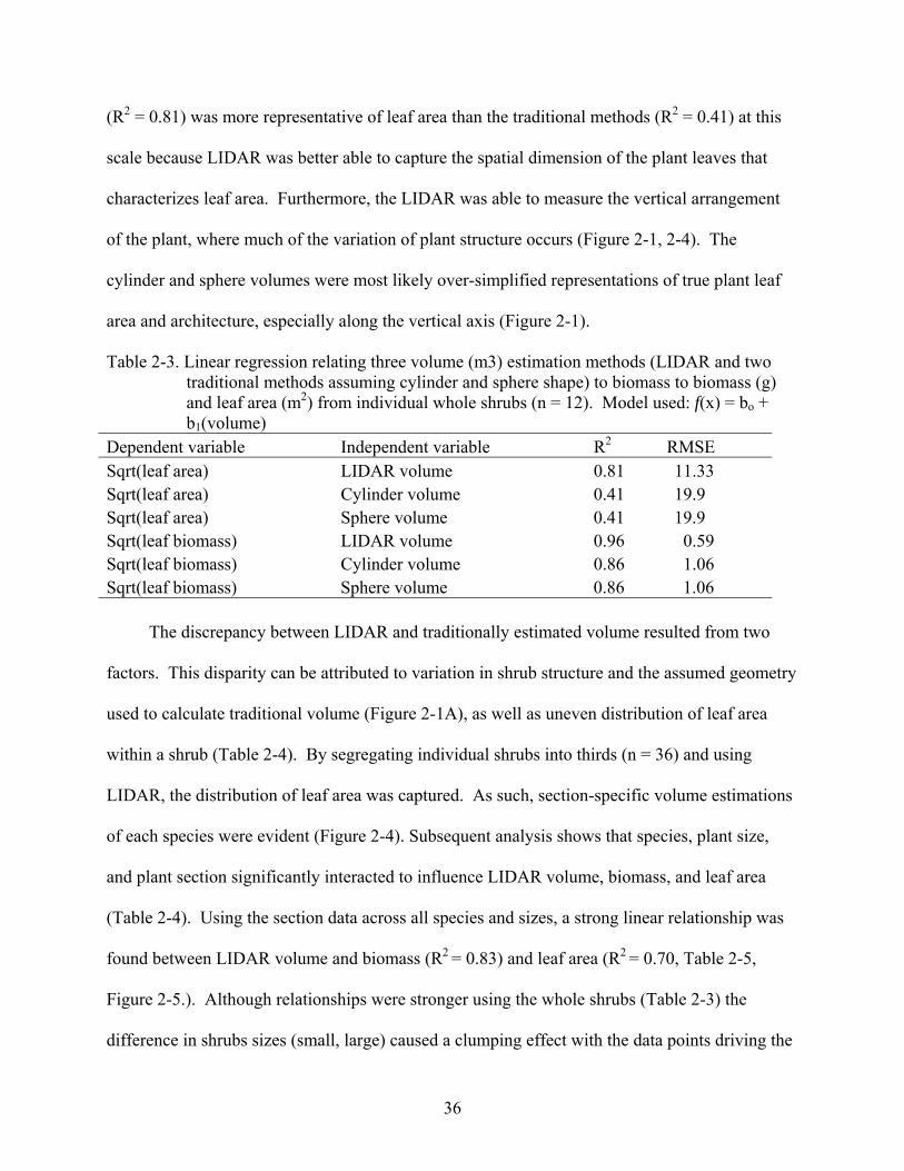
Table 2-3. Linear regression relating three volume (m3) estimation methods (LIDAR and two traditional methods assuming cylinder and sphere shape) to biomass to biomass (g) and leaf area (m2) from individual whole shrubs (n = 12). Model used: f(x) = bo + b1(volume)
Dependent variable Independent variable R2 RMSE Sqrt(leaf area) LIDAR volume 0.81 11.33 Sqrt(leaf area) Cylinder volume 0.41 19.9 Sqrt(leaf area) Sphere volume 0.41 19.9 Sqrt(leaf biomass) LIDAR volume 0.96 0.59 Sqrt(leaf biomass) Cylinder volume 0.86 1.06 Sqrt(leaf biomass) Sphere volume 0.86 1.06
The discrepancy between LIDAR and traditionally estimated volume resulted from two
factors. This disparity can be attributed to variation in shrub structure and the assumed geometry
used to calculate traditional volume (Figure 2-1A), as well as uneven distribution of leaf area
within a shrub (Table 2-4). By segregating individual shrubs into thirds (n = 36) and using
LIDAR, the distribution of leaf area was captured. As such, section-specific volume estimations
of each species were evident (Figure 2-4). Subsequent analysis shows that species, plant size,
and plant section significantly interacted to influence LIDAR volume, biomass, and leaf area
(Table 2-4). Using the section data across all species and sizes, a strong linear relationship was
found between LIDAR volume and biomass (R2 = 0.83) and leaf area (R2 = 0.70, Table 2-5,
Figure 2-5.). Although relationships were stronger using the whole shrubs (Table 2-3) the
difference in shrubs sizes (small, large) caused a clumping effect with the data points driving the

37
A
B
Figure 2-3. Linear relationships of leaf area measurements of all twelve individual whole shrubs with A) LIDAR volume and B) traditional volume estimates assuming a cylinder shape.
strength of the regression results (Figure 2-3). This suggests that knowledge of the vertical
arrangement of the plant as well as size is critical for accurately estimating plant volumes. The
accuracy of the LIDAR volume calculations (using a 3D moving window, see ‘Data Processing
and Analysis’) can be supported by the fact that the laser point-density distributions are directly
impacted by plant structure and size (Figure 2-1) when shadowing effects are minimized (i.e.,
using multiple scan angles). Shrub 3D spatial variability (related to volume, biomass, and leaf
R² = 0.81
0
20
40
60
80
100
120
0 0.005 0.01 0.015 0.02 0.025 0.03
Sqrt(le
af area (cm
2 ))
LIDAR volume (m3)
R² = 0.41
0
20
40
60
80
100
120
0 0.2 0.4 0.6
Sqrt(le
af area(cm
2 ))
Cylinder Volume (m3)

38
area) typically increases with size. This stresses the need for more accurate volume estimates of
complex understory fuelbeds, where shrub or other plant sizes vary and where volumes of larger
shrubs (> 0.5 m in height) may be more severely overestimated than smaller shrubs when using
traditional methods. These results could be critical for the successful application of ground-
based LIDAR for surface fuels assessments and represent a unique capability of LIDAR vis-à-vis
traditional methods. For example, applying this ground-based LIDAR approach for estimating
volumes at a larger plot or management unit level is foreseeable with the versatility of the MTLS
(e.g., truck and instrument mobility, vertical and horizontal angular positioning, ranging up to
1,500 m), especially within the open mid-story of this savanna-type woodland.
Overall, the use of this small cubic space (1 cm3) to calculate volume for the individual
shrubs proved advantageous for several reasons. First, the voxel approach minimized the
possibility of overestimating volume because the overlapping laser points that may have been
collected from the same plant canopy element (i.e., from merging of scans) were represented as a
single volumetric unit (cm3) rather than a raw point count. Hosoi and Osama (2006) concluded
that the ability to capture all of the plant canopy elements fully and evenly through the use of
several scans and scanning angles outweighs the possibility of overestimating volume, and such
overestimation is minimized by using a small voxel. Without multiple scans, volume may be
severely underestimated because of the significant loss of laser data on the ‘shadowed’ side of
the plant, which may require further statistical procedures to correct (Van der Zande et al. 2006).
This technique also provided the ability to measure volume at various scales of plant size as well
as estimate volume, leaf area, and biomass for various portions of the plant. This is especially
useful when plants are larger or highly complex in structure or shape and assumptions about
plant geometry (i.e., cylinder, spheroid) become less reliable.

39
Table 2-4. ANOVA output analyzing sectional shrub 1) LIDAR volume (m3), 2) biomass (sqrt-g), and 3) leaf area (sqrt-m2) estimates with three treatments: A) plant species (wax myrtle, saw palmetto), B) plant section (bottom, middle, top), and C) plant size (large, small)
1) LIDAR volume
Source term DF Sum of squares Mean square F-ratio Prob level
Power (α = 0.05)
A: species 1 4.70E-07 4.70E-07 0.28 0.603 0.080 B: section 2 8.83E-05 4.42E-05 26.12 <0.001* 1.000 AB 2 1.81E-05 9.07E-06 5.36 0.012* 0.791 C: size 1 4.68E-04 4.68E-04 276.55 <0.001* 1.000 AC 1 2.58E-07 2.58E-07 0.15 0.699 0.066 BC 2 5.45E-05 2.72E-05 16.11 <0.001* 0.999 ABC 2 1.60E-05 8.01E-06 4.74 0.019* 0.737 S 24 4.06E-05 1.69E-06 Total (adjusted) 35 6.86E-04 Total 36 2) Biomass
Source term DF Sum of squares Mean square F-ratio Prob level
Power (α = 0.05)
A: species 1 2.15 2.15 4.51 0.044* 0.532 B: section 2 50.53 25.27 53.10 <0.001* 1.000 AB 2 4.11 2.06 4.32 0.025* 0.695 C: size 1 67.34 67.34 141.51 <0.001* 1.000 AC 1 0.39 0.39 0.82 0.375 0.140 BC 2 8.64 4.32 9.08 0.001* 0.956 ABC 2 2.35 1.17 2.47 0.106 0.447 S 24 11.42 0.48 Total (adjusted) 35 146.93 Total 36 3) Leaf area
Source term DF Sum of squares Mean square F-ratio Prob level
Power (α = 0.05)
A: species 1 1199.63 1199.63 40.28 <0.001* 1.000 B: section 2 4544.19 2272.09 76.29 <0.001* 1.000 AB 2 191.04 95.52 3.21 0.058 0.557 C: size 1 4840.19 4840.19 162.52 <0.001* 1.000 AC 1 21.10 21.10 0.71 0.408 0.128 BC 2 757.72 378.86 12.72 <0.001* 0.992 ABC 2 272.65 136.32 4.58 0.021* 0.721 S 24 714.78 29.78 Total (adjusted) 35 12541.30 Total 36 * Term significant at α = 0.05

40
Figure 2-4. Mean volume and standard errors of vertical sections (equal thirds) of two pine-flatwoods shrub species (number of samples = 36; 12 plants, 3 sections each).
Table 2-5. Linear regression relating LIDAR volume (m3) to biomass (g), and leaf area (m2) from sectional shrub data. Model used: f(x) = bo + b1(LIDAR Volume).
Dependent variable n R2 RMSE Sqrt(leaf biomass) 36 0.83 0.87 Sqrt(leaf biomass), large shrubs only 18 0.78 0.96 Sqrt(leaf biomass), small shrubs only 18 0.60 0.56 Sqrt(leaf area) 36 0.70 10.51 Sqrt(leaf area), large shrubs only 18 0.62 12.02 Sqrt(leaf area), small shrubs only 18 0.33 8.03 n = number of samples
At the fuelbed scale (4 m x 4 m plots), the volume estimates from traditional point
intercept sampling and LIDAR were linearly correlated (R2 = 0.48; Figure 2-6) and were not
significantly different from one another (p = 0.12). The slope of the regression line was not
significantly different from a 1:1 relationship [CI (confidence interval) for slope ranged from
0.39 to 1.01; CI for intercept ranged from -0.5 to 2.87]. This suggests that fuelbed volume may
be estimated at sub-meter scales using either method with similar results. The lack of variation
0.000
0.002
0.004
0.006
0.008
0.010
0.012
Top Middle Bottom
Plant Section
Volu
me
(m3 )
Saw Palmetto
Wax Myrtle

41
captured in the model may be explained by the difference in sampling intensity (0.33 m vs.
~0.005 m) between the PI data and LIDAR data, respectively.
The aggregation of fuels within a fuelbed (and thus variance) influences the relative
accuracy of traditional point intercept sampling when compared to LIDAR. The empirical
variograms of the 4 m x 4 m plots illustrated that the spatial distribution of fuelbed heights
within a relatively small area (16 m2) was highly variable at multiple scales. This was illustrated
by the changing slope within the variogram plot (Figure 2-7). High spatial variation at very
small scales was observed (< 1 m lag distance). These small scale patterns in variation can be
observed within the variograms and were more evident within the LIDAR data compared to the
PI data (Figure 2-7A, D). Some plots displayed a distribution of spatial variance (e.g., Figure 2-
7B) indicating abrupt changes in fuelbed heights or with a hole in the variogram. These plots
consisted of a very low continuous fuelbed of grasses and forbs, with a few large inter-dispersed
shrubs (Figure 2-7E). The hole in the semivariogram represented the discontinuity of heights
between these different fuel types. Other plots had a more linear distribution of spatial variance
(Figure 2-7C), suggesting more consistently independent heights within the dataset. These fuels
were more randomly distributed with clustering only found within fuels found near the ground,
namely forbs, some grasses and pine litter (Figure 2-7F). The LIDAR data was determined more
reliable than the PI data for measuring surface fuel height distributions for two reasons. First, the
LIDAR data create a much lower nugget effect (errors of spatial variation or measurement) than
the PI data. Second, the LIDAR data were more sensitive to subtle changes in spatial heights at
fine-scales. This was seen by comparing the (non-spatial) variance (σ2) and spatial variance
(variogram) of fuelbed heights within a plot. The higher the σ2 the more likely the PI data
detected spatial changes in height, while the LIDAR data continued to detect changes at smaller

42
σ2 values [e.g., compare Figure 2-7B (larger variance) to Fig. 2-7 A,C (smaller variance)]. Not
surprisingly, this discrepancy is mainly because of the high concentration of LIDAR points
compared to those that can be obtained through PI methods. It is important to note that the field
effort to obtain this degree of accuracy through LIDAR was considerably less than that of point
intercept for all plots in this study.
A
B
Figure 2-5. Linear relationships of LIDAR volume estimates with A) leaf biomass and B) leaf area measurements of all twelve individual shrubs, divided into three equal vertical sections (n = 36).
0
10
20
30
40
50
60
70
80
0 0.004 0.008 0.012 0.016
LIDAR Volume (m3)
Sqrt(
Leaf
Are
a (c
m2 ))
R2 = 0.70
0
1
2
3
4
5
6
7
8
9
0 0.004 0.008 0.012 0.016
LIDAR Volume (m3)
Sqrt(
Leaf
Bio
mas
s (g
)) R2 = 0.83

43
Figure 2-6. Linear correlation between modeled volumes calculated from ground LIDAR and point-intercept (PI) field sampling. Solid Line: calculated regression line. Dotted line: 1:1 line.
Application
Ground-based LIDAR efficiently captured fine scale fuelbed characteristics related to plant
structure, specifically height and volume. Its precision compared to traditional methods is
explained by LIDAR’s ability to capture the actual vegetation structure versus an assumed
geometry. For discrete shrubs, ground-based LIDAR can accurately measure volumes which can
be used to derive biomass and leaf area. This is particularly useful in shrubby fuelbeds, such as
pocosin, chaparral or southeastern pine flatwoods, where destructive harvesting of fuels for
biomass is logistically difficult. In similar ecosystem types where prescribed burning is less
frequent (hence larger fuel buildup) or in larger plots or management units, this laser-technology
may still be applicable for estimating fuelbed volume. The surface grid technique of estimating
volume beneath a 3D rendering (used for the 4m x 4m plots) would be especially useful. The
size of the area that can be captured with the MTLS is only bound by time for data collection and
processing and hard drive space. Shadowing effects however, seem to be the limiting factor
LIDAR Volume (m3)
0 2 4 6 8 10
PI V
olum
e (m
3 )
0
2
4
6
8
10
R2 = 0.48

44
when capturing distinct spatial plant structure and may become more difficult to obtain where
fuels are thicker or denser. This can be minimized with multiple scans (particularly from
elevated positions), careful positioning of the MTLS, and thorough processing techniques
(merging of scans and removing trees).
Costs were quite minimal ($350 per day for data collection with the MTLS) considering
the nominal data acquisition time for a large amount of information. For reference, all the shrub
data was collected in less than one day, while all 26 4 m x 4 m fuelbed plots were collected in
two days. Each fuelbed plot took approximately 15 to 30 minutes each plus travel time to each
plot. For comparison, point-intercept data collection took 2 to 3 weeks. Although data
processing was quite involved (with various software packages and engineering expertise
required) for the LIDAR data, the procedure was similar to aerial LIDAR processing and was
included in the cost. The time needed for data entry from (4 m x 4 m plot) field recordings and
LIDAR data processing was approximately the same (~ one hour per plot). Ultimately, the
LIDAR data required more expertise in understanding, recording, and processing of the data than
the point-intercept approach, but the outputs were an order of magnitude more precise, which
may provide for detailed information to relate to fine-scale fire behavior.
Fire behavior prediction system software is sensitive to fluctuations in parameters
associated with fuelbed height measurements, such as calculating volume and fuel density
(Andrews and Queen 2001, Scott and Burgan 2005). Volume is especially difficult to measure,
compared to mass estimates in many fuelbeds, because of the complex structure. As shown in
this study, LIDAR provides an opportunity for improving measurements of fuelbed properties
that drive fire behavior and possibly enhance the accuracy of fire behavior prediction models.
Moreover, LIDAR has the capacity to measure those characteristics with a precision and at a

45
finer scale than is afforded by traditional methods. The degree to which such fine scale
heterogeneity is critical to fire behavior and fire effects is not currently known but can only be
tested by the development of methods with the capacity for such measures. This approach to
using ground-based LIDAR is promising in this aspect, as both measurements of the physical
structure of fuelbeds and discrete fuel types can be sampled non-destructively and analyzed in a
spatially explicit context. By understanding how fuel structure and fine-scale volume vary
among fuels, other fuel characteristics, such as surface area to volume ratios, packing ratio, fuel
continuity, and patchiness can be examined in detail for effects on fire behavior.

46
Figure 2-7. Examples of spatial variation (empirical variogram) of fuelbed heights found within three 4 m x 4 m plots recorded by point intercept (PI) field sampling and ground LIDAR. Here it is illustrated: A) how spatial variation may only be evident using the LIDAR data, B) how strong correlations between LIDAR and field sampling may be found where spatial variation is large compared to other plots (0.45 vs. 0.12 m2 for B vs. A, respectively) and strong fluctuations of spatial continuity (i.e., low fuels with inter-dispersed shrubs) across the plot, and C) how an overall low (< 0.06 m2) height variation (compared to A,B) may only be evident using the LIDAR data, where fuels may be continuous past a range of 1 m. LIDAR imagery (D-F) provide a 3D visual representation of fuelbed height distributions and height (m) statistics associated with each variogram (A-B), respectively. Note scale is different between graphs and color gradients in the LIDAR imagery are relative to vertical height distributions within each plot.
0.00
0.04
0.08
0.12
0.16
0.0 0.5 1.0 1.5 2.0 2.5 3.0
Var
iogr
am (m
2 )
Lag Distance (m)
0.00
0.10
0.20
0.30
0.40
0.50
0.0 0.5 1.0 1.5 2.0 2.5 3.0
Var
iogr
am (m
2 )
Lag Distance (m)
PI dataLIDAR data
Max ht = 2.5 m σ2 = 0.26 E
Max ht = 1.8 m σ2 = 0.11
D
A
B

47
Figure 2-7. Continued.
0.00
0.02
0.04
0.06
0.08
0.0 0.5 1.0 1.5 2.0 2.5 3.0
Var
iogr
am (m
2 )
Lag Distance (m)
PI dataLIDAR data
Max ht = 1.5 m σ2 = 0.09 F
C

48
CHAPTER 3 RELATING FINE-SCALE FOREST FUELBED STRUCTURE AND TYPE TO FIRE
BEHAVIOR USING GROUND-LIDAR, THERMAL IMAGING, AND REGRESSION-TREE MODELING
Introduction
Fuel and Fire in the Longleaf Pine Ecosystem
Longleaf pine savannas of the southeastern U.S. are linked to frequent low-intensity fires
(Agee 1998). Longleaf pine and many of the understory grass and forb species depend on fire to
reduce competition from faster growing shade-tolerant plants and create an ideal soil
environment for successful regeneration (Myers 1990). The grassy understory is relatively low
in stature (0.5 – 1.5 m) creating a bed of fine fuels that carry a low-intensity fire through the
forest. Although this fuelbed – defined here as the understory vegetation or surface fuels that
carry fire (DeBano et al. 1998) – seems homogeneous at first glance, fuel types and structure are
diverse at fine scales (i.e., within a few meters). The dynamics between this heterogeneous fuel
environment and the regulation of future vegetation by fire has been referred to as the ecology of
fuels (Mitchell et al. 2009). This concept emphasizes the importance of fuels as a link between
the combustion environment and vegetation response. More specifically, it targets a need for
understanding the ecological significance of fine-fuels (especially pine-litter) and quantifying
fuels and fire behavior at the appropriate scale (Hiers et al. 2007, Mitchell et al. 2009). The
appropriate scale is ultimately determined by the spatial range of their inherent heterogeneity or
variation (Hiers et al. 2009, Loudermilk et al. 2009). The variation within the fuelbed is
characterized by vegetation fuel types, structure, biomass, and condition (e.g., moisture content).
Fuel types in this study included wiregrass (e.g., Aristida stricta, A. beyrichiana,
Sporobolus junceus), other grasses, forbs, ferns, woody shrubs (Quercus falcata, Q. incana, Q.
laevis, Persimmon spp., Rubus spp.), pine litter, shrub litter, and various downed woody fuels.

49
One fuel (or non-fuel) type in particular is characterized by patches of bare-soil, most often
represented by turned up soil mounds from ground-dwelling pocket gophers (Geomys pinetis)
and less frequently by gopher tortoises (Gopherus polyphemus). Pocket gophers can be
abundant, creating a bare soil mound every few meters and found scattered across a longleaf pine
stand (Simkin and Michener 2005). This unique fuelbed characteristic may act as a small fire
break inadvertently influencing plot-level fire behavior (Hiers et al. 2009).
Fuelbed fires are also influenced by vegetation structure, which is a product of plant size,
height, shape, leaf area, or spatial distribution. These structural attributes represent fuel volume
and biomass, hence the amount of energy available to burn. Their spatial size and leaf area
distribution directly influences their energy loss rate as a fire passes through (Ryan 2002).
Wiregrass distribution is especially pertinent in this structure. The understory is often noted as
having a ‘sea’ of wiregrass, where its bunchy plant form creates a wave-like, but continuous
fuelbed not often exceeding 1.5 m in height. Taller woody shrubs are often peppered throughout
this grassy understory, further altering fuelbed structural properties. Pine-needle litter cast from
the overstory becomes intertwined with the spike-like wiregrass blades to form a mesh fuelbed.
This creates an oxygen rich environment with easily ignitable and continuous fine fuels,
important for fire spread (Myers 1990).
Fuelbed depth (or vegetation height) is an important structural component that represents
abundance and continuity of fuels. Depth may range from only a few centimeters to about two
meters in a frequent fire regime. Fuel types vary along this height gradient. Leaf litter may
cover the first few cm of the sandy soil bed, while grasses, small shrubs, and forbs may be found
as intermediate sized fuels. Taller shrubs and longleaf seedlings may break up the fuelbed further
altering fuelbed structural characteristics. Perched leaf litter – litter draped on top of and

50
hanging within the plant fuelbed – is also found along this height gradient. Shrubs taller than
about two meters have most likely escaped the lethal fire flames (Rebertus et al. 1989), where
they are no longer a part of the surface fuels, hence unavailable as combustible energy. As such,
estimating fuelbed structure components is complex, but essential for relating to fire behavior at
the same scale.
Measuring Fuelbed Structure
Vegetation structure is one of the more difficult aspects of the surface fuelbed to measure
due to the complexity in plant architecture. Surface fuelbed characteristics have traditionally
been quantified by both direct and indirect methods. Direct measurements commonly employed
are tallies of down woody fuels along planar transects (Brown 1974), and coupled destructive
biomass sampling (i.e., “clip plots”) (Brown 1981). Indirect methods include visual cover
estimates in plots or comparisons with photographs of known fuel loads or types (Ottmar et al.
2003, Keane and Dickinson 2007). These methods allow for stand level estimation of variables,
such as fuel load, bulk density, and packing ratios that are then used to predict fire behavior
(Reinhardt and Keane 1998, Andrews et al. 2004).
Each method has significant limitations. Direct sampling is labor intensive often limiting
sample size. Some techniques are not appropriate for all fuel types: Planar transects are not
efficient at estimating fine fuels such as grasses. Indirect measures can be subjective, resulting
in biased estimates. A plant’s architecture is often simplified into general geometric shapes such
as a spheroid or cylinder (Van Wagner 1968) to estimate volume for bulk density calculations.
While these approaches are recognized to have inherent limitations, no alternatives were
previously available.
Recent advances in laser ranging, or LIDAR, technologies have enabled the successful
measurement of complex structures in the field with both high accuracy and precision

51
(Hopkinson et al. 2004). LIDAR has been typically used in forestry for coarse scale remote
sensing of forest canopy structures, estimating tree height distributions, canopy bulk density, and
leaf area (Lefsky et al. 1999, Drake and Weishampel 2000, Hall et al. 2005, Roberts et al. 2005,
Lee et al. 2009). These airborne LIDAR approaches have been unsuited, however, in measuring
understory vegetation, primarily because of the obstruction from the forest canopy and a
horizontal resolution limited to the few decimeter scale. Modern ground-based LIDAR systems
now have many of the strengths of airborne systems (in particular laser pulse rates of a few
thousand Hz or more that enable high-resolution sampling), but they can attain sub-centimeter
resolution and be positioned under the canopy to reduce the shadowing effects of overstory trees
(Slatton et al. 2004). The high-density three-dimensional (3D) point data (more than 10,000
points per m2) obtained from such systems provide the needed precision to characterize fuelbeds,
particularly by quantifying fuel height distributions, fuel density and volume measurements.
These data also provide the means to develop a multitude of LIDAR based fuel metrics based on
the vertical and horizontal distribution of vegetation.
One system in particular, the Mobile Terrestrial Laser Scanner (MTLS), is a static, stop-
and-scan laser scanner that covers a limited area, but captures data at the sub-cm level. The
MTLS consists of Optech’s ILRIS 36D (Intelligent Laser Ranging and Imaging System) ground
based laser scanner (Lichti et al. 2002, Fröhlich and Mettenleiter 2004), which was mounted on a
lift atop a mobile platform (4 x 4 truck) by the National Center for Airborne Laser Mapping
(NCALM) at the University of Florida. The MTLS captures details about the terrain at multiple
angles. The ability to vary the LIDAR height and pointing angle using the MTLS allows
significant reduction in shadowing effects that may be found when using a LIDAR system on a
tripod.

52
Ground-based LIDAR (also called terrestrial LIDAR) has only recently been used in
forestry applications. Accurate tree and canopy metrics (e.g., timber volume, tree height and
diameter, gap fraction) have been successfully estimated using tripod mounted terrestrial LIDAR
systems (Hopkinson et al. 2004, Watt and Donoghue 2005, Henning and Radtke 2006). Fine-
scale leaf area (Lovell et al. 2003, Tanaka et al. 2004) and gap fraction (Danson et al. 2007)
estimates of tree canopies have been correlated to that of hemispherical photographs. Small
individual trees were measured using a voxel-based approach to determine leaf area density at
the mm3 scale (Hosoi and Omasa 2006). Ground-based LIDAR has also been used to understand
the impacts of instrument positioning on shadowing effects that influence tree canopy
measurements (Van der Zande et al. 2006). Although most terrestrial LIDAR systems used in
forestry are stationary, a portable LIDAR system has been developed to record 1 m scale canopy
measurements while moving through a forest (Parker et al. 2004). Only recently has ground-
LIDAR been used to characterize the surface fuelbed, demonstrating the importance of
measuring and accounting for plant structure in volume estimates as well as understanding the
spatial variability of fuelbed heights at small scales (Loudermilk et al. 2009).
Relating Fuelbed to Fire Behavior
Fuelbed structural components, e.g., plant heights, height variation, volume, volume
distribution, are important drivers of fire behavior from the plant to landscape level (DeBano et
al. 1998, Mutlu et al. 2008). Assessing relationships between fuels, fire, and fire effects are,
however, generalized to the stand or landscape level often assuming homogeneity at any finer
scale. This assumption ignores the spatial heterogeneity of fuels and fire behavior within the
fuelbed that influences overall plant community dynamics (Hiers et al. 2009). Quantifying the
fire environment has been focused on visual estimates of flame length (Hoffmann and Solbrig
2003, Kennard et al. 2005, Robertson and Ostertag 2007) which is subjective, may be obscured

53
by smoke (Fernandes et al. 2000), and unrepresentative of the heating environment needed for
fuel combustion (Hiers et al. 2009). Thermocouples or temperature-sensitive paints have been
used for point-source measures of fire intensity allowing for interpolation to larger scales.
Although these measures have been useful, estimates of fire intensity have been compromised
because of issues with instrument measurement lags causing erroneous low combustion
threshold temperatures (Iverson et al. 2004, Kennard et al. 2005). Furthermore, the recordings
are spatially limited and therefore intricate measurements of heterogeneity are lost.
Thermal videography (i.e., FLIR – Forward Looking Infrared imaging system) is a
promising technique, which overcomes some of the aforementioned shortcomings by recording
precise temperatures in a spatially and temporally explicit context. Its thermal signature range is
similar to remote sensing sensors that collect data beyond the visible light spectrum, yet specific
for fire temperature readings (wavelengths 7.5 to 13 μm). FLIR has been used for many years by
the United States Department of Agriculture Forest Service for airborne fire detection and fire
mapping over large areas, benefitting from its thermal sensitivity and smoke penetration
capabilities (Krausmann and Hicks 1996). Here, the FLIR has been used to analyze fire line
conditions and determine safe and efficient strategies to combat wildfires. It has also been used
to measure fire plumes of chaparral shrubs in a laboratory setting (Sun and Weise 2003). Just
recently has the system been used to measure surface fires at the plot level (Hiers et al. 2009).
Ground-based LIDAR and FLIR technologies have the means to capture the variability of
fuelbed structure (continuity) and fire behavior at very high-resolutions (Figure 3-1).
Interestingly, fuel and fire heterogeneity varies along the same distance gradient (~ 1 to 1.5 m)
(Mitchell et al. 2006). After about 1 m, the fuels and fire behavior become relatively
homogeneous, illustrating little to no properties of spatial autocorrelation (Hiers et al. 2009,

54
Loudermilk et al. 2009). The relationship between the fuelbed structure and specific fuel types
to fire behavior properties at this fine scale has been unknown and unachievable thus far due to
the bottleneck of limited measurement capabilities and difficulty in assessing their multifaceted
relationships.
Figure 3-1. Fine-scale spatial heterogeneity of A) fuelbed structure (depth, m) and B) fire behavior (temperature in °C) recorded within the longleaf pine-wiregrass system used in this study. These modeled (exponential) semivariograms were created from in situ data on fuelbed depth and fire temperature in 4 m x 4 m plots captured from LIDAR (Light Detection and Ranging) and FLIR (Forward Looking Infrared) remote sensing instruments, respectively.
Regression-Tree Modeling
The relationships between fuel structure (fuelbed depth, leaf and stem distribution, surface
to volume ratio, continuity) and the fire environment (combustion properties, weather) are
complex and non-linear. In a longleaf pine savanna, fires are of relatively low intensity with
typical flame heights below a few meters (Robertson and Ostertag 2007). Slightly taller shrubs
(> 2 to 3 m) may escape a passing fire and fuel combustion may only occur beneath or nearby
the shrub canopy, consuming surface fuels, such as bunch grasses, smaller shrubs, and leaf litter.
Burn characteristics within this area may not correlate highly with typical fuel measurements
(e.g., biomass) because of the patchiness of the burn. These intricate relationships are difficult to
0.0
0.1
0.2
0.0 0.5 1.0 1.5 2.0
Sem
ivar
ianc
e of
fuel
bed
dept
h
Distance (m)
0
1000
2000
3000
4000
5000
6000
7000
0.0 0.5 1.0 1.5 2.0
Sem
ivar
ianc
e of
fire
tem
pera
ture
Distance (m)
A B

55
quantify and traditional multivariate regression approaches used to explain their interactions or
develop predictive models may not be appropriate for such multifaceted relationships (Grunwald
et al. 2009).
Regression tree modeling (also known as ‘tree-based modeling’) provides an alternative
approach to multivariate regression, designed specifically for complex non-linear relationships.
Satisfying typical regression assumptions related to input variables, residuals, and sample
distributions is essentially unnecessary in tree-based models, due to their ability to partition the
predicted variation of the independent variables into autonomous predictors (Breiman et al.
1984). The CART (Classification and Regression Tree) software (v. 5.0, Salford Systems, San
Diego, CA) follows this partitioning of variation in a binary recursive approach, where parent
nodes (representing all or a portion of the unexplained variation) are always split into two child
nodes. These two nodes represent the splitting of the variation – typically into lower and higher
portions – based on the associated predictor value. These child nodes are recursive as they can
become parent nodes and repeat the process to eventually create relatively homogenous (low
deviation) terminal nodes. The means of the values within each terminal node are the model’s
predictors (Grunwald et al. 2009). CART can be used to either categorized features (similar to
land cover classes in remote sensing) or to predict continuous variables (similar to regression)
using categorical or continuous input variables for both.
Tree-based modeling has been extensively used in environmental studies to unravel
relationships between large numbers of independent variables that may all contribute in part to a
particular environmental or landscape phenomenon. They have been especially important for
predicting soil attributes, such as organic carbon (Vasques et al. 2009) and phosphorus loading
(Grunwald et al. 2009) as well as assessing hydrological trends, such as rainfall-runoff modeling

56
(Solomatine and Dulal 2003) and understanding water level-discharge relationships
(Bhattacharya and Solomatine 2005). Tree-based modeling is a promising tool in ecological
studies, used successfully for classification applications of forest land cover predictions (Moisen
and Frescino 2002), vegetation mapping under various climate scenarios (Prasad et al. 2006), as
well as determining abundance distributions of soft coral taxa (De'ath and Fabricius 2000). To
date, regression trees have not been used for assessing forest fuel and fire behavior relationships.
The objective of this study was to examine the fine-scale relationships of fuelbed structure
(from ground-LIDAR) and fuel types (from in situ data) to fire behavior characteristics (from
FLIR) across multiple forest fuelbed plots within a longleaf pine-wiregrass ecosystem. More
specifically, the predictive power of various ground-LIDAR fuel metrics coupled with fuel type
data were analyzed for determining surface fire temperature and residence time at sub-meter
scales using regression-tree modeling. Relationships were examined at various grouped-plot
levels and within representative individual plots. Another objective was to assess potential
technical and modeling pitfalls as well as determine the implications for assessing fine-scale fire
effects.
Methods
Ground-LIDAR (Light Detection and Ranging) Instrumentation
The ILRIS ground-based LIDAR system uses a 1535 nm wavelength (near-infrared) laser
with a frequency of 2,000 Hz (pulses per second), recording first or last returns of each laser
pulse (user defined). The maximum field of view is 40˚ in both horizontal and vertical plane,
although smaller fields of view can be specified for a given scan. The system can register laser
returns from 5 to 1500 m away (at 80% target reflectivity). The ILRIS used in this work has a
pan-tilt base on the MTLS, which allows for a 360˚ rotation in the horizontal plane and roughly
±40˚ in the vertical plane. The lift on the MTLS provides for a vertical adjustment of the scanner

57
up to a height of about 9 m. Recording laser data from multiple positions around the target will
reduce information lost from shadowing effects, but an efficient imaging geometry is desired to
minimize the number of scans required to sample each plot. The ability to adjust the instrument
vertically and horizontally to the extent offered by the MTLS allows the user to achieve
advantageous scan positions and orientations in spite of constraints posed by the terrain or
nearby occluding trees, which is essential to measuring precise fine-scale attributes of intricate
plant structures (Hosoi and Omasa 2006).
Point density in LIDAR point clouds will vary locally depending on the range from the
laser to objects in the field of view and on the angular spacing of laser shots. For the ILRIS
sensor, the pulse rate is fixed at 2000 Hz. The angular separation of laser pulses is used to
achieve a desired point density, which is input via the ILRIS Controller software. To achieve
this, the ILRIS pre-scans the user specified field of view at a course resolution and acquires an
average range. The user then enters the desired linear point spacing into the ILRIS Controller
software. This spacing corresponds to the average linear separation between points on a
hypothetical plane segment that spans the user specified field of view, is located at the mean
range, and is orthogonal to the sensor’s boresight. Given this separation distance and the mean
range, the necessary angular shot spacing is automatically calculated by the ILRIS Controller
software. Under typical operating conditions, the linear point spacing is chosen to be anywhere
from a few cm to 1 mm. High point densities come at the cost of increased memory to hold the
data and increased time to complete the scan. For example, a 20˚ × 20˚ field of view centered at
boresight with a mean range of 15 m and user specified linear point spacing of 5 mm will yield
an angular separation of 0.0189˚, require roughly 9 min to complete, and result in just over 1.1
million points.

58
The ILRIS collects: 1) x, y, z coordinate values with respect to the position of the laser
sensor; 2) intensity values of the return; and 3) true color (Red Green Blue) values for each point
obtained from an integrated and calibrated digital camera within the instrument. A more
complete description of the technology can be found in (Lichti et al. 2002, Fröhlich and
Mettenleiter 2004). Once an area is sampled by two or more scans, the point clouds from each
scan are merged into a common coordinate frame using software that can accommodate 3D
spatial data. The subset of the point cloud that covers the region of interest can be isolated and
the remaining points cropped out to minimize the computational burden and obtain statistics
representative of the precise region of interest.
Study Site
The site was located at Ichauway, an 11,000 ha reserve of the Joseph W. Jones Ecological
Research Center in southwestern Georgia, USA. Ichauway is classified within the Plains and
Wiregrass Plains subsections of the Lower Coastal Plain and Flatwoods section (McNab and
Avers 1994). Ichauway has an extensive tract of second-growth longleaf pine and has been
managed with low intensity, dormant-season prescribed fires for at least 70 years, at a frequency
of one to three years. The understory of the study area was primarily composed of wiregrass
(Aristida stricta), many forb and prairie grass species, as well as inter-dispersed hardwood
shrubs (e.g., Diospyros spp., Prunus spp, Quercus spp., Sassafras albidum). With frequent fires,
hardwoods are generally maintained at shrub size, occasionally reaching mature size. The study
area had not burned for one year.
Data Collection
In spring 2007, a total of 20 georeferenced 4 m x 4 m plots were established to measure
fuelbed characteristics. The 4 m x 4 m area was chosen because it was large enough to capture
heterogeneity at sub-meter scales, but small enough to support intensive sampling with minimal

59
impact to the vegetation. A ladder was suspended horizontally across the plot to sample the
interior with minimal disturbance to the vegetation. Spatially explicit point-intercept (PI) fuel
data (169 samples, 0.33 m grid spacing) were recorded using a 5 mm graduated dowel within
each plot. Only vegetation in physical contact with the dowel was measured. At each PI sample
point, maximum fuelbed and litter depth (or height), as well as presence/absence of fuel and
vegetation types were recorded. The georeferencing and sampling intensity were used to capture
the spatial variation of the fuelbed found within this small (16 m2) area and to relate to the sub-
centimeter scale 3D laser data collected from the ground-based LIDAR.
Within two weeks of field data collection, the MTLS was used to collect ground-LIDAR
data on all 20 plots. Prior to laser data collection, reference targets (consisting of a styrofoam
ball on top of a metal rod, 0.5 to 1 m tall) were placed at all four corners of the plot. A double
reference target (two Styrofoam balls on one metal rod) was used at the northwest corner of each
plot to orient the plot data for processing. The MTLS was restricted to mapped roads and trails,
as well as a buffer of 5 meters around each plot, to reduce vegetation disturbance. The ILRIS
was lifted to a height of 7 m to capture an aerial view of the plot to reduce shadowing effects and
avoid tree bole or canopy obstruction. The ILRIS was set to a downward angle tilt of 25° from
horizontal. A true color digital photograph was taken by the ILRIS for each plot, and used in the
field to delineate the precise field of view for each scan. First-return laser pulses were recorded
with an input mean point spacing of 5 mm. Two scans were taken of each plot, from opposite
sides, to mitigate shadowing effects and ensure more accurate and complete sub-centimeter scale
data for fuel plots. These two scans were merged in the processing stage to a single 3D point
cloud data set. Data collection with the MTLS took approximately 20 minutes per plot. In
comparison, field PI data collection lasted an average of two hours per plot.

60
In each plot, fire behavior was recorded using a FLIR S60 digital thermal imagery system.
The camera and operator were positioned on a boom about 7 m above the ground and 10 m from
the plot edge. Thermal images were captured as the controlled fires burned through the plots at
0.25 Hz. A 0.5 x lens was attached to the camera to increase the field of view and record
temperatures for the entire plot simultaneously. The camera has two temperature range settings
(-40 to 500º C or 300 to 1500º C); the latter (higher) temperature range was used here. The
measurements were corrected for air temperature, relative humidity, distance from target, and the
emissivity was set at 0.96. A flare was placed at each plot corner and ignited immediately before
the fires to provide surveyed reference points for post data processing. Further details are in
Hiers et al. (2009).
All plots were burned during three prescribed burns conducted at an operational scale
(about 70 ha each) using strip head fires on February 23, 27 and March 16, 2007. A strip head
fire was ignited 5 m upwind of each plot with over 100 m separating strip heads from downwind
strips when plots were ignited. Plots within a burn unit were burned and sampled from
downwind to upwind. Each operational strip head fire was allowed to burn through the plots
undisrupted by additional lines of fire (Hiers et al. 2009). Mean wind speed and temperature
were quite similar between days, ranging from 1.47 to 2.19 m/s and 19.4 to 22.9 º C, respectively
(Table 3-1). Plot level wind speeds were recorded during the fire (Table A-1). The mean plot
level wind speed values ranged from 1.1 to 2.9 m/s. Relative humidity on the other hand was
quite different between days, ranging from 14.9 to 65.9 %.
Table 3-1. Burn day mean wind speed (m/s) and direction from wind sensors next to each plot as well as mean temperature and relative humidity (RH) from a local weather station.
Burn date Wind speed Wind direction Temp. (°C ) RH (%) No. plots February 23, 2007 1.80 South 19.36 14.88 5 February 27, 2007 1.47 Southwest 22.88 42.28 7 March 16, 2007 2.19 Southwest 22.06 65.86 8

61
Data Processing
The presence or absence data for each fuel type collected in the field (PI data) were
represented as categorical binary variables (1 = present, 0 = absent) for each spatially explicit
point (33 cm spacing) within each plot. These binary fuel type variables were used as (11)
independent variables in the statistical analyses (e.g., CART). The point-intercept data across all
plots were converted to distance matrices for use in cluster analysis (Hiers et al. 2009) .
Euclidean distances were used for continuous variables (fuelbed height, litter height), whereas
asymmetric Jaccard distances were used for the 0 or 1 binary variables (presence or absence of
longleaf pine litter, etc). The Jaccard distance measured the overlap of presence (similarity) of
various fuel types, while Euclidean distance measured the degree of continuity of fuelbed or
litter depths. Cluster trees were then calculated using the centroid method, and the number of
clusters was selected based on the Cubic Clustering Criterion and Pseudo-F value traces (Everitt
1980). In the case of multiple local maxima for these criteria, the cluster groups were compared
with known plot characteristics to select the final number of clusters (SAS Institute Inc. 2003).
This process is similar to development of fuelbeds at larger scales (Dimitrakopoulos 2002). The
(11) clusters [detailed in Hiers et al. (2009)] represented a variety of fuel types ranging from
patches of bare ground and coarse woody debris to complexes of pine litter, shrubs, and grasses.
The most common fuels clusters were mixed graminoids, wiregrass with shrubs, and wiregrass
with perched longleaf pine litter.
The ‘Quick Terrain Modeler’ (Applied Imagery) and ‘TerraScan’ (Terrasolid) software
packages were used for processing the laser data. Of the two scans taken per plot, the first was
horizontally rectified by compensating for the original scanning geometry, since the instrument
had a downward tilt of 25° with respect to horizontal. The reference targets were used to identify
common points between the two scans and create a common 3D coordinate frame for both scans

62
(see (Wolf and Ghilani 1997) for details). The second scan was adjusted to fit the same 3D
coordinate frame as the first, which combines them into a single spatially consistent data set. The
digital image and the double target reference for the northwest corner of the plot were especially
helpful in this merging process and in orienting the plot in cardinal space. The 4 m x 4 m plot
areas were clipped from the resulting merged scans using the reference targets. Roughly 600,000
to 700,000 sample laser points were found within each 4 m x 4 m plot (Figure 3-2).
A B
Figure 3-2. Example outputs of the A) ground-based LIDAR (using the MTLS) and the B) thermal camera (using the FLIR) for a 4 m x 4 m forest fuelbed plot. The color gradient in A represents the vegetation height distribution (maximum vegetation height = 4 m), which aids in visualization of the 3D vegetation structure. Blue and green represent lower vegetation, leaf litter and ground points, while yellow and red represent taller vegetation.
The ground-LIDAR data were scaled down to the spatial resolution (33 cm x 33 cm) of the
PI data. This is a commonly used approach for aerial LIDAR data, where LIDAR metrics were
calculated within equally spaced vertical sections or bins (e.g., pixels) (Goetz et al. 2007). Using
MATLAB (The MathWorks, Inc.) 13 LIDAR related metrics were determined based on the
distribution of ground-LIDAR laser points and intensity values found within each bin (Table 3-
2). LIDAR height (z) values calculated within each bin included mean, maximum, variance,
kurtosis, skewness, distribution ratio (mean/max), sum, and spread (max-min). The various

63
height distribution values (e.g., skewness, kurtosis) represented unique structural features of the
fuels not represented by the more common attributes (e.g., mean, max) and test their relationship
Table 3-2. Fuelbed [ground-LIDAR (Light Detection and Ranging) and point-intercept] and fire (FLIR – Forward Looking Infrared) metrics created for the CART (Classification and Regression Tree) analysis. Metrics were determined within 33 cm x 33 cm cells within 20 4 m x 4 m forest plots. All height values are in meters and point-intercept data are categorical. All intensity and point density values are normalized across all plots.
Fuelbed metrics Fire metricsGround-LIDAR Point-intercept FLIR x, y coordinatesa Fuel Clusters (1-11)b Maximum temperature °CMean height Fuel types (0/1): 90th quantile temperature °CMaximum height 1 and 10 hour fuels (HR 10) Residence time above 300°CVariance of height 100 and 1,000 hour fuels (HR 100) Residence time above 500°CKurtosis of height Pine litter Skewness of height Oak litter Height distribution ratio (mean/max) Perched pine litter Sum of heights Perched oak litter Spread of heights (max - min) Wiregrass Point density (0-1) Other grasses Mean LIDAR intensity (0-1) Forbs Intsqrt [sum of sqrt(LIDAR intensity)] Shrubs Intqdrt [sum of qdrt(LIDAR intensity)] Volatile shrubs Intlnr [sum of LIDAR intensity] Bare soil (no vegetation/fuel) a used for plot level analysis only; b used for multi-plot (collective and grouped) analysis only, HR = hour, sqrt = square root, qdrt = quadratic
with the fire metrics. Laser point density values and LIDAR intensity values were normalized
across all plots by dividing each bin’s value by the maximum value across all plots. Three
additional intensity variables were created to represent the interaction of volume of fuel (i.e.,
laser point density) and type (leaf surface area) or condition (moisture) of the fuel (i.e., LIDAR
intensity). LIDAR intensity values have been used to differentiate between broad and narrow
leaved trees species and been correlated with fuel moisture (García et al. 2010), but the
relationship with surface fine-fuels is unknown. One variable was simply the sum of the
normalized LIDAR intensity values (intlnr = inti/intmax, i = individual laser point) within each bin

64
(linear relationship between intensity value and point density), while the other two were
normalized (as above) and scaled by the quadratic (Equation 3-1) and square root (Equation 3-2)
function and summed individually within each bin (i.e., intqdrt, intsqrt , respectively). This scaling
represented a range of degrees that the backscattered pulse may be influenced by the volume or
density of fuels found within each 33 cm x 33 cm area. The quadratic function suppressed the
influence that the amount or size of fuel (point density) had on LIDAR intensity compared to the
linear relationship. The opposite was true for the square root function.
∑ (3-1)
∑ (3-2)
The FLIR fire images were analyzed using FLIR Systems’ ThermaCAM Researcher Pro
software version 2.7 (Figure 3-2). Each image was then transformed into a tab-delimited ASCII
file where each cell represented pixel temperature. These files were again transformed into TIFF
files for post-processing, with the temperature data in these files captured as pixel color values.
The TIFF files were rectified and georeferenced using image processing software (Geomatica).
Summary statistics over time (represented by the multiple image captures by the camera) were
computed for each pixel in the original thermal imagery data, including maximum temperature
(Tmax), 90th quantile temperature (Q90), residence time above 300°C (T300), and residence time
above 500°C (T500). The Q90 temperature data were used to analyze the thermal imagery
because the lowest temperature measured on the camera’s high-temperature setting was 300°C;
thereby, Q90 distinguished unburned patches from smoldering fire (Hiers et al. 2009). The two
residence time variables potentially segregated the smoldering effects of fire into low (T300) and
higher (T500) smoldering intensities. These resulting FLIR datasets of temperature and

65
residence time were also scaled down (from about 4 cm x 4 cm) to the 33 cm x 33 cm spatial
resolution of the PI (and now ground-LIDAR) dataset by averaging each of the four fire metrics
within each bin.
Grouping of Plots
All twenty plots were grouped based on their fire behavior metrics using a k-means cluster
analysis. Each plot was represented by their standardized mean value for each of the four fire
metrics. The number of clusters was chosen based on the Cubic Clustering Criterion and Pseudo
F statistic. There were clearly three distinct clusters among the plots, representing three levels of
fire intensity (Figure 3-3, Figure 3-4). The first group represented the middle range of
temperatures and residence times corresponding to nine of the twenty plots. The second cluster
represented the higher range of temperatures and residence times, while the third cluster
represented the lower range, corresponding to five and six plots (out of twenty), respectively.
This plot grouping provided for a streamlined data analysis approach to analyze relationships
between the fuel and fire environment within similar fire behavior ranges. There was no
distinction between the three fire groups based on particular day of burn or plot- level wind
speed (range = 1.79 - 1.85 m/s).
Regression-Tree Modeling
The analysis regressed the LIDAR metrics and fuel types with each of the four fire
behavior metrics using least squares regression-tree modeling in CART. CART analysis was run
for the collective data (20 plots), each grouped dataset [mid-range (9 plots), high-range (5 plots),
and low-range (6 plots)], and three randomly chosen plots within each group (3 plots). Spatial
coordinates (x,y) were incorporated into one fire metric model within each of the three individual
plots to assess the influence of spatial configuration of a plot level fire. A total of 31 CART
simulations were run overall. Committees trees (CT) in ARCing mode (Adaptive Resampling

66
Mid-range High-range Low-range
Tm
ax
-3
-2
-1
0
1
2
3
Mid-range High-range Low-range
T30
0
-3
-2
-1
0
1
2
3
Fire Behavior Group
Mid-range High-range Low-range
Q90
-3
-2
-1
0
1
2
3
Fire Behavior Group
Mid-range High-range Low-range
T50
0
-3
-2
-1
0
1
2
3
Figure 3-3. Distribution of grouped plots by each standardized mean fire behavior variable used in the k-means cluster analysis. Tmax: maximum temperature (°C), Q90: 90th quantile temperature, T300: residence time above 300°C, T500: residence time above 500°C.
and Combining) were used as the primary method of applying regression tree modeling in
CART. This was chosen due to the complexity of the data, large number of possible predictor
variables, the non-linear relationships between LIDAR and FLIR metrics, as well as CT model
robustness over other possible CART modes (i.e., single-tree, committee-tree in bootstrap
aggregation ) (Grunwald et al. 2009). The strength of running the CT in Arcing mode is its
ability to run multiple (often hundreds of) regression-trees and learn from each tree, based on

67
probability of bootstrap selection. This ultimately builds a stable CT model where predicted
values are averaged across the multiple versions of the predictors. Detailed descriptions of each
regression tree methodology, including statistical aspects are found elsewhere (Breiman et al.
1984, De'ath and Fabricius 2000, Prasad et al. 2006, Grunwald et al. 2009).
T500
-2 -1 0 1 2 3
Tm
ax
-3
-2
-1
0
1
2
Mid rangeHigh rangeLow range
Figure 3-4. Distribution of grouped plots (k-means clustering) in relation to standardized maximum temperature (º C, Tmax) and residence time (number of four second intervals) above 500º C (T500).
One-hundred trees were run per CT simulation, while incorporating the ten-fold cross-
validation procedure in CART to test prediction performance and optimize tree size (hence
control over-fitting). An optimal tree was found by finding the one with the minimum cross-
validation relative error. Parent node and terminal node sample size was limited to ten and three,
respectively and node complexity was scaled based on sample size, all further optimizing tree
size and reducing run-time. For each model, the coefficient of determination (R2), root mean
square error (RMSE), residual prediction deviation (RPD), cross-validation relative error
(CVRE), re-substitution relative error (RRE), and number of terminal nodes (Tn) were recorded
for each model. CVRE, RRE, and Tn are specific to regression-tree modeling and useful for

68
analyzing model fit of CT models. RRE is the estimate of the overall relative error produced for
a tree among various possible tree sizes (i.e., varying Tn). The re-substitution error produced for
each node during the splitting process aids in finding the best split. CVRE is the relative cross-
validation error of a tree among various possible tree sizes. The CVRE and RRE for the best fit
models (lowest RRE, CVRE and associated Tn) were presented. RPD is the ratio of the standard
deviation of the validation or reference sample set (SDr) and the standard error of prediction
(SEP, Equation 3-3). In this case, the RPD (Equation 3-4) takes into account the variability of
the referenced samples used in the ten-fold cross-validation (i.e., the observed values) scaled by
the SEP and useful to compare predictive ability across models with differing units (i.e.,
temperature and residence time). For more detailed information on CVRE, RRE, RPD, or CART
see (De'ath and Fabricius 2000, Grunwald et al. 2009, Vasques et al. 2009).
/ / 1 (3-3)
/ (3-4)
The CART relative importance rankings (called importance values (IV) hereafter) were
used to assess the ability of the fuel metrics to predict each of the fire metrics. While model fit
and error statistics provided overall model robustness measures, these IVs allowed us to assess
the relative explanatory power of the metrics in a heterogeneous fire environment. CART
measures each variable’s ability to simulate a given tree and its role as a surrogate for other
variables within that tree. This is calculated across nodes, totaled, and scaled relative to the best
performing variable (valued at 100), creating tree specific IVs ranging from 0-100. IVs for each
of the 31 model runs, including the collective, grouped, and individual plot data were recorded
(Table A-2).

69
Results and Discussion
Regression-tree models: collective data
The relationships between fine-scale fuelbed and fire behavior characteristics were strong,
especially when the fire environment was categorized a priori (Table 3-3, Figure 3-5). Although
other studies have used both ground (Hopkinson et al. 2004, Loudermilk et al. 2009) and aerial
LIDAR (Lefsky et al. 1999, Hall et al. 2005) as well as intensive field inventory data (Brown
1974, 1981) to characterize forest fuels and structure, this analysis is the first to relate complex
fuelbed structure and types to specific fire attributes at such a fine scale (sub-meter). Applying
the collective data (all 20 plots) in CART provided a general description of potential associations
between the fuelbed and fire. The low to intermediate model strength (R2 = 0.22 – 0.54),
particularly in comparison to the grouped or individual analysis was not surprising, as variation
in weather and fuel conditions that drive stand (i.e., plot to plot) changes in fire behavior most
likely caused significant noise in the collective dataset. Within this extensive dataset (n = 3380),
the distribution of temperatures was restricted by the lower limit (300ºC) setting on the FLIR
camera. This caused a left-skewed distribution of points, or a clumping effect towards 300ºC
mainly impacting Q90 predictions (Figure 3-5D). A similar effect occurred with T500, where
many values were at or close to zero. A more uniform dispersion was often found with Tmax
and T300 in the various datasets (Table 3-4). The collective model for T300 (R2 = 0.54, RMSE
= 1.91, RPD = 1.46) included effects of fuel structure and type on fire residence time across
multiple fuelbed plots regardless of between plot variation in weather and fuel conditions.
Fuelbed height and height distribution metrics were the strongest drivers of both temperature and
residence time in the collective models, while LIDAR intensity metrics were moderate drivers
(Table 3-5). The fuel clusters played an important role, more so than the (binary) fuel types
themselves, although in general they were moderately ranked according to their respective IVs.

70
Table 3-3. Results of CART analysis at various multi-plot levels using the ten-fold cross-validation procedure. Response variables are the fire metrics, namely Tmax (Maximum temperature in °C), Q90 (90th Quantile Temperature in °C), T300 (residence time above 300°C), and T500 (residence time above 500°C). Residence times (T300, T500) are in number of four second intervals.
Collective data (20 plots, n = 3380)
Response variable Tn CVRE RRE R2 RMSE RPD Tmax 330 0.540 0.124 0.43 64.37 1.24 Q90 322 0.390 0.090 0.22 63.62 1.11 T300 323 0.317 0.062 0.54 1.91 1.46 T500 341 0.296 0.063 0.38 1.61 0.90 High-range fire group (5 plots, n = 845)
Response variable Tn CVRE RRE R2 RMSE RPD
Tmax 136 0.572 0.098 0.80 23.52 2.25 Q90 132 0.422 0.075 0.88 24.24 2.86 T300 95 0.177 0.051 0.88 0.97 2.92 T500 122 0.316 0.081 0.83 0.60 2.41 Mid-range data (9 plots, n = 1521)
Response variable Tn CVRE RRE R2 RMSE RPD Tmax 236 0.536 0.114 0.78 26.85 2.14 Q90 218 0.518 0.117 0.79 22.54 2.16 T300 219 0.397 0.082 0.83 0.91 2.40 T500 243 0.596 0.141 0.78 0.50 2.08 Low-range data (6 plots, n = 1014)
Response variable Tn CVRE RRE R2 RMSE RPD Tmax 128 0.455 0.105 0.83 33.30 2.43 Q90 140 0.280 0.076 0.86 8.80 2.30 T300 152 0.323 0.087 0.80 0.90 2.18 T500 150 0.429 0.094 0.79 0.37 2.11 Tn = no. of terminal nodes, CVRE = cross-validation relative error, RRE = resubstitution relative error, R2 = coefficient of determination, RMSE = root mean square error, RPD = residual prediction deviation
As expected, the individual fuel types did not play as significant a role in predicting the
collective fire metrics, mainly due to the binary nature of the variables. Despite this, particular
fuel types were notable, such as deciduous oak and pine litter, wiregrass, graminoids, and shrubs.

71
Wiregrass was a strong predictor for temperature, while pine litter was a strong predictor for
residence time among the fuel types.
Figure 3-5. Regression-tree results using CART (Classification and Regression Tree) for Q90 and T300 using the collective data (20 plots, n = 3380, A,D), the high-range fire group (5 plots, n = 845, B,E), and individual plots within the high-range fire group (n = 169, C, F). Note the change in scale for the individual plots (C,F).
R² = 0.54
0
5
10
15
20
25
30
0 10 20 30
Pred
icte
d T
300
Observed T300
R² = 0.22
300
400
500
600
700
300 400 500 600 700
Pred
icte
d Q
90
Observed Q90
R² = 0.88
0
5
10
15
20
25
30
0 10 20 30
Pred
icte
d T
300
Observed T300
R² = 0.88
300
400
500
600
700
300 400 500 600 700
Pred
icte
d Q
90
Observed Q90
R² = 0.68
4
6
8
10
12
4 6 8 10 12
Pred
icte
d T
300
Observed T300
R² = 0.80
350
450
550
650
350 450 550 650
Pred
icte
d Q
90
Observed Q90
A
B
C
D
E
F

72
Generally, strong fuel metrics were found within the top-five ranked IVs or with IVs above
65, while moderate fuel metrics were found within the 6 to 10 ranked IVs or with IVs between
30 and 65 and weak fuel metrics were found within the IV rankings below 10 or with IVs below
30. The LIDAR fuel metrics (continuous variables) and the fuel cluster metric (categorical
variable) were often strong to moderate drivers, while many of the individual fuel metrics (e.g.,
wiregrass, pine litter; binary) were often within the weaker rankings.
Table 3-4. Descriptive statistics [mean (SD: standard deviation)] of fire response variables at the various multi-plot and individual plot analyses (no. of plots are in parenthesis). Temperature (Tmax, Q90) are in °C. Residence time (T300, T500) are in number of four second intervals.
Tmax Q90 T300 T500 Collective data (20) 544 (80) 368 (70) 6.1 (2.8) 2.0 (1.4) High-range data (5) 611 (53) 447 (69) 8.3 (2.8) 3.5 (1.4) Mid-range data (9) 548 (57) 364 (49) 6.2 (2.2) 1.9 (1.0) Low-range data (6) 482 (81) 310 (20) 4.1 (2.0) 0.9 (0.8) High-range individual plot 605 (53) 504 (40) 6.7 (1.1) 2.6 (0.9) Mid-range individual plot 569 (55) 370 (51) 6.9 (2.4) 2.2 (1.1) Low-range individual plot 507 (82) 307 (13) 3.8 (1.3) 0.9 (0.7)
Regression-tree models: fire groups
The grouped fire models (low, middle, and high-range data) performed considerably better (R2 =
0.78 to 0.88, RPD = 2.11 to 2.92, Table 3-3) than the collective data (and many of the individual
plots). This demonstrated the importance of characterizing the fire environment and the ability
of CART to model this relationship across multiple plots albeit the high fire and fuel
heterogeneity within groups and individual plots (Table 3-4, 3-6, 3-7). All of the models
exhibited strong model fit, with high R2 values (R2 = 0.78 to 0.88), low error (e.g., RRE = 0.051
to 0.141), and RPD values above two (RPD = 2.11 to 2.92). Residual error (RMSE) was
considerably lower (often half) of what was observed for the collective dataset. The trends that

73
Table 3-5. Top five importance value (IV) rankings of input variables from CART analysis at various multi-plot level analysis. Temperature (Tmax, Q90) are in °C. Residence time (T300, T500) are in number of four second intervals.
Response Variables Collective data (20 plots, n = 3380) Top five ranked fuel metrics (IV)Tmax Max ht (100), Spread of hts (95.41), Ht variance (90.07), Mean
ht (82.0), Ht kurtosis (79.7) Q90 Ht dist. Ratio (100), Sum of hts (96.1), Mean ht (93.8), Ht
skewness (86.9), Ht kurtosis (80.1) T300 Mean ht (100), Ht dist. Ratio (70.5), Spread of hts (66.2), Max
ht (66.2), Height skewness (60.7)
T500 Mean ht (100), Spread of hts (97.2), Ht variance (92.5), Ht dist. Ratio (92.0), Max ht (87.9)
High-range fire group (5 plots, n = 845) Tmax Spread of hts (100), Max ht (96.3), Sum of hts (81.2), Mean ht
(81), Point density (75.5) Q90 Fuel clusters (100), Mean ht (73.3), Point density (61.7), Sum of
hts (54.8), Spread of hts (53.8) T300 Mean LIDAR intensity (100), Ht dist. Ratio (66.5), Fuel clusters
(66.3), Int-lnr (40.8), Int-qdrt (39.4) T500 Sum of hts (100), Mean ht (97.9), Ht dist. Ratio (96.7), Point
density (69.4), Max ht (66.0)
Mid-range fire group (9 plots, n = 1521) Tmax Mean ht (100), Ht variance (96.5), Sum of hts (82.1), Ht kurtosis
(81.9), Ht skewness (78.3)Q90 Spread of hts (100), Max ht (85.3), Ht variance (79.1), Ht dist.
Ratio (74.4), Ht skewness (74.2) T300 Mean ht (100), Ht variance (78.2), Ht kurtosis (71.0), Ht dist.
Ratio (45.6), Spread of hts (42.6) T500 Mean ht (100), Ht variance (96.8), Int-sqrt (88.4), Mean LIDAR
intensity (82.8), Spread of hts (80.2)
Low-range fire group (6 plots, n = 1690) Tmax Mean LIDAR intensity (100), Mean ht (72.1), Ht skewness
(72.1), Spread of hts (68.5), Fuel clusters (64.8) Q90 Ht variance (100), Max ht (86.3), Spread of hts (83.6), Mean ht
(81.1), Ht dist. Ratio (59.8) T300 Ht kurtosis (100), Ht skewness (86.0), Mean ht (78.5), Int-qdrt
(76.1), Sum of hts (72.9) T500 Mean ht (100), Ht variance (73.2), Max ht (73.0), Spread of hts
(70.1), Sum of hts (62.9)

74
were muted in the collective dataset (driving the error and lack of model fit), especially for Q90,
were disaggregated in the fire groups and individual plots (Figure 3-5). There was a trend in
model fit from strongest in the high-range fire group and lowest in the middle-range group. The
discrepancy may be associated with differences in fire metric variability across groups. The
strongest models in the high-range group (Q90, T300, T500) had the highest variability among
fire metrics across groups (Table 3-4), while the Tmax model in the low-range group had the
highest temperature variability (SD = 81 º C compared to 53 and 57 for the high and middle
range group, respectively) across groups and strong model fit (RPD = 2.43). The prominent Q90
model fit in this group was driven by extremely low error (RMSE = 8.8), where low variability
did not hinder model strength. Descriptive statistics revealed little variation within and between
LIDAR metric datasets (Table 3-6), explaining little in predictive capabilities. These values
however, illustrated the coarser-scale homogeneity traditional measured.
Table 3-6. Descriptive statistics [mean (SD)] of a representative set of LIDAR fuelbed metrics at the various multi-plot and individual plot level analysis (no. of plots are in parenthesis). LIDAR mean intensity and point density were normalized (0-1) across all plots. All height values are in meters.
Mean fuelbed depth (LIDAR height) was one of the most significant drivers for all models
(including collective, grouped, and individual plot datasets), signifying its value for fire
Maximum height
Height variance
Mean height
Mean LIDAR intensity
LIDAR point density
Collective data (20) 0.97 (0.40) 0.06 (0.10) 0.35 (0.18) 0.53 (0.10) 0.14 (0.07) High-range data (5) 0.92 (0.31) 0.05 (0.05) 0.31 (0.14) 0.56 (0.06) 0.15 (0.06) Mid-range data (9) 0.98 (0.42) 0.06 (0.10) 0.36 (0.19) 0.53 (0.10) 0.14 (0.07) Low-range data (6) 0.98 (0.44) 0.07 (0.13) 0.38 (0.19) 0.52 (0.11) 0.14 (0.07) High-range individual plot 1.03 (0.25) 0.04 (0.03) 0.39 (0.12) 0.55 (0.08) 0.17 (0.05) Mid-range individual plot 0.98 (0.42) 0.06 (0.10) 0.36 (0.19) 0.53 (0.10) 0.14 (0.07) Low-range individual plot 0.98 (0.44) 0.07 (0.13) 0.38 (0.19) 0.52 (0.11) 0.14 (0.07)

75
temperature and residence time predictions. Twenty-five of the 31 models simulated (including
the individuals plots with x, y variables) had mean LIDAR height within the top-five ranked
variables. Other height and fuelbed metrics varied by group in response to changes in fuelbed
continuity. Variability in fuelbed depth (e.g., LIDAR height variance, skewness, kurtosis) was a
strong predictor for the middle and low-range fire models, while sum of heights, point densities,
and fuel clusters were more prominent in the high-range fire models. In the two lower fire
intensity groups, fuelbed depth varied more within cells and plots than the high-range fire group
(Table 3-6). The skewness and kurtosis metrics would account for fuels that were distributed
towards the shorter or taller vegetation or those that were excessively peaked (or lacking a peak)
around the mean height, respectively. This disruption in fuelbed continuity may cause variability
in radiative and convective heat transfer rates between neighboring fuels at small horizontal
scales (< 1 m), influencing fire intensity values (DeBano et al. 1998). As fuel becomes more
spatially uniform both horizontally and vertically (represented by point density and sum of
Table 3-7. Percent abundance of each fuel type as well as number of point-intercept fuel clusters within each multi-plot or individual (indiv.) plot analysis. Number of plots is in parenthesis.
PI fuel type % abundance
No. PI WG Shrubs Forbs Gram.
Vol. shrubs
HR 10
HR 100
P. pine litter
P. oak litter
Pine litter
Dec. oak litter
Bare soil
Collective data (20) 11 51 5 40 30 4 10 2 37 3 51 20 9
High-range data (5) 9 58 6 33 20 2 12 1 47 3 69 20 7 Mid-range data (9) 11 41 4 47 34 3 9 2 34 3 50 22 8 Low-range data (6) 8 59 6 35 34 6 10 3 32 3 38 17 13
High-range indiv. plot na 78 3 29 18 4 7 1 41 1 69 9 7 Mid-range indiv. plot na 64 1 18 27 6 14 2 50 1 78 7 4 Low-range indiv. plot na 80 12 39 40 3 6 3 20 9 15 34 15 No. PI: Number of PI clusters, WG: Wiregrass, Gram.: Graminoids, Vol. shrubs: Volatile shrubs, HR: hour fuels, P: Perched, Dec.: Deciduous

76
heights), so do heat transfer mechanisms driving small-scale fire intensity. Fuel types however,
may vary substantially between neighboring cells (i.e., sensitivity of fuel cluster metric),
influencing the variability seen in Q90, T300, and T500 within the high-range fire group (Table
3-4).
Maximum height and spread was more important for temperature than residence time
within all three fire groups. Maximum fuelbed height within each cell represents the amount of
fuel available to burn, directly impacting fire temperature (Whelan 1995). Residence time is
influenced by bulk density and specific fuel types, such as downed woody debris (e.g., branches,
pine-cones), with minimal influence from maximum fuelbed height within a cell. For instance, a
cell with mixed shrubs, wiregrass and leaf litter may be relatively tall (~1.5 to 2 m), but burns
readily with little smoldering occurring. Another cell may have the same general fuel make-up
plus some downed woody debris that may ember for some time. Temperatures may be similar
within these two cells (with constant weather and fuel conditions), but residence time may be
quite different.
LIDAR intensity metrics were moderate to significant drivers among models. Mean
intensity was the most important metric (#1 in IVs) for T300 and Tmax in the high and low-
range fire groups, respectively (Table 3-5). The intsqrt and intqdrt were significant drivers for
T500 (#3 IV, middle-range group) and T300 (#4 IV, low-range group), respectively. Otherwise,
all intensity variables had moderate IVs with no distinct trends between models or groups. There
were several inconsistencies with using the various LIDAR intensity metrics among the grouped
fire models. LIDAR intensity was more often more important for residence time than
temperature among the fire groups (i.e., within top-five IVs in half the models, Table 3-5),
although mean intensity was the top (#1 IV) metric for Tmax (low-range group). The four

77
LIDAR intensity metrics generally clumped together (i.e., acted well as surrogates for each
other), especially as they decreased in importance ranking. In some cases, there was little to no
distinction between intensity variables (Table A-2). This was inconsistent with T500 (middle-
range), where intsqrt and mean intensity were both highly ranked (no. 3 and 4) and clumped
together. It was unclear whether creating three scaled LIDAR intensity metrics (e.g., intqdrt) was
beneficial, especially because LIDAR point density exhibited high surrogate potential to some or
all of the scaled intensity metrics. On the other hand, there were cases where point density acted
independently from the scaled intensity values (i.e., Q90, high-range; T300, middle and low
range). The difficulty in using LIDAR intensity values in relation to fuels is that intensity values
represent target surface reflectance coupled with size of the intercepted surface. These are
difficult to separate and infer upon individually (Riano et al. 2004). Although the interpretation
of LIDAR intensity (or those coupled with point density) for model predictions was somewhat
ambiguous, the variables clearly had a role (quite significant in some cases) in representing a
unique aspect of the fuelbed and predicting fire behavior.
The point-intercept fuel cluster metric was a uniquely significant model driver among all
fire group models. Within the high-range fire group, the fuel cluster metric was the most
significant driver for Q90 (#1 IV) and #3 (IV) for T300 (Table 3-5). Their considerable model
strength (RPD = 2.86 – 2.92) coupled with their significant correlation with the fuel clusters
supports the findings in Hiers et al. (2009), where Q90 was more sensitive to the fuel clusters
than the other three fire metrics. This also illustrated the link between the heterogeneous
fuelbed– captured by the fuel clusters – and the complex fuel environment. This may have been
most evident within higher fire intensity plots. Here there was a stronger distinction of fuels to
represent variability in fire behavior, especially associated with smoldering effects. Conversely,

78
the fuel clusters played a stronger role for Tmax than Q90 in the middle (# 7 and # 14 IV,
respectively) and low-range (#5 and #14 IV, respectively) fire groups. Here, the impacts of
fuelbed continuity were diminished and the fuel clusters coupled with structure influenced
temperature variability. The fuel clusters were well dispersed among the fire groups, with 8-11
of the clusters found in each group. Those found in one group and not another were the clusters
that only consisted of a handful of samples that may have existed in one plot alone. As such,
there was no distinction of specific fuel clusters with a particular fire group. The categorical fuel
cluster variables were nonetheless significant among the fire group models and often out
performed many of the continuous LIDAR variables.
Presence of particular fuel types was distinguishable between the fire groups, although
they were less prominent than at the collective level. The most prominent fuel type metrics
within each model ranged in IVs from 5.4 to 27.0 and 20.1 to 34.9 in the fire groups and
collective models, respectively. Wiregrass was a comparatively stronger driver in the high-range
fire groups (maximum IV = 21.6), while the results were mixed for the other two groups. Bare
soil was a dominant fuel metric for Tmax for both high (IV = 9.0) and middle-range (IV = 13.3)
fire groups as well as T500 (IV = 6.4, low group). It would seem residence time would be more
sensitive to areas of bare soil than temperature (as seen in the individual plots – below). On the
other hand, maximum temperature readings could be influenced by bare soil in especially high
intensity fire areas, where fluctuations in temperature were most likely higher (Table 3-4).
Otherwise the relative importance between single fuel types was unclear, with some strong
influences from graminoids, perched pine and oak litter, and forbs (Table A-2). Although pine
litter (including perched litter) was less significant a driver, it was interesting to note that the
percent abundance of each was directly related to the associated fire group. For instance, the

79
abundance of pine litter and perched pine litter was highest in high-range fire group (e.g., 69%
and 47%, respectively compared to 38 to 50% and 32 to 34%, respectively for other groups,
Table 3-7). The variability in pine litter abundance was most likely less influential at the
grouped level because the variability was dissipated by clustering the plots by fire intensity.
Relative to other fuel types, pine-litter abundance and distribution dominantly impacts fire
intensity within this system, with their high surface area to volume ratio and high-resin content
(Hendricks et al. 2002). This fuel type however, cannot be accurately measured with LIDAR
instrumentation because of its implicit structure within the fuelbed and compaction near the
ground, supporting the need to incorporate fuel types or particular biomass measurements into
this type of fire behavior analysis. As surface leaf litter, it mats the ground within only a few
centimeters, making it virtually indistinct to ground measurements, even using ground-based
LIDAR. As perched pine needles, it is essentially draped over and intertwined with other plants,
becoming a part of their architecture. Some of this was most likely incorporated into the volume
or point density estimates measured from ground-LIDAR, but the disparity was still unclear.
The clustering of fuels (i.e., using the fuel cluster metric) was ultimately the most effective
approach to capturing the complex heterogeneity in fuel types for analyzing with surface fire
behavior.
Regression-tree models: individual plots
Using the individual plots, examining model fit within a particular small-scale fire event
was possible, minimally influenced by changes in local weather or fuel state. The mean wind
speed values within the three individual plots ranged between 1.2 and 2.0 m/s. All models were
rather strong (R2 = 0.60 to 0.84, RPD = 1.66 to 2.27, Table 3-8), while results were intermediate
and more variable between the collective and grouped models. The chosen individual high-range
plot generally performed better than the middle or low-range group, similar to the grouped data

80
findings. Interestingly, although the variation in fuels was similar to the grouped data, model fit
varied more and was often below that of the grouped data: Only five of the fifteen model runs
had RPD values above two. The disparity may be explained by the ability of the model to handle
extreme values or outliers. When other plots had comparable outliers, especially within a
characteristic fire group, then the associated variability was smoothed, driving correlations and
improving predictive models. Hence, stronger models may be evident using grouped data of
particular fire traits, while individual plots may vary considerably depending on the local fuel,
weather, and fire environment.
Table 3-8. Results of CART analysis for individual plots (n = 169 each) within the three fire groups, including those with x,y coordinates included as inputs. Temperatures (Tmax, Q90) are in °C. Residence times (T300, T500) are in number of four second intervals.
High-range individual plot Response variable Tn CVRE RRE R2 RMSE RPD Tmax 27 0.457 0.064 0.81 23.08 2.27 Q90 25 0.513 0.115 0.80 17.74 2.26 T300 24 0.485 0.112 0.68 0.64 1.78 T300 (x,y) 25 0.442 0.111 0.74 0.58 1.95 T500 29 0.598 0.104 0.76 0.44 2.03 Middle-range individual plot Response variable Tn CVRE RRE R2 RMSE RPD Tmax 25 0.566 0.119 0.74 27.95 1.95 Q90 22 0.645 0.127 0.64 30.34 1.66 Q90 (x,y) 21 0.523 0.162 0.72 27.10 1.86 T300 25 0.475 0.109 0.60 1.54 1.58 T500 27 0.438 0.115 0.61 0.72 1.59 Low-range individual plot Response variable Tn CVRE RRE R2 RMSE RPD Tmax 25 0.404 0.101 0.79 37.02 2.20 Tmax (x,y) 25 0.321 0.086 0.84 33.20 2.45 Q90 19 0.406 0.092 0.75 7.80 1.71 T300 24 0.608 0.191 0.70 0.74 1.81 T500 13 0.665 0.276 0.76 0.33 2.01 Tn = no. of terminal nodes, CVRE = cross-validation relative error, RRE = resubstitution relative error, R2 = coefficient of determination, RMSE = root mean square error, RPD = residual prediction deviation

81
The predictive power of each fuel metric was less evident between individual plot models
than among the fire groups (Table 3-9). As noted earlier, mean fuelbed depth (LIDAR height)
was one of the most significant drivers: Nine of the twelve individual models had mean height in
the top-five of the IV rankings. In the low-range plot, it ranked within the top three IVs for all
models. Point density was a strong driver for all models in the high-range fire plot (within top
five ranked IVs), relatively consistent with the grouped results. Point density (and sum of
heights) played a stronger role in the two lower intensity ranged plots than within the grouped
results. This suggests that plot level fuel continuity may be more sensitive at the plot level. As
such, the height distribution metrics (e.g., height variance, skewness, and kurtosis) were not as
significant at the plot level as they were at the multi-plot level for the middle and low-range data.
The two models for T500 were however, consistent with the middle and low ranges, in relation
to point density and height distribution metrics. Fuelbed continuity was quite distinguishable
between plots (Figure 3-6). The high-range plot displayed fuels that had little to no disruptions
in fuelbed structure and heights across the plot (Table 3-7A). The fuelbed becomes more patchy
within the middle-range plot (Figure 3-6B), while large variations in height as well as patchy
fuels were found in the high-range plot (Figure 3-6C). This further supports that changes in
spatial fuelbed structure had an apparent impact on fire behavior within and between plots.
LIDAR intensity metrics were moderate to high predictors across all plots (Table 3-9),
signifying their importance as a fuel metric and use for fire behavior modeling. Seven of the
twelve individual models (without x,y) had at least one of the LIDAR metrics within the top five
ranked IVs. All three (x,y) individual models has a LIDAR intensity value within the top five
ranked IVs. Unfortunately, deciphering the value of LIDAR intensity in association with a
particular fire metric was still difficult.

82
Table 3-9. Top five importance value (IV) rankings of input variables from CART analysis at the individual plot level. Temperature (Tmax, Q90) are in °C. Residence time (T300, T500) are in number of four second intervals.
Response Variables High-range plot (5 plots, n = 845) Top five ranked fuel metrics (IVs)Tmax Point density (100), Int-sqrt (81.8), Int-lnr (81.3), Sum of hts (60.1), Int-
qdrt(57.6)Q90 Spread of hts (100), Sum of hts (87.2), Ht dist. Ratio (77.2), Point
density (76.8), Int-lnr (66.8)T300 Point density (100), Int-lnr (91.8), Int-qdrt (85.9), Int-sqrt (82.8), Mean
ht (46.4)T300 (x,y) Ht variance (100), Point density (97.3), Int-qdrt (89.9), Spread of hts
(79.9), Y coordinate (78.9)T500 Ht dist. Ratio (100), Ht kurtosis (86.7), Point density (79.6), Mean ht
(67.9), Ht variance (67.5)Mid-range plot (9 plots, n = 1521) Tmax Sum of hts (100), Mean ht (91.3), Ht skewness (66.2), Point density
(64.9), Ht variance (44.9)Q90 Max ht (100), Mean LIDAR intensity (93.9), Mean ht (88.3), Spread of
hts (79.4), Sum of hts (77.7)Q90 (x,y) Y coordinate (100), Mean LIDAR intensity (90.7), Ht skewness (71.6),
Max ht (68.3), Spread of hts (66.1)T300 Ht dist. Ratio (100), Point density (96.3), Spread of hts (82.4), Mean ht
(76.4), Int-lnr (74.3)T500 Ht variance (100), Ht dist. ratio (76.0), Ht skewness (74.4), Ht kurtosis
(71.2), Spread of hts (65.7)Low-range plot (6 plots, n = 1690) Tmax Mean ht (100), Spread of hts (87.0), Max ht (77.9), Ht kurtosis (69.0), Ht
skewness (60.6)Tmax (x,y) X coordinate (100), Ht kurtosis (58.8), Ht skewness (57.7), Spread of hts
(49.2), Int-lnr (48.8)Q90 Mean ht (100), Point density (65.5), Ht variance (62.8), Sum of hts
(59.7), Max ht (57.8)T300 Mean ht (100), Sum of hts (67.4), Mean ht (62.6), Int-sqrt (60.1), Int-
qdrt (56.1)T500 Ht skewness (100), Mean ht (98.4), Ht kurtosis, Mean LIDAR intensity
(61.9), Ht dist. Ratio (53.0)
Analysis at the plot level reveals the significance of particular fuel types influencing fire
behavior mechanisms not relevant in larger scale analysis. For instance, bare soil, a very small
portion of the overall fuel types (< 1% abundance) played an important role for residence time
for those plots containing bare soil patches (high-range and low-range plots, Table A-2). For the
high-range plot, the bare-soil metric (#8 IV) was especially strong for T300, outperforming

83
various LIDAR height metrics. The 10 and 100-hour fuel metrics were more pronounced at the
plot level as well, also demonstrating significant importance for both Q90 and residence time.
Ten-hour fuels were relevant for Q90 (middle range plot, IV = 14.1) and T300 (high-range plot,
IV = 15), while 100-hour fuels were relevant for Q90 (IV = 19.3) and T300 (IV = 8.9) in the
low-range plot. The significance of ten or 100 hour fuels were not found for the grouped
analysis. Otherwise, wiregrass, forbs, various litter types, and graminoids played relevant roles
similar to the multi-plot analyses.
Spatial configuration (x,y coordinates) of the fire proved to be an important predictor of
fire behavior, demonstrated by the improvements made by each of the three chosen (x,y) models
(Table 3-8, initial RPD = 1.66 to 2.20 and improved RPD = 1.86 to 2.45). The improvement was
especially prominent for initially weaker models (e.g., Q90, RPD improved from 1.66 to 1.86
and R2 from 0.64 to 0.72). Here wind direction or neighborhood fuel combustion properties
most likely influenced fire behavior more than fuel structure and type. One of the spatial
coordinates was found in the top five IVs for all three (x,y) models (Table 3-9), which changed
the predictive ability (IVs) of some of the other variables. This caused a ‘spatial masking’ of
certain fuel characteristics. For instance, the significance of bare soil in the T300 model was
diminished in the T300 (x,y) model [i.e., IV changed from # 8 (35.8) to # 15 (19.9)]. Similarly,
wiregrass and graminoids were diminished (to a lesser degree) in the Q90 (x,y) and Tmax (x,y)
models. This also caused other fuel characteristics to be revealed or increase in importance. For
example, deciduous oak litter was simply not a predictor for Q90 until the x,y values were
included [i.e., IV ranking (value) changed from #17 (0) to #12 (17.1)]. Here it became the most
significant fuel type metric. The same occurred for forbs in the Tmax (x,y) model. Similarly,
some LIDAR metrics, such as height variance in the T300 model significantly changed in

84
A
B
C
Figure 3-6. Changes in fuelbed continuity among the three plots (4 m x 4 m) modeled individually, namely A) the high-range plot (max height: 1.5 m), B) the middle-range plot (max ht: 1.5 m), and C) the low-range plot (max ht: 3.9 m). Note the loss in horizontal and vertical connectivity and increase in patchiness of fuels from the high-range to low-range plot (A to C). The color gradient represents vegetation height distribution, which aids in visualization of the 3D vegetation structure.
importance [from # 12 (21.0) to #1 (100)] for T300. On the other hand, some metrics were
consistent in their significance (e.g., point density and intqdrt for T300, mean LIDAR intensity for
Q90). These results signify the importance of incorporating the spatial configuration of fire

85
movement (spatial autocorrelation) when assessing the relationships between fuels and fire and
the potential pitfalls when interpreting correlations.
It is important to note that comparing importance values between models, principally those
with varying terminal nodes and input variables (e.g., fire group vs. individual plot) should be
done carefully. The IVs are relative rankings specific to a given tree. These rankings may
change dramatically by including or excluding just one input variable, as seen by comparing the
multi-plot groups to the individual plots. This changes relationships between variables and their
predictive power within the model.
Comparison of temperature models (Tmax vs. Q90)
Tmax outperformed Q90 in the collective dataset (RPD = 1.24 vs. 1.11, respectively) and
in all three individual plots (RPD = 1.95 to 2.27 vs. 1.66 to 2.26, respectively), but the opposite
was true for the three fire groups. In the collective dataset, the discrepancy was most likely
attributed to the clumping effect that occurred with Q90 (discussed earlier), due to the
constrained lower limit on temperature. The fire groups appeared to allow enough variability to
be expressed within the Q90 temperatures across several plots, and were not restricted to
variability within one plot. Q90 was created to distinguish between unburned patches and
smoldering fire (Hiers et al. 2009). This may be most evident across several plots with similar
fire characteristics (hence, grouped plots), where there may be sufficient, yet distinguishable
variability to model Q90. The comparison between the Tmax and Q90 models in the low-range
fire group was however somewhat unclear, as the R2 and RMSE were lower for Q90, but the
RPD was higher. This disparity was caused by the extremely low range of temperatures across
the low Q90 dataset (300 to 450ºC) that suppressed the RPD value. In comparison, the middle
and high-range fire groups had Q90 temperature ranged up to about 550 and 620ºC, respectively.

86
There were little similarities in fuel metric association between Tmax and Q90 at any level
of analysis. The discrepancy may be explained by what the two temperature measurements
represented. Tmax represented the upper limit of temperature found within an area, regardless of
how long it burned. On the other hand, Q90 differentiated more precisely the unburned and
smoldering vegetation, representing a coupling between temperature and residence time (Hiers et
al. 2009). This likely link between fuel types with temperature was best illustrated by the
particularly strong model for Q90 (high-range group, R2 = 0.88, RPD = 2.86), where the fuel
clusters were the most significant predictor. Both Tmax and Q90 were nonetheless important
fire metrics to utilize as response variables with distinct uses and fuel metric associations.
Comparison of residence time models (T300 vs. T500)
The fuel metrics were able to predict T300 better than T500 for the grouped (RPD = 2.18 –
2.92 vs. 2.08 – 2.41, respectively) and collective (RPD 1.46 vs. 0.90, respectively) datasets.
T300 performed especially well (Figure 3-5) in the high-range fire group (RPD = 2.92). Model
fit between T300 and T500 was quite similar at the plot level analysis (Table 3-8). There were
more similarities in fuel metric associations between residence time models than temperature
models, as the two metrics were distinguishable simply by smoldering intensity. Mean fuelbed
height was a strong predictor in almost all residence time models, while other metrics were
similar among particular multi-plot or individual plot models (e.g., fuel clusters, point density,
height distribution ratio). Using temperature thresholds was deemed important for estimating
various residence time intensities.
Evaluation of Potential Pitfalls
Potential pitfalls that may influence model fit and intrinsic fuel metric relationships include
those associated with non-modeled fire behavior drivers, instrumentation limitations, and
complexity of the regression-tree modeling approach. Typical fire behavior simulation modeling

87
incorporates a multitude of fuel characteristics as well as fuel and weather conditions (Andrews
et al. 2004), many of which were not used in this study. These models are designed for stand to
landscape level fire behavior however, where changes in weather and fuel conditions are most
influential. Local and micro-scale wind patterns and other weather variables as well as variation
in fuel conditions (e.g., fuel moisture) were most certainly influential, especially at the collective
plot level. This was demonstrated by the low to moderate model fits (R2 = 0.22 to 0.54). Much
of the plot-to-plot variability was however, most likely accounted for by the clustering of plots
into fire groups. Within some of the plots, there were presumably significant wind direction
shifts and intensity changes. Capturing these fine-scale dynamics was beyond the scope of this
study, although the x,y coordinates were to some extent representative of this phenomenon.
There was likely little to no change in fuel moisture during the 3 to 5 minute fires, which was
minimal time for significant relatively humidity changes (if any) to influence fuel moisture
content. This virtually eliminates the need to incorporate fuel moisture conditions for plot level
fire behavior analysis. Furthermore, the variation associated with fuel moisture content was also
represented by the fuel type metrics, including the fuel clusters (at the multi-plot level). Fuel
biomass estimates were not included in the model and it was not clear whether results (i.e.,
model fit) would considerably differ. Although biomass cannot be directly measured by ground-
based LIDAR, certain metrics may be representative of biomass. A particular fuel’s (ground-
based LIDAR) laser point-density drives volume estimation. These volumes can be highly
correlated with biomass (and leaf area) estimates (Loudermilk et al. 2009). Coupled with the
various fuel type metrics, these LIDAR fuel metrics may be a proxy for fuel biomass.
Furthermore, it may be unreasonable to perform intensive biomass (and fuel moisture) sampling
to perhaps only increase the output model fits incrementally. It may prove useful however, to

88
test the significance of these potential drivers, such as within plot wind patterns, fuel biomass,
and fuel moisture conditions to assess their relative associations with fine-scale fire behavior.
LIDAR has been used successfully to measure fuel structure metrics, but it has been
limited in distinguishing between vegetation types. The distinction has mainly been driven by
variation in structure. For instance, height thresholds have been used to classify the understory
vegetation and tree overstory (Riano et al. 2003). Tree types have been differentiated by
individual tree canopy shape and size or when coupled with remotely sensed imagery (Popescu
et al. 2004). Differentiating by type in a complex fuelbed with physically intermingled plants
and plant parts seems inherently difficult. LIDAR intensity values have been used to distinguish
between fuel types by variation in leaf area and vegetation height (Su and Bork 2007, Wing et al.
2010), but no study has been found to distinguish between vegetation types within the surface
fuelbed. The ambiguity of the LIDAR intensity values was confounded by the difficulty in
determining the direct link to a specific fuel characteristic. The (current) inability of LIDAR to
distinguish between fuels and measure important fuel types, such as pine-litter was unfortunate.
For this study, the integration of fuel types eased this shortcoming. A study linking LIDAR
intensity values with specific fuelbed types or characteristics would be highly beneficial.
The temperature restrictive settings and camera overhead positioning may have hindered
the fire data captured by the FLIR. These relatively low intensity prescribed burns were only
restricted by the low temperature setting (300º C) on the camera, which impacted some of the
Q90 models. The camera viewpoint was not directly over the fire, possibly skewing the spatial
temperature readings. The readings were taken from the downwind side of the plot however,
minimizing camera angle effects. In the end, the ability to use the FLIR for fine-scale fire
behavior characterization outweighed these limitations.

89
There was some difficulty in interpreting predictability of the particular fuel metrics using
this integrative regression-tree approach, mainly because of the large tree outputs and uncertainty
with comparing IVs within and between models. The CART outputs (especially in ARCing
mode) resemble the ‘black box’ approach similar to other non-linear complex models (e.g.,
neural networks). The inputs are related to the response variable(s) by distributing the variation
throughout this black box, then providing a measure of model fit. Interpreting this black box can
be challenging. Fortunately, regression-trees have been found to be more easily interpreted than
neural networks (McBratney et al. 2003), as the variation can be traced throughout the tree
regardless of size. There are also alternative tree-based modeling approaches that may prove
useful for reducing issues with model over-fitting and interpretation, especially while using the
multiple regression-tree (ARCing) approach (Tong et al. 2003, Prasad et al. 2006). Ultimately,
this study illustrated that the relationships between the fuelbed and fire environment was
multifaceted and more simple linear approaches would not suffice.
Conclusions
This study was the first integration of high-resolution LIDAR and thermal imagery to
assess fine-scale relationships of the forest surface fuelbed and fire behavior characteristics in
longleaf pine woodlands. Based on the results, grouping the plots based on similar fire
characteristics provided the most optimal models in terms of fit and predictive capability.
Grouping the plots suppressed the impacts from plot-to-plot variation in fuel, fire and weather
conditions that were not explicitly modeled (i.e., fuel moisture, fire intensity, wind and relative
humidity, respectively). The strongest model fit was found in the high-range fire groups,
specifically for Q90 and T300, where the fuel clusters were highly significant predictors. This
illustrates the link between fuelbed heterogeneity and the associated complexity of the fire
environment. Although grouped datasets were most promising in terms of model fit, the

90
collective dataset and individuals plots had their advantages. The collective models provided an
overall assessment of the potential predictive power and drivers of fire behavior across plots.
The individual plots revealed significance of specific fuel types (e.g., bareground, deciduous
litter) as well as the spatial configuration of fire, which influences the prediction strength of
some of the fuel metrics.
Impacts from individual fuel types were more distinct at the collective level and individual
plot level than within the fire groups. Mean fuelbed height was overall a significant variable,
signifying its importance for temperature and residence time predictions. Otherwise,
significance of other fuel metrics (i.e., heights, height distribution metrics, point density, and
LIDAR intensity metrics) varied by model. Among the grouped and individual plots, the fuel
metrics demonstrated the importance of fuel continuity (both horizontal and vertical) in driving
fire behavior. The LIDAR metrics were often strong predictors, but it was still unclear how the
LIDAR intensity metrics characterized the fuelbed and influenced fire behavior response. The
grouped data presumably segregated the fuel types that influenced fire intensity, not only
suppressing IVs among fuel types (compared to the collective data), but bringing out the
sensitivity of the fuel clusters. Small-scale influences from distinct fuel types were only found at
the plot level, signifying the importance of capturing and examining the relationships of fuels
and fire within one particular small-scale fire event. Pine-litter presence was strongest at the
collective level, while grouping the plots suppressed this sensitivity.
Implications
This study is one step closer to understanding the complex responses of vegetation to fire
behavior and further establishing the concept of the ecology of fuels (Mitchell et al. 2009) and
‘the wildland fuel cell concept’ (Hiers et al. 2009). Both address the difficulty of past
approaches to connect fuel heterogeneity to fire behavior and fire behavior to fire effects,

91
specifically associated with longleaf pine woodlands. This study related fuel heterogeneity to
fire behavior and has implications for extending knowledge for fine-scale fire effects research.
For instance, the fine spatial scale at which the multitude of plant species coexist (up to 50
species per m2) that have been found in this system (Walker and Peet 1983, Kirkman et al. 2004)
has been suggested to be driven by fire behavior heterogeneity at the same scale (Mitchell et al.
2006). As understory fuels, several species have been documented as even modifying fire
behavior (Rebertus et al. 1989). It has also been suggested that fire effects at the small scale
include individual plant recruitment and death (Mitchell et al. 2006, Thaxton and Platt 2006), but
the coupled implications on the larger scale plant population is unknown.
This study also has implications associated with ecosystem management, especially related
to ecological forestry silvicultural prescriptions. Fine-fuels, in this case pine-needle cast, drive
fire dynamics within a longleaf pine system by supplying a continuous flammable fuelbed. The
removal of the overstory through timber extraction disrupts (among other things) the subsequent
distribution and abundance of pine litter, contributing to negative feedbacks between fuel
continuity and fire behavior. The degree of change to the small-scale heterogeneity in the
fuelbed is relatively unknown and could be examined through the techniques in this study. This
could have implications on natural pine regeneration response to subsequent vegetative
competition (i.e., established hardwoods) in newly created forest gaps (i.e., from individual or
group-selection techniques). The competitive (or possible facilitation) interactions between
established pine seedlings and hardwood sprouts may be determined by the spatial and temporal
changes in fuels (impacted by overstory removal) that ultimately drive changes in fire behavior
(Mitchell et al. 2006, Pecot et al. 2007). This new approach to relating fuel heterogeneity and

92
fire behavior has proved complex, yet promising especially for implementing with multi-level
fire effects research.

93
CHAPTER 4 SIMULATING LONGLEAF PINE AND HARDWOOD DEMOGRAPHY, FOREST FUELS,
AND FIRE USING A LATTICE APPROACH
Introduction
Spatially and temporally explicit forest models provide a means to better understanding
ecosystem processes and underlying mechanisms, identifying knowledge gaps, as well as
contributing to long-term management planning (Botkin 1993). Longleaf pine (Pinus palustris)
savannas, in particular, are important to model because they are complex systems with intricate
interactions between plants and frequent fire that are often over simplified. Furthermore, land
managers routinely battle hardwood ‘invasion’ on degraded sites and may struggle with
understanding the interactions between longleaf pine, hardwoods, forest fuels, and their
application of prescribed fire (Provencher et al. 2001). Applying a modeling scheme with these
demographic and environmental components can illuminate the causes and underlying
mechanisms regulating ecosystem dynamics.
Longleaf pine systems have been studied for over a century, but a comprehensive model of
its natural vegetation dynamics has yet to be created. This is in part due to the complexity
associated with fire and the slow long-term changes that impact the system over time. Longleaf
pine is a long-lived slow growing species (up to 400 to 500 years), which makes data collection
and analysis of tree demography difficult (Platt et al. 1988). Seed production is highly variable
over time with seed-masting intervals ranging between 7 to 10 years (Myers 1990) or longer.
Stand density, site productivity, and genetics also influence an individual’s cone production
(Boyer 1990). Only a few known data sources exist with observations of cone and seed
production across the region (Boyer 1998). Also, there are not many ‘reference’ sites available
to gather information on the natural dynamics of the system. Most extant longleaf forests are

94
degraded, and even the most ‘pristine’ are likely second growth forests (Platt et al. 1988, Hartnett
and Krofta 1989).
Tree competition and its impacts on biological community succession is a slow, but
continuously changing, complex process. The feedback mechanisms associated with fire are
especially intricate. Tree litter and understory vegetation influences fuel type, distribution, and
continuity and subsequent fire behavior. Feedbacks occur with fire frequency, intensity, and
spread impacting vegetation demography, including longleaf pine recruitment success and
hardwood survival. Fire in itself is a highly complex mechanism which is difficult to understand,
with influences not only from the vegetation makeup and condition, but weather and climate
conditions as well.
Applying a modeling scheme with these important processes allows us to simulate and
visualize them through time. Furthermore, one can analyze potential impacts from landscape
change scenarios (e.g., altering fire frequency) without experimental changes to land
management that are widely believed to lead to degradation of native longleaf pine savanna sites.
Pine and Hardwood Dynamics
Tree dynamics within longleaf pine savannas including survival, competition, and
interactions with fire are critical regulators of forest dynamics. Competition has been used to
explain this system in terms of inter- and intra- species competition as well as indirect
interactions related to vegetative fuel and fire characteristics. The physiognomy of longleaf pine
savannas is usually characterized by the generally large separation distance (often over 10 m)
between adult longleaf pines, and recruits in gaps (Gagnon et al. 2004). The highly dispersed
overstory may be a product of optimizing resource utilization (high light environment, low soil-
nutrient and droughty soil conditions) coupled with a unique ability to withstand and even
perpetuate fires.

95
Intra-species competition between longleaf pine adults on their recruits is an important
process (Myers 1990, Grace and Platt 1995). Light availability may limit longleaf growth and
survival (McGuire et al. 2001, Pecot et al. 2007). Needle cast from adult trees indirectly
influences nearby established seedlings by variations in fire intensity (Grace and Platt 1995).
Seedlings closer to adults tend to experience hotter fires (accumulation of highly flammable pine
needle-litter); decreasing their chance of survival after fire. On the other hand, other more fire-
sensitive species may be suppressed or removed, decreasing inter-species competition effects,
which may facilitate seedling survival. Seedlings farther from adults or within forest gaps
experience less intense fires, increasing their chance of survival after fire (Beckage and Stout
2000), but are more likely to experience competition from faster growing hardwoods (Rebertus
et al. 1989, Pecot et al. 2007). The adult pines may also facilitate seedling survival by providing
shade during drought conditions by potentially reducing plant temperatures and water-stress
(Myers 1990, Pecot et al. 2007).
The inter-species competition between hardwoods and longleaf pine is an important
management issue in longleaf pine savannas. Hardwoods are often considered ‘pests’ because of
their vigorous growth, re-sprouting after fire, and strong competition with longleaf pine.
Hardwoods are a fundamental part of this system however, provide food for forest animals [e.g.,
fox squirrel (Sciurus niger)] and generally co-exist well with longleaf pine in a natural and
consistent fire regime (Jacqmain et al. 1999).
With a frequent fire regime, hardwoods are found as shrub-like plants scattered throughout
the grass and forb understory and they may be concentrated in areas or patches that experience
little or less intense fires. These are often in forest gaps, where longleaf seedlings may also have
established. Hardwoods are suppressed closer to gap edges or near adult longleaf pines for two

96
reasons. First, there is more inter-species competition for below-ground resources (soil nutrients
and water) between hardwood sprouts and adult pines. Light competition does not seem to be a
significant driver of competition between many southeast hardwood shrubs and longleaf pine
adults (Pecot et al. 2007). Fire intensity is often higher near adult pines, where needle-litter
accumulation is high, causing higher top-kill probability near adult pines. Top-killed hardwoods
are likely to re-sprout many times, with a seemingly endless amount of underground reserves
(Williamson and Black 1981, Rebertus et al. 1989, Guerin 1993).
Longleaf pines seedlings are vulnerable to competition from hardwoods as they allocate
resources for tap-root growth and do not initiate height growth for many years (Myers 1990).
During this time, hardwoods use water and nutrients; grow vigorously and spread through
rhizomes, possibly shading-out pine seedlings over just a few years. Fuel type and structure
changes in these hardwood patches as well, reducing fuel continuity and hence fire intensity and
spread (Mitchell et al. 2006). If pine-needle cast and grasses cannot carry fire into these
hardwood patches, hardwood growth is further enhanced and they may continue to suppress fires
and possibly pine seedling growth and survival.
Forest gap size is therefore important when understanding these intra- and inter-species
competition dynamics. Ideal gap size has been debated (Brockway and Outcalt 1998, Pecot et al.
2007) in terms of optimal pine recruitment growth and survival as well as hardwood shrub
stature. It ultimately depends on site conditions and land management goals. With fire
suppression over several decades, the ecosystem may pass a successional threshold and transition
into a hardwood dominated forest-type, such as turkey oak barrens, oak scrub, or hardwood
hammock (Myers, 1990). Although longleaf pine adults may live through decades, possibly
centuries of fire suppression, the forest cannot perpetuate itself within 1 to 2 decades after fires

97
cease (Hartnett and Krofta 1989) because their large seeds cannot penetrate the understory brush
and reach bare-mineral soil (Rebertus et al. 1989, Myers 1990, Glitzenstein et al. 1995). If a fire
does occur after a long period of fire suppression, higher than usual mortality rates of the
remaining adults may occur. Fine roots that have grown into the accumulated duff layer at the
base of a pine are susceptible to lethal temperatures from duff smoldering (Varner et al. 2005).
Fuel and Fire Dynamics
Longleaf pine forests are inextricably linked to fire dynamics (Agee 1998) and represent an
archetype of fire dependent ecosystems. They are known to have among the shortest fire return
intervals of any forest system in the world, with fire return times ranging from 1 to 5 years,
extending to 10 years on some xeric sites and above 10 years in mixed-species forests
(Christensen 1981, Bridges 1989, Abrahamson and Hartnett 1990, Ware et al. 1993).
This high fire frequency structures the vegetation and thereby the fuels, perpetuating a low-
intensity surface fire regime with a diverse but continuous fuelbed (Hiers et al. 2009) dominated
by flammable pine needles, small shrubs, grasses, forbs, and small diameter dead woody debris
(Ottmar et al. 2003). Longleaf pine needles are an especially important component of the
fuelbed with their high resin content and physical structure (Hendricks et al. 2002). The
continuous flammable grassy understory and pine needle cast creates a fuelbed that carries a low-
intensity fire across the landscape.
Wiregrass (e.g., Aristida stricta, A. beyrichiana, Sporobolus junceus) often carpets the
understory in undisturbed savannas and creates a unique fuelbed structure that perpetuates fire.
The long, thin leaf blades (~0.5 to 1 m in height) intertwine with fallen pine needles creating an
oxygen rich environment with easily ignitable dry fuels. Burning also promotes fresh wiregrass
regrowth and blooming. It is relatively sensitive to shade from taller competing plants (i.e.,
longleaf pine and hardwoods) (Mulligan et al. 2002).

98
The hardwoods shrubs that are inter-dispersed in this fuelbed also add to the leaf and
woody stem fuels, with some oak species having similar leaf litter burn characteristics as
longleaf pine (Kane et al. 2008). With a natural fire frequency, hardwoods remain in the shrub
state, often below just a few meters in height (Guerin 1993). If fire frequency or intensity is
reduced, these hardwoods may grow rapidly to develop a woody midstory (Williamson and
Black 1981, Provencher et al. 2001). This positive feedback loop creates a competitive
environment supporting hardwoods, while suppressing pine recruitment and other light sensitive
plant species (Kirkman et al. 2004). A less flammable environment is created with the lack of
fire facilitating plant species (grasses, low-shrubs) and lack of pine-needle litter. This positive
feedback loop may explain forest gaps where oak domes or hardwood patches will develop due
to the lack of fuel continuity and fire intensity (Williamson and Black 1981, Guerin 1993).
Ultimately, the competitive interactions among plant species have complex effects on fire
dynamics that structure this community.
Modeling Longleaf Pine and Hardwoods
Modeling interactions between longleaf pine, hardwoods, and fire helps to test our
understanding of the system and provides an opportunity to discover gaps in the current
knowledge pool of these unique savannas. Existing longleaf pine models typically simulate
timber production, population dynamics, or spatial ecology. Stem wood growth has been
modeled mainly for even- or uneven-aged pine plantations as well as some self-regenerating
sites. These growth and yield equations aid plantation managers in estimating timber revenues.
The equations are based on site index, stand density, stand age, and tree heights (Boyer 1983,
Farrar 1985, Kush et al. 2006). Growth and yield models may include density effects (Quicke et
al. 1994) and climatic factors as well (Meldahl et al. 1998).

99
Basal area, growth, and survival equations for individual longleaf pine trees have been
developed from an extensive database of naturally regenerated even-aged stands (Quicke et al.
1994, 1997). Although important for plantation management, these equations may not be
applicable for management goals that include maintaining or enhancing ecosystem services. For
this, one must take into account the complex interactions and processes that influence pine
establishment, growth, and survival, as well as exchanges with the other species in the
community.
Three matrix population models have been used to represent the size-specific demography
of longleaf pines. (Kaiser 1996) created a size-class matrix population model of longleaf pine
from a mixed pine-oak forest in Texas. Both height and dbh (diameter at breast height) size
classes were used to represent growth, survival, and fecundity. Three height classes were used
for seedlings under breast height (1.47 m), while seven dbh classes were used for the larger trees,
up to a > 50 cm class. Another size-class matrix population model was developed from a
representative old-growth longleaf pine woodland in Georgia (Platt et al. 1988). Thousands of
trees were measured to generate growth and survival rates in eight dbh size classes ranging from
2 to 10 cm up to a > 70 cm class over four years, but fecundity estimates were not made. Platt’s
model was extended to incorporate a seedling size class (0 to 2 cm), fecundity estimates, density-
dependent seedling survival and growth, and a variable fire regime (Cropper and Loudermilk
2006, Loudermilk and Cropper 2007).
A limitation of the standard matrix population model is that it assumes that demographic
parameters (e.g., growth) are constants, independent of tree density. Also, longleaf pine systems
are very sensitive to spatial dynamics associated with fuel distribution and fire, which cannot be
captured using this modeling approach. Loudermilk and Cropper (2007) were able to

100
incorporate a fire regime however, by creating an alternate fire-suppressed longleaf pine matrix
by simply eliminating fecundity during fire suppression. The fire-inherent and alternate fire-
suppressed matrix model could be run in any sequence, but restricted to four year intervals.
Matrix population models have no explicit spatial or temporal heterogeneity associated with fire
suppression and intensity (e.g., fuel accumulation, distribution) or tree demography (e.g.,
competition, succession).
A spatially-explicit forest modeling scheme can significantly improve model realism and
has been successful in many plant systems (Higgins et al. 2001, He et al. 2004, Miller 2005).
Several spatial modeling techniques have been applied to longleaf pine and its biological
community. Beginning at the fine scale, (Rathbun and Cressie 1994) illustrated the importance
of spatial structure within a longleaf pine population by modeling individual demographic
process (birth, growth, and survival) using space-time equations. Each process was modeled for
juvenile, sub-adult, and adult pine dbh size classes and was directly impacted by distance to or
‘intensity’ of nearby sub-adult and adult tree competition as well as tree size.
At a much larger scale, the LANDIS model (Mladenoff et al. 1996) was used to assess
broad spatial and temporal succession dynamics for a longleaf pine system (Loudermilk 2005,
Loudermilk and Cropper 2007). Long-term 10 year age-cohort (presence/absence) dynamics of
longleaf pine and three competitive oak species were simulated with two fire disturbance
regimes using ecosystem-scale inputs. At an intermediate-scale, the ‘Savanna Game’ model
incorporated spatial dependence in a lattice-based longleaf pine model (Drake and Weishampel
2001). Cells (5 m x 5 m spatial resolution) consisting of one longleaf pine each at a particular
height were simulated yearly over a 25 ha area. This model accurately simulated the height
structure and multifractal dimensions of a longleaf pine savanna when compared to in situ data

101
collected from aerial LIDAR (Light Detection and Ranging). Each cell interacted with its
neighbors through seed production and dispersal, intra-species competition, fuel distribution
(pine litter), and fire. Growth and mortality were influenced by tree size, competition, and fire
intensity. A ‘resource availability’ function was used to simulate intra-species competition:
Heights of nearby competing trees limited resource availability. Fire spread and intensity were a
function of accumulated pine leaf litter. This modeling approach allows one to simulate
complex space-time interactions using relatively basic probability-based functions.
An important component of many longleaf pine savannas that has not been incorporated
into these models is oak or hardwood dynamics. The modeling literature on southern hardwoods
(found in longleaf pine savannas) is sparse and their demography has rarely been simulated.
Age-height and height-dbh growth relationships of turkey oak (Quercus laevis) and sand post
oak (Q. margaretta) were modeled alongside longleaf (Greenberg and Simmons 1999). A life-
table of turkey oak age-cohorts (0 to 10 up to 41 to 50 yrs.) was developed for a turkey oak
dominated sandhill community (McGinty and Christy 1977). Although growth and survival may
be inferred from these models, their spatial interactions with other species and fire are not
explicit.
Location of oaks in relation to nearby adult longleaf pines affects oak growth (Pecot et al.
2007) and survival after fire (Williamson and Black 1981), and recently the importance of
incorporating basal sprouting in models has been recognized (Dietze and Clark 2008).
(Rebertus et al. 1989) applied this spatial dependence to turkey oaks in a longleaf pine sandhill
community with survival and re-sprouting ability a function of oak size and distance and size of
the nearest adult longleaf pine. (Berg and Hamrick 1994) studied oak vegetative propagation

102
ability and modeled clonal propagation distance of two southern oak species (Q. laevis, Q.
Margaretta).
The LANDIS longleaf pine model (Loudermilk 2005, Loudermilk and Cropper 2007) is
the only lattice-based spatial model incorporating oak dynamics with longleaf that we know of.
Here, longleaf pine and three oak species (Q. laevis, Q. geminate, Q. hemisphaerica) were used
to simulate successional dynamics and the fire regime. With a 10 year time step and 20 m2 cell
size, this model was not able to simulate finer-scale interactions between plants, specifically
competition feedbacks between hardwood sprouts and pine seedlings in relation to fire.
There is clearly a need to incorporate hardwood dynamics into a spatially and temporally
explicit longleaf pine demographic model. The study objective was to develop a longleaf pine-
hardwood stochastic simulation model, incorporating tree demography, plant competition, and
fuel and fire characteristics with spatially and temporally explicit components. Literature and
data from two study sites were used to develop and evaluate the model with the goal to
incorporate site specific calibration parameters for overall model versatility. Aerial LIDAR data
and field measurements of population densities and height distributions were used for model
evaluation. This model was used to identify scientific knowledge gaps of various population
level ecosystem processes, specifically related to population structure, fuel and fire
heterogeneity, hardwood demography, and plant competition and facilitation.
Study Areas
Two longleaf pine savanna study areas were used for model simulation and evaluation.
They vary in site characteristics, hardwood species composition, and management history.
Utilizing two sites provides the opportunity to develop a more flexible model that may be used
for a variety of longleaf pine savannas across the southeastern U.S. with minor calibration
adjustments built into the model.

103
Ichauway Preserve
One set of model parameters was estimated for the longleaf pine savanna community at
Ichauway, an 11,700 ha reserve of the Jones Ecological Research Center in southwestern
Georgia, USA. Ichauway is located within the Plains and Wiregrass Plains subsections of the
Lower Coastal Plain and Flatwoods section (McNab and Avers 1994). The humid subtropical
climate (Christensen 1981) has a mean annual precipitation of 131 cm, occurring throughout the
year. Mean daily temperatures range from 21 to 34°C in the summer and 5 to 17°C in the winter.
The soils are classified as excessively drained soils of the Orangeburn (fine-loamy, siliceous,
thermic Typic Paleudults) and Wagram (loamy, siliceous, thermic Arenic Paleudults) series
(Battaglia et al. 2002). Ichauway has an extensive tract of second-growth longleaf pine and has
been managed with low intensity, dormant-season prescribed fires for at least 70 years at a
frequency of about one to three years. The understory of the study area was primarily composed
of wiregrass (Aristida stricta) with many forb and prairie grass species. The overstory is almost
entirely dominated by longleaf pine, with mature hardwoods making up a minor component
(Palik and Pederson 1996). The hardwood species composition can be quite diverse, including
Quercus incana, Q. falcata, Q. laevis, Q. stellata, Q. virginiana, Q. hemisphaerica, Diospyros
spp., Prunus spp, Sassafras albidum.
Ordway Swisher Biological Station
Another set of model parameters was estimated for the longleaf pine savanna community
at the Ordway-Swisher Biological Station (Ordway) a 3,800 ha reserve in north-central Florida,
USA. It is managed by the University of Florida’s Department of Wildlife Ecology and
Conservation. The humid, warm temperate climate has annual temperatures and precipitation
averaging 20°C and 143 cm, respectively. The soils in the study area were classified as very
deep, excessively drained soils on sandy uplands of the Candler (hyperthermic, uncoated

104
Lamellic Quartzipsamments) and Apopka (loamy, siliceous, subactive, hyperthermic Grossarenic
Paleudults) series. Ordway has a large amount of second-growth longleaf pine as well and has
been intensively managed for the past 30 years with prescribed fire. The current fire frequency
is 2 to 5 years, with some areas reaching more than 10 years. The understory of the study area is
primarily composed of wiregrass (Aristida stricta) with many forb and prairie grass species. The
overstory is generally dominated by longleaf pine, although these sandy hills are abundantly
populated by turkey oaks (Q. laevis). Past bouts of fire-suppression allowed much of the turkey
oak population to thrive and grow into the mid and overstory in much of the area. Although
some areas have essentially become turkey oak barrens (Myers 1990), these were not found
within the specific study area within the reserve. Other oak or hardwood species found
intermittently throughout the site include Q. virginiana, Q. geminata, Q. hemisphaerica, and Q.
margaretta.
Field Studies
To improve estimates of hardwood and pine seedling survival after fire, a monitoring study
was conducted at both Ordway and Ichauway. Twenty five seedlings were planted in 16 random
plots at Ordway and 27 random plots (4 m x 4 m) at Ichauway, both in January 2007. Prescribed
burns were performed in March 2008 and June 2009 at Ichauway and Ordway, respectively.
Seedling survival and size (RCD: root collar diameter) were measured after each site’s burn. In
addition, hardwood survival and tree height (after the burn) was recorded at the Ordway across
six randomly chosen forest gaps ranging in size from 0.05 to 0.18 ha. Within the 27 plots at
Ichauway, hardwood survival, complete mortality (not top-killed), stem density (of re-sprouts)
were recorded after the burn. Clonal spread was also monitored for one year within the 4 m x 4
m plots. The results were used to improve model representation of height thresholds and rates of

105
hardwood fire survival. Seedling fire survival was simply used as an additional in situ dataset
with which to evaluate with model outputs.
LLM (Longleaf Model): Model Development and Description
The longleaf pine and hardwood population model (LLM) developed for this study was a
spatially and temporally explicit stochastic model. A lattice-based approach was used, similar to
cellular automata (Silvertown et al. 1992), where trees within cells (5 m x 5 m) interacted with
nearby cells (trees) based on adjacency and distance. The model may also be classified as an
Individual Based Model (DeAngelis and Mooij 2005), with each tree in the population simulated
over time. The python programming language (v. 2.5.4, Python Software Foundation) was used
for model development. A reasonably compact area (125 m x 125 m; 1.56 ha) was modeled
using a torus shaped landscape, eliminating possible edge effects. Spatial interactions included
seed dispersal or clonal rhizomatous spreading (fecundity), inter- and intra-species plant
competition impacts on growth and mortality, as well as effects of tree density on fine-fuel
distribution and accumulation (Figure 4-1). The LLM had a one year time step, with yearly
probabilities for fire occurrence and pine seed masting events.
Both longleaf pines and hardwoods could exist in each cell. During the reproductive stage,
up to ten trees of each type (20 total) could establish in an empty cell, with individual mortality
incidences causing a natural thinning effect as the cell or trees within a cell age. Growth, in
height (m), occurred at the cell scale, where all trees of a tree type within a cell grew and aged
together. Mortality for an individual tree could be from competition, fire, or other natural
causes. All trees were classified as juveniles, subadults, and adults similar to Drake and
Weishampel (2001). Model growth and population size distributions were driven by the site
index input for each tree type, representative of site-specific characteristics (Table 4-1).

106
Figure 4-1. Conceptual diagram of longleaf pine-hardwood population dynamics and LLM (Longleaf Model) components.
A random landscape consisting of longleaf pines (0.1 to 30 m in height) and hardwood
sprouts (0.5 m size only) was used to initialize the model. The initial longleaf pine population
was the same for every run, which consisted of 72 trees 10 to 30 m and 190 trees below 10 m in
height. The hardwood community was newly created for every run, which consisted of
randomly placed hardwoods 0.5 m in height across 10% (~63 cells) of the landscape. Model
dynamic stability was reached at about year 100 to 150, characterized by lower amplitude
oscillation. This transient behavior is common for models, where the inherent stochasticity
associated with the initial conditions is ‘worked out’ (Haefner 1996), where representative model
processes can be examined. Calibration and sensitivity analysis of parameters is more
appropriate after transient dynamics driven by initial conditions have dissipated.

107
Table 4-1. Input and calibrated parameters used for the LLM (Longleaf Model) and for two longleaf pine savanna study sites (Ichauway and Ordway) across two distinct fire regimes. LLM fire probabilities used are in parenthesis by each site name. CI = competition index; TDI = tree density index.
Frequent fire regime Infrequent fire regime
Ichauway (0.35) Ordway (0.25) Ichauway (0.05) Ordway (0.05)
Parameters LP HW LP HW LP HW LP HW
Site index - SI (m) 35.0 25.0 25.0 20.0 35.0 25.0 25.0 20.0 Asymptotic height - AH (m) a 45.5 32.5 32.5 26.0 45.5 32.5 32.5 26.0 CI parameter 0.07 0.095 0.075 0.10 0.074 0.08 0.075 0.07 TDI parameter 0.26 0.26 0.26 0.26 0.26 0.26 0.26 0.26 Fire mortality parameter 0.99 0.66 0.95 0.70 0.99 0.66 0.95 0.70 Adult size (m) b 23 17 17 13 23 17 17 13 Subadult size (m) c 11 8 8 7 11 8 8 7 aasymptotic height = SI x 1.3, badult size = AH x 0.51, csubadult size = AH x 0.25
Longleaf Pine Population
Fecundity
Seed and cone production of longleaf pine can vary highly between and within episodic
masting events that may be due to climatic, biological, and adaptation factors (Boyer and White
1989, Boyer 1998, Pederson et al. 1999, Koenig and Knops 2005). Masting is an important
feature of longleaf pines, and is included as a stochastic element of the model based on data
collected for over 40 years across the southeastern U.S. (Boyer 1998). Each year had a 0.15
probability of being a mast year, where only adult and subadult trees produced 40 to 125 cones
and 10 to 70 cones, respectively (Table 4-2). During non-mast years, adults and subadults
produced 1 to 40 cones and 1 to 20 cones, respectively. Cone production was further varied by
incorporating four cone production intensity levels for mast and non-mast years (Table 4-2).
Juveniles did not produce any cones. In the LLM, all trees produced 32 seeds per cone (Boyer
1990).

108
Seeds were dispersed based on distance from a focal cell with subadult or adult trees and
whether it was a mast year or not, similar to (Drake and Weishampel 2001). If it was a mast
year, seeds were dispersed three cells and two cells from the focal cell for adults and subadults,
respectively. If it was a non-mast year, seeds were dispersed two and one cell from the focal cell
for adults and subadults, respectively. More seeds were dispersed in cells closer to the focal cell
and in equal proportions within the ring of interest. For instance, if the focal cell (adult)
produced 64 seeds in a non-mast year, each cell in the first closest ring of cells (8 cells total)
received four seeds and each cell in the second closest ring of cells (16 cells total) received two
seeds each.
Table 4-2. Longleaf pine cone production categorized into four intensity levels for subadults and adults for mast and non-mast years in the LLM. All trees produced 32 seeds per cone.
Cone production intensity level Mast year 1 2 3 4 Subadult 10 to 20 20 to 30 30 to 50 50 to 70 Adulta 40 to 50 50 to 70 70 to 90 90 to 125 Non-mast year Subadultb 1 to 5 5 to 10 10 to 15 15 to 20 Adulta,b 1 to 10 10 to 20 20 to 30 30 to 40 a Boyer (1998) and data from Boyer; b Platt et al. (1988)
Germination rates are highly dependent on the ability of the large seeds to reach the soil
bed, free from immediate competition (Myers 1990). With fire as a means to remove understory
vegetation and accumulated dead biomass, fire frequency essentially drives germination
probability. Therefore seed germination (GLP, Equation 4-1) was a function of time since fire
(tsft) at time t and a maximum germination probability (Gp = 0.03). Fecundity was also restricted
during fire suppression to simulate the transition of community state (i.e., longleaf pine savanna

109
to hardwood forest). When fires were suppressed for twenty years in the LLM, germination was
set to zero, representing a permanent change from the savanna state.
. (4-1)
Growth
Growth is often modeled as function of potential growth with modifiers (Quicke et al.
1994). For the LLM, longleaf pine height growth (HtLP, Equation 4-2) within a cell was
asymptotic and a function of age (AgeLP). This potential growth was modified or suppressed
based on the competitive environment (CILP) of adjacent trees (see ‘ Competition Index’). The
asymptotic height (AHtLP) was the maximum for every tree in the longleaf pine population. The
asymptotic height was determined by a stand’s site index of longleaf pine trees (Table 4-1). This
was estimated based on data from two natural longleaf pine stands with quite different site index
values (Ichauway: 35, Ordway: 25). This allows model application across areas that vary in
productivity and other environmental factors (soil characteristics). Variation in site index
provided distinct simulated growth curves between sites (Figure 4-2).
1.0 . 1.0 (4-2)
Furthermore, a ‘dormant tag’ was implemented for each newly established seedling to
represent the commonly found grass stage (Myers 1990). Each seedling remained in the grass
stage for 1 to 10 years (average 5), while initiating height growth using the equation above. For
simplicity, all trees within a cell grew or remained in the grass stage together (i.e., same height
values within a cell).
Mortality
Three mortality functions were created for longleaf pine within the LLM; death from
competition, “natural” causes, and fire. Each tree within a cell was evaluated individually for

110
A
B
Figure 4-2. Simulated growth curves for A) longleaf pine and B) hardwoods in two study sites (Ordway and Ichauway) using the LLM.
mortality. Longleaf pines are sensitive to competition, especially when young (Pecot et al. 2007)
and this competition may be a function of distance to adult trees (Brockway and Outcalt 1998)
and understory vegetation (McGuire et al. 2001). A negative logistic function (Equation 4-3)
was used to represent mortality from competition (McLP). This function was dependent on tree
size through the use of the competition index (CILP: see ‘Competition Index’ below), where adult
trees were minimally influenced by competitive mortality effects.
.. . . (4-3)
05
101520253035
0 50 100 150 200 250
Lon
glea
f hei
ght (
m)
Ordway
Ichauway
0
5
10
15
20
0 50 100 150 200 250
Har
dwoo
d he
ight
(m)
Age (years)

111
There are various natural causes of mortality besides mortality from competition and fire in
longleaf pine systems that are not explicitly modeled in the LLM. To account for this, a size
distribution of mortality rates were estimated from four year census data (Platt et al. 1988) and
associated models on seedling mortality (Cropper and Loudermilk 2006, Loudermilk and
Cropper 2007) to implement a mortality function for other natural causes.
There are typically two peaks in mortality rates across size classes; one peak for the small
size classes (e.g., disease) and another one in the large size classes (e.g., lightning, windthrow).
This creates a bathtub shaped mortality curve. Two natural mortality functions were developed
by relating mortality rates and their associated size classes using Curve Expert (v. 1.38, Hixson,
TN). The first four (~0 to 23 m height) and last five size classes (~23 to > 34 m height) in
(Loudermilk and Cropper 2007) were used for the young and older natural mortality functions,
respectively. The young natural mortality function created for longleaf pine (MnLPy, Equation 4-
4) was best fit with a Weibull function. Here, mortality rates ranged from approximately 0.1 to
0.004 y-1, with trees from germinants (0.1 m), through middle sizes, and up to the model adult
size. The older natural mortality function created for longleaf pine (MnLPo, Equation 4-5) used a
logistic function.
0.177 0.193 . . (4-4)
.. , . (4-5)
Older mortality rates ranged from about 0.001 to 0.03 y-1 (max) for all adult sized longleaf
pines. This peak in adult mortality seems to be common in longleaf pine woodlands (Palik and
Pederson 1996, Outcalt 2008) and modeled similarly in (Kaiser 1996). Both mortality functions
were a function of input tree height (HtLPy for those below adult size or HtLPo for those adult size
or larger).

112
Longleaf pine mortality from fire is dependent on tree size and fuel and fire characteristics
that drive fire intensity (Grace and Platt 1995). For simplicity, longleaf pine fire mortality (MfLP,
Equation 4-6) was modeled following (Drake and Weishampel 2001), where fuel (Fuel) and tree
size (HtLP) determine fire mortality probability. Here, fuel acts as a surrogate for fire intensity.
Fuel was the summed biomass values for pine litter (BLP), hardwood litter (BHW), and wiregrass
(BWG) accumulated within each cell since the last fire. (See ‘Fire and Fuel Component’ for
biomass and fire details). Fire intensity affected mainly smaller pines, while larger pines were
more apt to survive a fire with minimal influence from intensity levels. The longleaf pine fire
mortality parameter (FPLP) was a value used for calibration with values ranging from zero to one
(Table 4-1).
1.0 . . (4-6)
Competition index
The competition index (CILP: Equation 4-7) was directly impacted by tree size within the
focal cell and its neighboring trees, with output values ranging from zero to one. A value closer
to one simulated higher competition while those closer to zero simulated lower competition. The
CI parameter (CPLP) and the asymptotic height value (AHtLP) were used for model calibration
(Table 4-1). The CPLP typically ranged from 0.05 to 0.1. With a lower CPLP value, growth
increased and mortality from competition decreased (see ‘Model Dynamics’).
(4-7)
The sum height value (SumHt1LP, Equation 4-8) was a function of tree heights of
neighboring cells. Within a two cell radius (distance range: 2.5 m to 18.6 m), all adult and
subadult trees or those larger than the focal cell were summed, including both longleaf and
hardwood trees. Each sum height value was adjusted by the number of trees (CtLP or CtHW) and

113
maximum number (MaxLP or MaxHW) allowed within a cell for each tree type. Similar
approaches have been used successfully in lattice type models to represent neighborhood plant
competition (Drake and Weishampel 2001). The same functions for competition (Equation 4-7)
and sum height (Equation 4-8) were used for hardwoods as well.
1 ∑ ∑ (4-8)
Hardwood Population
Fecundity
Fecundity of southern hardwoods is a product of acorns from mature trees and clonal
rhizomatous sprouting (Abrahamson and Layne 2003). In a frequently burned longleaf pine
savanna, the main reproduction pathway is through clonal sprouting from young non-acorn
baring shrubs (Guerin 1993). Although mature hardwoods are present, they are few and most
likely contribute little to acorn born trees. The LLM modeled fecundity based essentially on
clonal sprouting, although this could be representative of seed germination from a nearby adult
tree. Hardwood clonal spread distance has been found to be within 5 to 10 m. Genetic clonal
pairs of two southern oak species (Q. laevis, Q. Margaretta) were frequently found within 5 m of
each other, some ranging up to 10 m (Berg and Hamrick 1994), and found across many size
classes (up to ~20 cm dbh). In the LLM, all hardwoods were able to spread (average distance 7
m) to one randomly chosen empty (of other hardwoods) adjacent cell per time step. Clonal
spread rate and vigor is especially difficult to determine and important controls are unknown.
In the field monitoring study at Ichauway, an average of ten hardwood sprouts were found
within a 16 m2 area plots, and no new clonal sprouts were found over one year, suggesting a
relatively low spread rate. Using this information for the LLM, 1 to 10 (randomly chosen)
clones could spread into one adjacent cell of a hardwood at a probability spread rate of 0.05.

114
Growth
Growth rates of southern hardwoods are not well known, but probably follow a similar
pattern in asymptotic growth as other tree species (Greenberg and Simmons 1999). To simulate
hardwood height growth, the same growth pattern as longleaf pine was used for the larger trees.
A distinct difference between hardwood and longleaf height growth occurs in the younger years.
Young hardwood sprouts grow vigorously for several years (assuming no disturbance) and may
reach several meters in height quickly (Rebertus et al. 1989). As such, young hardwoods in the
LLM grew by 0.5 m per year for ages 1-3. Thereafter, hardwood growth (HtHW, Equation 4-9)
followed the same function as longleaf pine. The hardwood parameters are distinct from the
longleaf pine equation (Equation 2-2) with unique asymptotic height and competition index
values (Table 4-1). The ability for hardwoods to reach 1.5 m in three years was an advantage
over longleaf pine in the model, especially with the implementation of the longleaf dormant
grass stage. For comparison, it took longleaf pine seedlings an average of 5.6 years (SD –
standard deviation = 2.1 years) to reach 1.5 m in height.
1.0 . 1.0 (4-9)
Mortality
In a frequent fire regime, complete mortality from fire is significantly less in southern
hardwoods than for longleaf pine, as most small or young hardwoods are top-killed and re-sprout
from their root base. When larger, they have thick fire-resistant bark to minimize effects from
fire (Myers 1990). Hardwoods under 2 m tend to be top-killed (Williamson and Black 1981,
Guerin 1993), most likely associated with flame heights for these low-intensity fires (Robertson
and Ostertag 2007).
Similar results were found in this study’s field observations, where almost all (97%) of
hardwoods below 2 m were top-killed and those that survived were mainly above 2 m [similar to

115
(Guerin 1993)], suggesting an identifiable threshold. Those that survived fire and were below 2
m were found in large forest gaps (> 0.25 ha), where the altered fire environment hindered fire
spread and intensity creating unburned patches within the understory. Using these field
observations, most hardwoods below 2 m in the LLM were top-killed, with a 0.02 probability of
complete survival and a 0.006 probability of complete mortality. For comparison, Williamson
and Black (1981) reported a 0.03 probability of turkey oak survival of those below 2.0 m, and
Rebertus et al. (1989) modeled a 0.05 yearly mortality probability for turkey oak sprouts.
Those hardwoods top-killed in the LLM re-sprouted to a size of 0.5 m in one year and age
was reset to one. This re-sprouting could continue over time in the model if the hardwood
remained below 2 m (continuously top-killed). It has been noted that the supply of underground
reserves seems endless for continuous regrowth after being top-killed (Williamson and Black
1981, Guerin 1993). For logistical ease, all hardwoods below 2.0 m in a cell had the same fate
regarding fire mortality, survival, or top-kill. All other mortality functions (for taller hardwoods
and longleaf pine) checked individual trees for mortality.
Hardwoods above 2.0 m are not often top-killed in a frequent fire regime. They may,
however experience delayed mortality. These trees may be damaged by fire, but its dominant
apical meristem may still be intact. This apical dominance may suppress sprouting from the
base, while using its carbohydrate reserves for allocation to crown growth. True tree mortality
may not occur for several years, even with some weak re-sprouts that may die along with the tree
(Rebertus et al. 1989). The mid-size classes have been found to experience the highest fire
mortality (even if delayed) because of their increased susceptibility to bark or crown damage and
reduced ability to re-sprout. As such, higher fire mortality rates were simulated in the middle-
size classes, compared to those below 2 m (e.g., ~0.01 for < 2 m, 0.10 for 2-5 m). In the LLM,

116
the hardwood fire mortality (MfHW, Equation 4-10) function was similar to longleaf pine and only
used for hardwoods over 2.0 m in height. The fuel (Fuel) and height (HtHW) values followed the
same description as for the longleaf fire mortality function. The hardwood fire mortality
parameter (FPHW) was a value used for calibration, ranging from zero to one (Table 4-1).
1.0 . . (4-10)
Southern hardwoods in longleaf pine savannas may experience other natural causes of
mortality (e.g., disease, fungal infections, insects, longevity) that are not explicitly modeled
here. For simplicity, natural mortality (MnHW: Equation 4-11) was modeled as a function of
height (HtHW). This linear function was restricted to a maximum probability of 0.05, applied
only to trees above 2 m in height. This also ensures that hardwoods reach a reasonable
maximum age (approximately 200 years in the LLM).
Southern hardwoods have not been known to experience mortality directly from inter-
species competition in a fire-maintained longleaf community as their competitive abilities (e.g.,
nutrient uptake efficiency, shade tolerance) dominate when fire frequency is reduced or
eliminated entirely from the system (Hartnett and Krofta 1989, Glitzenstein et al. 1995). As
such, hardwood mortality from competition was not modeled here. Hardwood growth
suppression from competition was simulated using the same functional relationship as longleaf
(Equation 4-7, 4-8).
0.002 (4-11)
Fire and Fuelbed Component
Frequent fire (1-7 yrs.) is considered to be necessary in most longleaf pine savannas, and
many managed systems have prescribed burn plans that follow this regime (Glitzenstein et al.
2003). In the LLM, fire occurrence was stochastic with a yearly probability of 0.35 and 0.25 for

117
Ichauway and Ordway, respectively. For this study’s purpose, fire size was equal to the extent
(1.56 ha). Every cell burned completely and varied in intensity as a function of the accumulation
of fuel biomass. If a fire occurred, all fuel was consumed (i.e., reset to zero) in the entire study
area.
The fuelbed in longleaf savannas almost entirely consists of fine-fuels that feed and carry a
fire, and their distribution is dependent on the spatial structure and density of the overstory
(Mitchell et al. 2006). Pine and hardwood litter accumulation is more abundant under or near
the tree and in higher tree density patches (Robertson and Ostertag 2007), while wiregrass is
typically more abundant in areas with less overstory density due to increased light availability
(Mulligan et al. 2002).
In the LLM, fuel accumulation (kg/cell) was modeled for three of the main fine-fuel types
found in longleaf pine savannas: pine needle leaf litter, hardwood leaf litter and wiregrass. The
pine litter (BLP, Equation 4-12) and hardwood litter (BHW, Equation 4-13) biomass functions were
linear and created from literature values (Robertson and Ostertag 2007).
2.5 2.5 (4-12)
0.5 (4-13)
Time since fire (tsft) at time t and the tree density indices (TDI) (see descriptions below)
ultimately drive biomass values and accumulation rates. Biomass accumulation began the year
after a fire occurred and continued until another fire occurred and biomass was reset to zero. The
simulated longleaf pine litter biomass were in the range of values for other studies with similar
pine densities (Gresham 1982, Holder 2000). Pine litter accumulated much faster than hardwood
litter in the model, attributable to the greater production of pine adults relative to the smaller, but
also abundant shrub-size hardwoods that produce less overall litter biomass (Robertson and

118
Ostertag 2007). This is reasonable assumption for a frequently burned savanna where this
difference in tree size distribution between tree types is regulated by fire.
The wiregrass biomass (BWG, Equation 4-14) accumulation function was asymptotic and
was based on literature values (Mulligan et al. 2002). An asymptotic biomass value (ABWG)
limited fuel accumulation and was consistent with a decomposition based wiregrass equilibrium
that may occur a few years after fire. The ABWG was estimated at 6.25 kg per cell, based on data
from (Mulligan et al. 2002).
1.0 . 1.0 (4-14)
All three biomass functions were influenced by the tree density index (TDI, Equation 4-
15), a function of the density and size of neighboring trees. This function was used for both
longleaf pines and hardwoods independently. The TDI parameter (DP) was used to calibrate for
biomass accumulation. In the LLM, DP for both tree types was 0.26, with typical ranges from
zero to one. A higher TDI value corresponded to either higher pine or hardwood litter biomass
and less wiregrass abundance. TDI for wiregrass was simply the summation of hardwood TDI
and longleaf TDI. SumHt2 (Equation 4-16) was created specifically for the TDI equation and
was a function of tree heights of neighboring cells for either longleaf pines or hardwoods,
including the focal cell. Within a two cell radius, all adult and subadult trees were summed for
either tree type.
(4-15)
2 3 ∑ (4-16)
Each height value was adjusted by the number of trees (Ct) and maximum number (Max)
allowed within a cell for each tree type, similar to SumHt1 (Equation 4-8). The height of the
focal cell (Htf) was also included, regardless of size to ensure biomass accumulation from all size

119
classes within the focal cell. The Htf value was multiplied by three to simulate the stronger
influence from biomass accumulation from the trees in the focal cell, compared to adjacent cells.
Model Calibration and Evaluation
Calibration defines the relationships within and between model functions essential for
simulating realistic forest processes (Haefner 1996) and is particularly useful for modeling site-
specificity. The main variables used in the LLM calibration process included the site index, CI
parameter (CPLP), fire mortality parameter (FPLP and FPHW), and tree density index parameter
(DP). Each site has unique parameters for both longleaf pine and hardwoods (Table 4-1). Using
these parameters, the LLM was calibrated to maintain a subadult and adult longleaf pine (i.e.,
those trees > 10 m height or approximately 11 cm dbh) density of ~125 trees/ha (±25 SD) over
time, mainly by adjusting the CI and fire mortality parameter. For comparison, densities (per ha)
have been found to range widely, from 50 to 209 [trees > 5 cm dbh (Greenberg and Simmons
1999, Outcalt 2008)], 190 to 233 [trees > 10 cm dbh, (Penfound and Watkins 1937)], and 43 to
90 [trees > 20 cm dbh, (Grace and Platt 1995)]. Adult hardwood densities were calibrated to
maintain a very small density (< 20/ha) when simulating a frequent fire regime. Seedling,
juvenile, and subadult populations were not directly calibrated.
The stand index was not calibrated per se, but simply an input parameter that was site and
tree type specific. The input site index values were estimated from aerial LIDAR and literature
values. The canopy height model of the LIDAR dataset for each study area was used to
approximate longleaf pine maximum canopy heights (35 m: Ichauway, 25 m: Ordway).
Hardwood site index values were determined from literature values of measured tree height
growth. Hardwoods were much less abundant as adults for each study site and were difficult to
discern from the LIDAR datasets. From literature estimates, hardwoods at Ordway (i.e., more
xeric type areas) had a site index of 20 m (Harlow 1990), while at Ichauway (i.e., more mesic

120
area) the site index was set at 25 m (Belanger and Krinard 1990). Potential growth
characteristics in the LLM were driven by these site index values (Figure 4-2).
The CI parameter (CPLP or CPHW) was a complex variable used to calibrate several model
components, including growth characteristics (associated with site index), longevity,
competition, and population densities, while the fire mortality parameter (FPLP or FPHW) mainly
influenced population densities by changes in fire mortality rates. Longleaf pine growth and
competition were optimized by, for example, lowering the longleaf CI parameter to improve
height growth and reduce mortality sensitivity from competition. Mortality from competition
and fire was calibrated by assessing the change in population densities over time and later
evaluated with independent LIDAR and field measurements (see ‘Model Dynamics’). The CI
parameter also influenced tree longevity by driving tree growth rates and competitive responses.
The target longevity age for longleaf pine and hardwoods were approximately 200-400 years and
100-200 years, respectively.
The fire mortality parameter (FPLP or FPHW) was calibrated in association with fire
probability to balance longleaf and hardwood population densities without affecting growth (i.e.,
through the CI parameter). The TDI parameter (impacting fuel accumulation) was used
alongside the fire mortality parameter to monitor fire mortality impacts on population numbers,
but the LLM was very insensitive to changes in this parameter (see ‘Model Dynamics’).
Ultimately, the same TDI parameter was used for all models (Table 4-1).
The LLM was evaluated with independent in situ and aerial LIDAR data from both study
sites to compare their estimated tree population densities and height distributions. LIDAR data
were collected on January 2007 and March 2008 for Ordway and Ichauway, respectively. At
Ordway, the Optech ALTM (Airborne Laser Terrain Mapper) 1233 was used with a pulse

121
frequency of 33 kHz, recording first and last returns (Table B-1). At Ichauway, the Optech
Gemini was used with a pulse frequency of 125 kHz, recording first, second, third, and last
returns (Table B-2), resulting in denser laser point clouds than with the ALTM 1233 system.
Twenty randomly selected 125 m x 125 m plots within each study site were created in a
Geographic Information System (ArcGIS 9.2, ESRI, Redlands, CA) to examine tree populations
within the LIDAR dataset and in the field. An algorithmic technique, previously developed for
slash pine plantations (Lee et al. 2010), was used to detect tree positions of canopy trees above
10 m in height using the raw LIDAR point data within each of the 20 plots separately. The
algorithm takes a top-down approach to identifying treetops. It starts by finding the highest point
in each of the segregated LIDAR datasets. The points proximal (i.e., 3 m horizontally) to the first
treetop are then removed from the LIDAR data set, resulting in a new subset. This process is
repeated to identify additional treetops in progressively smaller subsets and terminates when all
treetops are found. To reduce errors of commission, the algorithm was restricted to only
identifying trees above 10 m in height and at least 3m apart. Once all trees were detected, tree
heights were estimated by an adaptive multi-scale filtering procedure (Kampa and Slatton 2004).
Field data were subsequently collected at both field sites to compare with the LIDAR tree
estimates and outputs from the LLM. Here, longleaf and hardwood population densities,
including those below 10 m in height could be measured. These were not estimated by using the
LIDAR dataset. A fixed area stratified grid sampling approach (25 m spacing) was used to
collect field data in five of the 20 plots measured by the aerial LIDAR for each site. At each
sample point (16 per plot), heights were recorded for all adult trees (both longleaf and
hardwoods) within a 10 m radius. Abundance of all longleaf seedlings or sapling below 10 m as
well as hardwoods 2 to 10 m tall was also recorded at each sample point. Hardwoods below 2 m

122
tall were not recorded to reduce bias and error from discerning individuals from vigorously
sprouting plants (after fire) in dense areas. Longleaf pine and hardwood height and age
distributions were recorded over ten LLM simulations to assess with the LIDAR and field
estimates.
LLM: Model Evaluation and Discussion
Model Dynamics
Fire, fecundity, and seed masting
A frequent fire regime creates an ideal environment for longleaf pine seed germination and
establishment. In the LLM, pine seedlings were able to establish in forest gaps, where no adult
pines where present (Figure 4-3A, B). If hardwoods were present (Figure 4-3C), seedlings were
more susceptible to competition. This is representative of the change in fire environment in
forest gaps, where the lack of pine leaf litter may reduce fire intensity and promote hardwood
survival and continued height growth. In this particular output (Figure 4-3C), hardwoods
established in a gap area about 0.06 ha, the size of a small gap opening that could be from a
dispersed retention or small aggregate retention (i.e., single-tree selection) harvesting
prescription (Palik et al. 2003). There is significant variation in observed hardwood survival in
longleaf savannas. At Ordway, hardwood survival (mean = 120 per ha, stems above 2 m) was
found in all six forest gaps ranging from 0.05 to 0.18 ha in size. At Ichauway, hardwood
survival (mean = 20 per ha, stems above 2 m) was found in gaps ranging from 0.10 to 0.30 ha in
size. The difference between sites was likely due to the disturbance history, current site
condition, and current population structure. This (0.06 ha) gap size has been found to be
sufficient for pine regeneration (Pecot et al. 2007), where parent trees facilitated survival of
nearby seedlings.

123
A
B
C
Figure 4-3. Spatial outputs from the LLM during a frequent fire regime illustrating A) longleaf pine tree height (m) distribution, B) the number of pines within each cell, and C) hardwood tree height (m) distribution. The pink circles indicate where pine seedlings established in a forest gap after a seed masting event. The orange circles indicate where seedlings were susceptible to competition from hardwood encroachment in a forest gap. Each colored square is a 5 m x 5 m cell (25 x 25 cells, 1.56 ha extent).

124
In the LLM, a 0.06 ha gap would be in the next adjacent cell, less than 5 m separation
distance. This was well within the ‘exclusionary zone’ suggested by Brockway and Outcalt
(1998). It is important to note that although seedlings may have successfully established nearby
an adjacent parent pine tree in the LLM, seedling growth and mortality was significantly
impacted by competition nearby these adults. The LLM realistically represents the complex
spatial interactions that occur between longleaf pine and hardwoods in relation to fire,
particularly with respect to spatial patterns of pine regeneration success and competition.
Successful pine seedling establishment is most likely to occur following a seed masting
event (Brockway et al. 2006). As such, the temporal dispersion of seeds, specifically the
synchrony between a seed masting event and fire occurrence was also examined using the LLM.
The synchrony of seed mast years (0.15 prob.) and fire years (0.35 prob.) was examined by
monitoring their occurrences over ten 100 year runs. They synchronized an average of 6% (SD
= 2%). An average of 15% of mast years and 6% of fire years were synchronized. It was
reasonable to conclude that this 6% synchrony was adequate for replenishing the population, as
the reproductive success need only be minimal to ensure overall success of this long-lived
species.
Output cone production of the LLM was evaluated with respect to long-term field data.
Ten forty-year simulations of the LLM (masting probability = 0.15) were run to compare with
Boyer’s (1998) forty-year collection of regional cone production data. Adult cone production in
the LLM was averaged for each year (n = 10 per year). Cone production means (LLM and
Boyer’s in situ data) were compared using a two sample two-tailed equal variance t-test (α =
0.05, n = 40). The results support that the LLM and in situ means were not significantly
different from each other (p = 0.76). Their similar pooled characteristics and comparable

125
cumulative distributions (Figure 4-4) concluded that the LLM was consistent with observed cone
production estimates.
Figure 4-4. Cumulative distribution functions of mean longleaf cone production over forty years for both Boyer’s regional in situ data (Boyer 1998) and simulated output from the LLM.
Mortality among size classes
Longleaf pine and hardwood relative annual mortality rates were compared across size
classes to assess how each form of mortality impacts the population at various life stages within
the LLM. Relative mortality between natural causes, competition (longleaf only), and fire was
calculated within each size class for each fire regime. This was done for both longleaf and
hardwoods. The Ichauway LLM was used exclusively here (for consistency) to compare
mortality between a fire-frequented (0.35 fire probability) and fire-suppressed (0.05 fire
probability) regime. Similar results however, were found with the Ordway LLM. The results
were consistent with known pine and hardwood mortality response. Within a frequent fire
regime (Figure 4-5A), longleaf pine seedlings and saplings were more susceptible to fire than
larger trees. Competition was more prominent in the mid-size classes where the trees were less
susceptible to fire and competition may be more influential. In these (sapling to subadult) size
0
200
400
600
800
1000
1200
0 5 10 15 20 25 30 35 40
Cumulative Co
ne Produ
ction
Time (yrs.)
LLM
Boyer

126
classes, trees may be seen clumped together in similar aged cohorts (most likely in a forest gap
and from a prior masting event).
A
B
Figure 4-5. Simulated size-specific relative mortality of longleaf pines from competition, fire, and other natural causes for A) a frequent fire regime and B) a fire suppressed fire regime. Relative mortality between natural causes, competition, and fire was calculated within each size class for each fire regime. Results were similar for both study sites (Ordway and Ichauway).
0.0
0.2
0.4
0.6
0.8
1.0
1 3 11 18 23 27 30 32 34 >34
Rel
ativ
e m
orta
lity
Competition
Natural
Fire
0.0
0.2
0.4
0.6
0.8
1.0
1 3 11 18 23 27 30 32 34 >34
Rel
ativ
e m
orta
lity
Height (m) size class

127
The midsized trees are tall enough to escape lethal fire temperatures, and are less
susceptible to disease or infection that the younger (brown spot needle blight) and older trees
(heart rot) may experience. They may begin to thin-out and eventually become more spatially
dispersed as their older neighbors. At higher densities, competition may be a stronger cause of
mortality than fire or natural causes. Seedlings were quite sensitive to competition as well (0 to
1 m size class). The larger trees were highly resistant to (low-intensity frequent) fire and
competition, but perished from natural causes of mortality, such as old age, heart rot, windthrow,
or lightning.
With simulated fire suppression competition was the dominant driver of mortality among
all but the very largest size classes (Figure 4-5B). Pine seedlings and saplings were negatively
influenced by faster growing more shade tolerant hardwoods. The largest trees were least
susceptible to competition and may live on for many years, eventually dying from other natural
causes or a catastrophic fire event. Fire mortality was variable across size classes and the
occasional fire with large amounts of accumulated fuels killed even large pines. Little to no fire
mortality was found in the 0 to 1 m size class because there were few seedlings to kill, as
germination was ultimately eliminated in the LLM (after 20 years of fire suppression).
Competition had such a strong impact on the growth function (Equation 4-2) that trees never
exceeded 34 m in height.
Hardwoods were more susceptible to fire in the smaller size classes (Figure 4-6A). The
smallest (1.5 m size class) hardwoods survived most fires by re-sprouting afterwards. As such,
these ‘top-killed’ hardwoods were not included here, minimizing rates of mortality by fire in this
size class (although they were higher than natural morality rates). Larger hardwoods were more
susceptible to natural mortality than by fire, via the linear natural mortality function (Equation 4-

128
11). These larger trees have thick bark that can withstand these understory fires. During fire
suppression, relative fire mortality rates decreased, raising the relative mortality from other
natural causes (Figure 4-6B).
A
B
Figure 4-6. Simulated relative mortality of hardwoods from fire and other natural causes across various size classes for A) a frequent fire regime and B) a fire suppressed regime. Relative mortality between natural causes and fire was calculated within each size class for each fire regime. Results were similar for both study sites (Ordway and Ichauway).
Sensitivity analysis: Impacts from fire frequency and competition
To assess the influences from fire and competition on population structure within the
LLM, a sensitivity analysis was performed by varying the fire probability as well as associated
0.0
0.2
0.4
0.6
0.8
1.0
1.5 3 5 10 15 20
Rel
ativ
e m
orta
lity
NaturalFire
0.0
0.2
0.4
0.6
0.8
1.0
1.5 3 5 10 15 20
Rel
ativ
e m
orta
lity
Height (m) size class

129
calibration parameters [i.e., fire mortality parameter (FPLPf), CI parameter (CPLP) and TDI
parameter (DP)]. A range of fire probabilities (i.e., 0.05, 0.10, 0.15, 0.20, 0.25, 0.30, 0.35) were
used to assess relative changes in population densities and community structure. Relative
abundance between hardwoods and longleaf pines was calculated within each of the two size
classes for a particular fire probability. Three values of each calibration parameter (e.g., fire
mortality parameter) were used to examine model sensitivity. These values consisted of the
calibrated or base value and two values associated with a 20% change in that parameter. For
instance, the base or calibrated value of the fire mortality parameter for hardwoods was 0.66.
The 20% increase and decrease of that value was 0.792 and 0.528, respectively. For each fire
probability and parameter value, the LLM was replicated 100 times to capture the stochastic
variability across simulations. Each simulation was run for 500 years and tree densities were
recorded for the last 300 years, reducing the effects from transient dynamics when comparing
model simulations. Mean densities were calculated for each time step, each replicate, and across
replicates for both longleaf pine and hardwoods in two size classes (< 10 m and > 10 m). For
consistency, only the Ichauway model was used (e.g., fire probability = 0.35, Table 4-1).
Changes in fire probability (by 0.05) had dramatic effects to relative population densities
of longleaf pines and hardwoods, especially below a 0.25 probability (Figure 4-7). This was
evident across size classes. These results suggest that within this particular system, a fire
probability of 0.15 (mean fire return interval = 6.7 years) or above may sustain a longleaf pine
dominated overstory (Figure 4-7A). At this fire frequency (0.15), the system may be in
transition, where its ecosystem resilience was highly sensitive. Simulated fire probabilities
below 0.15 led to a successional shift in community type with greater hardwood survival and
therefore greater competitive reduction of pines.

130
A
B
Figure 4-7. Changes in relative abundance of A) larger (> 10 m) and B) smaller (< 10 m) longleaf pine (LP) and hardwood (HW) trees across various fire probabilities (0.05 to 0.35) using the LLM. Relative abundance between hardwoods and longleaf was calculated within each size class for a particular fire probability.
The few longleaf pines remaining in low fire frequency simulations were larger older trees
that were less sensitive to competition. Recruitment was suppressed however, and the entire
longleaf population would eventually disappear without intensive restoration efforts. Higher
mean fire return rates (2.8 to 5 yrs., 0.20 to 0.35 probabilities, Figure 4-7) was consistent with
long-term ecosystem resilience, as negative feedbacks (e.g., hardwood suppression, dominance
0.00
0.20
0.40
0.60
0.80
1.00
0.05 0.1 0.15 0.2 0.25 0.3 0.35
Rel
ativ
e ab
unda
nce
HW > 10 mLP > 10 m
0.00
0.20
0.40
0.60
0.80
1.00
0.05 0.1 0.15 0.2 0.25 0.3 0.35
Rel
ativ
e ab
unda
nce
Fire probability
HW < 10 m
LP < 10 m

131
of both larger and smaller longleaf pines) maintained longleaf savanna community stability.
Interestingly, hardwoods were rarely eliminated from the system, regardless of fire frequency.
As fire probability is only one of the important controls of the fire regime in the LLM. The
fire mortality parameter (FPLP or FPHW) impacted fire intensity (i.e., mortality rates), hence
influencing population numbers for a given fire probability. Populations were quite sensitive to
a 20% change in the fire mortality parameter for both longleaf pine and hardwoods (Table 4-3).
As expected, population densities for those trees above 10 m changed in accordance with their
change in fire mortality parameter (i.e., higher mortality = lower densities). This was also the
same for hardwoods below 10 m. Interestingly, longleaf pine densities below 10 m increased
with a larger fire mortality parameters for both tree types. This was most likely a model
response of seedling establishment in increasingly ‘open’ cells containing no (recently dead from
fire) trees, while fire frequency (0.35 probability) and longleaf fecundity functions were held
constant among model runs.
Table 4-3. Sensitivity analysis for the fire mortality parameter for longleaf pine (LP) and hardwoods (HW). All values are mean (standard error) across 100 LLM simulations.
Fire mortality rate Population density (per ha) Fire mortality parameter (LP) LP HW LP > 10m LP < 10m HW > 10m HW < 10m0.59 (-40%) 0.25 0.15 175 (1.7) 677 (8.3) 1 (0.4) 31 (2.9)0.79 (-20%) 0.43 0.15 151 (2.4) 700 (11.5) 4 (0.7) 65 (4.4)0.99 (base) 0.54 0.14 124 (2.5) 811 (19.6) 9 (1.0) 117 (6.1) Fire mortality parameter (HW) LP HW LP > 10m LP < 10m HW > 10m HW < 10m0.528 (-20%) 0.54 0.11 100 (1.8) 675 (12.4) 33 (1.0) 333 (5.4)0.66 (base) 0.54 0.14 124 (2.4) 828 (15.2) 9 (0.7) 119 (5.1)0.792 (+20%) 0.53 0.16 140 (2.1) 898 (12.8) 1 (0.3) 16 (2.0)
Hardwood spread may not have responded as quickly because of the shorter spread
distance (i.e., one cell as opposed to longleaf’s 1 to 3 cells) and restricted spread rate (0.05
probability of establishing in one adjacent cell). Although the fire mortality parameters only

132
impacted mortality rates of their respective tree type, both populations were significantly
affected regardless of direction of change or parameter modified. Hardwoods responded
positively (higher densities), as fire mortality increasingly impacted longleaf populations, while
longleaf responded similarly when hardwood mortality rates increased.
An overall fire mortality rate of 0.54 may seem high, but mortality was largely for newly
established seedlings. For comparison, this study’s field observations found 24 to 93% of
planted seedlings [mean (SD) RCD: 0.8 cm (0.3)] died from fire. Overall seedling mortality
rates have been found to be rather high in the literature as well, i.e., 62 to 66% (Boyer 1963,
Croker and Boyer 1975, Jones et al. 2003, Palik et al. 2003), and modeled as such (Cropper and
Loudermilk 2006, Loudermilk and Cropper 2007).
Population densities were reasonable for a fire-maintained longleaf pine savanna across
mortality parameter values: Large tree densities ranged from100 to 175 longleaf pines per ha
and 1 to 33 hardwoods per ha. Ultimately, this mortality parameter was useful for fine- tuning
how fire intensity influenced population abundance within the LLM, and could be used to
calibrate for site-specific conditions or known population estimates.
Along with variation in fire regime and fire intensity, competitive interactions within these
systems are intricate, impacting growth patterns and population structure. In the LLM, mortality
from competition was also quite sensitive to 20% changes in the longleaf CI parameter (Table 4-
4). As expected, longleaf pine densities responded negatively to increased competition, while
hardwoods responded positively to an increase in the longleaf CI. Similar changes occurred in
both size classes. Longleaf mortality rates (from competition) at least doubled for each 20%
increase in value, although density values only changed by 20%. As with the fire mortality
parameter, all of these population densities were reasonable for a fire-maintained system: Larger

133
tree densities ranged from 106 to 156 for longleaf and 3 to 16 for hardwoods. Although the
population density was sensitive to changes in competition intensity, the community structure
(e.g., longleaf savanna to hardwood forest) remained similar to the base CI value case. The CI
parameter was also useful for calibrating competition intensity effects on the tree populations
Table 4-4. Sensitivity analysis for the competition index (CI) parameter for longleaf pine (LP). Mean LP and hardwood (HW) population densities [means (standard error)] as well as competition mortality rate (for LP) was assessed across 100 LLM simulations for each CI parameter.
Population density CI parameter Comp. mort. rate LP > 10 m LP < 10 m HW > 10 m HW < 10 m 0.056 (-20%) 0.02 156 (2.2) 1538 (20.0) 3 (0.4) 68 (4.3) 0.070 (base) 0.05 129 (1.7) 1599 (11.9) 7 (0.4) 115 (5.7) 0.084 (+20%) 0.10 106 (1.4) 1534 (13.3) 16 (0.5) 190 (5.9)
The TDI parameter for both longleaf and hardwoods was quite insensitive, with no
significant changes to population densities with a 20% change to the parameter. This was due to
the opposing effect that tree density has on tree leaf-litter production and wiregrass accumulation
in the LLM. Although leaf-litter accumulated nearby trees, wiregrass grew more readily in forest
gaps or in low tree density.
Evaluation among study sites
The LLM simulated height distributions and population densities consistent with two
longleaf pine savanna sites (Table 4-5, 4-6). LLM heights within and among sites were closely
related to field and LIDAR estimates, while population densities were slightly underestimated in
comparison with the field data. The close relationship between height distributions among
datasets and the LLM was evident overall and by tree type. The LLM slightly overestimated
height for longleaf pines above 10 m at Ordway and underestimated hardwood heights above 10
m at Ichauway (Table 4-5). The simulated height frequency distributions (trees above 10 m)
were representative of populations that fluctuate through time (Figure 4-8). The comprehensive

134
height distribution across ten LLM runs illustrated a bi-model distribution of heights (Figure 4-
8A), where the in situ data (for Ichauway) demonstrated a population dominated by larger, older
canopy trees (Figure 4-8B). Among runs however, the distributions varied widely, where some
were comparable to the in situ findings (Figure 4-8C) and others representing a less mature forest
dominated by a younger cohort of trees (Figure 4-8D). Both Ordway and Ichauway LLM
models revealed these fluctuations. These complex size frequency distributions have been found
in other longleaf pine woodlands (Platt et al. 1988, Hartnett and Krofta 1989, Gilliam and Platt
1999) and other forests (Wright et al. 2003).
Table 4-5. Height distributions estimated for Ichauway and Ordway from LIDAR data, field data, and simulation outputs from the LLM. Longleaf pine (LP) and hardwood (HW) mean (SD) heights were recorded for trees above and below 10 m.
Ichauway height distribution (m) All > 10m LP > 10 m LP < 10 m HW > 10 m HW < 10 m LIDAR data 25.2 (3.1) - - - - Field data 22.8 (4.8) 22.8 (4.8) - 18.4 (4.6) - LLM output 22.2 (6.7) 22.5 (6.6) 2.4 (1.1) 13.5 (3.0) 2.4 (1.3)
Ordway height distribution (m) All > 10m LP > 10 m LP < 10 m HW > 10 m HW < 10 m LIDAR data 15.0 (3.4) - - - - Field data 14.3 (3.0) 14.6 (3.0) - 12.1 (1.6) - LLM output 18.2 (5.2) 18.5 (5.1) 4.0 (1.8) 12.3 (1.9) 4.0 (1.9)
Table 4-6. Population densities estimated for Ichauway and Ordway from LIDAR data, field data, and simulation outputs from the LLM. Longleaf pine (LP) and hardwood (HW) mean (SD) densities were recorded for trees above and below 10 m.
Ichauway population density (per ha) All > 10m LP > 10 m LP < 10 m HW > 10 m HW 2-10 m LIDAR data 86 (18) - - - - Field data 145 (95) 144 (94) 49 (139) 3 (2) 115 (268) LLM output 125 (23) 120 (24) 81 (97) 5 (3) 56 (52)
Ordway population density (per ha) All > 10m LP > 10 m LP < 10 m HW > 10 m HW 2-10 m LIDAR data 101 (18) - - - - Field data 171 (84) 156 (83) 304 (310) 15 (9) 113 (139) LLM output 110 (26) 104 (25) 339 (363) 6 (4) 71 (51)

135
Figure 4-8. Ichauway height frequency (%) distributions simulated by the LLM and estimated from field and LIDAR (Light Detection and Ranging) measurements. The A) comprehensive outputs (10 model runs) from the LLM illustrated a bi-modal distribution, while the B) in situ estimates demonstrated a population dominated by larger sized trees. Individual runs illustrated fluctuations in population size distributions, namely C) a less mature forest and D) a more mature forest, which was more comparable to the Ichauway in situ estimates (B). Note the difference in scale of frequency between graphs.
For both sites, simulated population densities were underestimated for longleaf pines
above 10 m, while hardwood values were comparable compared to field estimates (Table 4-6).
Although there were some differences between densities among the small tree densities for both
tree types, observed densities in longleaf forests are highly variable (Greenberg and Simmons
1999, Gagnon et al. 2004) and the simulated values were within the one standard deviation of the
0123456789
10 14 18 22 26 30 34
Freq
uenc
y (%
)
0
2
4
6
8
10
12
14
10 14 18 22 26 30 34
Freq
uenc
y (%
)
02468
1012141618
10 14 18 22 26 30
Freq
uenc
y (%
)
Size class (m)
Field
LIDAR
02468
1012141618
10 14 18 22 26 30 34
Freq
uenc
y (%
)
Size class (m)
A
B
C
D

136
field estimates. The variability may be an artifact of past and current management regimes (e.g.,
changes in fire frequency, ranching, timber harvesting) as well as differences in recruitment and
longleaf seedling growth. Population densities were underestimated with the LIDAR data,
mainly attributable to tree omission by the algorithm (i.e., restricted 3 m distance between trees).
Many trees within the smaller size classes (~10 to 15 m) were missed, as they were found either
clumped together (within 3 m) or under the canopy of older larger trees when measuring them on
site.
The similarities between the in situ and LLM height distributions and population densities
were remarkable (Table 4-5, 4-6) considering the minimal data used for potential height growth
(site index). The only data used to calibrate heights were the maximum canopy height of the
LIDAR dataset (not the height distributions) and literature values associated with typical
hardwood height estimates (see ‘LLM: Model Development and Description’). Population
density estimates are quite variable in the literature as well. Surprisingly, the small longleaf (<
10) densities (Table 4-6) were found to be several orders of magnitude different between sites
and modeled as such using the LLM without any calibration.
Model Versatility
The LLM is the first model to simulate both longleaf pine and hardwood demography in a
fire-maintained ecosystem. This approach is based on critical population characteristics such as
pine seed masting and tree density driven competition effects. The spatially explicit outputs
were especially useful for examining community forest gap dynamics associated with hardwood
encroachment and seedling establishment. The model was also able to demonstrate temporal
fluctuations in population size structure that may occur naturally (Cropper and Loudermilk 2006)
and most likely driven by seed masting events. After a seed mast, a rather large age-cohort may
establish, while little successful regeneration may occur between mast years. As these trees age,

137
this bump in population density is observed across size classes (despite mortality) demonstrating
oscillations in size structure through time.
Natural disasters, such as hurricanes may drive these fluctuations as well as time lag
effects associated with density dependence. Many larger trees may be downed by wind during
storms creating pockets of potential regeneration sites. This coupled loss of overstory and
possible increase in single-aged seedlings would dramatically impact the population’s size
distribution and succeeding fluctuations in structure.
There is also potential for using this model to further study this ecosystem’s community
resilience or stability, by examining potential successional thresholds associated with the
managed fire regime. The LLM clearly simulates longleaf pine’s sensitivity to long intervals
between fires, where a longleaf savanna may transition to a hardwood forest. Examining this
transition zone of ecosystem resilience has been especially difficult to measure and understand,
when seedlings may still establish periodically, but hardwoods have begun to dominate the mid-
story. With fire suppression, the composition of the understory changes, pine-needle effects on
fire intensity are altered and wiregrass (and many other plant species) fails to reproduce.
Although the adult pines continue to survive at low fire probability, recruitment limitation
slowly reduces population size. Using the LLM, one could assess the restoration potential of an
area, perhaps determining the ideal fire frequency and time needed to transition back to a more
stable community state. Using a model such as the LLM would provide the opportunity to
examine simulated temporal changes in detail without altering intact savanna sites and
monitoring long-term changes.
Forest models are often site-specific, with non-linear sensitivity to small changes in
(sometimes many) parameters and designed for small scale analyses[ e.g., (Botkin 1993)].

138
Although these models have their application, a general model for longleaf pine savannas could
be applied across a wide range of sites with different management histories and compositions.
The scale and relative simple inputs of the LLM worked well for simulating two contrasting
longleaf pine savanna sites in this study. Tree demography and fuels were modeled at a scale
small enough to minimize influences from soil, weather, or seasonal variability, while having the
ability to assess individual plant mortality. The LLM scale was large enough to examine
changes in population structure and forest gaps dynamics, without requiring finer-scale
processes, such as soil nutrient cycling and fine-root dynamics. Moreover, simple inputs (e.g.,
site index, fire frequency) were used to initialize the model.
Knowledge Gaps and Future Directions
Models are often times most useful for determining scientific knowledge gaps of the
system at the scale being modeled (Botkin 1993). Although many can visualize the
physiognomy of longleaf pine savannas, with their open park-like understory, lack of mid-story
and highly dispersed overstory of adult pines, the ‘pristine’ structure of the forest is not
completely understood due to the lack of true reference sites (Platt et al. 1988). As in many
forest ecosystems, structural variation is large, but the full range of plausible longleaf pine
population structure, fire interactions, and regeneration characteristics may not be known. This
modeling approach provides a tool to examine the consequences of alteration of critical longleaf
ecosystem processes (Figure 4-1).
There is limited understanding of longleaf population dynamics within the middle size
classes associated with growth, mortality (from competition, fire, and other causes), as well as
thinning rate. Seedling survival and growth has been intensively studied (Brockway and Outcalt
1998, McGuire et al. 2001, Palik et al. 2003, Gagnon et al. 2004, Pecot et al. 2007), overstory
(adult) mortality characteristics (Palik and Pederson 1996, Outcalt 2008) and plantation growth

139
rates (Quicke et al. 1994) have been addressed, but there are few studies specifically addressing
the intermediate life stages. Studying the dynamics within these middle size classes may provide
for a better understanding of longleaf community variation.
In the LLM, fuels and fire intensity were homogeneous at the 25 m2 scale and no
heterogeneity associated with burned and unburned patches were modeled. Recently, fuel and
fire heterogeneity has been recognized at very fine (sub-meter) spatial scales in this ecosystem
(Hiers et al. 2009, Loudermilk et al. 2009), well within the simulated cell size (5 m x 5 m). It has
also been theorized that this fine-scale heterogeneity may drive some degree of population level
dynamics (Mitchell et al. 2009). Applying within cell heterogeneity and the ability of cells to
burn or remain unburned (change of fuel continuity and fire spread) could provide some insight
in feedbacks associated with fuel and fire heterogeneity coupled with hardwood and seedling
(survival and competition) response, especially in forest gaps. It is unclear whether a modeling
approach implementing this heterogeneity would change the dynamics of the model.
Hardwood demography and interactions with longleaf have had little attention in the
literature, with studies mainly focusing on longleaf regeneration. Knowledge gaps associated
with hardwood demography in these fire-maintained systems included limited understanding of
clonal spread rate and vigor, re-sprouting longevity (after multiple top-kills), competitive effects
of adult longleaf pines on hardwood growth, and size-specific mortality. Clonal hardwoods are
difficult to characterize with standard demographic modeling, perhaps requiring better
understanding of the thick rhizomatous root structure (Berg and Hamrick 1994). Underground
carbohydrate reserves seem to indefinitely supply hardwood re-sprouting ability after fire.
Identifying a longevity threshold or limit of these reserves would prove beneficial for managing
hardwood encroachment.

140
It has been found that adult pines suppress growth of nearby hardwoods via the
belowground competition (Pecot et al. 2007). The competitive intensity is poorly understood,
especially across various sites with differing soil conditions. Furthermore, in a frequent fire
system longleaf pines and hardwood can co-exist. Longleaf seedlings and hardwood sprouts are
often found together in the understory, suggesting a possible facilitation interaction between
species. Although hardwoods and adult longleaf pines may shade-out pine seedlings, reducing
growth and possibly survival, this shady environment may facilitate survival by lowering
temperatures and reducing water stress during extended droughty conditions (Myers 1990, Pecot
et al. 2007).
There is little work that quantifies hardwood mortality rates across size classes in relation
to fire, competition (if any), or other natural causes. Most focus on fire mortality is in the small
size classes (Rebertus et al. 1989, Robertson and Ostertag 2007). Quantifying these competitive
or possible facilitation effects could prove useful for more accurately modeling their population
dynamics. Ultimately, understanding hardwood dynamics is fundamental in assessing
population success of longleaf pine savannas.
Conclusions
This is the first simulation model to integrate longleaf pine and hardwood dynamics across
space and time. The LMM proved versatile with relatively simple input parameters and
calibration procedures for multi-site use. The LLM simulated realistic spatial gap dynamics
associated with seedling and hardwood establishment as well as their relative inter- and intra-
species competition. The cone production function, an important aspect of longleaf pine
dynamics, is closely tied to long-term regional observations. The LLM simulated changes in
causes of mortality in association with tree size and fire frequency probability. It clearly
demonstrated the change in population community structure (i.e., longleaf savanna to hardwood

141
forest) as fire probability was reduced, including transition communities where ecosystem
stability was highly sensitive (i.e., degraded longleaf site).
Many scientific knowledge gaps were recognized. Southern hardwood demography in this
system in general is relative unknown, including clonal sprouting vigor and longevity, intensity
of adult pine competition on hardwood growth, as well as detailed competitive or facilitative
interactions between hardwood sprouts and pine seedlings. Targeting fuelbed and fire
heterogeneity may provide for a multi-level understanding of fire behavior feedbacks on
vegetation response. This modeling approach supports the notion that understanding hardwood
dynamics within longleaf systems is fundamental to understanding population scale processes
important for scientific advancement and sound ecosystem management practices.

142
CHAPTER 5 CONCLUSIONS
Study Synthesis
This study has contributed to the science of longleaf pine ecosystems by: 1) demonstrating
a robust approach to precisely measuring fine-scale (sub-meter) vegetative fuelbed structural
characteristics, namely volume, and finding strong correlations with leaf area and biomass
(Loudermilk et al. 2009), 2) illustrating how fine-scale fuelbed attributes (structure and type)
drive variation in fire behavior, and 3) coupling hardwood and longleaf pine demographics in a
comprehensive individual tree based simulation model. This work emphasizes: 1) the
complexities of within-fuelbed and fire heterogeneity and the potential implications on fire
effects, which have just begun to be recognized (Thaxton and Platt 2006, Hiers et al. 2009,
Mitchell et al. 2009), 2) the value of understanding the interactions of hardwoods in longleaf
pine savannas in relation to fire frequency, as well as 3) the importance of defining knowledge
gaps of plant species-specific demography and inter-species relationships within an ecosystem.
Following are the principal conclusions of this study.
Measuring Fuel Structure
In this chapter (2), ground-based LIDAR (Light Detection and Ranging) was used to
measure fuel volume at both the individual shrub scale and within complex herbaceous fuelbeds.
As hypothesized, traditional methods of measuring volume (i.e., cylindrical and spheroid
calculations) of individual shrubs were significantly larger than LIDAR estimates. LIDAR
volumes of individual whole shrubs were more strongly correlated to leaf area and biomass than
traditionally estimated volumes. The distribution of leaf area within a shrub was more precisely
captured by the LIDAR: Section-specific (i.e., shrub split into thirds) volume estimations of each
species were evident, with strong correlations with plant leaf area and biomass. This suggests

143
that knowledge of the vertical arrangement of the plant as well as size is critical for accurately
estimating plant volumes.
Spatial distribution of heights within the fuelbed – a relatively small area (16 m2) – was
highly variable both vertically and horizontally, supporting the need to understand plant and
fuelbed structure in multiple dimensions. The ground LIDAR was more reliable than traditional
methods for measuring surface fuel structure and height distributions due to its ability to capture
the true architecture of plants (vs. an assumed geometry) and its sensitivity to subtle changes in
spatial heights at fine-scales. This fine-scale fuel heterogeneity may be critical for examining
fire behavior at the same level.
Examining Fuel and Fire Relationships
The study in this chapter (3) was the first integration of high-resolution LIDAR and
thermal imagery to assess fine-scale relationships of the forest surface fuelbed and fire behavior
characteristics in longleaf pine woodlands. Based on the results, grouping fuelbed plots based on
similar fire characteristics provided the best models in terms of fit and predictive capability.
Grouping the plots suppressed the impacts from plot-to-plot variation in fuel, fire and weather
conditions that were not explicitly modeled (i.e., fuel moisture, fire intensity, wind and relative
humidity, respectively). The strongest model fit was found in the high-range fire groups, where
the clustered fuel types were highly significant predictors.
Mean fuelbed height was overall a significant measure of vegetation structure, signifying
its importance for temperature and residence time predictions. Otherwise, significance of other
LIDAR measured fuelbed attributes (i.e., heights, height distribution metrics, point density, and
LIDAR intensity metrics) varied by model. Fuel continuity (both horizontal and vertical)
influenced fire behavior across grouped and individual plots. The grouped models segregated
the fuel types that influenced fire intensity (e.g., pine litter), while the individual plot level

144
analysis revealed significance of specific fuel types (e.g., bare soil, deciduous litter) as well as
the spatial configuration (x,y coordinates) of fire.
Modeling Savanna Dynamics
This chapter (4) presents the first simulation model (i.e., LLM – Longleaf Model) to
integrate longleaf pine and hardwood dynamics across space and time. The LMM was versatile
with relatively simple input parameters and calibration procedures for multi-site use. The LLM
simulated realistic spatial gap dynamics associated with seedling and hardwood establishment as
well as their relative inter- and intra-species competition. The cone production function, an
important aspect of longleaf pine dynamics, is closely tied to long-term regional observations.
The LLM simulated changes in mortality associated with tree size and fire frequency probability.
It clearly demonstrated the change in population community structure (i.e., longleaf savanna to
hardwood forest) as fire probability was reduced, including transition communities where
ecosystem stability was compromised (i.e., degraded longleaf site).
Many scientific knowledge gaps still exist. Southern hardwood demography in this system
in general is poorly known, including clonal sprouting vigor and longevity, intensity of adult
pine competition on hardwood growth, as well as detailed competitive or facilitative interactions
between hardwood sprouts and pine seedlings. Studies of fuelbed and fire heterogeneity may
provide a basis for multi-level understanding of fire behavior feedbacks on vegetation response.
This modeling approach is based on and supports the notion that understanding hardwood
dynamics within longleaf systems is fundamental to understanding population scale processes
and implementing sound ecosystem management practices. The LLM provides a foundation for
integrating fuel and fire heterogeneity characteristics (i.e., chapter 2 and 3) for examining
vegetation response and feedbacks across scales.

145
Study and Management Implications
Fire behavior prediction system software is sensitive to parameters associated with fuelbed
height measurements, used for calculating volume and fuel density (Andrews and Queen 2001,
Scott and Burgan 2005). Volume is especially difficult to measure, compared to mass estimates
in many fuelbeds, because of the complex structure. As shown in this study, LIDAR provides an
opportunity for improving measurements of fuelbed properties (i.e., chapter 2) that drive fire
behavior and possibly enhance the accuracy of fire behavior prediction models. Moreover,
LIDAR has the capacity to measure those characteristics with a precision and at a finer scale than
is afforded by traditional methods.
Ground-based LIDAR is promising, as both measurements of the physical structure of
fuelbeds and discrete fuel types can be sampled non-destructively and analyzed in a spatially
explicit context. Understanding how fuel structure and fine-scale volume varies among fuels,
other fuel characteristics, such as surface area to volume ratios, packing ratio, fuel continuity,
and patchiness can ultimately impact fire behavior.
Coupling fuelbed heterogeneity and fire behavior (i.e., chapter 3) is a promising approach
to understanding the complex responses of vegetation to fire behavior and further establishing
the concept of the ecology of fuels (Mitchell et al. 2009) and the wildland fuel cell concept
(Hiers et al. 2009). Both concepts address the difficulty of past approaches to connect fuel
heterogeneity to fire behavior and fire behavior to fire effects, specifically associated with
longleaf pine woodlands. This study related fuel heterogeneity to fire behavior and has
implications for extending knowledge for fine-scale fire effects research. For instance, the fine
spatial scale at which the multitude of plant species coexist (up to 50 species per m) that have
been found in this system (Walker and Peet 1983, Kirkman et al. 2004) has been attributed to fire
behavior heterogeneity at the same scale (Mitchell et al. 2006). As understory fuels, several

146
species have been documented as even modifying fire behavior (Rebertus et al. 1989). It has
also been suggested that fire effects at the small scale include individual plant recruitment and
death (Mitchell et al. 2006, Thaxton and Platt 2006), but the coupled implications on the larger
scale plant population is unknown.
Fire frequency, intensity, and spread influence plant interactions within the system,
especially between longleaf pine and hardwood trees. Although these tree interactions have been
known and studied for decades, a comprehensive model of the dynamics had not been
established. Creating a stochastic simulation model (i.e., chapter 4, LLM) of fuels, fire and
longleaf and hardwood demography was used to test our understanding of the system.
The LLM has implications for longleaf pine managers, specifically related to ecological
forestry silvicultural prescriptions, fire management, ecosystem, restoration, and effects from
catastrophic disturbances (e.g., wildfires, hurricanes). The model provides the opportunity to
apply various management plans specific to a particular longleaf pine forest and monitor long-
term changes. A harvesting function could be added to simulate explicit harvesting regimes or
retention treatments (Franklin et al. 1997, Palik et al. 2003). Timber extraction disrupts (among
other things) the subsequent distribution and abundance of pine litter, contributing to negative
feedbacks between fuel continuity and fire behavior often encouraging hardwood encroachment
in these harvested areas.
Although these newly created gaps are prospects for pine regeneration, understanding the
relationship between these new pine recruits and encroaching hardwoods is difficult. The
competitive (or possible facilitation) interactions between pine seedlings and hardwood sprouts
may be determined by the spatial and temporal changes in fuels (impacted by overstory removal)
that ultimately drive changes in fire behavior (Mitchell et al. 2006, Pecot et al. 2007). The LLM

147
could simulate regeneration potential related to gap (extraction) size, interactions with hardwood
sprouts, coupled with harvesting intensity and frequency.
A range of fire frequencies in the LLM can be applied (similar to the approach in this
study) to a particular longleaf pine site to assess ecosystem stability and restoration potential.
For instance, if a site is degraded or reaching a threshold state transitioning into a hardwood
community, the LLM could be used to determine the ideal fire frequency to enhance restoration
efforts. One could also determine if and how long it would take a particular fire frequency to
restore the ecosystem.
The LLM can furthermore be enhanced by simulating catastrophic disturbances that may
destroy a large portion of the adult pine population. Wildfires and hurricanes have been known
to be detrimental to longleaf pine systems and could unexpectedly alter management plans (Palik
and Pederson 1996, Outcalt 2008). Using the LLM, one could assess the long-term implications
of these landscape level disturbances associated with changes to the fuelbed, hardwood
encroachment and community stability, as well as restoration potential (e.g., fire frequency and
duration). This could facilitate the understanding between dramatic changes to stand structure
and ecosystem function to ultimately enhance long-term forest management planning (Palik and
Pederson 1996).
Implementing fuel and fire heterogeneity within the now homogeneous 5 m x 5 m cells of
the LLM would provide for an approach to assess multi-level fire feedbacks and plant
interactions. Fuelbed structure is regulated by the overstory because of changes to fine-fuels and
subsequent vegetation response at many spatial and temporal scales (Mitchell et al. 2009).
Rather than building a landscape (1-2 ha) of heterogeneous fuels at the sub-meter level (33 cm x

148
33 cm), a distribution of fuelbed attributes may be created within the (i.e., 5 m x 5 m) cells that
vary along a gradient of overstory densities (and time since overstory disturbance, e.g., harvest).
Overstory canopy structure or density can be determined by coupling aerial LIDAR and
field data (Hall et al. 2005). There is potential to interpolate the fine-fuelbed structure
distributions (from ground-LIDAR) to the landscape level by co-krigging with the spatial
overstory structure (from aerial LIDAR). This would streamline data manipulation, processing,
and model simulation time as well as provide for an optimization approach for up-scaling the
highly complex ground-LIDAR data.
These fuelbed structural distributions can be used as inputs and calibration parameters for
the LLM. A quantitative understanding of the impacts of fine-scale fire behavior on plant
demography and biodiversity is still an inherent limitation (Mitchell et al. 2009). Field
experiments for better understanding these fire effects (Thaxton and Platt 2006) would be critical
for further developing and evaluating the LLM. This would ultimately advance our scientific
understanding of longleaf pine ecosystem dynamics across scales.
This new approach to relating the relationship between fuel heterogeneity and fire behavior
in this study has proven complex, yet promising, especially for implementing with multi-level
fire effects research. Modeling the intricate relationships of longleaf pines and hardwoods was
an essential step to understanding the dynamics within the system. There is great potential for
implementing the LLM with more detailed fire behavior analysis, especially in association with
various fire management and silvicultural practices.

149
APPENDIX A AUXILIARY INFORMATION FOR CART ANALYSIS
Table A-1. Date recorded and mean wind speed measured within each plot as the fire passed through.
Plot Fire Group Wind speed (m/s) Date 1 Middle-range 1.73 2/23/2007 2 Middle-range 1.43 2/27/2007 3 Middle-range 1.26 2/27/2007 4 Middle-range 2.45 2/23/2007 5 Middle-range 1.81 2/23/2007 6 Middle-range 1.66 2/27/2009 7 Middle-range 2.88 3/16/2007 8 Middle-range 2.31 3/16/2007 9 Middle-range 1.15 2/27/2007
1 High-range 1.64 2/27/2007 2 High-range 1.41 3/16/2007 3 High-range 1.46 2/23/2007 4 High-range 2.39 2/27/2007 5 High-range 2.03 3/16/2007
1 Low-range 1.65 2/23/2007 2 Low-range 1.56 3/16/2007 3 Low-range 1.34 2/27/2007 4 Low-range 1.89 3/16/2007 5 Low-range 2.18 3/16/2007 6 Low-range 2.41 3/16/2007

150
Table A-2. Comprehensive CART output of importance values (IVs) for each fuel metric within each fire model (Tmax, Q90, T300, T500). Each table is for each multi-plot and individual plot level. Fuelbed metrics are in descending order of importance for each fire model.
Complete dataset (20 plots) Tmax Q90 T300 T500 Fuel metric IV Fuel metric IV Fuel metric IV Fuel metric IV Max ht 100.00 Ht distribution ratio 100.00 Mean ht 100.00 Mean ht 100.00 Spread of hts 95.41 Sum of hts 96.10 Ht distribution ratio 70.47 Spread of hts 97.22 Ht variance 90.07 Mean ht 93.79 Spread of hts 66.21 Ht variance 92.48 Mean ht 82.01 Ht skewness 86.94 Max ht 66.21 Ht distribution ratio 91.99 Ht kurtosis 79.65 Ht kurtosis 80.14 Ht skewness 60.65 Max ht 87.90 Mean LIDAR intensity 74.06 Spread of hts 74.20 Ht variance 60.05 Int-sqrt 73.33 Point density 65.59 Ht variance 70.18 Ht kurtosis 51.32 Ht skewness 71.02 Ht skewness 64.20 Max ht 68.29 Mean LIDAR intensity 47.27 Point density 58.72 Sum of hts 57.09 Fuel clusters 65.54 Point density 42.29 Int-lnr 55.89 Fuel clusters 55.75 Point density 60.50 Fuel clusters 42.18 Mean LIDAR intensity 55.60 Ht distribution ratio 52.81 Mean LIDAR intensity 53.55 Int-lnr 42.16 Ht kurtosis 54.48 Int-lnr 48.78 Int-sqrt 45.97 Sum of hts 35.89 Sum of hts 45.99 Int-sqrt 45.45 Int-lnr 44.89 Int-sqrt 30.56 Fuel clusters 41.90 Int-sqrt 39.26 Int-sqrt 39.46 Int-sqrt 27.09 Int-sqrt 40.19 Wiregrass 26.09 Wiregrass 23.69 Pine litter 20.10 Pine litter 34.85 Volatile shrubs 11.88 HR 10 8.07 Dec. oak litter 13.36 Graminoids 30.69 Dec. oak litter 8.18 Graminoids 6.74 Shrubs 11.51 Shrubs 25.70 Perched oak litter 5.46 Dec. oak litter 6.58 Graminoids 10.74 Perched oak litter 13.11 HR 10 5.36 Perched pine litter 6.02 Perched pine litter 9.74 Bare soil 6.03 Pine litter 4.72 Pine litter 5.23 HR 10 9.11 HR 100 4.44 HR 100 4.57 Perched oak litter 4.15 Wiregrass 6.37 Perched pine litter 4.19 Graminoids 4.47 Shrubs 3.65 Volatile shrubs 3.32 HR 10 3.58 Perched pine litter 3.85 Forbs 3.62 HR 100 1.94 Forbs 3.21 Forbs 3.73 Bare soil 2.99 Forbs 1.51 Volatile shrubs 2.21 Bare soil 2.48 Volatile shrubs 1.73 Perched oak litter 0.90 Dec. oak litter 2.18 Shrubs 2.37 HR 100 0.12 Bare soil 0.71 Wiregrass 1.80

151
High-range fire group (5 plots)
Tmax Q90 T300 T500
Fuel metric IV Fuel metric IV Fuel metric IV Fuel metric IV
Spread of hts 100.00 Fuel clusters 100.00 Mean LIDAR intensity 100.00 Sum of hts 100.00
Max ht 96.30 Mean ht 73.25 Ht distribution ratio 66.50 Mean ht 97.85
Sum of hts 81.16 Point density 61.73 Fuel clusters 66.29 Ht distribution ratio 96.66
Mean ht 81.00 Sum of hts 54.79 Int-lnr 40.79 Point density 69.38
Point density 75.52 Spread of hts 53.84 Int-sqrt 39.37 Max ht 66.02
Int-sqrt 75.42 Ht skewness 46.94 Spread of hts 37.23 Spread of hts 61.56
Int-lnr 74.05 Mean LIDAR intensity 46.07 Point density 35.91 Mean LIDAR intensity 57.73
Ht variance 71.06 Max ht 44.99 Int-sqrt 35.50 Ht variance 54.96
Int-sqrt 60.89 Int-lnr 42.94 Max ht 32.14 Fuel clusters 53.70
Ht skewness 51.28 Ht distribution ratio 42.07 Mean ht 30.94 Int-sqrt 47.56
Fuel clusters 48.03 Int-sqrt 41.74 Ht variance 23.81 Int-lnr 42.90
Ht kurtosis 47.43 Ht variance 39.94 Ht skewness 23.27 Ht skewness 36.71
Ht distribution ratio 43.53 Ht kurtosis 38.01 Sum of hts 23.06 Int-sqrt 28.61
Mean LIDAR intensity 36.73 Int-sqrt 36.59 Wiregrass 21.55 Ht kurtosis 17.09
Perched pine litter 9.73 Graminoids 17.52 Ht kurtosis 14.79 Perched oak litter 10.58
Bare soil 9.05 Wiregrass 16.93 Perched pine litter 12.81 Wiregrass 10.46
Pine litter 8.76 Forbs 11.55 Dec. oak litter 5.10 Forbs 6.49
Wiregrass 7.25 Shrubs 7.35 HR 100 1.65 Shrubs 5.04
Forbs 3.29 Dec. oak litter 7.13 HR 10 1.48 Pine litter 4.88
Graminoids 2.41 Pine litter 6.50 Pine litter 1.10 Dec. oak litter 4.15
Dec. oak litter 1.65 Perched pine litter 2.93 Graminoids 0.55 Graminoids 2.30
Volatile shrubs 1.06 Bare soil 1.58 Shrubs 0.49 HR 10 2.00
Shrubs 0.41 Volatile shrubs 0.86 Forbs 0.23 Perched pine litter 0.98
HR 10 0.25 HR 10 0.44 Perched oak litter 0.23 Volatile shrubs 0.13
HR 100 0.12 Perched oak litter 0.11 Bare soil 0.19 Bare soil 0.01
Perched oak litter 0.00 HR 100 0.00 Volatile shrubs 0.00 HR 100 0.00

152
Middle-range fire group (9 plots) Tmax Q90 T300 T500 Fuel metric IV Fuel metric IV Fuel metric IV Fuel metric IV
Spread of hts 100.00 Fuel clusters 100.00 Mean LIDAR intensity 100.00 Sum of hts 100.00 Max ht 96.30 Mean ht 73.25 Ht distribution ratio 66.50 Mean ht 97.85 Sum of hts 81.16 Point density 61.73 Fuel clusters 66.29 Ht distribution ratio 96.66 Mean ht 81.00 Sum of hts 54.79 Int-lnr 40.79 Point density 69.38 Point density 75.52 Spread of hts 53.84 Int-sqrt 39.37 Max ht 66.02 Int-sqrt 75.42 Ht skewness 46.94 Spread of hts 37.23 Spread of hts 61.56 Int-lnr 74.05 Mean LIDAR intensity 46.07 Point density 35.91 Mean LIDAR intensity 57.73 Ht variance 71.06 Max ht 44.99 Int-sqrt 35.50 Ht variance 54.96 Int-sqrt 60.89 Int-lnr 42.94 Max ht 32.14 Fuel clusters 53.70 Ht skewness 51.28 Ht distribution ratio 42.07 Mean ht 30.94 Int-sqrt 47.56 Fuel clusters 48.03 Int-sqrt 41.74 Ht variance 23.81 Int-lnr 42.90 Ht kurtosis 47.43 Ht variance 39.94 Ht skewness 23.27 Ht skewness 36.71 Ht distribution ratio 43.53 Ht kurtosis 38.01 Sum of hts 23.06 Int-sqrt 28.61 Mean LIDAR intensity 36.73 Int-sqrt 36.59 Wiregrass 21.55 Ht kurtosis 17.09 Perched pine litter 9.73 Graminoids 17.52 Ht kurtosis 14.79 Perched oak litter 10.58 Bare soil 9.05 Wiregrass 16.93 Perched pine litter 12.81 Wiregrass 10.46 Pine litter 8.76 Forbs 11.55 Dec. oak litter 5.10 Forbs 6.49 Wiregrass 7.25 Shrubs 7.35 HR 100 1.65 Shrubs 5.04 Forbs 3.29 Dec. oak litter 7.13 HR 10 1.48 Pine litter 4.88 Graminoids 2.41 Pine litter 6.50 Pine litter 1.10 Dec. oak litter 4.15 Dec. oak litter 1.65 Perched pine litter 2.93 Graminoids 0.55 Graminoids 2.30 Volatile shrubs 1.06 Bare soil 1.58 Shrubs 0.49 HR 10 2.00 Shrubs 0.41 Volatile shrubs 0.86 Forbs 0.23 Perched pine litter 0.98 HR 10 0.25 HR 10 0.44 Perched oak litter 0.23 Volatile shrubs 0.13 HR 100 0.12 Perched oak litter 0.11 Bare soil 0.19 Bare soil 0.01 Perched oak litter 0.00 HR 100 0.00 Volatile shrubs 0.00 HR 100 0.00

153
Low-range fire group (6 plots)
Tmax Q90 T300 T500
Fuel metric IV Fuel metric IV Fuel metric IV Fuel metric IV
Mean LIDAR intensity 100.00 Ht variance 100.00 Ht kurtosis 100.00 Mean ht 100.00
Mean ht 72.11 Max ht 86.26 Ht skewness 86.02 Ht variance 73.20
Ht skewness 72.11 Spread of hts 83.57 Mean ht 78.52 Max ht 72.95
Spread of hts 68.54 Mean ht 81.07 Int-sqrt 76.06 Spread of hts 70.05
Fuel clusters 64.77 Ht distribution ratio 59.84 Sum of hts 72.92 Sum of hts 62.90
Ht variance 64.55 Mean LIDAR intensity 53.10 Point density 64.54 Ht kurtosis 56.02
Sum of hts 63.60 Point density 52.54 Fuel clusters 62.96 Ht skewness 51.15
Ht kurtosis 62.47 Ht skewness 51.58 Ht distribution ratio 61.98 Ht distribution ratio 42.89
Ht distribution ratio 51.60 Ht kurtosis 50.56 Max ht 58.09 Mean LIDAR intensity 42.11
Max ht 50.32 Sum of hts 50.14 Int-lnr 56.09 Point density 37.57
Point density 49.87 Int-lnr 41.05 Mean LIDAR intensity 55.08 Int-sqrt 36.42
Int-sqrt 37.52 Int-sqrt 40.56 Ht variance 53.42 Int-lnr 33.50
Int-lnr 34.26 Int-sqrt 37.33 Int-sqrt 39.22 Fuel clusters 24.72
Wiregrass 27.09 Fuel clusters 34.15 Spread of hts 38.17 Int-sqrt 23.46
Int-sqrt 24.29 Perched oak litter 20.04 Perched pine litter 16.35 HR 10 12.07
Pine litter 9.86 Graminoids 19.01 Dec. oak litter 10.86 Bare soil 6.35
Forbs 8.01 Pine litter 9.73 Shrubs 10.71 Shrubs 5.87
Shrubs 5.76 Forbs 7.88 Forbs 10.60 Wiregrass 5.61
Volatile shrubs 4.08 Wiregrass 7.60 Wiregrass 10.31 Perched pine litter 4.92
Dec. oak litter 3.63 Dec. oak litter 6.43 Graminoids 10.18 Graminoids 3.82
Graminoids 3.27 Shrubs 4.30 Perched oak litter 5.12 Perched oak litter 3.01
Bare soil 2.89 Perched pine litter 1.94 HR 10 1.31 Pine litter 2.24
HR 10 1.78 Bare soil 1.55 Pine litter 1.25 Volatile shrubs 1.72
Perched oak litter 1.74 HR 10 0.72 Volatile shrubs 1.25 Dec. oak litter 1.03
HR 100 1.07 Volatile shrubs 0.47 Bare soil 0.13 Forbs 0.75
Perched pine litter 0.83 HR 100 0.05 HR 100 0.06 HR 100 0.66

154
High-range fire group - individual plot Tmax Q90 T300 T500 Fuel metric IV Fuel metric IV Fuel metric IV Fuel metric IV
Point density 100.00 Spread of hts 100.00 Point density 100.00 Ht distribution ratio 100.00 Int-sqrt 81.84 Sum of hts 87.24 Int-lnr 91.83 Ht kurtosis 86.71 Int-lnr 81.27 Ht distribution ratio 77.23 Int-sqrt 85.98 Point density 79.56 Sum of hts 60.14 Point density 76.79 Int-sqrt 82.80 Mean ht 67.93 Int-sqrt 57.58 Int-lnr 66.80 Mean ht 46.36 Ht variance 67.53 Mean LIDAR intensity 55.52 Mean ht 65.20 Sum of hts 42.86 Spread of hts 56.19 Ht variance 53.99 Int-sqrt 59.07 Ht distribution ratio 40.23 Sum of hts 52.76 Ht skewness 51.49 Int-sqrt 56.13 Bare soil 35.78 Ht skewness 49.18 Spread of hts 45.01 Mean LIDAR intensity 54.92 Ht kurtosis 34.65 Max ht 45.97 Max ht 40.79 Ht variance 54.48 Spread of hts 30.59 Int-sqrt 32.73 Mean ht 33.65 Ht skewness 54.15 Ht skewness 29.41 Int-lnr 27.13 Ht distribution ratio 22.75 Max ht 50.27 Ht variance 20.98 Mean LIDAR intensity 27.11 Ht kurtosis 22.45 Ht kurtosis 32.99 Mean LIDAR intensity 18.05 Int-sqrt 14.40 Wiregrass 12.76 Perched pine litter 1.92 Max ht 15.38 Dec. oak litter 8.27 Forbs 12.49 Dec. oak litter 0.15 HR 10 14.98 Shrubs 3.25 Volatile shrubs 7.62 Pine litter 0.13 Dec. oak litter 4.28 Perched pine litter 3.16 HR 10 1.93 Graminoids 0.09 Graminoids 2.01 Pine litter 1.79 Perched pine litter 1.05 Bare soil 0.00 Volatile shrubs 1.18 Bare soil 0.81 Bare soil 0.00 Forbs 0.00 Forbs 0.00 Forbs 0.00 Dec. oak litter 0.00 HR 10 0.00 HR 100 0.00 Graminoids 0.00 Graminoids 0.00 HR 100 0.00 Pine litter 0.00 HR 10 0.00 HR 100 0.00 Perched oak litter 0.00 Perched oak litter 0.00 HR 100 0.00 Pine litter 0.00 Shrubs 0.00 Perched pine litter 0.00 Perched oak litter 0.00 Perched oak litter 0.00 Volatile shrubs 0.00 Shrubs 0.00 Volatile shrubs 0.00 Shrubs 0.00 Wiregrass 0.00 Wiregrass 0.00 Wiregrass 0.00

155
Middle-range fire group - individual plot Tmax Q90 T300 T500 Fuel metric IV Fuel metric IV Fuel metric IV Fuel metric IV
Sum of hts 100.00 Max ht 100.00 Ht distribution ratio 100.00 Ht variance 100.00 Mean ht 91.33 Mean LIDAR intensity 93.91 Point density 96.31 Ht distribution ratio 76.02 Ht skewness 66.21 Mean ht 88.29 Spread of hts 82.42 Ht skewness 74.44 Point density 64.91 Spread of hts 79.39 Mean ht 76.41 Ht kurtosis 71.07 Ht variance 44.94 Sum of hts 77.69 Int-lnr 74.25 Spread of hts 65.65 Ht kurtosis 42.71 Ht variance 69.78 Int-sqrt 72.65 Point density 55.13 Spread of hts 41.23 Ht skewness 52.11 Max ht 58.97 Max ht 45.65 Ht distribution ratio 33.31 Ht distribution ratio 43.76 Int-sqrt 56.17 Mean ht 44.79 Int-lnr 31.29 Point density 40.32 Ht variance 54.13 Sum of hts 44.07 Max ht 29.95 Ht kurtosis 38.04 Sum of hts 53.17 Int-lnr 36.04 Mean LIDAR intensity 29.37 Int-lnr 29.68 Mean LIDAR intensity 47.95 Mean LIDAR intensity 29.94 Int-sqrt 27.99 Int-sqrt 23.04 Ht skewness 27.75 Int-sqrt 27.26 Int-sqrt 16.84 Wiregrass 22.90 Forbs 27.48 Int-sqrt 20.93 Wiregrass 14.51 HR 10 14.12 Ht kurtosis 24.75 Wiregrass 5.27 Dec. oak litter 10.07 Pine litter 12.62 Perched pine litter 14.96 Graminoids 2.68 Pine litter 9.75 Int-sqrt 1.77 Wiregrass 8.07 Pine litter 0.42 Bare soil 7.85 Bare soil 0.00 HR 10 1.56 Bare soil 0.00 Perched pine litter 0.62 Dec. oak litter 0.00 Bare soil 0.00 Dec. oak litter 0.00 Forbs 0.00 Forbs 0.00 Dec. oak litter 0.00 Forbs 0.00 Graminoids 0.00 Graminoids 0.00 Graminoids 0.00 HR 10 0.00 HR 10 0.00 HR 100 0.00 HR 100 0.00 HR 100 0.00 HR 100 0.00 Perched oak litter 0.00 Pine litter 0.00 Perched oak litter 0.00 Perched oak litter 0.00 Perched pine litter 0.00 Perched oak litter 0.00 Perched pine litter 0.00 Shrubs 0.00 Shrubs 0.00 Shrubs 0.00 Shrubs 0.00 Volatile shrubs 0.00 Volatile shrubs 0.00 Volatile shrubs 0.00 Volatile shrubs 0.00

156
Low-range fire group - individual plot Tmax Q90 T300 T500 Fuel metric IV Fuel metric IV Fuel metric IV Fuel metric IV
Mean ht 100.00 Mean ht 100.00 Mean LIDAR intensity 100.00 Ht skewness 100.00 Spread of hts 87.01 Point density 65.49 Sum of hts 67.40 Mean ht 98.37 Max ht 77.86 Ht variance 62.77 Mean ht 62.60 Ht kurtosis 76.03 Ht kurtosis 69.05 Sum of hts 59.71 Int-sqrt 60.06 Mean LIDAR intensity 61.98 Ht skewness 60.62 Max ht 57.80 Int-sqrt 56.07 Ht distribution ratio 53.01 Ht distribution ratio 57.87 Int-lnr 44.13 Ht skewness 55.15 Ht variance 49.73 Ht variance 56.21 Mean LIDAR intensity 41.20 Ht variance 53.32 Sum of hts 36.46 Mean LIDAR intensity 54.52 Spread of hts 41.13 Int-lnr 47.88 Point density 33.20 Point density 27.37 Ht distribution ratio 38.15 Point density 47.07 Spread of hts 25.33 Int-lnr 20.75 Ht skewness 33.59 Spread of hts 38.14 Int-lnr 25.11 Int-sqrt 18.96 Ht kurtosis 33.50 Max ht 29.46 Int-sqrt 22.86 Int-sqrt 18.43 Int-sqrt 30.90 Ht kurtosis 28.92 Int-sqrt 18.16 Sum of hts 14.36 Int-sqrt 28.40 Graminoids 26.31 Max ht 13.01 Graminoids 10.96 HR 100 19.31 Bare soil 18.92 Perched pine litter 12.85 Dec. oak litter 2.43 Bare soil 1.56 Ht distribution ratio 13.24 Bare soil 12.46 HR 10 1.78 Shrubs 0.82 HR 100 8.91 Forbs 8.18 Perched pine litter 1.55 Wiregrass 0.53 Shrubs 7.13 HR 10 2.25 Pine litter 1.49 Dec. oak litter 0.00 Wiregrass 6.93 Perched oak litter 0.46 Forbs 0.87 Forbs 0.00 Dec. oak litter 6.44 Dec. oak litter 0.00 Wiregrass 0.19 Graminoids 0.00 Forbs 3.13 Graminoids 0.00 Bare soil 0.00 HR 10 0.00 Pine litter 2.28 HR 100 0.00 HR 100 0.00 Pine litter 0.00 HR 10 0.00 Pine litter 0.00 Perched oak litter 0.00 Perched oak litter 0.00 Perched oak litter 0.00 Shrubs 0.00 Shrubs 0.00 Perched pine litter 0.00 Perched pine litter 0.00 Volatile shrubs 0.00 Volatile shrubs 0.00 Volatile shrubs 0.00 Volatile shrubs 0.00 Wiregrass 0.00

157
Individual plots using x,y coordinates
T300 (x,y) Q90 (x,y) Tmax (x,y)
Fuel metric IV Fuel metric IV Fuel metric IV
Ht variance 100.00 Y - coordinate 100.00 X - coordinate 100.00
Point density 97.25 Mean LIDAR intensity 90.65 Ht kurtosis 58.80
Int-sqrt 89.93 Ht skewness 71.60 Ht skewness 57.73
Spread of hts 79.94 Max ht 68.33 Spread of hts 49.15
Y - coordinate 78.87 Spread of hts 66.10 Int-lnr 48.79
Sum of hts 65.43 Ht kurtosis 60.93 Int-sqrt 47.79
Int-lnr 61.69 Ht distribution ratio 58.79 Ht distribution ratio 45.96
Max ht 59.40 X - coordinate 43.26 Point density 45.41
Ht kurtosis 57.46 Mean ht 40.41 Max ht 44.03
Int-sqrt 54.30 Point density 30.34 Int-sqrt 36.26
Ht skewness 37.17 Ht variance 29.08 Ht variance 32.14
X - coordinate 36.50 Dec. oak litter 17.09 Sum of hts 25.41
Mean ht 29.43 Sum of hts 15.97 Mean ht 25.05
Mean LIDAR intensity 27.08 Wiregrass 10.18 Forbs 18.74
Bare soil 19.94 Graminoids 6.71 Y - coordinate 13.90
Wiregrass 6.07 Perched pine litter 3.88 Mean LIDAR intensity 13.64
Perched pine litter 5.31 Forbs 2.06 Dec. oak litter 6.68
Pine litter 4.73 Bare soil 0.00 Perched oak litter 4.85
Ht distribution ratio 4.08 HR 10 0.00 Pine litter 3.48
Forbs 2.14 HR 100 0.00 Bare soil 1.35
HR 10 1.85 Pine litter 0.00 Graminoids 0.00
Dec. oak litter 0.00 Perched oak litter 0.00 HR 10 0.00
Graminoids 0.00 Shrubs 0.00 HR 100 0.00
HR 100 0.00 Volatile shrubs 0.00 Perched pine litter 0.00
Perched oak litter 0.00 Int-lnr 0.00 Shrubs 0.00
Shrubs 0.00 Int-sqrt 0.00 Volatile shrubs 0.00
Volatile shrubs 0.00 Int-sqrt 0.00 Wiregrass 0.00

158
APPENDIX B AUXILIARY INFORMATION FOR LLM
Table B-1. Specifications of Optech’s ALTM (Airborne Laser Terrain Mapper) instrumentation for aerial LIDAR (Light Detection and Ranging) data collection at the Ordway study site.
Specification Description Laser Nd:YAG, 1.064 micrometers Pulse frequency 33000pps Operating altitude 330 to 2000 m Range accuracy 2 cm (single-shot) Intensity data typically 8 bit grey tones Number of returns recorded per laser pulse 2 Scanner design Oscillating mirror Scanner range ± 20 degrees from nadir Scanner frequency 0- 30 Hz Data recording hard disk Table B-2. Specifications of Optech’s Gemini instrumentation for aerial LIDAR data collection
at the Ichauway study site. Specification Description Operating altitude 150 - 4000 m, Nominal Horizontal accuracy 1/5,500 x altitude (m AGL); 1 sigma Elevation accuracy 5 - 30 cm; 1 sigma Range capture Up to 4 range measurements, including 1st, 2nd, 3rd, last returns Intensity capture 12-bit dynamic range for all recorded returns, including last returns Scan FOV (Field of View) 0 - 50 degrees; programmable in increments of ±1degree Scan frequency 0 – 70 Hz Scanner product Up to Scan angle x Scan frequency = 1000 Roll compensation ±5 degrees at full FOV – more under reduced FOV Pulse rate frequency 125 kHz Position Orientation System Applanix POS/AV 510 OEM includes embedded BD950 12-channel
10Hz GPS receiver Laser wavelength/class 1047 nanometers / Class IV (FDA 21 CFR) Beam divergence nominal ( full angle) Dual divergence 0.25 mrad (1/e) or 0.80 mrad (1/e)

159
LIST OF REFERENCES
Abrahamson, W. G., and D. C. Hartnett. 1990. Pine flatwoods and dry prairies. Pages 103-149 in R. L. Myers and J. J. Ewel, editors. Ecosystems of Florida. University of Central Florida Press, Orlando, FL.
Abrahamson, W. G., and J. N. Layne. 2003. Long-term patterns of acorn production for five oak species in xeric Florida uplands. Ecology 84:2476-2492.
Agee, J. K. 1998. Fire and pine ecosystems. Pages 193-218 in D. M. Richardson, editor. Ecology and biogeography of Pinus. Cambridge University Press.
Andrews, P., C. Bevins, and R. Seli. 2004. BehavePlus fire modeling system, version 3.0: User's guide. RMRS-GTR-106WWW, USDA Forest Service Rocky Mountain Research Station, Ogden, Utah.
Andrews, P. L., and L. P. Queen. 2001. Fire modeling and information system technology. International Journal of Wildland Fire 10:343-352.
Battaglia, M. A., P. Mou, B. Palik, and R. J. Mitchell. 2002. The effect of spatially variable overstory on the understory light environment of an open-canopied longleaf pine forest. Canadian Journal of Forest Research 32:1984.
Beckage, B., and I. J. Stout. 2000. Effects of repeated burning on species richness in a Florida pine savanna: A test of the intermediate disturbance hypothesis. Journal of Vegetation Science 11:113-122.
Belanger, R. P., and R. M. Krinard. 1990. Quercus falcata michx., southern red oak. Pages 1240-1247 in R. M. Burns and B. H. Honkala, editors. Silvics of North America, vol. 2, Hardwoods. USDA Forest Service Agricultural Handbook 654, Washington, D.C.
Berg, E. E., and J. L. Hamrick. 1994. Spatial and genetic structure of two sandhills oaks: Quercus laevis and Quercus margaretta (Fagaceae). American Journal of Botany 81:7-14.
Bhattacharya, B., and D. P. Solomatine. 2005. Neural networks and m5 model trees in modelling water level-discharge relationship. Neurocomputing 63:381-396.
Botkin, D. B. 1993. Forest dynamics: An ecological model. Oxford University Press, Inc., New York, NY.
Boyer, W. D. 1963. Development of longleaf pine seedlings under parent trees. USDA Forest Service, Southern Forest Experiment Station, New Orleans, LA.
Boyer, W. D. 1983. Variations in height-over-age curves for young longleaf pine plantations. Forest Science 29:15-27.

160
Boyer, W. D. 1990. Pinus palustris Mill., longleaf pine. Pages 405-412 in R. M. Burns and B. H. Honkala, editors. Silvics of North America, vol. 1, Conifers. USDA Forest Service Agricultural Handbook 654, Washington, D.C.
Boyer, W. D. 1998. Long-term changes in flowering and cone production by longleaf pine. Ninth biennial southern silvicultural research conference. USDA Forest Service, Southern Research Station, Clemson, SC.
Boyer, W. D., and J. B. White. 1989. Natural regeneration of longleaf pine. Pages 94-113 in Symposium on the Managment of Longleaf pine. USDA Forest Service, Southern Forest Experiment Station, New Orleans, LA.
Breiman, L., J. H. Friedman, R. A. Olshen, and C. J. Stone. 1984. Classification and regression trees. Wadsworth, Inc., Belmont, CA.
Bridges, E. L. 1989. Longleaf pine communities of the west gulf coastal plain. Natural Areas Journal 9:246-263.
Brockway, D. G., and K. W. Outcalt. 1998. Gap-phase regeneration in longleaf pine wiregrass ecosystems. Forest Ecology and Management 106:125-139.
Brockway, D. G., K. W. Outcalt, and W. D. Boyer. 2006. Longleaf pine regeneration ecology and methods. Pages 95-133 in S. Jose, E. J. Jokela, and D. L. Miller, editors. The longleaf pine ecosystem: Ecology, silviculture, and restoration. Springer Science+Business Media, LLC, New York, NY.
Brown, J. K. 1974. Handbook for inventorying downed woody material. GTR-INT-16, USDA Forest Service, Intermountain Research Station, Ogden, Utah.
Brown, J. K. 1981. Bulk densities of non-uniform surface fuels and their application to fire modeling. Forest Science 27:667-683.
Christensen, N. L. 1981. Fire regimes in southeastern ecosystems. Pages 112-136 in H. A. Mooney, T. M. Bonnicksen, N. L. Christensen, J. E. Lotan, and W. A. Reiners, editors. Fire regimes and ecosystem properties. USDA Forest Service, Washington, D.C.
Christensen, N. L. 1988. Vegetation of the southeastern coastal plain. Pages 317-363 in M. G. Barbour and W. D. Billings, editors. North American terrestrial vegetation. Cambridge University Press, New York.
Clark, J. S., A. M. Gill, and P. Kershaw. 2002. Spatial variability in fire regimes: Its effects on recent and past vegetation. Pages 125-144 in R. A. Bradstock, J. E. Williams, and A. M. Gill, editors. Flammable Australia: The fire regimes and biodiversity of a continent. Cambridge University Press, Cambridge, U.K.
Croker, T. C., and W. D. Boyer. 1975. Regenerating longleaf pine naturally. USDA Forest Service, Southern Forest Experiment Station, New Orleans, LA.

161
Cropper, J. W. P., and E. L. Loudermilk. 2006. The interaction of seedling density dependence and fire in a matrix population model of longleaf pine (Pinus palustris). Ecological Modelling 198:487-494.
Danson, F. M., D. Hetherington, F. Morsdorf, B. Koetz, and B. Allgower. 2007. Forest canopy gap fraction from terrestrial laser scanning. Geoscience and Remote Sensing Letters, IEEE 4:157-160.
De'ath, G., and K. E. Fabricius. 2000. Classification and regression trees: A powerful yet simple technique for ecological data analysis. Ecology 81:3178-3192.
DeAngelis, D. L., and W. M. Mooij. 2005. Individual-based modeling of ecological and evolutionary processes. Annual Review of Ecology and Evolutionary Systematics 36:147-168.
DeBano, L. F., D. G. Neary, and P. F. Ffolliott. 1998. Fire effects on ecosystems. John Wiley & Sons, Inc., New York, NY.
Dietze, M. C., and J. S. Clark. 2008. Changing the gap dynamics paradigm: Vegetative regeneration control on forest response to disturbance. Ecological Monographs 78:331-347.
Dimitrakopoulos, A. P. 2002. Mediterranean fuel models and potential fire behaviour in Greece. International Journal of Wildland Fire 11:127-130.
Drake, J. B., and J. F. Weishampel. 2000. Multifractal analysis of canopy height measures in a longleaf pine savanna. Forest Ecology and Management 128:121-127.
Drake, J. B., and J. F. Weishampel. 2001. Simulating vertical and horizontal multifractal patterns of a longleaf pine savanna. Ecological Modelling 145:129-142.
Everitt, B. 1980. Cluster analysis. 2nd edition. Heineman Educational Books, London, England.
Farrar, R. M. J. 1985. Volume and growth predictions for thinned even-aged natural longleaf pine stands in the east gulf area. Research Paper SO-220, USDA Forest Service, Southern Research Station New Orleans, LA.
Ferguson, S. A., J. E. Ruthford, S. J. McKay, D. Wright, C. Wright, and R. D. Ottmar. 2002. Measuring moisture dynamics to predict fire severity in longleaf pine forests. International Journal of Wildland Fire 11:267-279.
Fernandes, P. M., W. R. Catchpole, and F. C. Rego. 2000. Shrubland fire behaviour modelling with microplot data. Canadian Journal of Forest Research 30:889-899.
Franklin, J. F., D. E. Berg, D. A. Thornburgh, and J. C. Tappenier. 1997. Alternative silvicultural approaches to timber harvesting: Variable retention harvest systems. Pages 111-139 in K. A. Kohm and J. F. Franklin, editors. Creating a forestry for the twenty-first century: The science of ecosystem management. Island Press, Washington D.C.

162
Fröhlich, C., and M. Mettenleiter. 2004. Terrestrial laser scanning – new perspectives in 3D surveying. Pages 7-13 in Laser-scanners for forest and landscape assessment. International Archives of Photogrammetry, Remote Sensing and Spatial Sensing, Freiburg, Germany.
Gagnon, J. L., E. J. Jokela, W. K. Moser, and D. A. Huber. 2004. Characteristics of gaps and natural regeneration in mature longleaf pine flatwoods ecosystems. Forest Ecology and Management 187:373-380.
García, M., D. Riaño, E. Chuvieco, and F. M. Danson. 2010. Estimating biomass carbon stocks for a Mediterranean forest in central Spain using lidar height and intensity data. Remote Sensing of Environment 114:816-830.
Gill, A. M. 1975. Fire and the Australian flora: A review. Australian Forestry 38:4-25.
Gilliam, F. S., and W. J. Platt. 1999. Effects of long-term fire exclusion on tree species composition and stand structure in an old-growth Pinus palustris (longleaf pine) forest. Plant Ecology 140:15-26.
Glitzenstein, J. S., W. J. Platt, and D. R. Streng. 1995. Effects of fire regime and habitat on tree dynamics in north Florida longleaf pine savannas. Ecological Monographs 65:441-476.
Glitzenstein, J. S., D. R. Streng, and D. D. Wade. 2003. Fire frequency effects on longleaf pine (Pinus palustris, Miller) vegetation in South Carolina and northeast Florida, USA. Natural Areas Journal 23:22-37.
Goetz, S., D. Steinberg, R. Dubayah, and B. Blair. 2007. Laser remote sensing of canopy habitat heterogeneity as a predictor of bird species richness in an eastern temperate forest, USA. Remote Sensing of Environment 108:254-263.
Grace, S. L., and W. J. Platt. 1995. Effects of adult tree density and fire on the demography of pregrass stage juvenile longleaf pine (Pinus palustris mill.). Journal of Ecology 83:75-86.
Greenberg, C. H., and R. W. Simmons. 1999. Age, composition, and stand structure of old-growth oak sites in the Florida high pine landscape: Implications for ecosystem management and restoration. Natural Areas Journal 19:30-40.
Gresham, C. A. 1982. Litterfall patterns in mature loblolly and longleaf pine stands in coastal South Carolina. Forest Science 28:223-231.
Grunwald, S., S. H. Daroub, T. A. Lang, and O. A. Diaz. 2009. Tree-based modeling of complex interactions of phosphorus loadings and environmental factors. Science of the Total Environment 407:3772-3783.
Guerin, D. N. 1993. Oak dome clonal structure and fire ecology in a Florida longleaf pine dominated community. Bulletin of the Torrey Botanical Club 120:107-114.

163
Haefner, J. W. 1996. Modeling biological systems: Principles and applications. Chapman & Hall, New York.
Hall, S. A., I. C. Burke, D. O. Box, M. R. Kaufmann, and J. M. Stoker. 2005. Estimating stand structure using discrete-return lidar: An example from low density, fire prone ponderosa pine forests. Forest Ecology and Management 208:189-209.
Harlow, R. F. 1990. Quercus laevis Walt., turkey oak in R. M. Burns and B. H. Honkala, editors. Silvics of North America, vol. 2, Hardwoods. USDA Forest Service Agricultural Handbook 654, Washington, D.C.
Hartnett, D. C., and D. M. Krofta. 1989. Fifty-five years of post-fire succession in a southern mixed hardwood forest. Bulletin of the Torrey Botanical Club 116:107-113.
He, H. S., B. Z. Shang, T. R. Crow, E. J. Gustafson, and S. R. Shifley. 2004. Simulating forest fuel and fire risk dynamics across landscapes--LANDIS fuel module design. Ecological Modelling 180:135-151.
Hendricks, J. J., C. A. Wilson, and L. R. Boring. 2002. Foliar litter position and decomposition in a fire-maintained longleaf pine - wiregrass ecosystem. Canadian Journal of Forest Research 32:928-941.
Henning, J. G., and P. J. Radtke. 2006. Ground-based laser imaging for assessing three-dimensional forest canopy structure. Photogrammetric Engineering and Remote Sensing 72:1349-1358.
Heyward, F. 1939. The relation of fire to stand composition of longleaf pine forests. Ecology 20:287-304.
Hiers, J. K., J. J. O'Brien, R. J. Mitchell, J. M. Grego, and E. L. Loudermilk. 2009. The wildland fuel cell concept: An approach to characterize fine-scale variation in fuels and fire in frequently burned longleaf pine forests. International Journal of Wildland Fire 18:315-325.
Hiers, J. K., J. J. O'Brien, R. E. Will, and R. J. Mitchell. 2007. Forest floor depth mediates understory vigor in xeric Pinus palustris ecosystems. Ecological Applications 17:806-814.
Higgins, S. I., D. M. Richardson, and R. M. Cowling. 2001. Validation of a spatial simulation model of a spreading alien plant population. Journal of Applied Ecology 38:571-584.
Hoffmann, W. A., and O. T. Solbrig. 2003. The role of topkill in the differential response of savanna woody species to fire. Forest Ecology and Management 180:273-286.
Holder, C. D. 2000. Geography of Pinus elliottii Englem. and Pinus palustris Mill. Leaf life-spans in the southeastern USA. Journal of Biogeography 27:311-318.

164
Hopkinson, C., L. Chasmer, Y.-P. Colin, and P. Treitz. 2004. Assessing forest metrics with a ground-based scanning lidar. Canadian Journal of Forest Research 34:573-583.
Hosoi, F., and K. Omasa. 2006. Voxel-based 3-d modeling of individual trees for estimating leaf area density using high-resolution portable scanning lidar. Geoscience and Remote Sensing, IEEE Transactions on Geoscience and Remote Sensing 44:3610-3618.
Iverson, L. R., D. A. Yaussy, J. Rebbeck, T. F. Hutchinson, R. P. Long, and A. M. Prasad. 2004. A comparison of thermocouples and temperature paints to monitor spatial and temporal characteristics of landscape-scale prescribed fires. International Journal of Wildland Fire 13:311-322.
Jacqmain, E. I., R. H. Jones, and R. J. Mitchell. 1999. Influences of frequent cool-season burning across a soil moisture gradient on oak community structure in longleaf pine ecosystems. American Midland Naturalist 141:85-100.
Jones, R. H., R. J. Mitchell, G. N. Stevens, and S. D. Pecot. 2003. Controls of fine root dynamics across a gradient of gap sizes in a pine woodland. Oecologia 134:132-143.
Kaiser, L. C. 1996. The future of longleaf pine in a mixed pine-oak forest (Big Thicket, Texas). Rice University, Houston, TX.
Kampa, K., and K. C. Slatton. 2004. An adaptive multiscale filter for segmenting vegetation in ALSM data. Pages 3837-3840 in IEEE Geoscience and Remote Sensing Symposium, Anchorage, AK.
Kane, J. M., J. M. Varner, and J. K. Hiers. 2008. The burning characteristics of southeastern oaks: Discriminating fire facilitators from fire impeders. Forest Ecology and Management 256:2039-2045.
Keane, R. E., and L. J. Dickinson. 2007. The photo-load sampling technique: Estimating surface fuel loadings from downward-looking photographs of synthetic fuelbeds. RMRS-GTR-190, USDA Forest Service, Rocky Mountain Research Station, Fort Collins, CO.
Kennard, D. K., K. W. Outcalt, D. Jones, and J. J. O'Brien. 2005. Comparing techniques for estimating flame temperature of prescribed fires. Fire Ecology 1:75-84.
Kirkman, L. K., P. C. Goebel, and B. J. Palik. 2004. Predicting plant species diversity in a longleaf pine landscape. Ecoscience 11:80-93.
Kirkman, L. K., and R. J. Mitchell. 2006. Conservation management of Pinus palustris ecosystems from a landscape perspective. Applied Vegetation Science 9:67-74.
Koenig, W. D., and J. M. H. Knops. 2005. The mystery of masting in trees. American Scientist 93:340-347.

165
Krausmann, W. J., and P. C. Hicks. 1996. The application of forward looking infrared imaging systems in wildland fire suppression. Pages 355-362 in Remote Sensing, People in Partnership with Technology: Proceedings of the Sixth Forest Service Remote Sensing Applications Conference. American Society of Photogrammetry and Remote Sensing, Denver, CO.
Kush, J. S., J. C. G. Goelz, R. A. Williams, D. R. Carter, and P. E. Linehan. 2006. Longleaf pine growth and yield. Pages 251-267 in S. Jose, E. J. Jokela, and D. L. Miller, editors. The longleaf pine ecosystem: Ecology, silviculture, and restoration. Springer Science+Business Meida, LLC, New York, NY.
Lee, H., K. C. Slatton, B. E. Roth, and W. P. Cropper. 2009. Prediction of forest canopy light interception using three-dimensional airborne lidar data. International Journal of Remote Sensing 30:189-207.
Lee, H., K. C. Slatton, B. E. Roth, and W. P. Cropper. 2010. Adaptive clustering of airborne lidar data to segment individual tree crowns in managed pine forests. International Journal of Remote Sensing 31:117 - 139.
Lefsky, M. A., W. B. Cohen, S. A. Acker, G. G. Parker, T. A. Spies, and D. Harding. 1999. Lidar remote sensing of the canopy structure and biophysical properties of Douglas-fir western hemlock forests. Remote Sensing of Environment 70:339-361.
Lichti, D. D., S. J. Gordon, and M. P. Stewart. 2002. Ground-based laser scanners: Operation, systems and applications. Geomatica 56:21-33.
Loudermilk, E. L. 2005. Spatial and demographic modeling techniques applied to the longleaf pine (Pinus palustris) ecosystem of north central Florida. University of Florida, Gainesville, FL.
Loudermilk, E. L., and J. W. P. Cropper. 2007. Multi-scale modeling of longleaf pine (Pinus palustris). Canadian Journal of Forest Research 37:2080–2089.
Loudermilk, E. L., J. K. Hiers, J. J. O'Brien, R. J. Mitchell, A. Singhania, J. C. Fernandez, W. P. Cropper, and K. C. Slatton. 2009. Ground-based lidar: A novel approach to quantify fine-scale fuelbed characteristics. International Journal of Wildland Fire 18:676-685.
Lovell, J. L., D. L. B. Jupp, D. S. Culvenor, and N. C. Coops. 2003. Using airborne and ground-based lidar to measure canopy structure in Australian forests. Canadian Journal of Remote Sensing 29:607-622.
McBratney, A. B., M. L. Mendonca Santos, and B. Minasny. 2003. On digital soil mapping. Geoderma 117:3-52.
McGinty, D. T., and E. J. Christy. 1977. Turkey oak ecology on a Georgia sandhill. American Midland Naturalist 98:487-491.

166
McGuire, J. P., R. J. Mitchell, E. B. Moser, S. D. Pecot, D. H. Gjerstad, and C. W. Hedman. 2001. Gaps in a gappy forest: Plant resources, longleaf pine regeneration, understory response to tree removal in longleaf pine savannas. Canadian Journal of Forest Research 31:765-778.
McNab, W. H., and P. E. Avers. 1994. Ecological subregions of the United States: Section descriptions. USDA Forest Service, Washington, DC.
Meldahl, R. S., J. S. Kush, J. N. Rayamajhi, and J. Robert M. Farrar. 1998. Productivity of natural stands of longleaf pine in relation to competition and climatic factors. Pages 231-254 in R. A. Mickler and S. Fox, editors. The productivity and sustainability of southern forest ecosystems in a changing environment. Springer-Verlag, New York, NY.
Miller, J. 2005. Incorporating spatial dependence in predictive vegetation models: Residual interpolation methods. Professional Geographer 57:169-184.
Mitchell, R. J., J. K. Hiers, J. O'Brien, and G. Starr. 2009. Ecological forestry in the southeast: Understanding the ecology of fuels. Journal of Forestry 107:391-397.
Mitchell, R. J., J. K. Hiers, J. J. O'Brien, S. B. Jack, and R. T. Engstrom. 2006. Silviculture that sustains: The nexus between silviculture, frequent prescribed fire, and conservation of biodiversity in longleaf pine forests of the southeastern United States. Canadian Journal of Forest Research 36:2724-2736.
Mladenoff, J. D., G. E. Host, J. Boeder, and T. R. Crow. 1996. LANDIS: A spatial model of forest landscape disturbance, succession, and management. Pages 175-179 in M. F. Goodchild, L. T. Steyaert, B. O. Parks, C. A. Johnston, D. R. Maidment, and M. P. Crane, editors. GIS and environmental modeling: Progress and research issues. GIS World Books, Fort Collins, Colorado.
Moisen, G. G., and T. S. Frescino. 2002. Comparing five modelling techniques for predicting forest characteristics. Ecological Modelling 157:209-225.
Mulligan, M. K., L. K. Kirkman, and R. J. Mitchell. 2002. Aristida beyrichiana (wiregrass) establishment and recruitment: Implications for restoration. Restoration Ecology 10:68-76.
Mutlu, M., S. C. Popescu, and K. Zhao. 2008. Sensitivity analysis of fire behavior modeling with lidar-derived surface fuel maps. Forest Ecology and Management 256:289-294.
Myers, R. L. 1990. Scrub and high pine. Pages 150-193 in R. L. Myers and J. J. Ewel, editors. Ecosystems of Florida. University of Central Florida Press, Orlando, FL.
Ottmar, R. D., R. E. Vihnanek, and J. W. Mathey. 2003. Stereo photo series for quantifying natural fuels. Volume VIa: Sand hill, sand pine scrub, and hardwood with white pine types in the southeast United States with supplemental sites for volume VI. PMS 838, National Wildfire Coordinating Group, National Interagency Fire Center, Boise, Idaho.

167
Outcalt, K. W. 2008. Lightning, fire and longleaf pine: Using natural disturbance to guide management. Forest Ecology and Management 255:3351-3359.
Palik, B., R. J. Mitchell, S. Pecot, M. Battaglia, and M. Pu. 2003. Spatial distribution of overstory retention influences resources and growth of longleaf pine seedlings. Ecological Applications 13:674-686.
Palik, B. J., and N. Pederson. 1996. Overstory mortality and canopy disturbances in longleaf pine ecosystems. Canadian Journal of Forest Research 26:2035-2047.
Parker, G. G., D. J. Harding, and M. L. Berger. 2004. A portable lidar system for rapid determination of forest canopy structure. Journal of Applied Ecology 41:755-767.
Pecot, S. D., R. J. Mitchell, B. J. Palik, E. B. Moser, and J. Â K. Hiers. 2007. Competitive responses of seedlings and understory plants in longleaf pine woodlands: Separating canopy influences above and below ground. Canadian Journal of Forest Research 37:634-648.
Pederson, N., J. S. Kush, R. S. Meldahl, and W. D. Boyer. 2000. Longleaf pine cone crops and climate: A possible link. Pages 255-258 in Tenth Biennial Southern Silvicultural Research Conference, Shreveport, LA.
Penfound, W. T., and A. G. Watkins. 1937. Phytosociological studies in the pinelands of southeastern Louisiana. American Midland Naturalist 18:661-682.
Platt, W. J., G. W. Evans, and S. L. Rathbun. 1988. The population dynamics of a long-lived conifer (Pinus palustris). The American Naturalist 131:491-525.
Popescu, S. C., R. Wynne, H., and J. A. Scrivani. 2004. Fusion of small-footprint lidar and multispectral data to estimate plot- level volume and biomass in deciduous and pine forests in Virginia, USA. Forest Science 50:551-565.
Prasad, A., L. Iverson, and A. Liaw. 2006. Newer classification and regression tree techniques: Bagging and random forests for ecological prediction. Ecosystems 9:181-199.
Provencher, L., B. J. Herring, D. R. Gordon, H. L. Rodgers, K. E. M. Galley, G. W. Tanner, J. L. Hardesty, and L. A. Brennan. 2001. Effects of hardwood reduction techniques on longleaf pine sandhill vegetation in northwest Florida. Restoration Ecology 9:13-27.
Quicke, H. E., R. S. Meldahl, and J. S. Kush. 1994. Basal area growth of individual trees: A model derived from a regional longleaf pine growth study. Forest Science 40:528-542.
Quicke, H. E., R. S. Meldahl, and J. S. Kush. 1997. A survival rate model for naturally regenerated longleaf pine. Southern Journal of Applied Forestry 21:97-101.
Rathbun, S. L., and N. Cressie. 1994. A space-time survival point process for a longleaf pine forest in southern Georgia. Journal of the American Statistical Association 89:1164-1174.

168
Rebertus, A. J., G. B. Williamson, and E. B. Moser. 1989. Longleaf pine pyrogenicity and turkey oak mortality in Florida xeric sandhills. Ecology 70:60-70.
Reinhardt, E., and R. E. Keane. 1998. Fofem - a first order fire effects model. Fire Management Notes 58:25-28.
Riano, D., E. Meier, B. Allgower, E. Chuvieco, and S. L. Ustin. 2003. Modeling airborne laser scanning data for the spatial generation of critical forest parameters in fire behavior modeling. Remote Sensing of Environment 86:177-186.
Riano, D., F. Valladares, S. Condes, and E. Chuvieco. 2004. Estimation of leaf area index and covered ground from airborne laser scanner (lidar) in two contrasting forests. Remote Sensing of Environment 124:269-275.
Roberts, S. D., T. J. Dean, D. L. Evans, J. W. McCombs, R. L. Harrington, and P. A. Glass. 2005. Estimating individual tree leaf area in loblolly pine plantations using lidar-derived measurements of height and crown dimensions. Forest Ecology and Management 213:54-70.
Robertson, K. M., and T. E. Ostertag. 2007. Effects of land use on fuel characteristics and fire behavior in pinelands of southwest Georgia. Pages 181-191 in 23rd Tall Timbers Fire Ecology Conference: Fire in Grassland and Shrubland Ecosystems, Tall Timbers Research Station, Tallahassee, FL.
Ryan, K. C. 2002. Dynamic interactions between forest structure and fire behavior in boreal ecosystems. Silva Fennica 36:13-39.
Scott, J. H., and R. E. Burgan. 2005. Standard fire behavior fuel models: A comprehensive set for use with Rothermel's surface fire spread model. RMRS-GTR-153, USDA Forest Service, Rocky Mountain Research Station, Fort Collins, CO.
Silvertown, J., S. Holtier, J. Johnson, and P. Dale. 1992. Cellular automaton models of interspecific competition for space--the effect of pattern on process. The Journal of Ecology 80:527-533.
Simkin, S. M., and W. K. Michener. 2005. Faunal soil disturbance regime of a longleaf pine ecosystem. Southeastern Naturalist 4:133-152.
Slatton, K. C., M. Coleman, W. Carter, R. Shrestha, and M. Sartori. 2004. Control methods for merging ALSM and ground-based laser point clouds acquired under forest canopies. Pages 96-103 in 4th International Asia-Pacific Environmental Remote Sensing Symposium. SPIE.
Solomatine, D. P., and K. N. Dulal. 2003. Model trees as an alternative to neural networks in rainfall-runoff modelling. Hydrological Sciences Journal 48:399-411.
Su, J. G., and E. W. Bork. 2007. Characterization of diverse plant communities in aspen parkland rangeland using lidar data. Applied Vegetation Science 10:407-416.

169
Sun, L., and D. R. Weise. 2003. Experimental study on fire behavior of live chaparral fuels. 2nd International Wildland Fire Ecology and Fire Management Congress, Orlando, FL.
Tanaka, T., H. Park, and S. Hattori. 2004. Measurement of forest canopy structure by a laser plane range-finding method: Improvement of radiative resolution and examples of its application. Agricultural and Forest Meteorology 125:129-142.
Thaxton, J. M., and W. J. Platt. 2006. Small-scale fuel variation alters fire intensity and shrub abundance in a pine savanna. Ecology 87:1331-1337.
Tong, W., H. Hong, H. Fang, Q. Xie, and R. Perkins. 2003. Decision forest: Combining the predictions of multiple independent decision tree models. Journal of Chemical Information and Computer Sciences 43:525-531.
Van der Zande, D., W. Hoet, I. Jonckheere, J. van Aardt, and P. Coppin. 2006. Influence of measurement set-up of ground-based lidar for derivation of tree structure. Agricultural and Forest Meteorology 141:147-160.
Van Wagner, C. E. 1968. The line intersect method in forest fuel sampling. Forest Science 14:20-26.
Varner, J. M. I., D. R. Gordon, F. E. Putz, and J. K. Hiers. 2005. Restoring fire to long-unburned (Pinus palustris) ecosystems: Novel fire effects and consequences for long-unburned ecosystems. Restoration Ecology 13:536-544.
Vasques, G. M., S. Grunwald, and J. O. Sickman. 2009. Modeling of soil organic carbon fractions using visible-near-infrared spectroscopy. Soil Science Society of American Journal 73:176-184.
Wade, D. D., B. L. Brock, P. H. Brose, J. B. Grace, G. A. Hoch, and W. A. Patterson. 2000. Fire in eastern ecosystems. Pages 53-96 in J. K. Brown and J. K. Smith, editors. Wildland fire in ecosystems: Effects of fire on flora. USDA Forest Service, Rocky Mountain Research Station, Ogden, UT.
Wahlenberg, W. G. 1946. Longleaf pine: Its use, ecology, regeneration, protection, growth, and management. Charles Lathrop Pack Forestry Foundation, Washington, D.C.
Walker, J., and R. K. Peet. 1983. Composition and species diversity of pine-wiregrass savannas of the green swamp, North Carolina. Vegetatio 55:163-179.
Ware, S., C. Frost, and P. D. Doerr. 1993. Southern mixed hardwood forest: The former longleaf pine forest. Pages 447-493 in W. H. Martin, S. G. Boyce, and A. C. Echternacht, editors. Biodiversity of the southeastern United States: Lowland terrestrial communities. John Wiley and Sons, New York.
Watt, P. J., and D. N. M. Donoghue. 2005. Measuring forest structure with terrestrial laser scanning. International Journal of Remote Sensing 26:1437-1446.

170
Whelan, R. J. 1995. The ecology of fire. Cambridge University Press, Cambridge, UK.
Williamson, G. B., and E. M. Black. 1981. High temperature of forest fires under pines as a selective advantage over oaks. Nature 293:643-644.
Wing, M. G., A. Eklund, and J. Sessions. 2010. Applying lidar technology for tree measurements in burned landscapes. International Journal of Wildland Fire 19:104-114.
Wolf, P. R., and C. D. Ghilani. 1997. Adjustment computations: Statistics and least squares in surveying gis. John Wiley & Sons, Inc., New York, NY.
Wright, S. J., H. C. Muller-Landau, R. Condit, and S. P. Hubbell. 2003. Gap-dependent recruitment, realized vital rates, and size distributions of tropical trees. Ecology 84:3174-3185.

171
BIOGRAPHICAL SKETCH
Eva Louise Loudermilk was born a first generation American from a Swedish family. She
received a Bachelor of Science degree from the University of Florida in Animal Science in 2001.
After gaining extensive field and laboratory experience, she continued her education in 2003
with the School of Forest Resources and Conservation at the University of Florida to receive her
Master of Science degree in 2005. She immediately started her Doctor of Philosophy degree
with the School of Natural Resources and Environment (Interdisciplinary Ecology) at the
University of Florida. She is married to Erick and has a son Kai, born during her time as a
Doctor of Philosophy graduate student.