Federal Reserve Bank of Minneapolis Research Department

F I N A N C I A L D E V E L O P M E N T , G R O W T H , A N D T H E D I S T R I B U T I O N O F I N C O M E

Jeremy Greenwood and Boyan Jovanovic*

Work ing Paper 446

M a y 1990

N O T F O R D I S T R I B U T I O N W I T H O U T A U T H O R A P P R O V A L

A B S T R A C T

A paradigm is presented where both the extent of financial intermediation and the rate of economic growth are endogenously determined. Financial intermediation promotes growth because it allows a higher rate of return to be earned on capital, and growth in turn provides the means to implement costly financial structures. Thus, financial intermediation and economic growth are inextricably l inked in accord with the Go ldsmi th -McKinnon-Shaw view on economic development. The model also generates a development cycle reminiscent of the Kuznets hypothesis. In particular, in the transition from a pr imit ive slow-growing economy to a developed fast-growing one, a nation passes through a stage where the distr ibution of wealth across the rich and poor widens.

*Greenwood, Federal Reserve Bank of Minneapolis and University of Western Ontario; Jovanovic, New York University.

The views expressed herein are those of the authors and not necessarily those of the Federal Reserve Bank of Minneapolis or the Federal Reserve System. This paper is preliminary and is circulated to stimulate discussion. It is not to be quoted without authors' permission.

I. Introduction

Two themes pervade the growth and development literature. The first is

Kuznets ' (1955) hypothesis on the relationship between economic growth and the

distribution of income. On the basis of somewhat slender evidence, Kuznets (1955)

cautiously offered the proposition that during the course of an economy's lifetime, income

inequality rises during the childhood stage of development, tapers off during the juvenile

stage, and finally declines as adulthood is reached. While far from being incontrovertible,

other researchers have found evidence in support of this hypothesis. For example, Lindert

and Wi l l iamson (1985) suggest that "Br i t ish experience since 1688 looks l ike an excellent

advertisement for the Kuznets Curve, with income inequality rising across the Industrial

Revolut ion, followed by a prolonged leveling in the last quarter of the nineteenth century"

(p. 344). Using cross-country data, Paukert (1973) finds evidence of intra-country

income inequality rising and then declining with economic development. F inal ly ,

inter-country inequality is examined by Summers, Krav is , and Heston (1984). They

discover that income inequality fell sharply across industrialized countries from 1950 to

1980, declined somewhat for middle income ones, and rose slightly for low income

nations. 1 Of related interest is their finding that between 1950 and 1980 real per capita

income grew at about half the rate for low income countries as it did for high and middle

income nations.

The second major strand of thought prevalent in the growth and development

literature, often associated with the work of Goldsmith (1968), M c K i n n o n (1973), and

Shaw (1973), stresses the connection between " a country's financial superstructure and its

real infrastructure." Simply put by Goldsmith (1968), the financial superstructure of an

economy "accelerates economic growth and improves economic performance to the extent

that it facilitates the migration of funds to the best user, i.e., to the place in the economic

system where the funds wi l l yield the highest social return" (p. 400). Further evidence,

again not decisive, establishes a l ink between financial structure and economic

2

development. For instance, Goldsmith (1968) presents data showing a well-defined

upward secular drift in the ratio of financial institutions' assets to G N P for both

developed and less developed countries for the 1860-1963 period. As he notes, though, it

is difficult to establish "wi th confidence the direction of the causal mechanism, i.e., of

deciding whether financial factors were responsible for the acceleration of economic

development or whether financial development reflected economic growth whose

mainsprings must be sought elsewhere" (p. 48). A n d indeed Jung (1986) provides postwar

econometric evidence for a group of 56 countries of causality (in the Granger sense)

running in either and both ways. Final ly, historical case studies such as those undertaken

in Cameron (1967) have stressed the key importance of financial factors in the economic

development of several European countries.

The current analysis focuses on economic growth, insti tut ional development,

and the distr ibution of income. Economic growth fosters investment in organizational

capital which in turn promotes further growth. In the model, institutions arise

endogenously to facil itate trade in the economy, and they do so in two ways: First ,

trading organizations allow for a higher expected rate of return on investment to be

earned. In particular, in the environment modeled, information is valuable since it allows

investors to learn about the aggregate state of technology. Through a research-type

process, intermediaries collect and analyze information that allows investors' resources to

flow to their most profitable use. By investing through an intermediary, individuals gain

access, so to speak, to a wealth of experience of others. Whi le Boyd and Prescott (1986)

also stress the role that intermediaries can play in overcoming information frictions, the

nature of these frictions is different. Second, trading organizations also play the

tradit ional role of pooling risks across large numbers of investors. Townsend (1978)

highlights the insurance role of intermediaries, but not their role in allowing a more

efficient allocation of resources for production. Thus, by investing through intermediated

structures individuals obtain both a higher and safer return.

3

As in Townsend (1978, 1983a), investment in organizational capital is costly.

Consequently, high income economies are better disposed to undertake such financial

superstructure building than are ones with low income levels. The development of

financial superstructure, since it allows a higher return to be earned on capital

investment, in turn feeds back on economic growth and income levels. In this latter

regard, the current analysis is a close cousin of Townsend (1983b) which also examines the

relationship between financial structure and economic act ivi ty, although within the

context of a framework where the extent of f inancial markets is exogenously imposed and

that abstracts from the issue of growth. Also, in the spirit of recent work by Lucas

(1988), Rebelo (1987), and Romer (1986), growth is modeled as an endogenous process,

i.e., it does not depend on exogenous technological change.

The dynamics of the development process resemble the Kuznets (1955)

hypothesis. In the early stages of development an economy's financial markets are

virtual ly nonexistent and it grows slowly. Financial superstructure begins to form as the

economy approaches the intermediate stage of the growth cycle. Here the economy's

growth and savings rates both increase, and the distribution of income across the rich and

poor widens. By maturi ty, the economy has developed an extensive structure for financial

intermediation. In the final stage of development the distribution of income across agents

stabilizes, the savings rate falls, and the economy's growth rate converges (although

perhaps nonmonotonically) to a higher level than that prevailing during its infancy.

According to Lindert and Wil l iamson (1986), "it is exactly this kind of correlation—rising

inequality coinciding with rising savings and accumulation rates during Industrial

Revolutions—that encouraged the trade-off belief (between growth and inequality) among

classical economists who developed their growth models while the process was underway

in England" (pp. 342-43, material in parenthesis added).

4

II. The Economic Environment

Consider an economy populated by a continuum of agents distributed over the

interval [0,1] wi th Lebesgue measure A. A n agent's goal in life is to maximize his

expected lifetime ut i l i ty as given by

with 0 < 0< 1,

where c^ is his period-t consumption flow and 0 the discount factor.

Each agent is entitled to operate one or both of two linear production

technologies. The first offers a safe but relatively low return on investment. Here i . j

units of capital invested at the end of period t - 1 yields units of output in period t,

or y t . Thus, more formally

h = V r where 8 is a technological constant. The second investment opportunity yields a higher

(unconditional) expected return but is more risky. Specifically, wi th this technology

production is governed by the following process:

yt = ('t+sVr where represents a composite technology shock. Each technology can only be

operated once by the individual in a period. Now, at the beginning of each period t an

agent wil l have a certain amount of wealth, k^, at his disposal. This wealth can be used

either for current consumption or it can be invested in capital for use in production next

period. Individuals are heterogeneous in the sense that their stocks of capital in any given

period may differ. A t the start of t ime, each agent is endowed with a certain amount of

goods or capital, kQ. The ini t ial distribution of wealth in the society is represented by the

cumulative distribution function H : K -> [0,1].

t i / a c t

5

The period-t technological shock has two components. The first component,

represents an aggregate disturbance and thus is common across technologies while the

second, e^, portrays an individual (or project) specific shock. A l l that an agent can

costlessly observe is the realized composite rate of return on his own project. The

stochastic structure of the economic environment wil l be delimited in the following way:

(A) The aggregate shock 9^ is governed by the t ime-invariant distribution

function F ( 0 t ). Let 0 = [9,1] C R t + and F: 0 - [0,1]. Furthermore,

suppose that E[Ai(#0+ {1-<P)S)] = }[tn(<pO + (l-(f>)8)]dF(9) > ?n6 > -hp

for all 4> G [0,1]; by Jensen's inequality this implies E[0] > 8 > 1//3.

(B) For each individual j e [0,1] the idiosyncratic shocks e t(j) are drawn from

the distribution function G(e t ( j ) ) . Let A = [e,e] c (R and G : A-* [0,1].

Addit ional ly, assume that E[e] = / e dG(e) = 0 and 0 + e > 0.

Fol lowing Townsend (1978, 1983a), it wi l l be assumed that trading

arrangements are costly to establish. Given that setting up organizational structures is

costly, insti tut ion formation wil l be economized on. Imagine some collections of agents

forming a coalition among themselves to collect and process information, coordinate

production act ivi ty, and spread risk across projects. Specifically, let A denote the set of j

(E [0,1] constituting the intermediary structure. First , it wi l l be assumed that there is a

once-and-for-al l lump sum cost of a associated with incorporating each agent j into the

trading syndicate. 2 Thus, on this account the total fixed cost associated with building the

trading network would be a / ^dA( j ) . Second, suppose that each period there are costs

incurred in proportion ( I -7) to the amount of funds each agent invests in the syndicate.

Consequently, i f in a given period agent j invests i(j) units of capital in the co-operative,

the total variable cost associated with running the financial structure would be

( l~7) /^ i ( j )dA( j ) . Clear ly, i f trading arrangements are ever to emerge, these proportional

6

costs cannot be too high. To ensure that in the subsequent analysis they wil l not be

prohibitively large the following assumption is made:

(C) Let 7, 6, and F ( - ) be specified such that

Note that this assumption implies the random variable 7max(£,0) stochastically

dominates 0 in the second-order sense, and is automatically satisfied when 7 = 1 (no

proportional transactions costs). 3

The potential benefits from establishing networks are threefold. First ,

information has a public good aspect to it. Each entrepreneur desires information on the

realized project returns of others. This would allow his production decisions to be better

made since such realized returns contain useful information about the magnitude of the

aggregate shock. Even if such information was public knowledge no individual

entrepreneur would want to produce first since by waiting he would gain the experience of

others. Thus, there is a coordination problem inherent in individual entrepreneurs'

production planning which trading agreements may be able to overcome. Second, trading

mechanisms could potentially be used to diversify away the idiosyncratic risk associated

with individual production projects. Th i rd , they may allow an agent better opportunities

for transferring consumption across time through arrangements for borrowing and lending.

The emergence of such trading arrangements is the subject of the next section.

III. Competitive Equilibrium

Financial Intermediation

Many organizational structures can be decentralized with a subset of agents

acting as go-betweens who intermediate economic activi ty for some larger set of

individuals. They charge competitively determined fees for this service. Suppose that in

period t - 1 some individual in the economy has assumed (at a cost of a) the role of being

7

an intermediary for a set of agents A t _ ^ with positive measure. This go-between offers

the following service: In exchange for a once-and-for-al l fee of q, plus the rights to

operate an individual 's project, the intermediary promises a return of i(0, , •) per unit of

capital invested in any period t + j - 1 , with the go-between absorbing all costs

associated with trading. Needless to say, since the go-between's goal is to maximize

profits, he wil l adopt the most efficient scheme possible for intermediation. In pursuit of

this end, let the intermediary follow in every period the investment plan outlined below

for period t.

To begin wi th, suppose person j invests i^_j(j) units of capital with the

intermediary at the end of period t - 1. Then the aggregate amount of capital (net of the

proportional transactions costs) that the intermediary has to invest in t from these

deposits is 7 / . i . ,( j)dA(j), where again A is Lebesgue measure. Now, let the A t - 1 1 1

intermediary randomly select some finite number of high r isk/return projects, say r, from

the set denote this set of projects by A^_^ . Each of the " t r ia l " projects selected are

funded with the amount jK^ = [ 7 / ^ i t _ 1 (J )dA( j ) ] / [ / ^ dA(j)]. The intermediary t 1 t 1

then calculates the average net realized rate of return, 0. , on these projects where

formal ly 4

XT T V " + n J l c t m

Now, if the "test statist ic" 0, is greater than -yS, then the remaining high risk/return

projects operated by the intermediary are each funded with 7 ! ^ units of capital, otherwise

the go-between invests its resources in safe projects. 5

Note that relative to the size of intermediary's portfolio of projects, the number

of production technologies chosen for research purposes is negligible. More precisely, the

set of experimental projects, A . ^, being countable has (Lebesgue) measure zero.

Consequently, other than the important informational role these test projects play, they

8

have a negligible impact on the profits earned by the intermediary. Thus, the net rate of

return on the intermediary's production activities, or ), wi l l be given by

7 / A t _ l - A l l [ < ? t + e t ( J ) ] d A ( J ) + ^ ^ A l l d A ( J ) / [ " / A

d A ( J > l =i°v

i f 0, > 78, o r IT

7 / A _ A

e d A ( j ) + ^ . / A e d A ( j ) A t - 1 A t - 1 t r A t - 1

i f 0tT < 78.

/ A d A ( j ) A t - 1

= 7<$,

The following lemma can now be stated:

Lemma 1: As r

a.s .

Proof: For x 6 (-7^,00), let I(x) = 1 if x > 0 and I(x) = 0 otherwise. Then z(0.,0, ) can

be expressed as

z(0v0tr) = I(0t-i6)i0t + 1 - I ( 0 t r - 7 £ ) •y8.

Clearly, i f 0^ = 6 then z(0 t,<? t r) = 7^, regardless of the value of 0^. Therefore tr iv ial ly

here z(0^,0^t) = jma,x(8,0^). Suppose alternatively that 0^ j- 8. Now as r -> a>, 0^r

a-^s"

7# t by assumption (B) and the Strong Law of Large Numbers. This , though, implies that

1(0^-^8) * ' 1(0^-78), since I(-) is a continuous function on (-7^,0) U (0,ao). Hence in

the case where 0^ ^ 8, it follows that z(0^,0^T) ' 7max(£,<^) as r -» m. •

In competitive equil ibrium the profits realized from financial intermediation

must be zero. This transpires since any agent in the economy (wil l ing to incur the cost of

9

a) can establish himself as an intermediary. The zero profit condition for intermediation

is

(1) [ 7 m a x ( M t ) - r ( 0 t ) ] / A i t _ 1 ( j )dA( j ) + 7 m « ( M t ) [ q - a]JA, dA(j) = 0, t 1 t 1

where A ^ _ ^ C A^_^ represents the set of agents entering into an agreement with the

go-between for the first time at t - 1. This condition necessitates that r ( ^ ) = 7max(<5,(?t)

and q- a, since it must hold for arbitrary / . i. 1( j)dA(j) > 0 and / » , dA(j) > 0. 6

A t - 1 1 1 A t - 1

Note that the intermediary offers agents a rate of return on their investments that is (i)

completely devoid of idiosyncratic production risk and (ii) safeguarded from the potential

losses that could occur when the aggregate return on the risky technology falls below the

opportunity cost of the resources committed. Also, investors are only charged a

lump-sum fee which exactly compensates the go-between for the once-and-for-a l l cost of

establishing a business arrangement with them. Final ly , in line with Goldsmith (1968),

intermediaries allocate resources to the place in the economic system where they earn the

highest return.

Discussion: The exact story of intermediation told is not crucial for the subsequent

analysis. What is necessary is that intermediaries provide customers with a distribution

of returns on their investments that is both preferred and has a higher mean. For

instance, following Freeman (1986) it could simply be assumed that there exists a

technology which yields a superior return on investment, but requires large minimum

amounts of capi ta l . 7 This nonconvexity in project size would provide a rationale for

individuals to pool funds. Alternatively, financial intermediaries may arise to service the

l iquidi ty needs of agents. Specifically, along the lines of Diamond and Dybvig (1983),

suppose that agents face two investment opportunities: an i l l iquid investment which

yields a high rate of return, or a l iquid one with a low yield. In a world with idiosyncratic

risk agents may be reluctant to save substantial parts of their wealth in an i l l iquid asset

10

for fear that they may need to use these funds before the investment matures. Large

financial intermediaries can calculate the average demand for early withdrawal due to

idiosyncratic events and adjust their investment portfolios to accommodate this better

than an individual saver can. Bencivenga and Smith (1988) model the effect that

intermediaries can have on an economy's growth rate by encouraging a switch in savings

from unproductive l iquid assets into productive i l l iquid ones. Other work stresses the role

that intermediaries play in overcoming informational frictions. For example, Boyd and

Prescott (1986) focus on financial intermediary coalitions as an incentive compatible

mechanism for allocating resources to their most productive use in a world where

borrowers have private information about the potential worthiness of their investment

projects. In principle, their framework could be incorporated into a growth model.

F inal ly , Diamond (1983) and Wi l l iamson (1986) stress the importance of large

intermediary structures for minimizing the costs to lenders (depositors) of monitoring the

behavior of both borrowers and intermediary managers.

The current paper stresses the role that intermediaries play in collecting and

analyzing information, thereby facilitating the migration of funds to the place in the

economy where they have the highest social return. The model of intermediation

presented above could undoubtedly be generalized to capture reality better. For instance,

industry specific shocks could be introduced. Suppose that the risky technology now

operates in several sectors. Let the risky technology be formulated as y . = (^+^(^) +

e

l0))\-l> where v^{l) is a disturbance specific to industry I. Now through a sampling

process analogous to that analyzed above, intermediaries could uncover (O^+v^l)) for

each industry I. If the aggregate state of the economy warranted—i.e., if (0^ + ^ ( 0 ) >

j8 for some t—the funds available would be directed to the sector(s) with the highest v..

Otherwise, the resources would be invested in the safe technology (which would perhaps

be better labeled in the current context as an " industry") .

11

Market Part ic ipat ion

Not all agents may find the terms of the investment contract offered currently

attractive. In particular, for some agents it may not be worthwhile now to pay a

lump-sum fee of q in order to gain permanent access to the intermediation technology

paying a random return of r ( ^ ) in each t. Thus, it is natural at this point to examine the

determination of participation in the exchange network. To do this, consider the

decision-making of an individual in period t who is currently outside of the intermediated

sector. His actions in this period are summarized by the outcome of the following

dynamic-programming problem:

(PI ) w(k t ) = max { M k t - s t ) + PI m a x [ w ( s t ( 0 t ( 0 t + 1 + e t + 1 ) + ( 1 - ^ ) 0 ) , s t ' h

where s t is the agent's period-t saving level, 0. the fraction of his portfolio invested in the

high r isk/return technology, and v ( s t ( ^ ( ^ + i + 6 t + i ) + ~ Q) represents the

expected lifetime ut i l i ty the agent would realize in t+1 if he then entered the

intermediated sector with s - j ( 0 j ( 1 " * " € t + 1 ^ + ( ^~^ t ^~^ u n * t S °^ c a P ^ t a ^ a t n ' s

disposal. 8 It can be demonstrated that w is a continuous and increasing function for any

function v sharing these properties; it wi l l be uniquely determined as well—see Stokey and

Lucas with Prescott (1989). Note that the above programming problem presumes that in

t + 1 the agent wil l enter or remain outside of the intermediated sector depending upon

which choice then yields the highest expected uti l i ty. Hence, w (k t ) gives the maximum

lifetime ut i l i ty an individual with k . units of capital can expect in period t if he chooses

not to participate in the exchange network just then.

Likewise, the dynamic-programming problem for any agent currently within

the intermediated sector is given by 9

12

(P2) v (k t ) = max {A i ( k t - s t ) + 0J max [w(s t r ( ^ + 1 ) ) , v ( s t r (<? t + 1 ) ) ] dF (<? t + 1 ) } . S t

If w is a continuous and increasing function then v inherits these traits as well. Thus,

(P I ) and (P2) jointly define the pair of functions w and v. Specifically, consider the

vector function (w,v). Then (P I ) and (P2) define a mapping ft such that (w,v) = ft(w,v).

It is easy to establish that the operator ft is a contraction in the space of continuous

vector functions with norm max[sup | w(x) | , sup|v(x) | ] , and consequently has a unique x x

fixed point.

Presumably, in any period t a given endowment of capital , k ., is worth more to

an agent operating within the intermediated sector than to one outside of it; that is

v(k.) > w(k,). This should transpire since exchange with the go-between yields a better

distribution of returns per unit of capital invested than autarky does. If this is so, then

once an individual enters the intermediated sector he wil l never leave it. This conjecture

wil l now be tested.

If it is true, the functional equation (P2) could be simplified to allow v to be

defined without reference to w. Specifically, (P2) would now read

(P3) v (k t ) = m a x { M k t - s t ) + 0 / v ( s t r ( 0 t + 1 ) ) d F ( 0 t + 1 ) } . s t

Furthermore, given the logarithmic form of the ut i l i ty function it is straightforward to

establish that the value function v (k t ) and the pol icy-rule s t = s (k t ) would have the

following simple forms:

(2) v(k.) = ^ - 7 , tn(l-fl + &P + / Ai r(0)dF(0) + in k. 1 1 p ( i - /?r ( i - /?r i - p 1

and

(3) s(k t ) = 0 k t .

13

Thus, agents within the intermediated sector would save a constant fraction of their

wealth each period. Given the above solution for v, problem (P I ) then implies a solution

for w. If i t can be established that the implied solution for w is such that w < v, then the

solution for (w,v) has been found. Toward this end, assume v is given by (2).

Lemma 2: v(k) > w(k).

Proof: Let w ~*~ = T w ' , where the operator T is defined by

T w j = max {Ai(k-sJ) + p\ ma.x[vt\s\<fj(0+e) + (l-<^)<5)),

v ( s t f ( d | £ ) + ( l - ^ ) £ H ) ] d F ( 0 ) d G ( £ ) } .

Now consider the sequence of functions { W ^ } J _ Q . Denote the optimal policy functions

associated with the above mapping by s-' and The proof wil l proceed by induction.

First , it wi l l be demonstrated that if < v then w "*" < v. Second, to start the

induction hypothesis, a w1^ wi l l be chosen such that w^ < v. Thus, w = l i m w^ < v. j-tQO

Suppose vr < v. Then

v - w j + 1 > {6 i (k -s j ) + 0/v(s j r(0))dF(0)}

- {6 i (k -s j ) + PI max[wJ(s j (^(0+e) + {1-^)6)),

y(~s\^(0+e) + ( l - r t t f ) -q ) ]dF(0)dG( € ) } ,

since the savings rule s J is suboptimal for the program (P3). Next, by the induction

hypothesis, w^ < v so that

v - w J + 1 > PJv(A(0))dF{0) -P}v{s\^{0+e) + (l-^)<5))dF(<?)dG(e).

This can be rewritten in light of (2) and Jensen's inequality as

v - w j + 1 > PJv(sii{0))dF{0) -PJv(s\$0 + (l-^)<5))dF(0) > 0.

14

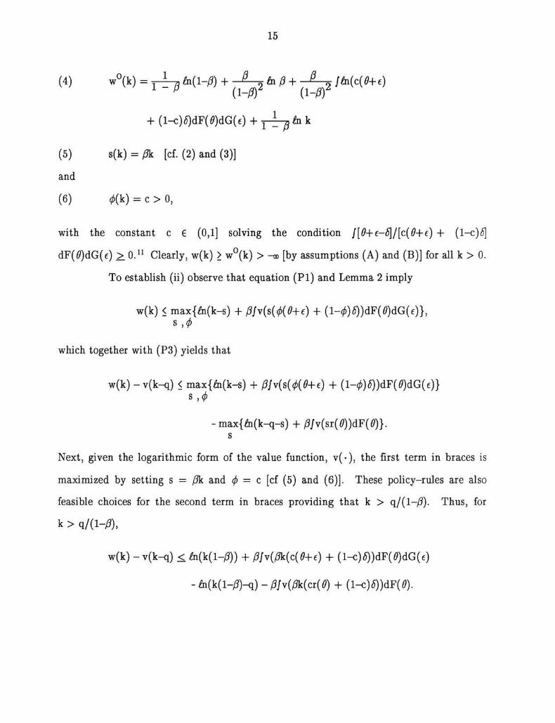
The nonnegative sign of the above expression obtains since the random variable r( 0) =

7max(5,0) stochastically dominates 0 in the second-order sense by assumption ( C ) . 1 0

Final ly , to start the induction hypothesis, let w°(k) = 1/(1-/3) ta(l-0) + P/{l-P)2 to. 0 +

1/(1-/3) A i k. Then, v(k) - w°(k) = p-y/(l-p)2 Jin max(£,0)dF(0) > 0. •

The extent of participation in the exchange network is now easily

characterized. Consider some arbitrary set of agents for whom it was not in their

individual interests to engage in trade with the intermediary up unti l the current period t.

(This set of agents could be all or none of the actors in the economy.) Each of these

individuals must now decide on whether or not to join the market sector. Given that the

cost of accessing the intermediary is lump-sum, it seems likely that agents with a capital

stock fall ing below some minimal level k > 0 wi l l remain outside of the exchange network

while those having an endowment exceeding some upper threshold level k~ > k wi l l join.

Lemma 3: There exist k and k~, with 0 < k < k~, such that

v ( k t - q ) < w(k t ) for 0 < k t < k, and v(k t ~q) > w(k t ) for k t > k~.

Proof: Since both w(k) and v(k) are continuous functions in k, it is enough to

demonstrate that (i) l i m [w(k) - v(k-q)]> 0 and (ii) l im[w(k) - v(k-q)] < 0. To show k-tq k-t C D

(i), note on the one hand that from equation (2) l i m v(k-q) = -co. On the other hand, k-tq

though, it is feasible never to join the coalition and pursue the dynamic-program shown

below:

(P4) w°(k) = max{Ai(k-s) + /?/w°(s(tf>(0+e) + ( l -0 )£) )dF(0)dG(e) } . s , 0

It is easy to show that the value function w°(k) and the policy-rules s = s(k) and <p =

(j)(k) have the following simple forms:

15

1 p {i-PY (i-P)2

+ (l-c)tf)dF(0)dG(e) + j r ^ - g A i k

(5) s(k) = pk [cf. (2) and (3)]

and

(6) <P(k) = c > 0,

with the constant c 6 (0,1] solving the condition J[0+e-b~\/[c(0+e) + (l-c)<$]

dF(0)dG(e) > 0 . 1 1 Clear ly, w(k) > w°(k) > -m [by assumptions (A) and (B)] for all k > 0.

To establish (ii) observe that equation (P I ) and Lemma 2 imply

w(k) < max{6i (k-s) + pjv(s(<f>(0+e) + ( l -<^ ) )dF(0)dG(e) } , S

which together with (P3) yields that

w(k) - v(k-q) < max{m(k-s) + p}v{s{<t>(0+e) + ( l -0)d))dF(0)dG(e)} s ,<j>

- max{6i (k-q-s) + 0/v(sr(0))dF(0)}. s

Next, given the logarithmic form of the value function, v ( - ) , the first term in braces is

maximized by setting s = pk and <p = c [cf (5) and (6)]. These policy-rules are also

feasible choices for the second term in braces providing that k > q/(l~P). Thus, for

k > q/(l-P),

w(k) - v(k-q) < ia(k(l-0)) + P}v{Pk{c{0+e) + ( l -c)£))dF(0)dG(e)

-in(k(l-PU)-PJv(Pk(a(0) + ( l -c )£) )dF(0) .

16

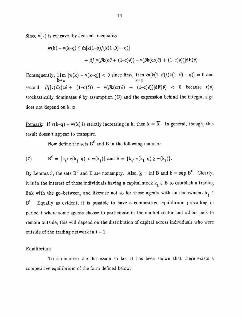
Since v( •) is concave, by Jensen's inequality

w(k) - v(k-q) < Mk( l - / 3 ) / ( k ( l - / ? ) - q)]

+ /?/[v(/5k(c0 + ( l - c ) O ) - v(/?k(cr(0) + (l-c)tf))]dF(0).

Consequently, l i m [w(k) - v(k-q)] < 0 since first, l i m Ai[k( l- /7)/(k( l- /?) - q)] = 0 and k-> C D k-» O D

second, 0/[v(/?k(c0 + (l-c)S)) - v(/7k(cr(0) + (l-c)tf))]dF(0) < 0 because i(0)

stochastically dominates 0 by assumption (C) and the expression behind the integral sign

does not depend on k. o

Remark: If v(k-q) - w(k) is strictly increasing in k, then k = k. In general, though, this

result doesn't appear to transpire.

Now define the sets B and B in the following manner:

(7) B C = {k t : v ( k t - q ) < w ^ ) } and B = v(k t ~q) > w(k t ) } .

By Lemma 3, the sets B c and B are nonempty. Also, k = inf B and k~ = sup B c . Clearly,

it is in the interest of those individuals having a capital stock k . e B to establish a trading

l ink wi th the go-between, and likewise not so for those agents with an endowment k 6

B . Equal ly as evident, it is possible to have a competitive equil ibrium prevailing in

period t where some agents choose to participate in the market sector and others pick to

remain outside; this wil l depend on the distribution of capital across individuals who were

outside of the trading network in t - 1.

Equi l ibr ium

To summarize the discussion so far, it has been shown that there exists a

competitive equil ibrium of the form defined below:

17

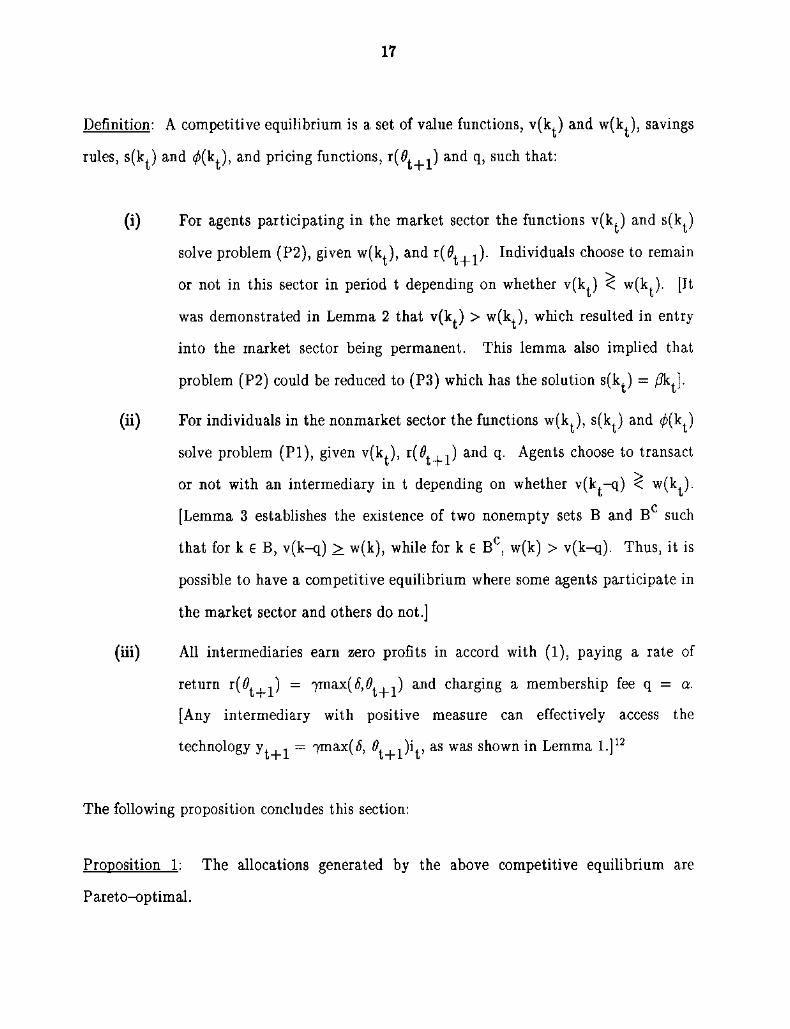
Definit ion: A competitive equil ibrium is a set of value functions, v ( k t ) and w(k t ) , savings

rules, s(k t ) and </>(kt), and pricing functions, r (^^_j) a r>d q, such that:

(i) For agents participating in the market sector the functions v(k^.) and s (k t )

solve problem (P2), given w(k t ) , and Individuals choose to remain

or not in this sector in period t depending on whether v(k^) ^ w(k^). [It

was demonstrated in Lemma 2 that v(k^) > w(k t ) , which resulted in entry

into the market sector being permanent. This lemma also implied that

problem (P2) could be reduced to (P3) which has the solution s (k t ) = /TkJ.

(ii) For individuals in the nonmarket sector the functions w(k t ) , s (k t ) and 0 (k t )

solve problem (P I ) , given v ( k t ) , r ( # t + 1 ) and q. Agents choose to transact

or not with an intermediary in t depending on whether v(k t ~q) < w(k^).

[Lemma 3 establishes the existence of two nonempty sets B and B such

that for k 6 B, v(k-q) > w(k), while for k 6 B c , w(k) > v(k-q) . Thus, it is

possible to have a competitive equil ibrium where some agents participate in

the market sector and others do not.]

(iii) A l l intermediaries earn zero profits in accord with (1), paying a rate of

return r ( # t + 1 ) = jma,x(6,0i+^) and charging a membership fee q = a.

[Any intermediary with positive measure can effectively access the

technology yt_|_^ = 7max(£, ^^.j)i j> a s w a s shown in Lemma 1.]

The following proposition concludes this section:

112

Proposit ion 1: The allocations generated by the above competitive equil ibrium are

Pareto-opt imal .

18

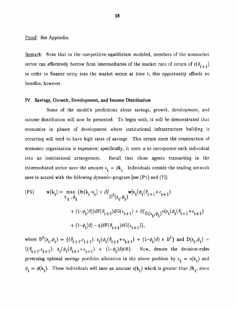
Proof: See Appendix.

Remark: Note that in the competitive equil ibrium modeled, members of the nonmarket

sector can effectively borrow from intermediaries of the market rate of return of r (# t + ^ )

in order to finance entry into the market sector at time t; this opportunity affords no

benefits, however.

IV . Savings, Growth, Development, and Income Distribution

Some of the model's predictions about savings, growth, development, and

income distr ibution wi l l now be presented. To begin wi th, it wi l l be demonstrated that

economies in phases of development where institutional infrastructure building is

occurring wi l l tend to have high rates of savings. This occurs since the construction of

economic organization is expensive; specifically, it costs a to incorporate each individual

into an insti tut ional arrangement. Recall that those agents transacting in the

intermediated sector save the amount s . = pk^. Individuals outside the trading network

save in accord with the following dynamic-program [see (P I ) and (7)]:

(P5) w (k t ) = max {la{k^) + fij ^ ( 0 +e ) s t ,<pt D ( s t , 0 t )

+ ( l - 0 t ) * ) ) d F ( 0 t + 1 ) d G ( e t + 1 ) + / ? / D ( S M ) v ( 8 T ( ^ T ( ^ T + 1 + e t + 1 )

+ ( l - 0 t ) « 5 ) - q ) d F ( < ? t + 1 ) d G ( £ t + 1 ) } ,

where D c ( s t , 0 t ) = { ( * t + 1 , e t + 1 ) : " t W t + l + S + l ) + ( 1 _ < ^ ) G B ° > a n d D ( s t ' < V =

{ ( ^ t+ l ' e t+ l ^ : s t ^ t ^ t + l + e t + l ) + i^-^)^)^}- Now, denote the decision-rules

governing optimal savings portfolio allocation in the above problem by s^ = s(k^) and

0 t = </>(kt). These individuals wi l l save an amount s (k t ) which is greater than 0k^, since

19

they expect at some future date to incur the lump-sum cost q of developing a l ink with

the exchange system.

Proposit ion 2: s (k t ) > pk^.

Proof: The proof proceeds by induction. Consider the sequence of functions {w*} J _ Q and

{ S ^ } " _ Q generated from the mapping = T w ^ - , wi th the operator T defined by

(8) T w J " 1 = max fla(k-J~ 1)+0J „ w^~1(s^1{4>{O+e)+{l-(f>)6))dF(0)dG{e) s J - l 1 D M )

+ ^ D ( s ^ v ( s J - V ( < ? + e ) + ( l - ^ ) t f ) - q ) d F ( ^ d G ( c ) } .

Observe that the mapping T depends upon the values for s and <p specified by (P5), that

is, here s and <f) are being taken as exogenously given constants invariant with the value of

k in (8). Given the fixity of the sets D (s,tp) and D(s,0), the operator T maps concave

functions into str ict ly concave ones. The efficiency condition governing the optimal

choice of s^~ in the above mapping is shown below:

(9) ^ 4 = /?/ c ( W + O + U - f l W V ^(0+6)+(l-0)<5))dF(0)dG(6) k - s J 1 D c (s ,0) k

It is easy to show that the operator T is a contraction whose fixed point defined

by w = Tw is characterized by (P5 ) . 1 3 Thus given any ini t ial function w ° , l i m w^ = w j-»oo

and l i m s- = s. Now, first it wi l l be demonstrated that i f w^ > w£ 1 then s-* > s 1 and J-.00

wk~*~^ > w l c ' Second, to start the induction hypothesis, a concave w ° wil l be chosen so

that w£ > w£ and s°(k) > pk. Consequently, s(k) = l i m s^(k) > pk since s\k) is an

increasing sequence.

20

Assume that > . F rom (8), the first-order condition governing the

optimal choice of s is

— c, X M ^ 0 + ( i - M w j [ ( s J ( D (s,0)

+ # D M ) M * + £ ) + (l-^)^)v k(sJ(0(<?+e) + ( l - 0 ) £ H ) d F ( 0 ) d G ( e ) .

(10) - ^ — r = /?/ _ M0+c) + (1-0) W ( S J ( 0 ( 0 + e ) + (l-0)«5))dF(0)dG(e) k - s J D c (s ,0 ) K

By comparing (10) with (9), observe that i f = s ^ then the r ight-hand side of the

above expression would exceed the left-hand side since w^ > w^ . To restore equality s

must be increased, since the r ight-hand side is decreasing in s-' while the left-hand side is

increasing given that w^ and v are both strictly concave. Next, note that by the envelope

theorem

w j + i L k " Z V k - s J

(recall that s and <p are being held constant). Thus, if > then w ^ ^ > w j | -

F ina l ly , let w ° be specified as in (4) and consequently be concave. Then using

(2), (4), and (9) the efficiency condition governing the optimal choice of s° can be written

as

«H0+e) +(1-4)6 1 = /?/ „ dF(0)dG(e)

k - s° D c ( s , 0 ) ( l - / ? ) [ s ° ( 0 ( 0 + e ) + {1-4)6)]

0(0+e) + (1 -0 ) 6 + Pint, *\ n dF(0)dG(e).

P J » M ) [ { l - m ° { < K 0 + e ) + ( l - 0 ) < 5 ) - q ]

It is easy to see that s°(k) > pk, since when s°(k) = pk the r ight-hand side of this

expression (which is decreasing in s°) exceeds the left-hand side (which is increasing in

s°). Last, it immediately follows that w£ > w£ as

21

1 1 ^ 1 o „ w k = 7 T 7 > ( l = ^ = W k - D

Agents transacting with an intermediary save the amount s t = pk^ and earn a

per unit rate of return of r ( ^ t + ^ ) = VR&xiWt+il o n t m s savings. Consequently, their

wealth grows at the expected rate E [ k t + 1 / k t ] = $ 7 / m a x ( £ , 0 t + 1 ) d F ( 0 t + 1 ) > 1 [by t

assumptions (A) and (C)]. Individuals outside of the exchange network save s t = s (k t ) >

/3k t, earning a rate of return of 0 ( k t ) ( 0 t + 1 + e t + 1 ) + (l-tf)(k^))6. Thus, they accumulate

wealth at the expected rate E [ k t + 1 / k t ] = ( s ( k t ) / k t ) [ 0 ( k t ) / 0 t + 1 d F ( 0 t + 1 ) + (l-0(k t))<5] t

> 1 [by (A) , and Proposit ion 2]. It's unclear whose wealth is growing faster on average.

Whi le on the one hand agents in autarky face an inferior distribution of returns on their

investments, on the other they tend to save more.

It seems reasonable to suspect, though, that very poor agents have a low

savings rate. That is, for the very poor s (k t ) ~ pk^. If so, then poor individuals wil l

accumulate wealth at approximately the expected rate P[<l>^l O^-^dF(O^y) + (l-<^)<5] <

PJy m a x ( £ , 0 t + 1 ) d F ( # t + 1 ) . Consequently, there wi l l be an increase in inequality across

the very rich and very poor segments of the population. The rationale underlying this

conjecture is that very poor agents are l ikely to remain outside of the intermediated sector

for some time to come and consequently are heavily discounting the future cost of

developing a l ink with the exchange network. Addi t ional ly , from (P4) it is known that in

circumstances where an agent wi l l never transact with the go-between the amount s t —

Pk^ is saved.

Proposit ion 3: For all e > 0 there exists a k such that

(a) sup | s ( k ) / k - / ? | < e and (b) sup |0 (k ) - c | < e.

ke[0,R] ke[0,k]

22

Proof: Consider the dynamic-programs (P5) and (P4) defining the value functions w(k)

and w° (k ) , respectively, and the associated policy-rules s(k), 0(k), and pk, c. Since the

value function connected with problem (P4) is strictly concave, it suffices to demonstrate

that

(11) l i m

R-.0

sup | w ( k ) - w ° ( k ) | = 0. ke[0,R]

It wi l l be shown first that (11) holds and second that this condition implies the assertion

made in the proposition.

Note that under program (P5) the minimal capital stock for which i t is

potentially profitable to join the exchange network is k. Let the current period be t and

consider an indiv idual who has an ini t ial endowment of capital k t = k and is saving in line

with this program. Now define P t + j ( k ' ; k ) as the probabil i ty that under the savings plan

s t = s(k t ) and portfolio rule 0 t = 0(k t ) the agent's capital stock wi l l exceed k for the first

time at t + j but then have a value less k ' ; that is, more formally, P . .(k ' ;k) =

p r o b [ k ^ j < k ' , kj._j_j > k, and k ^ j < k for 0 < i < j - l ] with k ^ j being generated by the

law of motion k t + j = [<K\+y_i)(Ot+j+et+j) + ( 1 - « ^ ( k

t + j _ i ) ) < 5 ] s ( k

t + j _ i ) - T h e s a v i n g s

plan s^ = s(k^) and portfolio rule <p^ = (j>(k^) are also feasible for an individual following

the other program (P4). Note that while implementing this scheme is clearly suboptimal

for (P4) it wi l l yield the same time path of momentary ut i l i ty as (P5) for the duration of

time that the agent remains outside of the intermediated sector under the latter program.

Thus,

C D - C D

(12) w ( k ) - w ° ( k ) < .g^J [ v ( k ' ) - w ° ( k O ] d P (k ' ;k ) k

[recalling that v ( k ' ) > w(k ' ) by Lemma 2].

23

Next, from (2) and (4) it is known that

v (k ' ) - w ° ( k ' ) = [/6i 7max(<$,0)dF(0) - / Ai[c(0+e)

+ (l-c)<5]dF(0)dG(e)] = T > 0,

implying

w(k) - w°(k) < T - 1 ^ / d P t + j ( k ' ; k ) = T E ^ P t + j ( k ) , k j—1

where P ^ j ( k ) = / ^ d P ^ j ( k ' ; k ) is the marginal probability of crossing the threshold level

of capital k for the first t ime at t + j . Alternatively, consider the situation where capital

evolves according to the law of motion k ^ = n | = 1 max[6 , (0 t + j+e t + , j ) ] k t and define

Q. , -(k ' ,k) as the probabil i ty the threshold level of capital k wi l l be crossed for the first

t ime at t + j and have a value no greater than k' . Therefore, Q ._j_-(k) = / ^ d Q ^ ^ k ' , k )

represents the marginal probability of crossing k for the first time at t + j . Clear ly, this

alternative generating process leads to the threshold level of the capital stock being passed

for the first time at an earlier date. It follows that the distribution of the P . , 4(k)'s

stochastically dominates the distribution of the Q. , ;(k) 's in the first order sense, or that * • J

m m : S , P , , .(k) < i S 1 Q . , ;(k) for all m. Since is a decreasing function in j this impl ies 1 4

J — * I T J J—J- i - r j

w(k) - w°(k) < T fi^t+fk) < T .l^Qt+.(k).

Now given any e, T > 0 a sufficiently small value for k, denoted by k(e,T), can

T be chosen so that . E . Q . .(k) < e for all k e [0,k(e,T)l. Therefore

T • OD • pT[e(l-pT) + PT] (13) sup | w ( k ) - w ° ( k ) | i J e - ^ + r £ 0< ri-™ .

k6[0,k(6,T)] J = T + 1

Since this can be done for any e and T , the right-hand side of (13) can be made arbitrari ly

24

t iny by choosing a small e and large T . The desired result (11) now immediately obtains

by lett ing e -» 0 and T -»oo in a manner such that k(e,T) -» 0.

It remains to establish that (11) implies the assertion made in the proposition.

Suppose that (a) is false. Then there exists some e > 0 such that for all 8, k(5) > 0 there

is a k G (0,k(<5)] for which |s(k) /k - P\ > e but s u p x ^ g j ^ ^ j |w(x) - w ° ( x ) | < 6. Let

s(k) = s(k)/k and A = m i n ^ ^ [ l / ( l - x ) 2 + (/3/(l-/3))/x 2] > 0. Now choose k such that

(i) sup k f ^Q K j | w ( k ) - w ° ( k ) | < A / 4 e 2 and (ii) k < k/(0+e). Note (ii) implies that

[<p{0+e) + (l-</>)g\sk G B c with probabil i ty one. Therefore, for k € (0,k],

w(k) = max {> ( ( l - s ) k ) + pj w(sk( <p{0+e) + ( l -0)5))dF(0)dG(e)} s ,<p

< max{^n(( l -s)k) + /?/w°(sk(c(0+e) + ( l ^ )5) )dF(0)dG(e) } + j e 2 , s

using (i) and the fact that setting <p = c is opt imal for w° . Taking a second-order Taylor

expansion of the term in braces [using (4)] around the point s = P, while noting first that

at s = 0 this term equals w°(k) and second that its first derivative at s = p is zero, yields

the result

w ( k ) < w ° ( k ) - 4 ( M ) 2 + ^ 2

The constant A represents the lower bound on the absolute value of the second derivative

of the expression in braces with respect to s. Suppose for some k G (0,k] that | s(k) - P\

> e. Then for this k, w(k) < w°(k) . This is the desired contradiction, since by

construction w(k) > w°(k) for all k > 0. F inal ly , (b) can be proved by similar

argument. •

To reiterate, Proposit ion 3 implies that the difference in relative wealth levels

between members of the intermediated sector and the very poor wi l l widen over time.

This result obtains since both groups have the same savings rate while the former face a

better distr ibution of returns on their investments.

25

Some of the long-run properties of the developed model wi l l now be presented.

To begin wi th, agents in the less-developed sector of the economy accumulate wealth

according to

k t + i = W W + i + W + ( M * k t ) ) * | s ( k t ) .

Now define ^ k ' j k ) as the law of motion, in cumulative distr ibution function form,

governing the evolution of the capital stock that is implied by the above equation. Thus,

^>(k';k) = p r o b [ k t ^ < k ' | k ^ = k]. Note that those agents entering t with a k^ e B wil l

join the intermediated sector, it not being worthwhile for the rest ( k t 6 B ) to establish a

link at that time. Therefore, ^ (k ' ; k ) = / d ^ z j k ) represents the probabi l i ty that B c n (0 , k ' ]

an agent residing in period t in the less-developed sector of the economy with k units of

capital wi l l remain in this sector in t + 1 with a capital stock in value no greater than k' .

Next, let H Q (k ) represent the economy's ini t ial time zero distribution of capital

over people so that H Q : -»[0,1]. The ini t ial sizes of the developed and less—developed

sectors of the economy wi l l therefore be / g d H Q ( k ) and 1 - / g d H Q ( k ) . Consequently, the

distribution function governing the allocation of capital across individuals in the less-

developed sector of the economy in period one wi l l be given by H^ (k ' ) =

/ $ k ' ; k ) d H (k). In general,

B c

II t + 1 ( k ' ) = / # k ' ; k ) d H t ( k ) , o

where H t ^_ j (k ' ) measures the expected size of the population in period t who are outside

of the intermediated sector and have a capital stock k ^ j < k ' . 1 5 Note that by

construction the H ^ ^ ' s have all of their mass on B . Since in any given period t+1 no

agent outside of the developed sector has a capital stock k t _^ > k~ (Lemma 3), it follows

that the expected t + 1 size of the less-developed sector is H t + 1 ( k~ ) . Given the assumed

growth in the economy, l i m H t + 1 ( k ~ ) = 0 (i.e., the less-developed sector fades away) . 1 6

t-»co

26

Final ly , in any given period t those agents in the less-developed sector of the

economy realize a rate of return of [^(k t _^)(^+c t ) + (1—^(k t_j))5] on their investments

while those in the developed part obtain the yield 7max(£,0 t). Therefore, for any given

realization of the aggregate shock 0^ = 0 the expected return earned across individuals,

denoted by R t ( 0 ) , is

k" R t (0 ) = J[4(k)9 + ( l - t f k M d H ^ k ) + [1 - H w ( l ) ] 7max(8,0).

Clearly, as the future t ime horizon is extended, R t (0 ) converges (although perhaps

nonmonotonically) to the best technologically feasible expected return possible,

7max(<5,0), conditional on the aggregate state-of-the-world.

Proposit ion 4: l i m sup|R,(<?) - 7max(<5,0)| = 0. t~* w 0

Furthermore, note that individuals outside and inside of the organized sector of

the economy save the amounts s^ = s(k^.) and s^ = pk^, respectively. Consequently, as

the less-developed sector atrophies, larger numbers of agents are accumulating wealth at

the expected rate pjE[max(6,0)]. Thus, asymptotically all agents' wealth wi l l be growing

at the same rate and a stable distribution of relative wealth levels, say as measured by a

Lorenz curve, wi l l a t ta in . 1 7 The economy's expected growth rate converges (though 2

nonmonotonically) to P jE[max( 6,0)] with variance {Pi) var(max(<5,0)).

F inal ly , observe if a nation's in i t ia l distr ibution of capital , H Q , is concentrated

sufficiently close to the origin then its growth factor R^(0) approaches cO + ( l - c ) £ w i t h 2

mean and variance cE[0] + (l-c)6 and c var(0), respectively. Thus, the relationship between a nation's per capita income and its (subsequent) growth is l ikely to be positive

2 2

on average, and if c var(0) > 7 var(max(<5,0)), the relation between per capita income

and the variance of growth wi l l be negative. 1 8 This is i l lustrated in Figure 1. These two

27

predictions of the model carry over to cross sections of countries' per capita incomes and

their growth rates. 1 9

V. Conclusions

Two themes have been prominent in the growth and development literature:

the l ink between economic growth and the distribution of income, and the connection

between financial structure and economic development. Bo th of these issues were

addressed here within the context of a single model. Growth and financial structure were

inextricably l inked. Growth provided the wherewithall to develop financial structure,

while financial structure in turn allowed for higher growth since investment could be more

efficiently undertaken. The model yields a development process consistent, at least, with

casual observation. In the early stages of development where exchange is largely

unorganized, growth is slow. As income levels rise financial structure becomes more

extensive, economic growth more rapid, and income inequality across the rich and poor

widens. In maturi ty an economy has a fully developed financial structure, attains a stable

distr ibution of income across people, and has a higher growth rate than in its infancy.

28

Appendix

It wi l l now be demonstrated that the competitive equi l ibr ium constructed in

Section III is Pareto-opt imal . The discussion is brief, drawing on material presented in

Lucas and Stokey (1983) and Stokey and Lucas with Prescott (1989). The environment

modeled here is more general than that presented in the text. In part icular, imagine that

a contingent claims market operates in the developed sector, wi th addit ional separate

contingent claims markets functioning at each undeveloped autarkic location. Each

individual in the developed sector has access to three production technologies: y t =

7max(5,c9 t) i t_ 1 , y t = ( 0 t + e

t ) i t _ p a n d y t = Here, as in the text, 0 t represents an

aggregate shock which is common across individual production processes while portrays

an idiosyncratic (or project) specific shock. For subsequent use, denote a person's

1 2 3

investment in these technologies by i^, i^., and i^. Agents in the undeveloped sector can

only access the latter two processes. F inal ly , an individual can move (so to speak) to the

developed sector from an undeveloped one at a fixed cost of a. Note that this structure

allows an agent l iv ing in an undeveloped sector to finance a move by issuing contingent

claims in the developed sector to cover the incurred costs. Individuals in either sector are

also free to insure themselves against both aggregate and idiosyncratic shocks to

production. For subsequent use, let 0* = (0Q,0p---,0 t), 0 ^ = ( ^ t ) ^ t + p - - . ^ t + j ) » f t =

( e p ^ p . . . , ^ ) , and e * + J = ( f t , « t + 1 , - - , e t + j ) , and f and g represent the density functions

associated with F and G . (Note that at this stage of the analysis there is no need to

identify any particular individual in the economy. Therefore, for the time being, let

agents remain anonymous.)

Developed Sector

As was just mentioned, agents in the developed sector are free to participate on

a sector-wide contingent claims market. Define b* + - ' = b * + ^ ( 0 t - 1 , e t - 1 ; 0 * + ^ ,e * + J ) as the

29

amount of contingent claims purchased by an indiv idual at the end of period t - 1 , given

that the event (0^ *,e* "*") has occurred, for consumption in period t+ j contingent on the

realization of (0J| ,€*~^). The market price of a claim to period-t consumption,

conditional on the event (0*,e*), wil l be denoted by p t = p t ( N o w , suppose an agent

in the developed sector enters period t with k^ units of wealth. (Let period-zero

consumption be the numeraire.) This wealth can be used to purchase current

consumption, a portfolio of contingent claims, or to finance physical investments in any or

all of the three production technologies. Thus, the individual 's period-t budget constraint

is

( A . l ) p t c t + S / P s b L i < M L i d « L i j = t + i J t + 1 t + 1 t + 1

.1 + [ P t - / P t + i 7 m a x ( « ^ + 1 ) d 0 t + 1 d € t + 1 ] i t

+ MPt+l t+l+S+l)d*t+ldet+J1? + MPt+^^t+l t+l ^ ptkf

Observe that the individual sells forward the proceeds he earns on any period-t

investment in physical capital. A n agent's savings and investment in period t, s^ and i^,

°° i i i 1 2 3 are given by p t s t = S ^ P j ^ t + l ^ + l ^ t + l a n c * \ = h + *t + i t ' T h e i n c i i v i d u a l wi l l

j= t + l

then enter into t + 1 with k ^ ^ units of wealth, where

, . CD . . .

( A - 2 ) k t + i = h l l i + u / P t + i ) = / P j h i + i d 0 i + i *4+r

It is now easy to see that agents in the market sector solve the dynamic

programming problem shown below:

(P6) v ( k t ) = max{6 i (c t ) + / 3 / v ( k t + 1 ) d F ( ^ + 1 ) d G ( e t + 1 ) } ,

« 1 2 3

subject to the constraint ( A . l ) , with the choice variables being c^, b ^ p i^, i^, and i t ,

and where is given by (A .2 ) . 2 0 The upshot of the implied maximizat ion routine is

the following set of efficiency conditions:

30

( A - 3 ) i = / ? v ' ( k t + 1 ) p t / p t + 1 f ( ^ t + 1 ) g ( e t + 1 )

(A.4) p^ > / P t + i T ^ a x C ^ t + l ^ ^ t + l d e t + l ( w ' t n equality i f > 0)

(A.5) p t ^ / P t + 1 ( 0 t + 1 + e t + 1 ) d 0 t + 1 d c t + 1 (with equality i f i 2 > 0)

and

(A.6) p t ;> /p t_j_j ^0 t_j_j det_|_^ (with equality i f i t > 0).

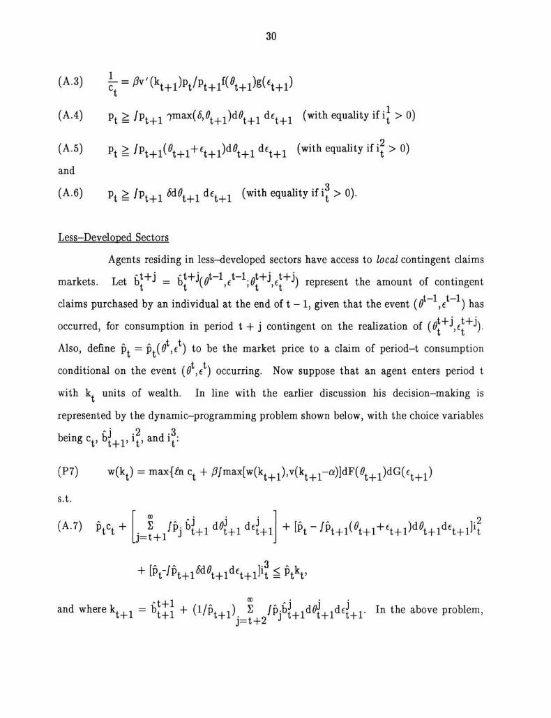
Less-Developed Sectors

Agents residing in less-developed sectors have access to local contingent claims

markets. Let bJ+J = b j + J ( ^ V 1 ; ^ + ^ , e { + J ) represent the amount of contingent

claims purchased by an individual at the end of t - 1, given that the event ( ^ ~ \ e t - 1 ) has

occurred, for consumption in period t + j contingent on the realization of

Also, define p t = p.(0*,e') to be the market price to a claim of period-t consumption

conditional on the event (0 ,e ) occurring. Now suppose that an agent enters period t

with k^ units of wealth. In line with the earlier discussion his decision-making is

represented by the dynamic-programming problem shown below, with the choice variables

•2 . : 3 being c t , b j + 1 > i t , a n d i t :

(P7) w (k t ) = max {& c t + ) 9 / m a x [ w ( k t + 1 ) , v ( k t + 1 - a ) ] d F ( < ? t + 1 ) d G ( c t + 1 )

s.t.

(A.7) p t c t + J / P j b j + 1 d 0 j + 1 d , J + 1 + [ P t - / P t + 1 ( ^ + 1 + ^ + 1 ) d ^ t + 1 d e t + 1 ] i 2

+ [ M p t + l W < ? t + l d e t + \ h ^ P t k t '

• i i CD . . .

and where k t + 1 = b ^ + ( l / p t + 1 ) £ / p j b ^ + 1 d ^ + 1 d 6 ^ + 1 . In the above problem, j= t+2

31

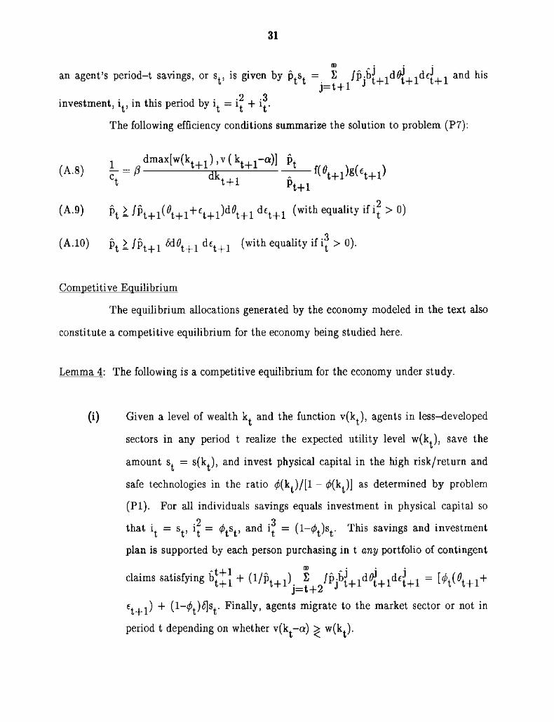
an agent's period-t savings, or s t , is given by p t s t = E / P j ^ t + l ^ + l ^ t + l a n d * " s

j = t + l 2 3

investment, i t , in this period by i^ = i^ + i ..

The following efficiency conditions summarize the solution to problem (P7):

, dmax[w(k. l ) , v ( k . , 1 - a ) ] p t

(A.8) L = 0 t + 1

d k

t + 1 r—^t+iM\+i)

(A.9) p t > / P t + 1 ( ^ t + 1 + c t + 1 ) d ^ t + l d e t + l ( w i t h e c l u a l i t y i f H > °)

(A.10) p t > / p t + 1 <5d^ t + 1 d e t + 1 (with equality i f i j > 0).

Competi t ive Equi l ibr ium

The equil ibrium allocations generated by the economy modeled in the text also

constitute a competitive equil ibrium for the economy being studied here.

Lemma 4: The following is a competitive equil ibrium for the economy under study.

(i) Given a level of wealth k t and the function v ( k t ) , agents in less-developed

sectors in any period t realize the expected ut i l i ty level w(k^.), save the

amount s^ = s(k^), and invest physical capital in the high r isk/return and

safe technologies in the ratio </>(kt)/[l - </>(kt)] as determined by problem

(PI ) . For all individuals savings equals investment in physical capital so

2 3

that i^ = s^, i^ = </>tst, and i t = (l-tp^s^. This savings and investment

plan is supported by each person purchasing in t any portfolio of contingent

claims satisfying b t + 1 + ( l / p t + 1 ) J / P j 6 t + l d ^ + l d c t + l = W t + 1 +

j— t+z

e t^_j) + (l-0 t)<$]s t. F inal ly , agents migrate to the market sector or not in

period t depending on whether v (k t ~a) ^ w(k t ) .

32

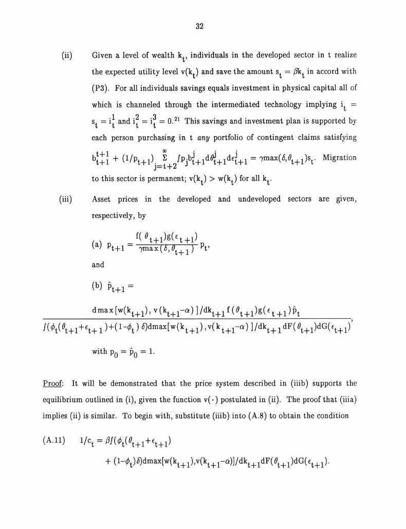
(ii) Given a level of wealth k^, individuals in the developed sector in t realize

the expected ut i l i ty level v(k^) and save the amount s . = (3k^ in accord with

(P3). For all individuals savings equals investment in physical capital all of

which is channeled through the intermediated technology imply ing i t =

1 2 3

s. = i. and i = i, = 0 . 2 1 This savings and investment plan is supported by

each person purchasing in t any portfolio of contingent claims satisfying b{+"l + ( 1 / P t + 1 ) J IVjH+M+M+l = 7 m a x ( M t + 1 ) s t . Migrat ion

J—t+2

to this sector is permanent; v(k^.) > w(k^) for al l k ..

(iii) Asset prices in the developed and undeveloped sectors are given,

respectively, by

. . _ * ( ' t + i ) 8 ( ' t + i ) W p t + l ~ 7 m a x ( i ' , 0 t + 1 ) p t '

and

( b ) Pt+1 =

d m a x [ w ( k t + 1 ) , v ( k t + 1 - a ) ] / d k t + 1 f ( 0 t + 1 ) g ( e t + 1 ) p t

/ ( ^ ( V k + S + i W 1 - ^ ) ^ ™ ^

with p Q = p Q = 1.

Proof: It wi l l be demonstrated that the price system described in (i i ib) supports the

equil ibr ium outlined in (i), given the function v(- ) postulated in (i i). The proof that (iiia)

implies (ii) is similar. To begin wi th, substitute (iiib) into (A.8) to obtain the condition

( A . l l ) l / c t = /W t(* t +l + £t+l)

+ ( l - 0 t ) 5 ) d m a x [ w ( k t + 1 ) , v ( k t + 1 - a ) ] / d k t + 1 d F ( 0 t + 1 ) d G ( 6 t + 1 ) .

33

Now from the allocation rules specified in (i), together with (A.9) , (A.10), and the

definition for k t + p it follows that c t = k t - s t and k ^ j = ( ^ ( ^ t + j + ^ + i ) ~*~ ( ^ ~ ^ t ^ s f

These results, in conjunction with the envelope theorem, allow (A.11) to be rewritten as

_ l _ = / 3 / U(k) ( f l+6) + ( l - f l k ) ) f l d F ( g ) d G ( g )

D c ( s ( k ) , 0 ( k ) ) [ s ^

(A.12) + 0J ffl(*+0 + ( l - W ) * dF(0)dG(«), D(s(k),0(k)) (l-P)[s(k)(<t>(k)(0+e) + (l-<f>(k))6)-a]

where the sets D c (s(k) ,0(k)) and D(s(k),0(k)) are as defined in the text, and time

subscripts have been dropped for convenience.

2

Next, note from (i) that when s^ > 0, i^ = 0 if and only i f <f>^ = 0 and similarly

'u = 0 i f and only i f <f>. - 1. Subtracting (A.10) from (A.9) while making use of (iiib)

yields the result that / ( ( 0 t + 1 + e t + 1 ) - £ ) d m a x [ w ( k t + 1 ) , v ( k t + 1 - a ) ] / d k t + 1 d F ( 0 t + 1 )

d G ( e t + j ) ^ 0, as ^ = 0, 0 < <f>^ < 1, and = 1, respectively. 2 2 The envelope theorem

allows this expression to take the form

( A 13) / \(0+e)-5]dnO)dG(e)

D c(s(k),<Kk)) [s(k)(0(k)(<?+€)+(l-^(k))5)-s(s(k) (<f>(k)(0+e)+(l-m)8))]

+ ^ ( s C k ) , ^ ) ) ( M ) l s ( k ) ( ^ [ H ^ £ ) + ( l - ^ ( k ) ) A ) - a j d I W G ( 0 | °>

as 0 t = 0, 0 < <pt < 1, and (f>i = 1. F inal ly , observe that (A.12) and (A.13) are nothing

but the efficiency conditions for problem (PI ) defining solutions for s(k) and <p(k) and the

associated one for w(k) [see problem (P5)]. •

Pareto-Opt imal i ty

It remains to establish that the valuation equil ibrium modeled above is

Pareto-opt imal . To do this, a bit more notation must be developed. To begin with,

observe that under any interesting allocation rule for the economy, entry into the

34

developed sector wil l be permanent. This must be so since it is feasible for an agent in the

developed sector to duplicate the returns he could realize in autarky by simply operating

the high r isk/return and safe technologies in isolation from others in the sector. Therefore

to conserve notation, attention wi l l be l imited to situations where entry into the

developed sector is permanent. Note that when an individual moves in period t from a

less-developed sector to the developed one, he takes a certain stock of wealth in terms of

goods, to be denoted by k^, with him. Thus, let agent j 's period-t allocation in a

less-developed location be represented by his consumption there, c t ( j ) , investment in

physical capital, ( i t ( j ) , i t ( j ) , i t ( j ) ) , and his transfer of physical goods to the developed

sector, k t ( j ) . Simi lar ly, j 's allocation in the developed sector t is specified by his

~1 ~2 ~3

consumption c^(j), investment in physical capital, ( i ^ ( j ) , i t ( j ) , i t ( j ) ) , and transfer of

wealth to his autarkic is land, & t(j). Whi le this notation has been defined at a general

level, it should be understood that (i) since an individual cannot consume and invest at "1 "2 *3

two locations simultaneously at least one of the vectors [ c t ( j ) , i t ( j ) , i t ( j ) , i t ( j ) ] or 1 ~1 ~9 ~3 ~1 ~2 ~ 3

[ c t ( j ) , i t ( j ) , i t ( j ) , i t ( j ) ] must be identically zero, (ii) if any one of c t ( j ) , i t ( j ) , i t ( j ) , i t ( j ) "1 "2 "3

or k t ( j ) is nonzero then the vector [c j ) , i^( j ) , ! j 1 ( j ) ) i j 1 ( j ) 1 kj 1 ( j ) ] is identically zero for all

h > t since membership in the developed sector is permanent, and (iii) i | ( j ) = k t ( j ) = 0

for all t. Consequently, using the above notation, agent j 's allocation in an economy can

be summarized by

{c t ( j ) , i j ( j ) , i t ( j ) , i?( j ) ,k t ( j ) } t = 0

where

, etc., etc.

Next, for an allocation to be feasible for any less-developed sector (say sector j)

in period t, the following must hold:

c t ( j ) = max c t ( j ) ,c t ( j ) , i t ( j ) = max i t

(j)JJ(J)

35

(A.14) c t ( j ) + + + ic t(j) < (0 t +6 t ( j ) ) i 2 _ 1 ( j ) + fi^Q).

Similar ly, for an allocation to be feasible for the developed sector in t, it must transpire

that

(A.15) / [ c t ( j ) + i ; ( j ) + i t

2 ( j ) + iJ( j ) |dA( j )

< / [ 7 m a x ( M t ) i ; _ 1 ( j ) + ( 0 t + 6 t ^ ^ dA(j),

where I(x) = 1 if x > 0 and I(x) = 0 when x = 0 . 2 3 F inal ly , let an asterisk be attached to

a quantity variable to denote its value in the competitive equi l ibr ium modeled above,

which wi l l be dubbed the star-allocation system.

Proposition 1: The star-allocation system is Pareto-opt imal.

Proof: Consider some alternative allocation system distributing to agent j the assignment

1 2 3

of goods {c t ( j ) , i t ( j ) , i t ( j ) , i t ( j ) ,k t ( j ) } "_Q. It wi l l be shown that i t is impossible for this

allocation scheme to make some set of agents (with positive measure) in the economy

better off without making others worse off. To begin wi th, if agent j strictly prefers the

plan {c t ( j ) , i t

1 ( j ) , i 2 ( j ) , i j ( j ) ,k t ( j ) }^ = 0 to { c j ( j ) , i j 1 ( j ) , i f ( j ) , i f ( j ) , k j ( j ) } ^ = 0 then the first

plan must be more expensive; otherwise j would purchase it under the star-allocation

system. This implies that at least one of the following inequalities must hold strictly:

(A.16) P 0 [ c 0 ( j ) + i 2 ( j ) + i § ( j ) + k 0 ( j ) l + t l ^ P t [ c t ( j ) + i 2 ( j ) + i 3 ( j ) + k t ( j ) d^deJO)

>P0*o(i) + tli/Pt ( ^ t + e t ( J ) ) 1 1 - l ( J ) + , 5 l 1 - l ( J ) l d ^ d e l ( J )

or

36

(A . i7 ) P0[e0(j)+iJ(j)+rg(j)+io(J)l + tIi^tM)+ft(J)+ft(J)+fNd4d€i(J)

> p 0

where 8,Q(J) and §,Q(J) denote agent j 's t ime-zero endowments of goods in the

less-developed and developed sectors, respectively (only one of which may be posi t ive). 2 4

If the agent is indifferent between the two plans then both of these inequalities may hold

weakly.

Now suppose (A. 17) holds strictly for some set of agents with positive measure.

Then integrating both sides of (A. 17) over all agents in the economy yields

p 0 / k ( J ) + 1 J(J) + r ?(J) + ~ a

0 ( J ) - V - i ) + VJ))1 d A <J)

+ J i / P t / l T C t U ) + i}( j) + i j ( j ) + i j ( j ) - T m a x t ^ i f ^ U )

- ( V ^ t ^ l - i ^ - ^ ? - i ( j ) - k

t ( j ) + « i ( k t a ) ) l d A ( j ) d t f i d c i ( j ) > °-

But this leads to the feasibility condition (A.15) being violated at some date t. Similarly,

assume that (A. 16) holds strictly for any individual j . This would lead to the feasibility

condition (A. 14) being violated at some date. Therefore, it is not possible for the

proposed allocation to make some set of agents in the economy better off without making

others worse off. o

Remark: As in discussed in Stokey and Lucas with Prescott (1989), the first welfare

theorem does not depend on any assumptions about technology (such as the absence of

fixed costs).

37

Footnotes

'The evidence that early stages of growth are accompanied by a worsening of

the income distr ibution is by no means clear cut. Korea, for example, grew very fast over

the 1965-85 period, but while income inequality did worsen slightly among rural

households over this period, a bigger improvement took place in the distr ibution of income

among urban households (Dornbush and Park 1987, Table 8).

f o l l o w i n g Townsend (1983a), "the idea that trade links are costly, per se,

seems to be a useful formalism, presumably capturing the cost of bookkeeping, the cost of

enforcement, the cost of monitoring when there is imperfect information, the physical cost

of exchange (transportation), the difficulties of communication, and so on" (p. 259). For

instance, each party to an agreement may have to hire lawyers or accountants to advise

on its details, or pay the cost of install ing communication devices (computers, liaisons, or

transportation terminals), or simply incur the educational expenses involved with learning

new business procedures, etc., etc.

3 T o see this, let £ = Ymax (6,0) and H: (R__ -» [0,1] represent the distribution

function governing £. Note that assumption (C) can now be written as

C D CD C O C O

( C ) / [ l - H ( f l ] d £ = / 7max(8,0)dF(0) > j OdF(O) = / [1 -F(0))d0, 0 0 0 0

where F has been extended to IR + by defining F(0) = 0 for 0 6 [0,0) and F(0) = 1 for

0 G p?,co). For £ to be larger than 0 in the sense of second-order stochastic dominance, it

must happen that / * [F( t ) - H(t)]dt > 0 for all x e K + with strict equality obtaining for

some x (Hadar and Russell 1971, Definit ion 2). To show this, observe the following: (i)

H(t) < F( t ) for 0 < t < 7<5 since H(t) = 0 < F( t ) and (ii) H(t) > F( t ) for all t > j6 since

H(t) = F ( t / i ) > F( t ) . Now consider the expression / * [F( t ) - H(t)]dt. For x < j5 this is

clearly positive since F( t ) > H(t) by (i). For x > 7<S rewrite this expression as / ^ [ F ( t ) -

H(t)]dt + y ^ F ( t ) - H(t)]dt. Here, by (i) and (i i), the first term is positive while the

38

second is negative. But ( C ) guarantees that the first term always dominates since

/ o W ) - H(t)]dt > 0 so that / ^ [ F ( t ) - H(t)]dt > - / ^ [ F ( t ) - H(t)]dt > - / ^ [ F ( t ) -

H(t)]dt.

4 F o r the purpose of taking sums, reindex the (countable) collection of agents in

the set A by the natural numbers.

5 Envis ion each period as consisting of two subintervals. In the first subinterval

production is undertaken. Production can be done at anytime within this

subinterval—some projects can be undertaken early, others can be done late. The

intermediary's tr ial projects are run early, the rest late. Agents who choose not to

transact with an intermediary are indifferent about when to operate their projects within

this subinterval, since they cannot observe at that t ime what is happening to production

elsewhere in the economy. In the second subinterval the output from production is

distributed and agents decide how much to consume currently out of their proceeds and

how much to invest for future consumption.

6 Note here that it is being presumed the intermediary commits himself forever

to the policy of paying the return r(# t) in each period t on any and all deposits made in

t - 1, subject only to the stipulation that the depositor has paid at some time the

once-and-for-a l l fee of q. The possibil ity of default is precluded by assumption. Now,

suppose that for some / . i. , (j)dA(j) > 0 and J x , dA(j) > 0 condition (1) could A t - 1 t _ i A t - 1

become negative with positive probabil ity. Then, with positive probabil i ty, any

intermediary could go bankrupt in the first period of its operation and would have to

default on its obligations to depositors (since the intermediary would owe an infinitely

large amount relative to his start up wealth). This , though, is prohibited. Any agent can

become an intermediary, rather than transact with one, i f it is in his own best interest to

do so. Alternat ively then suppose that r(# t) and q are such that (1) never becomes

negative, and is str ict ly positive with nonzero probabil i ty. Here the intermediary could

39

realize infinite profits in any particular period with positive probabi l i ty, and never realize

any losses, a situation ruled out by the assumption of free entry into the industry.

7In a similar vein, Gertler and Rogoff (1989) assume that the probabil i ty of an

investment project attaining a good return is an increasing function of the amount of

funds invested. This again could provide a rationale for agents to pool funds.

t h r o u g h o u t the analysis, it wi l l be impl ic i t ly assumed that the constraints

s t G [0,k t] and 0 G [0,1] apply, as relevant, to the optimization problems formulated.

9 Prob lem (P2) assumes that agents participating in the intermediated sector

wil l invest all their savings with the go-between. Strict ly speaking, the intermediary

requires the use of only one safe technology and a countable inf ini ty of the high

r isk/return ones. Thus it may seem reasonable to allow some agents to make individual

isolated use of the unneeded technologies so as to economize on the proportional

transactions costs associated with intermediated activi ty. It is easily demonstrated, using

equations (A5) and (A6) in the Appendix, that the following assumption ensures such

options, even if available, would never be executed: (D) For al l 0 G [0,1], J[<fr0 +

(l-0)<5]/[7max(0,£)]dF(0) < 1. Note that this assumption holds automatically when

7 = 1 (i.e., no proportional transactions costs). F inal ly , assumption (C) and (D) can be

guaranteed by imposing the single restriction that E[0]E[1 /(jma,x(6,0))] < 1.

1 0See Hadar and Russell (1977), Theorem 2, for more detai l .

"Some more detail on the derivation of the constant c may be warranted.

Suppose that (4) specifies w°. Then the following conditions govern the solution for 0 in

(P4): (i) }[0+e-8\/[<t>(0+e) + ( l-0)d]dF(0)dG(c) < 0 if 0 = 0, (ii) i f 0 G (0,1),

J[0+e-6]/[<t>{0+e) + (l-0)<§]dF(0)dG(e) = 0, and (iii) J[0+e-6]/[<f>(0+e) +

(l-0)<5]dF(0)dG(e) > 0 if 0 = 1. Clearly, the solution for 0 does not depend on k, i.e.,

0 = c where c is a constant. It is easy to deduce that c $ 0. Evaluat ing (i) at 0 = 0

yields J[0+e-6]/6dF(0)dG(e) > 0, which contradicts assumptions (A) and (B).

40

1 2In competitive equil ibrium the goods markets always clear since, for each

agent, consumption plus physical investment in capital (inclusive of transactions costs)

equals his endowment of output.

1 3 Brief ly , the Euler equation connected with problem (P5) is

1 , , - f f f \4>(k)(0+e) + ( l - ^ k ) ) f ] d F ( g ) d G ( 0

+ ^ D ( s ( k ) , m (i-^lfikll^^tl^llmHJ ^ ( e ) ,

with s(k) denoting the optimal policy function. Now consider the fixed point associated

with the mapping shown by (8). Here the sets D c(s(k),0(k)) and D(s(k),^(k)) are fixed,

as far as the impl ied maximization is concerned. The choice problem underlying this

mapping has the following Euler equation:

1 -pi ^ ( k ) ( 0 + 6 ) + ( l - # k ) ) f l d F ( g ) d G ( Q

k-s(k) D c ( s ( k ) , 0 ( k ) ) [ s ^

+ ik4*M d F ( 0 ) d G ( O ,

+ «D(s(k),0(k)) (l-0)[m(HV(O+e) + (WOO)*) - q]

where s(k) denotes the optimal policy function. Next, examine the solutions for the

policy functions to each of these Euler equations; they are the same, implying s(k) = s(k).

Thus, the fixed point to (8) must be represented by (P5).

1 4See Hadar and Russell (1971), Definit ion 1 and Theorem 1.

1 5 Str ic t ly speaking, the H t functions are not proper cumulative distribution

functions as in general H t(co) < 1. Also, the distribution H t is an expectation conditional

on period-zero information. The actual distr ibution of capital, H^, evolves randomly in

response to the realization of 0^. The period-t state of the less-developed sector is ( 0 t , H t )

while the economy-wide state is a triple made up of 0^, H^, and the distr ibution of capital

at t in the developed sector.

41

1 6 B y Proposit ion 3, s (k t ) > (3k^. Consequently, i t follows that 61 k t > in k Q +

t • %,{ln[(p.(0-+e-) + (l-<p-)6\ + in P}. The r ight-hand side of this expression is a random J J J J J

walk with positive drift, since E[&i(0.(0.+ e.) + (1-0:)*)] + 6 1 P > 0 f o r a 1 1 <f>\ e l 0. 1] b y J J J J J

assumptions (A) and (B) . Thus, k t must become absorbed into the set [k~,co) with

probabil i ty one. For more detail see Feller (1971).

1 7In a somewhat different context, Hart and Prais (1956) present evidence on

the tendency for Lorenz curves to first worsen and then improve over time. 2 2

1 8It is easy to construct examples where c var(0) > 7 var(max(£,0)). As a case

in point, suppose 0 is drawn from the set B = {a.^,a2<$} with a^ < 1 < a 2 - Now ^ *" =

prob[0 = a.^6] so that 1 — 7r = prob[0=a2#]. Recall that E[0] > 8, by assumption (A) ,

which translates here to requiring 7 ^ + ( l -7 r )a 2 > 1. F ina l ly , set e = 0. Given that E[0]

> 6, it was demonstrated in footnote (11) that c 6 (0,1]. F i rs t , consider the case where c 2 2

= 1. Tr iv ia l ly , here c var(0) > 7 var(max(6,0)) since 7 < 1 and var(0) >var(max(6,0)).

Second, consider the situation where c € (0,1). Here the constant c is determined by

condition (ii) in footnote (11), which now reads 7 r (a 1 - l ) / [ ca 1 +( l -c ) ] +

( l - 7 r ) (a 2 - l ) / [ ca 2 +( l - c ) ] = 0, implying c = [7 ra 1 +( l -7 r )a 2 - l ] / [ (a 2 - l ) ( l -a 1 ) ] . Clearly, a j 2

and a 2 can be chosen in a manner which makes c sufficiently close to 7 so that c var(0) > o

7 var(max(<5,0)).

1 9 Some interesting evidence that countries' growth rates have actually tended

to increase over time is reported in Romer (1986). Also, Baumol (1986) presents

(graphically on p. 1080) some data in which it appears that dispersion in growth rates

across countries with similar per capita incomes declines as per capita income rises.

2 0 T h e standard solvency conditions apply to the optimalization problems

presented in the Appendix. The solvency condition associated with (P6) is l i m /pj^_j t-»0D

k t + l d ^ + l d f t + l " 0 -21 Assumption (D), footnote 9, is relevant here.

42

2 2 F o r instance, consider the case when </>t = 0. Here by subtracting (A. 10)

from (A.9) one obtains / p t + 1 ( ^ t + 1 + e t + 1 — ^ ) d ^ t + 1 d e t + 1 < 0. The formula for p t + 1

given in (iiib) then allows this expression to be rewritten as ]((0^^+€^^) - 6)

d m a x [ w ( k t + 1 ) , v ( k t + 1 - a ) ] / d k t + 1 d F ( 0 t + 1 ) d G ( e t + 1 ) < 0, as stated in the text. The

other two cases, 0 < 0 t < 1, and 0 t = 1, can be analyzed in similar fashion.

2 3 Str ic t ly speaking, the feasibility condition (A. 15) is too generous. A n agent

could be transferred to the market sector in t with zero capital, yet the resource cost of

moving would st i l l have to be absorbed. To avoid this problem, one could alternatively

use the indicator function I t( j) which is defined to be unity for those states in period t

when agent j moves, and to be zero otherwise. Note that (A. 15) sti l l holds for the original

formulation of the indicator variable, though, since I(k t( j)) < I t(j)-

2 4 T h e left-hand sides of equations (A. 16) and (A . 17) represent the

present-value of expenditure in the developed and less-developed sectors from the

proposed plan, while the r ight-hand sides show the present-value of income.

43

References

Baumol , W i l l i am J . "Product iv i ty Growth, Convergence, and Welfare: What the

Long-Run Data Show." American Economic Review 76 (December 1986): 1072-85.

Bencivenga, Valer ie R., and Smith, Bruce D. "F inanc ia l Intermediation and Endogenous

Growth. " Unpublished paper, University of Western Ontar io, Department of

Economics, 1988.

Boyd, John H. , and Prescott, Edward C. "F inanc ia l Intermediary-Coal i t ions." Journal

of Economic Theory 38 (Apr i l 1986): 211-32.

Cameron, Rondo. "Banking in the Early Stages of Industrialization: A Study in

Comparative Economic History." New York: Oxford University Press, 1967.

Diamond, Douglas W . "F inancia l Intermediation and Delegated Moni tor ing." Review of

Economic Studies 51 (Apr i l 1984): 393-414.

, and Dybv ig , Phi l l ip H. "Bank Runs, Deposit Insurance, and L iqu id i ty . " Journal

of Political Economy 91 (June 1983): 401-419.

Dornbusch, Rudiger, and Park , Yung Chu l . "Korean Growth Po l icy . " Brookings Papers

on Economic Activity 2 (1987): 389^54 .

Fel ler, W i l l i am. "An Introduction to Probability Theory and Its Applications." New

York : John Wi ley and Sons, Inc., 1971.

Freeman, Scott. "Inside Money, Monetary Contractions, and Welfare." Canadian

Journal of Economics 19 (February 1986): 87-98.

Gert ler, Mark , and Rogoff, Kenneth. "Developing Country Borrowing and Domestic

Wea l th . " Unpublished paper, University of Wisconsin, Department of Economics,

1989.

Goldsmi th, Raymond W . "Financial Structure and Development." New Haven: Ya le

University Press, 1969.

44

Hadar, Josef, and Russel l , W i l l i am R. "Stochastic Dominance and Diversif ication."

Journal of Economic Theory 3, (September 1971): 288-305.

Hart , P . E . , and Prais, S. J . "The Analysis of Business Concentration: A Statistical

Approach." Journal of the Royal Statistical Society, A, 119,(1956): 150-81.

Jung, Woo S. "F inancia l Development and Economic Growth: International Evidence."

Economic Development and Cultural Change 34, (January 1986): 333-46.

Kuznets, Simon. "Economic Growth and Income Equal i ty . " American Economic

Review 45, (March 1955): 1-28.

Lindert, Peter H., and Wi l l iamson, Jeffrey G . "Growth , Equal i ty and History."

Explorations in Economic History 22 (October 1985): 341-77.

Lucas, Robert E. " O n the Mechanics of Economic Development." Journal of Monetary

Economics 22 (July 1988): 3 ^ 2 .

, and Stokey, Nancy L. "Opt imal Fiscal and Monetary Pol icy in an Economy

without Cap i ta l . " Journal of Monetary Economics 12 (July 1983): 55-93.

M c K i n n o n , Ronald I. "Money and Capital in Economic Development." Washington,

D .C. : The Brooking's Institution, 1973.

Paukert, Fel ix. "Income Distr ibut ion at Different Levels of Development: A Survey of

the Evidence." International Labor Review 108 (August-September 1973): 97-125.

Rebelo, Sergio. "Long- run Pol icy Analysis and Long-run Growth . " Unpublished Paper.

Rochester: University of Rochester, Department of Economics, 1987.

Romer, Pau l M . "Increasing Returns and Long-run Growth . " Journal of Political

Economy 94 (October 1986): 1002-37.

Shaw, Edward S. "Financial Deepening in Economic Development." New York: Oxford

University Press, 1973.

Stokey, Nancy L., and Lucas, Robert E . with Prescott, Edward, C . " Recursive Methods

for Economic Dynamics." Cambridge: Harvard University Press, 1989.

45

Summers, Robert; Krav is , Irving B.; and Heston, A lan . "Changes in the Wor ld Income

Distr ibut ion." Journal of Policy Modelling 6 (May 1984): 237-69.

Townsend, Robert M . "Intermediation with Costly Bi lateral Exchange." The Review of

Economic Studies 55 (October 1978): 417-25.

. "Theories of Intermediated Structures." Carnegie-Rochester Conference Series

on Public Policy 18 (Spring 1983a): 221-72.

. "F inancia l Structure and Economic Act iv i ty . " American Economic Review 73

(December 1983b): 895-911.

Wi l l iamson, Stephen D. "Cost ly Monitor ing, Financial Intermediation, and Equi l ibr ium

Credit Rat ion ing." Journal of Monetary Economics 18 (September 1986): 159-79.

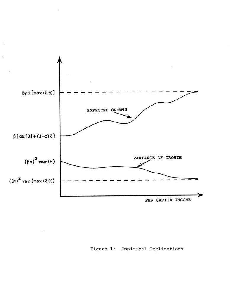
pYE[max(5,8)]

(5{cE[9] + ( l -c )5 }

(pc) var (G)

(py) var (max (5,9))

VARIANCE OP GROWTH

PER CAPITA INCOME

F i g u r e 1 : E m p i r i c a l I m p l i c a t i o n s