The Taylor Rule Application andRelevancy in Current US Economy

Alexander LizzoDr. Hany Guirguis

Finance 402 Federal Reserve CourseTaylor Rule Principle

11/16/2012

Index: Pagenumber

Abstract3

1

The Dual Mandate of the Federal Reserve Board4

Current Issues in the US Economy 4

Taylor Rule as a Monetary Tool 6

The Implications of the Rule 7

Is the Taylor Rule Relevant When the FFR is Zero? 7

Monetary policy targeting FFR 7

Conventional vs. Non-conventional Policy Tools 9

Relevance of Taylor Rule when Targeting FFR – Facts andOpinions 10

Noritaka Kudoh’s argument 11

Athanasios Orphandies argument12

Conclusion – Suggested Further Study13

Appendix 15

Figure 1 15Figure 2 15Figure 3 16Figure 4 16Figure 5 16Figure 6 17 Figure 7 17Figure 8 17Figure 9 18

2

Figure 10 18Figure 11 19Figure 12 19Figure 13 20 Figure 14 20Figure 15 21Figure 16 21

Figure 17 22Figure 18 22Figure 19 23

Abstract

This paper was primarily written to help the reader understand the factors of the Taylor Rule as a Federal Reserve decision making tool. The Taylor Rule is a mathematical model that has been used as a reference for economists to forecast the nominal interest rate – specifically the Federal Funds Rate (FFR). The model has been in use since 1993 after the release of John B Taylor’s proposal. The book documenting the meeting conference where Taylor presented his paper is called Carnegie-Rochester Conference Series on Public Policy, and it explains the model’s effects on different country’s economies. Simply, the rule states that if the inflation rate (measured by the GDP deflator) increases by one percent, then forecasters should adjust the nominal interest rates greater than one percent.

3

The Taylor Rule equation can be used in several stochastic and economic models. However, certain academic scholars haveargued that the Taylor Rule cannot be applied as a monetary tool in the current economic situation after the 2008 recession where the FFR is close to zero because the Taylor Rule principle implies that the FFR should be negative.

This paper will be used in a Federal Reserve Bank Competition to recommend effective monetary tools, and also in a speech to the Manhattan College School of Business. Thepaper does require some basic knowledge of economy at the macro and micro level.

4

The Dual Mandate of the Federal Reserve Board

The Federal Reserve Board’s (aka Fed) primary objective is to promote maximum employment while maintaining price stability which is known as the ‘Dual Mandate.’ The more people employed and working in the economy will generate higher total national output, and thus high Real GDP. Unfortunately, there is a direct relationship that exists between inflation and employment. That is, high rates of employment result in high rates of inflation. To regulate this positively correlated relationship, the Fed must determine the most appropriate strategy of monetary policy using its decision making tools.

The Fed must consider the impacts of monetary policy on boththe long run and short-run employment. The long-run effect of employment and output is determined by unforeseeable future determinants (ie. population growth, new technologies, preferences for saving, etc…) however, monetary policy cannot effect the long-run. Instead, the short term output and employment helps to guide the long-runand reduce variability of fluctuations in prices related to each of thee variable. Stable prices are an essential element required for a sustained robust economy. Monetary policy can be seen to help to stabilize the economy and place it on a path that is consistent with the long-term potential employment goal.

Current Issues in the US Economy

Unemployment is generally considered as the most pressing problem facing the US economy today. Unemployment growth has been increased rapidly since the first quarter of 2008. The figure had grown to approximately 10% at the end of the recession in 2009. Both public and private sector employmenthad decreased by 2.5 million jobs and 5 million jobs,

5

respectively. Only 56% off the adult population was employedduring 2011, compared to 64% employment in 2006 – not considering those ‘not in the labor force’. Unemployment in 2011 was roughly 9%, but only 5% in 2006.1

“Jobs” in fact, were the central theme in the presidential election of 2012. Interestingly, the candidates’ plans to improve employment rates focused on different ways of stabilizing costs (employee medical benefits, business and personal tax rates, etc.)

Price stability in the United States (U.S.) economy is targeted at around 2% annually. Price stability is importantbecause too much inflation increases prices, which distorts efficiently allocating resources. High inflation increases the uncertainty in the prices and makes future decisions more difficult because of the greater risks associated with the volatility. And deflation (the contraction of prices) raises the real burden of nominal debt, and may force marketparticipant to defer spending.

Total and Personal Consumption Expenditure (PCE) deflators that measure inflation have been relatively stable in the past 10 years and have consistently hovered around 2%. And the Federal Open Market Committee expect inflation to maintain it current growth level of 2%.2

The Fed is able to achieve its goals by affecting the flow of credit. Since the onset on the recession the Fed has beenproviding credit easing or economic stimulation by lowering the FFR, which has effectively lowered the cost of credit toits lower bound, zero. The rationale for lowering these interest rates is to make borrowing more attractive, becauserates of return are more likely to surpass the cost of borrowing. More borrowing and more investment should have

1 [see ‘figure 1’ in the appendix]

2 [see figures ‘2’,’3’,’4’ in the appendix]6

the net effect of increasing the aggregate demand in the economy and to persuade banks to look elsewhere for higher rates of return. The Federal Reserve Bank (aka Fed) took immediate actions after the collapse of the banking sector and the housing market in 2008 by cutting all interest rate close to zero to discourage market participants from lendingat the Federal Reserve Rate, and instead invest their cash elsewhere in the market. And now, in 2012, interest rates have continued to remain close to zero.

As a result of the ‘Great Recession’ of 2008, the Real GrossDomestic Product fell by an estimated $850 Billion or 6% below the 2% annual stable Potential GDP line, which some believe could represent a permanent shift in the Real GDP curve. In order for Real GDP to catch up to potential GDP, Real GDP would have to grow at a rate of 3% in the next few years in order to get back on track with potential GDP. And according to Andrea Tambalotti’s and the BEA’s calculations that are based on historical data, the economy has about a 50% chance of recession within one year.3 (Tambalotti, 2012)

As figures ‘5’,’6’,’7’, and ‘8’ in the appendix indicate, The Federal Reserve Bank is dealing with a very delicate situation, which it has decided to handle in a unique way tomaintain its goals.

Maintaining maximum sustainable employment is a difficult task for the Fed because it’s tools for effecting employmentare limited to those associated with the establishment of monetary policy. The Taylor Rule can now be seen to be a very significant means for the Fed and for economists in general, to determine the correct monetary policies and implications for the society. The rule quantifies the effect that the FFR will have on rates of inflation and corresponding GDP.3 [ see figures ‘5’,’6’,’7’,’8’ in the appendix]

7

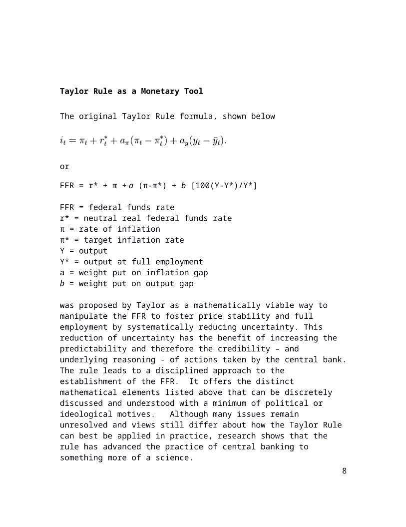
Taylor Rule as a Monetary Tool

The original Taylor Rule formula, shown below

or

FFR = r* + π + a (π-π*) + b [100(Y-Y*)/Y*]

FFR = federal funds rate r* = neutral real federal funds rate π = rate of inflationπ* = target inflation rate Y = outputY* = output at full employmenta = weight put on inflation gapb = weight put on output gap

was proposed by Taylor as a mathematically viable way to manipulate the FFR to foster price stability and full employment by systematically reducing uncertainty. This reduction of uncertainty has the benefit of increasing the predictability and therefore the credibility – and underlying reasoning - of actions taken by the central bank.The rule leads to a disciplined approach to the establishment of the FFR. It offers the distinct mathematical elements listed above that can be discretely discussed and understood with a minimum of political or ideological motives. Although many issues remain unresolved and views still differ about how the Taylor Rule can best be applied in practice, research shows that the rule has advanced the practice of central banking to something more of a science.

8

The rule was derived in part by the examination of the effects of central banks monetary policy and its empirical results.

The Implications of the Rule

The Taylor Rule implies that the nominal interest rate can be varied to limit or curtail the effects of an inflationarytrend and influence the growth of the real GDP. The rule further implies that a high interest rate is required when inflation is considered too high – a “tight” monetary policyand that the interest rate be lowered when inflation is low to stimulate output. The magnitude of the coefficients a and b above represent the relative weight that the economic agency assigns to the inflation and output. In short, the higher the a value, the more significant is the perception of the detriment of inflation. Similarly b is to GDP.

In its simplest terms, the Taylor Rule is a recipe for modifying the rate of inflation to cultivate sustainable growth of the GDP while maintaining stable prices for goods and services.

9

Is the Taylor Rule Relevant When the FFR is Zero?

On August 22, 2012 Ben Bernanke -- president of the Federal Reserve -- wrote a letter to Congressman Darrel Issa . The letter contained a series of questions about the state of the economy. One of the questions posed in the letter was: should the Federal Reserve consider re-adopting the Taylor Rule to stabilize monetary policy? This is an acknowledgement that the Taylor Rule is imperfect and ineffective in an economy where interest rates are close to zero. The elements of the Taylor Rule are clear enough. Maintaining near zero interest rates should have spurred economic growth by spurring investment – to date, this has not been the case. (Bernanke, 2012)

Monetary policy targeting FFR

The Fed has three main traditional policy tools to try to stimulate the economy. The first and primary tool is called the Federal Funds Rate (FFR), which is the rate at which banks can borrow and lend reserves in the federal funds market, basically it the rate at which banks can borrow fromeach other through the Fed. The Fed sets a target/nominal rate for the FFR, and then it will determine the level reserve requirement, so that the Fed can reach its target for demand. The Taylor Rule has been useful in the past for helping to predict the results of specific adjustments to the FFR.

The second conventional monetary policy is the reserve requirement. This is used to determine the amount of money

10

that commercial banks must hold inside the Federal Reserve Bank. When the reserve requirement ratio is increased the credit that the banks are able to issue decreases. The Fed has the ability to adjust reserves and target an ideal FFR through the open market operations, which is the purchase and sale of government securities on the secondary market. The policy operating target is set by the Federal Open Market committee (FOMC), which is composed of FRB chairman, NY Fed president, and 12 voting members. A purchase adds reserves to the banking system, whereas a sale will drain reserves from the banking system.

The final conventional tool is known as the discount window.This is the rate at which banks will receive from the Fed. An increase in the discount rate tightens monetary policy, and a decrease in the discount rate loosens monetary policy.

At the onset of the crisis in 2007 the Fed began implementing a loosening policy, which decreased the nominalFFR. The FFR is considered the risk-free rate and market participants determine their interest rates based on this risk-free rate. In the current policy environment the FFR isclose to zero, so there is obviously no potential way the Fed can make further reductions. The FOMC has stated “…exceptionally low levels for the federal funds rate for an extended period.” (June 22, 2011 FOMC statement) and “… are likely to warrant exceptionally low levels for the federal funds rate at least through mid-2013.” (August 9, 2011 FOMC statement)4.”

These tools affect the economy through the monetary transmission mechanism. Policies primarily affect the structure of nominal interest rates by influencing aggregatedemand through different channels.5

4 [ See figure 9: Federal Funds Rate Target and the Taylor Rule]

5 [ see figure 10 : monetary transmission: FFR target set freely, in theappendix]

11

However, the transmission mechanism broke during the financial crisis. 6 Although the FFR was reduced during thistime term lending was impaired and credit spreads widened. These problems were a reflection of severe strains at markets and financial institutions due to the uncertainty for each institution. That is, they were caused by uncertainty of the potential of future investments and ratesof return, not of existent rates. That is – the strains resulted from limited amount of investors willing to invest moneys, because of future uncertainties – such as the cost of medical programs, taxes, etc previously discussed.

Conventional vs. Non conventional Policy Tools

In effect, the Federal Reserve Banks as well as the FOMC hadlowered interest rates so low that their policy tools – and models such as the Taylor Rule – were ineffective in determining a course of action. Therefore, the Fed had tostart using new policy tools after 2008.7 Beginning in October 2008, banks are permanently required to pay intereston bank reserves. Second the Fed is temporarily providing lending and credit to provide liquidity to the financial system and support the extension of credit. This will createlending facilities for the banks and financial intermediaries and also create funding facilities for other market participants. And the Fed has been providing credit easing programs. Although some of these facilities will be restricted by the Dobb-Frank Act at some time in the future.The third non-conventional policy tool is the long-term asset purchases, which should influence the long-term rates

6 [see figure 11: monetary transmission: broken transmission mechanism,in the appendix]

7 [See figure 12: traditional vs. non-traditional, in the appendix]12

and reduce the risk in these markets (ie the mortgage markets.)     In addition the Fed has been purchasing large amounts of security assets. The buy back program is known as the Large Scale Asset Purchase (LSAP) and it serves as a commitment device, as well as, directing the movement of long rates.8 According to the minutes of the September FOMC meeting the Fed will offer maturity extension program and the Mortgage Back Security reinvestment (MBS) 9

The Fed started rounds of major accommodations in order to stimulate the economy, which became known as Quantative Easing (1-3) and Operation Twist. The first round, QE1, was a 1.25 trillion dollar purchase of MBS; QE 2 was a 600 billion dollar purchase of Treasuries; Operation Twist was an attempt to shift the maturity and flatten the yield curveof Treasuries buy purchasing long-term and sell short-term Treasuries; and finally QE 3 is an open ended purchase program of 40 billion dollars worth of MBS.

Now the Fed is facing a new challenge in 2012 because the monetary transmission mechanism is broken.10 The Fed is resorting to a forward guidance policy. The Fed is communicating its forward plans in order to reduce the amount of uncertainty in the markets, and give market participants more knowledge for forecasting.

Lowering the FFR has increased the supply of reserve and reduced the market rate, which has changed the composition and the size of the Federal Reserve’s balance sheet.11 The balance sheet on the asset side is now composed of new loans8 [see figure 13: short and long term treasury yields]

9 [see figure 14 monetary transmission: FFR Near Zero]

10 [see figure 15: addressing the broken transmission mechanism in theappendix]

13

and portfolio under various credit programs. Also the Fed isholding more long-term treasuries and agency MBS. Under the liabilities section excess reserves have increased greatly. This has created a new challenge of how to manage an expanded balance sheet for decision makers at the Fed.12 William Dudley’s (President of the NYC FRB) forecasted predictions indicate that the Taylor Rule adjusted to include the balance sheet adjustment will allow the Federal Funds rate to liftoff a year earlier than the unadjusted equation. 13

The goal of the FOMC’s is to stabilize economic activity andinflation. The economic operates with lag so, the goal for interest rate policy is a reflection of the FOMC’s assessment of current economic condition and likely evolution of output and inflation. One of the convenient benchmarks for policy stance is the “Taylor Rule.”

Relevance of Taylor Rule when Targeting FFR – Facts and Opinions   The Taylor Rule is a simple policy tool that is dependent ona complicated relationship between monetary policy and economic outcomes. If the Fed was able to stay on course with its consistent 2%growth index, then this relatively simple policy rule would not require re-examination. However, that is not the case, the relationship between monetary policy decisions and the real economy is variable. William Dudley of the Federal Reserve Bank of New York claims “However, if the linkage between monetary policy and 11 [See figure 16: Excess reserves ]

12 [see figure 17: Federal Reserve Balance sheet: assets and liabilities]

13 [see figure 18: Taylor Rule 1999 with and without balance sheet adjustments]

14

the real economy is more variable, as I believe it is, then an approach that is more pragmatic and updates the policy setting in a clear and systematic manner based upon what theFOMC learns over time will be more effective.” (Dudley, 2012)

Members of the FOMC argue what weights should be applied to the expected inflation versus deviations from output. Policymakers make decisions based on their cost analysis of deviations from the dual objective and the structure of the Taylor Rule.  “This debate can be summed up by looking at the two most well-known versions of the Taylor Rule—the original version put forward by Mr. Taylor, which is commonly referred to as Taylor 1993, and a later version updated by other economiststhat Mr. Taylor has discussed but does not endorse, which isreferred to as Taylor 1999.  Taylor 1999 puts more weight ondeviations of output from potential than Taylor 1993.  Thus,Taylor 1999 would lead to a later liftoff of the federal funds rate as the economy returns to full employment.

Which set of weights is better is a matter of judgment. JohnTaylor prefers Taylor 1993.  My own thinking, when translated into Taylor Rule terms, favors the weights in theTaylor 1999 formulation.14  I believe that Taylor 1999 is likely to perform better in achieving the Federal Reserve’s dual mandate objectives.  Compared with Taylor 1993 it can achieve significantly greater stability in employment without sacrificing the medium-term inflation objective or significantly increasing the variability of inflation outcomes. ”  (Dudley, 2012)

Noritaka Kudoh’s argument:

Noritaka Kudoh created a model in a steady state equilibrium14 [Figure 19: Taylor Rule 1999 with Alternative Real Rate Assumptions]

15

and tested monetary policy and fiscal policy by applying theCobb-Douglas model.

“The Taylor Rule itself generates a negative relationship between output and inflation. As a result, under an active monetary policy, an increase in government spending translates into a higher nominal interest rate and lower capital and output. The study found that an increase in government spending requires a increase in either direct taxrevenue, the seigniorage, or the revenue from bonds. According to the monetary policy tool the Fisher Equation implies an increase in inflation reduces capital accumulation if and only if monetary policy is active. Thus,under and active monetary policy, an increase in the government’s needs for revenue increases the inflation rate,which increase both the nominal and real interest rates. In other words, when the central bank is a tough inflation fighter, and increase in government spending will result in higher nominal and real interest rates, reducing capital andoutput.

When monetary policy is passive higher inflation reduces thereal interest rate and increases capital and output. In thiscase, an increase in government spending increases both the inflation rate and the nominal interest rate. The over all effect on the real interest rate is negative, so the stock of capital and output increase.” (Kudoh, 2011)

The Taylor Rule is not perfect and does not account for someexogenous effects of monetary policy.

16

Athanasios Orphandies argument:

Athanasios Orphandies is a Cypriot economist and also and member of the European Central Bank(ECB).

Orphandies argues that since the economy operates with a degree of lag that policy makers do not have all the information at the time a policy decision. And therefore aresubject to revisions, “the historical analysis of monetary policy decisions as well as the evaluation of alternative policy strategies must be based on the information availablein real time.” (Orphandies, 2001, Orphandies, 2003). Orphandies has documented several problems arising from policy decisions, drawing conclusions from unobservable concepts such as the output gap. Orphandies has argued against output based policy rules like the Taylor Rule, and he supports non-activist policy rules that align with MiltonFriedman.

“He has stressed that overemphasizing the output gap as reflected, for example, in the Taylor Rule or optimal control policy, is counterproductive for stabilizing the macroeconomy. He has also provided an explanation of the high inflation experience in the United States during the late 1960s and 1970s as resulting from policy focused too closely at stabilizing the real economy, by aiming to close the perceived output and unemployment gaps. According to this analysis, the high inflation resulted from the fact these gaps were badly mismeasured due to overoptimistic realtime estimates of potential output and the natural rate of unemployment” (Orphandies, 2003).

“In related work, Orphandies and Simon van Norden, have explained that the unreliability of output gap measures in

17

real time is of a more general nature than previously thought. They documented the unreliability of various statistical techniques for measuring the output gapin real-time and also the lack of predictive power of real-time output gap estimates for forecasting inflation, thus callinginto question policy approaches that rely on the output for stabilization policy” (Orphandies and Norden, 2002).

“The role of imperfect knowledge and the formation of expectations in a learning environment has been a theme in the work by Orphandies and John C. Williams. They have argued that the central bank must ensure that inflation expectations must remain well-anchored, in line with the central bank’s price stability objective, in order to improve the stability of the macroeconomy. Their work documented the benefits associated with a central bank’s numerical price stability objective and the pitfalls of optimal control policy design” (Orphandies and Williams, 2008).

“Working with Volker Wieland and others, Orphandies also contributed to research on the conduct of monetary policy near to zero lower bound for nominal interest rates. This work was motivated by the Japanese experience with near-zerorates in the late 1990s but became of immediate policy relevance during the 2008 global financial crisis (Orphandies and Wieland, 2000).”

Conclusion – Suggested Further Study

The Taylor Rule has been an effective tool for economists topredict the effects of the adjustment of the FFR on inflation and GDP and by association, the employment rate. It allows for discussion of the relative significance of elements which are the purview of monetary policy and

18

therefore it can be used to help predict the implications ofmonetary policy. The rule includes the current rates of inflation and rate of GDP growth. The rule empirically fails to account for future uncertainties. In fact, no partof the Taylor Rule is time dependent. A more comprehensive predictive mathematical model will include a term that modifies GDP growth as a function of the rates of risk incurred due to uncertainty in costs of medical care, taxes,regulation and other business costs which are not currently found in the Taylor Rule.

Sources/ citations

Bernanke, B. (2012, August 22). Interview by D.E. Issa [Web Based Recording]. Federal reserve system., Washington.

Dudley, W. NY FRB, economy. (2012). National economic condition. Retrieved from New York FRB website: http://www.newyorkfed.org/newsevents/speeches/2012/dud120524.html

In Ben Beranke (Chair). Minutes of the federal open market committee.(2012). Minutes of fomc, Washington D.C.

Kudoh, N. (2011). Taylor rules and the effects of debt-financed fiscal policy in a monetary growth model. (Master's thesis, Hokkaido University).

Orphanides, A. (2003). "The Quest for Prosperity without Inflation".

19

Journal of Monetary Economics 50 (3): 633–663. http://www.sciencedirect.com/science/article/pii/S030439320300028X

Tambalotti, A. (2012, May 14). The great moderation, forecast uncertainty, and the great recession . Retrieved from http://libertystreeteconomics.newyorkfed.org/2012/05/the-great-moderation-forecast- uncertainty-and-the-great-recession.html

AppendixGraphs:figure 1

20

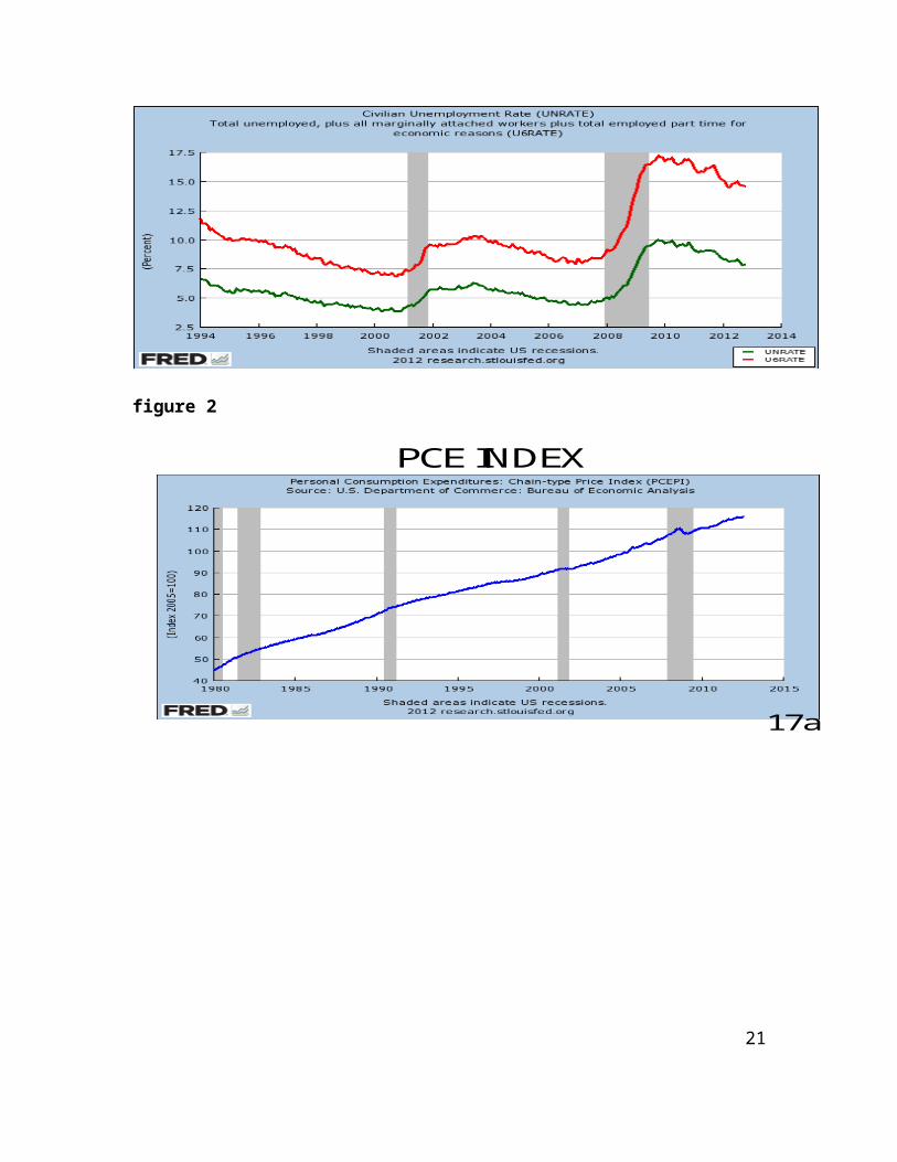
figure 2

PCE INDEX

17a

21

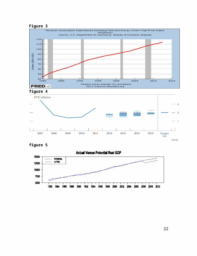
Figure 3

figure 4

figure 5

22

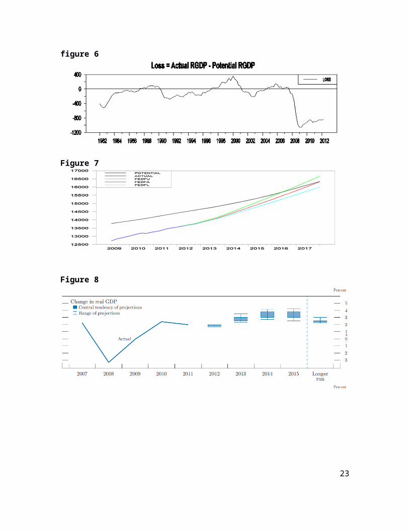
figure 6

Figure 7

Figure 8

23

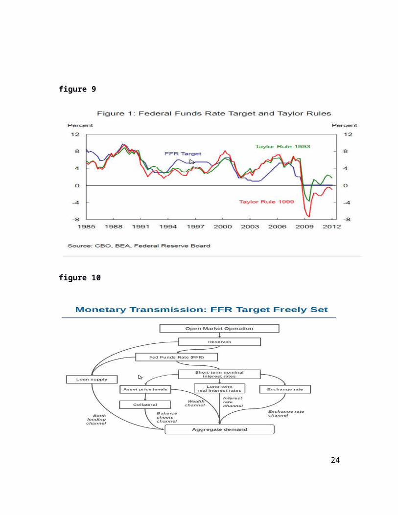
figure 9

figure 10

24

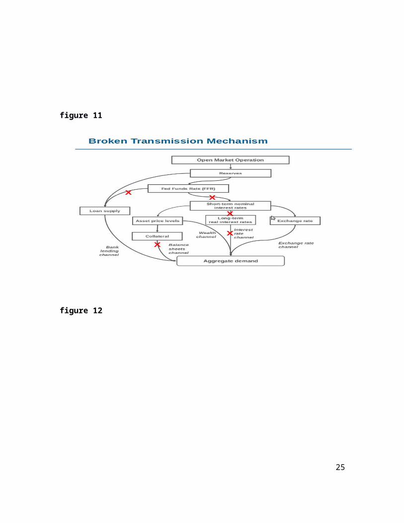
figure 11

figure 12

25

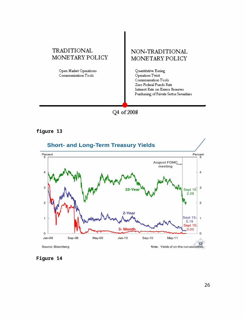
figure 13

Figure 14

26

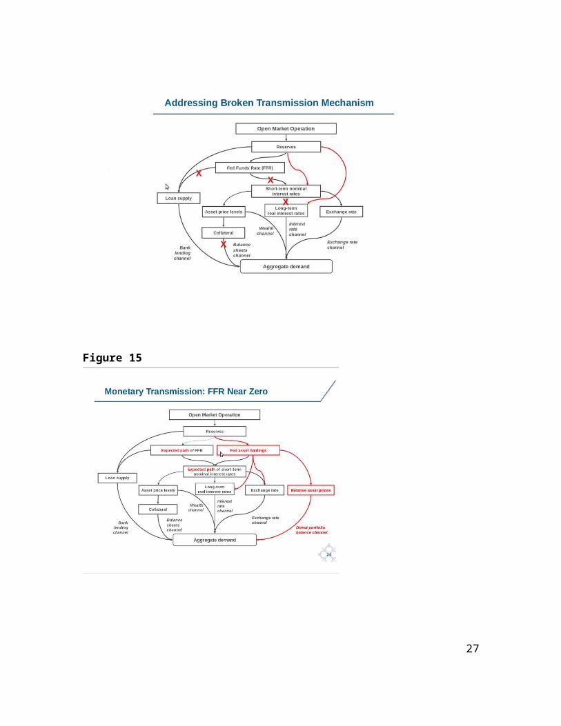
Figure 15

27

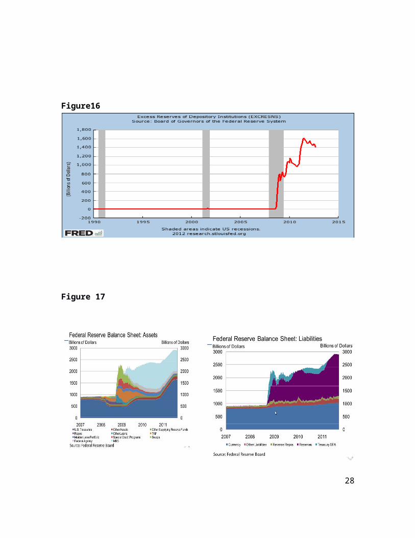
Figure16

Figure 17

28

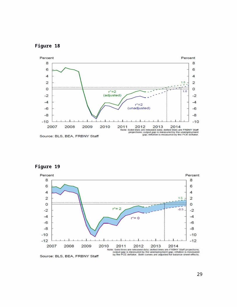
Figure 18

Figure 19

29