Embed Size (px)
Citation preview
Electronic copy available at: http://ssrn.com/abstract=1861229
Till Labor Cost Do Us Part A Vecm Model of Unit Labor Cost Convergence
in the Euro Area
Francesca Pancotto Filippo Pericoli
Quaderni - Working Paper DSE N° 759

Electronic copy available at: http://ssrn.com/abstract=1861229
Till Labor Cost Do Us Part
A Vecm Model of Unit Labor Cost Convergence in the
Euro Area*.
Francesca Pancotto�, and Filippo Pericoli�
June 6, 2011
Abstract
A sustainable path of relative competitiveness among the EMU countries is a
key factor for the survivorship of the currency union in the long run. We analyze
unit labor costs in the European Union with VECM methodology to evaluate relative
competitiveness of euro area countries, controlling for exchange rate on the adjustment
dynamics, for the economy as a whole and for the manufacturing sector, considered
as a proxy of the tradable sector. Results show a lack of convergence of member
countries, which is more pronounced for the tradable sector. Persisting idiosyncratic
dynamics may be driven by di�erent bargaining policies and institutional structures
of national labor markets, and by di�erential path of technological advance deterring
convergence of long run productivity.
JEL codes: E31, O47, C32. Keywords: Unit labor costs, Exchange Rates, Conver-
gence, Competitiveness, Manufacturing Sector.
*The usual disclaimer applies.�Department of Economics, University of Bologna Piazza Scaravilli 2, Bologna, Italy, Corresponding
author: [email protected]�Italy's Ministry of Finance, Via XX Settembre 97, Roma, Italy and CEIS Economics Foundation of
Tor Vergata University of Roma, Via Columbia 2, Roma, Italy
1

1 Introduction
Competitiveness in the euro area is a key issue for the survivorship of the Monetary Union.
Indeed, competitiveness is not only related to the growth of the single countries but also
to the economic cohesion of the union itself, given the very high level of interdependence
that the single currency has created among member countries. European countries are
characterized by an intrinsic diversity that in many ways is a richness and an opportunity:
nonetheless, it is fundamental that this diversity does not lead to large and persistent di-
vergences that can undermine the future of the union itself. To this purpose since 2007,
the European Central Bank has established rules for a systematic surveillance of member
states relative competitiveness, within their speci�c national settings, aimed at maintain-
ing a common framework that should help countries to identify imbalances and consolidate
relative competitiveness. Convergence is monitored by means of seven indicators of com-
petitive gaps: current account de�cits, unit labor costs, the stock of a country's net external
debt as a ratio to GDP, the national in�ation rate, the current account de�cit as a ratio to
GDP, the private and government debt ratios, the stock of private sector credit (European
Central Bank, 2011). Any sign of divergence of these indicators from the union average, is
a signal that should be taken into account when evaluating sustainability. Our choice is to
analyze unit labor costs (ULC), that measures the average cost of labor per unit of output:
it informs us on the relative dynamics of wages and productivity in the countries of the
union and on the relationship among them. It represents a direct link between productivity
and the cost of labor used in generating output. Unit labor cost dynamics corresponds to
the di�erence between compensation of employees and productivity: as important compo-
nent of in�ation dynamics, it may undermine relative competitiveness of a country. ULC is
moreover a relatively stable component of the price dynamics with respect to more volatile
determinants of price levels such as raw materials, commodity prices.
In the perspective of a monetary union, the relationship between labor costs among
member countries takes an even more important role as it expresses the degree of homo-
geneity, integration (and/or complementarity) of the member states. In a recent paper,
2

Dullien and Fritsche (2007) analyze unit labor cost trends in the euro area with the aim
to evaluate the degree of convergence of the member states in terms of both wage and
productivity trends. They �rst examine unit labor cost developments before and after the
introduction of the single currency and secondly compare the performance of the coun-
tries of the euro area with other currency unions, namely the regions of United States of
America and Länder of the Federal Republic of Germany. They implement a cointegration
approach on unit labor cost growth rates and test convergence with respect to the union
average. The analysis �nds evidence of cointegration and thus convergence of ULC but at
the same time the comparison with the performance of the other currency unions is not in
favor of Euro area, where deviations from area-wide averages are much larger than in the
US regions as well as in German Länders. Moreover, it is of their concern, the presence of
a tendency towards deviation in the last years of the sample, in particular for Germany.
In this work, we extend their contribution on ULC convergence in two directions. First,
we enlarge the data sample to observations up to 2010. Second, we inspect more deeply
the components of ULC in a VECM model of growth rates examining ULC in both trad-
able and non tradable sectors. Bertola (2008) shows some concern related to the ability
of ULC to provide information on the relative competitiveness of euro area members and
wage dynamics, in particular in the comparison between tradable and non tradable sector:
his concerns are basically twofold. First, the comparability of data among member coun-
tries is a�ected by a low degree of homogeneity of data collection mechanisms; secondly,
the Balassa-Samuelson e�ect can bias the information contained in the available data.
Notwithstanding these issues, we believe that an inspection of the behavior of ULC for the
total economy and manufacturing sector, could give important insights on the dynamics
of competitiveness of the currency union members.
A contribution similar to ours is the one of Tatierska (2008), which disaggregates ULC
in 4 sub-sectors and uses quarterly data up to the second quarter of 2007. Our work adds
to hers in the data sample considered and in the methodology used: while she assesses
cointegration mainly by means of an ? methodology applied to a single country of the area
and a panel Pedroni test (?), we investigate over the existence of a long run relationship
3

with the Joh (1988) approach, which we believe to be the most appropriate tool in a contest
of highly heterogeneous and interacting countries.
In this way we are able to answer the very fundamental research question of whether
a single country has a competitiveness level which is in equilibrium with that experienced
in the rest of the area as a whole. Moreover, within this framework we are able to test the
hypothesis of weak exogeneity which means verifying the hypothesis that a country ULC
does not a�ect the euro area, thus implying that its dynamics is not taken into account
from other euro area countries in the adjustment toward the equilibrium. Finally we are
able to test if the cointegrating vector has an economically desirable content, i.e. it is of
the type (1,-1): this hypothesis is equivalent to the two testable restrictions that the linear
trend is excludable from the cointegrating vector and that the considered country has a
stable relative competitiveness within the area. By taking into account tradable and non
tradable sector unit labor costs, we can shed some light on the reasons of the persistent
divergent dynamics of EMU labor costs.
The rest of the paper is organized as follows. In Section 2 we explore literature contri-
butions related and relevant for our work. In section 3 we describe the database used for
the analysis with some preliminary statistical analysis and present the empirical method-
ology implemented in the following section. In section 4 we report estimates results. In
section 5 we draw some conclusions and policy implications.
2 Literature Review
In a seminal paper, Baumol (1986) identi�es the mechanism that allows convergence in
industrialized economies as the result of spillover e�ects that innovation and investment in
a country generate in near-by countries: countries at a lower level of development absorb
part of the e�ects of innovation and increase their productivity, allowing income growth
and wage increases. Spillover e�ects would hold only if technology is supposed identical in
all the countries involved: countries with a lower technological advancement may not be
completely capable to take advantage of these spillover e�ects and consequently not being
4

able to catch up with the productivity advancements of the leader. The e�ects of this type
of misalignment could be observed in the dynamics of labor costs, a�ected by productivity,
by de�nition. If we hypothesize that tradable sector goods are more a�ected by innovation
spillovers than non-tradable sector, we should observe a di�erent behavior of the two labor
costs when analyzed separately. Convergence in the tradable sector should consequently
be more pronounced if the member countries are moving towards a similar technological
pattern.
The risk that euro area countries could be on diverging technological pattern would be
coherent in a framework with cumulative knowledge and increasing returns at the basis
of innovation and technological change (Dosi, 1988): countries characterized by a higher
initial technological development, and/or knowledge advancement, would be already in a
diverging path leading to a systematic better competitiveness performance, once the scope
for beggar-thy-neighbor policies are removed, as it is the case for the EMU.
Krugman (1991) points instead at pecuniary external economies as the source of possible
divergence among regions, in a core-periphery model characterized by increasing returns
in the manufacturing sector. Convergence or divergence is determined by the dynamics of
manufacturing labor force with respect to the wage rate. If the share of manufacturing
workers decreases with the increase of the relative wage of the central region, the dynamics
is convergent: workers migrate out of the region having a larger work force. If instead,
the share of manufacturing workers in central region increases with the wage rate, workers
will tend to migrate into the region that already has more workers, and this will cause
divergence. The wage rate would be steadily higher in the economy with larger market.
In the smaller region, to guarantee employment, a wage di�erential would be required in
order to allow employment, thus justifying a persistent diverging dynamics of wages in
peripheral countries.
ULC comparison between tradable and non-tradable can shed some light on the mecha-
nism in which price and unit labor cost increases in the non-tradable sector impact on unit
labor costs in the tradable sector. Tradable goods are subject to higher degree of interna-
tional competition and consequently adjust more strongly to shocks and �uctuations from
5

international markets. Non-tradable sectors instead, can bene�t from a more protected
price dynamics and consequently have guaranteed a higher average level of wages. Salido
et al. (2005) for example take into account this e�ect exploring determinants and macroe-
conomic implications of persistent in�ation di�erentials in Spain within EMU. They show
that larger demand of non-tradable goods and real-wage rigidities are crucial in explaining
diverging price developments in Spain. Unit labor costs in non-tradable sector a�ect the
productions costs of tradable goods and reduce the competitiveness of the tradable sector as
well. Relatedly, Zemanek et al. (2010) analyze intra-euro area current account persistently
divergent balances. In particular, they investigate how the impact of structural reforms
from the public and the private sector a�ect the current account balance. They argue that
current account divergences in the euro area may have been determined by in�ationary
pressures coming from the non-tradable sector: �rstly as non tradable goods are used as
inputs for tradable goods, thus in�uencing the price of tradable goods as well; secondly,
through an imitation e�ect of the wages of the non-tradable (where wages are more rigid)
from the wages of the tradable sector. They call it reversed Balassa-Samuelson e�ect, "...
where rising wages in the non-tradable sector trigger wage adjustment in the traded goods
sector, which might reduce the current account balance." Zemanek et al. (2010)
In a di�erent dimension, the comparison between tradable and non tradable unit labor
costs, are relevant in the discussion related to the impact of the development of public sector
wages on the convergence dynamics. Public sector wages account on average for more than
10% of GDP and more than 20% of the total compensation of employees. Clearly, public
wage increases constitute a strong signal for private sector wage negotiations: the larger
the public sector is, compared with the tradable sector, the stronger will be the signal
for wages in the private sector, and therefore the in�uence on the unit labor costs in the
private sector, taking into account also productivity. Hence, the larger the public sector,
the more important, and the more challenging, will be its role in the overall evolution of
cost competitiveness (Trichet, 2011). Evidence reveals an important in�uence from public
sector wages to private wages in many euro area countries. Public wage spillovers seem to
be particularly important in countries that have experienced high and volatile public wage
6
growth. Public sector wages may be responsible for rapid increases in unit labor costs and
misaligned intra-euro area competitiveness (Pérez and Sanchez, 2010; Lamo et al., 2008).
3 Data and Methodology
Data
For the purpose of our analysis we employ annual data for the following countries adhering
to the European Monetary Union: Austria, Belgium, Finland, France, Germany, Greece,
Ireland, Italy, Luxembourg, Netherlands, Portugal and Spain. We included in the dataset
all the eleven countries that entered the Union on January 1st 1999, plus Greece that joined
the union two years later, on January 1st 2001. This choice has been done with the aim
of considering a set of countries which are homogeneous as regards the duration of their
membership to the common currency area.
The empirical analysis has been performed at yearly frequency and historical series
have been obtained by the source AMECO, the on-line database provided by the Euro-
pean Commission. Our empirical analysis focuses on unit labor cost �gures for the whole
economy and for the manufacturing sector. With regards to the total economy, we built
unit labor cost �gures as compensation of employees1 divided by the gross national income
at constant prices2, while with regards to the manufacturing sector, unit labor cost �gures
have been obtained as the ratio of sectoral compensation of employee3 to sectoral value
added at constant prices4. Both variables, expressed in national currencies, have been
converted in ecu/euro units by employing the �gures for nominal bilateral exchange rate
of a given national currency versus ecu/euro (units of national currency per ecu/euro).5
The key point of the empirical analysis consists in the comparison of unit labor costs in
the i-th country of the euro area with unit labor costs �gures registered in the remaining
1Ameco database code: UWCD.2Ameco database code: OVGD.3Ameco database code: ISIC D UWCM.4Ameco database code: ISIC D OVGM.5Ameco database code: XNE.
7
countries. To this aim, for every country of the sample we have computed average unit labor
cost �gures in the remaining countries by removing from the calculation the i-th country
itself. Indeed, especially in the case of big countries such as Germany, France or Italy,
a comparison with euro area average (included the country itself) may produce a biased
picture of real underlying unit labor cost dynamics. The same calculation has been repeated
for each country of the euro area, for the total economy and for the manufacturing sector.
Lastly all variables included in the foregoing analysis have been expressed in logarithms
in order to attenuate heteroskedasticity and to allow a simple economic interpretation for
the estimated parameters.
Preliminary data analysis
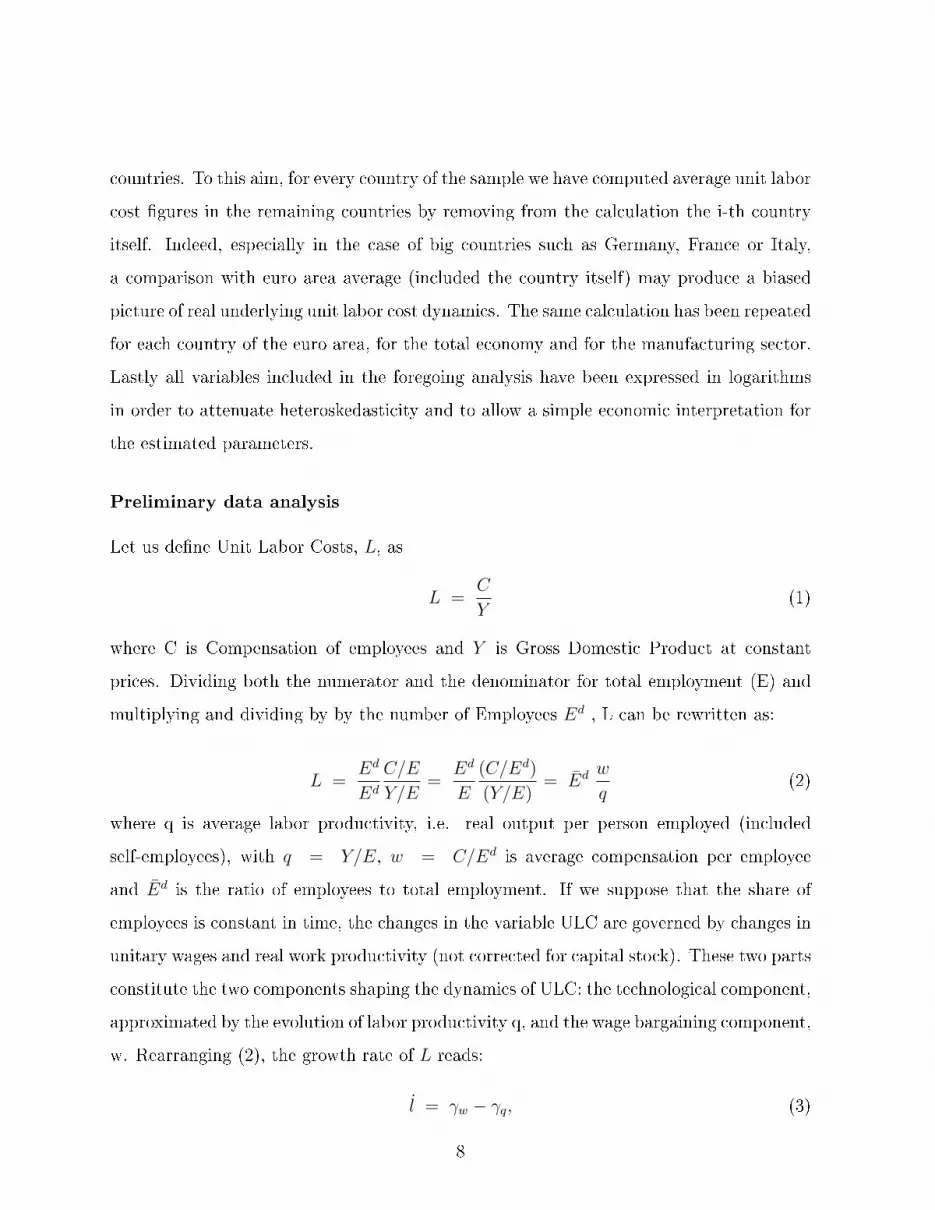
Let us de�ne Unit Labor Costs, L, as
L =C
Y(1)
where C is Compensation of employees and Y is Gross Domestic Product at constant
prices. Dividing both the numerator and the denominator for total employment (E) and
multiplying and dividing by by the number of Employees Ed , L can be rewritten as:
L =Ed
Ed
C/E
Y/E=
Ed
E
(C/Ed)
(Y/E)= Ed w
q(2)
where q is average labor productivity, i.e. real output per person employed (included
self-employees), with q = Y/E, w = C/Ed is average compensation per employee
and Ed is the ratio of employees to total employment. If we suppose that the share of
employees is constant in time, the changes in the variable ULC are governed by changes in
unitary wages and real work productivity (not corrected for capital stock). These two parts
constitute the two components shaping the dynamics of ULC: the technological component,
approximated by the evolution of labor productivity q, and the wage bargaining component,
w. Rearranging (2), the growth rate of L reads:
l = γw − γq, (3)
8

where γw = wwand γq = q
q. Consequently:
γq = γw − l (4)
which means that from the di�erence between γw and l we obtain a measure of the dynamics
of productivity. When productivity is growing at a positive rate, unit labor cost grows at
a rate lower than the one of wages.
With these simple identities at hand, we explore the evolution of ULC in the euro area
countries compared with the union average in Fig. 6.1. From the simple inspection of the
log levels of ULC, in black, we observe how di�erent is the behavior of the countries of
the union with respect to the union average, reported in gray. Austria, Belgium, France,
Luxembourg and Netherlands, show a pattern that is substantially in line with the euro
area, while a di�erent story can be told for the other countries. Finland, has a converging
pattern from 1995 on, while before that date, values were substantially over the mean.
Italy, Ireland and Greece show a level persistently below the euro area, while Spain and
Portugal, present a crossing line with the union average, from lower to higher than the
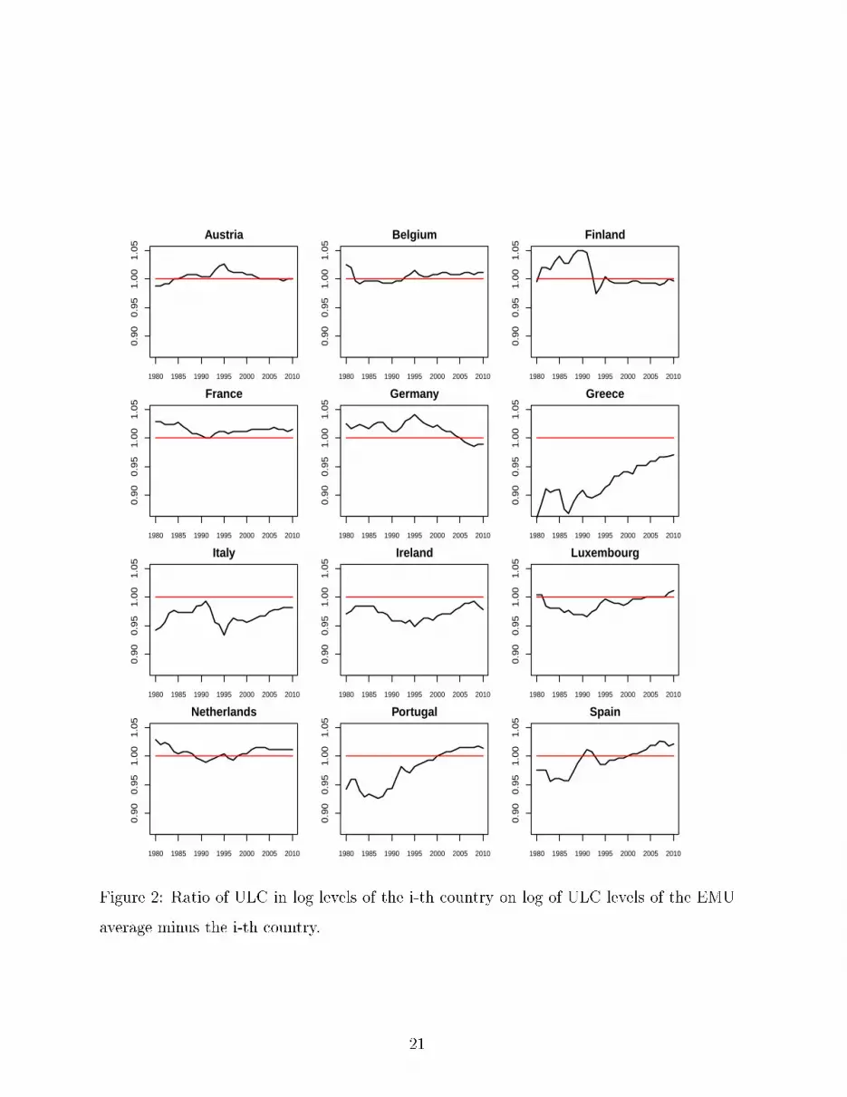
average pattern around year 2000. If we observe in the ratio of ULC in the i-th country
to ULC in the rest of the euro area (see �gure 6.1), we can have a more precise idea
of the dynamics of the variable with respect to the mean: northern countries show a
substantial stability around the euro average, while the same cannot be told for the others.
In particular the increasing trend of Portugal and Spain in the last years is quite evident,
as well as for Greece but for a level well below the average of the union. Ireland and Italy
are substantially below the average while a completely di�erent picture is now clearer for
Germany: with the creation of the currency union, the country has managed to obtain a
substantial and systematic reduction of ULC, with a diverging pattern relatively to all the
other countries.
With regards to the manufacturing sector (see �gure 6.1), �gures are slightly di�er-
ent from those relative to the total economy previously observed. Austria, Belgium and
Netherlands, keep a level of ULC in line with the area trend, while some di�erence is
9

observed for Luxembourg, with a spike in ULC for manufacturing sector after the begin-
ning of the currency union. Portugal and Spain on the other hand, show a growing trend
in a dynamics of catching up with the union average, with a �nal overcome in 2005 for
Spain and 2007 for Portugal. The same catching up can be identi�ed for Italy and Greece,
despite the latter begins with a lower value. It is important to notice how Germany has
improved its relative competitive position with the participation to the common currency
area, France ha not registered substantial changes, while Italy, Greece, Portugal and Spain
have su�ered a signi�cant worsening in their competitiveness dynamics with respect to
tendencies observed before the institution of the common currency. From �gure 6.1 we can
also identify the peculiar cases of Ireland and Finland that during the timespan considered
have experienced a negative trend in unit labor cost in the manufacturing sector. To sum
up, a simple inspection of the time series of Unit labor costs reveals that southern countries
are on a diverging path and that, on the opposite side, Germany is also strongly diverging
from the rest of the area. Our results would con�rm the analysis of Verspagen (2010) on
patterns of technological and economic growth suggesting the presence of a dividing line
between the southwest and northeast of Europe6.
Methodology
We investigate over the existence and the shape of long run stable economic relationships
within the multivariate approach to cointegration provided by Joh (1988) and Johansen
and Juselius (1990). The main advantage of this approach is that it provides a likelihood-
ratio based test that can be applied to determine the cointegration rank which character-
izes any arbitrary set of endogenous variables. It is a well known fact that the performance
of this test in terms of size and power may be not optimal in small samples, given that
the asymptotic distributions are generally poor approximations to the true distributions
(Juselius, 2006). In the following we apply the aforementioned methodology to a sample of
31 observations for the economy as a whole (years 1980-2010) and for the manufacturing
6It is noteworthy however that in this contribution the author considers a larger group of countries.
10

sector (years 1979-2009). Even if this is not a large sample in terms of number of observa-
tions, there is a number of facts which make our analysis robust to small sample biases. ?
have proven that when investigating over long run relationship the timespan considered is
more relevant than the frequency of observations, which means that a sample of N yearly
observations is more informative than a sample of N quarterly observations. The validity
of this �nding has been extended by Hu (2008), who shows, within the Johansen's frame-
work by means of Monte Carlo simulations, that the performance of the test is better the
longer the timespan considered. Moreover, Gonzalo and Pitarakis (1999) have shown that
for a given sample size the performance of the cointegration test is better the lower the
dimensionality of the system which in our case is only two. Last, we have veri�ed that the
results of the tests on the cointegration rank and the results of the tests on the restrictions
on the cointegrating vectors remain valid7 even if we take into account the small sample
Bartlett correction proposed by ?.
In order to investigate the existence of a stable relation between the Euro area (excluded
the i-th country) unit labor cost and the single i-th country dynamics, we test the presence
of a cointegration relationship between these two elements. From an econometric point of
view, we consider a bi-dimensional VAR model:
Xt = φ+ A1Xt−1 + ...AkXt−k + εt (5)
where Xt is a (2x1) vector containing the two series for unit labor costs in ecu/euro for the
i-th country and for the rest of the area, i.e. Xt = [lt, leut], Ai is the generic (2x2) matrix
of parameters with i = (1, ..., k); φ is a vector of constants; εt is the error component of the
model that is assumed to follow a multinormal distribution. Juselius (2006) shows that if
the variables included in the system are integrated of order one, the preceding model can
be re-parametrized as:
∆Xt = α(β′Xt−1) + µ0 + µ1t+ Γ1∆Xt−1 + ...Γk−1Xt−k+1 + εt (6)
7Results unreported but available on request.
11

where the product β′Xt−k is a vector of stationary cointegration relations which describe
the long run behavior of the system, which are at most (n−1). The number of cointegrating
relationships can be determined by investigating over the rank of the matrix Π = αβ′, by
means of the likelihood ratio-based maximum eigenvalue (λ-max) and trace tests.
In general it is not known whether there are linear trends in some of the variables, or
whether they cancel in the cointegrating relations or not. Five di�erent models are possible
arising from the imposition of di�erent restrictions on the deterministic components in
Eq. (6). From the inspection of time series we can clearly exclude from the analysis
those models which assume no linear trend in the data (two out of �ve models proposed
by Juselius (2006)). Moreover we can also exclude a model with a linear trend in the
di�erenced variables, i.e. with a quadratic trend in data. Thus there remain two types of
model available for the analysis. In the �rst type of model (model 1 thereafter) we include
a constant in the VAR model in di�erences, a formulation which allows for a linear trend in
data but we do not include a trend in the cointegrating space. The other model available
(model 2 thereafter) includes not only a constant in the VAR model in di�erences and thus
a linear trend in data, but also a linear trend in the cointegrating space which is restricted
to cancel out in the �rst-di�erenced parametrization of the model. As regards the lag
length determination of the VAR model, we have chosen to follow the results arising from
the Schwartz Information Criterium which almost always indicates an optimal lag of one
for the VAR model in the levels of variables, which corresponds to an optimal lag of order
zero for the model as expressed in the VECM reparametrization. Only in a few cases, in
order to �nd cointegration, we have allowed for a lag length of two for the VAR in level
which corresponds to a lag length of one for the VECM version of the model. Given the
aforementioned choices, in our case the VECM model as from Eq. (6), becomes :
∆Xt = α(β′Xt−k) + µ0 + Γ1∆Xt−1 + εt (7)
It is important to notice that cointegration analysis can be interpreted as a convergence
test with some limitations: �rst, a country being on a catch up path might lack cointegra-
12
tion property with respect to the union average but being nonetheless on a fruitful pattern.
Secondly, cointegration tests are sensitive to the particular sample considered: in our case
we decided to employ the timespan 1980-2010 for the total economy (years 1979-2009 for
the manufacturing sector) because we believe that this is a period characterized by a rel-
atively stable macroeconomic environment, and at the same time it consists of a minimal
number of observations, at annual frequency and in a bidimensional system, for applying
the Johansen's methodology and estimating the cointegrating vectors.
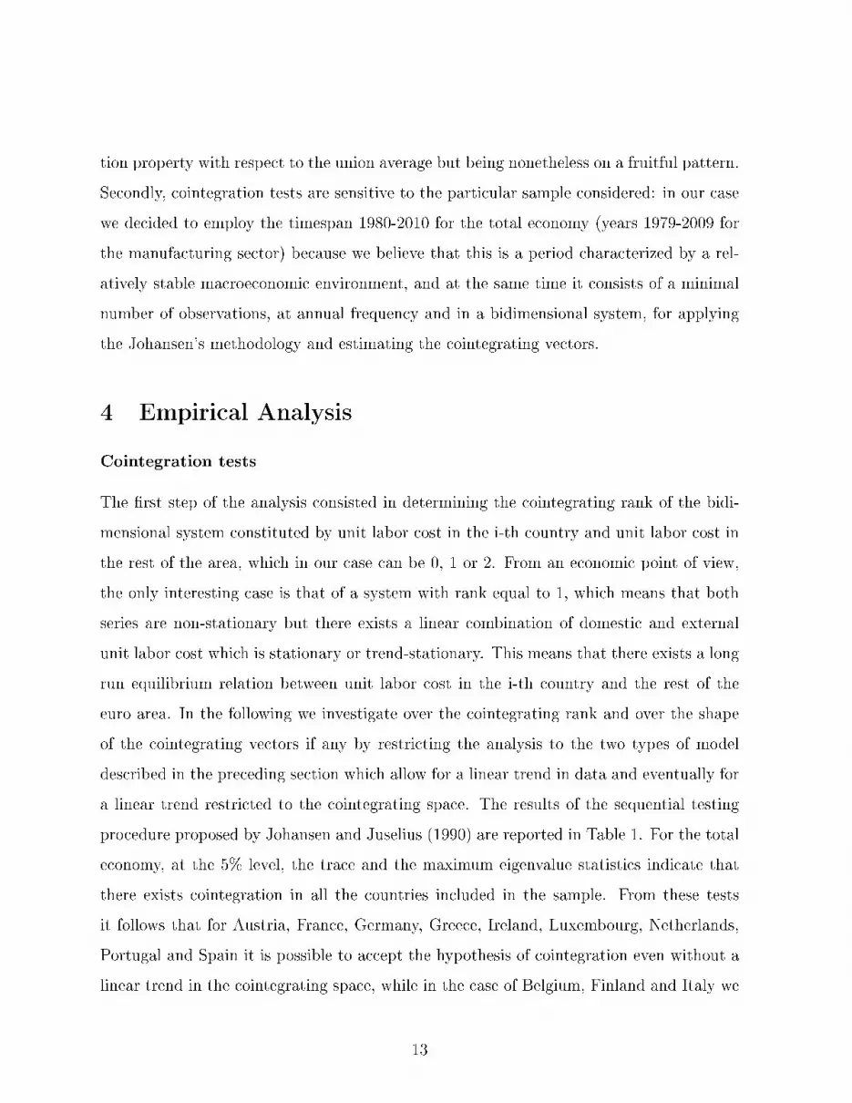
4 Empirical Analysis
Cointegration tests
The �rst step of the analysis consisted in determining the cointegrating rank of the bidi-
mensional system constituted by unit labor cost in the i-th country and unit labor cost in
the rest of the area, which in our case can be 0, 1 or 2. From an economic point of view,
the only interesting case is that of a system with rank equal to 1, which means that both
series are non-stationary but there exists a linear combination of domestic and external
unit labor cost which is stationary or trend-stationary. This means that there exists a long
run equilibrium relation between unit labor cost in the i-th country and the rest of the
euro area. In the following we investigate over the cointegrating rank and over the shape
of the cointegrating vectors if any by restricting the analysis to the two types of model
described in the preceding section which allow for a linear trend in data and eventually for
a linear trend restricted to the cointegrating space. The results of the sequential testing
procedure proposed by Johansen and Juselius (1990) are reported in Table 1. For the total
economy, at the 5% level, the trace and the maximum eigenvalue statistics indicate that
there exists cointegration in all the countries included in the sample. From these tests
it follows that for Austria, France, Germany, Greece, Ireland, Luxembourg, Netherlands,
Portugal and Spain it is possible to accept the hypothesis of cointegration even without a
linear trend in the cointegrating space, while in the case of Belgium, Finland and Italy we
13

obtain that it is necessary to include a linear trend in the long run behavior of the system in
order to achieve cointegration. On the whole these tests show that there exists a long run
statistical equilibrium between each country of the euro area and the rest of the area, but
this cannot considered as an empirical evidence of euro area sustainability for the shape of
the cointegrating space may produce unsustainable economic consequences. With regards
to the manufacturing sector the results of the tests are less favorable. Indeed, apart from
the case of Luxembourg for which there are not enough observations to make the test, we
accept the hypothesis of cointegration in nine out of eleven countries (Austria, Finland,
Germany, Greece, Ireland, Italy, Netherland, Portugal and Spain), while in the case of
Belgium and France we reject the hypothesis of cointegration. From the results of the tests
it follows that we can accept the hypothesis of cointegration without a linear trend in the
cases of Austria, Finland, Greece, Ireland, Italy and Spain, while in the cases of Germany,
Netherlands and Portugal it is necessary to include a linear trend in the cointegrating space
in order to achieve cointegration.
Cointegrating vectors
Table 3 reports the cointegrating vectors obtained from the reduced rank estimate of the
VECM models normalized on the unit labor cost in the i-th country. As regards the
estimates conducted for the total economy, it results that in all cases the coe�cients have
the right "negative" sign. This means that in the long run there exists a positive log-
linear function which links unit labor cost in the i-th country and unit labor cost in the
rest of the countries considered as a whole. Notwithstanding, the analysis reveals the
existence of remarkable di�erences among countries in the long run. Indeed, Germany
and Austria are characterized by a stable tendency toward a relative decrease of unit
labor costs while the rest of the countries considered are characterized by an opposite
tendency. The parameters of Belgium, Finland and Italy are not directly comparable
in terms of relative competitiveness due to the presence in the cointegrating space of a
linear trend. The results are di�erent in the case we consider relative unit labor cost
14

dynamics in the manufacturing sector alone. In this case we �nd that Finland and Ireland
are characterized by a cointegrating vectors with the wrong "positive" sign which means
that the higher unit labor cost in other countries, the lower in these two countries that
is a synthetic transposition of the results evident from �gure 3. Moreover, it is con�rmed
the �nding that Germany and Austria exhibit a stable tendency toward increasing their
relative competitiveness. The path of Germany results even more divergent given the
presence in the cointegrating space of a negative trend which sums to the e�ect arising
from an elasticity less than unity.
Weak exogeneity tests
After having estimated the VECM models for the total economy and for the manufactur-
ing sector, we proceeded to test some economically relevant hypothesis starting from the
unrestricted versions of the models. First we have conducted a test of weak exogeneity for
unit labor cost in the generic i-th country. This test is done by verifying the likelihood
of the assumption that in the VECM model the loading factor of disequilibrium in the
i-th country is equal to zero in the equation for unit labor cost dynamics in the rest of
countries as a whole. From the results of these tests, reported on table 4, it follows that
the hypothesis of weak exogeneity is always rejected by data for the total economy as well
as for the manufacturing sector alone. This result may seem counterintuitive in a normal
setting given that one generally expects that a small country such as Ireland or Belgium
should not a�ect unit labor cost dynamics in a big country such as Germany. However we
remark that our model is deliberately not structural as our goal consists in examining long
run tendencies in unit labor cost dynamics rather than understanding real data generating
processes. This means that the rejection of the hypothesis of weak exogeneity should not
be regarded as an evidence of the economic importance of a given country. Rather we be-
lieve that there may exist common factors which drive unit labor cost dynamics in small as
well as in big countries and that these factors render endogenous unit labor cost dynamics
in small countries.
15

Relative convergence tests
Lastly we have tested the hypothesis that the β vector has the particular form (1,-1),
which means that the elasticity of unit labor cost in the generic i-th country with respect
to unit labor cost in the rest of countries as a whole is unitary. From an economic point
of view this means that the relative competitiveness of a given country is constant in the
long run and this test notwithstanding some limitations can be assimilated to a test of
economic sustainability of the currency union. From the results of the test reported on
table 5 it emerges that the hypothesis of relative convergence is always strongly rejected
by data. This means that even if we did �nd a stable statistical relation, the shape of the
cointegrating vector is such that euro area countries exhibit tendency to diverge in terms
of relative competitiveness. These diverging dynamics may produce unsustainable e�ects
on intra-area trade balances and resource allocations given that unit labor costs represent
the most important factor in the determination of producer prices.
5 Concluding remarks
The analysis performed underlines that euro area countries are characterized by diverging
tendencies in unit labor cost dynamics which result in persistent gain or losses of compet-
itiveness with respect to the rest of countries of the area as a whole. A simple inspection
of data reveals that after the introduction of the euro, divergences in relative competitive
positions have increased and our econometric analysis �nds that this is a persistent, not
mean-reverting process. This �nding is true not only for the economy as a whole but also
for the manufacturing sector, which produces the overwhelming majority of traded goods.
Given the high degree of international competition currently reached we believe that these
divergences are not sustainable and may result in a progressive reduction of the role played
by the manufacturing sector in those countries which experience a relatively sustained trend
in unit labor cost dynamics. Our econometric analysis support this evidence by �nding
that relative competitiveness is not stable and this process is not mean-reverting. In our
16

analysis we limit ourselves to the observation unit labor cost dynamics without distinguish-
ing between the role played wage bargaining policies and that of technological progress,
i.e. by productivity gains. The identi�cation of the separate role of these two factor in
driving national unit labor cost dynamics remains an issue open for future research.
17
References
(1988). Statistical analysis of cointegration vectors. Journal of Economic Dynamics and
Control 12 (2-3), 231 � 254.
Baumol, W. J. (1986). Productivity growth, convergence, and welfare: What the long-run
data show. The American Economic Review 76 (5), 1072�1085.
Bertola, G. (2008). Labor markets in emu: What has changed and what needs to change.
Economic Papers European Economy (338).
Dosi, G. (1988). Sources, procedures, and microeconomic e�ects of innovation. Journal of
Economic Literature 26 (3), pp. 1120�1171.
Dullien, S. and U. Fritsche (2007, March). Does the dispersion of unit labor cost dynamics
in the emu imply long-run divergence? results from a comparison with the united states
of america and germany. DIW Discussion Paper (674), 1 � 37.
Gonzalo, J. and J. Pitarakis (1999). Cointegration, Causality and Forecasting: A Festschrift
in Honour of C. W. J. Granger. Robert E. Engle and Halbert White.
Hu, W. (2008). Time aggregation and skip sampling in cointegration tests. Statistical
Papers 3, 116 � 133.
Johansen, S. and K. Juselius (1990). Maximum likelihood estimation and inference on coin-
tegration � with applications to the demand for money. Oxford Bulletin of Economics
and Statistics 52 (2), 169�210.
Juselius, K. (2006). The Cointegrated Var Model, Chapter 6. Advanced Texts in Econo-
metrics, Oxford University Press: Oxford.
Krugman, P. (1991). Increasing returns and economic geography. The Journal of Political
Economy 99 (3), pp. 483�499.
18

Lamo, A., J. J. Pérez, and L. Schuknecht (2008). Public and private sector wages: co-
movement and causality. ECB Working Paper 963.
Pérez, J. J. and A. J. Sanchez (2010, 1). Is there a signalling role for public wages? evidence
for the euro area based on macro data. ECB Working Paper 1148.
Salido, J. D. L., F. Restoy, and J. Vallés (2005, 3). In�ation di�erentials in emu: The
spanish case. Documentos de Trabajo.
Tatierska, S. (2008). Ulc dynamics of euro area countries and sr in the long run. Associa-
tionNational Bank of Slovakia WP 6.
Trichet, J. C. (2011, 2). Competitiveness and the smooth functioning of emu. European
Central Bank Speech, 23 February 2011 .
Verspagen, B. (2010). The spatial hierarchy of technological change and economic devel-
opment in europe. The Annals of Regional Science 45, 109�132.
Zemanek, H., A. Belke, and G. Schnabl (2010). Current account balances and structural
adjustment in the euro area. International Economics and Economic Policy 7, 83�127.
19

6 Appendix
6.1 Graphs and Tables
2.0
2.2
2.4
2.6
2.8
Austria
1980 1985 1990 1995 2000 2005 2010
2.0
2.2
2.4
2.6
2.8
Belgium
1980 1985 1990 1995 2000 2005 2010
2.0
2.2
2.4
2.6
2.8
Finland
1980 1985 1990 1995 2000 2005 2010
2.0
2.2
2.4
2.6
2.8
France
1980 1985 1990 1995 2000 2005 2010
2.0
2.2
2.4
2.6
2.8
Germany
1980 1985 1990 1995 2000 2005 2010
2.0
2.2
2.4
2.6
2.8
Greece
1980 1985 1990 1995 2000 2005 2010
2.0
2.2
2.4
2.6
2.8
Italy
1980 1985 1990 1995 2000 2005 2010
2.0
2.2
2.4
2.6
2.8
Ireland
1980 1985 1990 1995 2000 2005 2010
2.0
2.2
2.4
2.6
2.8
Luxembourg
1980 1985 1990 1995 2000 2005 2010
2.0
2.2
2.4
2.6
2.8
Netherlands
1980 1985 1990 1995 2000 2005 2010
2.0
2.2
2.4
2.6
2.8
Portugal
1980 1985 1990 1995 2000 2005 2010
2.0
2.2
2.4
2.6
2.8
Spain
1980 1985 1990 1995 2000 2005 2010
Figure 1: ULC in log levels of the i-th country in black; in grey log of ULC levels of the
EMU average minus the i-th country.
20
0.9
00
.95
1.0
01
.05
Austria
1980 1985 1990 1995 2000 2005 2010
0.9
00
.95
1.0
01
.05
Belgium
1980 1985 1990 1995 2000 2005 2010
0.9
00
.95
1.0
01
.05
Finland
1980 1985 1990 1995 2000 2005 2010
0.9
00
.95
1.0
01
.05
France
1980 1985 1990 1995 2000 2005 2010
0.9
00
.95
1.0
01
.05
Germany
1980 1985 1990 1995 2000 2005 2010
0.9
00
.95
1.0
01
.05
Greece
1980 1985 1990 1995 2000 2005 2010
0.9
00
.95
1.0
01
.05
Italy
1980 1985 1990 1995 2000 2005 2010
0.9
00
.95
1.0
01
.05
Ireland
1980 1985 1990 1995 2000 2005 2010
0.9
00
.95
1.0
01
.05
Luxembourg
1980 1985 1990 1995 2000 2005 2010
0.9
00
.95
1.0
01
.05
Netherlands
1980 1985 1990 1995 2000 2005 2010
0.9
00
.95
1.0
01
.05
Portugal
1980 1985 1990 1995 2000 2005 2010
0.9
00
.95
1.0
01
.05
Spain
1980 1985 1990 1995 2000 2005 2010
Figure 2: Ratio of ULC in log levels of the i-th country on log of ULC levels of the EMU
average minus the i-th country.
21

2.4
2.6
2.8
3.0
Austria
1980 1985 1990 1995 2000 2005
2.4
2.6
2.8
3.0
Belgium
1980 1985 1990 1995 2000 2005
2.4
2.6
2.8
3.0
Finland
1980 1985 1990 1995 2000 2005
2.4
2.6
2.8
3.0
France
1980 1985 1990 1995 2000 2005
2.4
2.6
2.8
3.0
Germany
1980 1985 1990 1995 2000 2005
2.4
2.6
2.8
3.0
Greece
1980 1985 1990 1995 2000 2005
2.4
2.6
2.8
3.0
Italy
1980 1985 1990 1995 2000 2005
2.4
2.6
2.8
3.0
Ireland
1980 1985 1990 1995 2000 2005
2.4
2.6
2.8
3.0
Luxembourg
1980 1985 1990 1995 2000 2005
2.4
2.6
2.8
3.0
Netherlands
1980 1985 1990 1995 2000 2005
2.4
2.6
2.8
3.0
Portugal
1980 1985 1990 1995 2000 2005
2.4
2.6
2.8
3.0
Spain
1980 1985 1990 1995 2000 2005
Figure 3: ULC of the manufacturing sector in log levels of the i-th country in black; in
grey log of ULC levels of the EMU average minus the i-th country.
22

0.9
00
.95
1.0
01
.05
Austria
1980 1985 1990 1995 2000 2005
0.9
00
.95
1.0
01
.05
Belgium
1980 1985 1990 1995 2000 2005
0.9
00
.95
1.0
01
.05
Finland
1980 1985 1990 1995 2000 2005
0.9
00
.95
1.0
01
.05
France
1980 1985 1990 1995 2000 2005
0.9
00
.95
1.0
01
.05
Germany
1980 1985 1990 1995 2000 2005
0.9
00
.95
1.0
01
.05
Greece
1980 1985 1990 1995 2000 2005
0.9
00
.95
1.0
01
.05
Italy
1980 1985 1990 1995 2000 2005
0.8
50
.95
1.0
5
Ireland
1980 1985 1990 1995 2000 2005
0.9
00
.95
1.0
01
.05
Luxembourg
1980 1985 1990 1995 2000 2005
0.9
00
.95
1.0
01
.05
Netherlands
1980 1985 1990 1995 2000 2005
0.9
00
.95
1.0
01
.05
Portugal
1980 1985 1990 1995 2000 2005
0.9
00
.95
1.0
01
.05
Spain
1980 1985 1990 1995 2000 2005
Figure 4: Ratio of ULC in log levels of the i-th country on log of ULC levels of the EMU
average minus the i-th country. Manufacturing Sector.
23

−0
.10
0.0
00
.10
0.2
0
Austria
1980 1985 1990 1995 2000 2005 2010
−0
.10
0.0
00
.10
0.2
0
Belgium
1980 1985 1990 1995 2000 2005 2010
−0
.10
0.0
00
.10
0.2
0
Finland
1980 1985 1990 1995 2000 2005 2010
−0
.10
0.0
00
.10
0.2
0
France
1980 1985 1990 1995 2000 2005 2010
−0
.10
0.0
00
.10
0.2
0
Germany
1980 1985 1990 1995 2000 2005 2010
−0
.10
0.0
00
.10
0.2
0
Greece
1980 1985 1990 1995 2000 2005 2010
−0
.10
0.0
00
.10
0.2
0
Italy
1980 1985 1990 1995 2000 2005 2010
−0
.10
0.0
00
.10
0.2
0
Ireland
1980 1985 1990 1995 2000 2005 2010
−0
.10
0.0
00
.10
0.2
0
Luxembourg
1980 1985 1990 1995 2000 2005 2010
−0
.10
0.0
00
.10
0.2
0
Netherlands
1980 1985 1990 1995 2000 2005 2010
−0
.10
0.0
00
.10
0.2
0
Portugal
1980 1985 1990 1995 2000 2005 2010
−0
.10
0.0
00
.10
0.2
0
Spain
1980 1985 1990 1995 2000 2005 2010
Figure 5: ULC growth in black and compensation per employee growth in red. Total
Economy
24

−0
.10
0.0
00
.10
0.2
0
Austria
1980 1985 1990 1995 2000 2005
−0
.10
0.0
00
.10
0.2
0
Belgium
1980 1985 1990 1995 2000 2005
−0
.10
0.0
00
.10
0.2
0
Finland
1980 1985 1990 1995 2000 2005
−0
.10
0.0
00
.10
0.2
0
France
1980 1985 1990 1995 2000 2005
−0
.10
0.0
00
.10
0.2
0
Germany
1980 1985 1990 1995 2000 2005
−0
.10
0.0
00
.10
0.2
0
Greece
1980 1985 1990 1995 2000 2005
−0
.10
0.0
00
.10
0.2
0
Italy
1980 1985 1990 1995 2000 2005
−0
.10
0.0
00
.10
0.2
0
Ireland
1980 1985 1990 1995 2000 2005
−0
.10
0.0
00
.10
0.2
0
Luxembourg
1980 1985 1990 1995 2000 2005
−0
.10
0.0
00
.10
0.2
0
Netherlands
1980 1985 1990 1995 2000 2005
−0
.10
0.0
00
.10
0.2
0
Portugal
1980 1985 1990 1995 2000 2005
−0
.10
0.0
00
.10
0.2
0
Spain
1980 1985 1990 1995 2000 2005
Figure 6: ULC growth in black and compensation per employee growth in red. Manufac-
turing Sector.
25

Table1:
Johansen-JuseliusCointegrationTest.
ULCGeneral
Econom
y.
Trace
λ-m
ax
Model1
Model2
Model1
Model2
H0:r=
0H
0:r≤
1H
0:r=
0H
0:r≤
1H
0:r=
0H
0:r≤
1H
0:r=
0H
0:r≤
1
H1:r=
1H
1:r=
2H
1:r=
1H
1:r=
2H
1:r=
1H
1:r=
2H
1:r=
1H
1:r=
2
Austria
38.85***
0.46
24.18**
10.52
38.39***
0.46
13.65
10.52
Belgium
40.80***
5.09**
45.55***
6.18
35.71***
5.09**
39.36***
6.18
Finland
37.21***
7.83***
53.17***
7.84
29.38***
7.83***
45.33***
7.84
France
28.99***
2.22
52.48***
8.42
26.76***
2.22
44.06***
8.42
Germany
38.26***
0.10
52.56***
14.35**
38.16***
0.10
38.21***
14.35**
Greece
31.88***
2.05
41.62***
7.87
29.82***
2.05
33.75***
7.87
Ireland
32.63***
3.79*
54.84***
12.04*
28.84***
3.79*
42.81***
12.04*
Italy
33.53***
5.17**
44.60***
7.35
28.36***
5.17**
37.25***
7.35
Luxem
bourg
33.79***
0.96
43.90***
4.80
32.84***
0.96
39.10***
4.80
Netherlands
35.02***
1.87
48.40***
7.61
33.15***
1.87
40.79***
7.61
Portugal
33.18***
1.53
38.20***
4.21
31.64***
1.53
33.99***
4.21
Spain
52.93***
1.67
54.27***
2.94
51.26***
1.67
51.33***
2.94
Notes:*,**,***,denote
statisticalsigni�cance
atthe10%,5%,1%
levels,respectively.
26
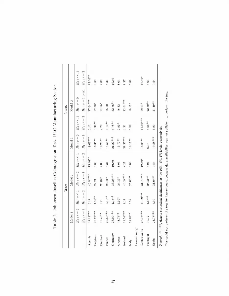
Table2:
Johansen-JuseliusCointegrationTest.
ULCManufacturingSector.
Trace
λ-m
ax
Model1
Model2
Model1
Model2
H0:r=
0H
0:r≤
1H
0:r=
0H
0:r≤
1H
0:r=
0H
0:r≤
1H
0:r=
0H
0:r≤
1
H1:r=
1H
1:r=
2H
1:r=
1H
1:r=
2H
1:r=
1H
1:r=
2H
1:r=
1p-val
H1:r=
2
Austria
19.19***
0.12
40.84***
13.20**
19.07***
0.12
27.64***
13.20**
Belgium
20.73***
4.38**
22.21
4.83
16.35**
4.38**
17.38*
4.83
Finland
18.48**
2.20
25.04*
7.08
16.28**
2.20
17.95*
7.08
France
20.66***
6.10**
23.41*
8.31
14.56**
6.10**
15.10
8.31
Germany
26.00***
4.78**
33.26***
10.50
21.22***
4.78**
22.76**
10.50
Greece
18.71**
2.99*
24.33*
8,01
15.72**
2.99*
16.32
8,01
Ireland
33.59***
2.21
40.28***
8.27
31.37***
2.21
32.01***
8.27
Italy
18.69**
0.58
25.00**
6.89
18.11**
0.58
18.11*
6.89
Luxem
bourg
°
Netherlands
27.73***
11.69***
31.70***
12.49*
16.04**
11.69***
19.21*
12.49*
Portugal
10.72
4.66**
28.31**
6.01
6.07
4.66**
22.30**
6.01
Spain
21.78***
1.90
31.03**
9.54
19.88***
1.90
21.49**
9.54
Notes:*,**,***,denote
statisticalsigni�cance
atthe10%,5%,1%
levels,respectively.
°Wecould
notperform
thetest
forLuxem
bourg
because
data
availabilitywasnotsu�cientto
perform
thetest.
27

Table 3: Cointegrating Vectors: Total Economy and Manufacturing Sector.
Total Economy
Ulc UlcEU Constant Trend
Austria 1 -0.65*** [-11.24] -0.92 - -
Belgium 1 -4.52*** [-6.01] 8.47 0.02*** [-6.00]
Finland 1 -6.09*** [-8.49] 11.91 0.04*** [5.09]
France 1 -2.34*** [-7.38] 3.49 - -
Germany 1 -0.33*** [-5.04] -1.79 - -
Greece 1 -3.65*** [-11.43] 7.20 - -
Ireland 1 -2.32*** [-9.38] 3.56 - -
Italy 1 -14.70*** [-5.73] 33.05 0.09*** [3.28]
Luxembourg 1 -1.70*** [-19.51] 1.86 - -
Netherlands 1 -1.82*** [-12.53] 2.14 - -
Portugal 1 -2.58*** [-18.33] 4.23 - -
Espain 1 -2.01*** [-20.69] 2.68 - -
Manufacturing Sector
Ulc UlcEU Constant Trend
Austria 1 -0.33*** [-3.39] -1.85 - -
Belgium - No cointegration - -
Finland 1 4.25*** [4.19] -14.44 - -
France - No cointegration
Germany 1 -0.50*** [-2.36] -1.88 0.00** [2.29]
Greece 1 -3.91** [-5.62] 8.12 - -
Ireland 1 2.72*** [8.54] -10.01 - -
Italy 1 -2.24*** [-7.31] 3.47 - -
Luxembourg - No data available - -
Netherlands 1 -0.25** [-2.17] -1.97 0.00** [-2.15]
Portugal 1 -0.35*** [-2.94] 1.43 -0.01*** [-7.67]
Espain 1 -2.42*** [-1.77] 3.95 - -
Note: *, **, ***, denote statistical signi�cance at the 10%,
5%, 1% levels, respectively. T-stats in brackets.
28

Table 4: Weak Exogeneity Test: Total Economy and Manufacturing Sector.
Total Economy
χ21 p-value
Austria 33.25 0.00
Belgium 24.11 0.00
Finland 32.91 0.00
France 14.56 0.00
Germany 24.31 0.00
Greece 28.34 0.00
Ireland 23.36 0.00
Italy 23.07 0.00
Luxembourg 9.77 0.00
Netherlands 23.77 0.00
Portugal 13.16 0.00
Espain 45.93 0.00
Manufacturing Sector
χ21 p-value
Austria 19.37 0.00
Belgium - No cointegration
Finland 9.74 0.00
France - No cointegration
Germany 19.64 0.00
Greece 11.64 0.00
Ireland 9.92 0.00
Italy 16.00 0.00
Luxembourg - No data available
Netherlands 15.60 0.00
Portugal 5.10 0.02
Espain 17.56 0.00
Note: *, **, ***, denote statistical signi�cance at the 10%,
5%, 1% levels, respectively. T-stats in brackets.
29

Table 5: Relative Convergence Test: Total Economy and Manufacturing Sector.
Total Economy
χ21 p-value
Austria 21.18 0.00
Belgium 9.88 0.00
Finland 28.06 0.00
France 10.61 0.00
Germany 37.96 0.00
Greece 19.09 0.00
Ireland 19.92 0.00
Italy 19.53 0.00
Luxembourg 24.88 0.00
Netherlands 19.56 0.00
Portugal 22.29 0.00
Espain 44.92 0.00
Manufacturing Sector
χ21 p-value
Austria 18.71 0.00
Belgium - No cointegration
Finland 11.43 0.00
France - No cointegration
Germany 2.91 0.09
Greece 10.00 0.00
Ireland 21.89 0.00
Italy 12.99 0.00
Luxembourg - No data available
Netherlands 4.58 0.03
Portugal 12.83 0.00
Espain 17.77 0.00
Note: *, **, ***, denote statistical signi�cance at the 10%,
5%, 1% levels, respectively. T-stats in brackets.
30