Unit Labor Cost Growth Differentials in the Euro Area, Germany, and the US: Lessons from PANIC and Cluster Analysis

Department Economics and Politics

Unit labor cost growth differentials in the Euro area, Germany, and the US: lessons from PANIC and cluster

analysis

Ulrich Fritsche

Vladimir Kuzin

DEP Discussion Papers

Macroeconomics and Finance Series

3/2007

Hamburg, 2007

Unit labor cost growth differentials

in the Euro area, Germany, and the US:

lessons from PANIC and cluster analysis§

Ulrich Fritsche∗ Vladimir Kuzin∗∗

February 13, 2007

Abstract

Inflation differentials in the Euro area are mainly due to a sustained di-vergence of wage developments across the Euro area, and narrower dif-ferences in labour productivity growth (Alvarez et al., 2006). We in-vestigate convergence of inflation using unit labour cost (ULC) growthand applying PANIC (Bai and Ng, 2004) and cluster procedures(Hobijn and Franses, 2000, Busetti et al., 2006) to Euro area coun-tries as well as US States, US Census Regions and German Lander.Euro area differs in that dispersion in general (and its fraction dueto idiosyncratic factors in specific) is larger and common factors aremuch less important in explaining the variance of ULC growth. Wereport evidence for convergence clusters in all countries.

Keywords: Unit labor costs, inflation, European Monetary Union,Germany, United States of America, convergence, convergence clubs,panel unit root tests, PANICJEL classification: E31, O47, C32, C33

§We are grateful to Sebastian Dullien for using his data set and for his kind helpand discussion. We thank seminar participants at the joint DIW-FU Berlin workshop inBoitzenburg, the brown bag seminar at the University of Hamburg and the research semi-nar at RWTH Aachen, especially Jurgen Wolters, Oliver Holtemoller and Bernd Lucke forhelpful comments and hospitality. We thank Sandra Eickmeier for very helpful suggestions.All remaining errors are ours.

∗University Hamburg, Faculty Economics and Social Sciences, Department Eco-nomics and Politics, Von-Melle-Park 9, D-20146 Hamburg, and DIW Berlin, Germany,[email protected]

∗∗Goethe-University Frankfurt, Faculty of Economics and Business Administration,Statistics and Econometric Methods, Grafstr. 78, D-60054 Frankfurt a. M., Germany,[email protected]

I

mailto:[email protected]

mailto:[email protected]

Unit labor cost growth differentials: PANIC and cluster evidence1 Introduction U. Fritsche and V. Kuzin

1 Introduction

Inflation differentials in the Euro area are a matter of concern for centralbankers (European Central Bank, 2005, Trichet, 2006, Gonzalez-Paramo, 2005,and Issing, 2005) as well as researchers (Alvarez et al., 2006, Angeloni et al.,2006, Cecchetti and Debelle, 2006). It is argued, that the observation of acontinuing divergence in price dynamics might be due to structural rigidi-ties or differences in labour or product market structures, which in turnreduce the speed of the adjustment process (Angeloni and Ehrmann, 2004,Benigno and Lopez-Salido, 2002, Campolmi and Faia, 2006) or due to an in-appropriate wage-setting process (Fritsche et al., 2005). It has furthermorebeen argued that the cross-section dispersion in inflation and output growthrates are connected (Lane, 2006). This in turn might lead to dangerousimbalances in EMU if amplified (Belke and Gros, 2006).

The research results of the “ECB Inflation Persistence Network” indicate,that the most important source of inflation differentials across EMU can befound in internal factors, namely a sustained differential in wage growth andnarrower differences in productivity growth.1 The whole argument became amatter of even greater concern because some of the large countries in the Euroarea – Germany and Spain – showed remarkable deviations from the averageEMU inflation rate for a number of consecutive years after the introductionof the Euro.

To illustrate the relevance of the point, we first calculated measures ofvariability in unit labor costs and unit labor cost growth. Denoting πj therespective unit labor cost (ULC) or ULC growth in country/ region j (j =1, . . . , N), π∗ the currency area average of the respective measure and j acertain weight of country/ region j, then the root of the somehow weightedsquared distance of j is given by:

sj =

√j (πj − π∗)2 (1)

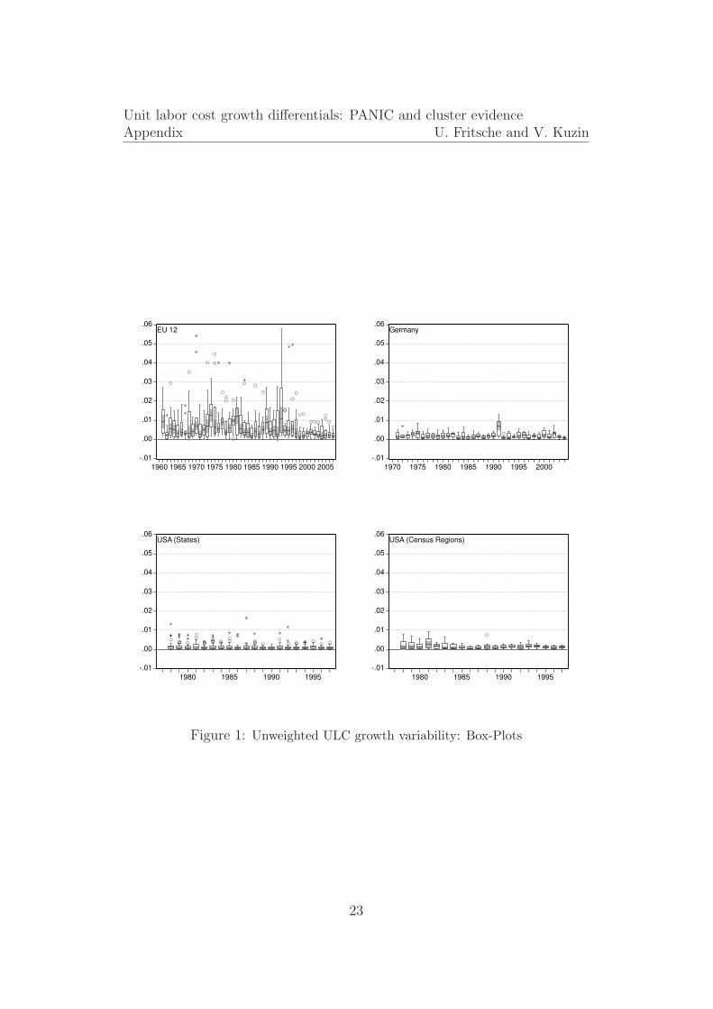
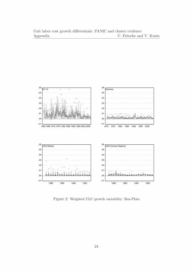
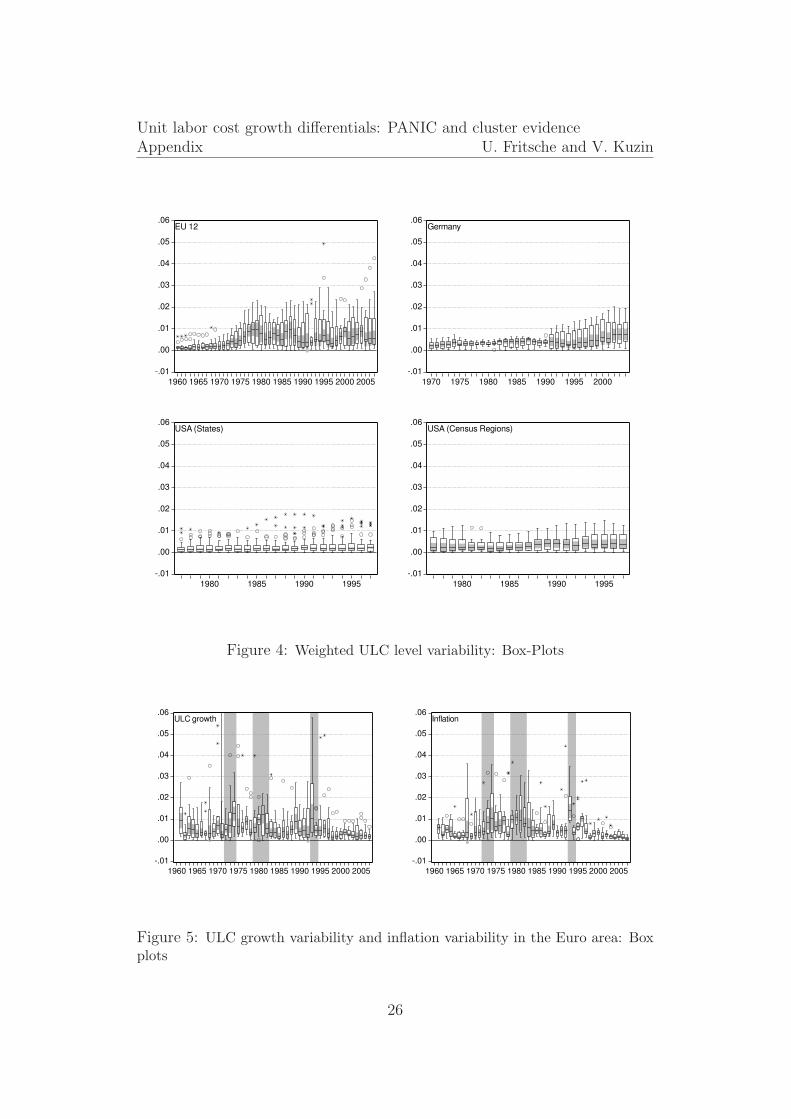
We calculated unweighted (j = 1/N) as well as real GDP weighted (j =GDPj/GDP ∗) variability measures for levels and growth rates. The respec-tive cross-section distributions of sj for each year are plotted using Box-Plots

1This, in turn became an argument in statements of ECB officials quite recently: “[I]nmost countries [of the Euro area], domestic factors dominate external factors in generatinginflation differentials. In particular, we have witnessed a sustained divergence of wagedevelopments across the euro area, and narrower differences in labour productivity growth.As a result, differentials in the growth of unit labour costs have been persistent.”(Trichet,2006

1


2 for the Euro area (EU 12), Germany, the United States (States and Censusregions). 3

First, we look at the cross-section dispersion in ULC growth rates:

Insert figures 1 and 2 about here.

As can be seen in figures 1 and 2, the dispersion was high after the EMS crisisin the early 1990s and diminished in the process of accession to EMU. If welook at the evidence in other currency areas, we notice a historically higherdispersion in ULC growth in Europe than in Germany or the US – whichremains slightly higher also after the introduction of a common currency.

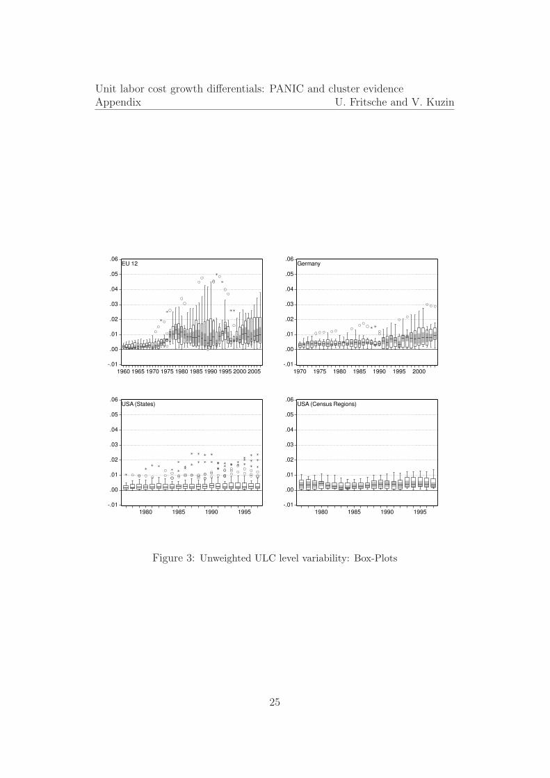
Second, we look at variability measure in ULC levels. The result is some-what different:

Insert figures 3 and 4 about here.

For the EU 12 countries after 1999, level dispersion increased and is nowadaysas high as it was in the early 1990s – at least when considering the weightedmeasure. This is mainly due to the relative large weights of deviations inULC from average in relatively large countries like Spain or Germany. Therespective dispersion data for the panel of Western German Lander show aremarkable increase in both – unweighted and weighted – dispersion measuressince the re-unification boom, however dispersion is not as high as in theEMU. For the United States – irrespective if we have a look at the stateslevel or at a higher level of aggregation (e.g. Census regions) and irrespectivefrom the weigting scheme – the exercise reveals a very stable dispersion ofunit labor cost growth over time.

Last, we compare the calculated measure for ULC growth and inflationto illustrate that there is a relationship between both measures:

Insert figure 5 about here.

The figure reveals, that both – inflation and ULC growth – dispersion mea-sures show peaks around the same periods. Remarkable increases can be

2The median is plotted by a line in the center of a box together with shaded areasdenoting a significance area, a box denoting the borders to the first and third quartile,and a whisker denoting the inner fences (1.5 times the interquartile range). Data pointswith a circle denote near outliers, stars indicate a far outlier.

3See section 3 for details.

2


associated with the two oil price shocks of the 1970s/1980s and the EMScrisis in the early 1990s (shaded areas).

Analyzing the topics of diverging unit labor costs dynamics in a commoncurrency area needs some theoretical underpinnings. It seems to be appro-priate to refer to the concepts of β- and σ-convergence, when analyzing thetopic. According to Barro and Sala-i-Martin (1991), β-convergence is presentif different cross-sectional time series show a mean reverting behavior to acommon level. In contrast, σ-convergence measures the reduction of the over-all dispersion of the time series. As pointed out by Quah (1993), the absenceof σ-convergence – as we see from figures 3 and 4 can not be taken as indicat-ing the absence of β-convergence. In the following, we will mainly base ourarguments on β-convergence. A further distinction, which has to be consid-ered in the context of convergence analysis refers to the distinction betweenabsolute and relative convergence (Bernard and Durlauf, 1996). Absoluteconvergence implies, that the ULC growth rates converge towards the samerate, whereas relative convergence means that the relative distance betweenthe growth rates is stationary. This distinction has important implicationswhen applied to inflation rates: relative convergence within a currency unionimplies, that the competitive position of each country/ region deteriorateson average with a stable rate, whereas absolute convergence implies a stabi-lization of the competitive position at a given point. Such a situation mightbe indicated by comparing the dispersion in levels and growth rates for theEMU.

In general, there are several ways to test for β-convergence empirically.One line of research aims to estimate the average growth rate as a function ofthe deviation from equilibrium at a given starting point (Beck et al., 2006).A second line of research analyzes common trends between inflation (or – inour case – ULC growth rates) in levels within a cointegration framework ase.g in Mentz and Sebastian (2003). A third line of research is based on theanalysis of the stationarity properties of inflation differentials (Beck et al.,2006, Busetti et al., 2006).

As preliminary unit root tests – see the results in section 2.2 – indicate,the ULC level data can best be described as I(2) processes. However to avoida more complicated I(2) analysis and to deliver comparable results with theexiting literature on inflation differentials, we decided to analyze the ULCdata in growth rates.

To get a better understanding of the sources of underlying divergence, weadd therefore to the existing literature on inflation divergence in the followingway:

3


• First, we employ the PANIC approach as developed in Bai and Ng(2004) and used to analyze comovement and heterogeneity in Euroarea data by Eickmeier (2006). The question of interest refers to thedistinction of common and idiosyncratic factors driving the variance inpanels of ULC growth dynamics. If the non-stationarity in the panel ismainly due to common factors but not to the idiosyncratic components,we cannot reject the hypothesis of convergence.

• As a second approach, we analyze the case for convergence clusters(clubs), using the procedure of Hobijn and Franses (2000) based on allpossible bivariate ULC growth rate differentials.

• Third, we aim to make sense out of the factor analysis by means ofan SVAR approach using long-run restrictions (Blanchard and Quah,1989).

• In general, we compare the the evidence for the EMU countries underall methods with the evidence for the States and census regions of theUnited States of America as well as the German Lander.

Our results point to the clearly identifiable existence of one non-stationaryand one stationary common factor for Germany and the United States. Thisis in line with the hypothesis of β-convergence around common factors (whichcould e.g. be associated by country-wide factors like supply or demand shockslike oil price hikes or monetary policy actions) for those countries. For theEuro area, however, it is quite difficult to identify common factors – idiosyn-cratic factors dominate in explaining the bulk of variance – and clusteringseems to be present. The idiosyncratic components in all currency areas arefound to be stationary – however the respective persistence properties arequite different. Wheras in the case of Germany and the US, idiosyncraticcomponents show a white noise behaviour, in the case of EU 12 we find strongserial correlation.

The paper is organized as follows. Having introduced the topic in section1, in section 2 the applied methods are explained and the results presented.Section 3 discusses and summarizes the findings.

4

Unit labor cost growth differentials: PANIC and cluster evidence2 Empirical analysis U. Fritsche and V. Kuzin

2 Empirical analysis

2.1 Data

The data refer to nominal unit labor costs, defined as the ratio of a nominalcompensation of employees numbers to the respective real gross domestic -or gross state - product numbers.4 All data are annual data – however theavailable time span differs a lot. The longest available data set covers theEMU countries. The data (1960 to 2007 as we included the commissionsforecast as two extra data points) are directly available from the AMECOdata base of the EU commission.5

For Germany, the numbers were calculated using the data from the web-site of the Lander’s network for economic statistics (“Arbeitskreis VGR derLander”).6 Unit labour costs have been computed by dividing the (nominal)compensation for employees by the real gross regional product for each of the11 Lander. The SNA classification was changed quite recently in Germanyand the backward calculated numbers cover the time span from 1970 to 2004only. As the data for the old federal republic is only available until 1990, andfrom 1991 only data for all of Germany is provided, the pan-German unitlabour cost index is calculated from the old Lander data until 1990 and frompan-German data from 1991 onwards.

For the United States, the necessary data on gross state products and to-tal compensation of employees has been taken from the Bureau of EconomicAnalysis’ database on regional and state GSP.7 The change from the SICindustrial classification to the NAICS classification in 1997 has created how-ever a slight problem: As data on employees’ compensations has not beenpublished for the first years after the statistical change and have only beenresumed in 2001, the time series can only be constructed from 1977 to 1997.

Last but not least, to calculate the inflation rate variability for EMU (seefigure 5), we used the private consumption deflator as available in AMECO).

4We thank Sebastian Dullien for making his data available.5Please follow the link.6Please follow the link.7Please follow the link.

5

http://ec.europa.eu/economy_finance/indicators/annual_macro_economic_database/ameco_en.htm

http://www.vgrdl.de

http://www.bea.gov/bea/regional/gsp.htm


2.2 Determining the order of integration

Before starting with our convergence investigation, we conducted an analysisof the stationarity properties of the time series under investigation. Weconsidered the following tests:8

• Tests based on a common unit root process: here the methods ofLevin et al. (2002) and Breitung (2000) were considered.

• Tests based on individual unit roots: here an augmented Dickey and Fuller(1979) test and an Phillips and Perron (1988) test in panel versions asproposed by Maddala and Wu (1999) and Choi (2001) were considered.

• All the tests mentioned before are based on the null of a unit root.However we furthermore considered the test described by Hadri (2000),which is based on the null of no unit root.

Table 1 summarize the results.

Insert table 1 about here.

Considering the contradictory results when comparing the tests with oppos-ing null hypotheses, the overall evidence can be interpreted as in favour ofa level of integration higher than 1 for nominal unit labor costs. This is notsurprising, since several studies found I(2) properties for nominal variables(Juselius, 1999). This calls for an I(2) analysis of ULC level convergence –which we leave for a further paper. For the further conduct of this study, wedecided to analyze the convergence issue in terms of ULC growth rates – avariable which is at highest I(1). The reasoning is twofold: on the one handthere is a direct link to the discussion about appropriateness of a uniqueEMU wide inflation rate as the target of monetary policy of the ECB withinthe Euro area and on the other hand this makes our results comparablewith existing studies dealing with inflation differentials in currency unions(Mentz and Sebastian, 2003, Beck et al., 2006, Busetti et al., 2006).

8The panel unit root tests were performed using EViews 5.1 and the respective stan-dard settings with regard to lag length (BIC) and bandwidth selection (Newey-West usingBartlett kernel).

6


2.3 A PANIC attack on ULC growth rates

Bai and Ng (2004) suggest a very useful approach to test for panel unit rootsin the presence of stationary or nonstationary common components, knownas PANIC – Panel Analysis of Nonstationarity in the Idiosyncratic and Com-mon components. PANIC approach allows both idiosyncratic and commoncomponents to be integrated of order one, which makes it very flexible in test-ing panel unit roots. Since we investigate growth rates of unit labor costs,we assume a model with an intercept but without linear trend and followingthe notation of Bai and Ng (2004) our model is:

Xit = ci + λ′

iFt + eit (2)

where Xit are i = 1, . . . , N observed growth rates, Ft is an unobserved vectorof common factors and eit are unit specific idiosyncratic components. BothFt and eit are allowed to be I(1) and for this reason the model has to beestimated in differences, where xit = ∆Xit, ft = ∆Ft and zit = ∆eit, so weestimate the model:

xit = λ′

ift + zit (3)

employing the method of principal components. However, we standard-ize the first differences before estimating in order to avoid possible distor-tions by volatile series in calculating principal components, see Bai and Ng(2001). In particular, we divide differenced time series by their cross em-pirical cross-sectional standard deviations. Estimated common factors andidiosyncratic components are then obtained via cumulating for t = 2, . . . , Tand i = 1, . . . , N

eit =t∑

s=2

zis (4)

Fit =t∑

s=2

fs (5)

where zit = xit − λ′

ifi are estimated residuals. Bai and Ng (2004) show thatestimated factors and idiosyncratic components are consistent, in particularT−1/2eit = T−1/2eit+op(1) and T−1/2Ft = T−1/2HFt+op(1), where H is a fullrank matrix. This rate of convergence is fast enough to leave the asymptoticdistribution of the ADF-test unchanged, if applied to estimated series Ft and

7


eit. So we can apply the univariate ADF-test as well as pooled unit root teststo estimated factors and idiosyncratic components respectively. In case ofestimated factors we allow for a constant in a test regression and test withoutany deterministic terms in the panel case of idiosyncratic components.

An important issue regards our sample sizes in terms of T . Due the useof annual data we have relatively few data points, but, on the other side,it is known from simulation studies of Shiller and Perron (1985) and Perron(1989) that the span of the data has more influence on the power of unit roottests than the number of observations. In this respect we posses a typicaldata span for macroeconometric estimation at least for Germany and Europe- more than 30 and 40 years respectively.

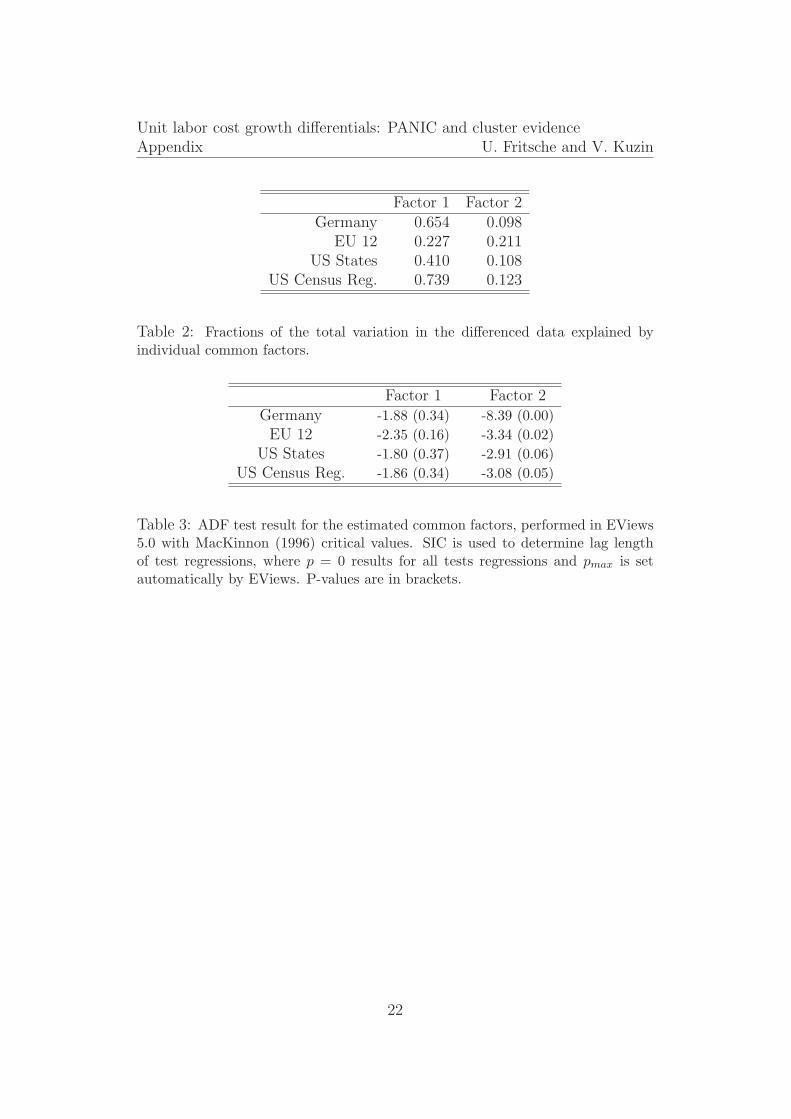
Another important issue is determining the number of factors in PANICframework. Bai and Ng (2002) suggest some information criteria, in particu-lar ICp1, ICp2 and ICp3, to determine the number of factors. But accordinglyto Bai and Ng (2002) our sample size is too small to work with suggested cri-teria and actually there is no closed minima of the criteria (k < kmax) or theychoose too many factors compared to our sample size. Therefore we decidedto calculate fractions of total variation in the differenced data explained byindividual common factors and set k = 2 on the basis of table 2, because thefirst factor explains the main bulk of variance in Germany and the US, andon the other side the two factors are almost equally important in Europe.

Insert table 2 about here.

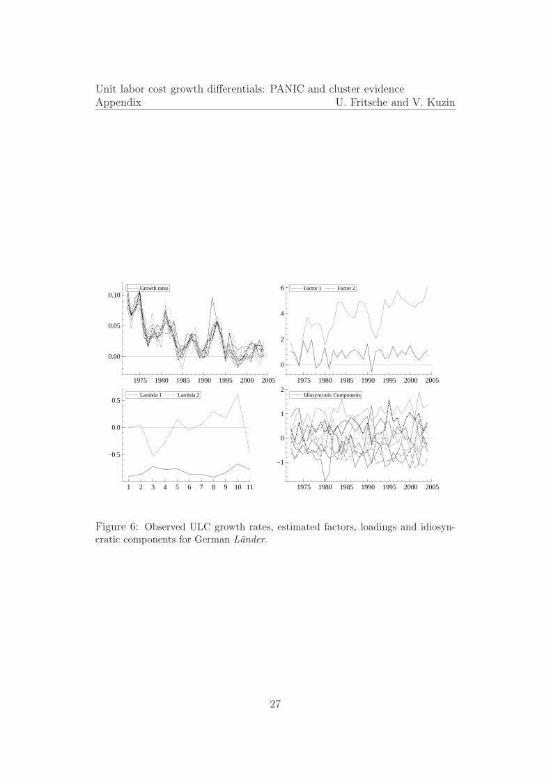
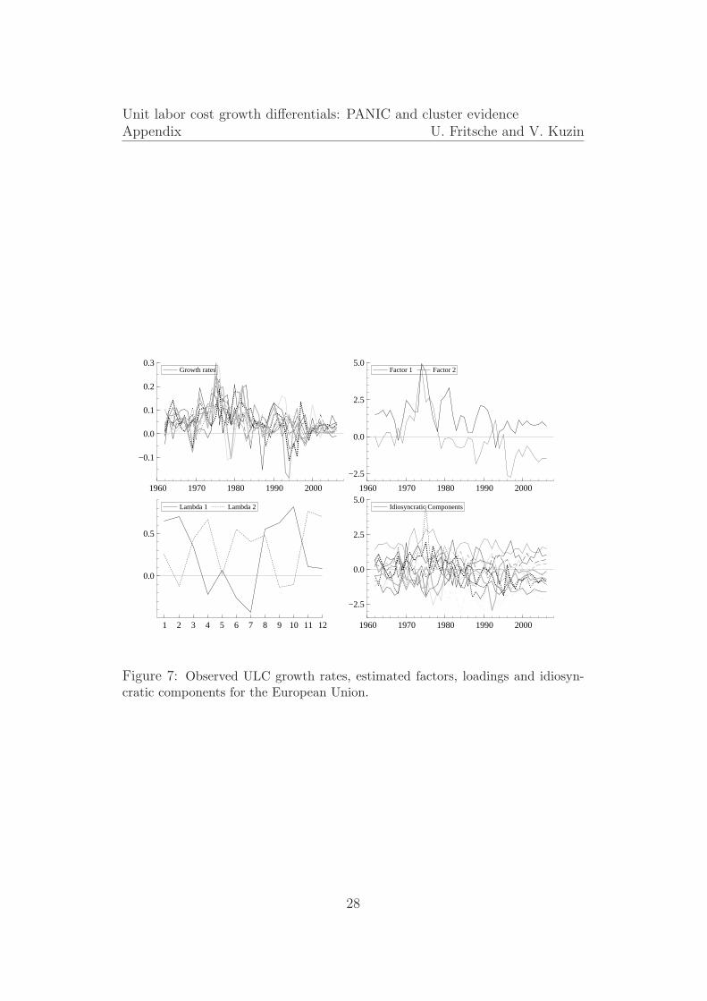
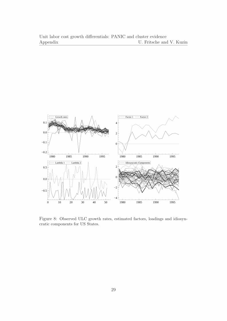
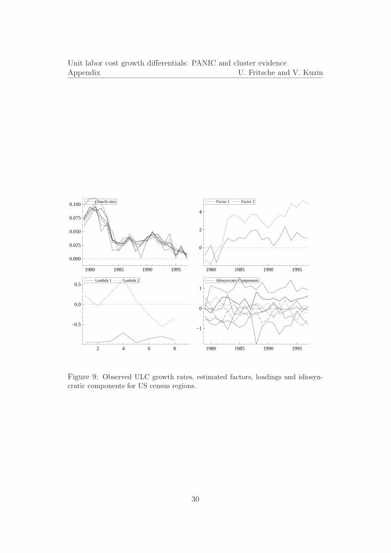
Estimation results for all four panels can be seen in figures 6, 7, 8 and 9.In case of Germany we obtain one factor that has clearly non-stationarypatterns and on the other hand estimated idiosyncratic components lookstationary, see figure 6. Unlike the first picture, there are no clear differencesin patterns of European factors and idiosyncratic components, see figure7. Finally, figures 8 and 9 reveals different patterns between US factorsand idiosyncratic components, where the two estimated factors appear to benon-stationary.

Insert figure 6, 7, 8, and 9 about here.

The visual impression is confirmed by unit root tests. In table 3 we see theresults of ADF tests on estimated common factors. The tests were performedwith EViews 5 by employing the Schwarz information criteria (SIC) to de-termine the lag length. The null of unit root is not rejected for Germany in

8


case of the first factor and is rejected in case of the second one. The testresults for the EU 12 reveal also no rejection of the null for the first factorand rejection for the second factor. Finally, in the US case the first factorturns out to be non-stationary and the null is rejected in the case of thesecond factor at 10% level. However, the small sample size in the US casemakes the reliability of non-panel unit root tests highly questionable.

Furthermore, we perform panel unit root tests for estimated panels of id-iosyncratic components. Two type of tests are calculated: under assumptionof a common unit root process suggested by Levin et al. (2002) as well asby Breitung (2000), and under assumption of individual unit root processesproposed by Maddala and Wu (1999) employing a Fisher-type procedure ofcombining p-values, see table 4. In all cases we employ SIC to select the laglength and Andrews bandwidth selection with quadratic spectral kernel toestimate the long run variances. In all cases we reject the null of panel unitroot. So on the basis of the test results we consider all panels of idiosyncraticcomponents as stationary processes.

Insert tables 3 and 4 about here.

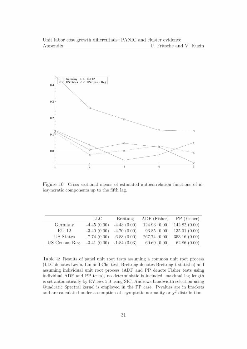
Combining our PANIC evidence with a visual inspection of estimated factorsand idiosyncratic components we conclude that there are a lot of similari-ties between panels of German Lander, US States and US Census Regions.Firstly, in both cases we get at least one non-stationary common factor andstationary idiosyncratic components. Secondly, if we consider the loadingsof this first factor (λ1i, i = 1, . . . , N , see (2)), we observe that they revealnot a lot of variation and always posses the same sign. On the other hand,in the European case many individual idiosyncratic components seem not tobe very different from the common factor itself in terms of variance and alsotheir individual course. It can be also seen if we consider fractions of thetotal variation in the data explained by individual factors, see table 2. Thefraction of the first factor in the European case is quite small, compared tothe results for Germany and the US, and it is almost equal to the fractionof the second factor. Moreover, the individual loadings of the first commonfactor are very different in the case of EU 12. They clearly appear to formclusters. In particular, there are some countries with relatively large positiveloadings and on the other hand units with negative loadings. Last but notleast, we can see differences in the persistence of idiosyncratic components.Figure 10 shows cross sectional means of estimated ACFs of the idiosyncraticcomponents. There is much more persistence in the parts of ULC dynamicsunexplained by common factors than in the US or Germany.

9


Insert figure 10 about here.

2.4 Convergence clubs in ULC growth?

The New Growth Theory allows for the possibility, that countries may notconverge to the same level of per capita GDP, productivity or prices butinstead sub-groups may form convergence clubs. Hobijn and Franses (2000)propose an algorithm for the identification of convergence clubs based onmultivariate stationarity tests. The procedure has recently been applied toregional EMU inflation rates (Busetti et al., 2006). Applying the algorithmusing a version of stationarity test which does not allow for an interceptis equivalent to identifying clusters around the same mean (Busetti et al.,2006, p. 15). The procedures has the nice feature that it is independent ofthe ordering of the series. It is however, not invariant to the number of seriesin that sense that including additional series may change the composition ofclusters.

The clustering algorithm (Hobijn and Franses, 2000, Busetti et al., 2006)is applied to a panel of all possible bivariate differentials in ULC growth ratesand can be described as follows:9

1. Denote ki as a set of indices of variables in cluster i, i ≤ n∗, wheren ≤ n∗ denotes the number of clusters. Define p∗ as a significance levelfor the inclusion of a series in the cluster. Proceed with the followingsteps.

2. Initialize ki = {i} , i = 1, . . . , n = n∗ so that each country/ variable isa cluster.

3. For all i, j ≤ n∗, such that i < j perform a test whether ki ∪ kj

form a cluster according to the criterion of a multivariate stationar-ity test on the contrast (here: by means of a multivariate version of theKwiatkowski et al. (1992) test) and let pi,j the resulting p-value of thetest. Decide: If pi,j > p∗ for all i, j then go to the end of the procedure.

4. Replace cluster ki by ki ∪ kj and drop kj, where i, j correspond to themost likely cluster (maximum p-value of the previous step); replace thenumber of clusters by n∗ − 1 and go one step back.

9The programs for this exercise are available on Bart Hobijn’s homepage. We thankBart Hobijn for helpful comments.

10

http://www.ny.frb.org/research/economists/hobijn/data.html


5. The resulting n∗ clusters are labeled “convergence clubs” (convergenceto a common mean))

6. The procedure proceeds in testing for relative convergence (convergenceto a stationary distance) by applying the same procedure with differentp-values.

Due to comptutational errors – probably due to the fact, that the cross-sectional dimension is much larger in this case than the time dimension –we were not able to conduct the test for the US states, however, we appliedthe procedure succesfully for the US census regions. For all tests, we applieda p-value of 0.01 and a bandwidth of 4 for the Bartlett window used toperform the Kwiatkowski et al. (1992) test. The results are however robustwith regard to the choice of p-value.10

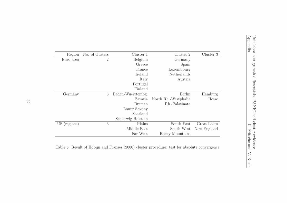
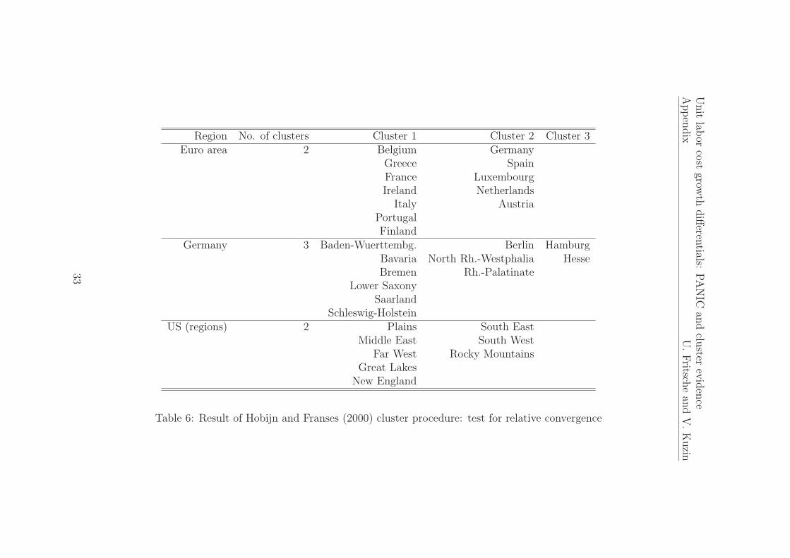
The tables 5 and 6 summarize the result.

Insert table 5 and table 6 about here.

There is evidence for 2, respective 3 clusters in the United States, 3 clusters inGermany and 2 cluster in EU 12. There is furthermore no difference betweenthe results for absolute and relative clustering with the exception of the UScensus regions.11 We can learn two things from the exercise: First, even inestablished currency regions we can find evidence for convergence clusteringand the existence of stable clusters does not per se hinder the functioning ofa currency area.

Second, the clusters in EMU confirms the finding that historically therewas a “hard currency” block – lead by Germany – where countries like Aus-tria or Netherlands were anchored too and a “soft currency” block (mainlyall other countries). Quite astonishing is the finding that Spain is counted asa member of the “hard currency” club. However, looking at the data revealsthat Spain for long periods “overshot” the criterion for being a member inthe “good boys club” in terms of more inflationary policy, a strategy whichwas however from time to time interrupted by sharp (nominal) devaluations.Seen over a long period, this is in line with the hypothesis of absolute con-vergence. It might create a problem however if the mechanisms of (nominal)devaluation are not available anymore and the real exchange rate has toadjust by differences in inflation rates only.

10We did not experiment with the bandwidth, since the value was proposed in the paperof Hobijn and Franses (2000).

11This can be interpreted as evidence for absolute convergence clusters, because each ofthem is a relative convergence cluster with a stationary distance of zero as well.

11


2.5 A structural interpretation of factors driving ULC

growth

It is a well-known drawback of the principal component method, that thefactors stemming from this analysis are not identified in a structural way.However, we can try to identify the structural shocks driving the dynamicsin the panel of ULC growth rates indirectly. To do so, we rely on long-run re-striction in a structural VAR framework as proposed by Blanchard and Quah(1989).

For each panel with i entities, we estimate i unrestricted VARs, consistingof the two estimated common factors, and the ULC growth rate of entity i inthe respective panel. Due to the very few data points, in all cases we allowed2 lags to enter – without a rigorous testing.

To identify the shocks, we assume, that the first common factor – whichis tested to be non-stationary in all cases – is the driving force of non-stationarity (we can e.g. think of a permanent shock which hits the wholecurrency area) and therefore not affected by any other variable in the long-run. Furthermore we assume, that the second factor (we can e.g. thinkof a non-permanent but possibly long-lasting shock hitting the whole cur-rency area) is not affected by country-specific (idiosyncratic) factors in thelong-run.12

Assuming a lag order of one for reasons of simplicity, the structural modelcan be formulated as:

BXt = Γ0 + Γ1Xt−1 + εt ε ∼ N(0, Σε). (6)

The estimated reduced form VAR takes the form:

Xt = A0 + A1Xt−1 + et e ∼ N(0, Σe) (7)

with A0 = B−1Γ0, A1 = B−1Γ1 and et = B−1εt. To identify the VAR, were-write the process in the following moving average representation:

Xt = µ + C(L)εt (8)

12Formally, in the case of EMU, the second factor was found to be non-stationary. Inall other cases, the second factor was found to be stationary. However, due to the difficultproperties of unit root test in small sample cases, we decided to deal with all panels andVARs equally.

12


with µ = [I − (B−1Γ1) L]−1

B−1Γ0 and C(L) = [I − (B−1Γ1) L]−1

B−1 =∞∑i=0

Ai1B

−1Li =∞∑

k=0

C(k)Lk.

We follow the way proposed by Blanchard and Quah (1989) and imposen(n+1)/2 restrictions by the assumption of the orthonormality of the struc-tural innovations: that means Σε = I and n(n − 1)/2 long-run restrictions.The matrix of long-run multipliers C(1) for each of the VARs takes the fol-lowing form:

∆F1

∆F2

∆ULCi

=

C11(1) 0 0C21(1) C22(1) 0C31(1) C32(1) C33(1)

ε1

ε2

ε3

(9)

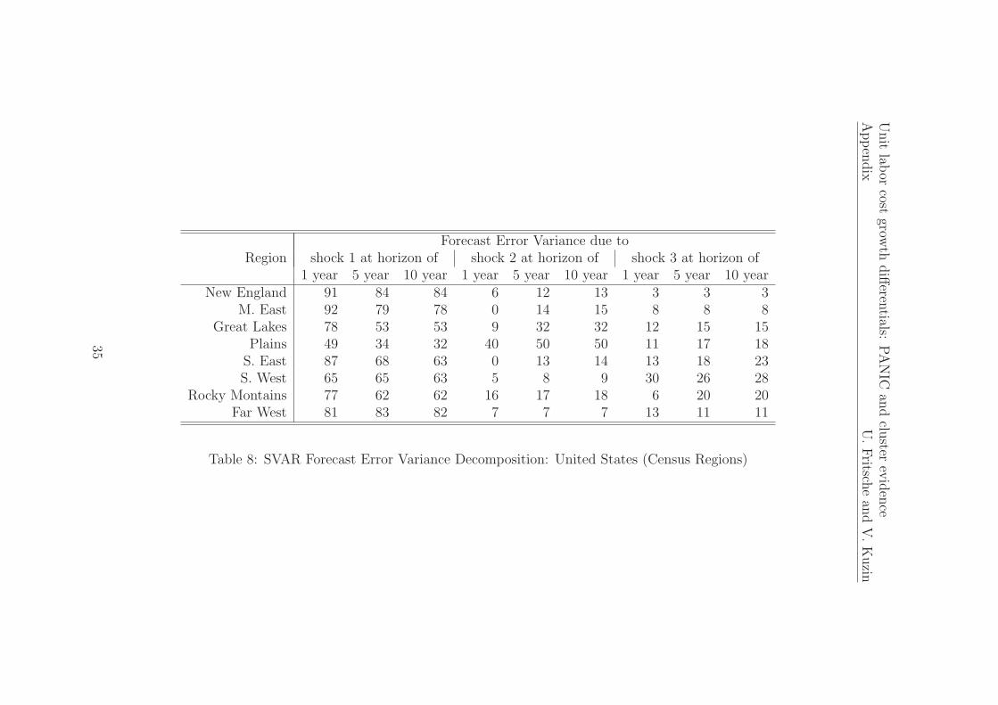
To analyze the issue of convergence, we used forecast error variance decom-positions (FEVD) of the structurally identified VARs. At different forecasthorizons, the FEVD give answer to the question, which portion (in per cent)of the variance of the time series’ stochastic part can be explained by eachof the structural shocks. Specifically we report evidence, how much of thevariance in individual ULC growth rates can be explained either by the firststructural shock (ε1)– which has the highest degree of exogeneity since it isnot affected by any other shocks in the long run –, or by the second structuralshock (ε2)– which is not affected by country-specific effects in the long run–, or by the country-specific shock (ε3)itself.

13

In case of convergence – in the traditional sense, not in the sense ofconvergence clubs – , we would expect the variance in the panel of timeseries to be very much driven by exogenous permanent shocks which areinfluencing each of the panel members in the same way. In contrast, inthe case of convergence clubs or divergence, we could have the finding, thatdifferent panel members are driven by different forces – might this either bedifferent common factors or idiosyncratic factors.

The results are shown in tables 7, 8, and 9.14

Insert tables 7, 8, and 9 about here.

In the case of Germany and the US, we confirm the findings from the PANICanalysis. The variance of the individual ULC growth rates is mainly driven

13Given the limited number of observations, the point estimates might be misleading.However, we did not bootstrap confidence bounds since the interest is more in the generalpicture instead of assessing the uncertainty around the point estimates.

14Again we skip the results for the US federal states. These results are available fromthe authors on request.

13

Unit labor cost growth differentials: PANIC and cluster evidence3 Discussion U. Fritsche and V. Kuzin

by the first common factor – which is in line with the hypothesis of conver-gence. There are some exceptions, where either the second factor and/ orthe idiosyncratic shock seems to play a role but these cases are exceptionsrather than the rule.

In the case of EMU, we however find very differing effects of the shockson ULC growth rate variance for different panel members. In some countries,the variance to a considerable extent driven by the first shock (e.g. Belgium,Germany, Luxemburg, Netherlands, Austria) – which seems to grasp lastingshocks to the hard currency club. Other countries are much more connectedto the second shock (e.g. Greece, Spain, Portugal, Ireland, Finland) – whichseems to grasp common movements in catching-up countries. All in all, thevariance explained by idiosyncratic shocks is much higher than in the USor Germany. These results are in line with the high dispersion in the factorloadings in the PANIC analysis and the relatively high persistence of idiosyn-cratic components compared to the US and Germany. More specifically, wecan confirm to some extent the result from the convergence club analysis.

3 Discussion

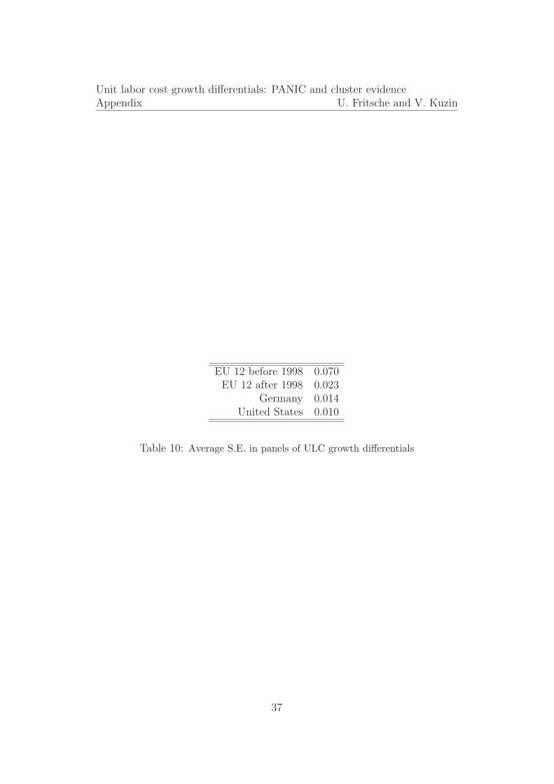
Our analysis of ULC growth dynamics in selected countries/ regions pointsto the existence of one non-stationary common factor for the United States(States and Census regions) and Germany. The idiosyncratic componentsin all currency areas are found to be stationary. This is in line with thehypothesis of β-convergence around common factors (which could e.g. be as-sociated by country-wide factors like supply or demand shocks like oil pricehikes or monetary policy actions). For the Euro area, however, it is quitedifficult to identify common factors – idiosyncratic factors dominate in ex-plaining the bulk of variance – and clustering seems to be present. It cannotbe rejected that idiosyncratic factors in the Euro area are stationary, howeverthe persistence is much stronger than in other currency areas – which pointsto long-lasting adjustment processes. There is little sign of change in thatrespect in the second half of the sample. The case for convergence clusters isconfirmed when using the procedure as in Hobijn and Franses (2000) for allcurrency areas. The differences between individual ULC growth rates are,however, much smaller for the United States and Germany than within theEU 12 (table 10).

These results were confirmed by an SVAR analysis to give the unidentifiedfactors a more structural interpretation. Forecast error variance decompo-

14


sition reveals that for the United States and Germany one non-stationarycommon factor can be identified as the main source of forecast error varianceof almost all individual ULC growth rates. The picture differs dramaticallywith regard to the EMU countries. Here, the finding is more in line with theexistence of convergence clubs and a very strong influence of idiosyncraticcomponents.

Why should a central bank like the ECB be concerned about this finding?Prices in one country would be a little higher than in the rest of the unionfor a number of years and below the average for another number of years.The phenomenon, one could argue, is a purely nominal one. However, thereare a number of theoretical arguments to cast doubt on this view. Instead, ifdivergences persist for a prolonged periods, they might cause misallocationsand even long-term detrimental effects to growth. There are different reasonsfor that: Domestic inflation makes the financing of consumption and capitalinput cheaper while investment in the tradable sector becomes less attrac-tive with the loss of competitiveness, it might lead to excessive investmentin the housing sector – especially if financial markets are incomplete andsuffer from asymmetric information problems. Not only might an excessiveamount of capital be allocated to this sector which contributes relatively littleto long-term productivity growth but thus might shift the Beveridge curveoutwards and increase structural (long-term) unemployment. Furthermore,persistent deviations in the price trend might lead to a strong overvaluationof one country within the monetary union. Whereas undervaluation leadsto increasing exports and income, increasing import prices lead to a dete-rioration in the trade balance and adjustment occurs in the long run – asthe exchange rate channel dominates the interest rate channel. Adjustmentprocesses might however be asymmetric with regard to speed and intensity,due to hysteresis phenonenom: Once trapped in a situation of overvaluation,profits might suffer and investment contract, leading to a longer period of sub-trend economic growth until the real appreciation is corrected again. Theseboom-and-bust-periods might not only bring about negative welfare effectsdue to increased income volatility but might also lower the potential outputof a single country if there are good arguments for hysteresis in the labourmarket, meaning that unemployment is at least to a certain extent path-dependent (Fritsche and Logeay, 2002, Gottschalk and Fritsche, 2005). Lastbut not least, political economy arguments hint that prolonged boom-and-bust cycles as a result from divergences might actually endanger the politicalstability of the euro-area. Leaving the union would allow the country to de-preciate sharply and forego the adjustment costs of relative wage deflation.If the country’s politicians have a sufficiently high personal discount rate, the

15


short-term benefits of leaving EMU might actually be perceived larger thanthe long-run costs of the forgone membership in the monetary union such aslower long-term interest rates. This might in the end lead to single countriespulling out of EMU.

One might argue, that the perceived results might be due to the timespan under investigation. Due to a lack of evidence after the introductionof the Euro and given the existence of long-lasting adjustment processes, wecan only informally test for structural change. However, preliminary stabilityinvestigations as well as a visual inspection of the factor decomposition anal-ysis results gives rise to serious concern for the Euro area. The behaviour ofidiosyncratic components does not seem to have changed and shows strongpersistence. The same is true when looking at the cluster procedure results– there is still evidence for inflation clubs in the EMU (12). This findingis in line with the findings of Busetti et al. (2006) – where in contrast toour study monthly inflation numbers were used. The discussion has clearimplications for the conduct of economic policy within the Euro area. Thelasting evidence for persistent inflation differentials calls for re-organizationof macroeconomic policy at a European level – e.g. newly designed fiscaltransfer mechanisms or wage policy coordination (Fritsche et al., 2005)– orfor increased labor mobility and productivity adjustment (Belke and Gros,2006, Blanchard, 2006). Both solution have their own advantages and draw-backs – which goes beyond the scope of this paper.

16

Unit labor cost growth differentials: PANIC and cluster evidenceReferences U. Fritsche and V. Kuzin

References

Alvarez, L., E. Dhyne, M. Hoeberichts, C. Kwapil, H. Le Bihan,

P. Lunnemann, F. Martins, R. Sabbatini, H. Stahl, Ph. Ver-

meulen, and J. Vilmunen, “Sticky prices in the euro area: a sum-mary of new micro evidence,” Discussion Paper Series 1: Economic Studies02/2006, Deutsche Bundesbank 2006.

Angeloni, I. and M. Ehrmann, “Euro area inflation differentials,” Work-ing Paper Series 388, European Central Bank 2004.

, L. Aucremanne, M. Ehrmann, J. Gali, A. Levin, and F. Smets,“New evidence on inflation persistence and price stickiness in the Euroarea: Implications for macro modelling,” Journal of the European Eco-nomic Association, 2006, 4, 562–574.

Bai, J. and S. Ng, “A PANIC Attack on Unit Roots and Cointegration,”Boston College Working Papers in Economics 519, Boston College Depart-ment of Economics 2001.

and , “Determining the numbers of factors in approximate factor mod-els,” Econometrica, 2002, 70, 191–221.

and , “A PANIC attack on unit roots and cointegration,” Econometrica,2004, 72, 1127–1177.

Barro, R. and X. Sala-i-Martin, “Convergence across states and regions,”Brookings Papers on Economic Activity, 1991, 1991 (1), 107–182.

Beck, G., K. Hubrich, and M. Marcellino, “Regional Inflation Dynam-ics within and across Euro Area Countries and a Comparison with theUS,” Technical Report 2006.

Belke, A. and D. Gros, “Instability of the Eurozone? On Monetary Policy,House Prices and Structural Reforms,” Hohenheimer Diskussionsbeitrageaus dem Institut fr Volkswirtschaftslehre (520) 271/2006, Universitat Ho-henheim, Stuttgart 2006.

Benigno, P. and David Lopez-Salido, “Inflation persistence and optimalmonetary policy in the Euro area,” Working Paper Series 178, EuropeanCentral Bank 2002.

Bernard, A. B. and S. N. Durlauf, “Interpreting tests of the convergencehypothesis,” Journal of Econometrics, 1996, 71, 161–173.

17


Blanchard, O., “Adjustment Within the Euro: The Difficult Case of Por-tugal,” MIT Department of Economics Working Paper 06-04, MIT 2006.

and D. Quah, “The Dynamic Effects of Aggregate Demand and Ag-gregate Supply Disturbances,” American Economic Review, 1989, 79 (4),655–673.

Breitung, J., “The Local Power of Some Unit Root Tests for Panel Data,” inB. Baltagi, ed., Nonstationary Panels, Panel Cointegration, and DynamicPanels, Vol. 15 of Advances in Econometrics, Amsterdam: JAI Press, 2000,pp. 161–178.

Busetti, F., L. Forni, A. Harvey, and F. Venditti, “Inflation conver-gence and divergence within the European Monetary Union,” ECB Work-ing Paper Series 574, European Central Bank 2006.

Campolmi, A. and E. Faia, “Cyclical inflation divergence and differentlabor market institutions in the EMU.,” Working Paper Series 619, Euro-pean Central Bank 2006.

Cecchetti, S. G. and G. Debelle, “Has the inflation process changed?,”Economic Policy, 2006, 46, 313–351.

Choi, I., “Unit Root Tests for Panel Data,” Journal of International Moneyand Finance, 2001, 20, 249–272.

Dickey, D.A. and W.A. Fuller, “Distribution of the Estimators for Au-toregressive Time Series with a Unit Root,” Journal of the American Sta-tistical Association, 1979, 74, 427–431.

Eickmeier, S., “Comovements and heterogeneity in the euro area analyzedin a non-stationary dynamic factor model,” Deutsche Bundesbank Discus-sion Paper Series 1: Economic Studies 31, Deutsche Bundesbank 2006.

European Central Bank, “Monetary policy and inflation differentials in aheterogenous currency area,” Monthly Bulletin, 2005, 05/2005, 61–77.

Fritsche, U. and C. Logeay, “Structural Unemployment and Output Gapin Germany: Evidence from an SVAR Analysis within a Hysteresis Frame-work,” DIW Discussion Paper 312, DIW Berlin, Berlin 2002.

, , K. Lommatzsch, K. Rietzler, S. Stephan, R. Zwiener,

C. Kiziltepe, and Ch. Proano Acosta, “Auswirkungen von

18


landerspezifischen Differenzen in der Lohn-, Preisniveau und Produk-tivitatsentwicklung auf Wachstum und Beschaftigung in den Landern desEuroraums,” Politikberatung kompakt 08/2005, Deutsches Institut furWirtschaftsforschung (DIW Berlin) 2005.

Gonzalez-Paramo, J. M., “Regional divergence in the euro area,” 2005.Speech by Jose Manuel Gonzalez-Paramo, Member of the Executive Boardof the ECB, International Conference on “The Role of Government inRegional Economic Development”, REDE (Research in Economics, Energyand the Environment), Universidade de Vigo, Baiona, 19 September 2005.

Gottschalk, J. and U. Fritsche, “The New Keynesian Model and the long-run vertical Phillips Curve: Does it hold for Germany?,” DIW DiscussionPaper 521, DIW Berlin, Berlin 2005.

Hadri, K., “Testing for Stationarity in Heterogeneous Panel Data,” Econo-metric Journal, 2000, 3, 148–161.

Hobijn, B. and Ph. H. Franses, “Asymptotically perfect and relativeconvergence of productivity,” Journal of Applied Econometrics, 2000, 15,59–81.

Im, K.S., M.H. Pesaran, and Y. Shin, “Testing for unit roots in het-erogenous panels,” Journal of Econometrics, 2003, 115, 53–74.

Issing, O., “One size fits all! A single monetary policy for the euro area,”2005. Speech by Otmar Issing, Member of the Executive Board of the ECBInternational Research Forum, Frankfurt am Main, 20 May 2005.

Juselius, K., “Price convergence in the long run and the medium run. AnI(2) analysis of six price indices,” in R. Engle and H White, eds., Cointe-gration, Causality, and Forecasting: Festschrift in Honour of Clive W.J.Granger, Oxford University Press, 1999, chapter 13.

Kwiatkowski, D., P. Phillips, P. Schmidt, and Y. Shin, “Testingthe null hypothesis of stationarity against the alternative of a unit root,”Journal of Econometrics, 1992, 54, 159–178.

Lane, Ph., “The real effects of EMU,” Discussion Paper Series 5536, CEPR2006.

Levin, A., C.-F. Lin, and C.-S. Chu, “Unit root tests in panel data:Asymptotic and finite sample properties,” Journal of Econometrics, 2002,108, 1–24.

19


MacKinnon, J. G., “Numerical Distribution Functions for Unit Root andCointegration Tests,” Journal of Applied Econometrics, 1996, 11, 601–618.

Maddala, G. S. and S. Wu, “A Comparative Study of Unit Root Testswith Panel Data and A New Simple Test,” Oxford Bulletin of Economicsand Statistics, 1999, 61, 631–52.

Mentz, M. and S. P. Sebastian, “Inflation convergence after the intro-duction of the Euro,” CFS Working Paper 2003/30, Center for FinancialSudies an der Johann Wolfgang Goethe-Universitat 2003.

Perron, P., “Testing for a random walk: A simulation experiment when thesampling interval is varied,” in B. Raj, ed., Advances in econometrics andmodelling, Dordrecht: Kluwer, 1989.

Phillips, P.C.B. and P. Perron, “Testing for a Unit Root in Time SeriesRegression,” Biometrika, 1988, 75, 335–346.

Quah, D.T., “Galton’s fallacy and tests of the convergence hypothesis.,”The Scandinavian Journal of Economics, 1993, 95, 427–443.

Shiller, R. J. and P. Perron, “Testing the random walk hypothesis: Powerversus frequency of observation,” Economic Letters, 1985, 18, 381–386.

Trichet, J. C., “Economic integration in the euro area,” BIS Review, 2006,27, 1–7. Speech by Mr Jean-Claude Trichet, President of the EuropeanCentral Bank, at the 15th European Regional Conference of the Board ofGovernors, Tel Aviv University, Paris, 31 March 2006.

20

Unit labor cost growth differentials: PANIC and cluster evidenceAppendix U. Fritsche and V. Kuzin

Appendix

Figures and Tables

Currency areaTest on...

log(y) ∆ log(y) ∆(∆ log(y))p-val. p-val. p-val.

Euro areaLevin et al. (2002) 0.32 0.00 0.00

Breitung (2000) 0.90 0.00 0.00Im et al. (2003) 1.00 0.00 0.00

Dickey and Fuller (1979) (Fisher χ2) 0.99 0.00 0.00

Phillips and Perron (1988) (Fisher χ2) 1.00 0.00 0.00

Hadri (2000) 0.00 0.00 0.73Germany

Levin et al. (2002) 0.00 0.00 0.00Breitung (2000) 1.00 0.00 0.00Im et al. (2003) 0.00 0.00 0.00



Hadri (2000) 0.00 0.00 0.01USA (States)




Hadri (2000) 0.00 0.00 0.72USA (Regions)




Hadri (2000) 0.00 0.00 0.95

Table 1: ULC panel unit root tests

21


Factor 1 Factor 2Germany 0.654 0.098

EU 12 0.227 0.211US States 0.410 0.108

US Census Reg. 0.739 0.123

Table 2: Fractions of the total variation in the differenced data explained byindividual common factors.

Factor 1 Factor 2Germany -1.88 (0.34) -8.39 (0.00)

EU 12 -2.35 (0.16) -3.34 (0.02)

US States -1.80 (0.37) -2.91 (0.06)

US Census Reg. -1.86 (0.34) -3.08 (0.05)

Table 3: ADF test result for the estimated common factors, performed in EViews5.0 with MacKinnon (1996) critical values. SIC is used to determine lag lengthof test regressions, where p = 0 results for all tests regressions and pmax is setautomatically by EViews. P-values are in brackets.

22


-.01

.00

.01

.02

.03

.04

.05

.06

1960 1965 1970 1975 1980 1985 1990 1995 2000 2005

EU 12

-.01

.00

.01

.02

.03

.04

.05

.06

1970 1975 1980 1985 1990 1995 2000

Germany

-.01

.00

.01

.02

.03

.04

.05

.06

1980 1985 1990 1995

USA (States)

-.01

.00

.01

.02

.03

.04

.05

.06

1980 1985 1990 1995

USA (Census Regions)

Figure 1: Unweighted ULC growth variability: Box-Plots

23


-.01

.00

.01

.02

.03

.04

.05

.06

1960 1965 1970 1975 1980 1985 1990 1995 2000 2005

EU 12

-.01

.00

.01

.02

.03

.04

.05

.06

1970 1975 1980 1985 1990 1995 2000

Germany

-.01

.00

.01

.02

.03

.04

.05

.06

1980 1985 1990 1995

USA (States)

-.01

.00

.01

.02

.03

.04

.05

.06

1980 1985 1990 1995


Figure 2: Weighted ULC growth variability: Box-Plots

24


-.01

.00

.01

.02

.03

.04

.05

.06

1960 1965 1970 1975 1980 1985 1990 1995 2000 2005

EU 12

-.01

.00

.01

.02

.03

.04

.05

.06

1970 1975 1980 1985 1990 1995 2000

Germany

-.01

.00

.01

.02

.03

.04

.05

.06

1980 1985 1990 1995

USA (States)

-.01

.00

.01

.02

.03

.04

.05

.06

1980 1985 1990 1995


Figure 3: Unweighted ULC level variability: Box-Plots

25


-.01

.00

.01

.02

.03

.04

.05

.06

1960 1965 1970 1975 1980 1985 1990 1995 2000 2005

EU 12

-.01

.00

.01

.02

.03

.04

.05

.06

1970 1975 1980 1985 1990 1995 2000

Germany

-.01

.00

.01

.02

.03

.04

.05

.06

1980 1985 1990 1995

USA (States)

-.01

.00

.01

.02

.03

.04

.05

.06

1980 1985 1990 1995


Figure 4: Weighted ULC level variability: Box-Plots

-.01

.00

.01

.02

.03

.04

.05

.06

1960 1965 1970 1975 1980 1985 1990 1995 2000 2005

ULC growth

-.01

.00

.01

.02

.03

.04

.05

.06

1960 1965 1970 1975 1980 1985 1990 1995 2000 2005

Inflation

Figure 5: ULC growth variability and inflation variability in the Euro area: Boxplots

26


1975 1980 1985 1990 1995 2000 2005

0.00

0.05

0.10Growth rates

1975 1980 1985 1990 1995 2000 2005

0

2

4

6 Factor 1 Factor 2

1 2 3 4 5 6 7 8 9 10 11

−0.5

0.0

0.5Lambda 1 Lambda 2

1975 1980 1985 1990 1995 2000 2005

−1

0

1

2Idiosyncratic Components

Figure 6: Observed ULC growth rates, estimated factors, loadings and idiosyn-cratic components for German Lander.

27


1960 1970 1980 1990 2000

−0.1

0.0

0.1

0.2

0.3Growth rates

1960 1970 1980 1990 2000

−2.5

0.0

2.5

5.0Factor 1 Factor 2

1 2 3 4 5 6 7 8 9 10 11 12

0.0

0.5

Lambda 1 Lambda 2

1960 1970 1980 1990 2000

−2.5

0.0

2.5

5.0Idiosyncratic Components

Figure 7: Observed ULC growth rates, estimated factors, loadings and idiosyn-cratic components for the European Union.

28


1980 1985 1990 1995

−0.2

−0.1

0.0

0.1

Growth rates

1980 1985 1990 1995

0

2

4

Factor 1 Factor 2

0 10 20 30 40 50

−0.5

0.0

0.5

Lambda 1 Lambda 2

1980 1985 1990 1995

−4

−2

0

2

Idiosyncratic Components

Figure 8: Observed ULC growth rates, estimated factors, loadings and idiosyn-cratic components for US States.

29


1980 1985 1990 1995

0.000

0.025

0.050

0.075

0.100Growth rates

1980 1985 1990 1995

0

2

4

Factor 1 Factor 2

2 4 6 8

−0.5

0.0

0.5Lambda 1 Lambda 2

1980 1985 1990 1995

−1

0

1

Idiosyncratic Components

Figure 9: Observed ULC growth rates, estimated factors, loadings and idiosyn-cratic components for US census regions.

30


1 2 3 4 5

0.0

0.1

0.2

0.3

0.4

Germany US States

EU 12 US Census Reg.

Figure 10: Cross sectional means of estimated autocorrelation functions of id-iosyncratic components up to the fifth lag.

LLC Breitung ADF (Fisher) PP (Fisher)

Germany -4.45 (0.00) -4.43 (0.00) 124.93 (0.00) 142.82 (0.00)

EU 12 -3.40 (0.00) -4.70 (0.00) 93.85 (0.00) 135.01 (0.00)

US States -7.74 (0.00) -6.83 (0.00) 267.74 (0.00) 353.16 (0.00)

US Census Reg. -3.41 (0.00) -1.84 (0.03) 60.69 (0.00) 62.86 (0.00)

Table 4: Results of panel unit root tests assuming a common unit root process(LLC denotes Levin, Lin and Chu test, Breitung denotes Breitung t-statistic) andassuming individual unit root process (ADF and PP denote Fisher tests usingindividual ADF and PP tests), no deterministic is included, maximal lag lengthis set automatically by EViews 5.0 using SIC, Andrews bandwidth selection usingQuadratic Spectral kernel is employed in the PP case. P-values are in bracketsand are calculated under assumption of asymptotic normality or χ

2 distribution.

31

Unit

labor

costgrow

thdiff

erentials:

PA

NIC

and

cluster

evid

ence

Appen

dix

U.Fritsch

ean

dV

.K

uzin

Region No. of clusters Cluster 1 Cluster 2 Cluster 3Euro area 2 Belgium Germany

Greece SpainFrance LuxembourgIreland Netherlands

Italy AustriaPortugalFinland

Germany 3 Baden-Wuerttembg. Berlin HamburgBavaria North Rh.-Westphalia HesseBremen Rh.-Palatinate

Lower SaxonySaarland

Schleswig-HolsteinUS (regions) 3 Plains South East Great Lakes

Middle East South West New EnglandFar West Rocky Mountains

Table 5: Result of Hobijn and Franses (2000) cluster procedure: test for absolute convergence

32

Unit

labor

costgrow

thdiff

erentials:

PA

NIC

and

cluster

evid

ence

Appen

dix

U.Fritsch

ean

dV

.K

uzin

Region No. of clusters Cluster 1 Cluster 2 Cluster 3Euro area 2 Belgium Germany

Greece SpainFrance LuxembourgIreland Netherlands

Italy AustriaPortugalFinland

Germany 3 Baden-Wuerttembg. Berlin HamburgBavaria North Rh.-Westphalia HesseBremen Rh.-Palatinate

Lower SaxonySaarland

Schleswig-HolsteinUS (regions) 2 Plains South East

Middle East South WestFar West Rocky Mountains

Great LakesNew England

Table 6: Result of Hobijn and Franses (2000) cluster procedure: test for relative convergence

33

Unit

labor

costgrow

thdiff

erentials:

PA

NIC

and

cluster

evid

ence

Appen

dix

U.Fritsch

ean

dV

.K

uzin

Forecast Error Variance due toCountry shock 1 at horizon of shock 2 at horizon of shock 3 at horizon of

1 year 5 year 10 year 1 year 5 year 10 year 1 year 5 year 10 yearBaden-Wuerttembg. 86 62 61 0 13 15 13 24 24

Bavaria 80 63 62 0 12 13 20 25 25Berlin 68 66 65 11 15 16 21 19 20

Bremen 44 31 31 9 8 9 47 61 60Hamburg 56 44 44 3 12 12 41 44 44

Hesse 70 67 68 0 10 10 29 23 22Lower Saxony 75 65 65 1 11 11 24 24 24

North Rh.-Westphalia 77 56 56 11 36 36 12 8 8Rh.-Palatinate 66 52 51 1 14 15 33 34 34

Saarland 45 33 32 30 53 54 25 14 14Schleswig-Holstein 70 66 66 8 11 11 22 23 22

Table 7: SVAR Forecast Error Variance Decomposition: Germany

34

Unit

labor

costgrow

thdiff

erentials:

PA

NIC

and

cluster

evid

ence

Appen

dix

U.Fritsch

ean

dV

.K

uzin

Forecast Error Variance due toRegion shock 1 at horizon of shock 2 at horizon of shock 3 at horizon of

1 year 5 year 10 year 1 year 5 year 10 year 1 year 5 year 10 yearNew England 91 84 84 6 12 13 3 3 3

M. East 92 79 78 0 14 15 8 8 8Great Lakes 78 53 53 9 32 32 12 15 15

Plains 49 34 32 40 50 50 11 17 18S. East 87 68 63 0 13 14 13 18 23S. West 65 65 63 5 8 9 30 26 28

Rocky Montains 77 62 62 16 17 18 6 20 20Far West 81 83 82 7 7 7 13 11 11

Table 8: SVAR Forecast Error Variance Decomposition: United States (Census Regions)

35

Unit

labor

costgrow

thdiff

erentials:

PA

NIC

and

cluster

evid

ence

Appen

dix

U.Fritsch

ean

dV

.K

uzin

Forecast Error Variance due toCountry shock 1 at horizon of shock 2 at horizon of shock 3 at horizon of

1 year 5 year 10 year 1 year 5 year 10 year 1 year 5 year 10 yearBelgium 52 52 52 5 8 8 43 40 40

Germany 49 41 40 1 3 3 50 56 56Greece 4 4 4 31 31 31 65 65 65Spain 1 5 5 48 44 43 51 52 52

France 9 10 11 2 33 33 88 57 56Ireland 5 7 7 30 33 33 66 59 59

Italy 31 40 39 15 17 17 55 44 44Luxembourg 45 27 27 12 13 13 43 61 61Netherlands 59 52 51 1 6 6 40 42 42

Austria 75 69 69 1 3 3 24 28 28Portugal 5 12 13 51 54 55 44 33 32Finland 0 1 2 50 42 42 50 56 56

Table 9: SVAR Forecast Error Variance Decomposition: EU 12

36


EU 12 before 1998 0.070EU 12 after 1998 0.023

Germany 0.014United States 0.010

Table 10: Average S.E. in panels of ULC growth differentials

37


Identifier EMU Germany US Census Regions US Federal States

1 Belgium Baden-Wuerttembg. New England Alabama

2 Germany Bavaria Middle East Alaska

3 Greece Berlin Great Lakes Arizona

4 Spain Bremen Plains Arkansas

5 France Hamburg South East California

6 Ireland Hesse South West Colorado

7 Italy Lower Saxony Rocky Montains Connecticut

8 Luxembourg North Rh.-Westphalia Far West Delaware

9 Netherlands Rh.-Palatinate District of Columbia

10 Austria Saarland Florida

11 Portugal Schleswig-Holstein Georgia

12 Finland Hawaii

13 Idaho

14 Illinois

15 Indiana

16 Iowa

17 Kansas

18 Kentucky

19 Louisiana

20 Maine

21 Maryland

22 Massachusetts

23 Michigan

24 Minnesota

25 Mississippi

26 Missouri

27 Montana

28 Nebraska

29 Nevada

30 New Hampshire

31 New Jersey

32 New Mexico

33 New York

34 North Carolina

35 North Dakota

36 Ohio

37 Oklahoma

38 Oregon

39 Pennsylvania

40 Rhode Island

41 South Carolina

42 South Dakota

43 Tennessee

44 Texas

45 Utah

46 Vermont

47 Virginia

48 Washington

49 West Virginia

50 Wisconsin

51 Wyoming

Table 11: Country/ Region identifiers used in figures

38

Documents

Unit Labor Cost Growth Differentials in the Euro Area, Germany, and the US: Lessons from PANIC and Cluster Analysis