Labor Cost and SugarcaneLabor Cost and Sugarcane

Mechanization in Florida:Mechanization in Florida:

NPV and Real Options ApproachNPV and Real Options Approach

Nobuyuki IwaiNobuyuki IwaiRobert D. EmersonRobert D. Emerson

International Agricultural Trade and Policy CenterInternational Agricultural Trade and Policy CenterDepartment of Food and Resource EconomicsDepartment of Food and Resource Economics

University of FloridaUniversity of Florida

BackgroundBackground

!! Foreign workers in US agricultureForeign workers in US agriculture

"" 77% of farm workers in 2002-0477% of farm workers in 2002-04

"" At least 50% of farm workers areAt least 50% of farm workers areundocumented in 2002-04 (undocumented in 2002-04 (16% 1989-91,16% 1989-91,38% in 1993-95)38% in 1993-95)

!! Wage gapWage gap

Average predicted wages for authorized,Average predicted wages for authorized,permanent resident, and citizen worker are permanent resident, and citizen worker are 10%,10%,18% and 14%18% and 14% higher than for unauthorized higher than for unauthorizedworkers (Iwai et al. 2006).workers (Iwai et al. 2006).

Immigration PolicyImmigration Policy Reform Reform

!! Increased border and domesticIncreased border and domesticenforcement, amnesty and guest workerenforcement, amnesty and guest workerprogramsprograms

Goal: Goal: legal labor forcelegal labor force

!! Concern that the reform might lead toConcern that the reform might lead tolabor cost increase in US labor cost increase in US agag..

!! Need to study the impact of labor cost Need to study the impact of labor costincrease: increase: MechanizationMechanization, Termination, Termination(Emerson 2007)(Emerson 2007)

PreviousPrevious Studies on Labor Cost Studies on Labor Costand Sugarcane Mechanizationand Sugarcane Mechanization

!! ZeppZepp and Clayton (1975) found cost advantage and Clayton (1975) found cost advantageof mechanical harvesting operation over hand-of mechanical harvesting operation over hand-cut as early as 72-3 season.cut as early as 72-3 season.

!! Reduced revenue due to large field losses withReduced revenue due to large field losses withmechanical harvesting, resulting in $40.70 lowermechanical harvesting, resulting in $40.70 lowernet returns per acre in comparison to hand-cut.net returns per acre in comparison to hand-cut.

!! If projected 74-5 machinery operating rates hadIf projected 74-5 machinery operating rates hadbeen used, the net returns per acre would havebeen used, the net returns per acre would havebeen about equal (been about equal (ZeppZepp 1975). 1975).

ProblemsProblems

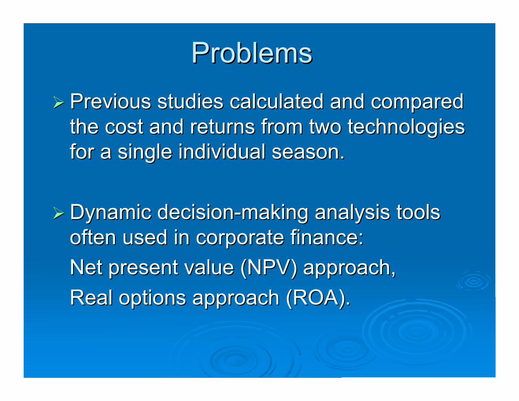
!! Previous studies calculated and comparedPrevious studies calculated and compared

the cost and returns from two technologiesthe cost and returns from two technologiesfor a single individual season.for a single individual season.

!! Dynamic decision-making analysis toolsDynamic decision-making analysis tools

often used in corporate finance:often used in corporate finance:

Net present value (NPV) approach,Net present value (NPV) approach,

Real options approach (ROA).Real options approach (ROA).

Objective of Our StudyObjective of Our Study

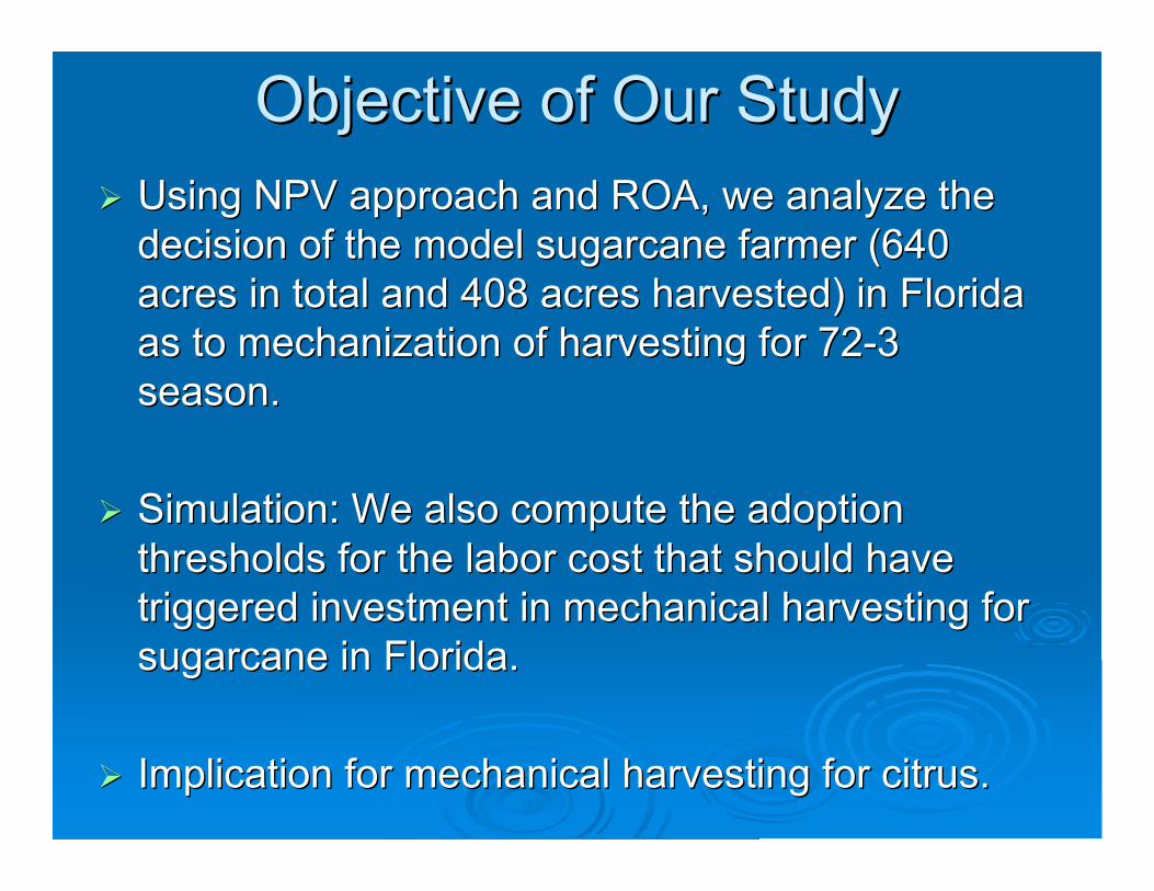
!! Using NPV approach and ROA, we analyze theUsing NPV approach and ROA, we analyze thedecision of the model sugarcane farmer (640decision of the model sugarcane farmer (640acres in total and 408 acres harvested) in Floridaacres in total and 408 acres harvested) in Floridaas to mechanization of harvesting for 72-3as to mechanization of harvesting for 72-3season.season.

!! Simulation: We also compute the adoptionSimulation: We also compute the adoptionthresholds for the labor cost that should havethresholds for the labor cost that should havetriggered investment in mechanical harvesting fortriggered investment in mechanical harvesting forsugarcane in Florida.sugarcane in Florida.

!! Implication for mechanical harvesting for citrus.Implication for mechanical harvesting for citrus.

NPV ApproachNPV Approach

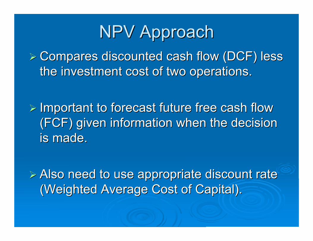
!! Compares discounted cash flow (DCF) lessCompares discounted cash flow (DCF) less

the investment cost of two operations.the investment cost of two operations.

!! Important to forecast future free cash flowImportant to forecast future free cash flow

(FCF) given information when the decision(FCF) given information when the decision

is made.is made.

!! Also need to use appropriate discount rateAlso need to use appropriate discount rate

(Weighted Average Cost of Capital).(Weighted Average Cost of Capital).

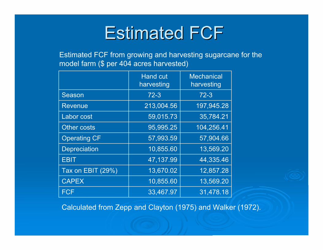
Estimated FCFEstimated FCFEstimated FCF from growing and harvesting sugarcane for themodel farm ($ per 404 acres harvested)

31,478.1833,467.97FCF

13,569.2010,855.60CAPEX

12,857.2813,670.02Tax on EBIT (29%)

44,335.4647,137.99EBIT

13,569.2010,855.60Depreciation

57,904.6657,993.59Operating CF

104,256.4195,995.25Other costs

35,784.2159,015.73Labor cost

197,945.28213,004.56Revenue

72-372-3Season

Mechanicalharvesting

Hand cutharvesting

Calculated from Zepp and Clayton (1975) and Walker (1972).

Forecasting Beyond 72-3 SeasonForecasting Beyond 72-3 Season

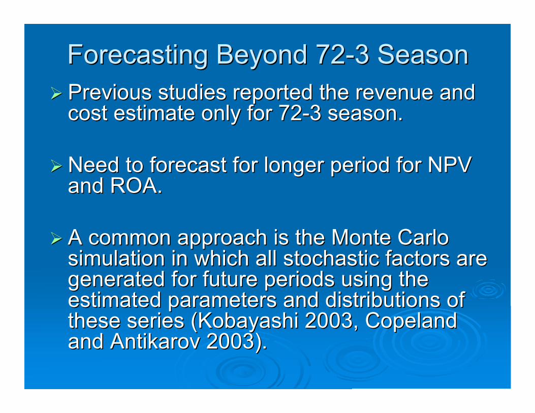
!! Previous studies reported the revenue andPrevious studies reported the revenue andcost estimate only for 72-3 season.cost estimate only for 72-3 season.

!! Need to forecast for longer period for NPVNeed to forecast for longer period for NPVand ROA.and ROA.

!! A common approach is the Monte CarloA common approach is the Monte Carlosimulation in which all stochastic factors aresimulation in which all stochastic factors aregenerated for future periods using thegenerated for future periods using theestimated parameters and distributions ofestimated parameters and distributions ofthese series (Kobayashi 2003, Copelandthese series (Kobayashi 2003, Copelandand and AntikarovAntikarov 2003). 2003).

Estimation of Stochastic ProcessEstimation of Stochastic Process

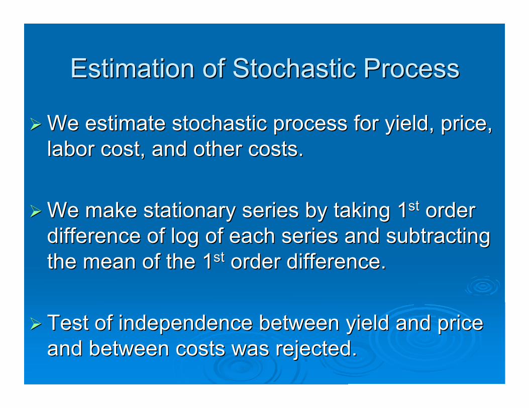
!! We estimate stochastic process for yield, price,We estimate stochastic process for yield, price,

labor cost, and other costs.labor cost, and other costs.

!! We make stationary series by taking 1We make stationary series by taking 1stst order order

difference of log of each series and subtractingdifference of log of each series and subtracting

the mean of the 1the mean of the 1stst order difference. order difference.

!! Test of independence between yield and priceTest of independence between yield and price

and between costs was rejected.and between costs was rejected.

Vector Autoregressive ModelVector Autoregressive Model

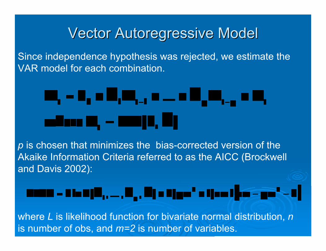
Since independence hypothesis was rejected, we estimate theVAR model for each combination.

p is chosen that minimizes the bias-corrected version of theAkaike Information Criteria referred to as the AICC (Brockwelland Davis 2002):

where L is likelihood function for bivariate normal distribution, nis number of obs, and m=2 is number of variables.

VAR ResultsVAR Results

!"

#$%

&+!"

#$%

&!"

#$%

&

'

'+

!"

#$%

&!"

#$%

& ''+!"

#$%

&=!

"

#$%

&

'

'

'

'

2

1

2,2

1,2

2,1

1,1

2

1

40.060.0

077.045.0

17.067.0

077.066.0

00.0

00.0

t

t

t

t

t

t

t

t

U

U

X

X

X

X

X

X

-74.55AICC and 042.00021.0

0021.00054.0,

0

0~ where

2

1=!

!"

#$$%

&'(

)*+

,

-

-'(

)*+

,'(

)*+

,WN

U

U

t

t

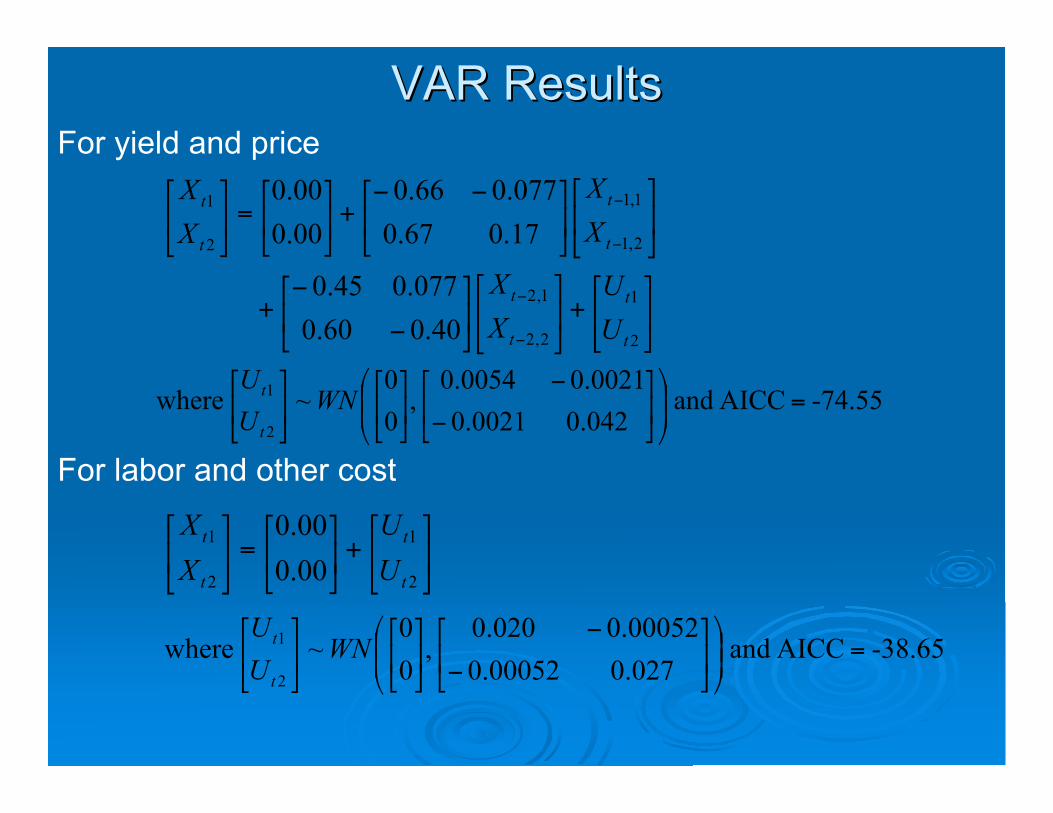
For yield and price

!"

#$%

&+!"

#$%

&=!

"

#$%

&

2

1

2

1

00.0

00.0

t

t

t

t

U

U

X

X

-38.65AICC and 027.000052.0

00052.0020.0,

0

0~ where

2

1=!

!"

#$$%

&'(

)*+

,

-

-'(

)*+

,'(

)*+

,WN

U

U

t

t

For labor and other cost

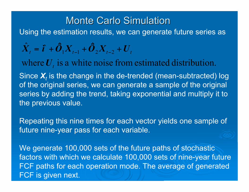
Monte Carlo SimulationMonte Carlo SimulationUsing the estimation results, we can generate future series as

on.distributi estimated from noise whitea is where

ˆˆˆˆ2211

t

tttt

U

UXÖXÖìX +++= !!

Since Xt is the change in the de-trended (mean-subtracted) logof the original series, we can generate a sample of the originalseries by adding the trend, taking exponential and multiply it tothe previous value.

Repeating this nine times for each vector yields one sample offuture nine-year pass for each variable.

We generate 100,000 sets of the future paths of stochasticfactors with which we calculate 100,000 sets of nine-year futureFCF paths for each operation mode. The average of generatedFCF is given next.

Monte Carlo Simulation (continued)Monte Carlo Simulation (continued)

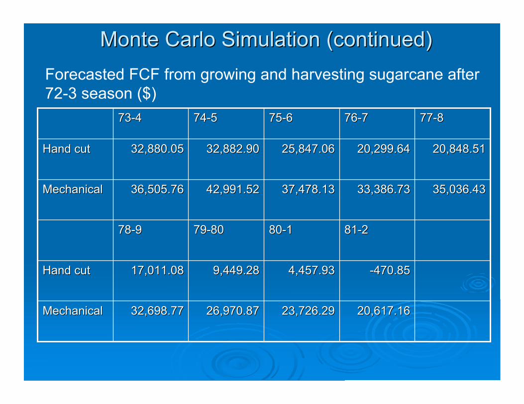
Forecasted FCF from growing and harvesting sugarcane after72-3 season ($)

20,617.1620,617.1623,726.2923,726.2926,970.8726,970.8732,698.7732,698.77MechanicalMechanical

-470.85-470.854,457.934,457.939,449.289,449.2817,011.0817,011.08Hand cutHand cut

81-281-280-180-179-8079-8078-978-9

35,036.4335,036.4333,386.7333,386.7337,478.1337,478.1342,991.5242,991.5236,505.7636,505.76MechanicalMechanical

20,848.5120,848.5120,299.6420,299.6425,847.0625,847.0632,882.9032,882.9032,880.0532,880.05Hand cutHand cut

77-877-876-776-775-675-674-574-573-473-4

Weighted Average Cost of CapitalWeighted Average Cost of Capital

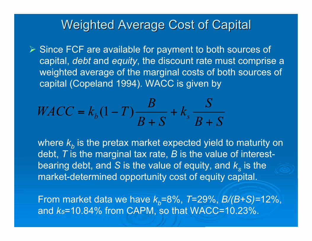
where kb is the pretax market expected yield to maturity ondebt, T is the marginal tax rate, B is the value of interest-bearing debt, and S is the value of equity, and ks is themarket-determined opportunity cost of equity capital.

From market data we have kb=8%, T=29%, B/(B+S)=12%,and ks=10.84% from CAPM, so that WACC=10.23%.

SB

Sk

SB

BTkWACC

sb

++

+!= )1(

! Since FCF are available for payment to both sources ofcapital, debt and equity, the discount rate must comprise aweighted average of the marginal costs of both sources ofcapital (Copeland 1994). WACC is given by

NPV CalculationNPV Calculation

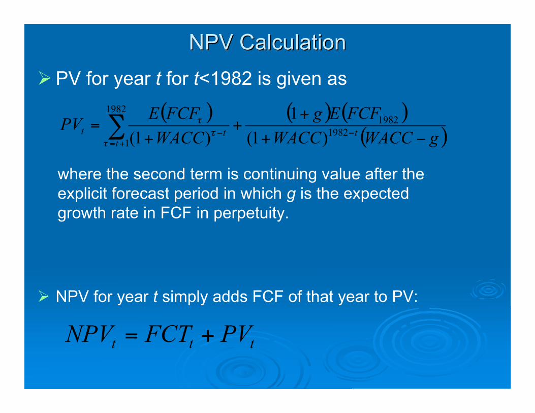
!PV for year t for t<1982 is given as

where the second term is continuing value after theexplicit forecast period in which g is the expectedgrowth rate in FCF in perpetuity.

( ) ( ) ( )( )gWACCWACC

FCFEg

WACC

FCFEPV

tt

tt!+

++

+=

!+=

!" 1982

19821982

1 )1(

1

)1(##

#

! NPV for year t simply adds FCF of that year to PV:

tttPVFCTNPV +=

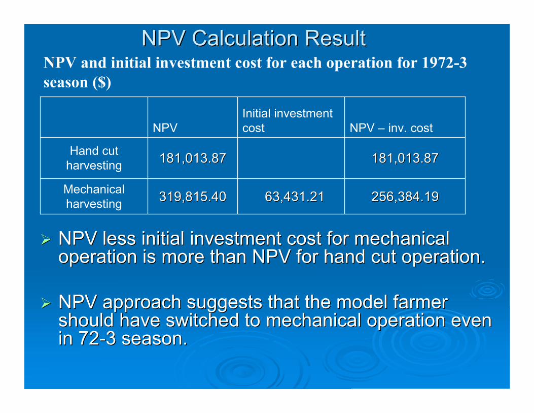
NPV Calculation ResultNPV Calculation Result

!! NPV less initial investment cost for mechanicalNPV less initial investment cost for mechanicaloperation is more than NPV for hand cut operation.operation is more than NPV for hand cut operation.

!! NPV approach suggests that the model farmerNPV approach suggests that the model farmershould have switched to mechanical operation evenshould have switched to mechanical operation evenin 72-3 season.in 72-3 season.

NPV and initial investment cost for each operation for 1972-3

season ($)

256,384.19 256,384.19 63,431.21 63,431.21319,815.40319,815.40Mechanicalharvesting

181,013.87181,013.87181,013.87181,013.87Hand cut

harvesting

NPV – inv. costInitial investmentcostNPV

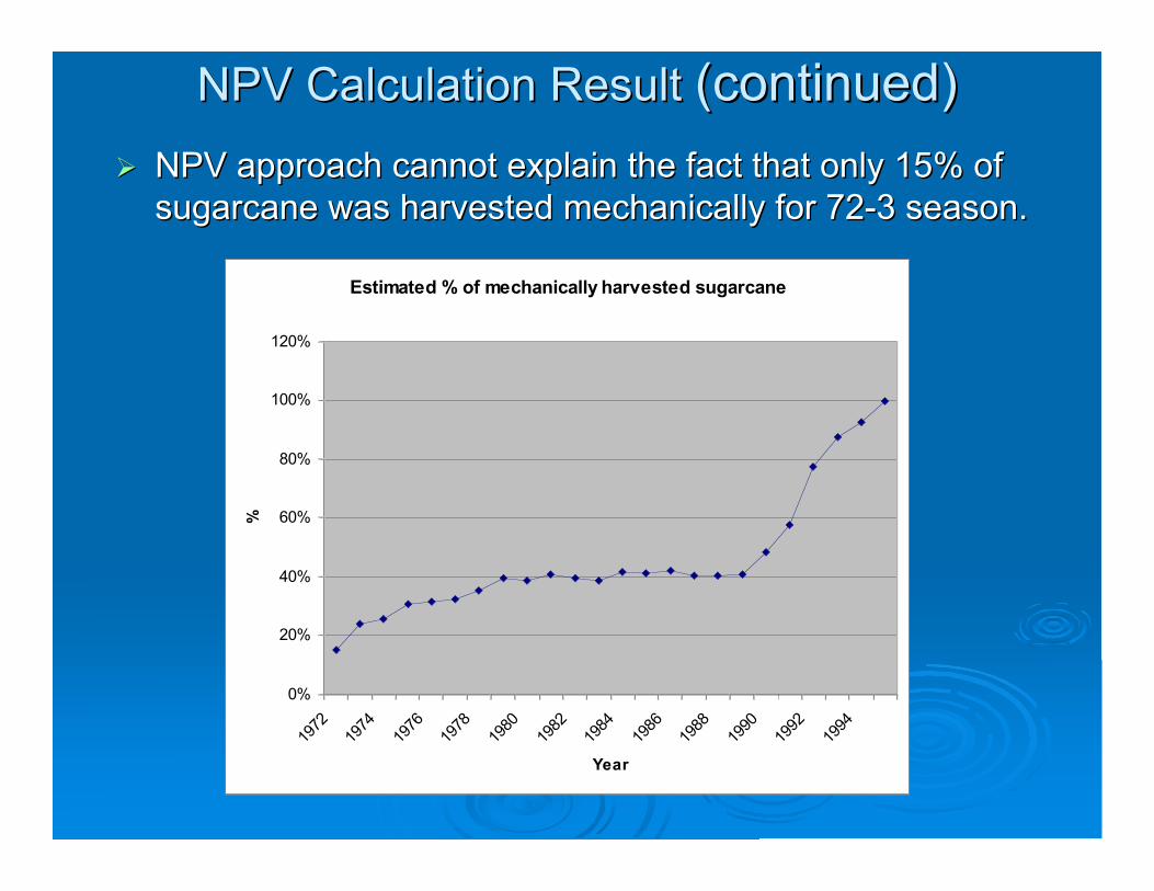
NPV Calculation Result NPV Calculation Result (continued)(continued)

Estimated % of mechanically harvested sugarcane

0%

20%

40%

60%

80%

100%

120%

1972

1974

1976

1978

1980

1982

1984

1986

1988

1990

1992

1994

Year

%

!! NPV approach cannot explain the fact that only 15% ofNPV approach cannot explain the fact that only 15% of

sugarcane was harvested mechanically for 72-3 season.sugarcane was harvested mechanically for 72-3 season.

Real Options ApproachReal Options Approach

!! ROA assumes that the producer has the option toROA assumes that the producer has the option toinvest or wait, called invest or wait, called ““investment flexibilityinvestment flexibility””..

!! However, once the producer makes an irreversibleHowever, once the producer makes an irreversibleinvestment, he exercises the option to invest andinvestment, he exercises the option to invest andgives up the option value of investment.gives up the option value of investment.

!! Hence the producer does not invest until the NPVHence the producer does not invest until the NPVless investment cost and option value of investmentless investment cost and option value of investmentopportunity is greater than the NPV for the currentopportunity is greater than the NPV for the currentoperation.operation.

Consolidated ApproachConsolidated Approach!! Our case study has four stochastic factors (yield,Our case study has four stochastic factors (yield,

price, labor cost and other costs).price, labor cost and other costs).

!! We use the consolidated approach (Copeland andWe use the consolidated approach (Copeland andAntikarovAntikarov 2003), which combines many stochastic 2003), which combines many stochasticfactors into one through the Monte Carlo simulation.factors into one through the Monte Carlo simulation.

!! The approach is based on the following theorem byThe approach is based on the following theorem bySamuelson (1973):Samuelson (1973):

““Regardless of the pattern of cash flows expected inRegardless of the pattern of cash flows expected inthe future, change in asset value is a random processthe future, change in asset value is a random processso that return is so that return is iidiid process, as long all the process, as long all theinformation about the expected future cash flows isinformation about the expected future cash flows isalready backed into the current value.already backed into the current value.””

Consolidated Approach (continued)Consolidated Approach (continued)

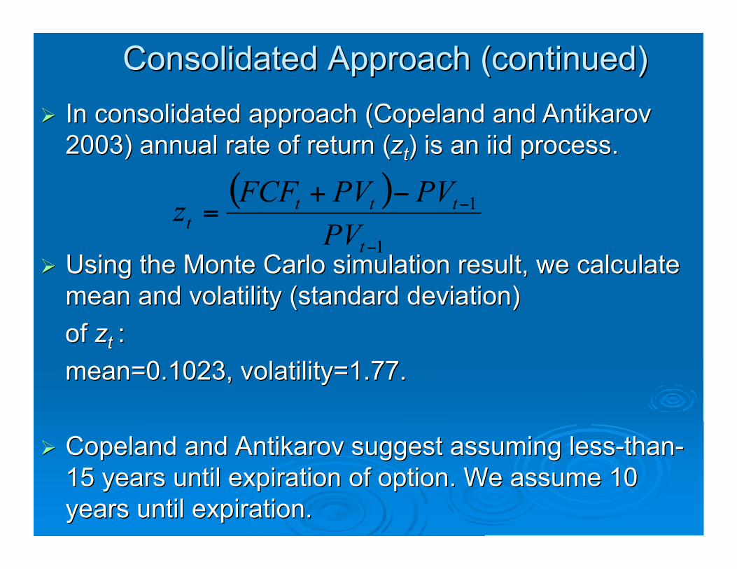
!! In consolidated approach (Copeland and In consolidated approach (Copeland and AntikarovAntikarov2003) annual rate of return (2003) annual rate of return (zztt) is an ) is an iidiid process. process.

( )

1

1

!

!!+=

t

ttt

t

PV

PVPVFCFz

!! Using the Monte Carlo simulation result, we calculateUsing the Monte Carlo simulation result, we calculatemean and volatility (standard deviation)mean and volatility (standard deviation)

of of zztt ::

mean=0.1023, volatility=1.77.mean=0.1023, volatility=1.77.

!! Copeland and Copeland and AntikarovAntikarov suggest assuming less-than- suggest assuming less-than-15 years until expiration of option. We assume 1015 years until expiration of option. We assume 10years until expiration.years until expiration.

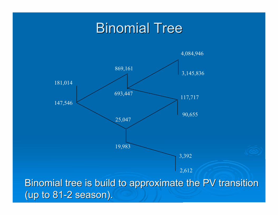
Binomial TreeBinomial Tree

Binomial tree is build to approximate the PV transitionBinomial tree is build to approximate the PV transition(up to 81-2 season).(up to 81-2 season).

181,014

19,983

147,546

25,047

869,161

693,447

4,084,946

3,145,836

117,717

90,655

3,392

2,612

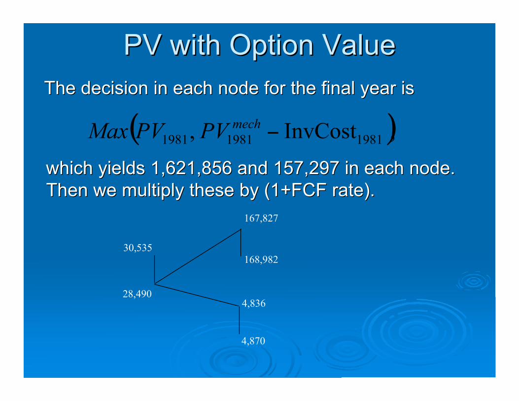
PV with Option ValuePV with Option Value

The decision in each node for the final year isThe decision in each node for the final year is

( ),InvCost ,198119811981

!mech

PVPVMax

which yields 1,621,856 and 157,297 in each node.which yields 1,621,856 and 157,297 in each node.Then we multiply these by (1+FCF rate).Then we multiply these by (1+FCF rate).

30,535

28,490

167,827

168,982

4,836

4,870

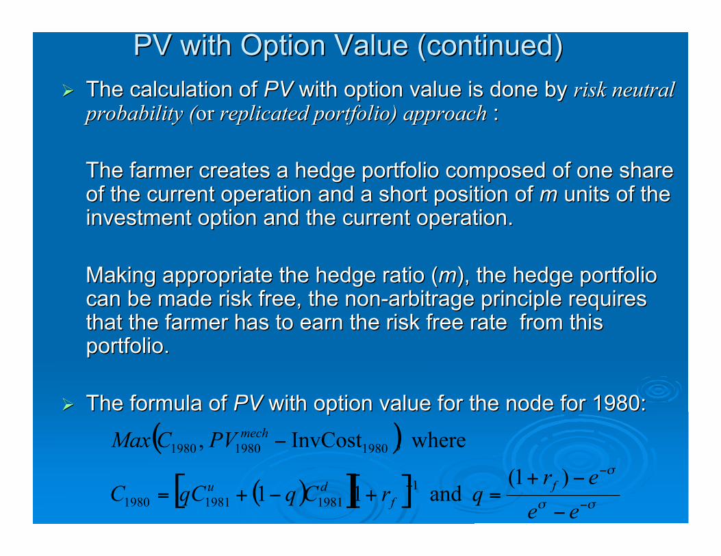
PV with Option Value (continued)PV with Option Value (continued)

!! The calculation of The calculation of PVPV with option value is done by with option value is done by risk neutralrisk neutralprobability (probability (oror replicated portfolio) approach replicated portfolio) approach ::

The farmer creates a hedge portfolio composed of one shareThe farmer creates a hedge portfolio composed of one shareof the current operation and a short position of of the current operation and a short position of mm units of the units of theinvestment option and the current operation.investment option and the current operation.

Making appropriate the hedge ratio (Making appropriate the hedge ratio (mm), the hedge portfolio), the hedge portfoliocan be made risk free, the non-arbitrage principle requirescan be made risk free, the non-arbitrage principle requiresthat the farmer has to earn the risk free rate from thisthat the farmer has to earn the risk free rate from thisportfolio.portfolio.

!! The formula of The formula of PVPV with option value for the node for 1980: with option value for the node for 1980:

( )

( )[ ][ ]!!

!

"

"

"

"

"+=+"+=

"

ee

erqrCqqCC

PVCMax

f

f

du

mech

)1( and 11

where,InvCost ,

1

198119811980

198019801980

PV with Option Value (continued)PV with Option Value (continued)

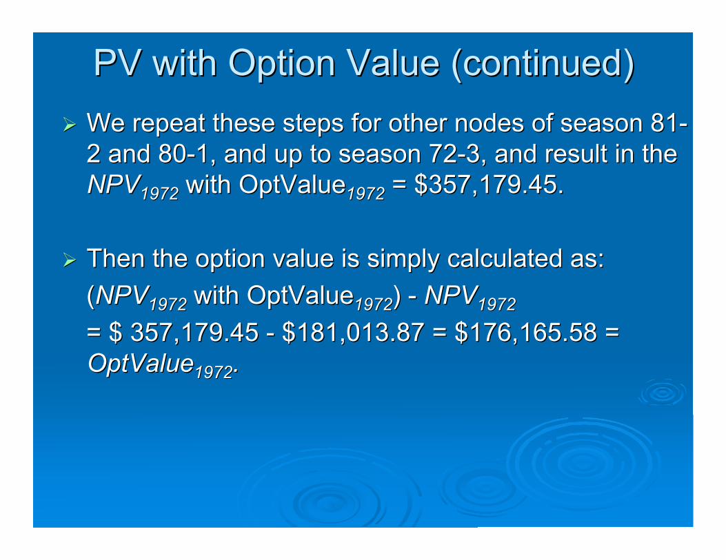
!! We repeat these steps for other nodes of season 81-We repeat these steps for other nodes of season 81-2 and 80-1, and up to season 72-3, and result in the2 and 80-1, and up to season 72-3, and result in theNPVNPV19721972 with OptValue with OptValue19721972 = $357,179.45. = $357,179.45.

!! Then the option value is simply calculated as:Then the option value is simply calculated as:

((NPVNPV19721972 with OptValue with OptValue19721972) - ) - NPVNPV19721972

= $ 357,179.45 - $181,013.87 = $176,165.58 == $ 357,179.45 - $181,013.87 = $176,165.58 =OptValueOptValue19721972..

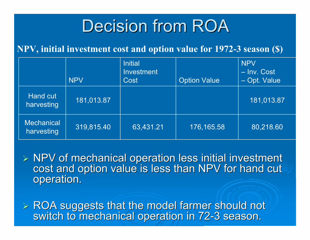
Decision from ROADecision from ROANPV, initial investment cost and option value for 1972-3 season ($)

176,165.58

Option Value

80,218.6063,431.21319,815.40Mechanicalharvesting

181,013.87181,013.87Hand cut

harvesting

NPV– Inv. Cost– Opt. Value

InitialInvestmentCostNPV

!! NPV of mechanical operation less initial investmentNPV of mechanical operation less initial investmentcost and option value is less than NPV for hand cutcost and option value is less than NPV for hand cutoperation.operation.

!! ROA suggests that the model farmer should notROA suggests that the model farmer should notswitch to mechanical operation in 72-3 season.switch to mechanical operation in 72-3 season.

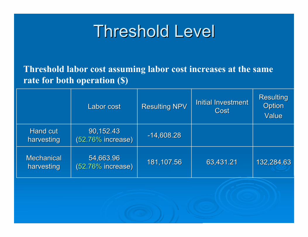
Threshold LevelThreshold Level

Threshold labor cost assuming labor cost increases at the same

rate for both operation ($)

63,431.2163,431.21

Initial InvestmentInitial Investment

CostCost

132,284.63132,284.63181,107.56181,107.5654,663.9654,663.96

((52.76%52.76% increase) increase)MechanicalMechanical

harvestingharvesting

-14,608.28-14,608.2890,152.4390,152.43

((52.76%52.76% increase) increase)Hand cutHand cut

harvestingharvesting

ResultingResulting

OptionOption

ValueValue

Resulting NPVResulting NPVLabor costLabor cost

ConclusionsConclusions

!!Previous studies found costPrevious studies found cost

advantage of mechanical harvestingadvantage of mechanical harvestingoperation over hand-cut as early asoperation over hand-cut as early as

72-3 season.72-3 season.

!! The NPV approach supports the views ofThe NPV approach supports the views ofprevious studies: NPV less initialprevious studies: NPV less initial

investment cost of mechanical operationinvestment cost of mechanical operation

($319,815) exceeds the NPV for hand cut($319,815) exceeds the NPV for hand cut

operation ($181,014).operation ($181,014).

Conclusions (continues)Conclusions (continues)!! Conclusion from ROA is opposite: Due to a highConclusion from ROA is opposite: Due to a high

volatility, the option value of holding investmentvolatility, the option value of holding investmentopportunity is high ($176,166) enough toopportunity is high ($176,166) enough tooverturn the conclusion of NPV.overturn the conclusion of NPV.

!! Threshold value analysis shows that it takesThreshold value analysis shows that it takesmore than more than 52%52% increase in labor cost for increase in labor cost forimmediate mechanization in 72-3 season.immediate mechanization in 72-3 season.

!! ROA explains better the historical fact that largeROA explains better the historical fact that largescale mechanization was delayed until mid/latescale mechanization was delayed until mid/late80s (only 80s (only 15%15% in 72-3 season). in 72-3 season).

Similar Situation of MechanicalSimilar Situation of MechanicalHarvesting for CitrusHarvesting for Citrus

!! Currently, mechanically harvesting Florida orangesCurrently, mechanically harvesting Florida orangesresults in about results in about 16%16% cost-savings ( cost-savings (25 cent per 9025 cent per 90pound box) pound box) relative to hand harvesting, under typicalrelative to hand harvesting, under typicalconditions (Roka 2008).conditions (Roka 2008).

!! Cost-savings suggest only two year payback period forCost-savings suggest only two year payback period forthe growerthe grower’’s investment in preparing the grove.s investment in preparing the grove.

!! Yet the adoption rate remains relatively low at aboutYet the adoption rate remains relatively low at aboutonly only 7.5%7.5% of the acreage. of the acreage.