UC Davis - CORE

UC DavisUC Davis Previously Published Works

TitleRefined knot invariants and Hilbert schemes

Permalinkhttps://escholarship.org/uc/item/6c02656f

JournalJournal des Mathematiques Pures et Appliquees, 104(3)

ISSN0021-7824

AuthorsGorsky, ENeguţ, A

Publication Date2015

DOI10.1016/j.matpur.2015.03.003 Peer reviewed

eScholarship.org Powered by the California Digital LibraryUniversity of California

brought to you by COREView metadata, citation and similar papers at core.ac.uk

provided by eScholarship - University of California

https://core.ac.uk/display/288432984?utm_source=pdf&utm_medium=banner&utm_campaign=pdf-decoration-v1

https://escholarship.org/uc/item/6c02656f

https://escholarship.org

http://www.cdlib.org/

arX

iv:1

304.

3328

v3 [

mat

h.R

T]

13 F

eb 2

015

REFINED KNOT INVARIANTS AND HILBERT SCHEMES

EUGENE GORSKY AND ANDREI NEGUT,

ABSTRACT. We consider the construction of refined Chern-Simons torusknot invariants byM. Aganagic and S. Shakirov from the DAHA viewpoint of I. Cherednik. We give a proofof Cherednik’s conjecture on the stabilization of superpolynomials, and then use the resultsof O. Schiffmann and E. Vasserot to relate knot invariants tothe Hilbert scheme of points onC2. Then we use the methods of the second author to compute theseinvariants explicitly inthe uncolored case. We also propose a conjecture relating these constructions to the rationalCherednik algebra, as in the work of the first author, A. Oblomkov, J. Rasmussen and V. Shende.Among the combinatorial consequences of this work is a statement of them

nshuffle conjecture.

1. INTRODUCTION

In [3], Aganagic and Shakirov defined refined invariants of the (m,n) torus knot by con-structing two matricesS andT that act on an appropriate quotient of the Fock space, andsatisfy the relations in the groupSL2(Z) (as in the work of Etingof and Kirillov). They conjec-tured that these invariants match the Poincare polynomials of Khovanov-Rozansky HOMFLYhomology ([47, 46]) of torus knots. The computation of Khovanov-Rozansky homology fortorus knots is a hard open problem in knot theory, and the Aganagic-Shakirov conjecture hasbeen verified in a few cases when this homology can be explicitly computed from the definition.

In [10], Cherednik reinterpreted the construction of [3] interms of the spherical double affineHecke algebraSH of typeA, by replacing theSL2(Z) action on the Fock space representa-tion by anSL2(Z) action on the DAHA. As such, he obtained a conjectural definition for thethree variable torus knot invariant known as thesuperpolynomial Pλ

n,m(u, q, t), defined forall partitionsλ and all pairs of coprime integersm,n. In Cherednik’s viewpoint, these super-polynomials arise as evaluations of certain elementsP λ

n,m in the DAHA. These elements arepolynomials in:

Pkn,km ∈ SH, ∀k ∈ Z,

by the same formula as the well-known Macdonald polynomialsPλ are polynomials in thepower sum functionspk, for all partitionsλ. The DAHA SH is bigraded in such a way thatPkn,km lies in bidegrees(kn, km), and the action ofSL2(Z) onSH is by automorphisms whichpermute the bidegrees of the elementsPkn,km. Cherednik constructs this action by a sequence ofelementary transformations, which are however rather difficult to describe by a closed formula.

Schiffmann and Vasserot ([60, 61]) give an alternate description of the DAHA by showingthat it is isomorphic to the elliptic Hall algebra. Under this automorphism,Pkn,km correspondto the standard generators of the elliptic Hall algebra described by Burban and Schiffmann in[8]. Moreover, Schiffmann and Vasserot show thatSH acts on theK−theory of the Hilbertscheme of points on the plane, and we will show that Cherednik’s superpolynomials can becomputed in this representation. We use this viewpoint to prove two conjectures announced byCherednik in [10] (let us remark that while the present paperwas being written, Cherednik alsoannounced independent proofs in [10, Section 2.4.1]). The occurrence of the Hilbert scheme isnot so surprising: Nakajima ([53]) already used it to compute the matricesS andT of Aganagicand Shakirov, although by using a different construction from ours.

1

http://arxiv.org/abs/1304.3328v3

2 EUGENE GORSKY AND ANDREI NEGUT,

An explicit description of the action ofPkn,km on theK−theory of the Hilbert scheme wasobtained in [54], where these operators were shown to be described by a certain geometriccorrespondence called the flag Hilbert scheme. We believe that a certain line bundle on thismoduli space is related to the unique finite-dimensional irreducible moduleLm

nof the rational

Cherednik algebra (see Conjecture 5.7 for a precise statement). A computational consequenceof our approach is the following formula for uncolored superpolynomials as a sum over stan-dard Young tableaux.

Theorem 1.1.The superpolynomialPn,m(u, q, t), defined as in[10], is given by:(1)

Pn,m(u, q, t) =∑

µ⊢n

γn

gµ

SYT∑

of shapeµ

∏ni=1 χ

Sm/n(i)

i (1− uχi)(qχi − t)(1− qχ2

tχ1

). . .(1− qχn

tχn−1

)∏

1≤i<j≤n

(χj − qχi)(tχj − χi)

(χj − χi)(tχj − qχi)

where the sum is over all standard Young tableaux of sizen, andχi denotes theq, t−1-weightof the box labeled byi in the tableau. The constants in the above relation are givenby:

(2) Sm/n(i) =

⌊im

n

⌋−

⌊(i− 1)m

n

⌋, γ =

(t− 1)(q − 1)

(q − t)

and:gµ =

∏

�∈λ

(1− qa(�)tl(�)+1)∏

�∈λ

(1− q−a(�)−1t−l(�))

The notions of arm-lengtha(�) and leg-lengthl(�) of a box in a Young diagram will berecalled in Figure 1.

We also give a prescription to compute general colored superpolynomialsPλn,m, for example

on a computer, although we do not yet have any “nice” formula.We use formulas such as (1)to explore many combinatorial consequences, such as to prove or formulate conjectures aboutq, t−Catalan numbers, parking functions and Tesler matrices in Section 6. The highlight isan m

nversion of the shuffle conjecture [40], where a certain combinatorial sum over parking

functions in anm × n rectangle obtained by Hikita [43] is connected with the operatorsPn,m

(see Conjecture 6.3 for all details). A sample of these results is a corollary of Conjecture 6.3,which appears to be new and interesting by itself:

Conjecture 1.2. The “superpolynomial”Pn,m(u, q, t) can be written as a following sum:

Pn,m(u, q, t) =∑

D

qδm,n−|D|t−h+(D)∏

P∈v(D)

(1− utβ(P ))

Here the summation is over all lattice pathsD contained below the main diagonal of anm×nl,P goes over all vertices ofD, δm,n = (m−1)(n−1)

2andh+(D) andβ(P ) are certain combinatorial

statistics (see Section 6.2 for details).

Form = n+1, the above identity was conjectured in [16] and proved in [37]. In the presentpaper, we prove this conjecture in the limitt = 1. For many values ofm andn, the aboveconjecture has been verified on a computer.

We also note that Conjecture 1.2 can be regarded as a refinement of [57, Conjectures 23,24].Indeed, in [57] the authors conjectured a relation between the Khovanov-Rozansky homologyof an algebraic knot and the homology of the Hilbert schemes of points on the correspondingplane curve singularity. For torus knots, these Hilbert schemes admit pavings by affine cells,and the homology can be computed combinatorially by counting these cells weighted with theirdimensions. It has been remarked in [57, Appendix A.3] that the corresponding combinatorial

REFINED KNOT INVARIANTS AND HILBERT SCHEMES 3

sum can be rewritten as a sum over lattice paths matching the combinatorial side of Conjecture1.2. Furthermore, it has been conjectured in [57, Conjectures 23,24] that the Poincare polyno-mial for the Khovanov-Rozansky homology of torus knots can be rewritten as an equivariantcharacter of the space of sections of a certain sheaf on the Hilbert scheme of points onC2, andthis sheaf was written explicitly form = kn± 1. For generalm, a construction of such a sheafor its class in the equivariantK-theory was not accessible by the methods of [57] (see [57, p.24] for the extensive computations).

In the present paper, we present a (conjectural) candidate for such a sheaf for allm co-prime withn, using the geometric realization ofPn,m(u, q, t). To summarize, one can say thatConjecture 1.2 would imply the agreement between the Aganagic-Shakirov and Oblomkov-Rasmussen-Shende conjectural descriptions of HOMFLY homology of torus knots, though,indeed, the relation between both of these descriptions to the actual definition of [47, 46] re-mains unknown.

Another conjecture relates the operatorPm,n to the finite-dimensional representationLmn

ofthe rational Cherednik algebra with parameterc = m

nequipped with a certain filtration defined

in [35]. Such a representation is naturally graded and carries an action of symmetric groupSn

preserving both the grading and the filtration.

Conjecture 1.3. The bigraded Frobenius character ofLmn

, equipped with the natural gradingand extra filtration (defined in [35]) equalsPm,n · 1.

This conjecture has bee mainly motivated by [35] whereLmn

has been related to the Hilbertschemes on the singular curve{xm = yn} and to the knot homology. Form = kn ± 1, theconjecture follows from the results of [27, 28].

The structure of this paper is the following: in Section 2, werecall the basics on symmet-ric functions, Macdonald polynomials, the double affine Hecke algebra, we state Cherednik’sconjectures 2.6 and 2.7, and recall how they relate to the original construction of Aganagicand Shakirov in Chern-Simons theory. In Section 3, we use thestabilization procedure ofSchiffmann-Vasserot to prove Cherednik’s conjectures by recasting his superpolynomials asmatrix coefficients. In Section 4, we discuss the Hilbert scheme and the flag Hilbert scheme,and show how the machinery of [54] gives new formulas for torus knot invariants. In Section 5,we discuss the connection between the Hilbert scheme and therational Cherednik algebra, andconjecture that a certain line bundle on the flag Hilbert scheme corresponds to the representa-tion Lm

nunder the Gordon-Stafford functor. Finally, in Section 6, we present certain aspects

from the combinatorics of symmetric functions which arise in connection to our work, stateseveral conjectures aboutq, t−Catalan numbers, parking functions and Tesler matrices, whichwe prove in several special cases.

ACKNOWLEDGMENTS

We are deeply grateful to Andrei Okounkov, who spurred this paper by explaining to usthe relation between the earlier results of the second author to the work of the first authoron knot invariants. He has helped us greatly with a lot of advice, and many interesting andeducating discussions. We are grateful to M. Aganagic, F. Bergeron, R. Bezrukavnikov, I.Cherednik, P. Etingof, A. Garsia, I. Gordon, J. Haglund, M. Haiman, A. Kirillov Jr., I. Losev,M. Mazin, H. Nakajima, N. Nekrasov, A. Oblomkov, J. Rasmussen, S. Shadrin, S. Shakirov,A. Smirnov, A. Sleptsov and V. Shende for their interest and many useful discussions. Specialthanks to Maxim Kazaryan for helping us with theMathematica code. The work of E.


G. was partially supported by the NSF grant DMS-1403560, RFBR grants RFBR-10-01-678,RFBR-13-01-00755 and the Simons foundation.

2. DAHA AND MACDONALD POLYNOMIALS

2.1. Symmetric functions. Consider formal parametersq andt, and let us define the followingring of constants and its field of fractions:

(3) K0 = C[q±1, t±1], K = C(q, t)

Among our basic objects of study will be the algebras of symmetric polynomials:

V = K[x1, x2, . . .]Sym, VN = K[x1, . . . , xN ]

Sym

In fact, the algebrasVN form a projective systemVN −→ VN−1, with the maps given by settingxN = 0, and the inverse limit of the system isV . An important system of generators for thesevector spaces consists of power-sum functionspk =

∑i x

ki , for which we have:

V = K[p1, p2, . . .], VN = K[p1, . . . , pN ]

A linear basis ofV is given by:

pλ = pλ1pλ2 . . . , as λ = (λ1 ≥ λ2 ≥ . . .)

go over all integer partitions. We have the scalar product〈·, ·〉 onV given by:

(4) 〈pλ, pµ〉 = δµλzλ ∀ λ, µ

wherez1n12n2 ... =∏

i≥1 inini!. Then another very important basis ofV is given by the Schur

functionssλ, which are orthogonal under the above scalar product and satisfy:

sλ = mλ +∑

µ<λ

cµλmµ for somecµλ ∈ Z

wheremλ = Sym(zλ11 zλ2

2 . . .)

are the monomial symmetric functions, and< denotes the dom-inance partial ordering on partitions:µ ≤ λ if µ1 + . . .+ µi ≤ λ1 + . . .+ λi for all i ≥ 1.

2.2. Macdonald polynomials. Another remarkable inner product onV was introduced byMacdonald [50]:

(5) 〈pλ, pµ〉q,t = δµλzλ∏

i

1− qλi

1− tλi∀ λ, µ

The Macdonald polynomialsPλ are defined by the property of being orthogonal with respectto 〈·, ·〉q,t and upper triangular in the basis of monomial symmetric functions:

Pλ = mλ +∑

µ<λ

dµλmµ for somedµλ ∈ K

The square norm ofPλ is given by:

〈Pλ, Pλ〉q,t =h′λ

hλ,

where:

hλ =∏

�∈λ

(1− qa(�)tl(�)+1), h′λ =

∏

�∈λ

(1− qa(�)+1tl(�))


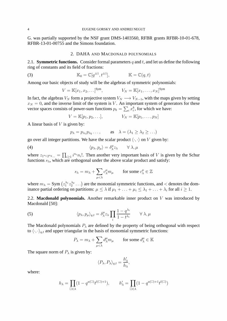
Here� goes over all the boxes in the Young diagram associated to thepartitionλ. The arm-lengtha(�) (respectively, the leg-lengthl(�)) is defined as the number of boxes above (re-spectively, to the right) of the box�. For illustration, see Figure 1.

a(�)a′(�)

l(�)

l′(�)

FIGURE 1. Arm, leg, co-arm and co-leg

There are various normalizations of Macdonald polynomials, and we will encounter theirintegral formJλ = hλPλ. We have:

(6) 〈Jλ, Jλ〉q,t = h2λ〈Pλ, Pλ〉q,t = hλh

′λ.

All these constructs make sense both inV (infinitely many variables) and inVN (finitely manyvariables), and they are compatible under the mapsV −→ VN . Let us now focus on the case offinitely many variables. Fix a positive integerN and let:

ρN = (N − 1, N − 2, . . . , 1, 0)

Consider the evaluation homomorphism:

(7) εN : VN −→ K, εN(f) = f(tρ) = f(tN−1, tN−2, . . . , 1)

A simple computation reveals that:

(8) εN(pk) =1− tkN

1− tk=

1− uk

1− tk,

where we capture theN-dependence in the new variableu = tN . Therefore, one can computeεN(f) for a general symmetric functionf by expanding it in terms of thepk and then using (8).

Theorem 2.1. ([50, eq. VI.6.17 and VI.8.8]) The following equations hold:

(9) εN(Pλ) =1

hλ

∏

�∈λ

(tl′(�) − uqa

′(�)) =⇒ εN(Jλ) =∏

�∈λ

(tl

′(�) − uqa′(�))

wherea′(�) (respectively,l′(�)) denote the co-arm and co-leg of� in λ (see Figure 1).

2.3. Double affine Hecke algebras.Following [14], we will define the double affine Heckealgebra (DAHA) of typeAN .

Definition 2.2. The algebraHN is defined overK by generatorsT±1i for i ∈ {1, . . . , N − 1},

andXj±1, Yj

±1 for j ∈ {1, . . . , N}, under the following relations:


(10)(Ti + t−1/2)(Ti − t1/2) = 0, TiTi+1Ti = Ti+1TiTi+1, [Ti, Tk] = 0 for |i− k| > 1

TiXiTi = Xi+1, Ti−1YiTi

−1 = Yi+1

[Ti, Xk] = 0, [Ti, Yk] = 0 for |i− k| > 1

[Xj , Xk] = 0, [Yj, Yk] = 0, Y1X1 . . .XN = qX1 . . .XNY1,X1−1Y2 = Y2X1

−1T1−2

The algebraHN contains the Hecke algebra generated byTi, and two copies of the affineHecke algebra generated by(Ti, Xj) and(Ti, Yj), respectively. The basic module ofHN is thepolynomial representation:

HN −→ End(C[X1, . . . , XN ]),

The elementXi acts as multiplication byxi, andTi acts by the Demazure-Lusztig operator:

Ti = t1/2si + (t1/2 − t−1/2)si − 1

xi/xi+1 − 1

wheresi = (i, i+1) are the simple reflections. Let us define the operators∂i onC[X1, . . . , XN ])by:

∂i(f) = f(x1, . . . , xi−1, qxi, xi+1, . . . xN ).

and introduce the operatorγ = sN−1 · · · s1∂1 Set:

Yi = tN−1

2 Ti · · ·TN−1γT−11 · · ·T−1

i−1.

Then the operatorsTi, Xj, Yj onVN satisfy the relations of the DAHA. A priori, these operatorsdo not necessarily send the subspace of symmetric polynomials VN to itself. However, it iswell-known that for any symmetric polynomialf , we have:

f(X1, . . . , Xn) : VN → VN , f(Y1, . . . , Yn) : VN → VN .

We will need the following result of Macdonald:

Proposition 2.3. ([50, eq. VI.3.4]) On the subspaceVN of symmetric polynomials, the operatorδ1 := Y1 + . . .+ YN can be rewritten as:

(11) δ1 =∑

i

Ai∂i, where Ai =∏

j 6=i

txi − xj

xi − xj

.

In fact, the operatorδ1 is diagonal in the basis of Macdonald polynomials ofVN , with eigen-values given by:

δ1 · Pλ(x) =

(∑

i

tN−iqλi

)Pλ(x).

This is part of an alternate definition of Macdonald polynomials as common eigenfunctions ofa collection of commuting differential operators, the firstof which isδ1. Generalizing this, thefollowing result is the main theorem of [12]:

Theorem 2.4([12]). Letf be a symmetric polynomial inN variables. The operator:

Lf := f(Y1, . . . , YN)

is diagonal in the basis of Macdonald polynomials inVN , with eigenvalues:

(12) Lf · Pλ(x) = f(tρN qλ)Pλ(x).


2.4. The SL2(Z) action. Letting e ∈ HN denote the complete idempotent, the sphericalDAHA is defined as the subalgebra:

SHN = e ·HN · e

There is an action ofSL2(Z) onHN that preserves the subalgebraSHN . To define it, let:

τ+ =

(1 10 1

), τ− =

(1 01 1

)

be the generators ofSL2(Z). Then Cherednik ([14], see also [61]) shows that:

(13) τ+(Xi) = Xi, τ+(Ti) = Ti, τ+(Yi) = YiXi(T−1i−1 · · ·T

−1i )(T−1

i · · ·T−1i−1)

τ−(Yi) = Yi, τ−(Ti) = Ti, τ−(Xi) = XiYi(Ti−1 · · ·Ti)(Ti · · ·Ti−1)

extend to automorphisms ofHN , and they respect the relations inSL2(Z). This action allowsone to construct certain interesting elements inHN . Start by defining:

P λ,N := Pλ(Y1, . . . , YN) ∈ SHN

For example,P (1),N = δ1 is the sum of theYi. For any pair of integers(n,m) with gcd(n,m) =1, let us choose any matrix of the form:

γn,m =

(x ny m

)∈ SL2(Z)

Definition 2.5. (andProposition, see [14], [61]) The elements:

P λ,Nn,m := γn,m(P

λ,N) ∈ SHN

do not depend on the choice ofγn,m.

The same construction can be done starting from the power-sum symmetric functions:

pNk := Y k1 + . . .+ Y k

N ∈ SHN .

Acting on them withγn,m gives rise to operators:

PNkn,km := γn,m(p

Nk ) ∈ SHN

As in the above Proposition, these do not depend on the particular choice ofγn,m. Since theMacdonald polynomialsP λ,N are polynomials in the power-sum functionspNk , then theP λ,N

n,m

are polynomials inPNkn,km. These can be easily calculated on a computer.

2.5. Cherednik’s conjectures. Following [10], we define theDAHA-superpolynomials:

Pλ,Nn,m(q, t) = εN(P

λ,Nn,m · 1) ∈ K, PN

kn,km(q, t) = εN(PNkn,km · 1) ∈ K

whereεN is the evaluation map of (7). Since the operatorsP λ,Nn,m can be expressed as sums of

products ofPNkn,km, we will see that the superpolynomialsPλ,N

n,m (q, t) can be expressed in termsof the matrix elements ofPN

kn,km. Therefore, we will mostly focus on the latter, and in Section4 we will show how to compute them. The following conjectureswere stated in [10]:

Conjecture 2.6(Stabilization). There exists a polynomialPλn,m(u, q, t) such that:

Pλ,Nn,m(q, t) = Pλ

n,m(u = tN , q, t)


Conjecture 2.7(Duality). Define the reduced superpolynomial by the equation:

Pλ,redn,m (u, q, t) =

Pλn,m(u, q, t)

Pλ1,0(u, q, t)

Then the polynomialsP for transposed diagrams are related by the equation:

q(1−n)|λ|Pλt,redn,m (u, q, t) = t(n−1)|λ|Pλ,red

n,m (u, t−1, q−1).

One of our main results is a proof of the above conjectures, tobe given in Subsections 3.4and 4.5.

2.6. Refined Chern-Simons theory. In this section we describe the approach of Aganagic andShakirov, which has its roots in Chern-Simons theory. A 3-dimensional topological quantumfield theory associates a numberZ(M) to every 3-manifold, a Hilbert spaceZ(N) to a closed2-manifoldN , and a vectorZ(M) ∈ Z(∂M) to a 3-manifoldM with boundary. All our3-manifolds may come with closed knots embedded in them.

We will be interested in invariants of torus knots inside thesphereS3. The sphere can besplit into two solid tori glued along the boundary, and the Hilbert spaceZ(T 2) associated totheir common boundary can be identified with a suitable quotient ofV . This quotient has abasis consisting of Macdonald polynomials labeled by Youngdiagrams inscribed in ak × Nrectangle. One can think of Macdonald polynomials as invariants of the meridian of the solidtorus colored by these diagrams. The spaceZ(T 2) is acted on by the mapping class group ofthe torus, namelySL2(Z), as constructed in [3].

Consider the(m,n) torus knot colored by a partitionλ inside a solid torus, linked with ameridian colored byµ. For such a link, a TQFT should produce a vectorvλn,m,µ in Z(T 2). Onedefines aknot operatorW λ

n,m by the formula:

W λn,m|Pµ〉 = vλn,m,µ.

In particular,W λn,m|1〉 is the vector inZ(T 2) associated to a solid torus with aλ-colored(m,n)

torus knot inside. The construction of [3] uses the equation:

(14) W λn,m = K−1W λ

1,0K,

whereW λ1,0 is the operator of multiplication byPλ andK is any element ofSL2(Z) taking

(1, 0) to (n,m), seen as an endomorphism ofZ(T 2). The action ofSL2(Z) was introduced byA. Kirillov Jr. in [48] and is given by the two matrices ([3, 19, 48]) written in the Macdonaldpolynomial basis1:

(15) Sµλ = Pλ(t

ρqµ)Pµ(tρ), T µ

λ = δµλq12

∑i λi(λi−1)t

∑i λi(i−1).

which correspond to the matrices:

σ =

(0 1−1 0

), τ =

(1 10 1

)∈ SL2(Z).

The refined Chern-Simons knot invariant is then defined as

(16) PCSn,m,λ(q, t) := 〈1|SW λ

n,m|1〉q,t.

The extraS-matrix in (16) is responsible for the gluing of two solid tori into S3. The equations(14)-(16) give a rigorous definition of the polynomialsPCS

n,mλ(q, t), which a priori depend on

1The operators in [3] differ from these by overall scalar factors, which are not important for us


the choice ofk andN . It is conjectured in [3] that for large enoughk andN the answer doesnot depend onk and itsN-dependence can be captured in a variableu = tN .

The approach of [10] is to identifyZ(T 2) with the finite-dimensional representation ofSHN .Such representations were classified in [64], and in typeAN they occur whenq is a root of unityof degreek+βN , andt = qβ. It is known ([13]) that the bilinear form〈·, ·〉q,t is nondegenerateonZ(T 2), which is a quotient of the polynomial representation by thekernel of this form. Thefollowing lemma shows the equivalence of the approaches of [3] and [10].

Lemma 2.8. In the representationZ(T 2), anyW ∈ SHN satisfies:

(17) SWS−1 = σ(W ).

whereσ acts on the DAHA as in Subsection 2.4.

Proof. By (12), we haveSµλ = εN(Pλ(Y ) · Pµ(x)). Consider the vector:

v = S(1) =∑

µ

εN(Pµ)Pµ

Then:S(Pλ) =

∑

µ

SµλPµ = Pλ(Y ) · v

hence we conclude that for any functionf ∈ VN , one hasS(f) = σ(f) · v. Therefore:

S(Wf) = σ(Wf) · v = σ(W )σ(f) · v = σ(W )S(f)

holds for anyW ∈ HN and anyf ∈ VN . �

Corollary 2.9. The definitions of the refined knot invariants in [3] and [10] are equivalent toeach other:

PCSn,m,λ(q, t) = Pλ,N

n,m (q, t).

Proof. Similarly to Lemma 2.8, one can show that the equationTWT−1 = τ(W ) holds foranyW ∈ SHN . Together with (17), this implies the equationKWK−1 = κ(W ), whereK isan arbitrary operator fromSL2(Z) andκ is the corresponding automorphism of the sphericalDAHA. In other words, the two actions ofSL2(Z) on the image ofSHN in the automorphismsof Z(T 2) agree with each other. Since bothP λ,N

1,0 andW λ,N1,0 are defined as multiplication

operators by the Macdonald polynomialPλ, one hasP λ,N1,0 = W λ,N

1,0 and

P λ,Nn,m = W λ,N

n,m

for all m, n andλ. It remains to notice that the covector〈1|S|·〉q,t coincides with the evaluationmapεN , hence

PCSn,mλ(q, t) = 〈1|SW λ

n,m|1〉q,t = εN(Wλn,m · 1) = εN(P

λn,m · 1) = Pλ,N

m,n (q, t).

�

3. STABILIZATION AND N -DEPENDENCE

Conjecture 2.6 involves theN-dependence of the expressionPλ,Nn,m = εN(P

λ,Nn,m · 1), and we

will understand this in three steps. First, we will recast the evaluationεN as a certain matrixcoefficient of the operatorP λ,N

n,m . Secondly, we will describe the behaviour of these operatorsasN → ∞ and show that they stabilize to an operatorP λ

n,m. Thirdly, we will discuss thebehaviour of the matrix coefficients asN → ∞.


3.1. Matrix Coefficients. Let us start from the polynomial representationSHN −→ End(VN).We will consider theevaluation vector:

(18) v(u) :=∑

λ

Jλ

hλh′λ

∏

�∈λ

(tl

′(�) − uqa′(�))∈ VN

In the above, the first sum goes over all partitions, and sov(u) rightfully takes values in acompletion ofVN . Then for anyf ∈ VN , we have:

εN(f) = 〈f,v(u)〉q,t

∣∣∣u=tN

Indeed, since the above relation is linear, it is enough to check it for f = Jλ, where it followsfrom (6) and (9). Then our knot invariants are given by the formula:

(19) Pλ,Nn,m = εN(P

λ,Nn,m · 1) = 〈v(u)|P λ,N

n,m |1〉q,t

∣∣∣u=tN

where〈·|∗|·〉q,t denotes matrix coefficients with respect to the Macdonald scalar product〈·, ·〉q,t.

3.2. Stabilization of operators. We will now letN vary. Recall that the spaces of symmetricpolynomialsVN form a projective system under the mapsηN : VN −→ VN−1 that setxN = 0,andV is the inverse limit if this system. Therefore, we have projection mapsη∞,N : V −→ VN .We will rescale our operators:

(20) PN

0,k = t−k(N−1)

(PN0,k −

tkN − 1

tk − 1

), P

N

kn,km = PNkn,km for n 6= 0

Proposition 3.1. (cf. [60, Prop. 1.4]) The following relation holds:

PN−1

kn,km ◦ ηN = ηN ◦ PN

kn,km

Therefore, there exist limiting operatorsPkn,km := limN→∞ PN

kn,km onV , such that:

PN

kn,km ◦ η∞,N = η∞,N ◦ Pkn,km

For a general partition, the operatorsP λ,Nn,m onVN are sums of products ofPN

kn,km, and thereforethere exist operatorsP λ

n,m onV which stabilize the operatorsP λ,Nn,m :

Pλ,N

n,m ◦ η∞,N = η∞,N ◦ P λn,m

All these new operatorsP λn,m andPkn,km lie in the algebraSH, defined in [60] as the stabiliza-

tion of the spherical DAHA’sSHN asN → ∞.

3.3. Commutation relations. The isomorphism betweenSH and the elliptic Hall algebra,established in [61] (see also [56]), allows one to present some explicit commutation relationsbetween the operatorsPn,m. These commutation relations were discovered by Burban andSchiffmann in [8]. It is sometimes convenient to represent the operatorPn,m by the vector(n,m) in the integer latticeZ2 (we assumen > 0). The action ofSL2(Z) on the algebraSH isthen just given by the linear action on this lattice.

Definition 3.2. ([56]) A triangle with verticesX = (0, 0), Y = (n2, m2) andZ = (n1 +n2, m1 +m2) is called quasi-empty ifm1n2 −m2n1 > 0 and there are no lattice points neitherinside the triagle, nor on at least one of the edgesXY, Y Z.


Let us define the constants:

(21) αn =(qn − 1)(t−n − 1)(q−ntn − 1)

n,

and the operatorsθkn,km (for coprimem,n) by the equation:

∞∑

n=0

znθkn,km = exp

(∞∑

n=1

αnznPkn,km

).

The elliptic Hall algebra is defined by the following commutation relations ([8]):

[Pn1,m1 , Pn2,m2 ] = 0,

if the vectors(n1, m1) and(n2, m2) are collinear, and:

(22) [Pn1,m1, Pn2,m2 ] =θn1+n2,m1+m2

α1,

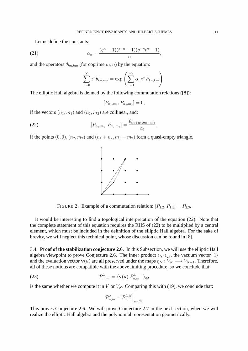
if the points(0, 0), (n2, m2) and(n1 + n2, m1 +m2) form a quasi-empty triangle.

• • • •

• • • •

• • • •

• • • •

FIGURE 2. Example of a commutation relation:[P1,2, P1,1] = P2,3.

It would be interesting to find a topological interpretationof the equation (22). Note thatthe complete statement of this equation requires the RHS of (22) to be multiplied by a centralelement, which must be included in the definition of the elliptic Hall algebra. For the sake ofbrevity, we will neglect this technical point, whose discussion can be found in [8].

3.4. Proof of the stabilization conjecture 2.6. In this Subsection, we will use the elliptic Hallalgebra viewpoint to prove Conjecture 2.6. The inner product 〈·, ·〉q,t, the vacuum vector|1〉and the evaluation vectorv(u) are all preserved under the mapsηN : VN −→ VN−1. Therefore,all of these notions are compatible with the above limiting procedure, so we conclude that:

(23) Pλn,m := 〈v(u)|P λ

n,m|1〉q,t

is the same whether we compute it inV or VN . Comparing this with (19), we conclude that:

Pλn,m = Pλ,N

n,m

∣∣∣u=tN

This proves Conjecture 2.6. We will prove Conjecture 2.7 in the next section, when we willrealize the elliptic Hall algebra and the polynomial representation geometrically.


4. THE HILBERT SCHEME OF POINTS

4.1. Basic Definitions. Let Hilbd = Hilbd(C2) denote the moduli space of colengthd ideal

sheavesI ⊂ OC2 . It is a smooth and quasi-projective variety of dimension2d. Pushing forwardthe universal quotient sheaf onHilbd×C2 gives rise to the rankd tautological vector bundle onHilbd:

T |I = Γ(C2,O/I)

The torusT = C∗ × C∗ acts onC2 by dilations, and therefore acts on sheaves onC2 bydirect image. This gives an action ofT on the moduli spacesHilbd. We can then consider theequivariantK−theory groupsK∗

T (Hilbd), all of which will be modules over:

K∗T (pt) = K0 = C[q±1, t±1]

whereq and t are a fixed basis of the characters ofT = C∗ × C

∗. As early as the work ofNakajima, it became apparent that one needs to study the direct sum of theseK−theory groupsover all degreesd. In other words, we will consider the vector space:

K =⊕

d≥0

K∗T (Hilbd)⊗K0 K

This vector space comes with the geometric pairing:

(24) (·, ·) : K ⊗K −→ K, (α, β) = π∗(α⊗ β)

whereπ : Hilbd −→ pt is the projection map. Feigin-Tsymbaliuk and Schiffmann-Vasserotindependently proved the following result:

Theorem 4.1. ([20], [60]) There exists a geometric action of the algebraSH on K, whichbecomes isomorphic to the polynomial representationV .

4.2. Torus fixed points. We have the following localization theorem in equivariantK−theory:

(25) K ∼=⊕

d≥0

K∗T (Hilb

Td )⊗K0 K

There are finitely many torus fixed points inHilbd, and they are all indexed by partitionsλ ⊢ d:

Iλ = (xλ1y0, xλ2y1, . . .) ⊂ C[x, y]

The skyscraper sheaves at these fixed points give a basisIλ = [Iλ] of the right hand side of(25), and therefore also of the vector spaceK. This basis is orthogonal with respect to thepairing (24):

(Iλ, Iµ) = δλ,µ · gλ

where:

(26) gλ := Λ•(T∨λ Hilbd) =

∏

�∈λ

(1− qa(�)t−l(�)−1)∏

�∈λ

(1− q−a(�)−1tl(�))

Theorem 4.2. (e.g. [42, 59]) Under the isomorphismK ∼= V of Theorem 4.1, the classesIλ ∈ K correspond to the modified Macdonald polynomials:

Hλ(q; t) = tn(λ)ϕ 11−1/t

[Jλ(q; t

−1)]∈ V

whereϕ 11−1/t

: V −→ V is the plethystic homomorphism defined bypk −→pk

1−1/tk, and:

(27) n(λ) =∑

�∈λ

l(�) =∑

�∈λ

l′(�)


The polynomialsHλ were introduced by Garsia and Haiman [24], and they are called modi-fied Macdonald polynomials. They behave nicely under transpose:

(28) Hλt(q; t) = Hλ(t; q).

Following [5], let us define the operator∇ onV by the formula:

(29) ∇Hλ = qn(λt)tn(λ)Hλ.

Under the isomorphismV ∼= K, ∇ corresponds to the operator of multiplication by the linebundleO(1), while the geometric inner product (24) corresponds to the following twist of theMacdonald inner product:

(30) (·, ·) = (−q)−d

⟨ϕ−1

11−1/t

(∇−1(·)

), ϕ−1

11−1/t

(·)

⟩

q,t−1

on Kd∼= Vd

4.3. Geometric operators. The most interesting elements ofSH to us arePkn,km, for allk 6= 0 andgcd(n,m) = 1. In the current geometric setting, we will study their conjugates:

(31) Pkn,km = ϕ 11−1/t

◦ Pkn,km(q; t−1) ◦ ϕ−1

11−1/t

Let us now describe how these operators act onK, and we will start with the simplest case,namelyn = 0. We define the polynomial:

(32) Λ(z) =

d∑

i=0

(−z)i[ΛiT ] ∈ K[z]

whereT is the tautological rankd vector bundle onHilbd. As was shown in [54], we have:

(33) exp

(∑

k≥0

αkP0,kzk

)· c =

Λ(qz

)Λ(tz

)Λ(

1zqt

)

Λ(

1zq

)Λ(

1zt

)Λ(qtz

) · c ∀c ∈ K

where the constantsαk are given by (21). In order to compute how eachP0,±k acts, we need toexpand the right hand side in powers ofz and take the appropriate coefficient. We will give amore computationally useful description ofP0,k in (36) below.

Forn > 0, we consider the flag Hilbert scheme:

Hilbd,d+kn = {I0 ⊃ I1 ⊃ . . . ⊃ Ikn} ⊂ Hilbd×Hilbd+1 × . . .× Hilbd+kn

where the inclusions are all required to be supported at the same point ofC2. This varietycomes with projection maps:

p− : Hilbd,d+kn −→ Hilbd, p+ : Hilbd,d+kn −→ Hilbd+kn

that forget all but the first/last ideal in the flag, and with tautological line bundlesL1, . . . ,Lkn

given by:

Li|I0⊃...⊃Ikn = Γ(C2, Ii−1/Ii)

As explained in [54], the flag Hilbert scheme is not simply theiteration ofkn individual Naka-jima correspondences. The reason for this is that the convolution product of Nakajima corre-spondences is not a complete intersection, and thus the intersection-theoretic composition is


a codimensionkn − 1 class on the schemeHilbd,d+kn. For this reason, the composition dif-fers significantly from the fundamental class ofHilbd,d+kn. In loc. cit., we have the followingdescription of the operatorsPkn,km acting onK:

(34) Pkn,km ·c =1

[k]·p+∗

[kn∏

i=1

[Lkn+1−i]⊗Sm/n(i) ⊗

(k−1∑

j=0

(qt)j · [Ln][L2n] · · · [Ljn]

[Ln+1][L2n+1] · · · [Ljn+1]

)· p−∗(c)

]

where we denote[k] = (qk−1)(tk−1)(q−1)(t−1)

andSm/n are the integral parts of (2). Note that the abovediffers by an overall normalizing constant from the operators of [54]. The above formula hasgeometric meaning, and in the next section we will make it more suitable for computations.

4.4. Matrix Coefficients. Let us compute the matrix coefficients(Iλ|Pkn,km|Iµ). Define:

(35) ω(x) =(x− 1)(x− qt)

(x− q)(x− t)

The easiest case for us isn = 0, sinceP0,k is multiplication with a givenK−theory class, andthus is diagonal in the basisIλ. More concretely, (33) yields:

exp

(∑

k≥0

αk(Iλ|P0,k|Iµ)zk

)= δµλ

∏

�∈λ

ω(

zχ(�)

)

ω(

χ(�)z

)

where given a box� = (i, j) in a Young diagram, itsweight is χ(�) = qi−1tj−1. Taking thelogarithm of the above gives us:

(36) (Iλ|P0,k|Iµ) = δµλ

((qt)k

(qk − 1)(tk − 1)+∑

�∈λ

χ(�)k

)

The matrix coefficients ofPkn,km for n > 0 are written in terms ofstandard Young tableaux(abbreviated SYT), so let us recall this notion. Given two Young diagramsρ1 ⊃ ρ2, a SYTbetween them is a way to index the boxes ofρ1\ρ2 with different numbers1, . . . , l such thatany two numbers on the same row or column decrease as we go to the right or up. We willoften write:

ρ1 = ρ2 +�1 + . . .+�l

if we want to point out that the box indexed byi is �i. Then [54] gives us the formula:

(Iµ|Pkn,km|Iλ) =γkn

[k]·gλgµ

SYT∑

µ=λ+�1+...+�kn

[k−1∑

j=0

(qt)jχn(k−1)+1χn(k−2)+1 · · ·χn(k−j)+1

χn(k−1)χn(k−2) · · ·χn(k−j)

]·

(37) ·

∏kni=1 χ

Sm/n(i)

i (qtχi − 1)(1− qtχ2

χ1

)· · ·(1− qt χkn

χkn−1

)∏

1≤i<j≤kn

ω−1

(χj

χi

) �∈λ∏

1≤i≤kn

ω−1

(χ(�)

χi

)

whereχi = χ(�i), γ = (q−1)(t−1)qt(qt−1)

andgλ are the equivariant constants of (26).

Remark4.3. Since the multiplication operators by power sumspn coincide with the operatorsPn,0, equation (37) can be used to compute their matrix elements in the modified Macdonaldbasis. Indeed, this computation will agree with the Pieri rules for Macdonald polynomials [50],so (37) can be considered as a generalization of Pieri rules.


4.5. Refined invariants via Hilbert schemes.Similarly to (31), we can define operatorsP λn,m

as conjugates toP λn,m underϕ 1

1−1/t. In particular, the operatorP λ

1,0 is conjugate byϕ 11−1/t

to the multiplication operator byPλ(q, t−1). Sinceϕ 1

1−1/tis a ring homomorphism,P λ

1,0 is a

multiplication operator by

ϕ 11−1/t

(Pλ(q, t−1)) =

t−n(λ)Hλ(q, t)

hλ(q, t−1).

and the action ofSL2(Z) implies:

(38) P λn,m :=

t−n(λ)

hλ(q, t−1)Hλ

[pk → Pkn,km

].

As was shown in (23), the super-polynomials are given by:

Pλn,m(u, q, t) =

⟨v(u)|P λ

n,m|1⟩q,t

, wherev(u) =∑

µ⊢n

Jµ

hµ(q; t)h′µ(q; t)

∏

�∈µ

(tl

′(�) − uqa′(�))

Under the isomorphism of Theorem 4.2, we can write the above as a matrix coefficient inK ∼= V :

(39) Pλn,m(u, q, t) =

(Λ(u)|P λ

n,m|1), whereΛ(u) =

∑

µ⊢n

Iµgµ

∏

�∈µ

(1− uqa

′(�)tl′(�))

and the change of variables is:

(40) Pλn,m(u, q, t) = (−q)−n|λ|Pλ

n,m(u, q, t−1)

By the equivariant localization formula, we see that theK−theory classΛ(u) defined aboveas a sum of fixed points coincides with the exterior class of (32). We have thus expressed oursuper-polynomials in terms of the geometric operators (34)on theK−theory of the Hilbertscheme.

Proof of Theorem 1.1.By (39), the uncolored DAHA – superpolynomial is given by:

Pn,m(u, q, t) = (Λ(u)|Pn,m|1) =∑

µ⊢n

(Iµ|Pn,m|1) ·

∏�∈µ(1− uχ(�))

gµ

We can use (37) to compute the above matrix coefficients, and we obtain:

(41) Pn,m(u, q, t) =

SYT∑

µ=�1+...+�n

γn

gµ·

∏ni=1 χ

Sm/n(i)

i (1− uχi)(qtχi − 1)(1− qtχ2

χ1

)· · ·(1− qt χn

χn−1

)∏

1≤i<j≤n

ω−1

(χj

χi

)

Changingt → t−1 gives us formula (1). �

As for the colored knot invariantPλn,m , it is also a particular matrix coefficient of the operator

P λn,m:

Pλn,m(u, q, t) = (Λ(u)|P λ

n,m|1) =∑

µ⊢n|λ|

(Iµ|Pλn,m|1) ·

∏�∈µ(1− uχ(�))

gµ


By (38), the operatorP λn,m expands in the operatorsPnk,mk given by the same formula as

modified Macdonald polynomials expand in the power-sum functionspk. For computationalpurposes, the task then becomes to compute expressions of the form:

∑

µ⊢n(k1+...+kt)

(Iµ|Pnk1,mk1 · · · Pnkt,mkt|1) ·

∏�∈µ(1− uχ(�))

gµ

for anyk1, . . . , kt. These can be computed by iterating (37) and the result will be a sum overstandard Young tableaux. The summand will be in general morecomplicated than (41), but itcan be taken care of by a computer. While we do not yet have a “nice” formula suitable forwriting down in a theoretical paper, we may use the geometricviewpoint to prove Cherednik’ssecond conjecture:

Proof of Conjecture 2.7.In terms of the modified superpolynomialsP, the desired identity be-comes:

Pλt,redn,m (u, q, t) = Pλ,red

n,m (u, t, q), wherePλ,redn,m (u, q, t) := (−q)−(n−1)|λ|Pλ,red

n,m (u, q, t−1).

Recall that

Pλ1,0(u, q, t) =

1

hλ(q, t)

∏

�∈λ

(tl′(�) − uqa

′(�)),

so

Pλ1,0(u, q, t) =

t−n(λ)

hλ(q, t−1)

∏

�∈λ

(1− uqa′(�)tl

′(�)),

hence


Pλn,m(u, q, t)

Pλ1,0(u, q, t)

=hλ(q, t

−1)(Λ(u)|P λn,m|1)

t−n(λ)∏

�∈λ(1− uqa′(�)tl′(�)).

Therefore by (38) we get


(Λ(u)|Hλ(q, t)

[pk → Pkm,kn

]|1)

∏�∈λ(1− uqa′(�)tl′(�))

.

By (28) Hλ(q, t) = Hλt(t, q), and by (37) the matrix coefficients ofPkm,kn are invariant underthe switchingq ↔ t and the transposition of the axis, as well asΛ(u). �

4.6. Constant term formulas. Formula (41) can be repackaged as a contour integral. We maywrite:

Pn,m(u, q, t) = (Λ(u)|Pn,m|1) = (1|P−n,m|Λ(u))

whereP−n,m is the adjoint ofPn,m. Formula (4.12) of [54] gives us the following integralformula for this expression:

(42) Pn,m(u, q, t) =

∫ ∏ni=1 z

Sm/n(i)

i · 1−uzizi−1(

1− qtz2z1

)· · ·(1− qt zn

zn−1

)∏

1≤i<j≤n

ω

(zizj

)dz12πiz1

· · ·dzn2πizn

where the contours of the variableszi surround 1, withz1 being the outermost andzn being theinnermost (we takeq, t very close to 1). We can move the contours so that they surround 0 and∞, and then the integral comes down to the following residue computation:

Pn,m(u, q, t) = (Reszn=0 − Reszn=∞) · · · (Resz1=0 − Resz1=∞)


(43)1

z1 · · · zn·

∏ni=1 z

Sm/n(i)

i · 1−uzizi−1(

1− qtz2z1

)· · ·(1− qt zn

zn−1

)∏

1≤i<j≤n

ω

(zizj

)

We will compute the above residue in section 6.5, which will give another combinatorial wayto computePn,m.

4.7. Let us say a few words about the viewpoint of Nakajima in [53], which relates knotinvariants to the following map:

Ψd : V −→ Kd, Ψd(f) = f(W∨)

whereW is the universal bundle onHilbd. As aK−theory class (and this will be sufficient forthe purposes of the present paper), it is given by[W] = 1 − (1 − q)(1 − t)[T ]. We may takethe direct product of the above maps over alld and define:

(44) Ψ : V −→ K, Ψ =

∞∏

d=0

Ψd

The mapΨ defined above takes values in a certain completion ofK, since we consider thedirect product. Via equivariant localization, we see that:

(45) Ψ(f) =∑

λ

Iλgλ

· f

(1− (1− q−1)(1− t−1)

∑

�∈λ

χ(�)−1

)

The right hand side of (45) uses plethystic notation of symmetric functions, which is describedin [53]. In loc. cit., Nakajima uses the map (44) to study knot invariants, essentially by usingthe viewpoint given by the left hand side of relation (17) where theS-matrix is realized as anoperator onVN . Our viewpoint, outlined in the previous sections, is to compute the same knotinvariants by using the right hand side of (17) and interpretS as an automorphism of the algebraSH. The two perspectives produce significantly different formulas.

5. REPRESENTATIONS OF THE RATIONALCHEREDNIK ALGEBRA

5.1. The rational Cherednik algebra. Rational Cherednik algebras were introduced in [17]as degenerations of the DAHA.

Definition 5.1. The rational Cherednik algebra of typeAn−1 with parameterc is:

Hc = C[h]⊗ C[h∗]⋊ C[Sn],

whereh is the Cartan subalgebra ofsln, and the commutation relations between the variousgenerators are:

[x, x′] = 0, [y, y′] = 0, gxg−1 = g(x), gyg−1 = g(y),

[x, y] = (x, y)− c∑

s∈S

(αs, x)(α∗s, y)s,

for anyx ∈ h∗, y ∈ h, g ∈ Sn. HereS denotes the set of all reflections inSn andαs is theequation of the reflecting hyperplane ofs ∈ S.


The polynomial representation also makes sense for rational Cherednik algebras, and itsrepresentation space isMc(n) = C[h]. The symmetric group acts naturally,h acts by multipli-cation operators and elements ofh∗ act by Dunkl operators:

Dy = ∂y − c∑

s∈S

(αs, y)

αs(1− s)

As a generalization of this construction, one can consider the standard module:

Mc(λ) = τλ ⊗ C[h],

whereλ is any partition andτλ is the corresponding irreducible representation ofSn. It iswell-known thatMc(λ) has a unique simple quotientLc(λ).

5.2. Finite-dimensional representations. It turns out that the representation theory of therational Cherednik algebra depends crucially on the parameter c. For example, we have thefollowing classification of finite-dimensional representations.

Theorem 5.2([4]). The algebraHc only has finite-dimensional representations ifc = mn

forsomegcd(m,n) = 1, in which case it has a unique irreducible representation

Lmn= Lm

n(n).

Furthermore (ifm > 0), one has

dimLmn= mn−1, dim(Lm

n)Sn =

(m+ n− 1)!

m!n!.

The representationLmn

is canonically graded and carries a grading-preserving action of Sn.In particular, it is a representation ofSn, so we can define its Frobenius character:

chLmn=

1

n!

∑

σ∈Sn

TrLmn(σ)pk11 . . . pkrr

wherepi are power sums, andki is the number of cycles of lengthi in the permutationσ. TheFrobenius character makes sense for any representation ofSn, and in particular the Frobeniuscharacter of the irreducibleτλ equals the Schur polynomialsλ.

Theorem 5.3([4]). The graded Frobenius character ofLmn

equals

chq Lmn=

q−(m−1)(n−1)

2

[m]qφ[m](hn),

where[m]q =1−qm

1−qandφ[m] : Λ → Λ is the homomorphism defined byφ[m](pk) = pk

1−qkm

1−qk.

For m = n + 1, Gordon observed a close relation between the representation Ln+1n

andHaiman’s work. Gordon constructs a certain filtration onLn+1

nand proves the following result.

Theorem 5.4([26]). The bigraded Frobenius character ofgrLn+1n

is given by the formula

chq,t grLn+1n

= ∇en.

In [35], Gordon’s filtration was generalized to all finite-dimensional representationsLmn

and it was conjectured that the bigraded charactergrLmn

is tightly related to the Khovanov-Rozansky homology of the(m,n) torus knot. In light of the conjectures of [3], we formulatethe following:


Conjecture 5.5. The bigraded Frobenius character ofgrLmn

is given by:

chq,t grLmn= Pn,m · 1

wherePn,m are the transformed DAHA elements of Subsection 4.3.

Whenm = n+1, the conjecture follows from Theorem 5.4 and Corollary 6.5 below. Conjec-ture 5.5 is also supported by numerical computations, and itis compatible with some structuralproperties. For example, the symmetry between theq andt gradings of the character has beenproven in [35], and this symmetry is manifest in the operators Pn,m. Moreover, Conjecture5.5 was proved inloc. cit. at t = q−1, by showing that the knot invariant equals the singlygraded Frobenius character, see also Section 6.7 for details. It was also observed by Gordonand Stafford that:

chq,t grLm+nn

= ∇ chq,t grLmn,

where∇ is the operator of (29). This matches with the equality:

(46) Pn,n+m = ∇Pn,m∇−1

which follows easily from the definition ofPn,m in Subsection 4.3.

Remark5.6. The above only deals with the uncolored case, since the representation-theoreticinterpretation of colored refined knot invariants has yet tobe developed. It is proved in [18] thatat t = q−1 the unrefinedλ-colored invariant of the(m,n) torus knot is given by the characterof the infinite-dimensional irreducible representationLm

n(nλ). It would be interesting to define

a filtration onLmn(nλ) that matches their character with refined invariants.

5.3. The Gordon-Stafford construction. Conjecture 5.5 is part of a correspondence betweenrepresentations of the rational Cherednik algebra and coherent sheaves on Hilbert schemes,which we will now discuss. Kashiwara and Rouquier ([44]) have constructed a quantization ofthe Hilbert scheme depending on the parameterc, such that the category of coherent sheavesover this quantization is equivalent to the category of representations ofHc. In characteristicp,the analogous construction has been carried out by Bezrukavnikov-Finkelberg-Ginzburg ([7]).We will only be concerned with characteristic 0, in which case the initial result of Gordon andStafford ([27]) claims the existence of a map:

(47) DbRep(Hc) −→ DbCoh(Hilbn)

for all c. The category on the left consists of filtered representations (see [27] for the exactdefinition) of the rational Cherednik algebra. One may ask about the image of the uniqueirreducible finite-dimensional representationLm

nunder the above assignemnt. During our dis-

cussions with Andrei Okounkov, the following conjecture was proposed:

Conjecture 5.7. Under the Gordon-Stafford map (47),Lmn

is sent to:

(48) Fmn:= p∗

(L

Sm/n(1)n ⊗ . . .⊗L

Sm/n(n)

1

)

wherep : Hilb0,n −→ Hilbn is the projection map from the flag Hilbert scheme to the Hilbertscheme (see Subsection 4.3 for the notations), andL1, . . . ,Ln are the tautological line bundles.

The flag Hilbert scheme together with the projectionp should be understood in the DG sense,see [54] for details. In fact, the above conjecture is a particular case of a far-reaching conjecturalframework of Bezrukavnikov–Okounkov, concerning filtrations on the derived category of theHilbert scheme.


To support Conjecture 5.7, note that the functor (47) matches the bigraded character of repre-sentations with the biequivariantK−theory classes of coherent sheaves. Therefore, Conjecture5.7 implies that:

chq,t grLmn=[p∗

(L

Sm/n(1)n ⊗ · · · ⊗ L

Sm/n(n)

1

)]

Comparing with (34), we see that the object in the right hand side is simplyPn,m · 1 ∈ K.Therefore, Conjecture 5.7 implies Conjecture 5.5.

5.4. Affine Springer fibres. Yet another geometric realization ofLmn

is provided by the affineSpringer fibres in the affine flag variety. Let us recall that the affine GrassmannianGrn of typeAn−1 can be defined as the moduli space of subspacesV ⊂ C((t)) satisfyingtnV ⊂ V anda certain normalization condition. Similarly, the affine flag varietyFln can be defined as themoduli space of flags of subspaces inC((t)) of the formV1 ⊃ V2 ⊃ . . . ⊃ Vn ⊃ Vn+1 = tnV1

such thatdimVi/Vi+1 = 1.Recall that an affine permutation (of typeAn−1) is a bijectionω : Z → Z such thatω(x+n) =

ω(x) + n for all x and∑n

i=1 ω(i) =n(n+1)

2. It is well known thatFln is stratified by the affine

Schubert cellsΣω labelled by the affine permutations. Thehomogeneous affine Springer fiber:

Σmn⊂ Fln (resp.ΣGr

mn⊂ Grn)

is defined as as set of flags (resp. subspaces) invariant undermultiplication bytm, where, asabove, we assume thatgcd(m,n) = 1. It is known to be a finite-dimensional projective variety[29, 45, 49] and the total dimension of the homology equals ([43, 49]):

dimH∗(Σmn) = mn−1, dimH∗(ΣGr

mn) =

(m+ n− 1)!

m!n!.

The similarity between this equation and Theorem 5.2 suggests a relation betweenLmn

and thehomology ofΣm

n. Indeed, in [58, 64] the authors constructed geometric actions of the DAHA

and trigonometric / rational Cherednik algebras on the spaceH∗(Σmn) equipped with certain fil-

trations. In all these constructions, the spherical parts of the corresponding representations canbe naturally identified withH∗(ΣGr

mn), also equipped with certain filtrations. It is important to

mention that the homological grading onH∗(Σmn) does notmatch the representation-theoretic

grading onLmn

. On the other hand, thebigradedcharacter ofgrH∗(Σmn) is expected to match

the bigraded character ofgrLmn

after some regrading, when one takes into account both thegeometric filtration on the homology and the generalized Gordon filtration onLm

n(see [35] for

the precise conjecture).In the next section we give an explicit combinatorial counterpart of this conjecture (Con-

jecture 6.3), which can be explicitly verified on a computer.By Conjecture 5.5, the bigradedcharacter ofgrLm

nis given byPn,m · 1 and hence can be computed combinatorially using (37).

On the other hand, one can try to compute the bigraded character of grH∗(Σmn) using some

natural basis in the homology, which is expected to be compatible with the geometric filtration.

Definition 5.8. ([34]) We call an affine permutationω m–stable, ifω(x+m) > ω(x) for all x.

Theorem 5.9. ([34]) The intersection of an affine Schubert cell with the affine Springer fiberΣm

nis either empty or isomorphic to an affine space. The nonemptyintersections correspond to

them-stable affine permutationsω, and the dimension of the corresponding cell inΣmn

equals:

dimΣω ∩ Σmn= | {(i, j)|ω(i) < ω(j), 0 < i− j < m, 1 ≤ j ≤ n} |.


In the homology ofΣmn

one then have a combinatorial basis corresponding to these cells,with the homological gradings given by the above equation. In [34] them-stable affine per-mutations has been identified by an explicit bijection with another combinatorial object, theso-calledm/n-parking functions, see Section 6.3. The dimension of a cellis translated to acertain combinatorial statistics dinv on parking functions, which has been obtained earlier byHikita in [43]. We also conjecture that the geometric filtration on the homology is compatiblewith the basis of cells, and admits an easy combinatorial description as the “area” of the corre-sponding parking function. Modulo this conjecture, one canshow that the bigraded characterof grH∗(Σm

n) coincides with the combinatorial expression (51).

One can similarly describe the cell decomposition ofΣGrmn

, which turns out to coincide withthe compactified Jacobian of the plane curve singularity{xm = yn}. The affine Schubert cellsin Grn cut out affine cells inΣGr

mn

, which can be labeled either by them–stable permutationswith additional restrictions ([34]) or by the Dyck paths in them × n rectangle ([32, 33]). Thedimension of such a cell can be rewritten as(m−1)(n−1)

2− h+(D), whereh+(D) is an explicit

combinatorial statistic on the corresponding Dyck pathD (see Section 6.2).

6. COMBINATORIAL CONSEQUENCES

6.1. In this section we focus on the combinatorial structureof uncolored refined knot polyno-mials. By (41), we have forgcd(n,m) = 1:

(49) Pn,m · 1 =∑

λ⊢n

cn,m(λ)Hλ

gλ,

wherecn,m(λ) is the sum of termscn,m(T ) over all standard Young tableauxT of shapeλ:

(50) cn,m(T ) = γn

∏ni=1 χ

Sm/n(i)

i (qtχi − 1)∏n−1

i=1

(1− qtχi+1

χi

)∏

1≤i<j≤n

ω−1

(χj

χi

)

Recall thatχi denotes the weight of boxi in the standard Young tableauT and the constantsSm/n(i) are defined by (2). Some of the coefficientscn,m(λ) have appeared in various sources:for m = 1 they are remarkably simple and were computed first in [23] andlater rediscovered in[57, 62]. For generalm and smalln some of these coefficients were computed in [57, Section5.3], [15] and [62]. Although the individual termscn,m(T ) have a nice factorized form, theirsumscn,m(λ) look less attractive, for example:

c7,2(4, 3) = (1− q)2(1− t)2(1− t2)(1− t3)(qt− 1)

(q3t3 + q3t2− q3 + q2t5 +2q2t4 + q2t3 − q2t+ qt6 + qt5 − qt4 − 2qt3− qt2 + t7 − t5 − t4 − t3)

For hook shapes of sizen, the coefficientscn,m(k, 1, . . . , 1) are equal to a product of linearfactors times a sum ofn terms. Explicitly, the following formula was computed in [55] usingshuffle algebra machinery:

cn,m(k, 1, . . . , 1) =(1− q)(1− t)

qntn

k−1∏

i=1

(1− qi)

n−k∏

i=1

(1− ti)

(n−1∑

i=0

q∑k−1

j=0⌊mj+i

n ⌋t∑n−k

j=1 ⌈mj−i

n ⌉

)

for all coprimem andn, and all1 ≤ k ≤ n. For smallk, this agrees with the computationsin [57, Section 5.3]. Further, we give a combinatorial interpretation of uncolored refined knotinvariants, generalizing the so-called“Shuffle Conjecture”of [40]. In [23] A. Garsia and M.Haiman introduced a bivariate deformation of Catalan numbers, and in [21] (see also [36])it was proved that it can be obtained as a weighted sum over Dyck paths. In [32] (see also


[33]) this weighted sum was reinterpreted as a sum over cellsin a certain affine Springer fiberand generalized to the rational case. We conjecture that therational extension ofq, t−Catalannumbers is given by theu = 0 specialization of the refined invariant (Conjecture 6.1) and thuscan be computed as a certain sum over tableaux. The coefficients of the fullu−expansion of therefined invariant are given by the generalized Schroder numbers. The combinatorial statisticsfor these numbers was conjectured in [16] and proved in [37],and the rational extension ofthese statistics was conjectured in [57]. We give a conjectural formula for them in terms oftableaux in Conjecture 6.2.

It was conjectured in [40] that the vector∇en = Pn,n+1 · 1 can be written as a certainsum over parking functions onn cars, and it was shown that the combinatorial formulas forq, t−Catalan andq, t−Schroder numbers follow from this conjecture. This combinatorial sumwas reinterpreted in [43] as a weigthed sum over the cells in acertain parabolic affine Springerfiber, and a rational extension of the combinatorial statistics of [40] has been proposed. Weconjecture that the symmetric polynomials constructed in [43] coincide withPn,m · 1. Thisconjecture is supported by vast experimental data providedto us by Adriano Garsia.

It has been conjectured in [35] that the weighted sums of [43](also [32, 57]) compute the bi-graded Frobenius characters of the finite-dimensional representationsLm

n(and their specializa-

tions), and the Poincare polynomials of Khovanov-Rozansky homology of torus knots. On theother hand, it has been conjectured in [3, 10] that refined knot invariants compute the Poincarepolynomials of Khovanov-Rozansky homology. Although all of these conjectures remain open,the “rational Shuffle Conjecture” (Conjecture 6.3) provides a consistency check for them, sinceits left and right hand side are explicit combinatorial expressions independent of knot homologyor filtration onLm

n.

Finally, we use the notion of Tesler matrices introduced in [39] (see also [2, 22]) to computethe residue (43), and thus give an explicit formula for refined knot invariants. We will use thisto prove the specialization of the rational Shuffle Conjecture att = 1.

6.2. Generalizedq, t-Catalan numbers. We define am/n Dyck path to be a lattice path inam × n rectangle from the top left to the bottom right corner, whichalways stays below thediagonal connecting these two corners. Alternatively, a Dyck path is a Young diagram inscribedin the right triangle with vertices(0, 0), (m, 0) and(0, n). We denote the set of allm/n Dyckpaths byYm/n, and it is well known that:

|Ym/n| =(m+ n− 1)!

m!n!.

Given a Dyck pathD, we define, following [32] and [33], the statistic:

h+(D) =

{x ∈ D

a(x)

l(x) + 1<

m

n<

a(x) + 1

l(x)

}.

We define them/n rational Catalan number as the following weighted sum over Dyck paths:

Cn,m(q, t) =∑

D∈Ym/n

qδm,n−|D|th+(D),

whereδm,n = (m−1)(n−1)2

. The polynomialCn,m(q, t) is symmetric inm andn by construction,and it has been conjectured in [33] that it is symmetric inq andt as well. Here we proposestrengthening theq, t−symmetry conjecture by the following:


Conjecture 6.1. The following relation holds:

Cn,m(q, t) = (hn|Pn,m|1) =∑

λ⊢n

cn,m(λ)

gλ

wherehn ∈ V is the complete symmetric function.

Indeed, the matrix coefficient in the right hand side of the above relation is symmetric inqandt, since (50) implies:

cn,m(λ; q, t) = cn,m(λt; t, q)

Therefore, Conjecture 6.1 implies that:

Cn,m(q, t) = Cn,m(t, q)

Note that form = n+ 1, Conjecture 6.1 follows from the results of [21] and Corollary 6.5.In [57], the polynomialsCn,m(q, t) have been extended to accommodate the extra variableu.

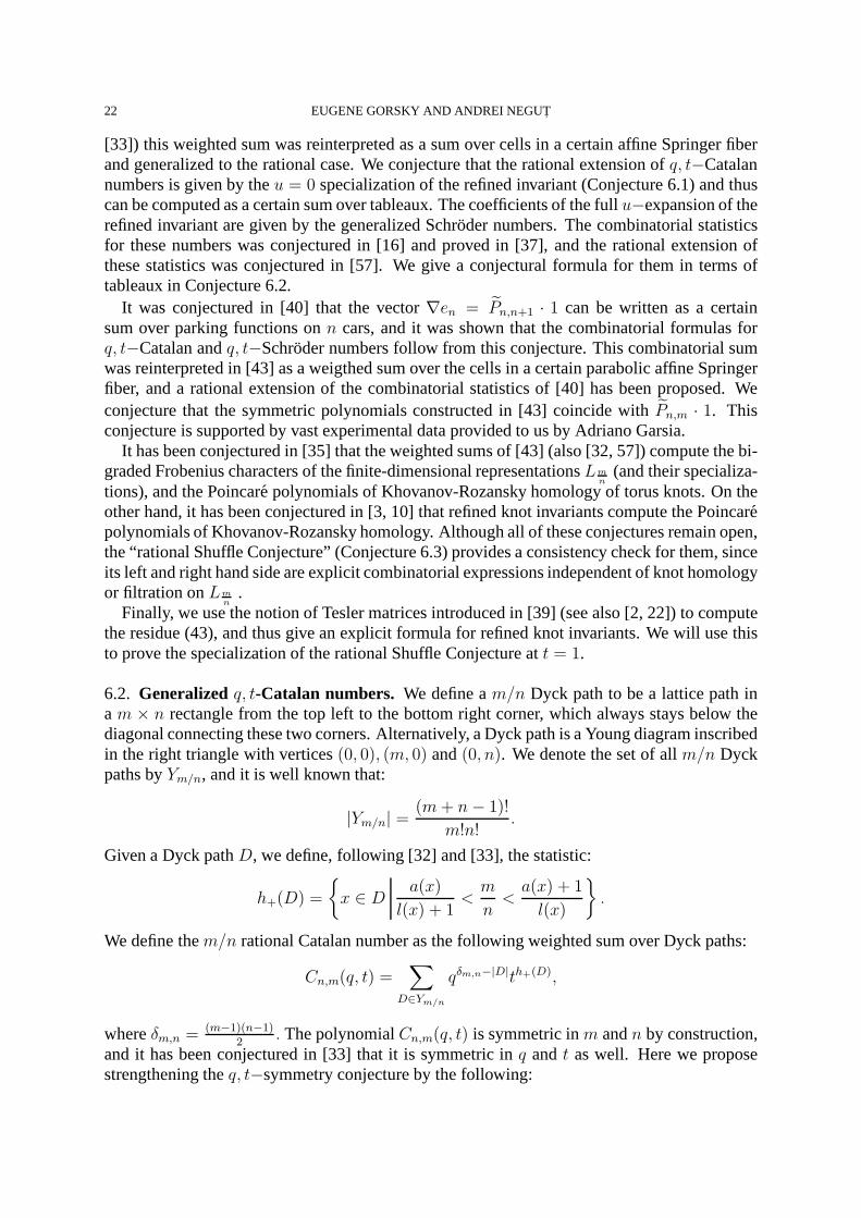
Given a Dyck pathD and an internal vertexP , we defineβ(P ) to be the number of horizontalsegments ofD intersected by the line passing throughP and parallel to the diagonal (see Figure3). Letv(D) denote the set of internal vertices ofD.

P•

FIGURE 3. Computation of the statisticβ(P )

Conjecture 6.2. The following equation holds:∑

D∈Ym/n

qδm,n−|D|th+(D)∏

P∈v(D)

(1− ut−β(P )) = Pn,m(u, q, t)

Form = n + 1 a similar identity was conjectured in [16] and proved in [37](see [38] and[57, Section A.3] for more details).

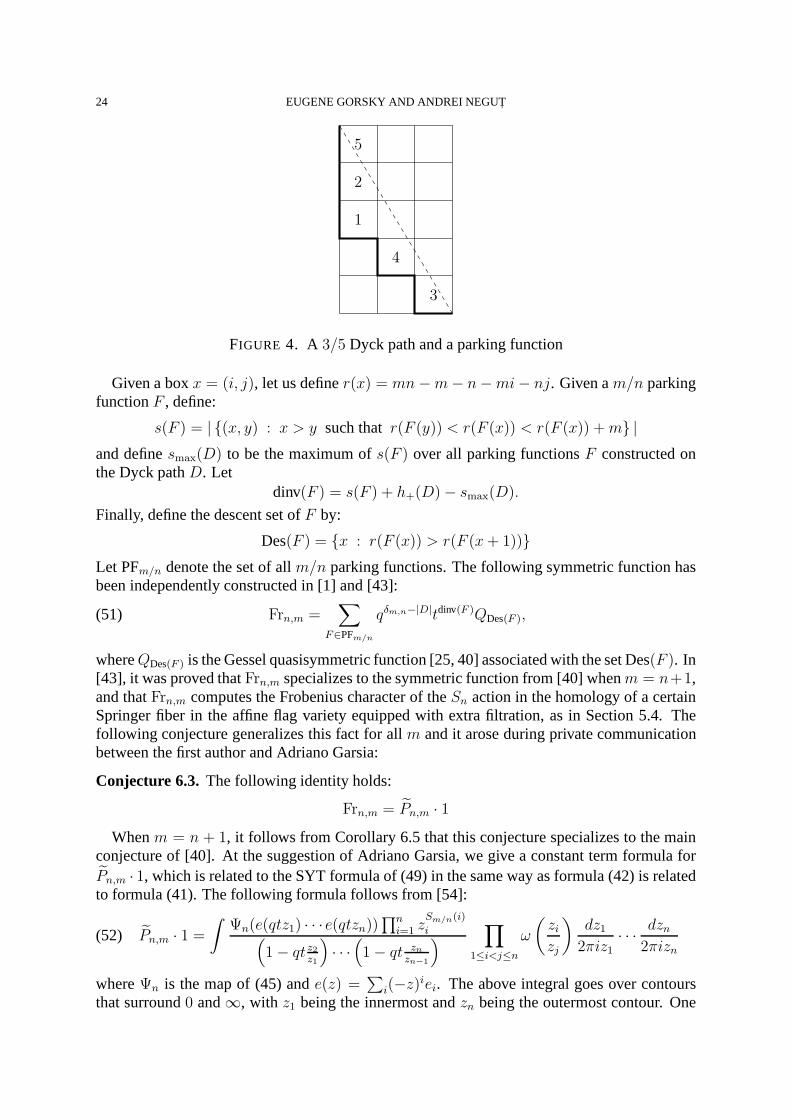
6.3. The Rational Shuffle Conjecture. The symmetric polynomialPn,m · 1 ∈ V has a com-binatorial interpretation. Let us define am/n parking function as a function:

f : {1, . . . , m} → {1, . . . , n}, such that|f−1([1, i])| ≥mi

n∀ i

Alternatively, a parking function can be presented as a standard Young tableauF of skewshape(D + 1m) \D, whereD is am/n Dyck path. Given such a tableau, the functionf canbe reconstructed by sending eachi to thex-coordinate of the box labeled byi in the tableau. Itis clear that this correspondence is bijective.


5

2

1

4

3

FIGURE 4. A 3/5 Dyck path and a parking function

Given a boxx = (i, j), let us definer(x) = mn−m− n−mi− nj. Given am/n parkingfunctionF , define:

s(F ) = | {(x, y) : x > y such thatr(F (y)) < r(F (x)) < r(F (x)) +m} |

and definesmax(D) to be the maximum ofs(F ) over all parking functionsF constructed onthe Dyck pathD. Let

dinv(F ) = s(F ) + h+(D)− smax(D).

Finally, define the descent set ofF by:

Des(F ) = {x : r(F (x)) > r(F (x+ 1))}

Let PFm/n denote the set of allm/n parking functions. The following symmetric function hasbeen independently constructed in [1] and [43]:

(51) Frn,m =∑

F∈PFm/n

qδm,n−|D|tdinv(F )QDes(F ),

whereQDes(F ) is the Gessel quasisymmetric function [25, 40] associated with the set Des(F ). In[43], it was proved thatFrn,m specializes to the symmetric function from [40] whenm = n+1,and thatFrn,m computes the Frobenius character of theSn action in the homology of a certainSpringer fiber in the affine flag variety equipped with extra filtration, as in Section 5.4. Thefollowing conjecture generalizes this fact for allm and it arose during private communicationbetween the first author and Adriano Garsia:

Conjecture 6.3. The following identity holds:

Frn,m = Pn,m · 1

Whenm = n + 1, it follows from Corollary 6.5 that this conjecture specializes to the mainconjecture of [40]. At the suggestion of Adriano Garsia, we give a constant term formula forPn,m · 1, which is related to the SYT formula of (49) in the same way as formula (42) is relatedto formula (41). The following formula follows from [54]:

(52) Pn,m · 1 =

∫Ψn(e(qtz1) · · · e(qtzn))

∏ni=1 z

Sm/n(i)

i(1− qtz2

z1

)· · ·(1− qt zn

zn−1

)∏

1≤i<j≤n

ω

(zizj

)dz12πiz1

· · ·dzn2πizn

whereΨn is the map of (45) ande(z) =∑

i(−z)iei. The above integral goes over contoursthat surround0 and∞, with z1 being the innermost andzn being the outermost contour. One


can compute the above residues inzi and produce a sum of symmetric functions indexed bycertain matrices of natural numbers. We will show how to do this in the slightly simpler caseof the super-polynomialsPn,m.

6.4. The m = n + 1 case.For m = n + 1, one can prove that the rationalq, t–Catalannumbers agree with theq, t–Catalan numbers defined in [23], and Conjecture 6.3 agrees withthe “Shuffle conjecture” of [40]. The following propositionfollows from the results of [23],but we present its proof here for completeness.

Proposition 6.4. One has the identity:P0,1(pn) = en.

Proof. It is enough to prove this above in anyVN , sinceV is the inverse limit of these vectorspaces. Let us recall that:

PN

0,k = t−k(N−1)

(PN0,k −

tkN − 1

tk − 1

)

If we keepN finite but make the change of variablesϕ 11−1/t

of Theorem 4.2, we obtain theoperator:

(53) PN0,1 = ϕ 1

1−1/t◦ P

N

0,1 ◦ ϕ−1

11−1/t

= t−N+1ϕ 11−1/t

◦

(δ1 −

tN − 1

t− 1

)◦ ϕ−1

11−1/t

whereδ1 is the operator of (11). The operatorsPN0,1 stabilize toP0,1. Using (53), we can rewrite

the desired identity as:

(54) δ1(pn) =1− tN

1− tpn + (−1)n

tN (1− qn)

tn(1− t)ϕ−1

11−1/t

(en).

Indeed,∂(i)q pn = pn + (qn − 1)xn

i , so by (11)

δ1(pn) = pn∑

i

Ai(x) + (qn − 1)∑

i

Ai(x)xni .

Consider the functionF (z) =∏N

i=11−zxi

1−ztxi=∑∞

z=0 znFn. It has the following partial fraction

decomposition:

F (z) =1

tN+

t− 1

tN

N∑

i=1

Ai(x)

1− tzxi

,

hence

(55)∑

i

Ai(x)xni =

{1−tN

1−tn = 0

FntN

tn(t−1)n > 0,

Therefore we have

δ1(pn) =1− tN

1− tpn +

tN(1− qn)

tn(1− t)Fn.

On the other hand,

lnF (z) =

N∑

i=1

(ln(1− zxi)− ln(1− ztxi)) = −

∞∑

k=1

(1− tk)zkpkk

,

hence

F (z) = ϕ−11

1−t

[exp(−

∞∑

k=1

zkpkk

)

]= ϕ−1

11−t

[∏

i

(1− zxi)

],


andFn = (−1)nϕ−11

1−t

(en). �

Corollary 6.5. The following identities hold:

Pn,1 · 1 = en, Pn,n+1 · 1 = ∇en

Proof. It follows from (22) thatPn,1 = [P0,1, Pn,0], hence:

Pn,1 · 1 = [P0,1, Pn,0] · 1 = P0,1Pn,0 · 1 = P0,1 · pn = en.

The second identity follows from the equationPn,n+1 = ∇Pn,1∇−1. �

As a corollary, we get the following decomposition of the Garsia-Haiman coefficients:

Proposition 6.6. Given a Young diagramλ, the following identity holds:

(56) ΠλBλ =1

M

SYT∑

T of shapeλ

cn,1(T ),

where:

Πλ =

χ(�)6=1∏

�∈λ

(1− χ(�)), Bλ =∑

�∈λ

χ(�)

The coefficientscn,1(T ) are defined by (50).

Proof. It has been shown in [23, Theorem 2.4] that the left hand side of (56) coincides with thecoefficient:

gλ · 〈en, Hλ〉q,t−1

By Corollary 6.5, this is equal togλ · 〈Hλ|Pn,1|1〉q,t−1, which equals the right hand side of (56)by (50). �

6.5. Tesler matrices. By (43), the super-polynomialsPn,m ultimately come down to comput-ing the residue:

Pn,m(u, q, t) = (Reszn=0 − Reszn=∞) · · · (Resz1=0 − Resz1=∞)

(57)1

z1 · · · zn·

∏ni=1 z

Sm/n(i)

i · 1−uzizi−1(

1− qtz2z1

)· · ·(1− qt zn

zn−1

)∏

1≤i<j≤n

ω

(zizj

)

Form > 0, the above only has residues atzi = ∞. Therefore, let us consider the expansions:

1− ux

x− 1= −1 + (u− 1)

∑

k≥1

x−k, ω(x) = 1 +∑

k=1

A(k)x−k,ω(x)

1− qtx

=∑

k=1

B(k)x−k

where:

A(k) = −(q − 1)(t− 1)qk − tk

q − t, B(k) =

(qk+1 − qk)− (tk+1 − tk)

q − t

Using these, we can compute the (57) inductively. Take first the residue in the variablez1:

Pn,m(u, q, t) =

xin≥0∑

x1n+...+xn

n=Sm/n(n)

(1− u+ uδ0xnn) · A(xn−1

n )

xin>0∏

i<n−1

B(xin)


Reszn=∞ · · ·Resz2=∞1

z1 · · · zn−1

∏ni=2 z

Sm/n(i)+x1i

i · 1−uzizi−1(

1− qtz2z1

)· · ·(1− qt zn

zn−1

)∏

1≤i<j≤n−1

ω

(zizj

)

Following [39] (see also [22] and [2]), we introduce the notion of Tesler matrix. An upper tri-angular matrixX = {xi

j ≥ 0}1≤i≤j≤n is called am/n Tesler matrix if it satisfies the followingsystem of equations:

(58) xii +∑

j>i

xij −

∑

j<i

xji = Sm/n(i) ∀ i

We will denote the set of allm/n Tesler matrices by Tesm/n. Taking next the residues in thevariablesz2, . . . , zn gives us:

(59) Pn,m(u, q, t) =∑

X∈Tesm/n

xii>0∏

1≤i≤n

(1− u)∏

1≤i≤n−1

B(xii+1)

xij>0∏

i<j−1

A(xij)

Therefore, the above computes the uncolored knot invariantas a sum of certain simple termsover all Tesler matrices. Note that the whole sum depends very strongly onn, while themdependence is captured only in the equation (58). However, the superpolynomialPn,m is con-jecturally symmetric inm andn, and this is not manifest from the above formula.

6.6. Degeneration att = 1. In fact, Pn,m|u=0 is a polynomial inq andt with positive coef-ficients, which is not manifest from (59) above. This followsfrom the fact that it is the Eulercharacteristic of a certain line bundle on the flag Hilbert schemeHilb0,n, as in Subsection 4.3.The higher cohomology groups of this line bundle vanish, andH0 only produces positive coef-ficients (this vanishing result is outside the scope of this paper and will be presented in a futurework). However, we can completely describe this polynomialwhen t = 1 (or whenq = 1,since the right hand side of (59) is clearly symmetric inq andt).

Theorem 6.7.Conjectures 6.1 and 6.2 hold fort = 1 and any coprimen,m.

Proof. Let us first remark that any Tesler matrix from Tesm,n gives rise to a Dyck path in then×m rectangle, with horizontal stepsxi

i. Indeed, for anyk ≤ n we have the equation:

Sm/n(1) + . . .+ Sm/n(k) =

k∑

i=1

(xii +∑

j>i

xij −

∑

j<i

xji

)=

k∑

i=1

(xii +∑

j>k

xij

)

Therefore:k∑

i=1

xii ≤ Sm/n(1) + . . .+ Sm/n(k) =

⌊km

n

⌋.

Any given Dyck path may correspond to many Tesler matrices. However, note that:

(60) A(x)|t=1 = δ0x, B(x)|t=1 = qx

so any summand of (59) that has somexij > 0 for j > i + 1 will vanish. Therefore, the only

summands of (59) that survive are those such thatxij = 0 for all j > i + 1. Such Tesler

matrices will be calledquasi-diagonal, and the set of quasi-diagonalm/n Tesler matrices willbe denoted by qTesm/n. Therefore, (59) becomes:

(61) Pn,m(0, q, 1) =∑

X∈qTesm/n

qxn−1n +...+x1

2

xii>0∏

1≤i≤n

(1− u)


The conditionxii > 0 specifies the corners of a Dyck path, while the sum

∑n−1i=1 xi

i+1 =∑ni=1 i(Sm/n(i)− xi

i) computes the area between the Dyck path and the diagonal. Therefore:

Pn,m(0, q, 1) =∑

D∈Ym/n

q(m−1)(n−1)

2−|D|(1− u)# of corners ofD

This implies Conjecture 6.2 att = 1. When we setu = 0, we obtain Conjecture 6.1 att = 1.�

6.7. Degeneration att = q−1. We will compute the knot invariant att = q−1, and show thatit is a q−analogue of them,n−Catalan number. This proves Conjecture 6.1 att = q−1.

Proposition 6.8. For anym andn with gcd(m,n) = 1, we have:

(62) Pn,m(0, q, q−1) =

[m+ n− 1]!

[m]![n]!,

where[k] = qk/2−q−k/2

q1/2−q−1/2 are theq−integers and[k]! = [1] · · · [k] are theq−factorials.

Proof. Let us describe the degeneration of all constructions that we used to the caset = q−1,whereq andt are the equivariant parameters onC

2. Macdonald polynomialsPλ(q, t−1) will de-

generate to Schur polynomialssλ, hence modified Macdonald polynomialsHλ will degenerateto modified Schur polynomialsϕ 1

1−1/t(sλ).

As it was explained in [3], the caset = q−1 corresponds to the classical Chern-Simons theory.The corresponding knot invariants and operators were widely discussed in the mathematical andphysical literature, see e.g. [48, 63] for more details. In particular, it is shown in [63, section3.4] that:

Pn,m(q, q−1) = DPn,0(q, q

−1)D−1, whereD = ∇(q, q−1)mn .

Remark thatpn =∑n−1

k=0(−1)ks(n−k,1k), and:

∇(s(n−k,1k)) = q(n−k)(n−k−1)

2− k(k+1)

2 s(n−k,1k) = qn(n−2k−1)

2 s(n−k,1k),

hence:D(s(n−k,1k)) = q

m(n−2k−1)2 s(n−k,1k) = q

(m−1)(n−1)2

+n−12

−kms(n−k,1k).

Therefore:

Pn,m(1) = D(pn) = q(m−1)(n−1)

2

n−1∑

k=0

(−1)kqn−12

−kmϕ 11−1/t

(s(n−k,1k)).

By [4, Theorem 1.6], this vector coincides with the graded Frobenius character of the finite-dimensional representationLm/n. One can also check (see e.g [30, 35] for details) that itsevaluation is given by the equation (62). �

REFERENCES

[1] D. Armstrong. Rational Catalan Combinatorics, slides from a talk at JMM 2012, Boston.[2] D. Armstrong, A. Garsia, J. Haglund, B. Rhoades, and B. Sagan. Combinatorics of Tesler matrices in the

theory of parking functions and diagonal harmonics. J. Comb. 3 (2012), no. 3, 451-494.[3] M. Aganagic, S. Shakirov. Knot Homology from Refined Chern-Simons Theory. arXiv:1105.5117.[4] Yu. Berest, P. Etingof, V. Ginzburg, Finite-dimensional representations of rational Cherednik algebras, Int.

Math. Res. Not. 2003, no. 19, 1053–1088.[5] F. Bergeron, A. Garsia. Science Fiction and Macdonald’sPolynomials, CRM Proceedings& Lecture Notes,

American Mathematical Society , 22, 1–52, 1999[6] F. Bergeron, A. Garsia, E. Leven, G. Xin. Compositional(km, kn)–Shuffle Conjectures. arXiv:1404.4616

http://arxiv.org/abs/1105.5117



[7] R. Bezrukavnikov, M. Finkelberg, V. Ginzburg, Cherednik algebras and Hilbert schemes in characteristicp,Represent. Theory10 (2006), 254–298

[8] I. Burban, O. Schiffmann, On the Hall algebra of an elliptic curve, I. Duke Math. J.161 (2012), no. 7,1171–1231

[9] M. Can. Nested Hilbert schemes and the nestedq, t-Catalan series. arXiv:0711.0763[10] I. Cherednik, Jones polynomials of torus knots via DAHA, Int. Math. Res. Not. IMRN 2013, no. 23, 5366–

5425.[11] I. Cherednik. Macdonald’s evaluation conjectures anddifference Fourier transform. Invent. Math.122

(1995), no. 1, 119–145.[12] I. Cherednik. Double affine Hecke algebras and Macdonald’s conjectures. Ann. of Math. (2)141(1995), no.

1, 191–216.[13] I. Cherednik. Irreducibility of perfect representations of double affine Hecke algebras. Studies in Lie theory,

79–95, Progr. Math.,243, Birkhauser Boston, Boston, MA, 2006.[14] I. Cherednik. Double affine Hecke algebras. London Mathematical Society Lecture Note Series, 319. Cam-

bridge University Press, Cambridge, 2005.[15] P. Dunin-Barkowski, A. Mironov, A. Morozov, A. Sleptsov, A. Smirnov. Superpolynomials for toric knots

from evolution induced by cut-and-join operators. J. High Energy Phys. 2013, no. 3, 021, front matter+85pp.

[16] E. Egge, J. Haglund, D. Kremer, K. Killpatrick. A Schroder generalization of Haglund’s statistic on Catalanpaths. Electron. J. of Combin., 10 (2003), Research Paper 16, 21 pages.

[17] P. Etingof, V. Ginzburg. Symplectic reflection algebras, Calogero-Moser space, and deformed Harish-Chandra homomorphism. Invent. Math.147(2002), no. 2, 243–348.

[18] P. Etingof, E. Gorsky, I. Loseu. Representations of Rational Cherednik algebras with minimal support andtorus knots. arXiv:1304.3412

[19] P. Etingof, A. Kirillov Jr. Representation-theoreticproof of the inner product and symmetry identities forMacdonald’s polynomials. Compositio Math.102(1996), no. 2, 179–202

[20] B. Feigin, A. Tsymbaliuk, Heisenberg action in the equivariant K-theory of Hilbert schemes via shufflealgebra. Kyoto J. Math.51 (2011), no. 4, 831854.

[21] A. Garsia, J. Haglund. A proof of theq, t-Catalan positivity conjecture. Discrete Math.,256(2002), 677–717.[22] A. Garsia, J. Haglund, G. Xin. Constant term methods in the theory of Tesler matrices and Macdonald

polynomial operators. Ann. Comb.18 (2014), no. 1, 83–109.[23] A. Garsia, M. Haiman. A remarkableq, t-Catalan sequence andq-Lagrange inversion. J. Algebraic Combin.

5 (1996), no. 3, 191–244.[24] A. Garsia, M. Haiman. A graded representation model forMacdonald’s polynomials. Proc. Nat. Acad. Sci.

U.S.A.90 (1993), no. 8, 3607–3610.[25] I. Gessel. MultipartiteP -partitions and inner products of skew Schur functions. In:Combinatorics and alge-

bra Contemp. Math.34, 289–317. Amer. Math. Soc., Providence, RI, 1984.[26] I. Gordon. On the quotient ring by diagonal invariants.Invent. Math.153(2003), no. 3, 503–518.[27] I. Gordon, T. Stafford, Rational Cherednik algebras and Hilbert schemes, Advances in Mathematics198.1

(2005), 222–274.[28] I. Gordon, T. Stafford, Rational Cherednik algebras and Hilbert schemes II: representations and sheaves,

Duke Math. J.132.1 (2006), 73–135.[29] M. Goresky, R. Kottwitz, R. MacPherson. Purity of equivalued affine Springer fibers. Represent. Theory10

(2006), 130–146.[30] E. Gorsky.q, t–Catalan numbers and knot homology. Zeta Functions in Algebra and Geometry, 213–232.

Contemp. Math.566, Amer. Math. Soc., Providence, RI, 2012.[31] E. Gorsky. Arc spaces and DAHA representations. Selecta Mathematica, New Series,19 (2013), no. 1, 125–

140.[32] E. Gorsky, M. Mazin. Compactified Jacobians andq, t-Catalan Numbers, I. Journal of Combinatorial Theory,

Series A,120(2013) 49–63.[33] E. Gorsky, M. Mazin. Compactified Jacobians andq, t-Catalan Numbers, II. J. Algebraic Combin.39(2014),

no. 1, 153–186.[34] E. Gorsky, M. Mazin, M. Vazirani. Affine permutations and rational slope parking functions. To appear in

Transactions of the AMS.




[35] E. Gorsky, A. Oblomkov, J. Rasmussen, V. Shende. Torus knots and the rational DAHA. Duke Math. J.163(2014), no. 14, 2709–2794.

[36] J. Haglund. Conjectured statistics for the(q, t)-Catalan numbers , Adv. Math.175(2003), 319–334.[37] J. Haglund. A proof of theq, t-Schroder conjecture. Internat. Math. Res. Notices,11 (2004), pp. 525–560.[38] J. Haglund. Theq, t-Catalan Numbers and the Space of Diagonal Harmonics: With an Appendix on the

Combinatorics of Macdonald Polynomials. AMS University Lecture Series41 (2008).[39] J. Haglund. A polynomial expression for the Hilbert series of the quotient ring of diagonal coinvariants ,

Adv. Math.,227(2011), 2092–2106.[40] J. Haglund, M. Haiman, N. Loehr, J. Remmel, A. Ulyanov. Acombinatorial formula for the character of the

diagonal coinvariants. Duke Math. J. ,126(2005), 195–232.[41] M. Haiman. Vanishing theorems and character formulas for the Hilbert scheme of points in the plane , Invent.

Math.149.2 (2002), 371-407.[42] M. Haiman. Combinatorics, symmetric functions and Hilbert schemes. Current Developments in Mathemat-

ics 2002, no. 1, 39–111.[43] T. Hikita. Affine Springer fibers of typeA and combinatorics of diagonal coinvariants. Adv. Math.263

(2014), 88–122.[44] M. Kashiwara, R. Rouquier. Microlocalization of rational Cherednik algebras. Duke Math. J.144(2008), no.

3, 525–573.[45] D. Kazhdan, G. Lusztig. Fixed point varieties on affine flag manifolds. Israel J. Math.62 (1988), no. 2,

129–168.[46] M. Khovanov. Triply-graded link homology and Hochschild homology of Soergel bimodules. Internat. J.

Math.18 (2007), no. 8, 869–885.[47] M. Khovanov, L. Rozansky. Matrix factorizations and link homology. II. Geom. Topol.12 (2008), no. 3,

1387-1425.[48] A. Kirillov Jr. On an inner product in modular tensor categories. J. Amer. Math. Soc.9 (1996), no. 4, 1135–

1169.[49] G. Lusztig, J. M. Smelt. Fixed point varieties on the space of lattices. Bull. London Math. Soc. 23 (1991),

no. 3, 213218.[50] I. G. Macdonald, Symmetric Functions and Hall Polynomials. Oxford Mathematical Monographs, second

ed., Oxford Science Publications. The Clarendon Press Oxford University Press, New York, 1995.[51] H. Morton, P. Samuelson. The HOMFLYPT skein algebra of the torus and the elliptic Hall algebra.

arXiv:1410.0859[52] H. Nakajima. Lectures on Hilbert schemes of points on surfaces. University Lecture Series,18. American

Mathematical Society, Providence, RI, 1999.[53] H. Nakajima. Refined Chern-Simons theory and Hilbert schemes of points on the plane. arXiv:1211.5821[54] A. Negut,, Moduli of Flags of Sheaves onP2 and theirK−theory. arXiv:1209.4242[55] A. Negut,. The m

n−Pieri rule. arXiv:1407.5303

[56] A. Negut,. The Shuffle Algebra Revisited. arXiv:1209.3349[57] A. Oblomkov, J. Rasmussen, V. Shende. The Hilbert scheme of a plane curve singularity and the HOMFLY

homology of its link, with the appendix of E. Gorsky. arXiv:1201.2115[58] A. Oblomkov, Z. Yun. Geometric representations of graded and rational Cherednik algebras.

arXiv:1407.5685[59] A. Okounkov, R. Pandharipande. The quantum differential equation of the Hilbert scheme of points in the

plane. Transform. Groups15 (2010), no. 4, 965–982.[60] O. Schiffmann, E. Vasserot. The elliptic Hall algebra and the K-theory of the Hilbert scheme ofA2. Duke

Math. J. 162 (2013), no. 2, 279366.[61] O. Schiffmann, E. Vasserot. The elliptic Hall algebra,Cherednik Hecke algebras and Macdonald polynomi-

als. Compos. Math.147(2011), no. 1, 188234.[62] S. Shakirov. Beta Deformation and Superpolynomials of(n,m) Torus Knots. arXiv:1111.7035[63] S. Stevan. Chern-Simons invariants of torus links. Ann. Henri Poincare11 (2010), no. 7, 1201–1224.[64] M. Varagnolo, E. Vasserot. Finite-dimensional representations of DAHA and affine Springer fibers: the

spherical case. Duke Math. J.147(2009), no. 3, 439–540.

DEPARTMENT OFMATHEMATICS, COLUMBIA UNIVERSITY, 2990 BROADWAY , NEW YORK, NY 10027

DEPARTMENT OFMATHEMATICS, UC DAVIS , ONE SHIELDS AVE, DAVIS , CA 95616










INTERNATIONAL LABORATORY OF REPRESENTATIONTHEORY AND MATHEMATICAL PHYSICS, NRU-HSE, 7 VAVILOVA ST., MOSCOW, RUSSIA 117312

E-mail address: [email protected]

MATHEMATICS DEPARTMENT, COLUMBIA UNIVERSITY, NEW YORK, NY 10027, USA

SIMION STOILOW INSTITUTE OFMATHEMATICS, BUCHAREST, ROMANIA

E-mail address: [email protected]

Documents

UC Davis - CORE