UC Irvine - CORE

UC IrvineUC Irvine Electronic Theses and Dissertations

TitleAlternative Light- and Heavy-Duty Vehicle Fuel Pathway and Powertrain Optimization

Permalinkhttps://escholarship.org/uc/item/70036475

AuthorLane, Blake

Publication Date2019 Peer reviewed|Thesis/dissertation

eScholarship.org Powered by the California Digital LibraryUniversity of California

https://escholarship.org/uc/item/70036475

https://escholarship.org

http://www.cdlib.org/

UNIVERSITY OF CALIFORNIA,

IRVINE

Alternative Light- and Heavy-Duty Vehicle Fuel Pathway and Powertrain Optimization

DISSERTATION

submitted in partial satisfaction of the requirements

for the degree of

DOCTOR OF PHILOSOPHY

in Mechanical and Aerospace Engineering

by

Blake Alexander Lane

Dissertation Committee:

Professor G. Scott Samuelsen, Chair

Dean Gregory N. Washington

Professor Stephen G. Ritchie

2019

© 2019 Blake Alexander Lane

ii

DEDICATION

To Tracy

iii

TABLE OF CONTENTS

LIST OF FIGURES ...................................................................................................................... vii

LIST OF TABLES ....................................................................................................................... xiv

NOMENCLATURE .................................................................................................................... xvi

ACKNOWLEDGMENTS ........................................................................................................... xix

CURRICULUM VITAE ............................................................................................................... xx

ABSTRACT OF THE DISSERTATION ................................................................................... xxii

1. INTRODUCTION ...................................................................................................................... 1

1.1 Motivation ............................................................................................................................. 1

1.2 Goal ....................................................................................................................................... 5

1.3 Objectives .............................................................................................................................. 5

2. BACKGROUND ........................................................................................................................ 7

2.1 Vehicle Fuels ......................................................................................................................... 7

2.1.1 Fuel Feedstocks ............................................................................................................... 8

2.1.2 Fuel Production ............................................................................................................. 10

2.1.3 Fuel Distribution ........................................................................................................... 34

2.1.4 Fuel Dispensing ............................................................................................................. 38

2.1.5 Fuel Emissions .............................................................................................................. 42

2.2 Vehicle Powertrains ............................................................................................................. 43

2.2.1 ICV ................................................................................................................................ 47

2.2.2 HEV ............................................................................................................................... 48

2.2.3 PHEV ............................................................................................................................ 48

2.2.4 BEV ............................................................................................................................... 49

2.2.5 FCEV ............................................................................................................................. 51

2.2.6 PFCEV .......................................................................................................................... 53

2.2.7 Vehicle Components ..................................................................................................... 55

2.3 Optimization and Linear Programming ............................................................................... 56

2.4 Literature Review ................................................................................................................ 60

2.4.1 Literature Review of Individual or Multiple Fuel Pathways Compared ....................... 60

2.4.2 Literature Review of Supply Chain Optimization......................................................... 66

2.4.3 Background Summary ...................................................................................................... 70

3. APPROACH ............................................................................................................................. 71

iv

3.1 Tasks .................................................................................................................................... 71

4. VEHICLE FUEL PATHWAYS ............................................................................................... 75

4.1 Fuel Feedstocks ................................................................................................................... 75

4.1.1 Electricity as a Fuel Feedstock ...................................................................................... 76

4.1.2 Biomass as a Fuel Feedstock ......................................................................................... 77

4.2 Fuel Production.................................................................................................................... 81

4.2.1 Hydrogen Fuel Production ............................................................................................ 83

4.2.2 SNG Fuel Production .................................................................................................... 98

4.2.3 Renewable Gasoline and Diesel Production ............................................................... 110

4.3 Fuel Distribution ................................................................................................................ 112

4.3.1 Electricity Distribution ................................................................................................ 112

4.3.2 Hydrogen Distribution ................................................................................................ 113

4.3.3 SNG Distribution......................................................................................................... 115

4.3.4 Renewable Gasoline and Diesel Distribution.............................................................. 116

4.4 Fuel Dispensing ................................................................................................................. 117

4.4.1 Electricity Dispensing ................................................................................................. 117

4.4.2 Hydrogen Dispensing .................................................................................................. 118

4.4.3 SNG Dispensing .......................................................................................................... 119

4.4.4 Renewable Gasoline and Diesel Dispensing ............................................................... 120

4.5 Total Fuel Pathway Efficiency and Emissions .................................................................. 121

4.5.1 Total Fuel Pathway Efficiency .................................................................................... 121

4.5.2 Feedstock Emissions ................................................................................................... 122

5. VEHICLE POWERTRAIN CONFIGURATIONS ................................................................ 131

5.1 Vehicle Efficiencies ........................................................................................................... 131

5.2 Vehicle Costs ..................................................................................................................... 135

5.3 Vehicle Tailpipe Emissions Factors .................................................................................. 137

5.3.1 LDV Tailpipe Emission Factors .................................................................................. 138

5.3.2 HDV Tailpipe Emission Factors ................................................................................. 139

6. MODEL CONSTRAINTS ...................................................................................................... 141

6.1 California GHG Emissions Goals...................................................................................... 141

6.2 Vehicle Miles Traveled ..................................................................................................... 142

6.2.1 Utility Factor ............................................................................................................... 148

6.2.2 Vehicle Fleet Turnover Rate ....................................................................................... 149

6.3 Technology Deployment ................................................................................................... 153

v

6.3.1 Electrolyzer Cumulative Production Limits ................................................................ 154

6.3.2 Biomass Feedstock Fuel Production Equipment Cumulative Production Limits ....... 157

6.3.3 Future Vehicle Powertrain Availabilities .................................................................... 158

6.4 Fuel Feedstock Availability ............................................................................................... 159

7. ESTABLISHING THE OPTIMIZATION PROBLEM.......................................................... 162

7.1 Optimization Method ......................................................................................................... 162

7.2 Cost Function ..................................................................................................................... 163

7.3 Constraints ......................................................................................................................... 167

7.4 Cost and Efficiency Updates ............................................................................................. 171

8. OPTIMAL FUEL AND VEHICLE DEPLOYMENT ............................................................ 172

8.1 Reference Case .................................................................................................................. 172

8.2 TRACE Non-ZEV Constrained Case ................................................................................ 177

8.3 Comparison of Reference Case and TRACE Non-ZEV Constrained Case ...................... 186

8.4 Additional Constraints ....................................................................................................... 190

8.4.1 Effect of ZEV Constraints ........................................................................................... 190

8.4.2 Effect of Drayage CAP Emissions Constraints ........................................................... 197

8.5 Sensitivity Analyses .......................................................................................................... 203

8.5.1 Effect of Continued Production Plant Constraint ........................................................ 204

8.5.2 Effect of Electricity Distribution Cost ........................................................................ 208

8.5.3 Effect of Electricity Dispensing Cost .......................................................................... 209

8.5.4 Effect of Electrolyzer Technology Cost ...................................................................... 209

8.5.5 Effect of Gasifier Cost................................................................................................. 210

8.5.6 Effect of Fuel Cell Cost ............................................................................................... 210

8.5.7 Effect of Liquefaction Cost ......................................................................................... 210

8.5.8 Effect of Electricity Feedstock Constraints ................................................................. 215

8.5.9 Effect of CF and Electricity Cost on P2G Technology ............................................... 217

8.5.10 Effect of Battery Learning Rate ................................................................................ 217

8.5.11 Effect of VMT Changes ............................................................................................ 222

9. SUMMARY AND CONCLUSIONS ..................................................................................... 239

9.1 Summary ............................................................................................................................ 239

9.2 Conclusions ....................................................................................................................... 241

9.2.1 LDV Conclusions ........................................................................................................ 241

9.2.2 HDV Conclusions ....................................................................................................... 242

9.2.3 General Conclusions ................................................................................................... 243

vi

9.3 Future Work ....................................................................................................................... 246

10. REFERENCES ..................................................................................................................... 249

11. APPENDIX A ....................................................................................................................... 272

12. APPENDIX B ....................................................................................................................... 278

vii

LIST OF FIGURES

Figure 1. Left chart: U.S. GHG emissions per economic sector in 2016, from U.S.

EPA [1]; Right chart: Global GHG emissions per economic sector in

2014, from U.S. EPA [2] 2

Figure 2. Electricity Sources in California in February 2019, from U.S. Energy

Information Administration [34]................................................................12

Figure 3. Schematic of P2G Pathways, from the Advanced Power and Energy

Program [38] ..............................................................................................15

Figure 4. Flowchart of analyzed electrolytic hydrogen production pathways ..........16

Figure 5. Methanator equilibrium species concentrations at 5atm ............................21

Figure 6. Flowchart of analyzed electrolytic SNG production pathways .................22

Figure 7. Liquefaction fuel production diagram for renewable gasoline and

renewable diesel, from U.S. Department of Energy [120] ........................31

Figure 8. Gasification and Fischer-Tropsch production diagram for renewable

gasoline and diesel, from U.S. Department of Energy [122] .....................32

Figure 9. Flow diagram of fuel production pathways ...............................................34

Figure 10. Diagram of electricity transmission and distribution network, from

U.S. Energy Information Administration [123] .........................................35

Figure 11. PEV charging connectors for level 3 on the left and levels 1 and 2 on

the right, from U.S. Department of Energy [129] ......................................40

Figure 12. SNG dispensing station schematic, from U.S. Department of Energy

[138] ...........................................................................................................42

Figure 13. Annual VMT by vehicle category, from U.S. Department of Energy

[140] ...........................................................................................................44

Figure 14. California new vehicle registrations in first half of 2018, data from

[142] ...........................................................................................................45

Figure 15. Schematic of PEM Fuel Cell, from U.S. Department of Energy [158] .....52

Figure 16. Simplified powertrain schematic of PFCEV..............................................54

Figure 17. Sankey diagram for US Energy consumption, from U.S. Department

of Energy [168] ..........................................................................................57

viii

Figure 18. Electricity price projections, current policy reference scenario with

SB 100, from [189] ....................................................................................76

Figure 19. Current and potential biomass production for energy use in California

based on medium housing, medium energy use, and base case energy

crop growth scenario with non-organic MSW removed, data from [31]. ..78

Figure 20. Total biomass energy available by feedstock category, data from [31] ....79

Figure 21. Probability distribution of 108 studies that report learning rates in 22

industrial sectors from [196] ......................................................................82

Figure 22. Range of electrolyzer efficiencies found in the literature, from sources

of Table 8 ...................................................................................................84

Figure 23. Electrolyzer system efficiency projections from [37], [170], [203] ..........85

Figure 24. Conservative estimate on electrolyzer efficiency projection .....................86

Figure 25. Optimistic estimate on electrolyzer efficiency projection .........................87

Figure 26. Information on cost for PEMEC and AEC versus time for references

listed in Table 9 ..........................................................................................88

Figure 27. More detailed information on cost for AEC versus time for [206] and

[37] to show difference between survey information and experience

curve calculations.......................................................................................89

Figure 28. Conservative projection of cost and representative electrolyzer market

size .............................................................................................................91

Figure 29. Optimistic projection of installed cost and representative electrolyzer

market size .................................................................................................92

Figure 30. Detailed view of electrolyzer cost projections ...........................................93

Figure 31. Conservative projection of installed cost compared with literature

projections ..................................................................................................94

Figure 32. Optimistic projection of installed cost compared with literature

projections ..................................................................................................94

Figure 33. Gasification efficiency ranges and average for hydrogen production,

data from [41], [42], [51], [52], [43]–[50] .................................................96

Figure 34. Efficiency projections of gasification for hydrogen production ................96

Figure 35. Gasification cost ranges and average for hydrogen production, data

from [41][42][43], [44][45]–[52] ...............................................................97

ix

Figure 36. Cost projection for gasification production of hydrogen ...........................98

Figure 37. Efficiency of anaerobic digestion, categorized by feedstock, with

data from [84], [222], [231]–[236], [223]–[230] .....................................104

Figure 38. Efficiency projections for anaerobic digestion of manure feedstocks .....105

Figure 39. Efficiency projections for anaerobic digestion of organic feedstocks .....105

Figure 40. Installed cost of anaerobic digestion, categorized by feedstock, data

from [84], [222]–[225], [237]–[241] .......................................................106

Figure 41. Cost projections for anaerobic digestion..................................................107

Figure 42. Gasification efficiency ranges and average for SNG production, data

from [86], [87], [96]–[104], [88]–[95][105], [106], [115], [116],

[107]–[114]. .............................................................................................108

Figure 43. Efficiency projections for gasification for SNG production ....................108

Figure 44. Gasification cost ranges and average for SNG production, data from

[84], [222]–[225], [237]–[241] ................................................................109

Figure 45. Cost projections for gasification for SNG production .............................110

Figure 46. Levelized cost of hydrogen distribution and dispensing, data from

[252] .........................................................................................................115

Figure 47. Feedstock carbon intensities ....................................................................126

Figure 48. Electricity GHG and CAP emissions, data from [31], [189] ...................129

Figure 49. Biomass feedstock availability by individual feedstock, data from

[31] ...........................................................................................................130

Figure 50. California GHG emissions regulations and the current state, from

[275][7], [9], [10] .....................................................................................142

Figure 51. LDV VMT projections with NHTS/ARB data from [277] [278] and

EMFAC data from [141] ..........................................................................144

Figure 52. HDV VMT projection by vocation, data from [141] ...............................145

Figure 53. LDV fleet turnover by VMT, data from [141] .........................................151

Figure 54. Linehaul HDV fleet turnover by VMT, data from [141] .........................151

Figure 55. Drayage HDV fleet turnover by VMT, data from [141] ..........................152

x

Figure 56. Refuse HDV fleet turnover by VMT, data from [141] ............................152

Figure 57. Construction HDV fleet turnover by VMT, data from [141] ...................153

Figure 58. Future electrolyzer market size projections in 2030, 2035, and 2050

(based on assumed efficiency of 50kWh/kg and capacity factor of

90%) .........................................................................................................155

Figure 59. Future electrolyzer market size projections in 2030, 2035, and 2050

(based on assumed efficiency of 50kWh/kg and capacity factor of

50%) .........................................................................................................156

Figure 60. Conservative estimate on electrolyzer cumulative production limits ......156

Figure 61. Optimistic estimate on electrolyzer cumulative production limits ..........157

Figure 62. Biomass feedstock fuel production equipment cumulative production

limits ........................................................................................................158

Figure 63. Fuel feedstock availability, data from [189] and [31] ..............................161

Figure 64. Fossil fuel price projections, data from [296] ..........................................173

Figure 65. Reference Case LDV miles traveled ........................................................174

Figure 66. Reference Case HDV miles traveled by vocation....................................175

Figure 67. Reference Case emissions .......................................................................176

Figure 68. Reference Case cumulative cost ..............................................................177

Figure 69. TRACE Non-ZEV Constrained Case LDV miles traveled ......................178

Figure 70. TRACE Non-ZEV Constrained Case HDV miles traveled by vocation .179

Figure 71. TRACE Non-ZEV Constrained Case fuels used .....................................180

Figure 72. TRACE Non-ZEV Constrained Case feedstocks used ............................181

Figure 73. TRACE Non-ZEV Constrained Case fuel production equipment used ...182

Figure 74. TRACE Non-ZEV Constrained Case emissions......................................183

Figure 75. TRACE Non-ZEV Constrained Case cumulative cost ............................184

Figure 76. Comparison of cumulative cost for Reference Case and TRACE

Non-ZEV Constrained Case ....................................................................187

xi

Figure 77. GHG emissions comparison between Reference Case and TRACE


Figure 78. NOx emissions comparison between Reference Case and TRACE


Figure 79. PM10 emissions comparison between Reference Case and TRACE


Figure 80. Light-duty ZEV constraint LDV miles traveled ......................................190

Figure 81. Light-duty ZEV constraint HDV miles traveled ......................................191

Figure 82. Light-duty ZEV constraint fuels used ......................................................192

Figure 83. Light-duty ZEV constraint feedstocks used .............................................192

Figure 84. Light-duty ZEV constraint fuel production equipment used ...................193

Figure 85. Light-duty ZEV constraint emissions ......................................................194

Figure 86. All ZEV constraint fuels used ..................................................................195

Figure 87. All ZEV constraint fuel feedstocks used .................................................195

Figure 88. All ZEV constraint fuel production equipment use .................................196

Figure 89. All ZEV constraint emissions ..................................................................197

Figure 90. Drayage CAP emissions constraints LDV miles traveled .......................199

Figure 91. Drayage CAP emissions constraints HDV miles traveled .......................200

Figure 92. Drayage CAP emissions constraints fuels used .......................................201

Figure 93. Drayage CAP emissions constraints feedstocks used ..............................201

Figure 94. Drayage CAP emissions constraints fuel production equipment used ....202

Figure 95. Drayage CAP emissions constraints emissions .......................................203

Figure 96. No continued production plant constraint LDV miles traveled ...............204

Figure 97. No continued production plant constraint HDV miles traveled by

vocation ....................................................................................................205

Figure 98. No continued production plant constraint fuels used ...............................206

Figure 99. No continued production plant constraint feedstocks used......................206

xii

Figure 100. No continued production plant constraint fuel production equipment

used ..........................................................................................................207

Figure 101. No continued production plant constraint emissions ...............................208

Figure 102. Doubled liquefaction cost LDV miles traveled .......................................211

Figure 103. Doubled liquefaction cost HDV miles traveled by vocation ...................212

Figure 104. Doubled liquefaction cost fuels used .......................................................213

Figure 105. Doubled liquefaction cost feedstocks used ..............................................213

Figure 106. Doubled liquefaction cost fuel production equipment used ....................214

Figure 107. Doubled liquefaction cost emissions .......................................................215

Figure 108. Reduction of electricity feedstock availability by 57% fuels used ..........216

Figure 109. Reduction of electricity feedstock availability by 57% feedstocks used .216

Figure 110. Zero battery LR LDV miles traveled .......................................................218

Figure 111. Zero battery LR HDV miles traveled by vocation ...................................219

Figure 112. Zero battery LR fuels used .......................................................................220

Figure 113. Zero battery LR feedstocks used ..............................................................220

Figure 114. Zero battery LR fuel production equipment used ....................................221

Figure 115. Zero battery LR emissions .......................................................................222

Figure 116. Decrease in all VMT by 50% LDV miles traveled ..................................224

Figure 117. Decrease in all VMT by 50% HDV miles traveled .................................225

Figure 118. Decrease in all VMT by 50% fuels used .................................................226

Figure 119. Decrease in all VMT by 50% feedstocks used ........................................226

Figure 120. Decrease in all VMT by 50% fuel production equipment used ...............227

Figure 121. Decrease in all VMT by 50% fuel production equipment used ...............228

Figure 122. Increase in all VMT by 50% LDV miles traveled ...................................229

Figure 123. Increase in all VMT by 50% HDV miles traveled ...................................230

Figure 124. Increase in all VMT by 50% fuels used ...................................................231

xiii

Figure 125. Increase in all VMT by 50% feedstocks used ..........................................231

Figure 126. Increase in all VMT by 50% fuel production equipment used ................232

Figure 127. Increase in all VMT by 50% emissions ...................................................233

Figure 128. Increase in light-duty VMT by 96% and heavy-duty VMT by 50%

LDV miles traveled ..................................................................................234


HDV miles traveled by vocation ..............................................................235


fuels used .................................................................................................236


feedstocks used ........................................................................................236


fuel production equipment used ...............................................................237


emissions ..................................................................................................238

xiv

LIST OF TABLES

Table 1. California transportation legislation and goals ...................................................... 3

Table 2. Biomass feedstocks by crop type according to Billion Ton Report [31] ............... 9

Table 3. Heat sink TRLs .................................................................................................... 23

Table 4. Carbon dioxide source TRLs ............................................................................... 24

Table 5. Vehicle components considered .......................................................................... 55

Table 6. Individual or Multiple Fuel Pathways Compared Literature Review .................. 64

Table 7. Supply Chain Optimization Literature Review.................................................... 69

Table 8. Information on efficiency for SOEC, PEMEC, and AEC from literature ........... 84

Table 9. Information on cost for PEMEC, SOEC, and AEC from literature ..................... 88

Table 10. Conservative projection of installed cost and representative electrolyzer

market size ........................................................................................................... 91

Table 11. Optimistic projection of installed cost and representative electrolyzer

market size ........................................................................................................... 92

Table 12. Methanator cost projections by market size....................................................... 100

Table 13. Conservative projection of carbon capture technology cost by market size ...... 101

Table 14. Optimistic projection of carbon capture technology cost by market size .......... 101

Table 15. Projection of steam turbine cost by market size ................................................ 103

Table 16. Projection of boiler cost by market size ............................................................. 103

Table 17. Electricity dispensing levels and costs ............................................................... 118

Table 18. Summary of fuel pathway efficiencies in 2020 ................................................. 121

Table 19. LDV efficiencies for the year 2020 ................................................................... 134

Table 20. HDV efficiencies for the year 2020 ................................................................... 134

Table 21. Vehicle Component Starting Costs and Learning Rates .................................... 136

Table 22. LDV starting costs and MSRP by powertrain configuration ............................. 137

xv

Table 23. HDV starting costs by powertrain configuration and vocation ......................... 137

Table 24. LDV tailpipe emission factors ........................................................................... 139

Table 25. Low-NOx HDV tailpipe emission factors ......................................................... 140

Table 26. Class 8 HDV trip length distribution, data from [280] ...................................... 147

Table 27. FUF for analyzed vehicle types and vocations .................................................. 149

Table 28. Future HDV powertrain availabilities ................................................................ 159

Table 29. Description of optimization problem sets, variables, and parameters for

TRACE cost function ......................................................................................... 166

Table 30. Description of additional optimization parameters for TRACE constraints ...... 170

Table 31. LDV cost per mile of selected vehicles and fuel pathways in 2020 .................. 185

Table 32. Linehaul HDV cost per mile of selected vehicles and fuel pathways in

2020.................................................................................................................... 185

Table 33. Comparison of cumulative cost for Reference Case and TRACE Non-ZEV

Constrained Case ............................................................................................... 186

Table 34. LDV Specifications ............................................................................................ 278

Table 35. Linehaul HDV Specifications ............................................................................ 278

Table 36. Drayage HDV Specifications ............................................................................. 279

Table 37. Refuse HDV Specifications ............................................................................... 280

Table 38. Construction HDV Specifications...................................................................... 281

xvi

NOMENCLATURE

AD anaerobic digestion

AER all electric range

APEP Advanced Power and Energy Program

BER battery electric range

BEV battery electric vehicle

bhp brake horsepower

BoP balance of plant

BTU British thermal unit

CA California

CAP criteria air pollutant

CARB California Air Resources Board

CD charge depleting

CH4 methane

CO2 carbon dioxide

CO2e carbon dioxide equivalent

CRF capital recover factor

CS charge sustaining

d day

FASTSim Future Automotive Systems Technology Simulator

FCEV fuel cell electric vehicle

FOM fixed operations and maintenance

FT Fischer-Tropsch

FUF fleet utility factor

g gram

GGE gallon of gasoline equivalent

GHG greenhouse gas

GJ gigajoule

GVWR gross vehicle weight rating

GW gigawatt

h hour

xvii

H2 hydrogen

HEV hybrid electric vehicle

HRS hydrogen refueling station

IC internal combustion

ICE internal combustion engine

ICV internal combustion vehicle

kg kilogram

kW kilowatt

kWth kilowatt, thermal

kWh kilowatt-hour

LDV light-duty vehicle

LEV low emission vehicle

LP linear programming

MILP mixed integer linear programming

MPa megapascal

MPGDE miles per gallon of diesel equivalent

MPGGE miles per gallon of gasoline equivalent

MSRP manufacturer’s suggested retail price

MSW municipal solid waste

MW megawatt

NHTS National Household Travel Survey

N2O nitrous oxide

NOx nitrogen oxides

OM operations and maintenance

PEV plug-in electric vehicle

PFCEV plug-in fuel cell electric vehicle

PHEV plug-in hybrid electric vehicle

PM particulate matter

SMR steam methane reformation

SNG substitute natural gas

SUV sport utility vehicle

xviii

ULEV ultra-low emission vehicle

US United States

V volt

VMT vehicle miles traveled

VOC volatile organic compound

VOM variable operations and maintenance

WTW well-to-wheels

yr year

ZEV zero-emission vehicle

oC degrees Celsius

xix

ACKNOWLEDGMENTS

First, many thanks to Professor Samuelsen. All of your support, advice, and incredible

example have helped me along this journey toward making a positive impact in the world. My

years as a student at APEP have been full of a wide variety of interesting projects and wonderful

people. Thank you for cultivating and nurturing such a unique lab.

Thank you to the Dissertation Committee, including Professor Samuelsen, Dean

Washington, and Professor Ritchie, for your help in refining this dissertation to what it has

become. Thank you also to Professors Kia and Rupert for your guidance and good questions as

part of my Qualifying Examination Committee.

Thank you to Tracy for the love and support you have given throughout this process. You

keep me motivated with all of your words of encouragement.

Thank you to my parents for all that you have done in raising me and supporting me in all

of my endeavors. Without your efforts, none of this work would have been possible.

Thank you Brendan Shaffer for your mentoring and guidance throughout the years I have

been a student at APEP. Thank you Mike MacKinnon for your vast knowledge in heavy-duty

vehicles and air quality. Thank you Robert Flores for helping me get started with research in

optimization and the help you provided along the way. Thank you to Brian Tarroja for being

available to discuss all the many facets of the work we do. Thank you to all the APEP students

and staff who have supported me in so many ways and make every day of work enjoyable.

xx

CURRICULUM VITAE

EDUCATION _______________________________________________________________________

University of California, Irvine. M.S. / Ph.D. in Mechanical Engineering Graduated: Sept. 2019

School of Engr. Representative, Associated Graduate Students, 2016-19 GPA: 3.94/4.00

President, Association of Energy Engineers UCI, 2016-17

University of California, Irvine. B.S. in Mechanical Engineering Graduated: June 2015

Senior Design Project Lead, Renewable Energy Microgrid GPA: 3.94/4.00 - magna cum laude

RESEARCH AND LABORATORY EXPERIENCE _______________________________________

University of California, Irvine, Prof. Scott Samuelsen – Irvine, CA

Graduate Student Researcher, Advanced Power and Energy Program, July 2015 - September 2019

Leading research project optimizing vehicle rollout considering well-to-wheel emissions and

economic impact of alternative fuel pathways and light- and heavy-duty vehicle powertrains

Developing research and interpersonal skills through industry research collaborations,

Association of Energy Engineers outreach and management, and collaboration with Irvine

Unified School District

Managing and mentoring undergraduate researchers on a variety of research tasks and projects

Engaging with students from elementary school to graduate school through laboratory

presentations and tours including advanced energy research and discussions about career options

for engineers

Presentation: “Plug-in and Hydrogen Light-Duty Vehicles,” International Colloquium on

Environmentally Preferred Advanced Generation 2019, Irvine, CA

M.S. Thesis: “Plug-in Fuel Cell Electric Vehicles: A Vehicle and Infrastructure Analysis and

Comparison with Alternative Vehicle Types” - Analyzed fuel use, emissions impacts, and costs

of vehicle paradigms

HORIBA MIRA – Nuneaton, Warwickshire, UK

Industrial Placement, June 2018 - September 2018

Designed initial powertrain component sizing using vehicle powertrain simulation model to

support powertrain design and packaging teams in time-sensitive alternative vehicle specification

project

Developed method and created manual for application of HORIBA MIRA’s proprietary

powertrain component models into commercial vehicle simulation software package using

Simulink

Assisted design and testing of driver assistance tool for Real Driving Emissions (RDE) test cycle

Ran certified RDE test cycles after calibrating and setting-up mobile emissions equipment

University of California, Irvine, Advanced Power and Energy Program – Irvine, CA

Undergraduate Student Researcher, Feb. 2014 - June 2015 / Senior Design Project Lead, June 2014 - June

2015

Executed research tasks including integration of electric grid and natural gas infrastructure

models, capacity analysis of California natural gas infrastructure, and assisting with hydrogen

station siting algorithm

Led year-long design project using fuel cells, renewable energy, and energy storage to create an

adaptable and self-sustaining data center with no operating emissions

Carried project from original idea conception to computer model and physical lab-scale execution

Delegated tasks and coordinated between sub-teams, synthesized research into quarterly reports,

and presented progress and findings at public quarterly research presentations

xxi

SKILLS ____________________________________________________________________________

Energy and transportation systems analysis Technical report writing Science communication

Matlab/Simulink CPLEX Python Java ArcGIS SolidWorks Microsoft Office

PUBLICATIONS ____________________________________________________________________

B. Lane, B. Shaffer, and S. Samuelsen, “Plug-in fuel cell electric vehicles: A California case study,” Int.

J. Hydrogen Energy, vol. 42, no. 20, pp. 14294--14300, 2017.

B. Lane, B. Shaffer, and S. Samuelsen, “A Comparison of Alternative Vehicle Fueling Infrastructure

Scenarios,” under review.

CONFERENCE PRESENTATIONS ____________________________________________________

B. Lane, “Plug-in Fuel Cell Electric Vehicles.” In International Colloquium on Environmentally

Preferred Advanced Power Generation. Irvine, CA, 2019.

xxii

ABSTRACT OF THE DISSERTATION

Alternative Light- and Heavy-Duty Vehicle Fuel Pathway and Powertrain Optimization

By

Blake Alexander Lane

Doctor of Philosophy in Mechanical and Aerospace Engineering

University of California, Irvine, 2019

Professor G. Scott Samuelsen, Chair

An increasing number of alternative vehicle fuel and powertrain options are evolving for

both light-duty vehicles (LDVs) and heavy-duty vehicles (HDVs) to combat climate change and

degraded air quality. Electricity, hydrogen, substitute natural gas, renewable gasoline, and

renewable diesel are examples of alternative fuels, while internal combustion engines, fuel cell

engines, plug-in battery engines, hybrids, plug-in hybrids, and electrical drivetrains are examples

of components comprising powertrains. With such a diverse set of options for LDVs and HDVs,

a systematic evaluation of the options that meet environmental goals at a minimum cost is

required.

Using linear programming with fuel pathway and vehicle costs, emission constraints,

realistic growth scenarios for travel and technology, and fuel feedstock availability, a

methodology is developed (“Transportation Rollout Affecting Cost and Emissions, TRACE”) to

assess combinations of fuel and vehicle pathways. Each pathway has an associated efficiency,

cost, and emission of greenhouse gases (GHGs) and criteria air pollutants (CAPs). Techno-

economic data from the literature and Wright’s Law project the cost of infrastructure to produce,

distribute, and dispense fuel, and to produce vehicles through 2050.

xxiii

The results from a Reference Case, comprised of business-as-usual fossil fuel and

internal combustion vehicles (ICVs), projects costs of $1.43 trillion. For current LDV regulations

in California, the optimization suggests adoption of ICVs fueled by renewable gasoline in the

early years with many plug-in hybrid electric vehicles, a large population of zero-emission

battery electric vehicles starting in 2030, and significant plug-in fuel cell electric vehicle

(PFCEV) adoption in 2050. For all modeled HDV vocations (linehaul, drayage, refuse, and

construction), TRACE projects ICVs fueled by renewable diesel until 2045, after which hybrids

and PFCEVs are adopted for all vocations except refuse. This LDV and HDV rollout is projected

to cost $1.28 trillion by 2050, 10% less than the Reference Case. Significant factors affecting

results include battery costs, change in vehicle miles traveled, and zero-emissions vehicles

(ZEV) constraints. For cases with proactive ZEV inducements, plug-in FCEVs displace ICVs

while satisfying the long range and short fueling attributes provided today by ICVs, reducing

GHGs an additional 18% and CAPs up to an additional 40%.

1

1. INTRODUCTION

1.1 Motivation

The transportation sector is amidst a time of major changes in various regards. Numerous

factors such as energy independence, air quality, climate change, more renewable electricity

production, and pieces of legislation aimed at transportation and emissions are forcing the fuels

and powertrains of vehicles to evolve. This has caused automakers to offer a wide variety of

vehicles that are powered by different, sometimes multiple, fuels and unconventional

powertrains, such as batteries and fuel cells. This wide variety of options is only increasing as

research into other carbon-free or carbon-neutral fuels, new fuel production pathways, and

advanced powertrains all improve their viability and marketability. The wide array of options is

vast compared to the traditional use of gasoline-fueled light-duty vehicles (LDVs) and diesel-

fueled heavy-duty vehicles (HDVs).

Consider a trip to a local car dealership. If one were to go intending to buy a car today, a

salesperson would offer the option of purchasing a conventional car that runs on gasoline, but

they could mention the option of a car that also uses electricity as a fuel, or another one that only

uses electricity, or a fourth option that uses hydrogen as a fuel. With all of these options and

more, it is impossible for the average consumer to judge what might be best for themselves in

terms of fuel cost and driving characteristics. It is even more challenging for the average

consumer to judge what is best for society as a whole, considering the intricacies of cost,

efficiency, and emissions of various kinds at the many stages of fuel production and vehicle use.

At the same time as options for vehicle fuels and powertrains are increasing dramatically,

the world is facing growing issues of climate change and air quality. Transportation accounts for

over a quarter of greenhouse gas (GHG) emissions in the U.S., and 14% of GHG emissions

2

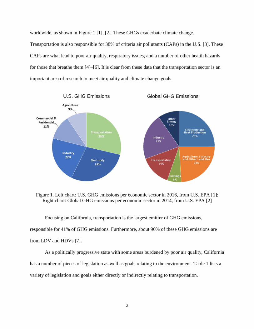
worldwide, as shown in Figure 1 [1], [2]. These GHGs exacerbate climate change.

Transportation is also responsible for 38% of criteria air pollutants (CAPs) in the U.S. [3]. These

CAPs are what lead to poor air quality, respiratory issues, and a number of other health hazards

for those that breathe them [4]–[6]. It is clear from these data that the transportation sector is an

important area of research to meet air quality and climate change goals.

Figure 1. Left chart: U.S. GHG emissions per economic sector in 2016, from U.S. EPA [1];

Right chart: Global GHG emissions per economic sector in 2014, from U.S. EPA [2]

Focusing on California, transportation is the largest emitter of GHG emissions,

responsible for 41% of GHG emissions. Furthermore, about 90% of these GHG emissions are

from LDV and HDVs [7].

As a politically progressive state with some areas burdened by poor air quality, California

has a number of pieces of legislation as well as goals relating to the environment. Table 1 lists a

variety of legislation and goals either directly or indirectly relating to transportation.

U.S. GHG Emissions Global GHG Emissions

3

Table 1. California transportation legislation and goals

Climate Change

AB 32: Global Warming Solutions

Act [8]

Reduce GHG emissions to 1990 amounts by 2020

SB 32: California Global Warming

Solutions act of 2006 [9]

Reduce GHG emissions to 40% below 1990 amounts by 2030

California Governor’s Executive

Order # S-03-05 [10]

Reduce GHG emissions to 80% below 1990 amounts by 2050

SB 2: Renewable Energy Resources

[11]

33% of electricity is renewable by 2020

SB 350: Clean Energy and Pollution

Reduction Act of 2015 [12]

50% of electricity is renewable by 2030

SB 100: California Renewables

Portfolio Standard Program [13]

100% of electricity is zero-carbon by 2045

SB 375: Sustainable Communities

[14]

Reduce GHG emissions by community planning for transportation and

land use

Transportation Fuel

Low Carbon Fuel Standards [15] Reduce carbon in transportation fuel by 10% in 2020

AB 1007: State Alternative Fuels

Plan [16]

Plan to use more alternative fuels in CA, including details on how to

increase hydrogen use

AB 118: California Alternative and

Renewable Fuel, Vehicle

Technology, Clean Air, and Carbon

Reduction Act [17]

Provides funding for technologies that improve local air quality

Zero Emissions Vehicle Action

Plan[18]

Plan to achieve 1.5 million ZEVs in CA by 2025

AB 8: Alternative Fuel and Vehicle

Technologies [19]

Allocates $20 million each year for hydrogen fueling stations until

100 are built

SB 1505: Environmental Standards

for Hydrogen Production [20]

Requires that hydrogen be 33.3% renewable, and have 30% lower

GHG and 50% lower CAP emissions than gasoline

Heavy-Duty Vehicles

AB 739: State vehicle fleet:

purchases [21]

A minimum of 15% of certain state-purchased heavy-duty vehicles

must be ZEVs by 2025 and 30% by 2030

AB 1073: California Clean Truck,

Bus, and Off-Road Vehicle and

Equipment Technology Program [22]

Extended funding for heavy-duty trucks, according to California’s

Clean Truck, Bus and Off-Road Vehicle program

Goods Movement Emission

Reduction Plan [23]

$1 billion allocated to a collaboration between California Air

Resources Board and local agencies to reduce pollutant emissions in

freight corridors

California Sustainable Freight Action

Plan [24]

Creates 2050 goals for cleaner freight system, targets for 2030, and

assistance in starting pilot projects

San Pedro Bay Ports Clean Air

Action Plan, 2018 Update [25]

Newly-registered trucks at the Ports of Long Beach and Los Angeles

must be model year 2014 or newer

4

Three key ideas are found in these goals and pieces of legislation: (1) California is

actively pursuing methods to reduce GHG and CAP emissions from both the electric grid and the

transportation sector, which are increasingly overlapping; (2) various fuels ranging from

electricity to hydrogen to others that are actively being researched are potential methods of these

emissions reductions; and (3) all classes of vehicles, including LDVs and HDVs, have room to

reduce emissions and support California’s efforts.

A study that analyzes the wide range of potential fuel pathways and powertrain

configurations for vehicles and optimizes an evolution of the transportation sector has yet to be

completed. Furthermore, there has not been a study that includes the breadth of vehicle fuels and

included a vehicle powertrain component of the optimization as well. This encompassing work,

however, is necessary due to the wide array of options. Simply analyzing a few of the fuels in

isolation from the powertrains, or a general analysis of the powertrains without including a

detailed study of the associated fuel pathways does not allow for a meaningful result that can

direct the evolution of the transportation sector at this critical time.

Both cost and emissions are two key components of these technologies. Cost is a

necessary consideration. If a technology has promising emissions reductions but is prohibitively

expensive, the technology will not be widely adopted due to economic constraints. Regarding

emissions, the aim is to combat climate change and improve air quality. Therefore, technologies

that reduce emissions and thereby allow for compliance with previously-introduced legislation

and goals should be prioritized. Therefore, a combined analysis of cost and emissions is needed

to better understand what technologies should be pursued.

This dissertation explores the future of the automobile, with emphasis on the fuels and

powertrains envisioned for alternative vehicles. With such a wide range of fuel pathways and

5

powertrain configurations, it is wise to establish an objective methodology to determine which

combination provides the most economical method of meeting our environmental goals.

Constructing a methodology that works for the bulk of the transportation sector, including LDVs

and HDVs, will yield the most insight and have the broadest impact on air quality and climate

change. While medium-duty vehicles (MDVs) are important to commerce, the GHG and CAP

emissions are relatively negligible when compared to the LDVs and HDVs modeled in the

present work.

1.2 Goal

The goal of this dissertation is to establish viable fuel pathways and powertrain

configurations for LDVs and HDVs that meet environmental constraints at the lowest cost. This

work develops a methodology to characterize and project various fuel pathways and powertrain

configurations techno-economic data and then determine a fleet to meet transportation needs into

2050. The results of this work will inform the transportation industry and policy makers how

society might effectively transform the transportation sector in a future of stricter environmental

regulations.

1.3 Objectives

To meet this dissertation goal, the following objectives will be completed:

1. Establish the fuel pathways for LDVs and HDVs.

2. Establish the powertrain configurations for LDVs and HDVs.

6

3. Develop efficiency, cost, and emissions data out to 2050 for the fuel pathways

established in Objective 1 and the vehicle powertrain configurations established in

Objective 2.

4. Establish the constraints of the optimization problem using California legislation and

executive order for emissions, realistic growth scenarios for travel and technology, and

feedstock availability.

5. Determine optimization tool to use given the results of Objectives 3 and 4, and establish

the formal optimization problem.

6. Solve the optimization problem established in Objective 5 to determine the emissions and

cost impacts of the optimum cases. Compare these results to the Reference Case.

7. Systematically assess the results to establish viable fuel pathways and powertrain

configurations for LDVs and HDVs that meet the constraints of this problem.

7

2. BACKGROUND

Areas of study that are relevant to this work include vehicle fuel production methods,

vehicle powertrain configurations, and optimization techniques. Each of these three areas will be

discussed in the following sections in as much detail as is needed to follow the work of this

dissertation.

The scope of analysis for this work is known as well-to-wheels (WTW). This includes the

production of fuel from its feedstock, the distribution of the fuel, the dispensing of the fuel, and

the use of the fuel in vehicles.

2.1 Vehicle Fuels

Five alternative fuels are likely to be used in the next few decades in LDVs and HDVs.

These fuels are electricity, hydrogen, substitute natural gas (SNG), renewable gasoline, and

renewable diesel [26]–[30].

Each of the above fuels can be produced in a variety of manners. Some constraint on the

scope of this work is used to focus on pathways that are, according to the state of the art of this

writing, more likely to be viable from cost and efficiency perspectives. This does not preclude

the fact that future technology advancements may introduce new fuels or pathways. It is

important to note that while these potential future advancements could mean reality may be

different from the projections of the present work, the advancements can be integrated into the

methodology introduced herein at the time that they are discovered. It is recommended that the

current state of the art be updated from time to time to ensure the most accurate data are used.

8

2.1.1 Fuel Feedstocks

A fuel feedstock is an input that is converted to a fuel through one of a multitude of fuel

production technologies that are available. For the five alternative fuels introduced, there are two

broad feedstock categories: electricity and biomass.

2.1.1.1 Electricity

Electricity is widely familiar throughout society as a means of turning on lights, running

fans, charging phones, and many other daily necessities of the modern world. Less familiar to

most is using electricity as a main input for making vehicle fuels. Most would understand how

electricity might be used in various processes of refining gasoline for cars. However, for some

alternative fuels for vehicles, electricity is a main feedstock. Furthermore, certain kinds of

vehicles, known as plug-in electric vehicles (PEVs), use electricity directly as a fuel.

As a fuel feedstock, electricity is primarily used to convert water into hydrogen in a

process known as electrolysis. Water could be considered a co-feedstock along with electricity.

However, given the techno-economic nature of this work, and the fact that water costs will likely

stay a small fraction of overall fuel costs, which will be discussed in more detail later in this

dissertation, the water feedstock is not further considered in this work. It should be noted,

however, that future electrolytic fuel production should be located in an area with water

availability to increase efficiency and cost-effectiveness.

9

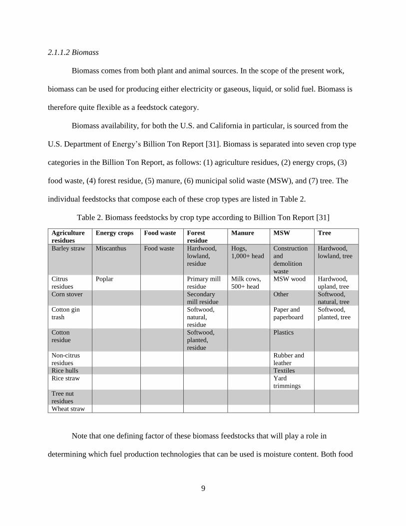
2.1.1.2 Biomass

Biomass comes from both plant and animal sources. In the scope of the present work,

biomass can be used for producing either electricity or gaseous, liquid, or solid fuel. Biomass is

therefore quite flexible as a feedstock category.

Biomass availability, for both the U.S. and California in particular, is sourced from the

U.S. Department of Energy’s Billion Ton Report [31]. Biomass is separated into seven crop type

categories in the Billion Ton Report, as follows: (1) agriculture residues, (2) energy crops, (3)

food waste, (4) forest residue, (5) manure, (6) municipal solid waste (MSW), and (7) tree. The

individual feedstocks that compose each of these crop types are listed in Table 2.

Table 2. Biomass feedstocks by crop type according to Billion Ton Report [31]

Agriculture

residues

Energy crops Food waste Forest

residue

Manure MSW Tree

Barley straw Miscanthus Food waste Hardwood,

lowland,

residue

Hogs,

1,000+ head

Construction

and

demolition

waste

Hardwood,

lowland, tree

Citrus

residues

Poplar Primary mill

residue

Milk cows,

500+ head

MSW wood Hardwood,

upland, tree

Corn stover Secondary

mill residue

Other Softwood,

natural, tree

Cotton gin

trash

Softwood,

natural,

residue

Paper and

paperboard

Softwood,

planted, tree

Cotton

residue

Softwood,

planted,

residue

Plastics

Non-citrus

residues

Rubber and

leather

Rice hulls Textiles

Rice straw Yard

trimmings

Tree nut

residues

Wheat straw

Note that one defining factor of these biomass feedstocks that will play a role in

determining which fuel production technologies that can be used is moisture content. Both food

10

waste and manure categories are high-moisture biomass categories, whereas the rest are typically

dry.

Additionally, the non-organic portions of the MSW, which include plastics, rubber, and

leather, are not included in this analysis as potential fuel production feedstocks. The feedstock

quantities that will later be shown reflect this removal of the non-organic MSW from the original

Billion Ton Report data.

2.1.2 Fuel Production

What follows are descriptions of the various methods of fuel productions for the five

fuels considered in this work, categorized first by the fuel being produced and then by the

specific fuel production technology adopted.

2.1.2.1 Electricity Production

From the perspective of PEVs, electricity is the fuel itself, and not simply a feedstock as

introduced previously. This work assumes the electricity production feedstocks and methods as

projected by entities such as Energy and Environmental Economics (E3) [32] and Argonne

National Laboratory’s GREET Model [33]. The reasoning for this is that the electricity sector is

larger than simply the demand for transportation. There are legislation and goals for the electric

grid in particular, and therefore it is reasonable to assume that a transportation analysis will not

dramatically impact the evolution of the feedstock portfolio for electricity generation. However,

it is important to note that transportation and electricity generation are increasingly intertwined

as vehicle electrification increases.

11

Electricity is generated from a wide variety of sources, ranging from fossil fuels such as

natural gas used in gas turbines to renewable sources such as solar panels. Due to the wide

variation in the production of electricity that is beyond the scope of this work, the PATHWAYS

model by E3 is used to determine how the electricity grid composition will change with time

[32]. This model shows the projected evolution of the electric grid from 2015 to 2050 along

various evolution scenarios. The one used for this dissertation is the “Straight Line” scenario

which assumes a linear reduction in emissions to reach emissions reductions goals in 2050, and

also complies with the recent SB 100 legislation that was introduced in Table 1.

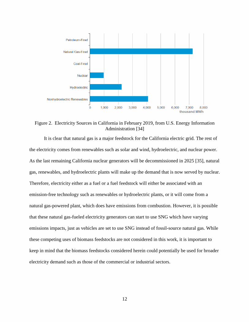
Detailed electricity production discussion is outside the scope of this work for the reasons

stated above. However, some general facts are important to note. Figure 2 displays the electricity

generation sources in California for February 2019 with data from the U.S. Energy Information

Administration [34]. Natural gas is used in combustion electricity generators known as gas

turbines. There are various evolutions of the gas turbine plant, including combined cycle plants

which use waste heat of the gas turbine as heat input for a steam turbine to produce additional

electricity from the same natural gas fuel input. Nuclear power, while somewhat significant in

terms of power generated, is set to be phased out of California when the last nuclear plant at

Diablo Canyon is shut down in 2025 [35]. Coal has been almost completely phased out, with

only one plant still producing electricity from coal [36], and it is unlikely to return due to the

strict environmental regulations of the State.

12

Figure 2. Electricity Sources in California in February 2019, from U.S. Energy Information

Administration [34]

It is clear that natural gas is a major feedstock for the California electric grid. The rest of

the electricity comes from renewables such as solar and wind, hydroelectric, and nuclear power.

As the last remaining California nuclear generators will be decommissioned in 2025 [35], natural

gas, renewables, and hydroelectric plants will make up the demand that is now served by nuclear.

Therefore, electricity either as a fuel or a fuel feedstock will either be associated with an

emission-free technology such as renewables or hydroelectric plants, or it will come from a

natural gas-powered plant, which does have emissions from combustion. However, it is possible

that these natural gas-fueled electricity generators can start to use SNG which have varying

emissions impacts, just as vehicles are set to use SNG instead of fossil-source natural gas. While

these competing uses of biomass feedstocks are not considered in this work, it is important to

keep in mind that the biomass feedstocks considered herein could potentially be used for broader

electricity demand such as those of the commercial or industrial sectors.

13

2.1.2.2 Hydrogen Production

Hydrogen is a gaseous fuel at ambient temperature and pressure, though it is often stored

at higher pressures to increase volumetric energy density. Hydrogen can be combusted like

current fossil fuels in vehicles, but in this work it is assumed that hydrogen is a fuel only for fuel

cells. Fuel cells are electrochemical conversion devices, and more detailed information about

them will come later in the section discussing the various vehicle powertrain configurations.

Suffice it to say for now that fuel cells are an alternative to combustion engines which do not

have any harmful emissions when fueled by hydrogen.

Hydrogen can be made from one of three major production methods. First, hydrogen can

be produced from electrolysis of water, meaning production efficiency and associated emissions

are heavily dependent on those of the electricity used. Second, hydrogen can also be produced

from biomass gasification. Gasification involves heating dried biomass without an oxidant (air)

to produce bio-oils, a process known as pyrolysis. Next, the bio-oils are further heated with an

oxidant (such as air) and water. Fuels produced from biomass feedstocks, such as hydrogen from

biomass gasification, are known as biofuels. Thirdly, hydrogen can be produced from steam

methane reformation (SMR). SMR is a process in which methane and water react at high

temperatures to produce hydrogen. The methane being reformed can come from one of the SNG

processes described in the relevant section of this dissertation.

a) Electrolytic Hydrogen Production

Electrolysis splits water with electricity to produce hydrogen and oxygen using

electrolyzers of three main varieties: alkaline electrolytic cells (AECs), proton exchange

membrane electrolytic cells (PEMECs), and solid oxide electrolytic cells (SOECs). AECs are the

14

most mature form of electrolyzers of these three in that they have been available commercially

for the longest time. PEMECs are the next most mature. SOECs are the least mature electrolyzer,

with no commercially available examples available and a technology readiness level (TRL) of 2-

4 in 2014 [37].

Power-to-gas (P2G) is an emerging technology that transforms energy in the form of

electricity to energy in the form of a gaseous fuel such as hydrogen (or methane, which will be

detailed shortly). This is useful due to the increasing amount of renewable energy such as wind

and solar which are intermittent and not easily predictable. P2G can be used as a form of energy

storage in that the gas that is produced from electricity can be stored in containers or even the

natural gas grid for later use either as a vehicle fuel or fuel for other purposes.

P2G is flexible due to the numerous possible pathways for energy to flow. These

pathways are depicted in Figure 3. P2G can connect the electric grid and the natural gas grid, two

large energy distributors of the modern day. This allows the benefits of both grids to be utilized

while downplaying their characteristic issues. For example, P2G can use the highly efficient

electric grid when possible (meaning there is demand for more electricity), but also use the

natural gas grid when there is not an immediate demand for power (making use of the natural gas

grid’s inherent storage ability). P2G also enables other transfers of energy, such as fueling

vehicles that run on hydrogen, natural gas, or electricity.

15

Figure 3. Schematic of P2G Pathways, from the Advanced Power and Energy Program [38]

As seen from Figure 3, the first step in P2G, no matter which pathway is being followed,

is using electricity in an electrolyzer to produce hydrogen. Therefore, the emissions associated

with P2G are directly tied to the emissions associated with the production of the electricity used

by the electrolyzer. While Figure 3 only shows renewable sources of electricity, P2G can also

use fossil sources of electricity which do have emissions.

A particularly attractive use of P2G comes from using what would be curtailed, or

wasted, electricity from renewable energy sources such as solar panels and wind turbines [39].

As mentioned above, both wind and solar power are intermittent and hard to predict precisely.

P2G is able to use electricity from these renewable sources at times when the electric grid might

not be able to accept them, which is brought about by the fact that electricity must continually be

used at the same time as it is generated. This means more of the renewable electricity generated

would be used in other areas such as making renewable hydrogen for vehicle fuel. Increasing

renewable energy usage will decrease the emissions associated with both the electric grid and the

natural gas grid, which are both intertwined with the advent of P2G.

16

To focus on the work conducted within this dissertation, it is beneficial to summarize the

pathways and technologies used herein. Figure 4 is a flowchart that includes all such pathways

for electrolytic hydrogen production. The overall idea of these pathways is to use electricity

(produced from either fossil fuels or non-fossil fuels such as solar and wind power) to produce

hydrogen from water. This gaseous fuel can be made by any of the three electrolyzer

technologies displayed below.

Figure 4. Flowchart of analyzed electrolytic hydrogen production pathways

b) Gasification Hydrogen Production

Gasification is a thermochemical process in which solid biomass is heated in the absence

of oxygen to produce a gaseous mixture known as syngas [40]. This syngas is composed

primarily of hydrogen and carbon monoxide. Hydrogen can then be separated from this mixture

[41][42][43], [44][45]–[52].

Note that gasification is most efficient with dry biomass [40]. Drying would be required

for higher moisture content biomass, and the efficiency loss there would make gasification less

attractive than an alternative process such as anaerobic digestion, which will be introduced later.

17

Therefore, this work assumes only dry biomass as potential feedstocks for gasification, including

agricultural residues, MSW, forestry residues, trees, and energy crops. Food waste and manure

are not considered feedstocks for gasification in this work as they would require significant

drying which would decrease overall efficiency.

c) Steam Methane Reformation Hydrogen Production

SMR is a chemical reaction in which methane (CH4) is converted to hydrogen (H2)

according to the following reaction in Equation 1.

Equation 1. Steam methane reformation reaction

CH4 + H2O → CO2 + 4H2

This process is currently used on natural gas, a fossil fuel, to make 95% of hydrogen in

the U.S. [53]. Additionally, some biogas is put through SMR to meet SB 1505, the requirement

that one-third of hydrogen sold at fueling stations is renewable.

Due to this work’s focus on increasing adoption of renewable fuels and the roundabout

method of production using SMR which lowers efficiency by about 70% [54] (first biogas would

need to be produced from the primary biomass by one of the methods to be introduced shortly,

and then that biogas would be converted to hydrogen), this production method is not considered

in this work.

2.1.2.3 SNG Production

Substitute natural gas (SNG) is a drop-in fuel, meaning it can be integrated into current

natural gas infrastructure, including pipelines and dispensing stations, and be used in current

vehicles that are fueled by natural gas. Being a drop-in fuel allows for easy integration of a fuel

that can be made in a more environmentally-friendly manner, and using resources that may be

18

more prevalent in any given area. One potential benefit of drop-in fuels such as SNG is time of

transition: it may take less time to reduce emissions by changing the fuel than by changing the

vehicle, either with efficiency improvements or alternative powertrain technologies.

Three methods of producing SNG are considered in this dissertation. Those three

methods are electrolytic methanation and biomass conversion by either anaerobic digestion or

gasification. Electrolytic production of SNG uses electricity as its feedstock. This process begins

the same as electrolytic hydrogen production, and is followed by a methanation step to convert

that hydrogen into methane using carbon dioxide. Anaerobic digestion (AD) is a biochemical

process that uses microbes to break down organic matter to methane and carbon dioxide.

Gasification for SNG production, as for hydrogen mentioned previously, requires lower moisture

biomass. Again, these dry biomass feedstocks are agricultural residues, MSW, forestry residues,

trees, and energy crops.

a) Electrolytic SNG Production

Electrolytic methanation starts in the same way as electrolytic hydrogen, but there is a

following methanation step. This production method also belongs to the umbrella term P2G

introduced previously.

Methanation is the chemical reaction that turns hydrogen and carbon dioxide into

methane and water. This chemical reaction is also known as the Sabatier reaction, and it is

exothermic, meaning heat is a product. The chemical equation is listed below with the correct

stoichiometric coefficients in Equation 2. Each mole of reaction gives off 165 kilojoules of heat

[55].

19

Equation 2. Sabatier reaction

𝐶𝑂2 + 4𝐻2 → 𝐶𝐻4 + 2𝐻2𝑂

Literature was consulted for technologies that provide carbon dioxide for making SNG

from hydrogen as well as technologies to make use of the heat produced during the methanation

process. Both of these technologies are needed because the Sabatier reaction (1) is an exothermic

reaction that requires a heat sink for sustained reaction without overheating equipment, and (2)

requires carbon dioxide as input to convert hydrogen into methane [56].

The primary benefit of methanation is the ability to take advantage of the natural gas

infrastructure. Without methanation, hydrogen is the main product of P2G. However, there is not

much infrastructure in the U.S., or even the world, for hydrogen. Therefore, the extra step of

methanation makes P2G much simpler to integrate into the power grid of today and transport to

areas of demand. Use of natural gas pipelines and storage throughout the country and much of

the rest of the world make P2G more practical today. The tradeoff for this practicality is the loss

of efficiency by adding the extra step of methanation as well as the additional emission of carbon

wherever the SNG is eventually used.

Because methanation can take place at a range of temperatures and its efficiency is

benefitted by some pressurization, it is wise to include a range of temperatures and an above-

ambient pressure in calculations [55]. An equilibrium analysis using NASA’s Chemical

Equilibrium with Applications code at 5 atmospheres of pressure at 400, 500, and 600oC leads to

an average methanation efficiency of 0.7904 [57]–[59]. This is calculated by analyzing the

products of the Sabatier reaction at the given pressure and temperatures, and determining what

fraction of the products is methane, the desired product.

20

Methanation is pressure dependent in such a way that it is more efficient at producing

methane at higher pressures [60]. Methanation efficiency is highly dependent on reaction

temperature. At 400oC with a 4 to 1 molar ratio of hydrogen to methane input (the stoichiometric

ratio of the Sabatier reaction), the methanator output is 92% methane; at 500oC, the output is

81% methane; and at 600oC, the output is 64% methane. Therefore, operating at a lower

temperature would increase the amount of methane coming out of the methanator, which could

also remove the need for any gas cleanup before injection into the natural gas pipeline. However,

it is important to keep in mind other effects of lowering the temperature of the methanator. One

major impact is there will be lower quality waste heat which would be used in other P2G

processes to be expanded upon later. This could lower the overall process efficiency, even if the

amount of methane is decreased. A more careful analysis would be needed based upon an

individual plant design.

See Figure 5 for equilibrium species concentration of a methanator at 5 atmospheres of

pressure. Note that some methanators may not allow for the full expected conversion of carbon

dioxide and hydrogen to methane due to time reacting. Because the calculations discussed are for

equilibrium concentrations, and equilibrium takes time to achieve, actual methanation efficiency

may be lower than calculated if time spent reacting in the methanator does not allow for

equilibrium to be reached. Therefore, it is important to ensure reactor design does so, or account

for the drop in conversion efficiency of the methanator used.

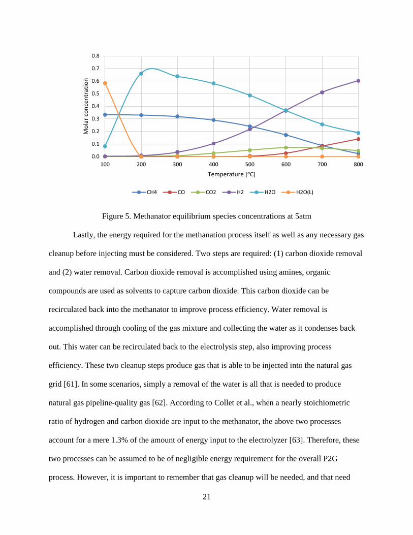
21

Figure 5. Methanator equilibrium species concentrations at 5atm

Lastly, the energy required for the methanation process itself as well as any necessary gas

cleanup before injecting must be considered. Two steps are required: (1) carbon dioxide removal

and (2) water removal. Carbon dioxide removal is accomplished using amines, organic

compounds are used as solvents to capture carbon dioxide. This carbon dioxide can be

recirculated back into the methanator to improve process efficiency. Water removal is

accomplished through cooling of the gas mixture and collecting the water as it condenses back

out. This water can be recirculated back to the electrolysis step, also improving process

efficiency. These two cleanup steps produce gas that is able to be injected into the natural gas

grid [61]. In some scenarios, simply a removal of the water is all that is needed to produce

natural gas pipeline-quality gas [62]. According to Collet et al., when a nearly stoichiometric

ratio of hydrogen and carbon dioxide are input to the methanator, the above two processes

account for a mere 1.3% of the amount of energy input to the electrolyzer [63]. Therefore, these

two processes can be assumed to be of negligible energy requirement for the overall P2G

process. However, it is important to remember that gas cleanup will be needed, and that need

0.0

0.1

0.2

0.3

0.4

0.5

0.6

0.7

0.8

100 200 300 400 500 600 700 800

Mo

lar

con

cen

trat

ion

Temperature [oC]

CH4 CO CO2 H2 H2O H2O(L)

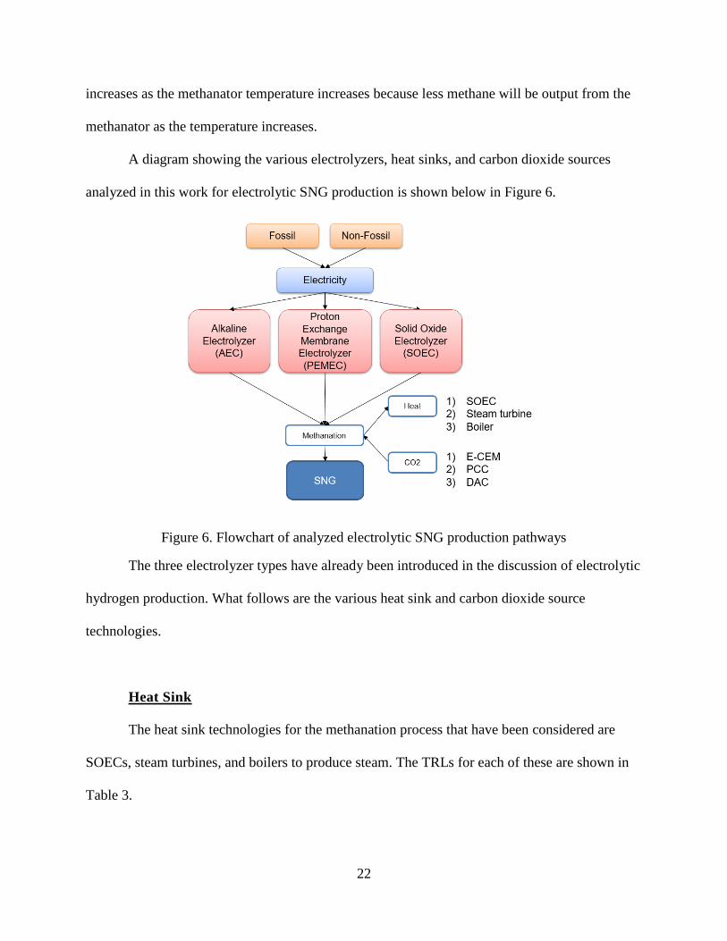
22

increases as the methanator temperature increases because less methane will be output from the

methanator as the temperature increases.

A diagram showing the various electrolyzers, heat sinks, and carbon dioxide sources

analyzed in this work for electrolytic SNG production is shown below in Figure 6.

Figure 6. Flowchart of analyzed electrolytic SNG production pathways

The three electrolyzer types have already been introduced in the discussion of electrolytic

hydrogen production. What follows are the various heat sink and carbon dioxide source

technologies.

Heat Sink

The heat sink technologies for the methanation process that have been considered are

SOECs, steam turbines, and boilers to produce steam. The TRLs for each of these are shown in

Table 3.

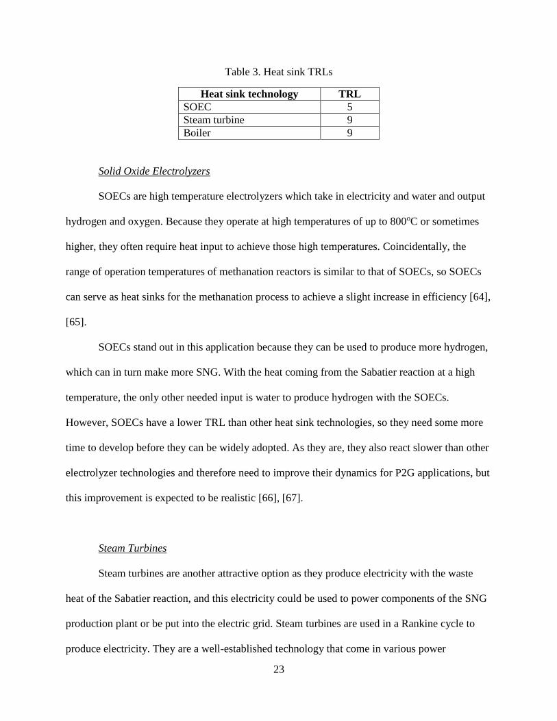
23

Table 3. Heat sink TRLs

Heat sink technology TRL

SOEC 5

Steam turbine 9

Boiler 9

Solid Oxide Electrolyzers

SOECs are high temperature electrolyzers which take in electricity and water and output

hydrogen and oxygen. Because they operate at high temperatures of up to 800oC or sometimes

higher, they often require heat input to achieve those high temperatures. Coincidentally, the

range of operation temperatures of methanation reactors is similar to that of SOECs, so SOECs

can serve as heat sinks for the methanation process to achieve a slight increase in efficiency [64],

[65].

SOECs stand out in this application because they can be used to produce more hydrogen,

which can in turn make more SNG. With the heat coming from the Sabatier reaction at a high

temperature, the only other needed input is water to produce hydrogen with the SOECs.

However, SOECs have a lower TRL than other heat sink technologies, so they need some more

time to develop before they can be widely adopted. As they are, they also react slower than other

electrolyzer technologies and therefore need to improve their dynamics for P2G applications, but

this improvement is expected to be realistic [66], [67].

Steam Turbines

Steam turbines are another attractive option as they produce electricity with the waste

heat of the Sabatier reaction, and this electricity could be used to power components of the SNG

production plant or be put into the electric grid. Steam turbines are used in a Rankine cycle to

produce electricity. They are a well-established technology that come in various power

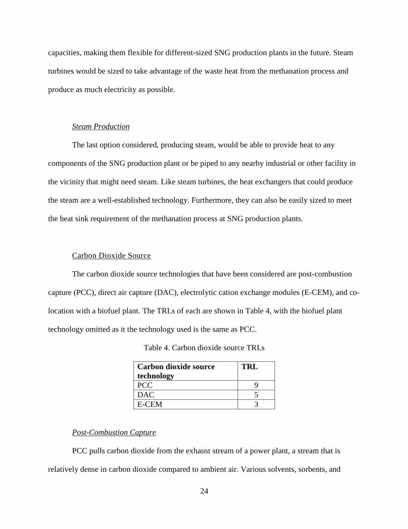
24

capacities, making them flexible for different-sized SNG production plants in the future. Steam

turbines would be sized to take advantage of the waste heat from the methanation process and

produce as much electricity as possible.

Steam Production

The last option considered, producing steam, would be able to provide heat to any

components of the SNG production plant or be piped to any nearby industrial or other facility in

the vicinity that might need steam. Like steam turbines, the heat exchangers that could produce

the steam are a well-established technology. Furthermore, they can also be easily sized to meet

the heat sink requirement of the methanation process at SNG production plants.

Carbon Dioxide Source

The carbon dioxide source technologies that have been considered are post-combustion

capture (PCC), direct air capture (DAC), electrolytic cation exchange modules (E-CEM), and co-

location with a biofuel plant. The TRLs of each are shown in Table 4, with the biofuel plant

technology omitted as it the technology used is the same as PCC.

Table 4. Carbon dioxide source TRLs

Carbon dioxide source

technology

TRL

PCC 9

DAC 5

E-CEM 3

Post-Combustion Capture

PCC pulls carbon dioxide from the exhaust stream of a power plant, a stream that is

relatively dense in carbon dioxide compared to ambient air. Various solvents, sorbents, and

25

membranes are used to capture the carbon dioxide from the exhaust stream as the carbon

dioxide-containing exhaust flows through the PCC system. Solvents and sorbents capture carbon

dioxide and release it under certain conditions such as heating or compressing. Membranes allow

only specific molecules, such as carbon dioxide in the case of PCC, to pass through, and other

molecules are blocked from passing [68], [69].

The relatively high concentration of carbon dioxide in the exhaust stream of a power

plant makes capturing carbon more efficient compared to a less-concentrated source such as

ambient air. Priority should be given to the largest sources of carbon dioxide, such as very large

power plants, so these PCC installations can capture the most emissions with the least effort of

installing systems.

One consideration for PCC placement is the effect on nearby ecosystems due to the

decreased carbon dioxide in the air. Particularly for vegetation downstream of the exhaust, the

drastic decrease in carbon dioxide can affect growth, which may have undesired effects on the

ecosystem as a whole [70]. Of course, the amount of carbon dioxide emitted worldwide must be

reduced; the preceding comment is included just to make the reader aware of potential side-

effects of the technologies studied herein.

Direct Air Capture

DAC also involves a sorbent to capture carbon dioxide from the ambient air [70].

Because of the lower density of carbon dioxide in ambient air compared to the exhaust stream of

a power plant, DAC is not as efficient as PCC.

Due to the nature of carbon dioxide’s effect on climate change, DAC units can be placed

anywhere and have the same impact. A given amount of carbon dioxide captured has the same

26

effect on climate change no matter where that carbon dioxide is captured. However, it would be

wise to place the DAC units in places with cheap and clean power to make operation more

economical and more beneficial to the environment. Additionally, ambient air characteristics

affect performance of the DAC systems, so placement should be done based on careful analysis.

Humidity has a significant effect on performance due to the water molecules’ interference with

carbon dioxide capture. Similarly, other molecules in the air such as pollution can effect carbon

dioxide capture by either their physical presence or chemical reactions with parts of the DAC

system [70].

Similar to that which was discussed for PCC, a further consideration for DAC is the

effect it has on ecosystems. Because DACs take in ambient air, the concentration of carbon

dioxide is lower than in the exhaust for power plants. Therefore, DAC has the potential to

deplete carbon dioxide to a level that could affect downstream ecosystems [70]. And again,

carbon dioxide levels should be reduced; this is simply a side-effect that should be considered.

Electrolytic Cation Exchange Module

E-CEM technology is being pursued by the U.S. Navy and is promising due to its ability

to capture both carbon dioxide and hydrogen from seawater [71]. Here, the carbon dioxide would

be used as an input to the Sabatier reaction, and the hydrogen again is useful as a fuel or as more

reactant for the Sabatier reaction. E-CEM was originally developed for jet fuel production in the

sea to overcome the need for resupply of fuel on military missions involving aircraft carriers.

However, the basic technology can be adapted to P2G by removing the final fuel synthesis step

and instead stopping with carbon dioxide and hydrogen as the desired products, which are

exactly what are needed for the methanation reaction.

27

The process is powered by ocean thermal energy conversion (OTEC), which uses the

temperature difference in water at different depths. While circulating through the OTEC process,

small amounts of the carbon in water, in the form of dissolved carbon dioxide, can be captured.

Further carbon dioxide can be captured from the carbonates in seawater with additional capture

materials and power from OTEC. Hydrogen is produced by PEMEC or AEC technology, using

the electricity produced by OTEC [72]. While not mentioned in the report, SOEC technology

could be used for hydrogen production as well.

The technology readiness level for E-CEM is low and therefore the option may not be

ready in time for use in 2030 or 2050.

Co-location of Electrolytic SNG Production with Biofuel Plants

A fourth source of carbon dioxide is from biofuel plants. These biofuel plants produce

carbon dioxide which can be captured with some additional plant equipment [73]. Biorefineries

such as those producing biofuels from AD, pyrolysis, hydrolysis, and gasification have streams

with relatively high concentrations of carbon dioxide [74]–[80]. The carbon dioxide can be

separated from the streams rather efficiently, typically using differences in condensing

temperatures of the stream constituents or any of the various methods used by PCC and DAC

technologies. Note that this separation technology is effectively the same as that of PCC

mentioned previously. Each of the above mentioned production methods will have different

concentrations of carbon dioxide in various streams, so the efficiency and quantity of carbon

dioxide will be different for each. However, there is an expected synergy of co-locating a P2G

plant with a biorefinery due to the much higher concentration of carbon dioxide in the stream so

of the biorefinery compared to the ambient air (in the case of a DAC) and the seawater (in the

28

case of E-CEM). This is similar to the high carbon dioxide concentration utilized in PCC, but

biorefineries have the added benefit of using biomass as input, drastically improving the carbon

impact of these facilities.

This concept is particularly attractive in situations in which the biofuel processing plants

are co-located with electrolysis plants with solar or wind power on-site. The coalescing of these

pieces of equipment create a synergy of fuel production, of both the original fuel of the biofuel

plant and the electrolytic SNG. The main benefit of this layout is to take advantage of low

electricity costs due to on-site renewable generation and the otherwise-wasted carbon dioxide

from the biomass at a low marginal cost.

b) Anaerobic Digestion SNG Production

SNG can also be produced using a biochemical process known as anaerobic digestion.

Anaerobic digestion involves microbes (hence biochemical), in the absence of oxygen, breaking

down organic matter to methane and carbon dioxide. This process works with high moisture

biomass, so only the moist biomass sources including manure and food waste can be used in AD

[81]–[84]. One could co-digest a lower-moisture content biomass feedstock such as a somewhat

moist agriculture waste (for example, fresh yard trimmings). This would require the feedstocks

be added in such a ratio as the overall slurry has a high enough moisture content to work in the

AD [83]. The work of this dissertation is not spatially resolved, so this constraint is not able to be

considered. Given the fact that this co-digestion is rare in the literature, this simplification should

not have much impact on practical results. Therefore, only manure and food waste will be

considered feedstocks for anaerobic digestion.

29

The gas mixture of mostly methane and carbon dioxide can be cleaned to improve the

purity of methane using methods previous introduced, creating SNG. The wet material remaining

after AD, known as digestate, can be used as a fertilizer for farming applications [85].

c) Gasification SNG Production

Gasification was previously introduced as a method of producing hydrogen from dry

biomass. Again, the actual product of gasification is termed syngas, which is composed primarily

of hydrogen and carbon monoxide. This syngas can be turned into SNG by the same methanation

process described previously to convert electrolytic hydrogen and carbon dioxide into methane

[86], [87], [96]–[104], [88]–[95][105], [106], [115], [116], [107]–[114].

Just as before with hydrogen gasification, producing SNG by gasification is also most

appropriate with a relatively dry biomass, which saves energy on the drying process. Therefore,

this work assumes only dry biomass as potential feedstocks for gasification, including

agricultural residues, MSW, forestry residues, trees, and energy crops. Food waste and manure

are not considered feedstocks for gasification in this work as they would require significant

drying which would decrease overall efficiency.

2.1.2.4 Renewable Gasoline and Renewable Diesel Production

Renewable gasoline and renewable diesel are both drop-in fuels, just as SNG is.

Therefore, these liquid fuels can be used in the current gasoline and diesel infrastructure,

including the many dispensing stations open today, as well as the vehicles that are fueled by

gasoline and diesel. Taking advantage of the vast incumbent gasoline and diesel infrastructure

30

and vehicles provides a significant timing and cost benefit to the renewable gasoline and

renewable diesel.

Renewable gasoline and diesel can both be produced from biomass using one of four

processes: liquefaction, gasification followed by Fischer-Tropsch, pyrolysis, and hydrolysis. The

three former production methods are thermochemical, whereas hydrolysis is biochemical. These

production methods will be discussed in further detail shortly. The differentiation between

renewable gasoline and diesel comes about through the refining process, similar to how fossil

gasoline and fossil diesel are differentiated from crude fossil oil. There are no distinctions made

for the different biomass feedstocks when producing either renewable gasoline or diesel. Also

important to note is that each of these four fuel production methods use the nearly the same

biomass feedstocks, which are relatively dry: agriculture, waste, forestry, tree, and energy crops.

However, liquefaction can also use moist biomass, so food waste and manure are included as

feedstocks for liquefaction [81], [117]–[119].

a) Liquefaction Renewable Gasoline and Renewable Diesel Production

Liquefaction is a direct conversion from biomass to liquid oils, and it is not as

technologically developed as some of the other liquid fuels production methods that will be

discussed. It involves heating and pressurizing biomass without oxidant at roughly 250-325oC

and 50-200 atmospheres of pressure. The result is a bio-oil which is then treated and refined to

produce the desired hydrocarbon, either renewable gasoline or renewable diesel. The treatment

process involves removing oxygen through hydrotreating, creating hydrocarbon chains of

desirable length through hydrocracking, and then distilling to get the desired spectrum of

hydrocarbons [81], [117]–[119][120][121]. In this work, the desired product is gasoline or diesel,

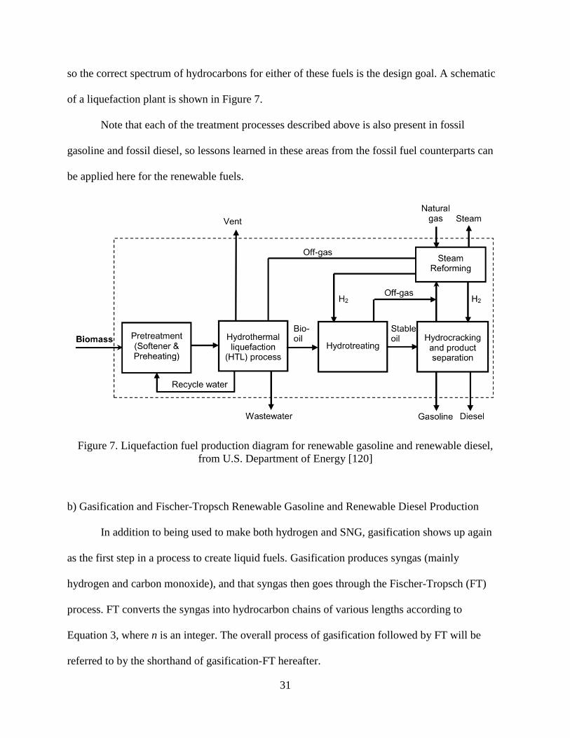
31

so the correct spectrum of hydrocarbons for either of these fuels is the design goal. A schematic

of a liquefaction plant is shown in Figure 7.

Note that each of the treatment processes described above is also present in fossil

gasoline and fossil diesel, so lessons learned in these areas from the fossil fuel counterparts can

be applied here for the renewable fuels.

Figure 7. Liquefaction fuel production diagram for renewable gasoline and renewable diesel,

from U.S. Department of Energy [120]

b) Gasification and Fischer-Tropsch Renewable Gasoline and Renewable Diesel Production

In addition to being used to make both hydrogen and SNG, gasification shows up again

as the first step in a process to create liquid fuels. Gasification produces syngas (mainly

hydrogen and carbon monoxide), and that syngas then goes through the Fischer-Tropsch (FT)

process. FT converts the syngas into hydrocarbon chains of various lengths according to

Equation 3, where n is an integer. The overall process of gasification followed by FT will be

referred to by the shorthand of gasification-FT hereafter.

32

Equation 3. Fischer-Tropsch process, from [122]

(2n + 1)H2 + n CO → CnH2n+2 + n H2O

This process uses a catalyst to produce the hydrocarbon products. As before in

liquefaction, the resulting products are hydrotreated, hydrocracked, and distilled for the final

desired products of either renewable gasoline or diesel. See Figure 8 for a flow diagram of the

gasification and Fischer-Tropsch process.

Figure 8. Gasification and Fischer-Tropsch production diagram for renewable gasoline and

diesel, from U.S. Department of Energy [122]

c) Pyrolysis Renewable Gasoline and Renewable Diesel Production

In pyrolysis, the dried biomass is pressurized to 1 to 5 atmospheres and heated up to 300-

500oC without an oxidant to produce bio-oils which are then refined to produce either gasoline or

diesel. Once again, the resultant bio-oil is hydrotreated, hydrocracked, and distilled to produce

either renewable gasoline or diesel [81], [117]–[119].

33

d) Hydrolysis Renewable Gasoline and Renewable Diesel Production

In hydrolysis, the cellulose of biomass (a structural component of plant cell walls) is

broken down by enzymes and water to produce hydrocarbons. These hydrocarbons can then be

processed through the same hydrotreating, hydrocracking, and distilling to obtain renewable

gasoline or diesel. Like gasification, hydrolysis is relatively early in its development state.

Unlike the other production methods, hydrolysis is a biochemical process due to the enzymes

that convert the biomass [81], [117]–[119].

2.1.2.5 Summary of Fuel Production Pathways

Having finished the introduction of each of the fuel pathways to be considered in this

work, Figure 9 summarizes them. Note the many pathways options, particularly with respect to

some of the biomass feedstocks that have several process options available. This diagram

highlights the need for an objective methodology of determining which pathways should be

pursued to fuel transportation needs into the future.

34

Figure 9. Flow diagram of fuel production pathways

2.1.3 Fuel Distribution

Once the fuels have been produced, it is then necessary to distribute them to locations at

which drivers can refuel their vehicles. Due to the physical differences between these fuels, there

are also major differences in how these fuels may be distributed.

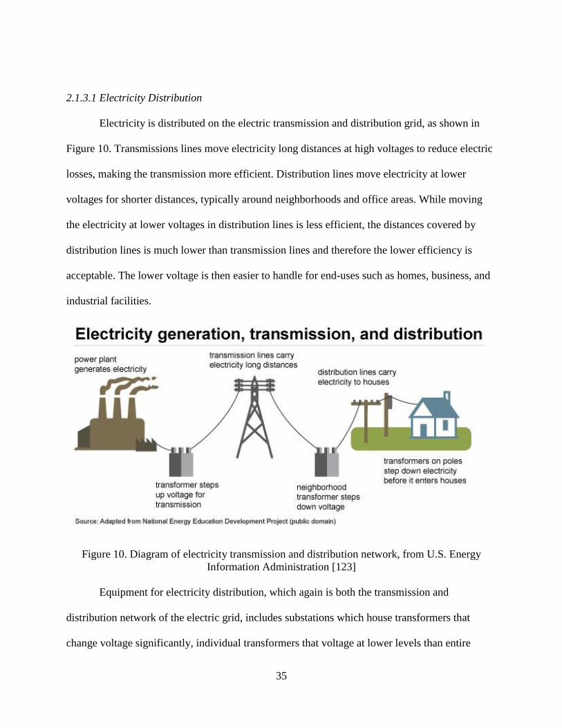
35

2.1.3.1 Electricity Distribution

Electricity is distributed on the electric transmission and distribution grid, as shown in

Figure 10. Transmissions lines move electricity long distances at high voltages to reduce electric

losses, making the transmission more efficient. Distribution lines move electricity at lower

voltages for shorter distances, typically around neighborhoods and office areas. While moving

the electricity at lower voltages in distribution lines is less efficient, the distances covered by

distribution lines is much lower than transmission lines and therefore the lower efficiency is

acceptable. The lower voltage is then easier to handle for end-uses such as homes, business, and

industrial facilities.

Figure 10. Diagram of electricity transmission and distribution network, from U.S. Energy

Information Administration [123]

Equipment for electricity distribution, which again is both the transmission and

distribution network of the electric grid, includes substations which house transformers that

change voltage significantly, individual transformers that voltage at lower levels than entire

36

substations, and electric lines that carry the electricity from one place to another. Depending on

the power of charging for PEVs as well as the PEV population, some or all of this distribution

equipment may need upgrading to handle the increased electric load on the grid [124][125].

2.1.3.2 Hydrogen Distribution

Hydrogen is a gaseous fuel, and being a gaseous fuel means it is less energy dense by

volume than a liquid fuel. Therefore, distribution of hydrogen has a challenge of keeping cost-

effectiveness high.

A dedicated hydrogen pipeline to distribute hydrogen is a consideration, as is blending

hydrogen into the natural gas grid. A dedicated hydrogen pipeline is a serious technical feat that

would take decades to roll out with significant logistical challenges such as securing rights to dig

and implement the pipeline. Blending hydrogen into the natural gas pipeline is an option, with a

practical limit of about 15% of the pipeline by volume, or 5% by energy, before there are any

serious concerns of safety or integrity [126], [127]. Blending hydrogen into the natural gas grid

would also require interconnections to be built to connect to the grid itself, increasing cost

significantly [128]. Lastly, blending hydrogen into the natural gas grid for distribution would

then require extracting that hydrogen out of the grid downstream. This would most likely be

done by SMR, which as previously mentioned lowers efficiency to the point that it would not be

competitive with the other pathways considered herein [54]. Therefore, pipeline delivery of

hydrogen, either through a dedicated pipeline or through the natural gas pipeline, is not

considered in this work.

The remaining option for hydrogen delivery is trucking. One could consider trucking

either as a compressed gas, or first liquefying the hydrogen and then trucking that. The benefit of

37

liquefying is increasing the density, but that comes with the tradeoff of energy input to liquefy

the hydrogen.

There are two key components of hydrogen distribution: the terminal, and the delivery.

The terminal is the point from which hydrogen is to be collected and then delivered to the

dispensing stations. Terminals are needed to ensure smooth logistics in moving hydrogen from

production location to dispensing stations [127].

2.1.3.3 SNG Distribution

SNG, like hydrogen, is a gas at ambient temperature and pressure. Because it is

chemically comparable to natural gas (a reminder here that SNG is simply the methane molecule

that has been produced either electrolytically or from biomass), SNG can be injected into the

natural gas pipeline without any limitation or blending requirement. Due to the robust natural gas

infrastructure in place, with nearly all homes, offices, and buildings already connected to the

natural gas grid in the U.S., the distribution method for SNG in this work is assumed to be the

natural gas pipeline.

Another option for SNG is to truck it, either as a compressed gas or as a liquid, similar to

hydrogen. However, the efficiency and cost-effectiveness of the ability to take advantage of the

robust natural gas infrastructure makes trucking SNG unwise. Therefore, SNG can be assumed to

be distributed using the natural gas pipeline infrastructure.

2.1.3.4 Renewable Gasoline and Diesel Distribution

Renewable gasoline and diesel are effectively the same product as fossil gasoline and

diesel. Therefore, it is safe to assume that distribution of renewable gasoline and diesel will take

38

the same form as fossil gasoline and diesel. This method is trucking. Because both gasoline and

diesel are liquid fuels, they are relatively energy dense and therefore trucking is an effective

method of distribution.

2.1.4 Fuel Dispensing

Once each of the fuels has been distributed from the point of production, there needs to

be some station to allow for fueling of the corresponding vehicle types. This is the role of the

dispensing station. While each of the following dispensing station types is currently open for

public use, there is a wide gap between them in terms of availability and maturity.

2.1.4.1 Electricity Dispensing

Electricity dispensing takes the form of electric chargers for PEVs. These electric

chargers come in a range of powers, with higher power electric chargers refueling PEVs faster.

The PEV charging equipment is often referred to as electric vehicle supply equipment (EVSE),

but this dissertation notes the ambiguity of that name due to the fact that there are types of

electric vehicles that do not refuel by electric charging.

The lowest power charger is known as level 1, and it gives about 2 to 5 miles of charge

per hour with power output of 1.44-1.9 kilowatts (kW). Level 1 charging is done at 120 volts

(V), which is the same as is commonly available at homes and commercial locations. Therefore,

conventional wall power outlets are able to support PEVs with level 1 charging, and no special

equipment must be installed. Typically, level 1 charging is done at drivers’ homes, but some

workplaces offer level 1 charging as well.

39

Next is level 2 charging, which gives about 10 to 20 miles of charge per hour. Level 2

charging is done at 240 V at homes and 208 V at residential areas with power output of 3-19.2

kW. Level 2 charging does require additional equipment, which increases the cost of this

charging compared to level 1. Level 2 charging is appropriate for homes, workplaces, and in

public charging locations such as shopping centers or dedicated charging locations.

Last is level 3 charging, often known as DC fast charging, which can give 180-240 miles

of driving per hour with power output of 25 kW and above. Level 3 charging operates at 480 V,

which make these chargers most appropriate for public charging locations where PEV

throughput is high and drivers may be going long distance [129].

Both level 1 and level 2 charging share the same connector, while level 3 uses a more

robust connector to handle the higher charging powers. Therefore, any PEV that has a range

extender (a PHEV or a PFCEV) could likely suffice without a level 3 charging port as the range

extender negates the need for fast charging. However, a BEV may do well with a level 3

charging port to allow for convenient fast charging. See in Figure 11 an example of what the

PEV charging connectors look like. While the level 1 and level 2 connector is mostly standard,

there are some variations for level 3 connectors.

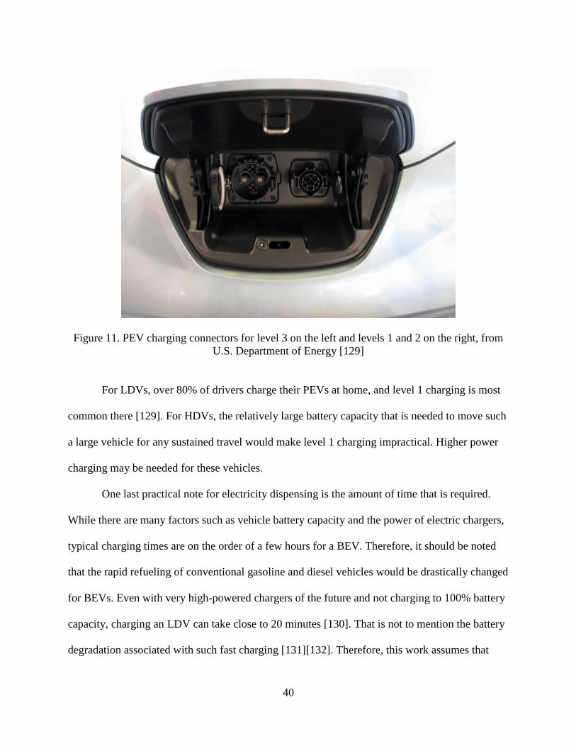
40

Figure 11. PEV charging connectors for level 3 on the left and levels 1 and 2 on the right, from

U.S. Department of Energy [129]

For LDVs, over 80% of drivers charge their PEVs at home, and level 1 charging is most

common there [129]. For HDVs, the relatively large battery capacity that is needed to move such

a large vehicle for any sustained travel would make level 1 charging impractical. Higher power

charging may be needed for these vehicles.

One last practical note for electricity dispensing is the amount of time that is required.

While there are many factors such as vehicle battery capacity and the power of electric chargers,

typical charging times are on the order of a few hours for a BEV. Therefore, it should be noted

that the rapid refueling of conventional gasoline and diesel vehicles would be drastically changed

for BEVs. Even with very high-powered chargers of the future and not charging to 100% battery

capacity, charging an LDV can take close to 20 minutes [130]. That is not to mention the battery

degradation associated with such fast charging [131][132]. Therefore, this work assumes that

41

more modest charging powers of level 1 and level 2 charging will be used to prevent damage to

the battery, in addition to economic considerations that will be discussed later.

2.1.4.2 Hydrogen Dispensing

Hydrogen dispensing stations, often called hydrogen refueling stations (HRSs), are new,

rare, and expensive. There are 40 stations open in California as of May 2019 [133]. There are

some stations on the east coast [134], but otherwise hydrogen dispensing stations are non-

existent in the rest of the U.S. Therefore, any significant future adoption of hydrogen vehicles

will require hydrogen dispensing station construction. Current small-scale hydrogen stations

costing on the order of $1 million each [135].

Note that the hydrogen station schematic is quite similar to that of the SNG station, as

seen in Figure 12. One major difference is that because pipeline distribution of hydrogen is not

modeled in this work, the “gas line” of the SNG station would be a tube trailer of liquid

hydrogen that is delivered by truck.

2.1.4.3 SNG Dispensing

SNG is distributed just like compressed natural gas (CNG). CNG stations, while mature

like gasoline and diesel stations, are not nearly as common. CNG is an option for HDVs and was

until recently an option for LDVs. There are 116 public CNG stations that can support fueling

for HDVs as of June 2019 [136]. However, neither the LDV nor HDV options have become as

prevalent as the gasoline and diesel options, and similarly neither have CNG dispensing stations

become as prevalent as gasoline and diesel dispensing stations. Therefore, any significant future

adoption of SNG vehicles will require SNG fueling station construction [137].

42

A schematic representation of a SNG station is shown in Figure 12, with the “gas line”

input being the natural gas pipeline that is used for distribution of SNG.

Figure 12. SNG dispensing station schematic, from U.S. Department of Energy [138]

2.1.4.4 Renewable Gasoline and Diesel Dispensing

Renewable gasoline and diesel are both drop-in fuels, and therefore can be sold at

existing gasoline and diesel stations. Gasoline for LDVs and diesel for HDVs are the primary

fuels today, and their fueling infrastructure is prevalent. In fact, many intersections have multiple

gasoline and diesel stations to choose for fueling. Therefore, no significant infrastructure would

need to be built for these fuels into the future.

2.1.5 Fuel Emissions

Emissions from fuel for this work are considered only from the feedstock, whether

electricity or biomass, and the overall pathway efficiency. However, efficiency of the various

steps, including distribution and dispensing is considered and therefore has an effect on the

emissions associated with the vehicle fuel.

43

Not included are leakage emissions from distribution, particularly applicable for gaseous

fuels such as hydrogen and SNG. GREET notes that 1.3% of US natural gas throughput is

emitted into the air as methane. This methane comes from both leakage from extraction,

processing, and distribution, as well as some combustion used for heat for any needed process.

GREET also notes that about 0.2% of natural gas is leaked in transmission from the natural gas

processing plant to electric generators that run on natural gas. Therefore, the leakage that can be

assumed for the distribution of SNG falls somewhere between the above two numbers. Overall,

this value is negligible and will not be considered a loss in this work. The same is assumed for

hydrogen, which has been shown to be about 1.5 to 3 times faster to escape from an

intentionally-manufactured leak [139]. Even at this slightly increased leakage, the rate is still

negligible. Similarly, distribution of renewable gasoline and diesel are assumed to be leak-free.

Electricity is not leaked, but distribution efficiency will be included.

2.2 Vehicle Powertrains

Vehicles will be separated into two categories for this work: light-duty vehicles (LDVs)

and heavy-duty vehicles (HDVs). LDVs include passenger vehicles that most of the public drives

for daily transportation needs. Included in this category are sedans, sport utility vehicles (SUVs),

minivans, small pick-up trucks, and other similar vehicles. HDVs are classified by their weight.

In fact, all such large vehicles are classified into a scheme from Class 1 through Class 8 based on

their gross vehicle weight rating (GVWR), which is the total weight of the loaded vehicle

including cargo. The present work focuses on only Class 8 HDVs, which are 33,001 pounds and

greater. These Class 8 HDVs are responsible for the most vehicle miles traveled (VMT) of any

vehicle category [140], as shown in Figure 13. Class 8 HDVs are also responsible for a large

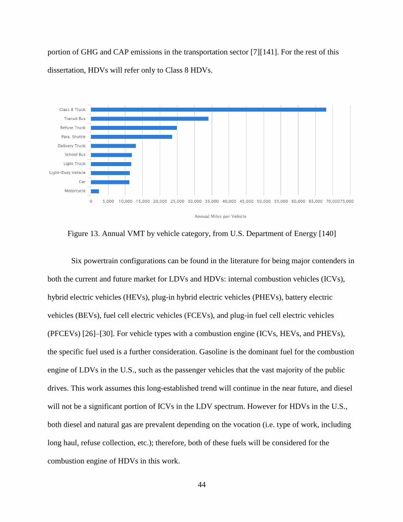
44

portion of GHG and CAP emissions in the transportation sector [7][141]. For the rest of this

dissertation, HDVs will refer only to Class 8 HDVs.

Figure 13. Annual VMT by vehicle category, from U.S. Department of Energy [140]

Six powertrain configurations can be found in the literature for being major contenders in

both the current and future market for LDVs and HDVs: internal combustion vehicles (ICVs),

hybrid electric vehicles (HEVs), plug-in hybrid electric vehicles (PHEVs), battery electric

vehicles (BEVs), fuel cell electric vehicles (FCEVs), and plug-in fuel cell electric vehicles

(PFCEVs) [26]–[30]. For vehicle types with a combustion engine (ICVs, HEVs, and PHEVs),

the specific fuel used is a further consideration. Gasoline is the dominant fuel for the combustion

engine of LDVs in the U.S., such as the passenger vehicles that the vast majority of the public

drives. This work assumes this long-established trend will continue in the near future, and diesel

will not be a significant portion of ICVs in the LDV spectrum. However for HDVs in the U.S.,

both diesel and natural gas are prevalent depending on the vocation (i.e. type of work, including

long haul, refuse collection, etc.); therefore, both of these fuels will be considered for the

combustion engine of HDVs in this work.

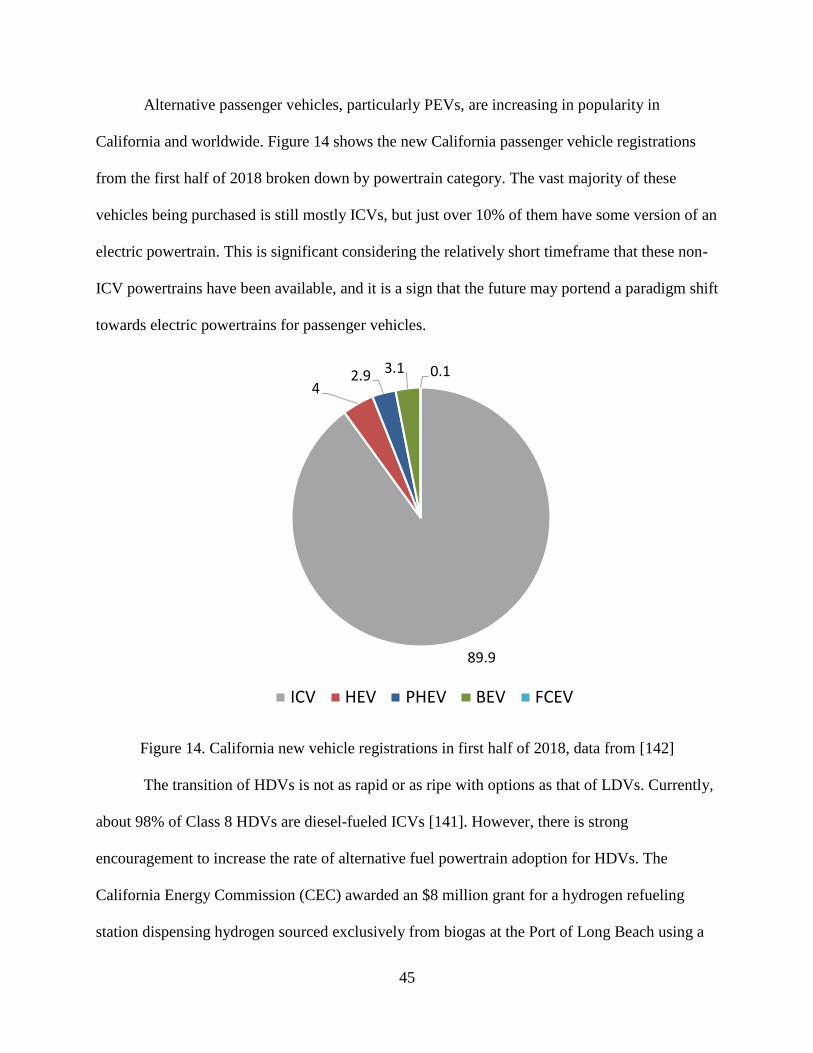
45

Alternative passenger vehicles, particularly PEVs, are increasing in popularity in

California and worldwide. Figure 14 shows the new California passenger vehicle registrations

from the first half of 2018 broken down by powertrain category. The vast majority of these

vehicles being purchased is still mostly ICVs, but just over 10% of them have some version of an

electric powertrain. This is significant considering the relatively short timeframe that these non-

ICV powertrains have been available, and it is a sign that the future may portend a paradigm shift

towards electric powertrains for passenger vehicles.

Figure 14. California new vehicle registrations in first half of 2018, data from [142]

The transition of HDVs is not as rapid or as ripe with options as that of LDVs. Currently,

about 98% of Class 8 HDVs are diesel-fueled ICVs [141]. However, there is strong

encouragement to increase the rate of alternative fuel powertrain adoption for HDVs. The

California Energy Commission (CEC) awarded an $8 million grant for a hydrogen refueling

station dispensing hydrogen sourced exclusively from biogas at the Port of Long Beach using a

89.9

42.9 3.1 0.1

ICV HEV PHEV BEV FCEV

46

technology known as tri-generation to produce electricity, heat, and hydrogen fuel [140][143].

Grants like this along with the laws, regulations, and goals from Table 1 show the focus on

transitioning HDVs to cleaner technology.

Important to note are different vocations for HDVs. While LDVs typically serve only to

transport drivers from one location to another, HDVs are specialized in a particular task or set of

tasks. These tasks vary from transporting goods from ports to distribution centers, hauling goods

long distances, collecting trash from communities and delivering it to landfills, and many others.

For this work, four vocations are selected based on total number of miles traveled in California

and the relative impact they have on air quality through CAP emissions. The four vocations

considered are as follows: (1) linehaul, which transport goods long distances, (2) drayage, which

transport goods from ports to distribution centers, (3) refuse, which collect waste from various

locations and transport it to processing centers or landfills, and (4) construction, which move

construction material or assist in construction of buildings and other built structures.

Vehicle emissions are composed of the emissions from the vehicles tailpipe and also

include other emissions such as tire and brake emissions. While tire and brake emissions do

depend on vehicle mass (which varies from one vehicle powertrain to another), this factor is not

considered in this work. Therefore, all vehicle powertrains are assumed to have the same tire and

brake emissions. Due to this assumption, there is no comparative advantage between powertrain

configurations in this modelling, so these tire and brake emissions are neglected in this work.

The BEV, FCEV, and PFCEV are all zero-emission vehicles (ZEVs), meaning there are

no tailpipe emissions from these vehicles. All other powertrain configurations have tailpipe

emissions that must be analyzed.

47

Regarding HDVs, there has been recent advancement in ICV engines which are referred

to as low-nitrogen oxides (low-NOx) engines. Both diesel and CNG engines have low-NOx

variations that are either available now (for CNG) or expected to be on the market in the next

few years (for diesel) [144]. These standards set limits of 0.02 grams of NOx emission for each

brake horsepower-hour of operation [145], [146]. It is assumed that any HDVs that are fueled by

either SNG or renewable diesel in this modelling effort will be low-NOx engines, once the

technology has become available. More information on the availability of low-NOx diesel

engines will be detailed in a later section of this dissertation.

2.2.1 ICV

ICVs have been the primary vehicle type in recent history, after a short stint of BEV

popularity when passenger vehicles were first introduced [147]. ICVs use a hydrocarbon fuel

(typically gasoline for LDVs and diesel for HDVs). This fuel is combusted in the engine which,

through mechanical linking of the powertrain, leads to the spinning of the vehicle’s wheels. The

combustion process leads to tailpipe GHG and CAP emissions from these vehicles.

For HDVs, SNG is also a fuel for ICVs (as well as any other powertrain with a

combustion engine such as HEVs and PHEVs). SNG is a gaseous fuel, so to store any reasonable

quantity of fuel on the vehicle, SNG must be stored either at pressure or a liquid after being

liquefied. Storing as a gas is more prevalent in vehicles and also more efficient as it does not

require the energy intensive and costly step of liquefying. Either option requires a robust tank

that is able to withstand significant pressure.

48

2.2.2 HEV

HEVs add a traction battery and electric motor to the ICV powertrain to gain efficiency

in moving the vehicle. The addition of the battery and electric motor offer two main benefits

over the ICV. First, the HEV can recharge its battery when braking by running the electric motor

in reverse, as a generator. This is known as regenerative braking and is done instead of or in

addition to the brakes of the vehicle, which has the additional benefit of extending brake pad life.

Regenerative braking reduces the amount of fuel needed because the battery helps accelerate and

drive the vehicle instead of using just fuel in the combustion engine. In addition to regenerative

braking, HEVs also allow the engine to run at more efficient operating conditions while the

battery works on the dynamic portions of the power demand.

HEVs trace back to the end of the 19th century, but their presence soon died out as ICVs

became the vehicle type of choice [148]. However, with the ZEV Action Plan of 1990,

automakers were to make increasing numbers of ZEVs for California sale staring in 1998 [18]. In

later revisions of the plan, cars with very low emissions known as partial ZEVs (PZEVs) were

eligible to help meet the goals [149]. The HEV was a method for automakers to work towards

complying with the ZEV Action Plan, though they were not clean enough to count as a PZEV.

2.2.3 PHEV

The evolution of the HEV is the PHEV. Quite similar to HEVs, PHEVs have two major

benefits stemming from the inclusion of a larger traction battery than the HEV: (1) a modest

battery electric range (BER) and (2) recharging of the traction battery from an external electricity

supply, which classifies the PHEV as a PEV. This allows for efficient and tailpipe emissions-free

49

driving for a limited range, but does not limit drivers to only go short distances as a combustion

engine works as a range extender.

Note the acronym BER instead of the conventional acronym all electric range (AER).

While the battery is the only source of electric power in the PHEV powertrain, this is not always

true. Therefore, the conventional acronym AER is not adequate to describe driving range

powered by the traction battery of a vehicle. The new acronym BER is used to distinguish

between the traction battery and the other power source, whether that other power source is

electric or not.

Due to the dramatic emissions reductions of PHEVs compared to HEVs (25-50% for

carbon dioxide [150]), PHEVs are classified as PZEVs and so comply with the ZEV Action Plan.

While PHEVs are attractive for the above reasons, they do use combustion engines and

therefore have tailpipe GHG and CAP emissions. For this reason, PHEVs may prove to be a

transitional vehicle into a future of vehicles that have no tailpipe emissions.

2.2.4 BEV

BEVs are powered by a traction battery, typically significantly larger than that of PHEVs.

This increased size is needed as the battery is the sole source of power to move the vehicle.

Refueling the BEV is done by connecting the vehicle to some electricity source. Typically, this

electricity source is the electric grid, but with the right equipment, it would be possible to

recharge the BEV (or any other PEV) from off-grid renewable electricity.

Before Henry Ford’s ICV revolution in the early 20th century, BEVs were the vehicle

powertrain of choice for some time [147]. Due to the focus on reducing emissions society-wide

50

as well as improving battery technology, BEVs are regaining popularity and sales are

dramatically increasing [151].

Because there is no combustion engine in a BEV, there are no tailpipe emissions. In fact,

there is no tailpipe at all. BEVs also have very high efficiency compared to most other vehicle

types. However, they typically cannot drive as far or refuel as fast as other vehicle types [152]. In

the case of LDVs, even if drivers are able to charge their BEVs at home (given they have access

to a charging outlet at home), the inconvenience of a long charge time can dissuade drivers from

purchasing BEVs.

Recent improvements in battery technology bring approximately 200 mile driving range

to BEVs in a more-affordable price range. Additionally, PEV chargers are increasing their

charging rates, allowing for shorter charging times [153]–[155].

While BEVs do not have tailpipe emissions, they can indirectly create emissions

depending on the source of the electricity charging them. If a BEV is charged using only

renewable sources, it is effectively emission-free (aside from other life-cycle emissions such as

manufacturing that is beyond the scope of this work). However, if the BEV is charged from the

California electric grid, it has emissions associated with the natural gas power plants that, along

with the emissions-free renewables, are part of the electric grid. There is a trend of increasing

emission-free electricity, particularly in California, so the emissions of BEVs (and all PEVs) are

decreasing accordingly [156].

For HDVs, long charging time and short driving range can severely limit the types of

work these vehicles are able to do. Therefore, careful consideration must be given for BEV

adoption in the HDV sector. As of 2015, only drayage and refuse trucks had been demonstrated

to operate with a BEV powertrain [157]. While improving battery and charging technology may

51

increase the aptitude of heavy-duty BEVs, current thinking is that BEVs will have a limited role

in the heavy-duty sector, particularly with regard to range. Further consideration of this issue will

be discussed in a later section.

Note that catenary HDVs, which use external electrified lines to charge the battery of a

vehicle (whether BEV or any PEV), are not considered in this work due to the necessity of

spatial resolution. Catenary technology is best suited for particular sections of a highway that

may cause trouble for a HDV relying on batteries, for example, an extended incline, and that

spatial resolution is not within the scope of this work [157]. This does not mean, however, that

catenary HDVs will not play a role in helping to electrify some HDV areas. This work assumes

that application of catenary HDVs will be done on a case-by-case basis in a limited number of

locations.

2.2.5 FCEV

FCEVs are powered by a fuel cell. A fuel cell is an electrochemical device, similar to a

battery. The main difference is a battery stores its fuel and oxidant within the housing of the

battery itself. A fuel cell stores these two outside, with the fuel in a tank and oxidant often being

ambient air. This key difference allows for the power and energy to be scaled independently for

fuel cells, unlike batteries. FCEVs use proton exchange membrane fuel cells (PEMFCs) as they

are relatively low temperature (below 100 oC) and handle dynamic operation better than other

fuel cell varieties. PEMFCs operate on hydrogen fuel. Because hydrogen is a gas with relatively

low volumetric energy density, it must be compressed to very high pressures (typically 70 MPa

for LDVs, and roughly half that for HDVs) for vehicular use. A schematic diagram of a PEMFC

is shown in Figure 15. One important note is that, despite not being in the name, FCEVs are

52

typically hybrids with a traction battery installed to allow for regenerative braking and efficient

fuel cell operation. FCEVs in this work are assumed to be hybrids.

Figure 15. Schematic of PEM Fuel Cell, from U.S. Department of Energy [158]

FCEVs are new to the commercial market, with an introduction in the mid-2010s. Their

overall emissions are dependent on the method of fuel production (of which there are many

options, as has been detailed). Nearly all of the current production of hydrogen in the U.S. is

from natural gas by SMR [53]. This will likely change in future as, already, California requires at

least one third of the hydrogen sold at fueling stations has to have a renewable feedstock if that

station receives State funds [20]. This requirement will necessarily increase the use of biomass

and renewable electricity in hydrogen production.

In practice, FCEVs share similarities to both BEVs and ICVs. Like BEVs, FCEVs have

no tailpipe emissions, other than the small amount of water produced by the fuel cell, and

53

relatively high efficiency, though not as high as that of BEVs [14]. Like ICVs, refueling FCEVs

is fast, nearly as fast as refueling a gasoline or diesel vehicle. Additionally, driving range is also

comparable to ICVs due to the independent sizing of power and energy, so an adequately-sized

hydrogen tank can be incorporated. The former qualities make an environmentally-friendly

vehicle. The latter qualities make a vehicle convenient for drivers.

While the above is true in theory, the current lack of hydrogen fueling infrastructure

means fueling is not yet very convenient for drivers unless they happen to live and travel near

one of the 40 California stations open as of June 2019 [133]. This becomes less of an issue with

time as the fueling infrastructure develops. However, the FCEV market is affected by the low

number of hydrogen fueling stations, but costly stations are hard to justify without higher FCEV

adoption. This is proving to be a challenge for FCEVs that could be overcome by optimism in

the market. For example, the California Energy Commission has recently awarded an $8 million

grant for a hydrogen station at the Port of Long Beach which will use 100% biogas [159].

2.2.6 PFCEV

The PFCEV shares similarities with the FCEV and PHEV. From a systems level, the

PFCEV operates the same as a PHEV; however, instead of a combustion engine, the PFCEV has

a fuel cell and it is fueled by hydrogen. A schematic of a PFCEV powertrain can be seen in

Figure 16. Note that all of the powertrain components are electric. This increases the efficiency

compared to the PHEV as it removes the efficiency loss of converting from mechanical energy

of a combustion engine to electrical energy through an electric generator.

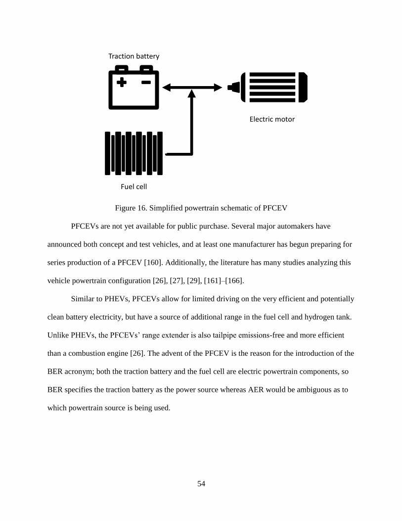
54

Figure 16. Simplified powertrain schematic of PFCEV

PFCEVs are not yet available for public purchase. Several major automakers have

announced both concept and test vehicles, and at least one manufacturer has begun preparing for

series production of a PFCEV [160]. Additionally, the literature has many studies analyzing this

vehicle powertrain configuration [26], [27], [29], [161]–[166].

Similar to PHEVs, PFCEVs allow for limited driving on the very efficient and potentially

clean battery electricity, but have a source of additional range in the fuel cell and hydrogen tank.

Unlike PHEVs, the PFCEVs’ range extender is also tailpipe emissions-free and more efficient

than a combustion engine [26]. The advent of the PFCEV is the reason for the introduction of the

BER acronym; both the traction battery and the fuel cell are electric powertrain components, so

BER specifies the traction battery as the power source whereas AER would be ambiguous as to

which powertrain source is being used.

Traction battery

Electric motor

Fuel cell

55

2.2.7 Vehicle Components

Having described each of the vehicle powertrains considered in this work, it is helpful to

now summarize the various components of these vehicles that will be combined to determine an

overall vehicle cost in this work. These components are listed in Table 5.

Table 5. Vehicle components considered

COMPONENT COMPONENT DESCRIPTION

Glider, LDV The LDV glider includes all of the vehicle components that are not part of the powertrain.

This includes parts such as the chassis, wheels, windows, etc.

Glider, HDV The HDV glider includes all of the vehicle components that are not part of the powertrain.

This includes parts such as the chassis, wheels, windows, etc.

IC engine,

gasoline

For LDVs, the gasoline IC engine is the sole power plant of ICVs, as well as a co-power

plant (along with a battery) of HEVs and PHEVs

IC engine, diesel For HDVs, the diesel IC engine is one option for the power plant of ICVs, as well as a co-

power plant (along with a battery) of HEVs and PHEVs

IC engine, SNG For HDVs, the SNG IC engine is one option for the power plant of ICVs, as well as a co-

power plant (along with a battery) of HEVs and PHEVs

Fuel cell The fuel cell is the sole power plant of FCEVs and co-power plant of PFCEVs

Traction battery The traction battery is the sole power plant of BEVs, and co-power plant of HEVs, PHEVs,

FCEVs, and PFCEVs

Electric motor /

generator

The electric motor is used in all electric powertrains (HEV, PHEV, BEV, FCEV, and

PFCEV) to convert electrical energy to motion of the wheels, and it can be run in reverse as

a generator to convert wheel motion into electric energy

Liquid fuel tank The liquid fuel tank holds gasoline or diesel for ICVs fueled by those liquid fuels

SNG tank The SNG tank is a stronger, more robust tank that holds pressurized SNG (typically around

25 MPa [167]) for HDVs fueled by SNG, which is typically stored as a gaseous fuel

Hydrogen tank

The hydrogen tank is an even stronger and more robust tank that holds pressurized hydrogen

(typically at 70MPa) for vehicles fueled by hydrogen, which is typically stored as a gaseous

fuel

Hybrid adder,

LDV

The LDV hybrid adder accounts for various equipment beyond the traction battery and

electric motor (i.e. controls, wiring, etc.) needed to convert a LDV powertrain into its

equivalent hybrid one

Hybrid adder,

HDV

The HDV hybrid adder accounts for various equipment beyond the traction battery and

electric motor (i.e. controls, wiring, etc.) needed to convert a HDV powertrain into its

equivalent hybrid one

Plug-in hybrid

adder, LDV

The LDV plug-in hybrid adder accounts for various equipment beyond the traction battery

and electric motor (i.e. controls, wiring, etc.) needed to convert a LDV powertrain into its

equivalent plug-in hybrid one

Plug-in hybrid

adder, HDV

The HDV plug-in hybrid adder accounts for various equipment beyond the traction battery

and electric motor (i.e. controls, wiring, etc.) needed to convert a HDV powertrain into its

equivalent plug-in hybrid one

56

2.3 Optimization and Linear Programming

So far, many vehicle fuel production pathways have been introduced. Furthermore,

several vehicle types that can use those fuels have been introduced. Together, there is a wide

range of potential options that can be pursued for the transportation sector. In a problem as

complex as this, it is important to have a systematic and objective approach.

Consider the Sankey diagram in Figure 17. Currently, the vast majority of transportation

is fueled by petroleum. Additionally, one can see the amount of energy needed for transportation

near the bottom-right corner (5.91 quadrillion British thermal units) as well as the various

resources that can be utilized to meet that demand on the left side. It is clear that there is no one

carbon-free source that can meet the transportation needs, whether that is biomass or some

renewable source of electricity. Therefore, some methodology is needed to determine what

combination of fuel sources and pathways should be pursued to meet our societal goals at the

lowest cost. The proposed methodology of doing so is optimization.

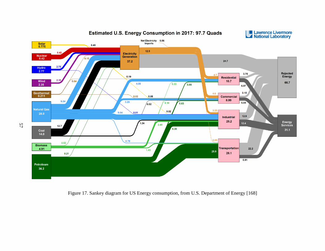
57

Figure 17. Sankey diagram for US Energy consumption, from U.S. Department of Energy [168]

63

Optimization is a mathematical methodology which selects the “optimal” option from a

given set of possibilities. Here, “optimal” is defined using what is known in the optimization

discipline as the cost (or objective) function. Each possible solution has an associated cost which

is defined by this cost function. Note that the word “cost” here can be a misnomer in that the cost

of an objective function does not necessarily have to be the cost in colloquial terms (though in

the optimization problem of this dissertation it is). Optimization problems are typically set up to

select from the possible solutions the one with the minimum cost. However, some optimization

does attempt to maximize the cost function, which is often done when the cost function is

actually reflecting a profit. Converting from a maximizing optimization problem to a minimizing

optimization problem can be done by simply multiplying the cost function by negative one.

In addition to the cost function, optimization often includes constraints. These are

mathematical representations that prevent certain solutions from being chosen for any desired

reason, such as physical impossibility or respecting an existing regulation.

The cost function and constraints are perhaps best explained by a simple example, as follows.

Imagine you are in charge of managing how electricity is generated, with multiple electricity

generators at your control. Each generator has its own cost associated with producing a given

amount of electricity. You must produce the exact amount of electricity that is demanded by

those using the electricity in the area (this is due to the fact that there is no significant storage in

the electric grid). In this example, the cost function that must be minimized is the total cost of

using each of the generators to produce electricity. The constraint is that the total electricity

produced by all of the generators is equal to the electricity demand. This minimization problem

can be written mathematically with the minimization of the cost function which is the total cost

of producing electricity shown in Equation 4, and the constraints which require electricity

production must be equal to demand shown in

Equation 5. In Equation 4 and Equation 5, n is the number of electricity generators

available, genCosti is the cost of producing electricity from the ith generator, xi is the amount of

electricity chosen to be generated by the ith generator, and electricityDemand is the amount of

electricity that must be generated to meet demand.

63

Equation 4. Example minimization cost function

min∑𝑔𝑒𝑛𝐶𝑜𝑠𝑡𝑖 ∗ 𝑥𝑖

𝑛

𝑖=1

Equation 5. Example minimization constraints

∑𝑥𝑖 = 𝑒𝑙𝑒𝑐𝑡𝑟𝑖𝑐𝑖𝑡𝑦𝐷𝑒𝑚𝑎𝑛𝑑

𝑛

𝑖=1

Note that optimization problems can have a single cost function to minimize (or

maximize) or multiple cost functions to minimize (or maximize). In the case of multiple cost

functions, a weighting must be established to determine priority of costs in finding the optimal

solution. Different costs allow for optimizing with respect to different qualities, such as money

spent, emissions output, driving range, or societal happiness. Note that these costs may be

somewhat qualitative, but as long as a value can be artificially applied to them, they can be

represented as a cost function. This dissertation uses a single cost function, which is money

spent. Emissions, another major parameter included in this work, are included as constraints.

Linear programming (LP) is a subset of optimization in which the cost function(s) and

each of the constraints is linear. This means that of every term in the cost function(s) and

constraints, there is at least one term that is of mathematical order one, and there are no terms of

higher order. Linear programming is less computationally intensive than non-linear

programming, leading to solutions that converge much faster and consistently. In general, it is

advisable to attempt to linearize a non-linear problem using approximations to make solving the

programming problems faster and better-behaved (better convergence).

A common subset of LP is mixed integer LP (MILP). This subset allows for some

variables to be constrained as integers, which may be appropriate for some problems. Consider

63

for example, a problem with number of people as a variable. There can be no fraction of people,

so a MILP approach is appropriate.

However, this care in keeping certain variables as integers may be relaxed based on the

scale of the problem and the desired detail of results. One could imagine that for some work, the

difference in knowing there are, hypothetically, 14,500,000 vehicles on the road in California

versus 14,500,001 vehicles is so small that the practical difference is often negligible.

Furthermore, an estimate of 14,500,000.5 vehicles, while physically nonsensical, could very

appropriately be rounded up to 14,500,001 vehicles without issue in most scenarios. Therefore,

even some problems which may at first seem appropriate for a MILP approach may be satisfied

by a relaxation to a LP without the integer variables constraint. This would improve solving time

without practical detriment to the results.

2.4 Literature Review

This section reviews the literature relevant to the scope of this work. There are two

sections of literature review: first, analyzing and comparing either a single or multiple fuel

pathways, and second, a supply chain optimization that considers multiple fuel pathways and

optimizes them according to some cost function.

2.4.1 Literature Review of Individual or Multiple Fuel Pathways Compared

Before attempting to optimize fuel production and vehicle powertrain pathways, it is wise

to assess the individual characteristics of each pathway. Much of the literature is split between

work on electrolytic fuels and work on biomass-sourced fuels. There is not much work that

compares fuels coming from the two different feedstocks.

63

Bertuccioli et al. is a techno-economic assessment of hydrogen production pathways,

with AEC and PEMEC electrolyzer technology improvements. Major contributions of this work

are the efficiency and cost of both AEC and PEMEC technology with projections to 2030, as

well as distribution and dispensing considerations [169]. Not included in this work are data for

SOECs or analysis of vehicles. Also, projections were only made to 2030, not to 2050 as in the

present work.

Schmidt et al. is another notable techno-economic work for electrolytic hydrogen

pathways, including a ten-expert survey of five academics and five industry representatives.

Included electrolyzer technologies are AEC, PEMEC, and SOEC [170]. Only fuel production is

considered, and there are no emissions considerations. Like Bertuccioli et al., projections were

also only made out to 2030.

Ramsden et al. have evaluated the current state of 10 P2G pathways and determined their

associated levelized cost of hydrogen and greenhouse gas emissions. Data used for this analysis

are sourced primarily from the H2A Production Model, the Hydrogen Delivery Scenario

Analysis Model, GREET, and the Cost-per-Mile Tool. The updated version of the report

includes, in addition to up-to-date data, additional P2G pathways that add up to the 10 mentioned

as well as more analysis with FCEVs. The pathway with distributed natural gas reforming led to

the lowest levelized cost of hydrogen, and the pathway with distributed ethanol reforming led to

the highest levelized cost of hydrogen [171]. This work is notable for its comprehensive analysis

of all major portions of the fuel pathway, including fuel production, distribution, dispensing, and

use in vehicles. This comprehensive framework serves as an example of work to be carried out

both into the future as well as for other fuels, neither of which are included in this work.

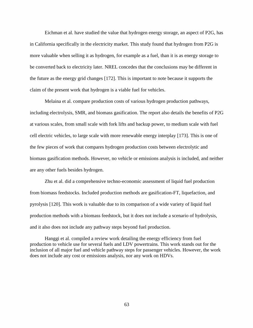
63

Eichman et al. have studied the value that hydrogen energy storage, an aspect of P2G, has

in California specifically in the electricity market. This study found that hydrogen from P2G is

more valuable when selling it as hydrogen, for example as a fuel, than it is as energy storage to

be converted back to electricity later. NREL concedes that the conclusions may be different in

the future as the energy grid changes [172]. This is important to note because it supports the

claim of the present work that hydrogen is a viable fuel for vehicles.

Melaina et al. compare production costs of various hydrogen production pathways,

including electrolysis, SMR, and biomass gasification. The report also details the benefits of P2G

at various scales, from small scale with fork lifts and backup power, to medium scale with fuel

cell electric vehicles, to large scale with more renewable energy interplay [173]. This is one of

the few pieces of work that compares hydrogen production costs between electrolytic and

biomass gasification methods. However, no vehicle or emissions analysis is included, and neither

are any other fuels besides hydrogen.

Zhu et al. did a comprehensive techno-economic assessment of liquid fuel production

from biomass feedstocks. Included production methods are gasification-FT, liquefaction, and

pyrolysis [120]. This work is valuable due to its comparison of a wide variety of liquid fuel

production methods with a biomass feedstock, but it does not include a scenario of hydrolysis,

and it also does not include any pathway steps beyond fuel production.

Hanggi et al. compiled a review work detailing the energy efficiency from fuel

production to vehicle use for several fuels and LDV powertrains. This work stands out for the

inclusion of all major fuel and vehicle pathway steps for passenger vehicles. However, the work

does not include any cost or emissions analysis, nor any work on HDVs.

63

Table 6 summarizes the key literature in this area, including that mentioned above as well

as other studies in this field.

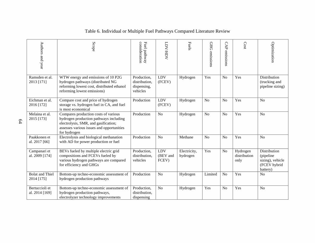
64

Table 6. Individual or Multiple Fuel Pathways Compared Literature Review

Au

tho

rs and

year

Sco

pe

Fu

el path

way

con

sideratio

n

LD

V/H

DV

Fu

els

GH

G em

ission

s

CA

P em

ission

s

Co

st

Op

timizatio

n

Ramsden et al.

2013 [171]

WTW energy and emissions of 10 P2G

hydrogen pathways (distributed NG

reforming lowest cost, distributed ethanol

reforming lowest emissions)

Production,

distribution,

dispensing,

vehicles

LDV

(FCEV)

Hydrogen Yes No Yes Distribution

(trucking and

pipeline sizing)

Eichman et al.

2016 [172]

Compare cost and price of hydrogen

storage vs. hydrogen fuel in CA, and fuel

is most economical

Production LDV

(FCEV)

Hydrogen No No Yes No

Melaina et al.

2015 [173]

Compares production costs of various

hydrogen production pathways including

electrolysis, SMR, and gasification;

assesses various issues and opportunities

for hydrogen

Production No Hydrogen No No Yes No

Paakkonen et

al. 2017 [66]

Electrolysis and biological methanation

with AD for power production or fuel

Production No Methane No No Yes No

Campanari et

al. 2009 [174]

BEVs fueled by multiple electric grid

compositions and FCEVs fueled by

various hydrogen pathways are compared

for efficiency and GHGs

Production,

distribution,

vehicles

LDV

(BEV and

FCEV)

Electricity,

hydrogen

Yes No Hydrogen

distribution

only

Distribution

(pipeline

sizing), vehicle

(FCEV hybrid

battery)

Bolat and Thiel

2014 [175]

Bottom-up techno-economic assessment of

hydrogen production pathways

Production No Hydrogen Limited No Yes No

Bertuccioli et

al. 2014 [169]


hydrogen production pathways,

electrolyzer technology improvements

Production,

distribution,

dispensing

No Hydrogen Yes No Yes No

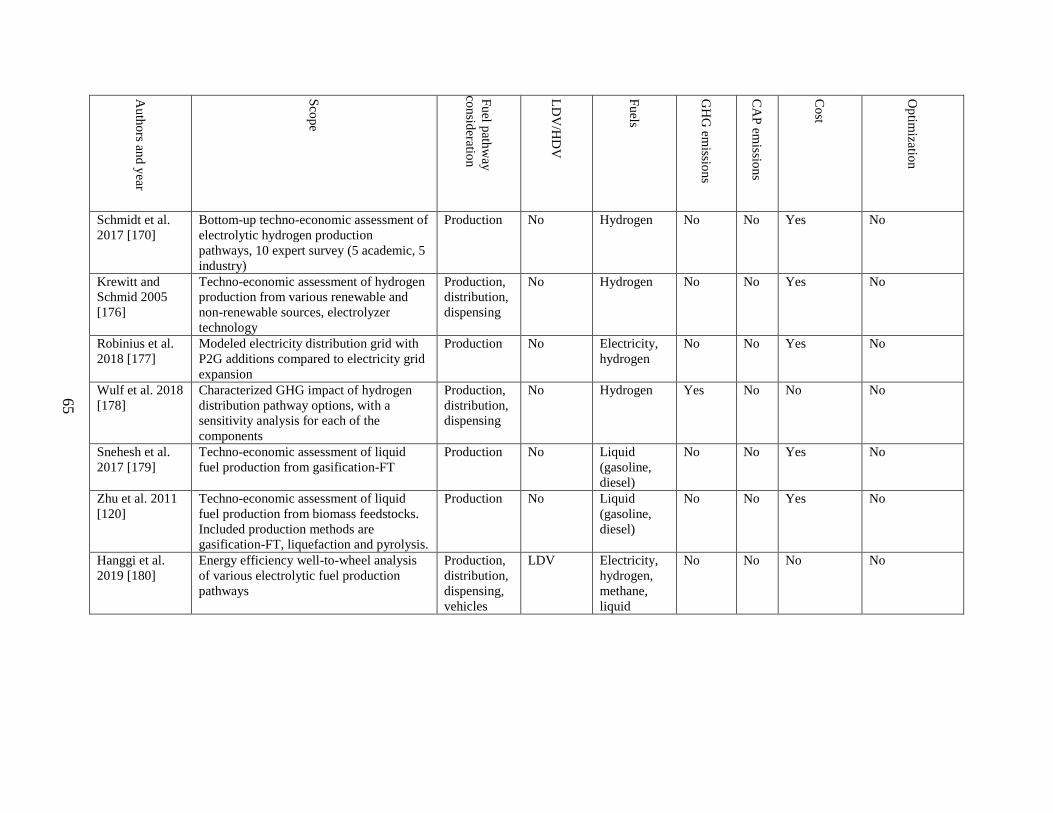
65

Au

tho

rs and y

ear

Sco

pe

Fu

el path

way

con

sideratio

n

LD

V/H

DV

Fu

els

GH

G em

ission

s

CA

P em

ission

s

Co

st

Op

timizatio

n

Schmidt et al.

2017 [170]


electrolytic hydrogen production

pathways, 10 expert survey (5 academic, 5

industry)

Production No Hydrogen No No Yes No

Krewitt and

Schmid 2005

[176]

Techno-economic assessment of hydrogen

production from various renewable and

non-renewable sources, electrolyzer

technology

Production,

distribution,

dispensing

No Hydrogen No No Yes No

Robinius et al.

2018 [177]

Modeled electricity distribution grid with

P2G additions compared to electricity grid

expansion

Production No Electricity,

hydrogen

No No Yes No

Wulf et al. 2018

[178]

Characterized GHG impact of hydrogen

distribution pathway options, with a

sensitivity analysis for each of the

components

Production,

distribution,

dispensing

No Hydrogen Yes No No No

Snehesh et al.

2017 [179]

Techno-economic assessment of liquid

fuel production from gasification-FT

Production No Liquid

(gasoline,

diesel)

No No Yes No

Zhu et al. 2011

[120]

Techno-economic assessment of liquid

fuel production from biomass feedstocks.

Included production methods are

gasification-FT, liquefaction and pyrolysis.

Production No Liquid

(gasoline,

diesel)

No No Yes No

Hanggi et al.

2019 [180]

Energy efficiency well-to-wheel analysis

of various electrolytic fuel production

pathways

Production,

distribution,

dispensing,

vehicles

LDV Electricity,

hydrogen,

methane,

liquid

No No No No

68

2.4.2 Literature Review of Supply Chain Optimization

Significant work has been done in the area of reducing emissions from transportation.

Focusing on the areas closely related to optimization in fuel pathways and powertrains, the work

can be narrowed down, and some of the standout work in this field are summarized below.

A study from d’Amore and Bezzo looked at minimizing the cost of carbon dioxide

capture, transport, and sequestration in Europe [181]. This work can be thought of as part of a

fuel production pathway, as carbon dioxide is needed to make SNG in the electrolytic pathways.

Here, an optimization with spatial consideration determines the lowest cost method of capturing

carbon dioxide from industrial and combustion processes and then transporting that carbon

dioxide to geologic locations to sequester it, or store it indefinitely, in Europe. While the

application of the optimization problem does not align too closely with the work of this

dissertation at it only considers carbon dioxide, the methodology shares similarities with the

present work but with an increased spatial focus.

Work by Angeles et al. looked at optimizing the production, transportation, and use of

ammonia as fuel in both ICVs and FCEVs [182]. This study includes both fuel production and

fuel use in a powertrain, but it is limited in scope to only one fuel and two powertrains.

Moreover, the use of ammonia as a fuel in vehicles is unlikely considering offerings from vehicle

manufacturers and general literature consensus. Therefore, the present work does not consider

ammonia as a future vehicle fuel. However, the work by Angeles et al. is still relevant due to the

methodology detailed within the work.

A study by Ribau et al. details optimization of efficiency, cost, and life cycle carbon

dioxide emissions for FCEV and PFCEV buses, particularly focusing on powertrain. This study

68

uses single- and multi-objective genetic algorithms with ADVISOR, a powertrain modeling tool

[162]. This study is noteworthy for including PFCEVs in addition to FCEVs and BEVs in the

robust optimization methodology, but it does not include other HDV fuels such as SNG or

renewable diesel.

Samsatli and Samsatli optimize considering cost, profit, and emissions various fuel

production pathways for electricity, hydrogen, SNG, and syngas in Great Britain. All pathway

sections, including feedstock, fuel production, distribution, dispensing, and vehicles are included

in the analysis, as well as projections out to 2050. However, vehicle work is minor, only

considering light-duty FCEVs. This work’s focus is on energy and heating demands, so

transportation analysis is a secondary consideration [183]. Drawbacks to this work, in addition to

the aforementioned minor vehicle analysis, include no liquid fuels consideration and no CAP

emissions analysis.

68

Table 7 summarizes the key literature in this area, including that mentioned above as well

as other studies in this field.

69

Table 7. Supply Chain Optimization Literature Review

Au

tho

rs and

year

Sco

pe

Fu

el path

way

con

sideratio

n

LD

V/H

DV

Fu

els

GH

G em

ission

s

CA

P em

ission

s

Co

st

Op

timizatio

n

d’Amore and

Bezzo 2017

[181]

Techno-economic work to minimize

the cost of carbon dioxide capture,

transport, and sequestration in Europe

Production,

distribution

No (Carbon

dioxide)

Yes No Yes Yes,

MILP

Angeles et al.

2017 [182]

Well-to-wheel analysis of fossil- and

bio-NH3 as a fuel for ICEVs or

FCEVs, minimizing carbon and

nitrogen emissions

Production,

distribution,

vehicles

Unspecified Ammonia Yes Yes No Yes, P-

graph

Ribau et al. 2014

[162]

Single- and multi-objective

optimization of FCEV and PFCEV

with comparison to diesel ICV,

including cost, efficiency, and lifetime

GHG emissions

Vehicles HDV (ICV,

FCEV, and

PFCEV)

Hydrogen,

electricity

Yes No Yes Yes,

genetic

Parker,

Tittmann, et al.

2010 [184]

Resource analysis and biorefinery

siting to optimize biomass use for

transportation fuel given price

Production,

distribution

No Liquid

biofuels

No No Yes Yes,

MILP

Parker, Fan, et

al. 2010 [49]

Analysis of economic potential and

infrastructure for H2 from biomass

Production,

distribution

No Hydrogen No No Yes Yes,

MINLP

Parker et al.

2017 [185]

Techno-economic model with

renewable CH4 supply curves, up to

2025

Production,

distribution

No Renewable

CH4

No No Yes Yes,

spatial

Zandi Atashbar

et al. 2018 [186]

Review paper of models and methods

to optimize biomass supply chains

Production,

distribution

No Biofuels Yes Yes Yes Yes,

mostly

MILP

Samsatli and

Samsatli 2018

[183]

Multi-objective MILP model with

evolution of electricity, H2, natural

gas, and syngas networks to 2050;

considers technological constraints

Production,

distribution,

dispensing,

vehicles

LDV

(FCEV)

Electricity,

H2, natural

gas, syngas

Yes No Yes Yes,

MILP

70

2.4.3 Background Summary

After introducing the vast number of options for alternative fuel production and

powertrain options for both LDVs and HDVs, it is apparent that a comprehensive, objective

methodology is needed to account for techno-economic data as well as fuel infrastructure and

vehicle use characteristics. The fuel production pathways and vehicle powertrain options detailed

in this chapter will serve as the map from which such a methodology will follow, adding to it the

necessary data and projections needed to comply with environmental legislation.

The key finding from the preceding literature review is that no work has analyzed and

optimized options for the breadth of fuels and vehicle powertrains to the extent of pathway

proposed in this work. In particular, the fuels to be included are electricity, hydrogen, SNG,

renewable gasoline, and renewable diesel; the vehicle powertrains to be included are ICV, HEV,

PHEV, BEV, FCEV, and PFCEV; and the pathway components to be included are fuel

production, distribution, dispensing, and use in vehicles.

A second finding is that LP appears to be an appropriate optimization tool for this work.

If the cost function and constraints allow for its use, LP will be the chosen optimization tool for

this work. For any cost or constraint that is not linear, care will be taken to effectively simplify

these non-linear components to linear ones.

This dissertation fills the gap in knowledge by establishing the viable fuel pathways and

powertrain configurations noted above for LDVs and HDVs. The fuel pathways and powertrain

configurations techno-economic data are projected out to 2050 and options are optimized using

LP to minimize the cost of complying with environmental constraints from the transportation

sector.

71

3. APPROACH


configurations for LDVs and HDVs that meet environmental constraints at the lowest cost. This

work develops a methodology to characterize and project various fuel pathways and powertrain

configurations techno-economic data and then determine a fleet to meet transportation needs into

2050. The results of this work will inform the transportation industry and policy makers how

society might effectively transform the transportation sector in a future of stricter environmental

regulations.

3.1 Tasks

To meet this dissertation goal, the following tasks will be completed.

Task 1. Establish the fuel pathways for LDVs and HDVs.

A literature review of the transportation sector will yield a list what fuels are being

considered for LDVs and HDVs as the State works toward cleaner vehicles across all vehicle

types and applications. Fuels come in the form of gaseous and liquid fuels, as well as electricity

in the case of PEVs.

Once the range of fuels has been selected, each one will be studied to determine its

pathway, that is, the steps that are followed from raw feedstock to finished fuel at the appropriate

dispensing station. Once each of the fuel pathways has been decomposed into its corresponding

individual steps, these steps can be further analyzed in the later Tasks for the techno-economic

analysis of this dissertation.

72

Task 2. Establish the powertrain configurations for LDVs and HDVs.

A literature review will expose the alternative fuel powertrains that should be included in

this study. The powertrains may vary based on classification, so each one will be considered

individually. Once the powertrains have been selected, each one will be studied to determine the

main components to consider, as a simplification of the vehicle as a whole without looking into

the various powertrain components may yield unrealistic results, particularly with respect to the

vehicle costs.

Note that the results of both Tasks 1 2 have been detailed in the Background of this

dissertation.

Task 3. Develop efficiency, cost, and emissions data out to 2050 for the fuel pathways

established in Task 1 and the vehicle powertrain configurations established in Task 2.

This Task is a comprehensive literature review to collect data of efficiency, cost, and

emissions of the various fuel pathways and powertrains. Additionally, this Task requires the

development of a methodology to project those data throughout the time horizon of analysis, up

to 2050. These projections will be the inputs to the optimization tool developed and run in later

Tasks.

Task 4. Establish the constraints of the optimization problem using California legislation and

executive order for emissions, realistic growth scenarios for travel and technology, and feedstock

availability.

Four classes of constraints are present in this optimization problem: emissions

regulations, VMT, realistic technology deployment, and feedstock availability. California

73

legislation will be consulted to determine the emissions regulations up to 2050; from these pieces

of legislation, constraints will be created for the WTW emissions from vehicles. VMT in

California are documented annually, and these will be extrapolated up to 2050 to create

constraints that must be met. Realistic technology deployment rates will constrain the problem

such that technologies cannot be deployed instantly or at rates that may not be feasible for a

number of practical reasons. Lastly, feedstock availability constraints must be considered as

there is only a limited amount of biomass and electricity that could be used to make vehicle

fuels.

Task 5. Determine optimization tool to use given the results of Tasks 3 and 4, and establish the

formal optimization problem.

Many optimization algorithms and software exist. This Task will focus on studying the

various algorithms and software, with the goal of determining which combination will be best

suited to this study. The method and software must take in the data developed in Task 3 and the

constraints developed in Task 4. The formal optimization problem is then established in this

Task, including the cost function and the constraints.

Task 6. Solve the optimization problem established in Task 5 to determine the emissions and

cost impacts of the optimum cases. Compare these results to the Reference Case.

Solving the optimization problem established in Task 5 will determine the mix of fuel

pathways and vehicle powertrain configurations that minimizes total cost of implementation

while still meeting California emissions legislation. Task 6 then develops a Reference Case of

conventional fuels (mainly gasoline and diesel) and conventional vehicle powertrains

74

(combustion engines) which is representative of the vehicle fleet today. The costs and emissions

associated with these fuels and vehicles will be calculated and serve as a Reference Case with

which to compare the alternatives studied in this work. Then, the optimization results will be

compared to the Reference Case to see the changes in emissions and the associated costs from

two alternative cases, a Non-ZEV Constrained Case and a ZEV-Constrained Case.

Task 7. Systematically assess the results to establish viable fuel pathways and powertrain

configurations for LDVs and HDVs that meet the constraints of this problem.

Task 7 uses the results of Task 6 to achieve the goal of this dissertation and provide

pathways for potential transportation sector evolution in the context of California’s legislation

and realistic constraints of adoption.

75

4. VEHICLE FUEL PATHWAYS

This chapter details the vehicle fuel production, distribution, and dispensing techno-

economic projections that are carried out to be inputs to the optimization problem.

Because the timescale of the present work is long (30 years from 2020 to 2050), inflation

must be considered. This work assumes a 2% rate of inflation, which is in line with recent

historic data from the U.S. [187].

Also needed due to the long timescale and the high capital costs of creating large fuel

production plants, the idea of a capital recovery factor (CRF) is introduced. A CRF is a method

of capturing various economic data such as interest rates, depreciation, lifetime of equipment,

and others to convert a single bulk capital cost into recurring payments. The present work

assumes a CRF of 0.12 for all equipment to calculate yearly payments from a single capital cost.

The precedent for this value is work from the U.S. Department of Energy using such a CRF for

its coal power plants for low-risk scenarios [188]. Inherent in using this CRF is the assumption

that the proceeding fuel production plants will be low-risk. This would mean that large entities

such as utilities would be the ones creating these plants, a valid assumption for a high-capital

plant. Also assumed is a lifetime of 30 years, which is the time of interest for this work.

Therefore, when a fuel production plant is built, it will be used until the end of the model run.

4.1 Fuel Feedstocks

Here, the cost of both electricity and biomass feedstocks is detailed. Emissions results are

presented at the end of this chapter, at which point both the feedstock emissions as well as the

total fuel pathway emissions up to the vehicle will be detailed.

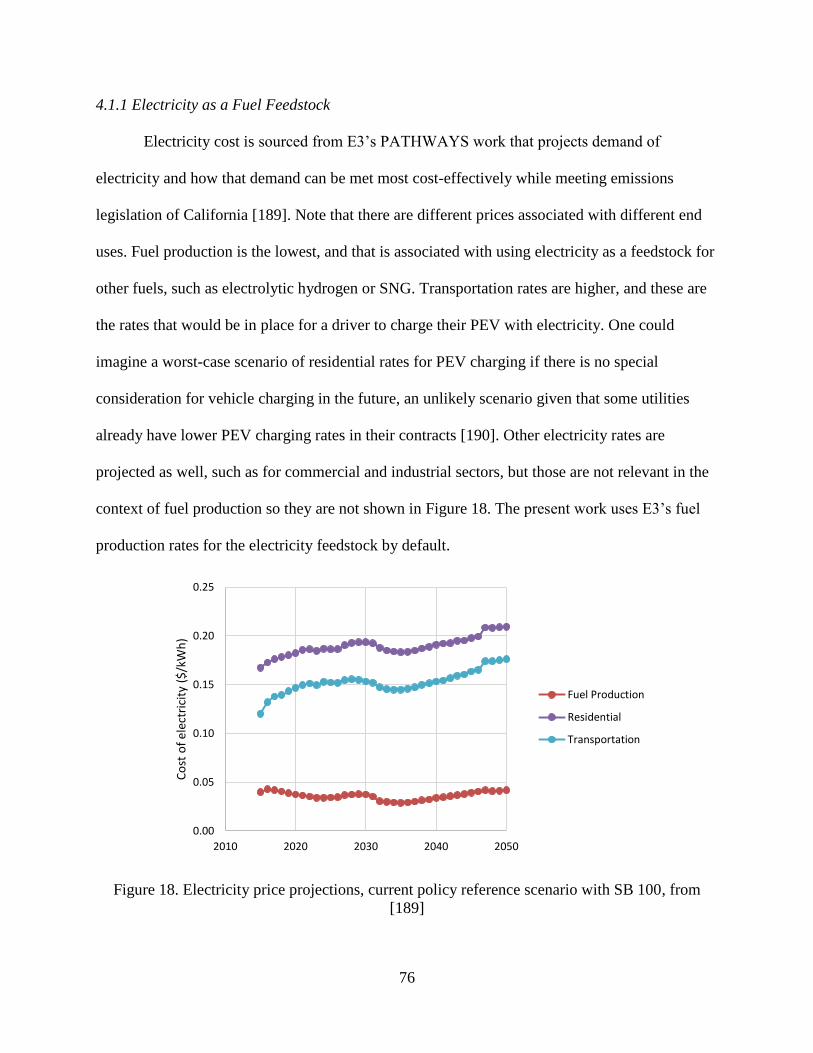
76

4.1.1 Electricity as a Fuel Feedstock

Electricity cost is sourced from E3’s PATHWAYS work that projects demand of

electricity and how that demand can be met most cost-effectively while meeting emissions

legislation of California [189]. Note that there are different prices associated with different end

uses. Fuel production is the lowest, and that is associated with using electricity as a feedstock for

other fuels, such as electrolytic hydrogen or SNG. Transportation rates are higher, and these are

the rates that would be in place for a driver to charge their PEV with electricity. One could

imagine a worst-case scenario of residential rates for PEV charging if there is no special

consideration for vehicle charging in the future, an unlikely scenario given that some utilities

already have lower PEV charging rates in their contracts [190]. Other electricity rates are

projected as well, such as for commercial and industrial sectors, but those are not relevant in the

context of fuel production so they are not shown in Figure 18. The present work uses E3’s fuel

production rates for the electricity feedstock by default.

Figure 18. Electricity price projections, current policy reference scenario with SB 100, from

[189]

0.00

0.05

0.10

0.15

0.20

0.25

2010 2020 2030 2040 2050

Co

st o

f el

ectr

icit

y ($

/kW

h)

Fuel Production

Residential

Transportation

77

These prices are assumed to be constant over the range of availabilities described in

Chapter 6.4, an assumption that is most accurate if the modeled electricity demand of this work

is similar to that of E3’s. Given the assumptions of Chapter 6.4, these prices should be

appropriate.

A co-feedstock one must consider with electrolytic fuels is water, as water is split to

produce hydrogen and oxygen. Water can come from various sources, and it is scarcer in

Southern California than Northern California. The Metropolitan Water District of Southern

California lists water rates for water originating from Northern California at around $300 per

acre-foot [191]. Using an average value from electricity costs of $0.0375/kWh, this leads to

water accounting for on the order of 0.1% of total electrolytic fuel production (this involves data

and calculations that are shortly to be detailed). Even at the extreme case of water produced by

desalination, with the highest cost estimates of $5,000 per acre-foot [192], that leads to water

costs of about 1.5% of total electrolytic fuel cost. Therefore, it is safe to assume water costs are

insignificant for these electrolytic fuels, and water is not analyzed in the proceeding techno-

economic work.

4.1.2 Biomass as a Fuel Feedstock

Prices for biomass feedstocks are found in the U.S. Department of Energy’s Billion Ton

Report [31]. Figure 19 shows the quantity of each of the categories of biomass available at

various selling prices. These quantities are given every 5 years from 2020 to 2040. Selling prices

start at $30/dry ton and increase by $10/dry ton increments up to $100/dry ton.

78

Figure 19. Current and potential biomass production for energy use in California based on

medium housing, medium energy use, and base case energy crop growth scenario with non-

organic MSW removed, data from [31].

Here, a weighted average of heating value for the categories of food waste, manure,

agriculture, waste, forestry, and energy crops is used to convert from dry ton of each individual

biomass feedstock to energy content. Weighting is based on the capacity available according to

the Billion Ton Report. Using the weighted average is justifiable for this conversion because the

relative ratio of the specific biomass feedstocks within the above categories stays relatively

similar throughout the years and prices considered, as shown in Figure 20.

0.0E+00

2.0E+07

4.0E+07

6.0E+07

8.0E+07

1.0E+08

1.2E+08

1.4E+08

30

50

70

90

30

50

70

90

30

50

70

90

30

50

70

90

30

50

70

90

2020 2025 2030 2035 2040

Sum

of

bio

mas

s fe

edst

ock

en

ergy

(G

J/yr

)

Ag Residues

Energy

Food Waste

Forest Residues

Manure

MSW

Tree

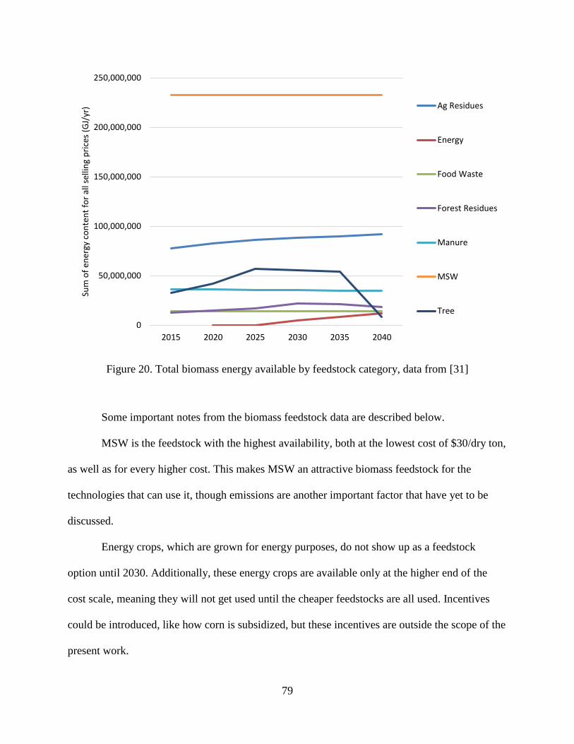
79

Figure 20. Total biomass energy available by feedstock category, data from [31]

Some important notes from the biomass feedstock data are described below.

MSW is the feedstock with the highest availability, both at the lowest cost of $30/dry ton,

as well as for every higher cost. This makes MSW an attractive biomass feedstock for the

technologies that can use it, though emissions are another important factor that have yet to be

discussed.

Energy crops, which are grown for energy purposes, do not show up as a feedstock

option until 2030. Additionally, these energy crops are available only at the higher end of the

cost scale, meaning they will not get used until the cheaper feedstocks are all used. Incentives

could be introduced, like how corn is subsidized, but these incentives are outside the scope of the

present work.

0

50,000,000

100,000,000

150,000,000

200,000,000

250,000,000

2015 2020 2025 2030 2035 2040

Sum

of

ener

gy c

on

ten

t fo

r al

l sel

ling

pri

ces

(GJ/

yr) Ag Residues

Energy

Food Waste

Forest Residues

Manure

MSW

Tree

80

Tree biomass reaches a peak in 2025, slightly declines until 2035, and then dramatically

reduces in 2040. One possible explanation for this is over-using this biomass in the earlier years

and reduced forestation in future years, leading to less dead and fallen trees for use as a

feedstock. This is an issue that should be further investigated to ensure sustainable use of this

biomass feedstock.

Lastly, some feedstocks have similar availabilities at all selling prices, while others have

increasing availability as selling price increases. Crop types that do not increase in availability

with selling price are food waste, forest residues, and manure. Crop types that do increase in

availability with selling price are agriculture residues, energy crops, MSW, and trees. This

behavior of increasing availability with selling price is indicative of the fact that increasing

selling price opens the opportunity for more involved and costly extraction or collection

procedures. For energy crops, which are expressly grown for energy uses, there is the additional

factor that increasing selling price increases the number of market players willing to grow energy

crops for profit. For the crop types that exhibit increased availability at increased selling price,

all but energy crops increase in availability for the first two selling price increases, but thereafter

stay constant in availability (or nearly constant in the case of agriculture residues). Energy crops

have a more consistent increase in availability at increasing selling price, likely due to the above-

mentioned factor of increasing market players.

Simplifications are made to reduce the number of separate cost brackets for each of the

feedstocks. For example, agriculture residues are available at $30/dry ton up to $100/dry ton at

different quantities for each $10/dry ton increment. However, looking at Figure 19, a reasonable

simplification is to consider in 2020 that 5.8e7 GJ/yr of agriculture residues available for $30/dry

ton, and 8e7 GJ/yr available for $50/dry ton. This is neglecting the slight increase in availability

81

at $40/dry ton compared to $30/dry ton, and the slight increase in availability at prices higher

than $50/dry ton. This same methodology is carried out for the rest of the years analyzed as well

as the other feedstocks with varying availabilities at different costs.

4.2 Fuel Production

This section details the efficiency and cost of fuel production for the five fuels considered

in this work (electricity, hydrogen, SNG, renewable gasoline, and renewable diesel). Note that

the electrolysis pathways for both hydrogen and SNG include the most detail as this was the area

with least information and agreement in the literature. The methodology developed for these

electrolytic fuels is then applied to the other fuel production methods.

Many methods have been proposed for estimating technological progress and the effects

on cost. These include Moore’s law [193], Wright’s law [194], and various other variants [195].

Nagy et al. tested these different methods for estimating technological progress based on a

database of 62 different technologies and showed that Wright’s law and Moore’s law perform

essentially the same with a slightly better performance by Wright’s law [195].

Wright’s law projects future capital costs based on the cumulative capacity produced

(rather than using time as in the case of Moore’s law). The equation for Wright’s law can be

written as shown in Equation 6 according to [196].

Equation 6. Wright's law

C(pt) = C(pi) (ptpi)−b

Here, pi is the initial production volume, pt is the production volume at time t, C(pt) is the

cost at production volume at time t, C(pi) is the cost at the initial production volume, and b is an

exponential learning parameter related to the learning rate (LR) by the equation.

82

Equation 7. Learning rate

LR = 1 − 2−b

Figure 21 shows the probability distribution of learning rates for various industrial technologies

collected from 108 studies [196].

Figure 21. Probability distribution of 108 studies that report learning rates in 22 industrial sectors

from [196]

In the coming sections, it will be shown that there is a wide range of current costs and

cost projections for electrolyzer technologies. Therefore, a conservative and an optimistic

scenario are proposed in this work for the cost projections of P2G equipment. The conservative

scenario assumes a constant 14% learning rate for electrolyzers and 10% for the remaining P2G

equipment throughout the timeframe considered. The optimistic scenario assumes a 25%

learning rate until 2030, 15% learning rate until 2035, and then 10% learning rate until 2050 for

the electrolyzers and a constant 14% learning rate for remaining P2G equipment. The rest of the

equipment considered in this work are less technologically-complicated and therefore have lower

83

associated learning rates because costs should not be expected to decrease as drastically.

Therefore, a learning rate of 10% is applied for non-P2G fuel production equipment.

Fuel production equipment has a dependence on scale for both efficiency and cost.

Therefore, for each type of equipment, the scale of plant used for the techno-economic data

presented is noted. Significant deviation in plant size from that scale could result in inaccuracies.

Generally, electrolyzers are less affected by scale than other fuel production equipment [197].

Note that while the following sections include cumulative installed capacities for each of

the fuel production technologies (in cumulative GW in the corresponding years shown), these

numbers should only be considered hypothetical examples at this point to give an idea of how

cumulative installed capacities of these technologies affect cost. The capacities shown will be

further detailed in Chapter 6, and the actual projected cumulative installed capacities of the

modeling will be determined by a methodology explained in Chapter 7.

4.2.1 Hydrogen Fuel Production

Hydrogen can be produced by electrolysis or gasification in the context of this work.

Both the electrolyzers and gasifiers are taken to be 50 MW in size.

4.2.1.1 Electrolytic Hydrogen Fuel Production

Electrolytic hydrogen uses electricity as its feedstock and electrolyzers as the fuel

production equipment. As noted before, water costs are negligible and will therefore not be

considered in the proceeding work.

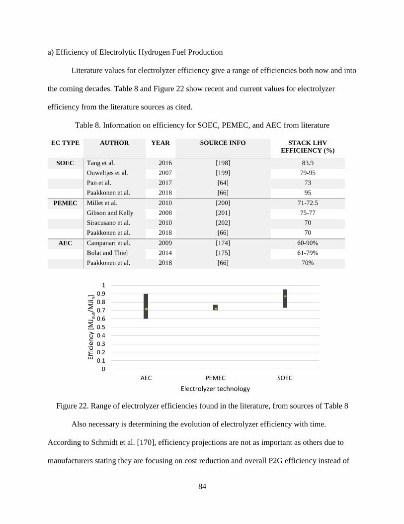
84

a) Efficiency of Electrolytic Hydrogen Fuel Production

Literature values for electrolyzer efficiency give a range of efficiencies both now and into

the coming decades. Table 8 and Figure 22 show recent and current values for electrolyzer

efficiency from the literature sources as cited.

Table 8. Information on efficiency for SOEC, PEMEC, and AEC from literature

EC TYPE AUTHOR YEAR SOURCE INFO STACK LHV

EFFICIENCY (%)

SOEC Tang et al. 2016 [198] 83.9

Ouweltjes et al. 2007 [199] 79-95

Pan et al. 2017 [64] 73

Paakkonen et al. 2018 [66] 95

PEMEC Millet et al. 2010 [200] 71-72.5

Gibson and Kelly 2008 [201] 75-77

Siracusano et al. 2010 [202] 70

Paakkonen et al. 2018 [66] 70

AEC Campanari et al. 2009 [174] 60-90%

Bolat and Thiel 2014 [175] 61-79%

Paakkonen et al. 2018 [66] 70%

Figure 22. Range of electrolyzer efficiencies found in the literature, from sources of Table 8

Also necessary is determining the evolution of electrolyzer efficiency with time.

According to Schmidt et al. [170], efficiency projections are not as important as others due to

manufacturers stating they are focusing on cost reduction and overall P2G efficiency instead of

0

0.1

0.2

0.3

0.4

0.5

0.6

0.7

0.8

0.9

1

AEC PEMEC SOEC

Effi

cien

cy [

MJ o

ut/

MJi

n]

Electrolyzer technology

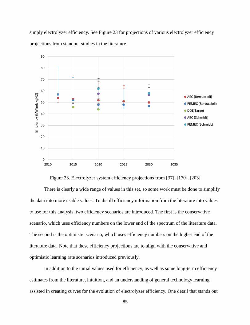
85

simply electrolyzer efficiency. See Figure 23 for projections of various electrolyzer efficiency

projections from standout studies in the literature.

Figure 23. Electrolyzer system efficiency projections from [37], [170], [203]

There is clearly a wide range of values in this set, so some work must be done to simplify

the data into more usable values. To distill efficiency information from the literature into values

to use for this analysis, two efficiency scenarios are introduced. The first is the conservative

scenario, which uses efficiency numbers on the lower end of the spectrum of the literature data.

The second is the optimistic scenario, which uses efficiency numbers on the higher end of the

literature data. Note that these efficiency projections are to align with the conservative and

optimistic learning rate scenarios introduced previously.

In addition to the initial values used for efficiency, as well as some long-term efficiency

estimates from the literature, intuition, and an understanding of general technology learning

assisted in creating curves for the evolution of electrolyzer efficiency. One detail that stands out

0

10

20

30

40

50

60

70

80

90

2010 2015 2020 2025 2030 2035

Effi

cien

cy (

kWh

el/k

gH2

)

AEC (Bertuccioli)

PEMEC (Bertuccioli)

DOE Target

AEC (Schmidt)

PEMEC (Schmidt)

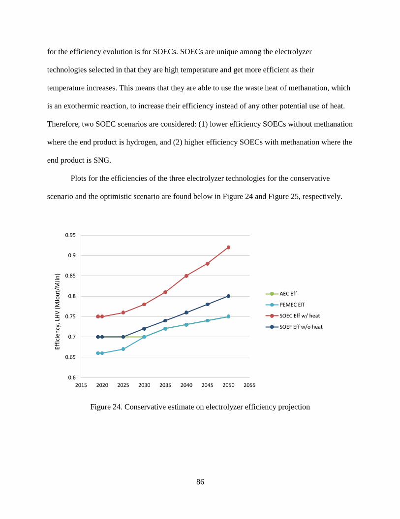
86

for the efficiency evolution is for SOECs. SOECs are unique among the electrolyzer

technologies selected in that they are high temperature and get more efficient as their

temperature increases. This means that they are able to use the waste heat of methanation, which

is an exothermic reaction, to increase their efficiency instead of any other potential use of heat.

Therefore, two SOEC scenarios are considered: (1) lower efficiency SOECs without methanation

where the end product is hydrogen, and (2) higher efficiency SOECs with methanation where the

end product is SNG.

Plots for the efficiencies of the three electrolyzer technologies for the conservative

scenario and the optimistic scenario are found below in Figure 24 and Figure 25, respectively.

Figure 24. Conservative estimate on electrolyzer efficiency projection

0.6

0.65

0.7

0.75

0.8

0.85

0.9

0.95

2015 2020 2025 2030 2035 2040 2045 2050 2055

Effi

cien

cy, L

HV

(M

Jou

t/M

Jin

)

AEC Eff

PEMEC Eff

SOEC Eff w/ heat

SOEF Eff w/o heat

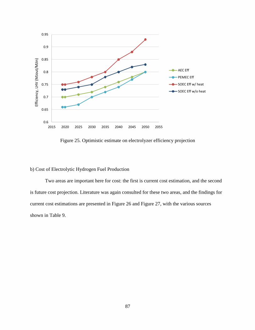
87

Figure 25. Optimistic estimate on electrolyzer efficiency projection

b) Cost of Electrolytic Hydrogen Fuel Production

Two areas are important here for cost: the first is current cost estimation, and the second

is future cost projection. Literature was again consulted for these two areas, and the findings for

current cost estimations are presented in Figure 26 and Figure 27, with the various sources

shown in Table 9.

0.6

0.65

0.7

0.75

0.8

0.85

0.9

0.95

2015 2020 2025 2030 2035 2040 2045 2050 2055

Effi

cien

cy, L

HV

(M

Jou

t/M

Jin

)

AEC Eff

PEMEC Eff

SOEC Eff w/ heat

SOEC Eff w/o heat

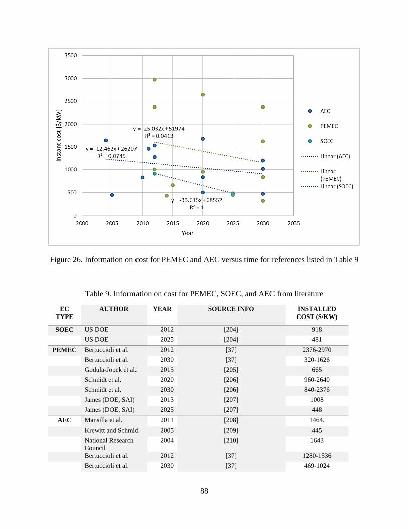
88

Figure 26. Information on cost for PEMEC and AEC versus time for references listed in Table 9

Table 9. Information on cost for PEMEC, SOEC, and AEC from literature

EC

TYPE

AUTHOR YEAR SOURCE INFO INSTALLED

COST ($/KW)

SOEC US DOE 2012 [204] 918

US DOE 2025 [204] 481

PEMEC Bertuccioli et al. 2012 [37] 2376-2970

Bertuccioli et al. 2030 [37] 320-1626

Godula-Jopek et al. 2015 [205] 665

Schmidt et al. 2020 [206] 960-2640

Schmidt et al. 2030 [206] 840-2376

James (DOE, SAI) 2013 [207] 1008

James (DOE, SAI) 2025 [207] 448

AEC Mansilla et al. 2011 [208] 1464.

Krewitt and Schmid 2005 [209] 445

National Research

Council

2004 [210] 1643



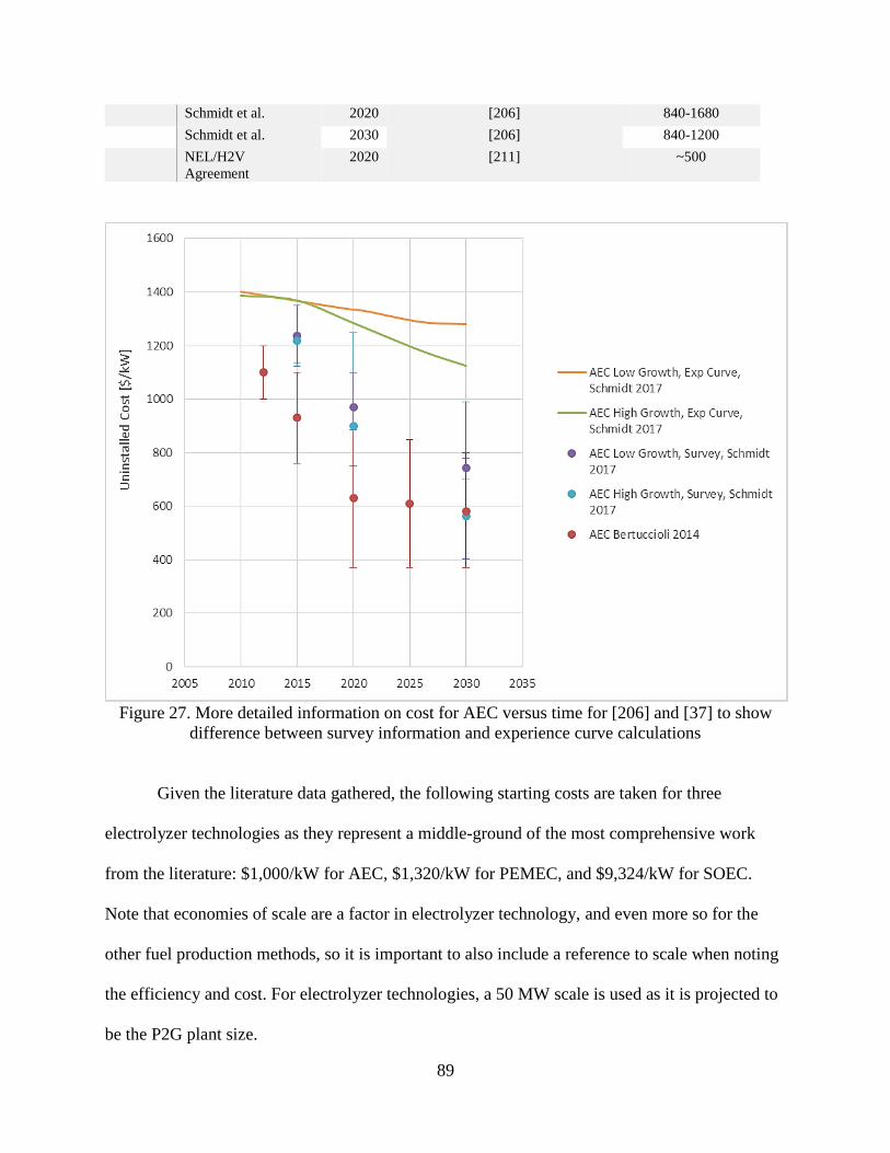
89

Schmidt et al. 2020 [206] 840-1680

Schmidt et al. 2030 [206] 840-1200

NEL/H2V

Agreement

2020 [211] ~500

Figure 27. More detailed information on cost for AEC versus time for [206] and [37] to show

difference between survey information and experience curve calculations

Given the literature data gathered, the following starting costs are taken for three

electrolyzer technologies as they represent a middle-ground of the most comprehensive work

from the literature: $1,000/kW for AEC, $1,320/kW for PEMEC, and $9,324/kW for SOEC.

Note that economies of scale are a factor in electrolyzer technology, and even more so for the

other fuel production methods, so it is important to also include a reference to scale when noting

the efficiency and cost. For electrolyzer technologies, a 50 MW scale is used as it is projected to

be the P2G plant size.

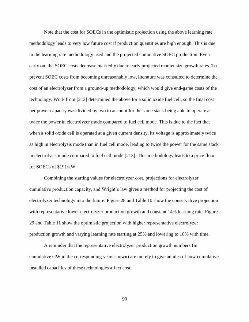
90

Note that the cost for SOECs in the optimistic projection using the above learning rate

methodology leads to very low future cost if production quantities are high enough. This is due

to the learning rate methodology used and the projected cumulative SOEC production. Even

early on, the SOEC costs decrease markedly due to early projected market size growth rates. To

prevent SOEC costs from becoming unreasonably low, literature was consulted to determine the

cost of an electrolyzer from a ground-up methodology, which would give end-game costs of the

technology. Work from [212] determined the above for a solid oxide fuel cell, so the final cost

per power capacity was divided by two to account for the same stack being able to operate at

twice the power in electrolyzer mode compared to fuel cell mode. This is due to the fact that

when a solid oxide cell is operated at a given current density, its voltage is approximately twice

as high in electrolysis mode than in fuel cell mode, leading to twice the power for the same stack

in electrolysis mode compared to fuel cell mode [213]. This methodology leads to a price floor

for SOECs of $191/kW.

Combining the starting values for electrolyzer cost, projections for electrolyzer

cumulative production capacity, and Wright’s law gives a method for projecting the cost of

electrolyzer technology into the future. Figure 28 and Table 10 show the conservative projection

with representative lower electrolyzer production growth and constant 14% learning rate. Figure

29 and Table 11 show the optimistic projection with higher representative electrolyzer

production growth and varying learning rate starting at 25% and lowering to 10% with time.

A reminder that the representative electrolyzer production growth numbers (in

cumulative GW in the corresponding years shown) are merely to give an idea of how cumulative

installed capacities of these technologies affect cost.

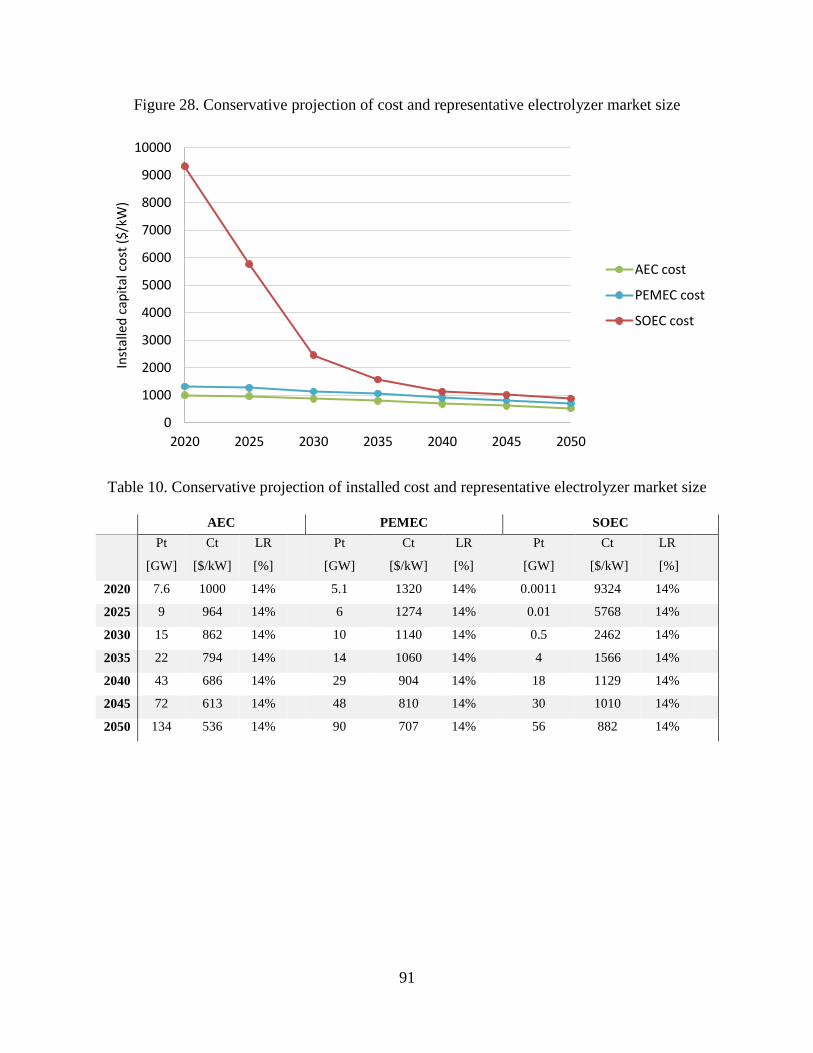
91

Figure 28. Conservative projection of cost and representative electrolyzer market size

Table 10. Conservative projection of installed cost and representative electrolyzer market size

AEC PEMEC SOEC

Pt

[GW]

Ct

[$/kW]

LR

[%]

Pt

[GW]

Ct

[$/kW]

LR

[%]

Pt

[GW]

Ct

[$/kW]

LR

[%]

2020 7.6 1000 14% 5.1 1320 14% 0.0011 9324 14%

2025 9 964 14% 6 1274 14% 0.01 5768 14%

2030 15 862 14% 10 1140 14% 0.5 2462 14%

2035 22 794 14% 14 1060 14% 4 1566 14%

2040 43 686 14% 29 904 14% 18 1129 14%

2045 72 613 14% 48 810 14% 30 1010 14%

2050 134 536 14% 90 707 14% 56 882 14%

0

1000

2000

3000

4000

5000

6000

7000

8000

9000

10000

2020 2025 2030 2035 2040 2045 2050

Inst

alle

d c

apit

al c

ost

($

/kW

)

AEC cost

PEMEC cost

SOEC cost

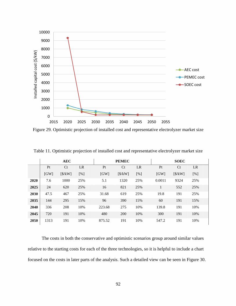
92

Figure 29. Optimistic projection of installed cost and representative electrolyzer market size

Table 11. Optimistic projection of installed cost and representative electrolyzer market size

AEC PEMEC SOEC

Pt

[GW]

Ct

[$/kW]

LR

[%]

Pt

[GW]

Ct

[$/kW]

LR

[%]

Pt

[GW]

Ct

[$/kW]

LR

[%]

2020 7.6 1000 25% 5.1 1320 25% 0.0011 9324 25%

2025 24 620 25% 16 821 25% 1 552 25%

2030 47.5 467 25% 31.68 619 25% 19.8 191 25%

2035 144 295 15% 96 390 15% 60 191 15%

2040 336 208 10% 223.68 275 10% 139.8 191 10%

2045 720 191 10% 480 200 10% 300 191 10%

2050 1313 191 10% 875.52 191 10% 547.2 191 10%

The costs in both the conservative and optimistic scenarios group around similar values

relative to the starting costs for each of the three technologies, so it is helpful to include a chart

focused on the costs in later parts of the analysis. Such a detailed view can be seen in Figure 30.

0

1000

2000

3000

4000

5000

6000

7000

8000

9000

10000

2015 2020 2025 2030 2035 2040 2045 2050 2055

Inst

alle

d c

apit

al c

ost

($

/kW

)

AEC cost

PEMEC cost

SOEC cost

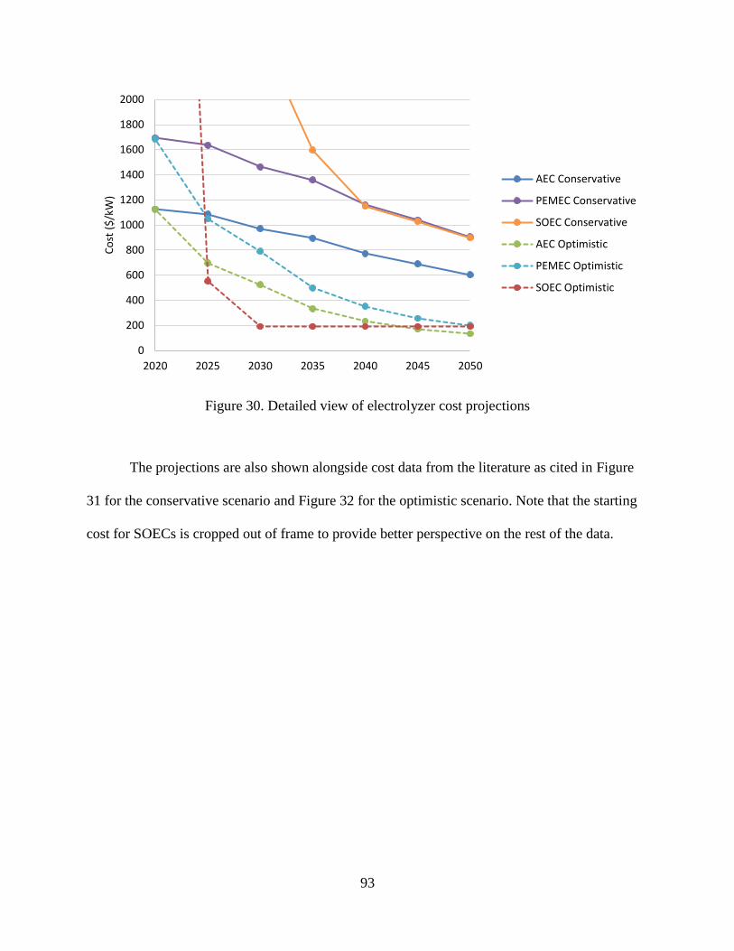
93

Figure 30. Detailed view of electrolyzer cost projections

The projections are also shown alongside cost data from the literature as cited in Figure

31 for the conservative scenario and Figure 32 for the optimistic scenario. Note that the starting

cost for SOECs is cropped out of frame to provide better perspective on the rest of the data.

0

200

400

600

800

1000

1200

1400

1600

1800

2000

2020 2025 2030 2035 2040 2045 2050

Co

st (

$/k

W)

AEC Conservative

PEMEC Conservative

SOEC Conservative

AEC Optimistic

PEMEC Optimistic

SOEC Optimistic

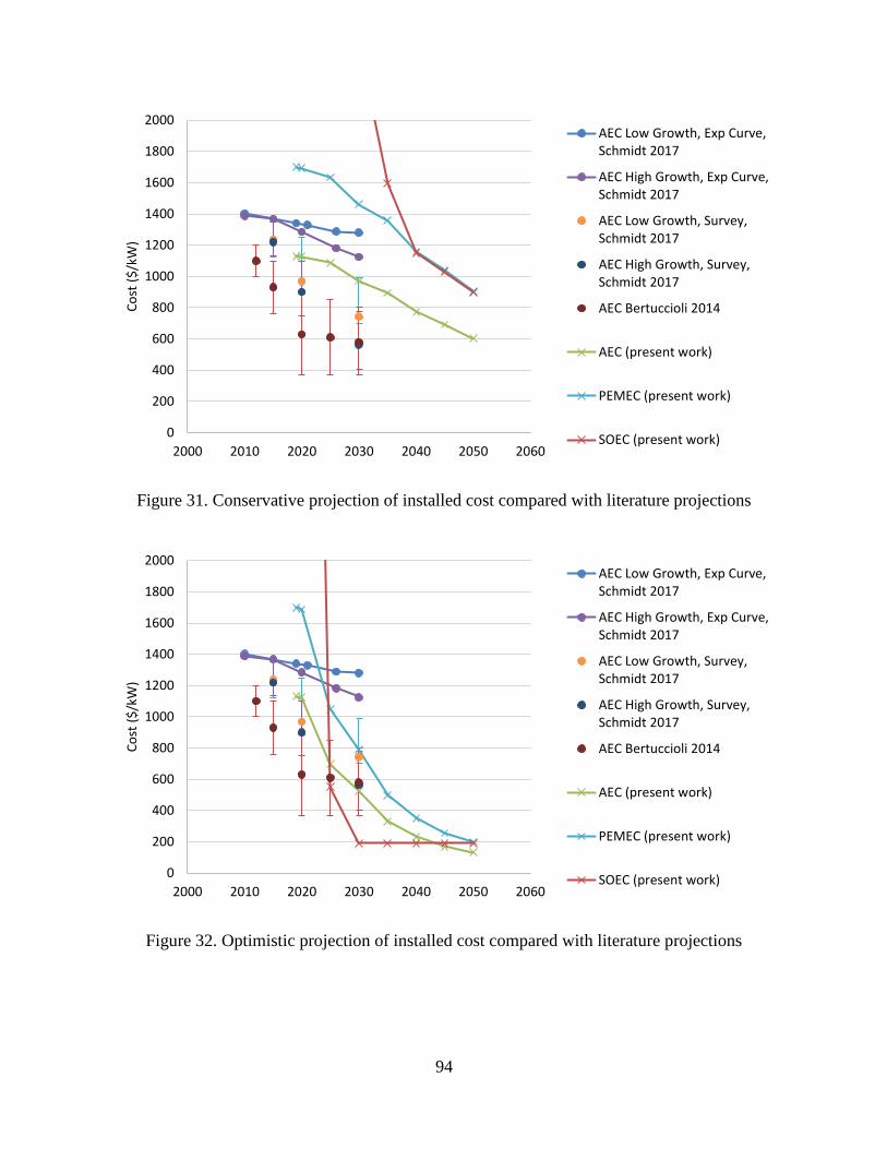
94

Figure 31. Conservative projection of installed cost compared with literature projections

Figure 32. Optimistic projection of installed cost compared with literature projections

0

200

400

600

800

1000

1200

1400

1600

1800

2000

2000 2010 2020 2030 2040 2050 2060

Co

st (

$/k

W)

AEC Low Growth, Exp Curve,Schmidt 2017

AEC High Growth, Exp Curve,Schmidt 2017

AEC Low Growth, Survey,Schmidt 2017

AEC High Growth, Survey,Schmidt 2017

AEC Bertuccioli 2014

AEC (present work)

PEMEC (present work)

SOEC (present work)

0

200

400

600

800

1000

1200

1400

1600

1800

2000

2000 2010 2020 2030 2040 2050 2060

Co

st (

$/k

W)

AEC Low Growth, Exp Curve,Schmidt 2017

AEC High Growth, Exp Curve,Schmidt 2017

AEC Low Growth, Survey,Schmidt 2017

AEC High Growth, Survey,Schmidt 2017

AEC Bertuccioli 2014

AEC (present work)

PEMEC (present work)

SOEC (present work)

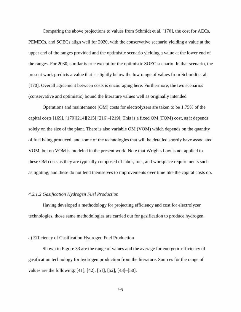
95

Comparing the above projections to values from Schmidt et al. [170], the cost for AECs,

PEMECs, and SOECs align well for 2020, with the conservative scenario yielding a value at the

upper end of the ranges provided and the optimistic scenario yielding a value at the lower end of

the ranges. For 2030, similar is true except for the optimistic SOEC scenario. In that scenario, the

present work predicts a value that is slightly below the low range of values from Schmidt et al.

[170]. Overall agreement between costs is encouraging here. Furthermore, the two scenarios

(conservative and optimistic) bound the literature values well as originally intended.

Operations and maintenance (OM) costs for electrolyzers are taken to be 1.75% of the

capital costs [169], [170][214][215] [216]–[219]. This is a fixed OM (FOM) cost, as it depends

solely on the size of the plant. There is also variable OM (VOM) which depends on the quantity

of fuel being produced, and some of the technologies that will be detailed shortly have associated

VOM, but no VOM is modeled in the present work. Note that Wrights Law is not applied to

these OM costs as they are typically composed of labor, fuel, and workplace requirements such

as lighting, and these do not lend themselves to improvements over time like the capital costs do.

4.2.1.2 Gasification Hydrogen Fuel Production

Having developed a methodology for projecting efficiency and cost for electrolyzer

technologies, those same methodologies are carried out for gasification to produce hydrogen.

a) Efficiency of Gasification Hydrogen Fuel Production

Shown in Figure 33 are the range of values and the average for energetic efficiency of

gasification technology for hydrogen production from the literature. Sources for the range of

values are the following: [41], [42], [51], [52], [43]–[50].

96

Figure 33. Gasification efficiency ranges and average for hydrogen production, data from [41],

[42], [51], [52], [43]–[50]

The method used for projecting gasification efficiency for hydrogen production is to start

with the average literature value of 0.54 in 2020 and reach the high efficiency estimates by 2050.

Progress is assumed to be about half by 2035. The modeled efficiency projections are shown in

Figure 34.

Figure 34. Efficiency projections of gasification for hydrogen production

0.0

0.1

0.2

0.3

0.4

0.5

0.6

0.7

0.8

H2Ef

fici

ency

0

0.1

0.2

0.3

0.4

0.5

0.6

0.7

0.8

2015 2020 2025 2030 2035 2040 2045 2050 2055

LHV

Eff

icie

ncy

(-)

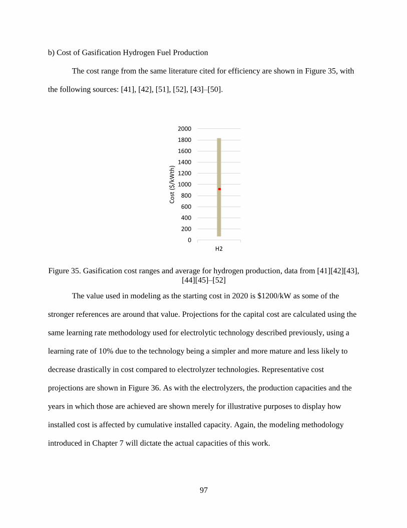
97

b) Cost of Gasification Hydrogen Fuel Production

The cost range from the same literature cited for efficiency are shown in Figure 35, with

the following sources: [41], [42], [51], [52], [43]–[50].

Figure 35. Gasification cost ranges and average for hydrogen production, data from [41][42][43],

[44][45]–[52]

The value used in modeling as the starting cost in 2020 is $1200/kW as some of the

stronger references are around that value. Projections for the capital cost are calculated using the

same learning rate methodology used for electrolytic technology described previously, using a

learning rate of 10% due to the technology being a simpler and more mature and less likely to

decrease drastically in cost compared to electrolyzer technologies. Representative cost

projections are shown in Figure 36. As with the electrolyzers, the production capacities and the

years in which those are achieved are shown merely for illustrative purposes to display how

installed cost is affected by cumulative installed capacity. Again, the modeling methodology

introduced in Chapter 7 will dictate the actual capacities of this work.

0

200

400

600

800

1000

1200

1400

1600

1800

2000

H2

Co

st (

$/k

Wth

)

98

Figure 36. Cost projection for gasification production of hydrogen

FOM is estimated as $40/kW-yr and VOM is estimated as $6/kWh, using the same

literature sources from which the capital costs are sourced [41][42][43], [44][45]–[52].

4.2.2 SNG Fuel Production

SNG can start much in the same way as hydrogen, but with the additional step of

methanation. The required data for hydrogen are the same as electrolytic hydrogen production as

previously detailed. The following is for the methanation requirement, which would be added on

top of the electrolytic hydrogen production. SNG can also be made through AD and gasification.

SNG produced by electrolyzers (and the accompanying methanation equipment) and

gasifiers are by plants of the scale of 50 MW. The AD plant is smaller, on the order of 500 kW.

0

200

400

600

800

1000

1200

0

200

400

600

800

1000

1200

1400

2020 2025 2030 2035 2040 2045 2050

Cu

mu

lati

ve in

stal

led

cap

acit

y (G

W)

Inst

alle

d c

ost

($

/kW

th)

Installed cost ($/kWth)

Cumulative GW

99

4.2.2.1 Electrolytic SNG Fuel Production

a) Efficiency of Electrolytic SNG Fuel Production

Methanation efficiency is 79% as calculated previously in the Electrolytic SNG section of

the Background. The efficiency drop for the carbon capture technology is neglected as the power

requirement is small compared to that of the electrolyzer. Therefore, the overall efficiency of

converting the electrolytic hydrogen to SNG is 79%.

b) Cost of Electrolytic SNG Fuel Production

Previous work has shown that due to the production costs, electrolytic SNG is not

economical for plants with low capacity factors, or utilization compared to nameplate capacity

[63]. The present work will provide more insight into this area with a detailed techno-economic

analysis as an input to the overall optimization.

The supporting P2G equipment cost is determined using the same learning rate

methodology as for the electrolyzers. For these technologies, the learning rate is assumed to be

10% for the conservative scenario and 14% for the optimistic scenario as previously noted.

Methanator

In Table 12, the installed methanator capacities shown are determined by the capacity

required for methane production corresponding to the installed electrolyzer capacity (which

again is merely a hypothetical example to illustrate the dependence of cost on production).

Capacities are given as GW of SNG output.

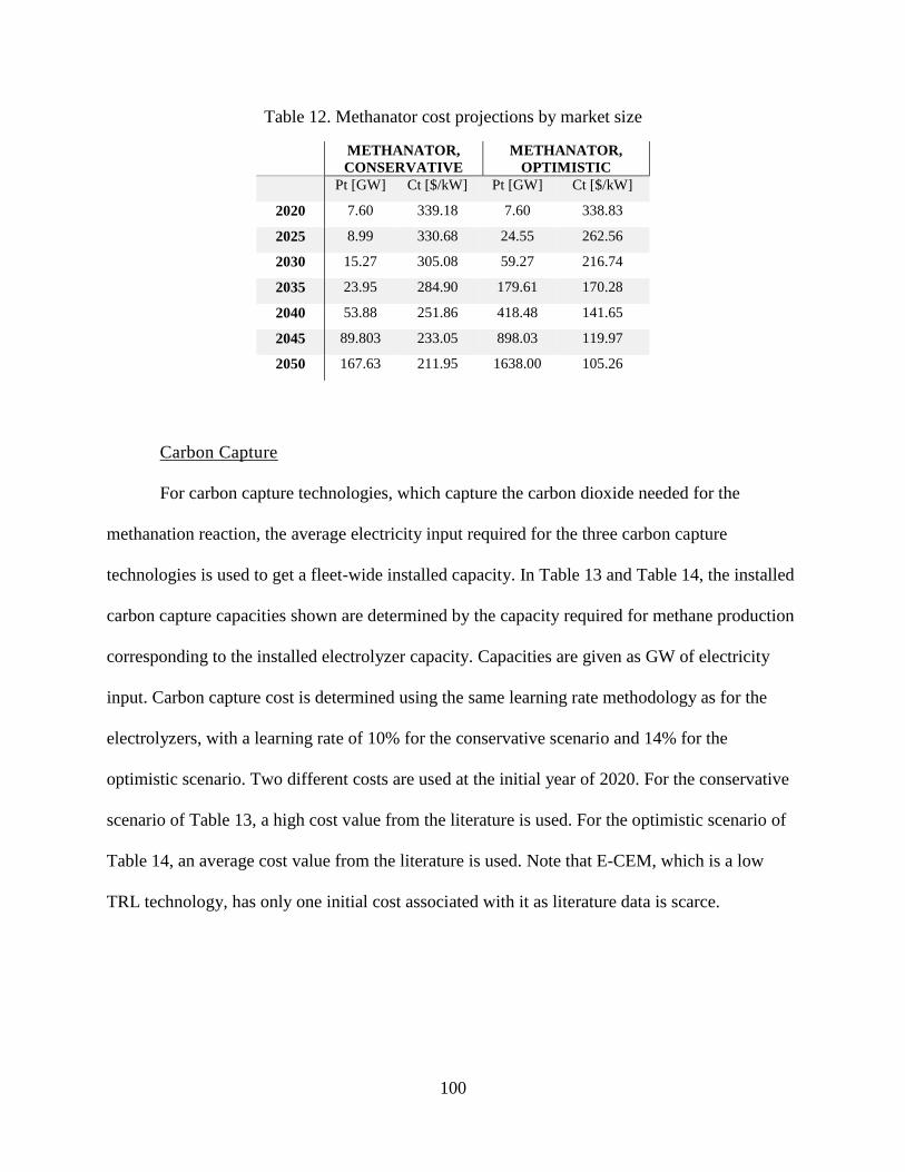
100

Table 12. Methanator cost projections by market size

METHANATOR,

CONSERVATIVE

METHANATOR,

OPTIMISTIC

Pt [GW] Ct [$/kW] Pt [GW] Ct [$/kW]

2020 7.60 339.18 7.60 338.83

2025 8.99 330.68 24.55 262.56

2030 15.27 305.08 59.27 216.74

2035 23.95 284.90 179.61 170.28

2040 53.88 251.86 418.48 141.65

2045 89.803 233.05 898.03 119.97

2050 167.63 211.95 1638.00 105.26

Carbon Capture

For carbon capture technologies, which capture the carbon dioxide needed for the

methanation reaction, the average electricity input required for the three carbon capture

technologies is used to get a fleet-wide installed capacity. In Table 13 and Table 14, the installed

carbon capture capacities shown are determined by the capacity required for methane production

corresponding to the installed electrolyzer capacity. Capacities are given as GW of electricity

input. Carbon capture cost is determined using the same learning rate methodology as for the

electrolyzers, with a learning rate of 10% for the conservative scenario and 14% for the

optimistic scenario. Two different costs are used at the initial year of 2020. For the conservative

scenario of Table 13, a high cost value from the literature is used. For the optimistic scenario of

Table 14, an average cost value from the literature is used. Note that E-CEM, which is a low

TRL technology, has only one initial cost associated with it as literature data is scarce.

101

Table 13. Conservative projection of carbon capture technology cost by market size

E-CEM, CONSERVATIVE PCC, CONSERVATIVE DAC, CONSERVATIVE

Pt [GW] Ct [$/tonCO2/d] Pt [GW] Ct [$/tonCO2/d] Pt [GW] Ct [$/tonCO2/d]

2020 0.2238 1.82E+06 0.2238 6.35E+04 0.2238 4.55E+05

2025 0.2645 1.77E+06 0.2645 6.19E+04 0.2645 4.44E+05

2030 0.4493 1.63E+06 0.4493 5.71E+04 0.4493 4.09E+05

2035 0.7048 1.53E+06 0.7048 5.33E+04 0.7048 3.82E+05

2040 1.5859 1.35E+06 1.5859 4.71E+04 1.5859 3.38E+05

2045 2.6432 1.25E+06 2.6432 4.36E+04 2.6432 3.13E+05

2050 4.9339 1.13E+06 4.9339 3.97E+04 4.9339 2.84E+05

Table 14. Optimistic projection of carbon capture technology cost by market size

E-CEM, OPTIMISTIC PCC, OPTIMISTIC DAC, OPTIMISTIC

Pt [GW] Ct [$/tonCO2/d] Pt [GW] Ct [$/tonCO2/d] Pt [GW] Ct [$/tonCO2/d]

2020 0.2238 1.81E+06 0.2238 4.36E+04 0.2238 3.15E+05

2025 0.7225 1.41E+06 0.7225 3.38E+04 0.7225 2.44E+05

2030 1.7445 1.16E+06 1.7445 2.79E+04 1.7445 2.01E+05

2035 5.2864 9.12E+05 5.2864 2.19E+04 5.2864 1.58E+05

2040 12.3173 7.58E+05 12.3173 1.82E+04 12.3173 1.32E+05

2045 26.4319 6.42E+05 26.4319 1.54E+04 26.4319 1.11E+05

2050 48.2117 5.64E+05 48.2117 1.35E+04 48.2117 9.77E+04

VOM for all scenarios, including the methanator, carbon capture source, and heat sink, is

$0.01/kWh. FOM is estimated as $200/kW-yr for E-CEM scenarios, $10/kW-yr for PCC

scenarios, and $8/kW-yr for DAC scenarios [72], [216], [220].

Co-locating a P2G plant with a biorefinery producing biofuels can be a particularly

attractive option both economically and environmentally. Economically, this concept would use

PCC technology, which is the lowest cost carbon capture technology as seen in Table 13 and

Table 14. Environmentally, this concept would use biomass feedstocks to produce either a

gaseous or liquid fuel in a bioconversion plant, in addition to carbon dioxide that can be added to

102

hydrogen to produce SNG. This would maximize the fuel potential and therefore energy

extraction of carbon that is stored in biomass.

While this co-location is attractive for the reasons stated above, it is important to note that

there are practical limitations that may hinder widespread adoption. A P2G plant must be fed by

off-grid solar or wind to economically make fuel in a carbon-free manner. Additionally,

electrolysis requires water input, so this P2G plant must also be at or near a large source of water

for economic and logistic reasons. Lastly, this P2G plant must also be located adjacent to a

biorefinery to get the carbon dioxide from that plant. This biorefinery would be best located near

a large source of biomass to improve efficiency, economics, and logistics of the biorefinery. One

can now see the many factors that must be aligned for a P2G plant co-located with a biorefinery

to come to fruition. Therefore, these combined plants should be considered an optimistic option

that should be pursued when possible, but not be assumed to be widely existent in the future.

Heat Sink

Steam turbine installed capacity is determined as the power output of the turbines that

would be required by the heat output of the methanator for the given scenario’s power input.

Costs are again determined using the learning rate methodology, with a learning rate of 10% for

the conservative scenario and 14% for the optimistic scenario.

Here, it is important to determine the size of steam turbine that would be expected to be

at a P2G plant. This is because the cost and efficiency of steam turbines vary based on scale.

Estimating P2G plants to be approximately 50 MW of electricity input [221] and using the heat

rejected from the methanator, we arrive at a steam turbine on the order of 3 MW, which is a

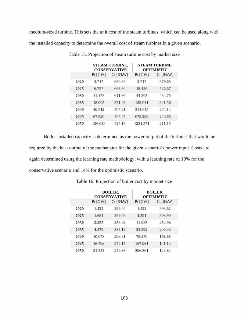
103

medium-sized turbine. This sets the unit cost of the steam turbines, which can be used along with

the installed capacity to determine the overall cost of steam turbines in a given scenario.

Table 15. Projection of steam turbine cost by market size

STEAM TURBINE,

CONSERVATIVE

STEAM TURBINE,

OPTIMISTIC


2020 5.717 680.36 5.717 679.65

2025 6.757 663.30 18.456 526.67

2030 11.478 611.96 44.563 434.75

2035 18.005 571.49 135.041 341.56

2040 40.512 505.21 314.645 284.14

2045 67.520 467.47 675.203 240.65

2050 126.038 425.16 1231.571 211.15

Boiler installed capacity is determined as the power output of the turbines that would be

required by the heat output of the methanator for the given scenario’s power input. Costs are

again determined using the learning rate methodology, with a learning rate of 10% for the

conservative scenario and 14% for the optimistic scenario.

Table 16. Projection of boiler cost by market size

BOILER,

CONSERVATIVE

BOILER,

OPTIMISTIC


2020 1.422 399.04 1.422 398.62

2025 1.681 389.03 4.591 308.90

2030 2.855 358.92 11.085 254.98

2035 4.479 335.18 33.592 200.33

2040 10.078 296.31 78.270 166.65

2045 16.796 274.17 167.961 141.14

2050 31.353 249.36 306.361 123.84

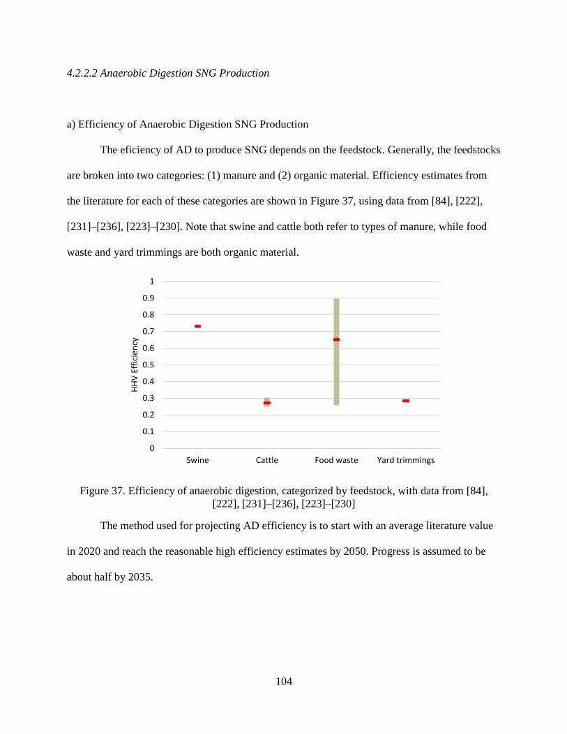
104

4.2.2.2 Anaerobic Digestion SNG Production

a) Efficiency of Anaerobic Digestion SNG Production

The eficiency of AD to produce SNG depends on the feedstock. Generally, the feedstocks

are broken into two categories: (1) manure and (2) organic material. Efficiency estimates from

the literature for each of these categories are shown in Figure 37, using data from [84], [222],

[231]–[236], [223]–[230]. Note that swine and cattle both refer to types of manure, while food

waste and yard trimmings are both organic material.

Figure 37. Efficiency of anaerobic digestion, categorized by feedstock, with data from [84],

[222], [231]–[236], [223]–[230]

The method used for projecting AD efficiency is to start with an average literature value

in 2020 and reach the reasonable high efficiency estimates by 2050. Progress is assumed to be

about half by 2035.

0

0.1

0.2

0.3

0.4

0.5

0.6

0.7

0.8

0.9

1

Swine Cattle Food waste Yard trimmings

HH

V E

ffic

ien

cy

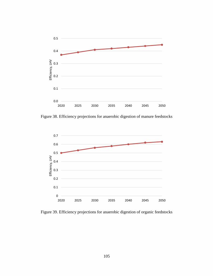
105

Figure 38. Efficiency projections for anaerobic digestion of manure feedstocks

Figure 39. Efficiency projections for anaerobic digestion of organic feedstocks

0.0

0.1

0.2

0.3

0.4

0.5

2020 2025 2030 2035 2040 2045 2050

Effi

cien

cy, L

HV

0

0.1

0.2

0.3

0.4

0.5

0.6

0.7

2020 2025 2030 2035 2040 2045 2050

Effi

cien

cy, L

HV

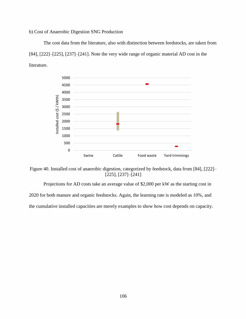
106

b) Cost of Anaerobic Digestion SNG Production

The cost data from the literature, also with distinction between feedstocks, are taken from

[84], [222]–[225], [237]–[241]. Note the very wide range of organic material AD cost in the

literature.

Figure 40. Installed cost of anaerobic digestion, categorized by feedstock, data from [84], [222]–

[225], [237]–[241]

Projections for AD costs take an average value of $2,000 per kW as the starting cost in

2020 for both manure and organic feedstocks. Again, the learning rate is modeled as 10%, and

the cumulative installed capacities are merely examples to show how cost depends on capacity.

0

500

1000

1500

2000

2500

3000

3500

4000

4500

5000

Swine Cattle Food waste Yard trimmings

Inst

alle

d c

ost

($

/ k

Wth

)

107

Figure 41. Cost projections for anaerobic digestion

FOM for AD is modeled as $60/kW-yr and $0.01/kWh [84], [222]–[225], [237]–[241].

4.2.2.3 Gasification SNG Production

a) Efficiency of Gasification SNG Production

Shown in Figure 42 are the range of values and the average for energetic efficiency of

gasification technology from the literature, specified by the fuel being produced. Sources for the

SNG production data are the following: [86], [87], [96]–[104], [88]–[95][105], [106], [115],

[116], [107]–[114]. The value used in modeling is 0.67. Again, a 50MW plant is used for design.

0

200

400

600

800

1000

1200

0.00

500.00

1000.00

1500.00

2000.00

2500.00

2020 2030 2040 2050

Cu

mu

lati

ve in

stal

led

cap

acit

y (G

Wth

)

Inst

alle

d c

ost

($

/kW

th)

$/kWth

Cumulative GWth

108

Figure 42. Gasification efficiency ranges and average for SNG production, data from [86], [87],

[96]–[104], [88]–[95][105], [106], [115], [116], [107]–[114].

The method used for projecting gasification efficiency for SNG production is to start with

the average literature value in 2020 and reach the reasonable high efficiency estimates by 2050.

Progress is assumed to be about half by 2035.

Figure 43. Efficiency projections for gasification for SNG production

0.0

0.1

0.2

0.3

0.4

0.5

0.6

0.7

0.8

0.9

SNGEf

fici

ency

0

0.1

0.2

0.3

0.4

0.5

0.6

0.7

0.8

2015 2020 2025 2030 2035 2040 2045 2050 2055

LHV

Eff

icie

ncy

(-)

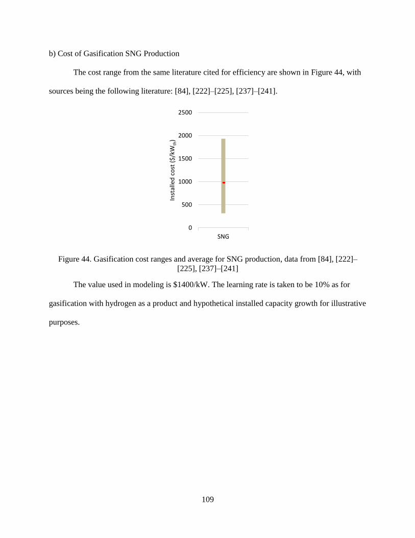
109

b) Cost of Gasification SNG Production

The cost range from the same literature cited for efficiency are shown in Figure 44, with

sources being the following literature: [84], [222]–[225], [237]–[241].

Figure 44. Gasification cost ranges and average for SNG production, data from [84], [222]–

[225], [237]–[241]

The value used in modeling is $1400/kW. The learning rate is taken to be 10% as for

gasification with hydrogen as a product and hypothetical installed capacity growth for illustrative

purposes.

0

500

1000

1500

2000

2500

SNG

Inst

alle

d c

ost

($

/kW

th)

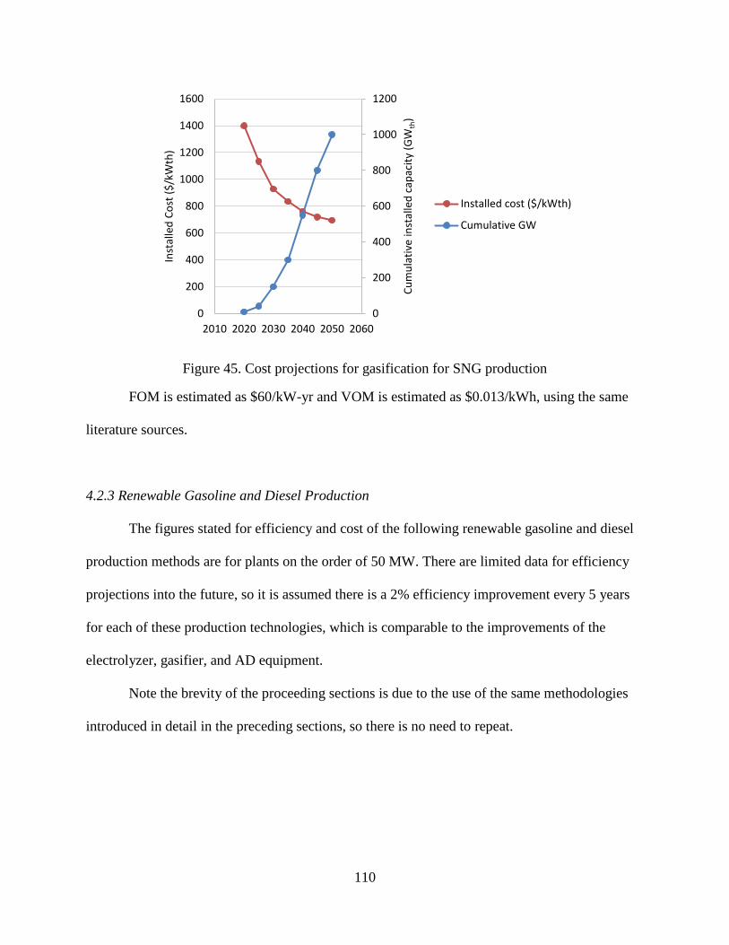
110

Figure 45. Cost projections for gasification for SNG production

FOM is estimated as $60/kW-yr and VOM is estimated as $0.013/kWh, using the same

literature sources.

4.2.3 Renewable Gasoline and Diesel Production

The figures stated for efficiency and cost of the following renewable gasoline and diesel

production methods are for plants on the order of 50 MW. There are limited data for efficiency

projections into the future, so it is assumed there is a 2% efficiency improvement every 5 years

for each of these production technologies, which is comparable to the improvements of the

electrolyzer, gasifier, and AD equipment.

Note the brevity of the proceeding sections is due to the use of the same methodologies

introduced in detail in the preceding sections, so there is no need to repeat.

0

200

400

600

800

1000

1200

0

200

400

600

800

1000

1200

1400

1600

2010 2020 2030 2040 2050 2060

Cu

mu

lati

ve in

stal

led

cap

acit

y (G

Wth

)

Inst

alle

d C

ost

($

/kW

th)

Installed cost ($/kWth)

Cumulative GW

111

4.2.3.1 Liquefaction Renewable Gasoline and Diesel Production

a) Efficiency of Liquefaction Renewable Gasoline and Diesel Production

The starting efficiency of liquefaction is modeled as 60% from Laser et al. [46], and a 2%

efficiency improvement every 5 years is assumed.

b) Cost of Liquefaction Renewable Gasoline and Diesel Production

The starting cost for liquefaction is modeled as $1440.25 per kW input from Zhu et al.

[120], and the learning rate is taken to be 10%.

4.2.3.2 Gasification and Fischer-Tropsch Renewable Gasoline and Diesel Production

a) Efficiency of Gasification and Fischer-Tropsch Renewable Gasoline and Diesel Production

The starting efficiency of gasification followed by FT is modeled as 55% from Laser et

al. [46], and a 2% efficiency improvement every 5 years is assumed.

b) Cost of Gasification and Fischer-Tropsch Renewable Gasoline and Diesel Production

The starting cost for liquefaction is modeled as $1,440.25 per kW input from Zhu et al.


4.2.3.3 Pyrolysis Renewable Gasoline and Diesel Production

a) Efficiency of Pyrolysis Renewable Gasoline and Diesel Production

The starting efficiency of pyrolysis modeled as 0.6 from Laser et al. and Jahirul et al.[46],

[242], and a 2% efficiency improvement every 5 years is assumed.

112

b) Cost of Pyrolysis Renewable Gasoline and Diesel Production

The starting cost for pyrolysis is modeled as $817.43 per kW input from Vasalos et al.


4.2.3.4 Hydrolysis Renewable Gasoline and Diesel Production

a) Efficiency of Hydrolysis Renewable Gasoline and Diesel Production

The starting efficiency of hydrolysis is modeled as 55% from Laser et al. [46], and a 2%

efficiency improvement every 5 years is assumed.

b) Cost of Hydrolysis Renewable Gasoline and Diesel Production

The starting cost for pyrolysis is modeled as $4,680 per kW input from Zhao et al.[244],

and the learning rate is taken to be 10%.

4.3 Fuel Distribution

Having detailed the techno-economics of the production of the five fuels included in the

present work, it is now the proper time to move to the distribution of each of those fuels.

4.3.1 Electricity Distribution

4.3.1.1 Efficiency of Electricity Distribution

Electricity distribution efficiency comes from losses in the electricity lines. The

efficiency modeled is 95% [245] and is held constant throughout the time of analysis.

113

4.3.1.2 Cost of Electricity Distribution

Cost of electricity distribution depends on the level of charging required. For light-duty

PHEVs and PFCEVs, which have both batteries and range extenders to power the vehicle, only

level 1 charging is needed [246][247][248]. For light-duty BEVs and all HDVs using electricity

as a fuel, some electric grid upgrades will be required to support the additional throughput.

Prior work by Lane [248] calculates the infrastructure costs for the electric grid upgrades

needed to support level 1 and level 2 charging of vehicles throughout California. Dividing those

costs by the amount of electricity the infrastructure supports as fuel for vehicles and using a CRF

of 0.12 again to annualize costs, this leads to a cost of $2.21 per GJ of electricity distributed

when using charging greater than level 1. Level 1 charging is assumed to have no distribution

cost as it uses significantly less power than an electric oven or stove [249], and therefore should

not require electric grid upgrades.

4.3.2 Hydrogen Distribution

As introduced previously, hydrogen distribution can be categorized into two segments:

from production facility to a terminal and delivery from the terminal to the dispensing station.

4.3.2.1 Efficiency of Hydrogen Distribution

The efficiency of hydrogen distribution is calculated from three components: liquefying

the hydrogen, trucking the hydrogen to the dispensing station, and any leakage that occurs during

the distribution. Liquefying is taken to be 82% energy efficient [250]. Hydrogen leakage is

assumed to be negligible as previously mentioned. Prior work shows distribution of hydrogen by

114

a hydrogen-powered HDV requires under 0.2% of the amount of hydrogen that is being

distributed [248], so the trucking portion of distribution is assumed to have negligible impact on

the efficiency of the process. Therefore, hydrogen distribution is modeled as 82% efficient

overall.

4.3.2.2 Cost of Hydrogen Distribution

Previous work shows that there is only a very slight dependency on hydrogen production

plant size for the cost of distributing hydrogen from production plant to dispensing site. The

maximum change in distribution cost was about $0.02 per kilogram of hydrogen [251]. The

range of plant considered in this work is from 21.4 MW to 500 MW. Perhaps if the range was

extended, there could be some impact of production plant scale on distribution cost, but it is

assumed in the present work that distribution cost is independent of scale of production plant.

Working with the U.S. Department of Energy’s H2A Delivery Analysis model yields

costs for the distribution and dispensing of hydrogen. Due to the way the results are displayed,

the aggregate cost of both distribution and dispensing are given here. Figure 46 shows the sum

cost of hydrogen terminals, delivery to hydrogen dispensing station, and hydrogen dispensing

station cost. The plot shows insight into factors that affect the cost of hydrogen distribution. One

is that terminal size has a significant impact on the cost of hydrogen. Increasing terminal size

decreases the cost of hydrogen. Second, the impact of terminal size diminishes as the size

continues increasing. At low terminal size (up to about 30,000 kg/day), increasing terminal size

has a dramatic decrease in cost. After about 50,000 kg/day terminal size, the effect becomes

nearly negligible.

115

Figure 46 also shows the difference in cost between gaseous hydrogen and liquid

hydrogen. At lower terminal sizes, liquid hydrogen is significantly more expensive than gaseous

hydrogen. This trend stays true for low-capacity stations no matter the terminal size. However,

mid- and high-capacity hydrogen stations, liquid hydrogen becomes cheaper than gaseous

hydrogen for larger terminal size. Recall that the present work assumes liquid hydrogen

distribution.

Figure 46. Levelized cost of hydrogen distribution and dispensing, data from [252]

A representative distribution and dispensing cost of $4.50 per kilogram of hydrogen is

used to account for variability of station cost with size.

4.3.3 SNG Distribution

SNG distribution is assumed to take the form of pipeline distribution, making use of the

prevalent pipeline infrastructure that natural gas uses today.

0

1

2

3

4

5

6

7

8

0 20,000 40,000 60,000 80,000 100,000 120,000

Leve

lized

co

st o

f h

ydro

gen

dis

trib

uti

on

an

d d

isp

ensi

ng

[$/k

g]

Terminal Size [kg/d]

GH2 - 500kg/d

GH2 - 1000kg/d

GH2 - 2000kg/d

LH2 - 500kg/d

LH2 - 1000kg/d

LH2 - 2000kg/d

116

4.3.3.1 Efficiency of SNG Distribution

SNG distribution using the natural gas pipeline is 99% efficient from a primary energy

input basis [180]. This slight efficiency loss is assumed negligible in the present work, and

therefore SNG distribution is modeled as 100% efficient.

4.3.3.2 Cost of SNG Distribution

SNG distribution costs are from Southern California Gas Company and San Diego Gas &

Electric Company, which have a customer charge of $65 each month and $0.20 per British

thermal unit (BTU) of natural gas delivered [253][254]. Even if a high estimate of 1,000 SNG

stations would be created to support HDVs in the future (a number that is one-tenth the number

of gasoline stations in California), this would yield a customer charge of $780,000 for

distribution spread among all stations. This cost is significantly less than the cost of a single

SNG station, which will be detailed shortly. Therefore, the customer charge will be neglected

and only the per-BTU charge of $0.20 will be considered in this analysis.

4.3.4 Renewable Gasoline and Diesel Distribution

Distributing renewable gasoline and diesel is assumed to be carried out in the same

manner as fossil gasoline and diesel, which is by trucking.

4.3.4.1 Efficiency of Renewable Gasoline and Diesel Distribution

Renewable liquid fuels have negligible energy losses in distribution, so they are assumed

to be 100% efficiency in the present work [180].

117

4.3.4.2 Cost of Renewable Gasoline and Diesel Distribution

According to the U.S. Energy Information Administration, approximately $0.40 to $0.60

of every gallon of gasoline and diesel sold goes to distribution and marketing [255]. It is

assumed for the present work that $0.20 of each gallon goes to distribution of the gasoline and

diesel, after removing the marketing costs included in the reference.

4.4 Fuel Dispensing

4.4.1 Electricity Dispensing

Electricity dispensing is categorized by the power output as mentioned previously. For

LDVs, PHEVs and PFCEVs use level 1 charging, and BEVs use level 2 charging

[246][247][248]. HDVs have larger battery capacities due to their lower efficiencies; therefore,

higher charging powers are needed to meet driving demands. For HDVs, the present modeling

assumes PHEVs and PFCEVs use level 2 charging and BEVs use level 3 charging.

4.4.1.1 Efficiency of Electricity Dispensing

The efficiency of electric chargers does very somewhat depending on what level the

charger is. An average value of 92% from Apostolaki-Iosifidou et al. [256] and Sears et al. [257]

is used for the present modeling .

4.4.1.2 Cost of Electricity Dispensing

Just as for efficiency, the cost of electric chargers depends on the level of charging as

well. Additionally, the amount of chargers that are to be added depend on the level of charging.

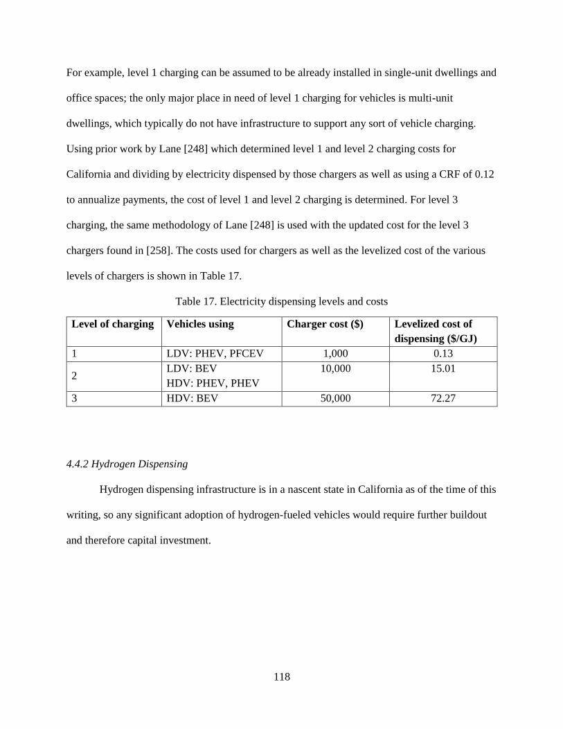
118

For example, level 1 charging can be assumed to be already installed in single-unit dwellings and

office spaces; the only major place in need of level 1 charging for vehicles is multi-unit

dwellings, which typically do not have infrastructure to support any sort of vehicle charging.

Using prior work by Lane [248] which determined level 1 and level 2 charging costs for

California and dividing by electricity dispensed by those chargers as well as using a CRF of 0.12

to annualize payments, the cost of level 1 and level 2 charging is determined. For level 3

charging, the same methodology of Lane [248] is used with the updated cost for the level 3

chargers found in [258]. The costs used for chargers as well as the levelized cost of the various

levels of chargers is shown in Table 17.

Table 17. Electricity dispensing levels and costs

Level of charging Vehicles using Charger cost ($) Levelized cost of

dispensing ($/GJ)

1 LDV: PHEV, PFCEV 1,000 0.13

2 LDV: BEV

HDV: PHEV, PHEV

10,000 15.01

3 HDV: BEV 50,000 72.27

4.4.2 Hydrogen Dispensing

Hydrogen dispensing infrastructure is in a nascent state in California as of the time of this

writing, so any significant adoption of hydrogen-fueled vehicles would require further buildout

and therefore capital investment.

119

4.4.1.1 Efficiency of Hydrogen Dispensing

Efficiencies for liquid hydrogen dispensing stations are quite high, with values ranging

from 96% from U.S. Department of Energy [252] to 97% from Hänggi et al. [180]. The average

of 96.5% efficiency is used in the present work.

4.4.1.2 Cost of Hydrogen Dispensing

A reminder here that the cost of hydrogen dispensing was incorporated with the cost of

hydrogen distribution previously. The present work is not spatially resolved, so detailed station

size for individual locations is beyond the scope of this work. Therefore, a representative

distribution and dispensing cost of $4.50 per kilogram of hydrogen are used to account for

variability of station cost with size [252].

4.4.3 SNG Dispensing

SNG is a drop-in fuel, so it can be used in existing natural gas infrastructure. However, as

previously noted in Chapter 2.1.4.3, any significant adoption of SNG-fueled HDVs would

require building out the SNG dispensing infrastructure [136][137].

4.4.1.1 Efficiency of SNG Dispensing

SNG dispensing efficiency losses are negligible according to Hänggi et al. [180], so it is

modeled as 100% efficient.

120

4.4.1.2 Cost of SNG Dispensing

Just as for hydrogen dispensing, SNG dispensing costs depend on the size of dispensing

station. For this work, assume a large station size of 1,500-2,000 GGE per day capacity, which

costs $1.8 million [259]. This large station assumption is made as the present modeling is not

spatially resolved, so a larger station size is most economical. Again using a CRF of 0.12 to

annualize payments, this. leads to $0.32 per GGE for SNG dispensing.

4.4.4 Renewable Gasoline and Diesel Dispensing

Renewable gasoline and diesel are drop-in fuels, so they can use the existing and

prevalent gasoline and diesel infrastructure.

4.4.1.1 Efficiency of Renewable Gasoline and Diesel Dispensing

Renewable liquid fuels have negligible energy losses in dispensing [180], so they are

assumed to be 100% efficiency in the present work.

4.4.1.2 Cost of Renewable Gasoline and Diesel Dispensing

Cost is negligible because gasoline and diesel stations have already been built in

abundance, so no new stations will need to be built if renewable gasoline or diesel vehicles are

projected. While in reality there is still some cost to run the stations, these costs are assumed

negligible compared to the capital of creating new stations and compared to the dispensing costs

of other fuels such as foe electric chargers or constructing SNG stations.

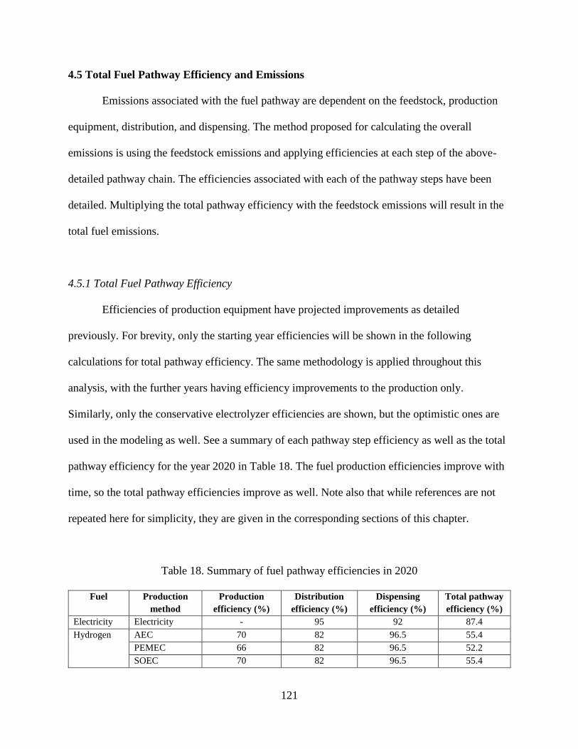
121

4.5 Total Fuel Pathway Efficiency and Emissions

Emissions associated with the fuel pathway are dependent on the feedstock, production

equipment, distribution, and dispensing. The method proposed for calculating the overall

emissions is using the feedstock emissions and applying efficiencies at each step of the above-

detailed pathway chain. The efficiencies associated with each of the pathway steps have been

detailed. Multiplying the total pathway efficiency with the feedstock emissions will result in the

total fuel emissions.

4.5.1 Total Fuel Pathway Efficiency

Efficiencies of production equipment have projected improvements as detailed

previously. For brevity, only the starting year efficiencies will be shown in the following

calculations for total pathway efficiency. The same methodology is applied throughout this

analysis, with the further years having efficiency improvements to the production only.

Similarly, only the conservative electrolyzer efficiencies are shown, but the optimistic ones are

used in the modeling as well. See a summary of each pathway step efficiency as well as the total

pathway efficiency for the year 2020 in Table 18. The fuel production efficiencies improve with

time, so the total pathway efficiencies improve as well. Note also that while references are not

repeated here for simplicity, they are given in the corresponding sections of this chapter.

Table 18. Summary of fuel pathway efficiencies in 2020

Fuel Production

method

Production

efficiency (%)

Distribution

efficiency (%)

Dispensing

efficiency (%)

Total pathway

efficiency (%)

Electricity Electricity - 95 92 87.4

Hydrogen AEC 70 82 96.5 55.4

PEMEC 66 82 96.5 52.2

SOEC 70 82 96.5 55.4

122

Gasifier 54 82 96.5 44.3

SNG AEC -

methanator

55.3 100 100 55.3

PEMEC -

methanator

52.2 100 100 52.2

SOEC -

methanator

59.3 100 100 59.3

Gasifier 67 100 100 67

AD (manure) 37 100 100 37

AD (organics) 50 100 100 50

Renewable

gasoline /

diesel

Liquefaction 64 100 100 64

Gasifier - FT 55 100 100 55

Hydrolysis 55 100 100 55

Pyrolysis 60 100 100 60

4.5.2 Feedstock Emissions

A common method of comparing the environmental impacts of various processes and

equipment is by comparing emission factors. Emission factors give the emission intensity by the

ratio of the quantity of emissions released per the amount of activity. The amount of activity can

be number of units, miles driven, or the amount of energy associated with a process. In this

work, emission factors generally take the form of quantity of emissions released per the amount

of associated energy.

Emission factors in this work are separated into two categories: (1) fuel emission factors

and (2) vehicle emission factors. Fuel emission factors consider farming, land use change by

removing the biomass to harvest for fuel, and transporting the biomass to a fuel production

facility. Note that these emissions are held constant independent of this work’s results of how

many fuel production facilities should be made and how large they should be. There is no spatial

consideration to affect the amount of biomass transportation emissions for fuel production.

Vehicle emission factors will be discussed in the following chapter.

123

Fuel emissions can be separated into two categories: electricity and biomass. In general,

the emissions associated with the fuel portion of the transportation pathway are dependent on the

feedstock (electricity or a type of biomass) and the efficiency of that pathway. While this may be

obvious for the electricity feedstock, it may not be as obvious for the biomass feedstocks. For

pathways using biomass as a feedstock, the main inputs to the fuel production processes for the

various equipment are the feedstock itself, heat, and pressure. Both heat and pressure can be

produced by simply burning some of the biomass feedstock used for fuel production. Because

the efficiencies cited in previous sections are in terms of primary energy input, this efficiency

along with the emission factor of the biomass feedstock are all that are necessary for calculating

the emissions associated with fuel production.

The present modeling assumes other emissions from the various pathway processes (for

example, the partial oxidation of pyrolysis) are negligible compared to the feedstock itself. Also

important to note is that for a given fuel production method, emissions are the same whether

producing renewable gasoline or diesel. This is due to the use of only feedstock and pathway

efficiency to calculate emissions, and efficiencies for renewable gasoline and diesel production

are modeled to be the same.

The majority of the feedstock emission factors used in this work are from Argonne

National Laboratory’s GREET 2016 [33]. More up-to-date data for electricity GHG emission

factors that account for SB 100 goals of zero-carbon electricity by 2045 are sourced from E3’s

PATHWAYS work and in particular their reference scenario [189], which projects lower GHG

emissions in later years compared to GREET; however, the CAP emission factors are sourced

from GREET as that has the most detailed CAP emissions data for electricity.

124

Due to a lack of emission factors for some biomass feedstocks, some assumptions are

made for the feedstocks that do not have data available to link them to types of biomass that they

are most similar to which do have emission factor data available. All straw biomass (barley

straw, rice hulls, rice straw, and wheat straw) are assumed to have the same emission factors as

corn stover. Residues (cotton gin trash, cotton residue, noncitrus residues, primary mill residue,

secondary mill residue, paper, paperboard, plastics, rubber, leather, textiles, yard trimmings, and

other) are all assumed to have the same emission factors as citrus residues. Both hardwood and

softwood variations are assumed to have the same emission factors as forestry. Lastly, MSW

wood is assumed to have the same emission factors as construction and demolition waste.

Two biomass categories are not present in GREET and therefore other sources were

consulted. For citrus residues (and the other biomass types that are approximated to have the

same emission factors), emission factors are sourced from Pourbafrani et al. [260]. Food waste

emission factors are taken from the California Air Resources Board [261].

Note also that GREET emissions factors are projected into 2040. For the present work,

these projections are carried out to 2050, assuming emissions factors stay the same after 2040.

For the emission factors sourced from Pourbafrani et al. [260] and the California Air Resources

Board [261], they are assumed constant throughout the timeframe of this work as there is no

indication of changing values. It should be noted that this is a valid assumption as most emission

factors are nearly constant, as will be shown shortly.

CAP emission factors for electricity are specifically for California from the “Fuel”

category of the “Electric” tab of GREET. Emission factors for the various biomass feedstocks

found in GREET are sourced from the feedstock emissions section of the various production

pathways detailed using each of the included feedstocks.

125

GHG emission factors, also known as carbon intensities (CIs), for the feedstocks are

shown in Figure 47. There are a wide range of biomass varieties with a wide range of CI values.

Note that both manure and food waste biomass feedstocks have negative CIs. This is because

both of these categories of biomass naturally release methane into the atmosphere, which has a

greater GHG impact than carbon dioxide. Turning these feedstocks into fuels stops them from

emitting methane into the atmosphere and converts most of that methane into carbon dioxide

(depending on the method of conversion). Important to note is that the CIs for electricity and

manure are on the secondary y-axis on the right side, which has a much greater magnitude of

values. The rest of the feedstocks have CIs detailed by the primary y-axis on the left side.

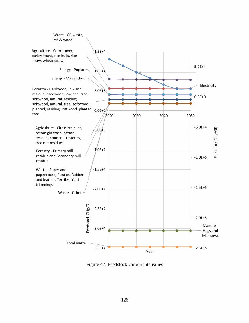
126

Figure 47. Feedstock carbon intensities

Agriculture - Corn stover, barley straw, rice hulls, rice straw, wheat straw

Agriculture - Citrus residues, cotton gin trash, cotton residue, noncitrus residues, tree nut residues

Energy - Miscanthus

Energy - Poplar

Food waste

Forestry - Hardwood, lowland, residue; hardwood, lowland, tree; softwood, natural, residue; softwood, natural, tree; softwood, planted, residue; softwood, planted, tree

Forestry - Primary mill residue and Secondary mill residue

Waste - CD waste, MSW wood

Waste - Paper and paperboard, Plastics, Rubber and leather, Textiles, Yard trimmings

Waste - Other

Electricity

Manure -Hogs and Milk cows

-2.5E+5

-2.0E+5

-1.5E+5

-1.0E+5

-5.0E+4

0.0E+0

5.0E+4

-3.5E+4

-3.0E+4

-2.5E+4

-2.0E+4

-1.5E+4

-1.0E+4

-5.0E+3

0.0E+0

5.0E+3

1.0E+4

1.5E+4

2020 2030 2040 2050

Feed

sto

ck C

I (g/

GJ)

Feed

sto

ck C

I (g/

GJ)

Year

127

The highest CI is for electricity, which is close to ten times higher than the next-highest

CI in early years of modeling. It should be noted that electricity is the only fuel feedstock with a

CI that decreases significantly with time. This is due to an increasing amount of carbon-free

renewable electricity generation being installed on the electric grid, more-efficient fossil

generation, and, perhaps most importantly, legislation such as SB 100 which require cleaner

electricity production into the future. By 2045, the CI of electricity is much more comparable to

some of the biomass feedstocks. The lowest CI is for manure, which has a very negative value.

Compared to these two extremes, all other feedstocks considered (besides food waste) have a

relatively low spread between their CIs.

Biomass feedstocks’ emission factors stay relatively constant as the emission factors

come from farming, land use change by removing the biomass to harvest for fuel, and

transporting the biomass to a fuel production facility. Both farming and land use change

emissions do not change much with time. Additionally, GREET likely assumes conventional

transport of the biomass feedstock to fuel production facilities (which will likely change). While

vehicles are assumed to be more efficient as time progresses, there is not a drastic difference in

these transportation emissions. Therefore, the overall feedstock emission factors are nearly

constant for most biomass feedstocks.

An important concept to keep in mind is that the feedstock emission factors are not the

only data that matter when determining the climate change and air quality impacts of a fuel. Also

important are the efficiency of the fuel production pathway as well as the emissions from the

vehicles themselves. Consider the following: if one feedstock has particularly low emission

factors, but it must be made using in an inefficient process and it must be used in an inefficient

vehicle, the overall emissions associated with that process may be much higher than using a

128

feedstock with higher emission factors but that can be made into a fuel more efficiently and used

in a more efficient vehicle.

However, there is a situation where the above is not true. Consider now a focus on GHG

emissions and CIs. For feedstocks with negative CIs, by definition, using more of the feedstock

to produce fuel would effectively be decreasing the climate change-inducing species in the air.

Therefore, a less-efficient fuel production process and less-efficient vehicle could be considered

better for the environment from a climate change perspective because more of the negative CI

feedstock is being used. However, consider the fact that a less-efficient process would be using

more of the feedstock. So while lower efficiency would mean a single vehicle could be helping

the environment more, this also means fewer vehicles can be fueled by that feedstock. And of

course there is only a limited amount of every feedstock available on this planet (while the

biomass feedstocks considered will replenish with time, that amount of time is not negligible).

Therefore, while negative CI feedstocks may seem to promote lower efficiency to help the

environment, that pursuit would not be a wise use of resources.

GHG and CAP emission factors for electricity are shown in Figure 48. The GHG and

CAP emission factors for the biomass feedstocks are shown in 11. APPENDIX A.

129

Figure 48. Electricity GHG and CAP emissions, data from [31], [189]

Next it is necessary to determine a representative set of emission factors for each of the

main biomass feedstock categories using the emission factors of the individual feedstocks and

the relative quantity of each feedstock. It is assumed that the relative quantities of each

individual feedstock within a category stay constant. For agriculture residue, there is a relatively

homogenous mixture of each individual feedstock, so the average is used. For energy crops,

poplar vastly outweighs miscanthus in the energy crops availability, so emission factors for

poplar are used. For food waste, there is only one feedstock. For forestry and tree, there is a

mixture of each individual feedstock, so the average is used. For manure, there is only one

feedstock. For MSW, there is a mixture of each individual feedstock, so the average is used.

0

10,000

20,000

30,000

40,000

50,000

60,000

70,000

0

5

10

15

20

25

30

35

2020 2025 2030 2035 2040 2045 2050

GH

G e

mis

sio

ns

(gC

O2

e/G

J)

CA

P e

mis

sio

ns

(g/G

J)

VOC

CO

NOx

PM10

PM2.5

SOx

BC

OC

GHGs

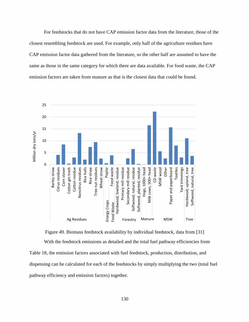
130

For feedstocks that do not have CAP emission factor data from the literature, those of the

closest resembling feedstock are used. For example, only half of the agriculture residues have

CAP emission factor data gathered from the literature, so the other half are assumed to have the

same as those in the same category for which there are data available. For food waste, the CAP

emission factors are taken from manure as that is the closest data that could be found.

Figure 49. Biomass feedstock availability by individual feedstock, data from [31]

With the feedstock emissions as detailed and the total fuel pathway efficiencies from

Table 18, the emission factors associated with fuel feedstock, production, distribution, and

dispensing can be calculated for each of the feedstocks by simply multiplying the two (total fuel

pathway efficiency and emission factors) together.

0

5

10

15

20

25

Bar

ley

stra

w

Cit

rus

resi

du

es

Co

rn s

tove

r

Co

tto

n g

in t

rash

Co

tto

n r

esid

ue

No

nci

tru

s re

sid

ues

Ric

e h

ulls

Ric

e st

raw

Tree

nu

t re

sid

ues

Wh

eat

stra

w

Po

pla

r

Foo

d w

aste

Har

dw

oo

d, l

ow

lan

d, r

esid

ue

Pri

mar

y m

ill r

esi

du

e

Seco

nd

ary

mill

res

idu

e

Soft

wo

od

, nat

ura

l, re

sid

ue

Soft

wo

od

, pla

nte

d, r

esid

ue

Ho

gs, 1

00

0+

he

ad

Milk

co

ws,

50

0+

he

ad

CD

was

te

MSW

wo

od

Oth

er

Pap

er a

nd

pap

erb

oar

d

Text

iles

Yard

tri

mm

ings

Har

dw

oo

d, u

pla

nd

, tre

e

Soft

wo

od

, nat

ura

l, tr

ee

Ag Residues EnergyFood WasteForest ResiduesManure MSW Tree

Mill

ion

dry

to

ns/

yr

Ener

gy C

rop

s

Foo

d W

aste

Forestry

Energy Crops

Manure

Energy Crops

131

5. VEHICLE POWERTRAIN CONFIGURATIONS

Both LDVs and HDVs are modeled in this work, and their powertrain configuration

options are largely the same (except for the fact that LDVs with combustion engines are fueled

by gasoline while HDVs with combustion engines are fueled by either diesel or SNG). Four main

HDV class 8 categories are used in this work: long-haul, drayage, refuse, and construction. These

categories were selected based on the number of miles traveled and the amount of GHG and

CAP emissions from them. Four were selected to have a balance between adequately

representing the wide range of HDVs (each with their own powertrain specifications) without

going beyond the scope of this work and getting lost in the vast amount of work that must be

done to characterize every single HDV category.

As for the fuel production work, again a 2% rate of inflation is assumed [187] and a CRF

of 0.12 is used to annualize costs of vehicles [188].

5.1 Vehicle Efficiencies

Efficiencies for the various powertrain configurations for LDVs are taken from current

popular vehicles in their respective categories. The ICV is represented by the Toyota Corolla, the

HEV by the Toyota Prius, the PHEV by the Toyota Prius Prime, the BEV by the Chevrolet Bolt,

and the FCEV by the Toyota Mirai. One exception to this methodology is the PFCEV, which

currently does not have a publically available option. Instead the literature is consulted, and the

efficiency data are taken from Lane et al. [26].

Shown in Table 19 are the efficiencies of each of the LDV powertrains mentioned above

for the simulation year 2020, and Table 20 shows the same for HDVs. Efficiency projections into

the future will be detailed shortly. The “vehicle efficiency” number is the typical miles per gallon

132

(MPG) or miles per gallon of gasoline equivalent (MPGGE) that one typically sees for LDVs.

For vehicles that have both battery and a range extender, this efficiency is known as the charge

sustaining (CS) efficiency as it is the efficiency of the vehicle when not using the battery. The

“charge depleting (CD) efficiency” is applicable only for PEVs, and it is the efficiency of the

vehicle when driven on the battery alone, depleting its charge. In comparison, for PEVs, the

former “vehicle efficiency” could be considered the charge sustaining (CS) efficiency, meaning

the electric charge of the vehicle is held constant and only the range extender is used, if one is

available. The CD efficiency is shown in kilowatt-hours per mile. Note that the BEV efficiency

is not shown as the CD efficiency as the battery is the only source of power for BEVs and

efficiency is easier to compare using the MPGGE value. The sources of data are given in the

table.

Table 20 shows the HDV efficiencies for the year 2020. The efficiencies are shown in

miles per gallon of diesel equivalent (MPGDE) to make comparisons with conventional HDVs

easier. The CD efficiency is again shown in kilowatt-hours per mile. Determining these

efficiencies for HDVs is more involved than for LDVs because not all of the powertrains are

available purchase or have much public information at the time of this work.

First is a focus on linehaul HDVs. The efficiencies for the ICV, HEV, PHEV, BEV, and

FCEV linehaul vehicles are from Zhao et al. [262]. The CS efficiency for the HDV PHEV is

determined by taking the ratio of the LDV PHEV CS efficiency compared to the LDV HEV

efficiency and multiplying that ratio to the efficiency of the corresponding HDV HEV. The

methodology is captured in Equation 8.

Equation 8. CS efficiency of HDV PHEV

𝜂𝐶𝑆,𝐻𝐷𝑉 𝑃𝐻𝐸𝑉 =𝜂𝐶𝑆,𝐿𝐷𝑉 𝑃𝐻𝐸𝑉𝜂𝐿𝐷𝑉 𝐻𝐸𝑉

∗ 𝜂𝐻𝐷𝑉 𝐻𝐸𝑉

133

The CD efficiency of the HDV PHEV is obtained by multiplying the above CS efficiency for the

vehicle by the ratio of CD efficiency to CS efficiency of the LDV PHEV. The methodology is

captured in Equation 9.

Equation 9. CD efficiency of HDV PHEV

𝜂𝐶𝐷,𝐻𝐷𝑉 𝑃𝐻𝐸𝑉 =𝜂𝐶𝐷,𝐿𝐷𝑉 𝑃𝐻𝐸𝑉𝜂𝐶𝑆,𝐿𝐷𝑉 𝑃𝐻𝐸𝑉

∗ 𝜂𝐶𝑆,𝐻𝐷𝑉 𝑃𝐻𝐸𝑉

The CS efficiency for the PFCEV is determined by taking the ratio of LDV PFCEV compared to

the FCEV and multiplying that ratio by the efficiency of the HDV FCEV, as shown in Equation

10.

Equation 10. CS efficiency of HDV PFCEV

𝜂𝐶𝑆,𝐻𝐷𝑉 𝑃𝐹𝐶𝐸𝑉 =𝜂𝐶𝑆,𝐿𝐷𝑉 𝑃𝐹𝐶𝐸𝑉𝜂𝐿𝐷𝑉 𝐹𝐶𝐸𝑉

∗ 𝜂𝐻𝐷𝑉 𝐹𝐶𝐸𝑉

The CD efficiency of the HDV PFCEV is obtained by multiplying the above efficiency by the

ratio of the CD efficiency of the LDV PFCEV to the efficiency of the LDV PFCEV, as shown in

Equation 11.

Equation 11. CD efficiency of HDV PFCEV

𝜂𝐶𝐷,𝐻𝐷𝑉 𝑃𝐹𝐶𝐸𝑉 =𝜂𝐶𝐷,𝐿𝐷𝑉 𝑃𝐹𝐶𝐸𝑉𝜂𝐶𝑆,𝐿𝐷𝑉 𝑃𝐹𝐶𝐸𝑉

∗ 𝜂𝐶𝑆,𝐻𝐷𝑉 𝑃𝐹𝐶𝐸𝑉

The sources for all of the LDV efficiencies used in these processes are given in Table 19.

Next is to determine the efficiencies of the other vocations for the HDVs. Work by Kast et al.

[263] is used to extrapolate the linehaul efficiencies to the three other HDV vocations of the

present work. Kast et al. details the differences in efficiency for FCEVs by vocation using an

appropriate duty cycle for the simulation of the vehicles. While the work only details the

efficiencies for FCEVs, the present work assumes those efficiency differences will carry across

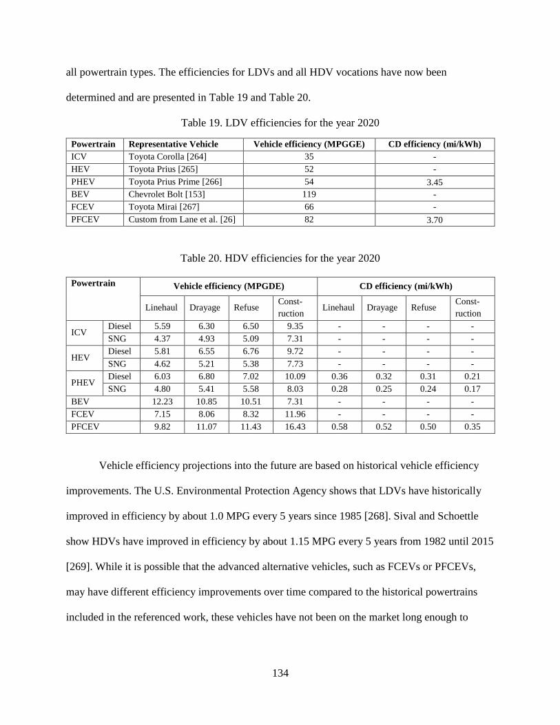
134

all powertrain types. The efficiencies for LDVs and all HDV vocations have now been

determined and are presented in Table 19 and Table 20.

Table 19. LDV efficiencies for the year 2020

Powertrain Representative Vehicle Vehicle efficiency (MPGGE) CD efficiency (mi/kWh)

ICV Toyota Corolla [264] 35 -

HEV Toyota Prius [265] 52 -

PHEV Toyota Prius Prime [266] 54 3.45

BEV Chevrolet Bolt [153] 119 -

FCEV Toyota Mirai [267] 66 -

PFCEV Custom from Lane et al. [26] 82 3.70

Table 20. HDV efficiencies for the year 2020

Powertrain Vehicle efficiency (MPGDE) CD efficiency (mi/kWh)

Linehaul Drayage Refuse Const-

ruction Linehaul Drayage Refuse

Const-

ruction

ICV Diesel 5.59 6.30 6.50 9.35 - - - -

SNG 4.37 4.93 5.09 7.31 - - - -

HEV Diesel 5.81 6.55 6.76 9.72 - - - -

SNG 4.62 5.21 5.38 7.73 - - - -

PHEV Diesel 6.03 6.80 7.02 10.09 0.36 0.32 0.31 0.21

SNG 4.80 5.41 5.58 8.03 0.28 0.25 0.24 0.17

BEV 12.23 10.85 10.51 7.31 - - - -

FCEV 7.15 8.06 8.32 11.96 - - - -

PFCEV 9.82 11.07 11.43 16.43 0.58 0.52 0.50 0.35

Vehicle efficiency projections into the future are based on historical vehicle efficiency

improvements. The U.S. Environmental Protection Agency shows that LDVs have historically

improved in efficiency by about 1.0 MPG every 5 years since 1985 [268]. Sival and Schoettle

show HDVs have improved in efficiency by about 1.15 MPG every 5 years from 1982 until 2015

[269]. While it is possible that the advanced alternative vehicles, such as FCEVs or PFCEVs,

may have different efficiency improvements over time compared to the historical powertrains

included in the referenced work, these vehicles have not been on the market long enough to

135

determine if there will be any significant difference in efficiency evolution. Therefore, the

assumption of using the same projection is used due to the lack of more-detailed information.

5.2 Vehicle Costs

The approach for determining vehicle costs is two-fold. First, similar to the methodology

of the LDV efficiency, LDV cost is also gathered from popular vehicles currently available for

purchase. The manufacturer’s suggested retail price (MSRP) is used as proxy for the cost. Again,

the PFCEV is an exception due to its lack of current availability. For the PFCEV cost, a ratio of

PHEV to HEV cost was multiplied to the cost of the FCEV, which is itself a hybrid. This

approximation attempts to determine costs that are not yet well-understood, at least outside of a

vehicle manufacturer, but this method should account for the difference in cost of the PFCEV

compared to the FCEV due to a larger battery, smaller fuel cell, and the accompanying

electronics upgrades. The values from this approach are not used in the present modeling, but are

instead used to gauge the results of the following method to ensure reasonable starting values.

The second approach is to categorize vehicle cost by components, categorizing vehicles

into powertrain components such as internal combustion engine (ICE), battery, etc., and

everything else which is known as the vehicle glider, such as the chassis and wheels. The reason

for this is that each vehicle component will have different learning rates (LRs) associated with

them. For example, the vehicle glider which is a very mature technology, will have a lower LR

compared to a fuel cell, which is a much less mature technology. Note that the default LRs used

are reminiscent of those for some of the fuel production technologies. A LR of 0.1 is used for

more mature technologies, and a LR of 0.14 is used for less mature technologies. Both the costs

and LRs for each of the major vehicle components is listed in Table 21. Note the hybrid and

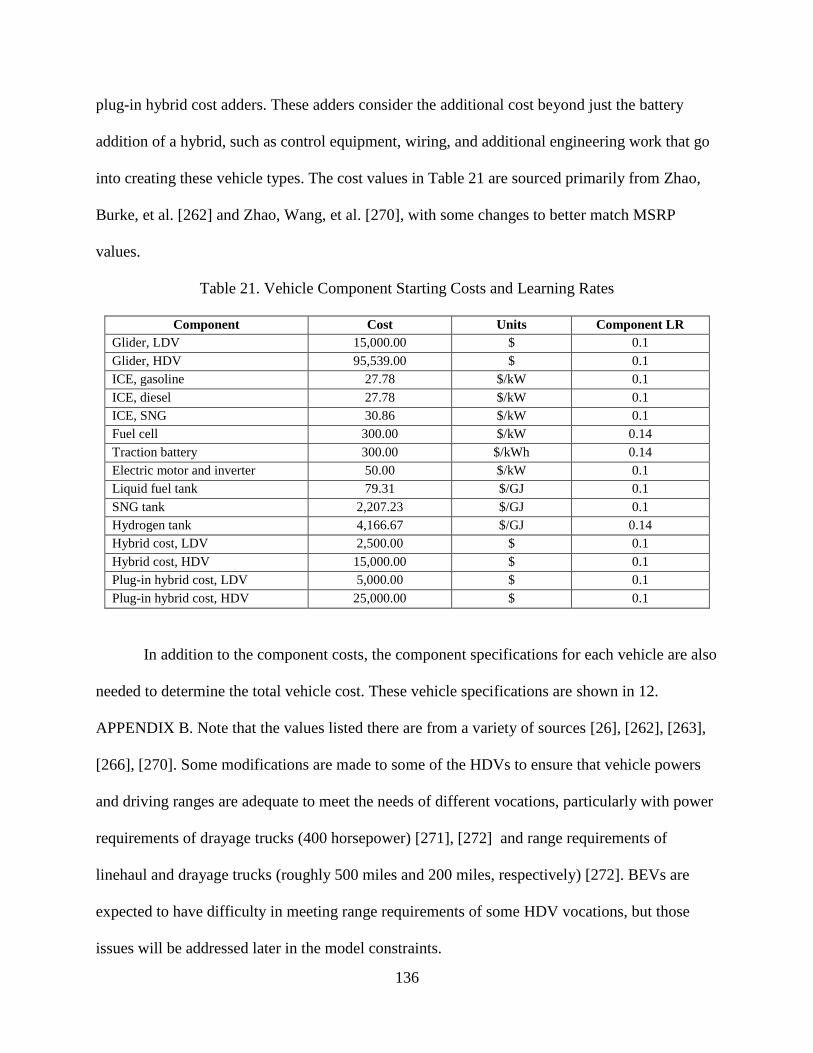
136

plug-in hybrid cost adders. These adders consider the additional cost beyond just the battery

addition of a hybrid, such as control equipment, wiring, and additional engineering work that go

into creating these vehicle types. The cost values in Table 21 are sourced primarily from Zhao,

Burke, et al. [262] and Zhao, Wang, et al. [270], with some changes to better match MSRP

values.

Table 21. Vehicle Component Starting Costs and Learning Rates

Component Cost Units Component LR

Glider, LDV 15,000.00 $ 0.1

Glider, HDV 95,539.00 $ 0.1

ICE, gasoline 27.78 $/kW 0.1

ICE, diesel 27.78 $/kW 0.1

ICE, SNG 30.86 $/kW 0.1

Fuel cell 300.00 $/kW 0.14

Traction battery 300.00 $/kWh 0.14

Electric motor and inverter 50.00 $/kW 0.1

Liquid fuel tank 79.31 $/GJ 0.1

SNG tank 2,207.23 $/GJ 0.1

Hydrogen tank 4,166.67 $/GJ 0.14

Hybrid cost, LDV 2,500.00 $ 0.1

Hybrid cost, HDV 15,000.00 $ 0.1

Plug-in hybrid cost, LDV 5,000.00 $ 0.1

Plug-in hybrid cost, HDV 25,000.00 $ 0.1

In addition to the component costs, the component specifications for each vehicle are also

needed to determine the total vehicle cost. These vehicle specifications are shown in 12.

APPENDIX B. Note that the values listed there are from a variety of sources [26], [262], [263],

[266], [270]. Some modifications are made to some of the HDVs to ensure that vehicle powers

and driving ranges are adequate to meet the needs of different vocations, particularly with power

requirements of drayage trucks (400 horsepower) [271], [272] and range requirements of

linehaul and drayage trucks (roughly 500 miles and 200 miles, respectively) [272]. BEVs are

expected to have difficulty in meeting range requirements of some HDV vocations, but those

issues will be addressed later in the model constraints.

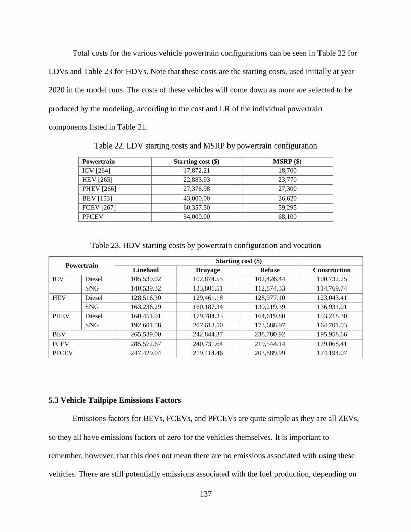
137

Total costs for the various vehicle powertrain configurations can be seen in Table 22 for

LDVs and Table 23 for HDVs. Note that these costs are the starting costs, used initially at year

2020 in the model runs. The costs of these vehicles will come down as more are selected to be

produced by the modeling, according to the cost and LR of the individual powertrain

components listed in Table 21.

Table 22. LDV starting costs and MSRP by powertrain configuration

Powertrain Starting cost ($) MSRP ($)

ICV [264] 17,872.21 18,700

HEV [265] 22,883.93 23,770

PHEV [266] 27,376.98 27,300

BEV [153] 43,000.00 36,620

FCEV [267] 60,357.50 59,295

PFCEV 54,000.00 68,100

Table 23. HDV starting costs by powertrain configuration and vocation

Powertrain Starting cost ($)

Linehaul Drayage Refuse Construction

ICV Diesel 105,539.02 102,874.55 102,426.44 100,732.75

SNG 140,539.32 133,801.51 112,874.33 114,769.74

HEV Diesel 128,516.30 129,461.18 128,977.10 123,043.41

SNG 163,236.29 160,187.34 139,219.39 136,931.01

PHEV Diesel 160,451.91 179,784.33 164,619.80 153,218.30

SNG 192,601.58 207,613.50 173,688.97 164,701.03

BEV 265,539.00 242,844.37 238,780.92 195,958.66

FCEV 285,572.67 240,731.64 219,544.14 179,068.41

PFCEV 247,429.04 219,414.46 203,889.99 174,194.07

5.3 Vehicle Tailpipe Emissions Factors

Emissions factors for BEVs, FCEVs, and PFCEVs are quite simple as they are all ZEVs,

so they all have emissions factors of zero for the vehicles themselves. It is important to

remember, however, that this does not mean there are no emissions associated with using these

vehicles. There are still potentially emissions associated with the fuel production, depending on

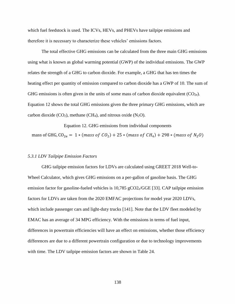
138

which fuel feedstock is used. The ICVs, HEVs, and PHEVs have tailpipe emissions and

therefore it is necessary to characterize these vehicles’ emissions factors.

The total effective GHG emissions can be calculated from the three main GHG emissions

using what is known as global warming potential (GWP) of the individual emissions. The GWP

relates the strength of a GHG to carbon dioxide. For example, a GHG that has ten times the

heating effect per quantity of emission compared to carbon dioxide has a GWP of 10. The sum of

GHG emissions is often given in the units of some mass of carbon dioxide equivalent (CO2e).

Equation 12 shows the total GHG emissions given the three primary GHG emissions, which are

carbon dioxide (CO2), methane (CH4), and nitrous oxide (N2O).

Equation 12. GHG emissions from individual components

mass of GHG, CO2e = 1 ∗ (𝑚𝑎𝑠𝑠 𝑜𝑓 𝐶𝑂2) + 25 ∗ (𝑚𝑎𝑠𝑠 𝑜𝑓 𝐶𝐻4) + 298 ∗ (𝑚𝑎𝑠𝑠 𝑜𝑓 𝑁2𝑂)

5.3.1 LDV Tailpipe Emission Factors

GHG tailpipe emission factors for LDVs are calculated using GREET 2018 Well-to-

Wheel Calculator, which gives GHG emissions on a per-gallon of gasoline basis. The GHG

emission factor for gasoline-fueled vehicles is 10,785 gCO2e/GGE [33]. CAP tailpipe emission

factors for LDVs are taken from the 2020 EMFAC projections for model year 2020 LDVs,

which include passenger cars and light-duty trucks [141]. Note that the LDV fleet modeled by

EMAC has an average of 34 MPG efficiency. With the emissions in terms of fuel input,

differences in powertrain efficiencies will have an effect on emissions, whether those efficiency

differences are due to a different powertrain configuration or due to technology improvements

with time. The LDV tailpipe emission factors are shown in Table 24.

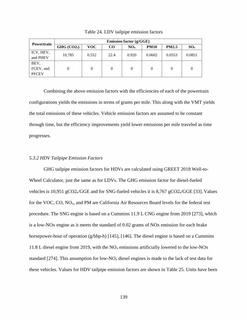
139

Table 24. LDV tailpipe emission factors

Powertrain Emission factor (g/GGE)

GHG (CO2e) VOC CO NOx PM10 PM2.5 SOx

ICV, HEV,

and PHEV 10,785 0.552 22.4 0.920 0.0602 0.0553 0.0851

BEV,

FCEV, and

PFCEV

0 0 0 0 0 0 0

Combining the above emission factors with the efficiencies of each of the powertrain

configurations yields the emissions in terms of grams per mile. This along with the VMT yields

the total emissions of these vehicles. Vehicle emission factors are assumed to be constant

through time, but the efficiency improvements yield lower emissions per mile traveled as time

progresses.

5.3.2 HDV Tailpipe Emission Factors

GHG tailpipe emission factors for HDVs are calculated using GREET 2018 Well-to-

Wheel Calculator, just the same as for LDVs. The GHG emission factor for diesel-fueled

vehicles is 10,951 gCO2e/GGE and for SNG-fueled vehicles it is 8,767 gCO2e/GGE [33]. Values

for the VOC, CO, NOx, and PM are California Air Resources Board levels for the federal test

procedure. The SNG engine is based on a Cummins 11.9 L CNG engine from 2019 [273], which

is a low-NOx engine as it meets the standard of 0.02 grams of NOx emission for each brake

horsepower-hour of operation (g/bhp-h) [145], [146]. The diesel engine is based on a Cummins

11.8 L diesel engine from 2019, with the NOx emissions artificially lowered to the low-NOx

standard [274]. This assumption for low-NOx diesel engines is made to the lack of test data for

these vehicles. Values for HDV tailpipe emission factors are shown in Table 25. Units have been

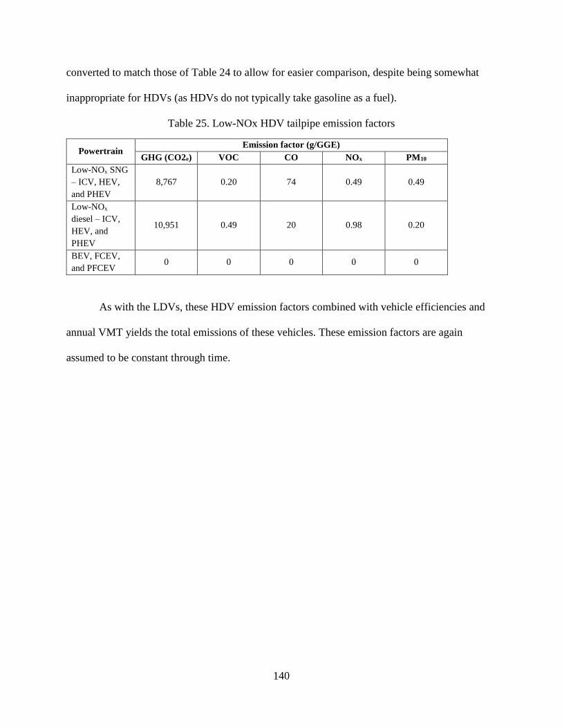
140

converted to match those of Table 24 to allow for easier comparison, despite being somewhat

inappropriate for HDVs (as HDVs do not typically take gasoline as a fuel).

Table 25. Low-NOx HDV tailpipe emission factors

Powertrain Emission factor (g/GGE)

GHG (CO2e) VOC CO NOx PM10

Low-NOx SNG

– ICV, HEV,

and PHEV

8,767 0.20 74 0.49 0.49

Low-NOx

diesel – ICV,

HEV, and

PHEV

10,951 0.49 20 0.98 0.20

BEV, FCEV,

and PFCEV 0 0 0 0 0

As with the LDVs, these HDV emission factors combined with vehicle efficiencies and

annual VMT yields the total emissions of these vehicles. These emission factors are again

assumed to be constant through time.

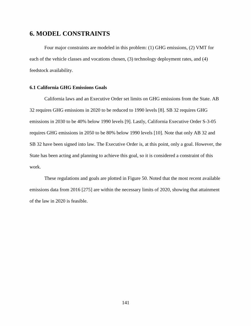
141

6. MODEL CONSTRAINTS

Four major constraints are modeled in this problem: (1) GHG emissions, (2) VMT for

each of the vehicle classes and vocations chosen, (3) technology deployment rates, and (4)

feedstock availability.

6.1 California GHG Emissions Goals

California laws and an Executive Order set limits on GHG emissions from the State. AB

32 requires GHG emissions in 2020 to be reduced to 1990 levels [8]. SB 32 requires GHG

emissions in 2030 to be 40% below 1990 levels [9]. Lastly, California Executive Order S-3-05

requires GHG emissions in 2050 to be 80% below 1990 levels [10]. Note that only AB 32 and

SB 32 have been signed into law. The Executive Order is, at this point, only a goal. However, the

State has been acting and planning to achieve this goal, so it is considered a constraint of this

work.

These regulations and goals are plotted in Figure 50. Noted that the most recent available

emissions data from 2016 [275] are within the necessary limits of 2020, showing that attainment

of the law in 2020 is feasible.

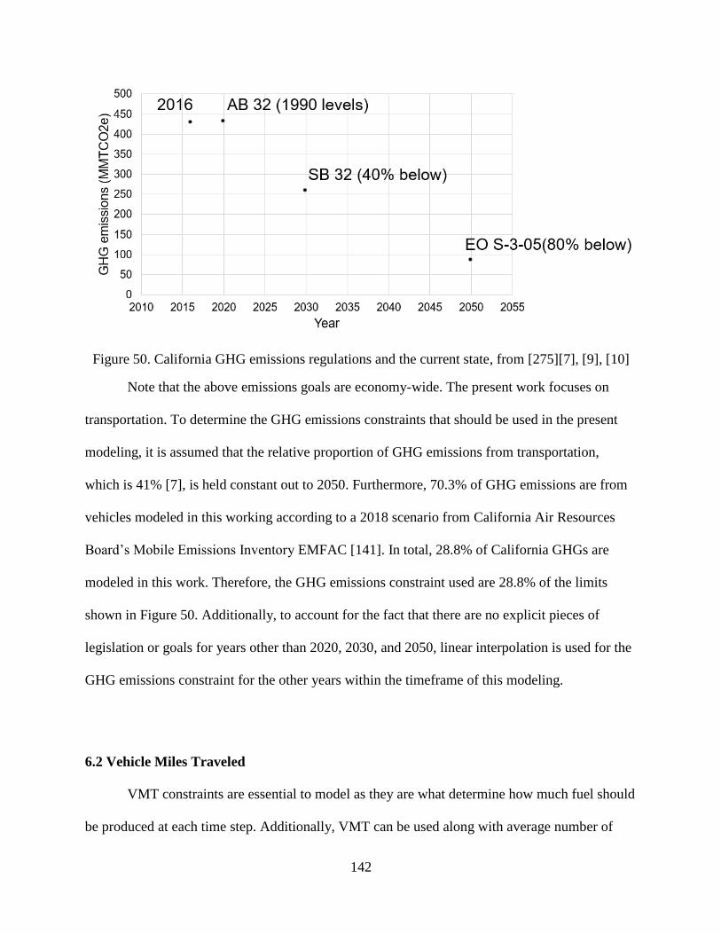
142

Figure 50. California GHG emissions regulations and the current state, from [275][7], [9], [10]

Note that the above emissions goals are economy-wide. The present work focuses on

transportation. To determine the GHG emissions constraints that should be used in the present

modeling, it is assumed that the relative proportion of GHG emissions from transportation,

which is 41% [7], is held constant out to 2050. Furthermore, 70.3% of GHG emissions are from

vehicles modeled in this working according to a 2018 scenario from California Air Resources

Board’s Mobile Emissions Inventory EMFAC [141]. In total, 28.8% of California GHGs are

modeled in this work. Therefore, the GHG emissions constraint used are 28.8% of the limits

shown in Figure 50. Additionally, to account for the fact that there are no explicit pieces of

legislation or goals for years other than 2020, 2030, and 2050, linear interpolation is used for the

GHG emissions constraint for the other years within the timeframe of this modeling.

6.2 Vehicle Miles Traveled

VMT constraints are essential to model as they are what determine how much fuel should

be produced at each time step. Additionally, VMT can be used along with average number of

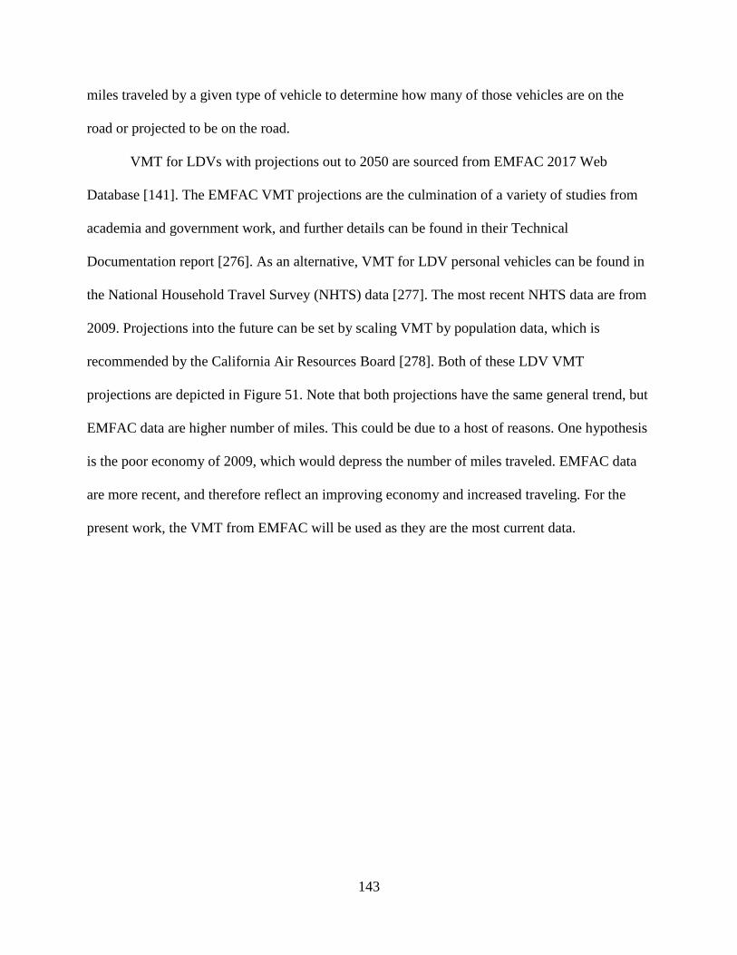
143

miles traveled by a given type of vehicle to determine how many of those vehicles are on the

road or projected to be on the road.

VMT for LDVs with projections out to 2050 are sourced from EMFAC 2017 Web

Database [141]. The EMFAC VMT projections are the culmination of a variety of studies from

academia and government work, and further details can be found in their Technical

Documentation report [276]. As an alternative, VMT for LDV personal vehicles can be found in

the National Household Travel Survey (NHTS) data [277]. The most recent NHTS data are from

2009. Projections into the future can be set by scaling VMT by population data, which is

recommended by the California Air Resources Board [278]. Both of these LDV VMT

projections are depicted in Figure 51. Note that both projections have the same general trend, but

EMFAC data are higher number of miles. This could be due to a host of reasons. One hypothesis

is the poor economy of 2009, which would depress the number of miles traveled. EMFAC data

are more recent, and therefore reflect an improving economy and increased traveling. For the

present work, the VMT from EMFAC will be used as they are the most current data.

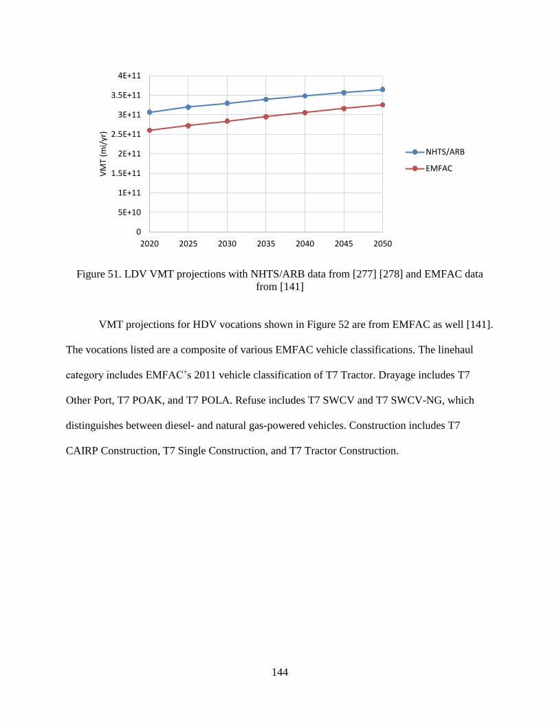
144

Figure 51. LDV VMT projections with NHTS/ARB data from [277] [278] and EMFAC data

from [141]

VMT projections for HDV vocations shown in Figure 52 are from EMFAC as well [141].

The vocations listed are a composite of various EMFAC vehicle classifications. The linehaul

category includes EMFAC’s 2011 vehicle classification of T7 Tractor. Drayage includes T7

Other Port, T7 POAK, and T7 POLA. Refuse includes T7 SWCV and T7 SWCV-NG, which

distinguishes between diesel- and natural gas-powered vehicles. Construction includes T7

CAIRP Construction, T7 Single Construction, and T7 Tractor Construction.

0

5E+10

1E+11

1.5E+11

2E+11

2.5E+11

3E+11

3.5E+11

4E+11

2020 2025 2030 2035 2040 2045 2050

VM

T (m

i/yr

)

NHTS/ARB

EMFAC

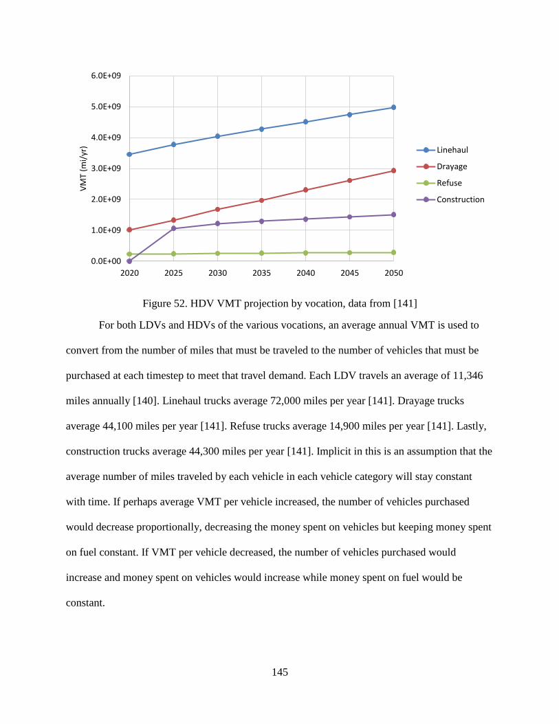
145

Figure 52. HDV VMT projection by vocation, data from [141]

For both LDVs and HDVs of the various vocations, an average annual VMT is used to

convert from the number of miles that must be traveled to the number of vehicles that must be

purchased at each timestep to meet that travel demand. Each LDV travels an average of 11,346

miles annually [140]. Linehaul trucks average 72,000 miles per year [141]. Drayage trucks

average 44,100 miles per year [141]. Refuse trucks average 14,900 miles per year [141]. Lastly,

construction trucks average 44,300 miles per year [141]. Implicit in this is an assumption that the

average number of miles traveled by each vehicle in each vehicle category will stay constant

with time. If perhaps average VMT per vehicle increased, the number of vehicles purchased

would decrease proportionally, decreasing the money spent on vehicles but keeping money spent

on fuel constant. If VMT per vehicle decreased, the number of vehicles purchased would

increase and money spent on vehicles would increase while money spent on fuel would be

constant.

0.0E+00

1.0E+09

2.0E+09

3.0E+09

4.0E+09

5.0E+09

6.0E+09

2020 2025 2030 2035 2040 2045 2050

VM

T (m

i/yr

) Linehaul

Drayage

Refuse

Construction

146

One additional constraint concerning the VMT constraints is the BEV’s relatively low

driving range and long fueling time compared to other vehicle powertrain configurations.

The BEV modeled for LDVs has a range of 200 miles given its efficiency and traction

battery size. This range is similar to that of modern-day BEVs like the Tesla Model 3 and the

Chevrolet Bolt, among many others that are coming onto the market. While this range is

significantly higher than that of BEVs from years past, it is noticeably less than ICVs and all

other alternative powertrain configurations with ranges above 300 miles. As previously noted in

Chapter 2.2.4, BEVs also have charging times much longer than drivers are accustomed to at

gasoline stations. Karlsson notes that 79% of households with a BEV have more than one car,

compared to 48% for those with conventional vehicles [279]. One may hypothesize that this is

simply due to the fact that BEVs owners are simply more wealthy and have more vehicles. This

is not so. The 79% figure increases when removing the Tesla Model S, an expensive and longer-

range BEV. Therefore, the proclivity of BEV owners having multiple cars is significantly related

to the short driving range and long fueling times of BEVs.

With 21% of BEV owners having only one vehicle, and the rest having at least two

vehicles (meaning at most half of the remaining 79% of vehicles are BEVs), this means at most a

total of 61% of LDVs could conceivably be BEVs, due to driving range and fueling time

limitations. Assuming this 61% of vehicles translates to 61% of VMT, the light-duty VMT is

herein modeled to be composed of at most 61% BEV VMT.

As previously mentioned for HDVs, as of 2015, only drayage and refuse trucks had been

demonstrated to operate with a BEV powertrain due to range limitations [157]. Some literature

predict low class 8 BEV feasibility of up to about 20% unless higher charging rates or battery

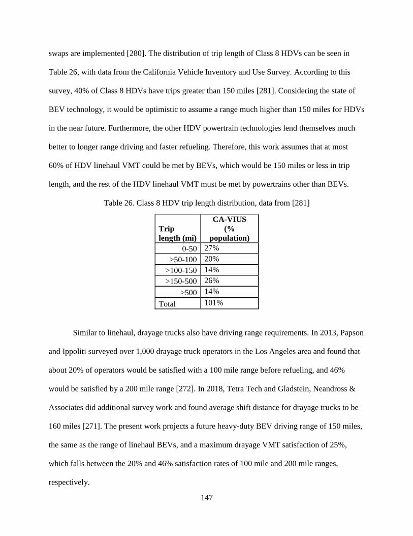
147

swaps are implemented [280]. The distribution of trip length of Class 8 HDVs can be seen in

Table 26, with data from the California Vehicle Inventory and Use Survey. According to this

survey, 40% of Class 8 HDVs have trips greater than 150 miles [281]. Considering the state of

BEV technology, it would be optimistic to assume a range much higher than 150 miles for HDVs

in the near future. Furthermore, the other HDV powertrain technologies lend themselves much

better to longer range driving and faster refueling. Therefore, this work assumes that at most

60% of HDV linehaul VMT could be met by BEVs, which would be 150 miles or less in trip

length, and the rest of the HDV linehaul VMT must be met by powertrains other than BEVs.

Table 26. Class 8 HDV trip length distribution, data from [281]

Trip

length (mi)

CA-VIUS

(%

population)

0-50 27%

>50-100 20%

>100-150 14%

>150-500 26%

>500 14%

Total 101%

Similar to linehaul, drayage trucks also have driving range requirements. In 2013, Papson

and Ippoliti surveyed over 1,000 drayage truck operators in the Los Angeles area and found that

about 20% of operators would be satisfied with a 100 mile range before refueling, and 46%

would be satisfied by a 200 mile range [272]. In 2018, Tetra Tech and Gladstein, Neandross &

Associates did additional survey work and found average shift distance for drayage trucks to be

160 miles [271]. The present work projects a future heavy-duty BEV driving range of 150 miles,

the same as the range of linehaul BEVs, and a maximum drayage VMT satisfaction of 25%,

which falls between the 20% and 46% satisfaction rates of 100 mile and 200 mile ranges,

respectively.

148

The refuse and construction HDV vocations are assumed able to be met fully by BEVs as

their trip lengths are not as high as linehaul or drayage.

6.2.1 Utility Factor

The utility factor (UF) of a vehicle specifies how many of the miles that vehicle travels

using the battery as the power source compared to the total number of miles traveled. An ICV

has a UF of 0 because it has no battery to supply driving power, a BEV has a UF of 1 because it

has only a battery to supply driving power, and a PHEV or PFCEV can have a UF anywhere

from 0 to 1, depending on how the vehicle is driven and fueled. For example, a PFCEV that

travels 30 miles on its battery charge and 70 miles using hydrogen in the fuel cell has a UF of 0.3

for that trip. UFs vary greatly by vehicle specification (BER, CD efficiency, CS efficiency), trip

composition (length, grade, etc.), fueling habits (whether one charges the vehicle at home or

not), driving personalities (speed, acceleration, etc.), and other factors. Therefore, it is most

practical to use an average UF that represents the spectrum of possibilities.

The Society of Automotive Engineers (SAE) International defines a particular UF as a

fleet UF (FUF). SAE International suggests using the FUF to determine the electricity and other

fuel use for a fleet of vehicles, which is the intended use in the present work. The FUF is

calculated using a distribution of vehicle trips and dividing the miles of CD travel by the total

number of trip miles [282].

Using the SAE International J2841 specification along with BER specifications with a

vehicle yields the FUF. The FUF for LDVs and each vocation of HDVs are shown in Table 27,

using the BER and FUF correlation from SAE International J2841 [282]. LDVs for this work are

designed with a BER of approximately 40 miles [26][283][284]. The BER for the various HDV

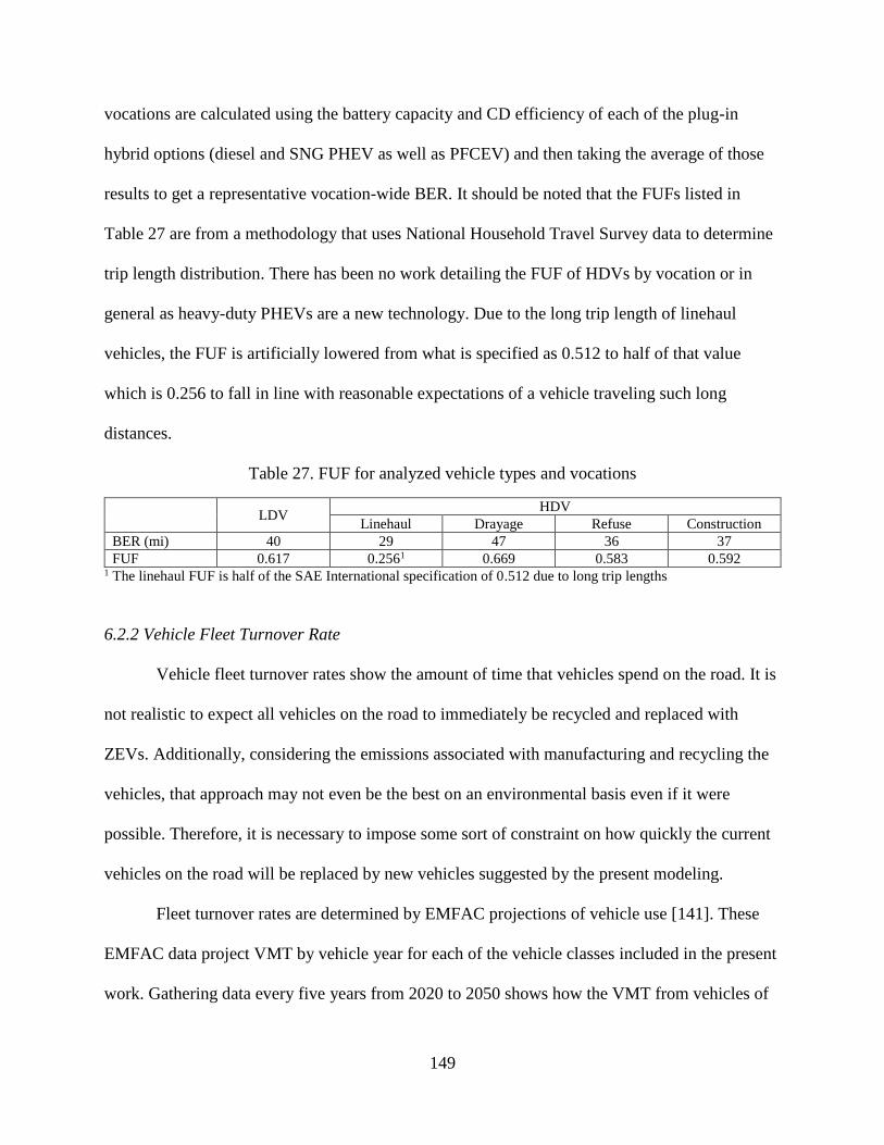
149

vocations are calculated using the battery capacity and CD efficiency of each of the plug-in

hybrid options (diesel and SNG PHEV as well as PFCEV) and then taking the average of those

results to get a representative vocation-wide BER. It should be noted that the FUFs listed in

Table 27 are from a methodology that uses National Household Travel Survey data to determine

trip length distribution. There has been no work detailing the FUF of HDVs by vocation or in

general as heavy-duty PHEVs are a new technology. Due to the long trip length of linehaul

vehicles, the FUF is artificially lowered from what is specified as 0.512 to half of that value

which is 0.256 to fall in line with reasonable expectations of a vehicle traveling such long

distances.

Table 27. FUF for analyzed vehicle types and vocations

LDV

HDV

Linehaul Drayage Refuse Construction

BER (mi) 40 29 47 36 37

FUF 0.617 0.2561 0.669 0.583 0.592 1 The linehaul FUF is half of the SAE International specification of 0.512 due to long trip lengths

6.2.2 Vehicle Fleet Turnover Rate

Vehicle fleet turnover rates show the amount of time that vehicles spend on the road. It is

not realistic to expect all vehicles on the road to immediately be recycled and replaced with

ZEVs. Additionally, considering the emissions associated with manufacturing and recycling the

vehicles, that approach may not even be the best on an environmental basis even if it were

possible. Therefore, it is necessary to impose some sort of constraint on how quickly the current

vehicles on the road will be replaced by new vehicles suggested by the present modeling.

Fleet turnover rates are determined by EMFAC projections of vehicle use [141]. These

EMFAC data project VMT by vehicle year for each of the vehicle classes included in the present

work. Gathering data every five years from 2020 to 2050 shows how the VMT from vehicles of

150

prior years decreases as time goes on. Germane to the present work are the VMT from vehicles

made prior to 2020, as vehicles made in 2020 and beyond to 2050 will be dictated by the

optimization.

Also available in this data set from EMFAC are emissions from the vehicles from

different years. Again, emissions from vehicles made prior to 2020 are gathered, and taken to be

baseline emissions that will occur regardless of what the optimization suggests for new vehicle

purchases. It will later be determined if the EMFAC projected fleet turnover is adequate to meet

environmental legislation, or if perhaps turnover must occur at a faster rate.

Figure 53 through Figure 57 show the EMFAC projections for total VMT, VMT met by

vehicles manufactured prior to 2020, and VMT met by vehicles manufactured in 2020 and

beyond. The reason for the split in vehicle manufacture year is to account for the modeling of the

present work. Any vehicles made prior to 2020 will be considered in the analysis as legacy

vehicles, whose powertrain configuration and corresponding tailpipe emissions have been set.

However, any vehicle made starting in 2020 will have its powertrain and associated emissions

determined by the modeling of the present work.

151

Figure 53. LDV fleet turnover by VMT, data from [141]

Figure 54. Linehaul HDV fleet turnover by VMT, data from [141]

0.0E+00

5.0E+10

1.0E+11

1.5E+11

2.0E+11

2.5E+11

3.0E+11

3.5E+11

4.0E+11

2015 2020 2025 2030 2035 2040 2045 2050 2055

VM

T (m

i/yr

)

Total LDV VMT

Pre-2020 Vehicle VMT

2020+ Vehicle VMT

0.0E+00

1.0E+09

2.0E+09

3.0E+09

4.0E+09

5.0E+09

6.0E+09

2015 2020 2025 2030 2035 2040 2045 2050 2055

VM

T (m

i/yr

)

Total Linehaul VMT


2020+ Vehicle VMT

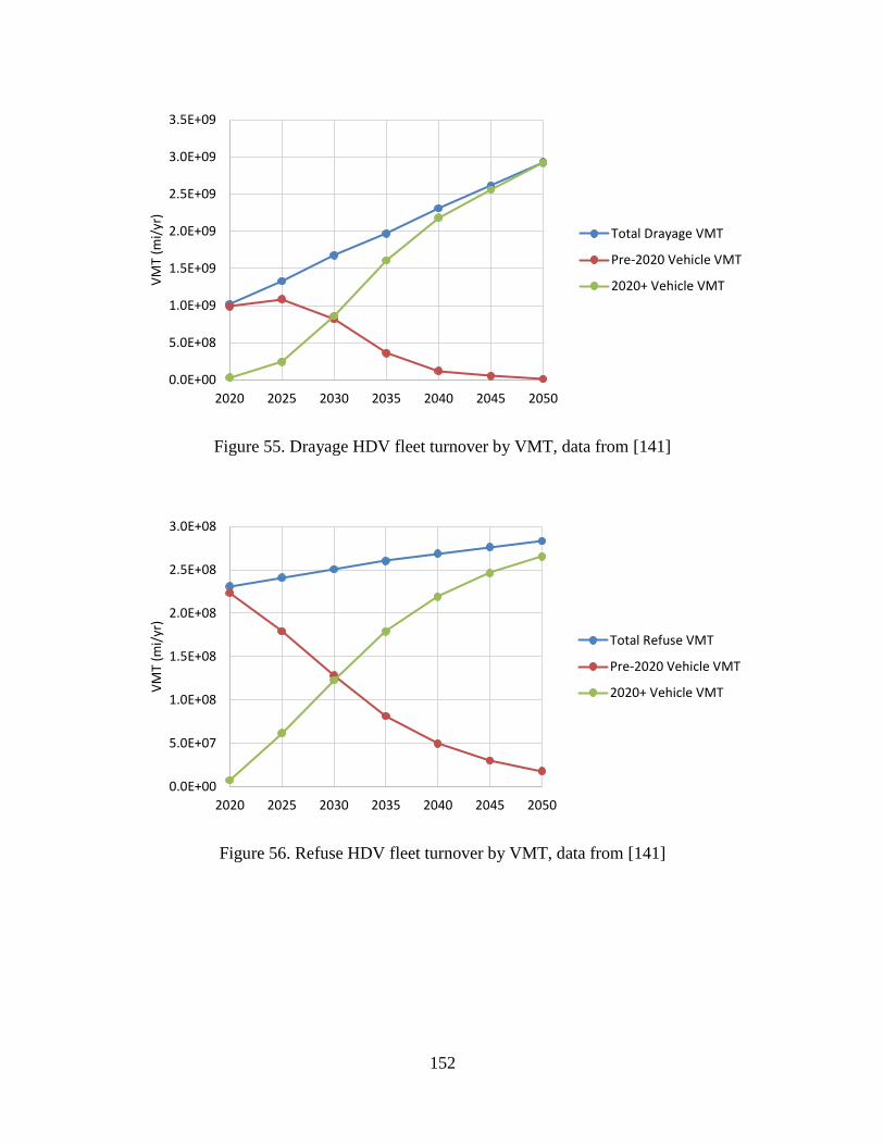
152

Figure 55. Drayage HDV fleet turnover by VMT, data from [141]

Figure 56. Refuse HDV fleet turnover by VMT, data from [141]

0.0E+00

5.0E+08

1.0E+09

1.5E+09

2.0E+09

2.5E+09

3.0E+09

3.5E+09

2020 2025 2030 2035 2040 2045 2050

VM

T (m

i/yr

)

Total Drayage VMT


2020+ Vehicle VMT

0.0E+00

5.0E+07

1.0E+08

1.5E+08

2.0E+08

2.5E+08

3.0E+08

2020 2025 2030 2035 2040 2045 2050

VM

T (m

i/yr

)

Total Refuse VMT


2020+ Vehicle VMT

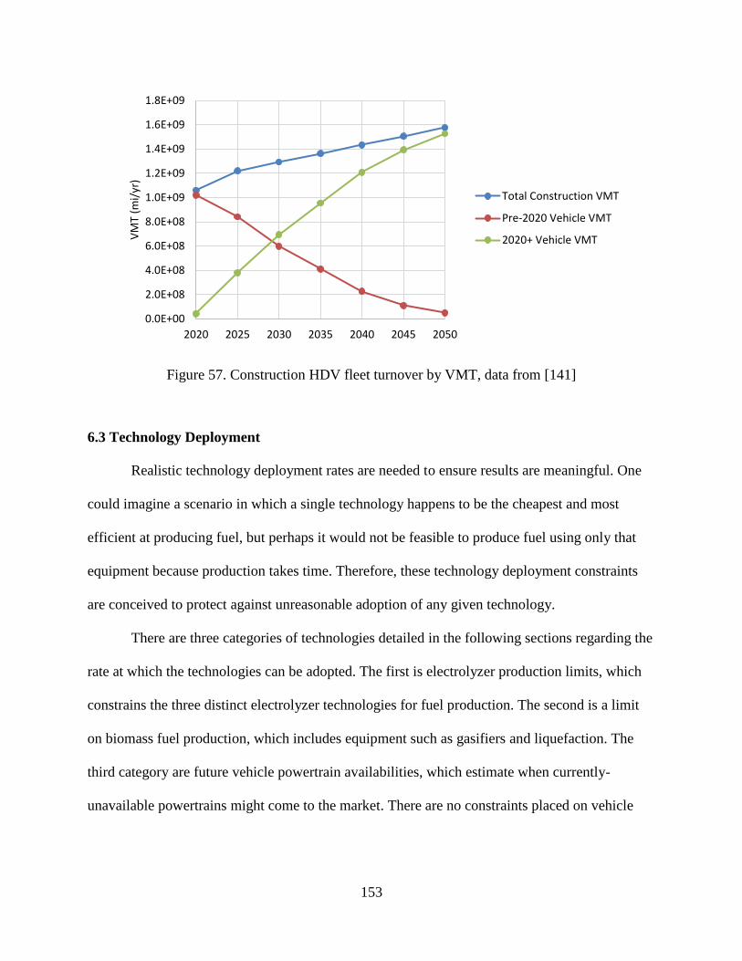
153

Figure 57. Construction HDV fleet turnover by VMT, data from [141]

6.3 Technology Deployment

Realistic technology deployment rates are needed to ensure results are meaningful. One

could imagine a scenario in which a single technology happens to be the cheapest and most

efficient at producing fuel, but perhaps it would not be feasible to produce fuel using only that

equipment because production takes time. Therefore, these technology deployment constraints

are conceived to protect against unreasonable adoption of any given technology.

There are three categories of technologies detailed in the following sections regarding the

rate at which the technologies can be adopted. The first is electrolyzer production limits, which

constrains the three distinct electrolyzer technologies for fuel production. The second is a limit

on biomass fuel production, which includes equipment such as gasifiers and liquefaction. The

third category are future vehicle powertrain availabilities, which estimate when currently-

unavailable powertrains might come to the market. There are no constraints placed on vehicle

0.0E+00

2.0E+08

4.0E+08

6.0E+08

8.0E+08

1.0E+09

1.2E+09

1.4E+09

1.6E+09

1.8E+09

2020 2025 2030 2035 2040 2045 2050

VM

T (m

i/yr

)

Total Construction VMT


2020+ Vehicle VMT

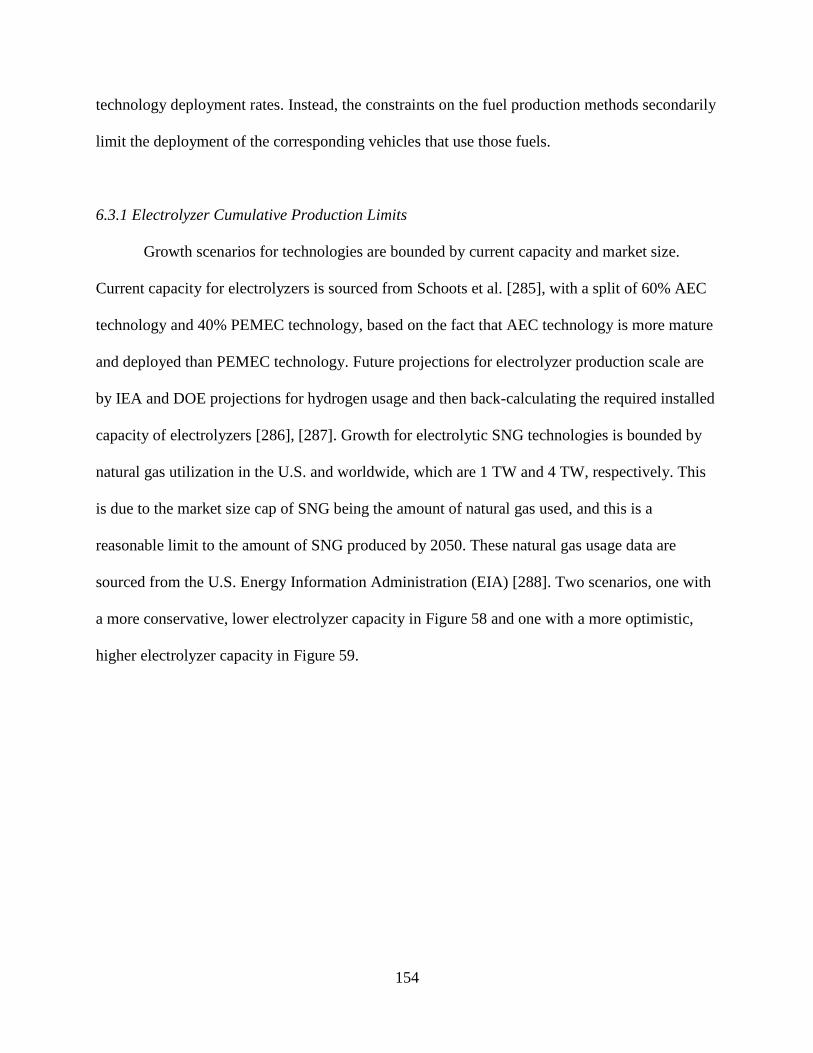
154

technology deployment rates. Instead, the constraints on the fuel production methods secondarily

limit the deployment of the corresponding vehicles that use those fuels.

6.3.1 Electrolyzer Cumulative Production Limits

Growth scenarios for technologies are bounded by current capacity and market size.

Current capacity for electrolyzers is sourced from Schoots et al. [285], with a split of 60% AEC

technology and 40% PEMEC technology, based on the fact that AEC technology is more mature

and deployed than PEMEC technology. Future projections for electrolyzer production scale are

by IEA and DOE projections for hydrogen usage and then back-calculating the required installed

capacity of electrolyzers [286], [287]. Growth for electrolytic SNG technologies is bounded by

natural gas utilization in the U.S. and worldwide, which are 1 TW and 4 TW, respectively. This

is due to the market size cap of SNG being the amount of natural gas used, and this is a

reasonable limit to the amount of SNG produced by 2050. These natural gas usage data are

sourced from the U.S. Energy Information Administration (EIA) [288]. Two scenarios, one with

a more conservative, lower electrolyzer capacity in Figure 58 and one with a more optimistic,

higher electrolyzer capacity in Figure 59.

155

Figure 58. Future electrolyzer market size projections in 2030, 2035, and 2050 (based on

assumed efficiency of 50kWh/kg and capacity factor of 90%)

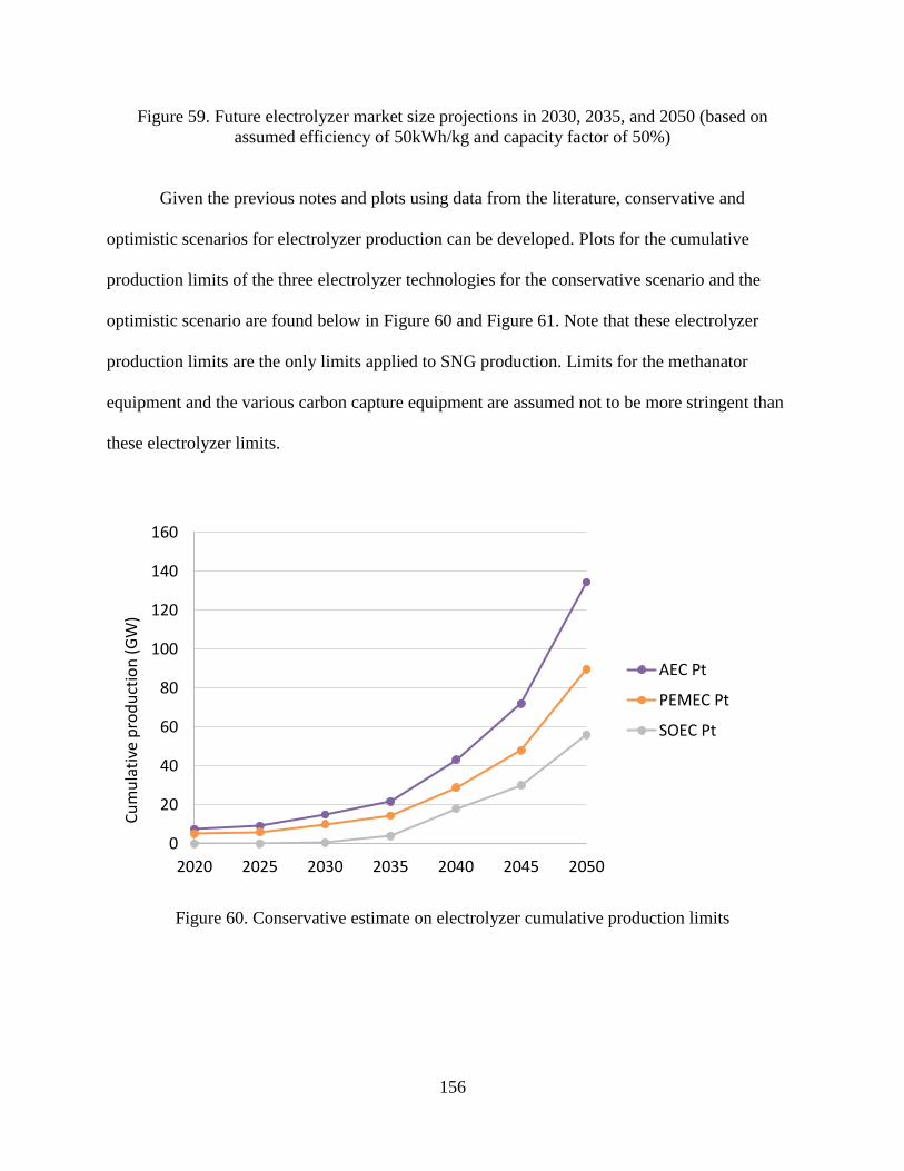
156

Figure 59. Future electrolyzer market size projections in 2030, 2035, and 2050 (based on

assumed efficiency of 50kWh/kg and capacity factor of 50%)

Given the previous notes and plots using data from the literature, conservative and

optimistic scenarios for electrolyzer production can be developed. Plots for the cumulative

production limits of the three electrolyzer technologies for the conservative scenario and the

optimistic scenario are found below in Figure 60 and Figure 61. Note that these electrolyzer

production limits are the only limits applied to SNG production. Limits for the methanator

equipment and the various carbon capture equipment are assumed not to be more stringent than

these electrolyzer limits.

Figure 60. Conservative estimate on electrolyzer cumulative production limits

0

20

40

60

80

100

120

140

160

2020 2025 2030 2035 2040 2045 2050

Cu

mu

lati

ve p

rod

uct

ion

(G

W)

AEC Pt

PEMEC Pt

SOEC Pt

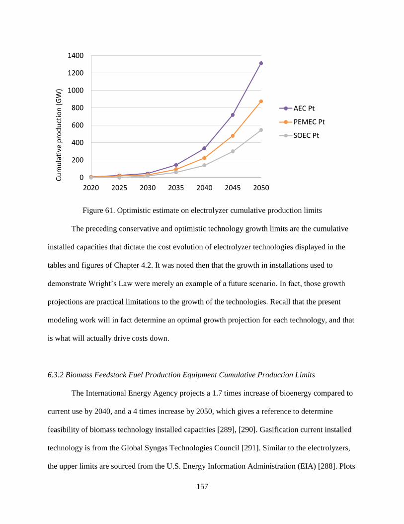
157

Figure 61. Optimistic estimate on electrolyzer cumulative production limits

The preceding conservative and optimistic technology growth limits are the cumulative

installed capacities that dictate the cost evolution of electrolyzer technologies displayed in the

tables and figures of Chapter 4.2. It was noted then that the growth in installations used to

demonstrate Wright’s Law were merely an example of a future scenario. In fact, those growth

projections are practical limitations to the growth of the technologies. Recall that the present

modeling work will in fact determine an optimal growth projection for each technology, and that

is what will actually drive costs down.

6.3.2 Biomass Feedstock Fuel Production Equipment Cumulative Production Limits

The International Energy Agency projects a 1.7 times increase of bioenergy compared to

current use by 2040, and a 4 times increase by 2050, which gives a reference to determine

feasibility of biomass technology installed capacities [289], [290]. Gasification current installed

technology is from the Global Syngas Technologies Council [291]. Similar to the electrolyzers,

the upper limits are sourced from the U.S. Energy Information Administration (EIA) [288]. Plots

0

200

400

600

800

1000

1200

1400

2020 2025 2030 2035 2040 2045 2050

Cu

mu

lati

ve p

rod

uct

ion

(G

W)

AEC Pt

PEMEC Pt

SOEC Pt

158

for the cumulative production limits of gasifiers, AD, gasifier-FT, hydrolysis, pyrolysis, and

liquefaction are shown in Figure 62. Note that unlike the electrolyzers, which are more

technically advanced and complicated than the biomass conversion processes as well as having

less data in the literature, there are no conservative and optimistic projections; there is simply

one projection.

Figure 62. Biomass feedstock fuel production equipment cumulative production limits

As with the electrolyzer technologies, the preceding growth limits are what were displayed for

the various biomass fuel production technologies in Chapter 4.2.

6.3.3 Future Vehicle Powertrain Availabilities

For LDVs, all of the powertrain configurations in this analysis are currently available

except PFCEVs. However, at least one manufacturer has begun preparing for series production

of a PFCEV, with the intention of selling it soon [160]. Therefore, this work assumes that

PFCEVs will be available by 2020, for the first year of modeling.

0

200

400

600

800

1000

1200

2020 2025 2030 2035 2040 2045 2050

Cu

mu

lati

ve p

rod

uct

ion

(G

Wth

)

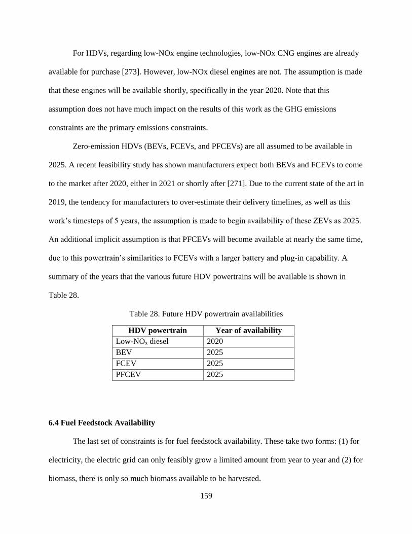
159

For HDVs, regarding low-NOx engine technologies, low-NOx CNG engines are already

available for purchase [273]. However, low-NOx diesel engines are not. The assumption is made

that these engines will be available shortly, specifically in the year 2020. Note that this

assumption does not have much impact on the results of this work as the GHG emissions

constraints are the primary emissions constraints.

Zero-emission HDVs (BEVs, FCEVs, and PFCEVs) are all assumed to be available in

2025. A recent feasibility study has shown manufacturers expect both BEVs and FCEVs to come

to the market after 2020, either in 2021 or shortly after [271]. Due to the current state of the art in

2019, the tendency for manufacturers to over-estimate their delivery timelines, as well as this

work’s timesteps of 5 years, the assumption is made to begin availability of these ZEVs as 2025.

An additional implicit assumption is that PFCEVs will become available at nearly the same time,

due to this powertrain’s similarities to FCEVs with a larger battery and plug-in capability. A

summary of the years that the various future HDV powertrains will be available is shown in

Table 28.

Table 28. Future HDV powertrain availabilities

HDV powertrain Year of availability

Low-NOx diesel 2020

BEV 2025

FCEV 2025

PFCEV 2025

6.4 Fuel Feedstock Availability

The last set of constraints is for fuel feedstock availability. These take two forms: (1) for

electricity, the electric grid can only feasibly grow a limited amount from year to year and (2) for

biomass, there is only so much biomass available to be harvested.

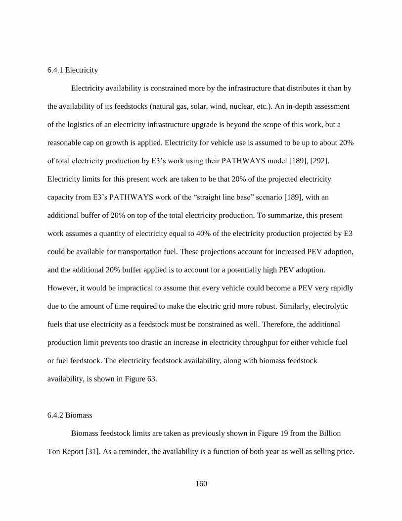
160

6.4.1 Electricity

Electricity availability is constrained more by the infrastructure that distributes it than by

the availability of its feedstocks (natural gas, solar, wind, nuclear, etc.). An in-depth assessment

of the logistics of an electricity infrastructure upgrade is beyond the scope of this work, but a

reasonable cap on growth is applied. Electricity for vehicle use is assumed to be up to about 20%

of total electricity production by E3’s work using their PATHWAYS model [189], [292].

Electricity limits for this present work are taken to be that 20% of the projected electricity

capacity from E3’s PATHWAYS work of the “straight line base” scenario [189], with an

additional buffer of 20% on top of the total electricity production. To summarize, this present

work assumes a quantity of electricity equal to 40% of the electricity production projected by E3

could be available for transportation fuel. These projections account for increased PEV adoption,

and the additional 20% buffer applied is to account for a potentially high PEV adoption.

However, it would be impractical to assume that every vehicle could become a PEV very rapidly

due to the amount of time required to make the electric grid more robust. Similarly, electrolytic

fuels that use electricity as a feedstock must be constrained as well. Therefore, the additional

production limit prevents too drastic an increase in electricity throughput for either vehicle fuel

or fuel feedstock. The electricity feedstock availability, along with biomass feedstock

availability, is shown in Figure 63.

6.4.2 Biomass

Biomass feedstock limits are taken as previously shown in Figure 19 from the Billion

Ton Report [31]. As a reminder, the availability is a function of both year as well as selling price.

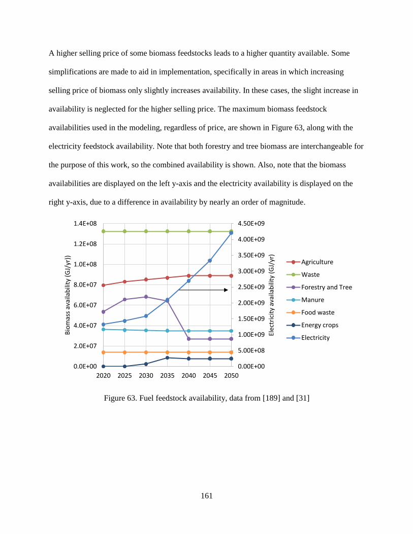
161

A higher selling price of some biomass feedstocks leads to a higher quantity available. Some

simplifications are made to aid in implementation, specifically in areas in which increasing

selling price of biomass only slightly increases availability. In these cases, the slight increase in

availability is neglected for the higher selling price. The maximum biomass feedstock

availabilities used in the modeling, regardless of price, are shown in Figure 63, along with the

electricity feedstock availability. Note that both forestry and tree biomass are interchangeable for

the purpose of this work, so the combined availability is shown. Also, note that the biomass

availabilities are displayed on the left y-axis and the electricity availability is displayed on the

right y-axis, due to a difference in availability by nearly an order of magnitude.

Figure 63. Fuel feedstock availability, data from [189] and [31]

0.00E+00

5.00E+08

1.00E+09

1.50E+09

2.00E+09

2.50E+09

3.00E+09

3.50E+09

4.00E+09

4.50E+09

0.0E+00

2.0E+07

4.0E+07

6.0E+07

8.0E+07

1.0E+08

1.2E+08

1.4E+08

2020 2025 2030 2035 2040 2045 2050

Elec

tric

ity

avai

lab

ility

(G

J/yr

)

Bio

mas

s av

aila

bili

ty (

GJ/

yr))

Agriculture

Waste

Forestry and Tree

Manure

Food waste

Energy crops

Electricity

162

7. ESTABLISHING THE OPTIMIZATION PROBLEM

The various components of the chain from fuel production to vehicles have been

analyzed for efficiency, emissions, and cost; and Wright’s Law has been identified as the

methodology of projecting these costs into the future. With these data, it is now possible to

calculate the total cost of each potential pathway. Additionally, the various constraints of the

problem have been detailed. This chapter is devoted to describing how these costs and

constraints are implemented into a formal optimization problem for the timeframe of 2020 (the

near future) into 2050.

The modeling tool developed to solve the goal of this dissertation is christened

Transportation Affecting Cost and Emissions (TRACE). The model, including projections and

optimization, will hereafter be referred to as TRACE.

7.1 Optimization Method

Given the techno-economic data and constraints, it is evident that LP is an appropriate

optimization tool for TRACE. One could argue that MILP is most appropriate as there can

realistically only be an integer number of vehicles. However, given the scale of the problem

being solved, approximating the number of vehicles chosen by this optimization as a continuous

variable will not lead to any significant difference in results (2.9E10 new LDV miles traveled in

2020 with an average annual mileage of 11,346 miles per vehicle [140] leads to about 2.6 million

LDVs in 2030; the same methodology for the HDV vocations leads to at least 166 vehicles being

chosen, assumed to be a sufficiently large quantity that integer numbers are unnecessary for the

results expected). Additionally, as there is no explicit spatial consideration in this work,

individual fueling stations are not considered, but instead analyzed as a continuous quantity of

163

fuel being distributed and dispensed with costs varying continuously as well. Therefore, there is

no need to incur the added computational burden of modeling this problem as a MILP problem.

IBM’s CPLEX software integrates well with MATLAB, so it is the software of choice.

Additionally, the MATLAB toolbox YALMIP is used to set up the constraints of the

optimization problem [293].

The variables that describe this problem are the fuel pathways and the vehicle types. Fuel

pathways are differentiated by feedstock (and, when appropriate, feedstock separated by distinct

selling price) and fuel production technology. Vehicles are differentiated by LDVs and each of

the HDV vocations for all appropriate vehicle powertrain configurations. This leads to a total of

151 variables, 109 of which are for fuel production and 42 are for vehicles.

7.2 Cost Function

The cost function of TRACE is determined by the techno-economic data gathered and

projection methods described in Chapters 4 and 5. Each fuel pathway and corresponding vehicle

powertrain configuration will have an associated cost per amount of energy of fuel and

correspondingly number of vehicles.

The cost function is generally split into two categories: (1) fuel feedstock, production,

distribution, and dispensing; and (2) vehicles. The reason for this splitting is some fuels can be

used in multiple vehicles. Separating into the two categories allows the modeling to

independently select fuel production pathway and vehicle type without having to code each and

every potential fuel and vehicle pathway. Note that a modeling constraint, to be introduced

shortly, links the fuel variables to the vehicle variables.

164

One exception to the above is for PEVs. For PEVs, the electricity feedstock cost is

calculated separately and both electricity distribution and dispensing costs are lumped with the

PEV cost (recall that electricity production costs are incorporated into the feedstock cost). This is

because electricity distribution and dispensing costs are dependent upon the level of charging

power required by the PEV as noted in Chapter 4.4.1. For example, light-duty PHEVs and

PFCEVs only require level 1 charging. Therefore, distribution costs are assumed negligible for

these vehicles and dispensing costs are much lower than scenarios that require level 2 or level 3

dispensing. Due to these infrastructure cost differences, the distribution and dispensing costs are

grouped with the vehicle cost so the appropriate numbers are used.

The TRACE cost function is presented in Equation 13. This cost function is minimized

for each timestep (i.e. 2020 to 2050 in five year increments). After each timestep, costs and

efficiencies are updated as noted in the last section of this chapter.

165

Equation 13. TRACE cost function

min

(

∑

(

𝑓𝑒𝑒𝑑𝑠𝑡𝑜𝑐𝑘𝑖,𝑡 +

((𝑝𝑟𝑜𝑑𝑢𝑐𝑡𝑖𝑜𝑛𝑗,𝑡 ∗ 𝐶𝑅𝐹) + 𝐹𝑂𝑀𝑗

𝐶𝐹𝑖 ∗ 8760ℎ𝑦𝑟

+ 𝑉𝑂𝑀𝑗)

0.0036𝐺𝐽𝑘𝑊ℎ

𝜂𝑝𝑟𝑜𝑑𝑢𝑐𝑡𝑖𝑜𝑛,𝑗,𝑡 ∗ 𝜂𝑑𝑖𝑠𝑡𝑟𝑖𝑏𝑢𝑡𝑖𝑜𝑛,𝑘 ∗ 𝜂𝑑𝑖𝑠𝑝𝑒𝑛𝑠𝑖𝑛𝑔,𝑚+𝑑𝑖𝑠𝑡𝑟𝑖𝑏𝑢𝑡𝑖𝑜𝑛𝑘𝜂𝑑𝑖𝑠𝑝𝑒𝑛𝑠𝑖𝑛𝑔,𝑚

𝑖,𝑗,𝑘,𝑚,𝑡

+ 𝑑𝑖𝑠𝑝𝑒𝑛𝑠𝑖𝑛𝑔𝑚

)

∗ 𝑥𝑛,𝑡 + ∑ (𝑣𝑒ℎ𝑖𝑐𝑙𝑒𝑝,𝑡 ∗ 𝐶𝑅𝐹

𝑎𝑎𝑉𝑀𝑇𝑞) ∗ 𝑦𝑝,𝑡

𝑝,𝑞,𝑡

)

The sets, variables, and parameters used in Equation 13 are described in Table 29.

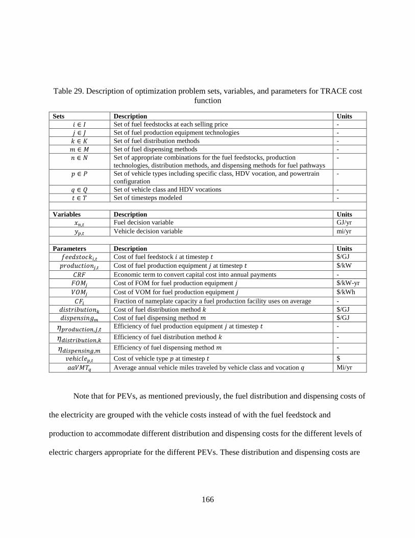
166

Table 29. Description of optimization problem sets, variables, and parameters for TRACE cost

function

Sets Description Units

𝑖 ∈ 𝐼 Set of fuel feedstocks at each selling price -

𝑗 ∈ 𝐽 Set of fuel production equipment technologies -

𝑘 ∈ 𝐾 Set of fuel distribution methods -

𝑚 ∈ 𝑀 Set of fuel dispensing methods -

𝑛 ∈ 𝑁 Set of appropriate combinations for the fuel feedstocks, production

technologies, distribution methods, and dispensing methods for fuel pathways

-

𝑝 ∈ 𝑃 Set of vehicle types including specific class, HDV vocation, and powertrain

configuration

-

𝑞 ∈ 𝑄 Set of vehicle class and HDV vocations -

𝑡 ∈ 𝑇 Set of timesteps modeled -

Variables Description Units

𝑥𝑛,𝑡 Fuel decision variable GJ/yr

𝑦𝑝,𝑡 Vehicle decision variable mi/yr

Parameters Description Units

𝑓𝑒𝑒𝑑𝑠𝑡𝑜𝑐𝑘𝑖,𝑡 Cost of fuel feedstock 𝑖 at timestep 𝑡 $/GJ

𝑝𝑟𝑜𝑑𝑢𝑐𝑡𝑖𝑜𝑛𝑗,𝑡 Cost of fuel production equipment 𝑗 at timestep 𝑡 $/kW

𝐶𝑅𝐹 Economic term to convert capital cost into annual payments -

𝐹𝑂𝑀𝑗 Cost of FOM for fuel production equipment 𝑗 $/kW-yr

𝑉𝑂𝑀𝑗 Cost of VOM for fuel production equipment 𝑗 $/kWh

𝐶𝐹𝑖 Fraction of nameplate capacity a fuel production facility uses on average -

𝑑𝑖𝑠𝑡𝑟𝑖𝑏𝑢𝑡𝑖𝑜𝑛𝑘 Cost of fuel distribution method 𝑘 $/GJ

𝑑𝑖𝑠𝑝𝑒𝑛𝑠𝑖𝑛𝑔𝑚 Cost of fuel dispensing method 𝑚 $/GJ

𝜂𝑝𝑟𝑜𝑑𝑢𝑐𝑡𝑖𝑜𝑛,𝑗,𝑡 Efficiency of fuel production equipment 𝑗 at timestep 𝑡 -

𝜂𝑑𝑖𝑠𝑡𝑟𝑖𝑏𝑢𝑡𝑖𝑜𝑛,𝑘 Efficiency of fuel distribution method 𝑘 -

𝜂𝑑𝑖𝑠𝑝𝑒𝑛𝑠𝑖𝑛𝑔,𝑚 Efficiency of fuel dispensing method 𝑚 -

𝑣𝑒ℎ𝑖𝑐𝑙𝑒𝑝,𝑡 Cost of vehicle type 𝑝 at timestep 𝑡 $

𝑎𝑎𝑉𝑀𝑇𝑞 Average annual vehicle miles traveled by vehicle class and vocation 𝑞 Mi/yr

Note that for PEVs, as mentioned previously, the fuel distribution and dispensing costs of

the electricity are grouped with the vehicle costs instead of with the fuel feedstock and

production to accommodate different distribution and dispensing costs for the different levels of

electric chargers appropriate for the different PEVs. These distribution and dispensing costs are

167

divided by the PEV’s CD efficiency to convert from cost on a per mile energy basis to a per mile

basis for consistency with the vehicle cost.

Both electrolytic fuels and biomass fuels can have different capacity factors, which could

affect the cost of the associated fuel. For electrolytic fuels is a high capacity factor of 0.8, which

depicts a scenario in which P2G is run nearly continually to maximize the usage and fuel output.

This is most appropriate for use with the distribution electricity grid with a mix of both

renewable and non-renewable resources, which fits the data from E3 detailed in Chapter 4.1.1.

Using the high capacity factor decreases capital cost of fuel production equipment compared to

fuel output. For biomass feedstocks, a 0.8 capacity factor is also used, assuming a relatively high

biomass throughput to capitalize on the biofuel production plants purchased but also allowing for

downtime of repairs and other necessary upkeep. Later scenarios detailed in Chapter 8 will

determine the effect of capacity factor on cost, which is most relevant for electrolytic fuels due to

the decreased cost of electricity that could accompany a low-capacity factor P2G plant. Biomass

cost is not as dependent on capacity factor as electricity cost is.

7.3 Constraints

The emissions regulations, VMT requirements, realistic technology growth rates, and

feedstock availability from Chapter 6 compose the major constraints of TRACE. These and the

rest of the constraints included are given in Equation 14 through Equation 22.

The first constraint, Equation 14, ensures that both fuel production and vehicle adoption

are positive and finite values to ensure they make physical sense.

Equation 14. Constraint: Positive and finite values for fuel production and vehicle adoption

0 ≤ 𝑥𝑛,𝑡, 𝑦𝑝,𝑡 ≤ 1𝑒15

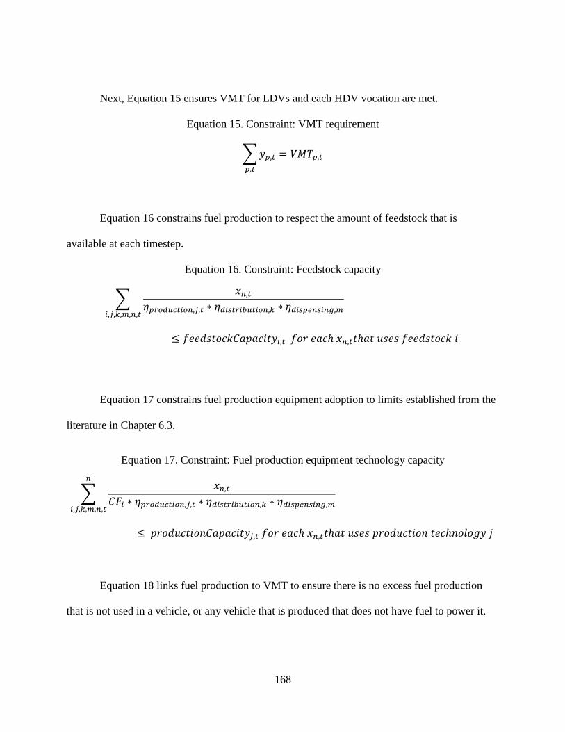
168

Next, Equation 15 ensures VMT for LDVs and each HDV vocation are met.

Equation 15. Constraint: VMT requirement

∑𝑦𝑝,𝑡 = 𝑉𝑀𝑇𝑝,𝑡

𝑝,𝑡

Equation 16 constrains fuel production to respect the amount of feedstock that is

available at each timestep.

Equation 16. Constraint: Feedstock capacity

∑𝑥𝑛,𝑡

𝜂𝑝𝑟𝑜𝑑𝑢𝑐𝑡𝑖𝑜𝑛,𝑗,𝑡 ∗ 𝜂𝑑𝑖𝑠𝑡𝑟𝑖𝑏𝑢𝑡𝑖𝑜𝑛,𝑘 ∗ 𝜂𝑑𝑖𝑠𝑝𝑒𝑛𝑠𝑖𝑛𝑔,𝑚

𝑖,𝑗,𝑘,𝑚,𝑛,𝑡

≤ 𝑓𝑒𝑒𝑑𝑠𝑡𝑜𝑐𝑘𝐶𝑎𝑝𝑎𝑐𝑖𝑡𝑦𝑖,𝑡 𝑓𝑜𝑟 𝑒𝑎𝑐ℎ 𝑥𝑛,𝑡𝑡ℎ𝑎𝑡 𝑢𝑠𝑒𝑠 𝑓𝑒𝑒𝑑𝑠𝑡𝑜𝑐𝑘 𝑖

Equation 17 constrains fuel production equipment adoption to limits established from the

literature in Chapter 6.3.

Equation 17. Constraint: Fuel production equipment technology capacity

∑𝑥𝑛,𝑡

𝐶𝐹𝑖 ∗ 𝜂𝑝𝑟𝑜𝑑𝑢𝑐𝑡𝑖𝑜𝑛,𝑗,𝑡 ∗ 𝜂𝑑𝑖𝑠𝑡𝑟𝑖𝑏𝑢𝑡𝑖𝑜𝑛,𝑘 ∗ 𝜂𝑑𝑖𝑠𝑝𝑒𝑛𝑠𝑖𝑛𝑔,𝑚

𝑛

𝑖,𝑗,𝑘,𝑚,𝑛,𝑡

≤ 𝑝𝑟𝑜𝑑𝑢𝑐𝑡𝑖𝑜𝑛𝐶𝑎𝑝𝑎𝑐𝑖𝑡𝑦𝑗,𝑡 𝑓𝑜𝑟 𝑒𝑎𝑐ℎ 𝑥𝑛,𝑡𝑡ℎ𝑎𝑡 𝑢𝑠𝑒𝑠 𝑝𝑟𝑜𝑑𝑢𝑐𝑡𝑖𝑜𝑛 𝑡𝑒𝑐ℎ𝑛𝑜𝑙𝑜𝑔𝑦 𝑗

Equation 18 links fuel production to VMT to ensure there is no excess fuel production

that is not used in a vehicle, or any vehicle that is produced that does not have fuel to power it.

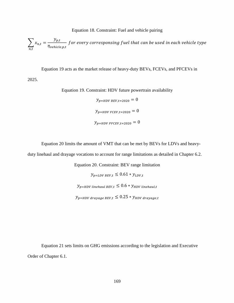
169

Equation 18. Constraint: Fuel and vehicle pairing

∑𝑥𝑛,𝑡 =𝑦𝑝,𝑡

𝜂𝑣𝑒ℎ𝑖𝑐𝑙𝑒,𝑝,𝑡

𝑛,𝑡

𝑓𝑜𝑟 𝑒𝑣𝑒𝑟𝑦 𝑐𝑜𝑟𝑟𝑒𝑠𝑝𝑜𝑛𝑠𝑖𝑛𝑔 𝑓𝑢𝑒𝑙 𝑡ℎ𝑎𝑡 𝑐𝑎𝑛 𝑏𝑒 𝑢𝑠𝑒𝑑 𝑖𝑛 𝑒𝑎𝑐ℎ 𝑣𝑒ℎ𝑖𝑐𝑙𝑒 𝑡𝑦𝑝𝑒

Equation 19 acts as the market release of heavy-duty BEVs, FCEVs, and PFCEVs in

2025.

Equation 19. Constraint: HDV future powertrain availability

𝑦𝑝=𝐻𝐷𝑉 𝐵𝐸𝑉,𝑡=2020 = 0

𝑦𝑝=𝐻𝐷𝑉 𝐹𝐶𝐸𝑉,𝑡=2020 = 0

𝑦𝑝=𝐻𝐷𝑉 𝑃𝐹𝐶𝐸𝑉,𝑡=2020 = 0

Equation 20 limits the amount of VMT that can be met by BEVs for LDVs and heavy-

duty linehaul and drayage vocations to account for range limitations as detailed in Chapter 6.2.

Equation 20. Constraint: BEV range limitation

𝑦𝑝=𝐿𝐷𝑉 𝐵𝐸𝑉,𝑡 ≤ 0.61 ∗ 𝑦𝐿𝐷𝑉,𝑡

𝑦𝑝=𝐻𝐷𝑉 𝑙𝑖𝑛𝑒ℎ𝑎𝑢𝑙 𝐵𝐸𝑉,𝑡 ≤ 0.6 ∗ 𝑦𝐻𝐷𝑉 𝑙𝑖𝑛𝑒ℎ𝑎𝑢𝑙,𝑡

𝑦𝑝=𝐻𝐷𝑉 𝑑𝑟𝑎𝑦𝑎𝑔𝑒 𝐵𝐸𝑉,𝑡 ≤ 0.25 ∗ 𝑦𝐻𝐷𝑉 𝑑𝑟𝑎𝑦𝑎𝑔𝑒,𝑡

Equation 21 sets limits on GHG emissions according to the legislation and Executive

Order of Chapter 6.1.

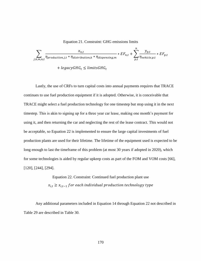
170

Equation 21. Constraint: GHG emissions limits

∑𝑥𝑛,𝑡

𝜂𝑝𝑟𝑜𝑑𝑢𝑐𝑡𝑖𝑜𝑛,𝑗,𝑡 ∗ 𝜂𝑑𝑖𝑠𝑡𝑟𝑖𝑏𝑢𝑡𝑖𝑜𝑛,𝑘 ∗ 𝜂𝑑𝑖𝑠𝑝𝑒𝑛𝑠𝑖𝑛𝑔,𝑚

𝑗,𝑘,𝑚,𝑛,𝑡

∗ 𝐸𝐹𝑛,𝑡 +∑𝑦𝑝,𝑡

𝜂𝑣𝑒ℎ𝑖𝑐𝑙𝑒,𝑝,𝑡

𝑛

𝑝,𝑡

∗ 𝐸𝐹𝑝,𝑡

+ 𝑙𝑒𝑔𝑎𝑐𝑦𝐺𝐻𝐺𝑡 ≤ 𝑙𝑖𝑚𝑖𝑡𝑠𝐺𝐻𝐺𝑡

Lastly, the use of CRFs to turn capital costs into annual payments requires that TRACE

continues to use fuel production equipment if it is adopted. Otherwise, it is conceivable that

TRACE might select a fuel production technology for one timestep but stop using it in the next

timestep. This is akin to signing up for a three year car lease, making one month’s payment for

using it, and then returning the car and neglecting the rest of the lease contract. This would not

be acceptable, so Equation 22 is implemented to ensure the large capital investments of fuel

production plants are used for their lifetime. The lifetime of the equipment used is expected to be

long enough to last the timeframe of this problem (at most 30 years if adopted in 2020), which

for some technologies is aided by regular upkeep costs as part of the FOM and VOM costs [66],

[120], [244], [294].

Equation 22. Constraint: Continued fuel production plant use

𝑥𝑖,𝑡 ≥ 𝑥𝑖,𝑡−1 𝑓𝑜𝑟 𝑒𝑎𝑐ℎ 𝑖𝑛𝑑𝑖𝑣𝑖𝑑𝑢𝑎𝑙 𝑝𝑟𝑜𝑑𝑢𝑐𝑡𝑖𝑜𝑛 𝑡𝑒𝑐ℎ𝑛𝑜𝑙𝑜𝑔𝑦 𝑡𝑦𝑝𝑒

Any additional parameters included in Equation 14 through Equation 22 not described in

Table 29 are described in Table 30.

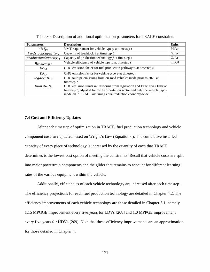
171

Table 30. Description of additional optimization parameters for TRACE constraints

Parameters Description Units

𝑉𝑀𝑇𝑝,𝑡 VMT requirement for vehicle type 𝑝 at timestep 𝑡 Mi/yr

𝑓𝑒𝑒𝑑𝑠𝑡𝑜𝑐𝑘𝐶𝑎𝑝𝑎𝑐𝑖𝑡𝑦𝑖,𝑡 Capacity of feedstock 𝑖 at timestep 𝑡 GJ/yr

𝑝𝑟𝑜𝑑𝑢𝑐𝑡𝑖𝑜𝑛𝐶𝑎𝑝𝑎𝑐𝑖𝑡𝑦𝑗,𝑡 Capacity of production technology 𝑗 at timestep 𝑡 GJ/yr

𝜂𝑣𝑒ℎ𝑖𝑐𝑙𝑒,𝑝,𝑡 Vehicle efficiency of vehicle type 𝑝 at timestep 𝑡 mi/GJ

𝐸𝐹𝑛,𝑡 GHG emission factor for fuel production pathway 𝑛 at timestep 𝑡

𝐸𝐹𝑝,𝑡 GHG emission factor for vehicle type 𝑝 at timestep 𝑡

𝑙𝑒𝑔𝑎𝑐𝑦𝐺𝐻𝐺𝑡 GHG tailpipe emissions from on-road vehicles made prior to 2020 at

timestep 𝑡

𝑙𝑖𝑚𝑖𝑡𝑠𝐺𝐻𝐺𝑡 GHG emission limits in California from legislation and Executive Order at

timestep 𝑡, adjusted for the transportation sector and only the vehicle types

modeled in TRACE assuming equal reduction economy-wide

7.4 Cost and Efficiency Updates

After each timestep of optimization in TRACE, fuel production technology and vehicle

component costs are updated based on Wright’s Law (Equation 6). The cumulative installed

capacity of every piece of technology is increased by the quantity of each that TRACE

determines is the lowest cost option of meeting the constraints. Recall that vehicle costs are split

into major powertrain components and the glider that remains to account for different learning

rates of the various equipment within the vehicle.

Additionally, efficiencies of each vehicle technology are increased after each timestep.

The efficiency projections for each fuel production technology are detailed in Chapter 4.2. The

efficiency improvements of each vehicle technology are those detailed in Chapter 5.1, namely

1.15 MPGGE improvement every five years for LDVs [268] and 1.0 MPPGE improvement

every five years for HDVs [269]. Note that these efficiency improvements are an approximation

for those detailed in Chapter 4.

172

8. OPTIMAL FUEL AND VEHICLE DEPLOYMENT

This chapter analyzes the Reference Case, which is included to have a comparison for

TRACE results, as well as the TRACE results. Default parameters are used at first for a baseline

result of what future transportation sector could look like when adopting clean fuels and meeting

all constraints outlined in Chapter 7.3. Additionally, some additional constraints are imposed and

several sensitivity analyses are conducted to exercise TRACE in interesting ways and gather

insight into factors that affect transportation technology evolution.

8.1 Reference Case

The Reference Case which serves as a comparison for TRACE optimization results uses

conventional fossil gasoline, diesel, and natural gas as fuels and ICVs for all vehicle types. For

this Reference Case, all LDVs use gasoline as fuel, 47% of refuse HDVs use natural gas as found

in EMFAC 2020 projections [141], and the rest of the refuse HDVs as well as all other vocations

of HDVs use diesel.

The Reference Case handles vehicle efficiency and cost the same as detailed for TRACE.

All ICVs have the same improved efficiencies over time as described in Chapter 5.1 and Chapter

7.4. The Reference Case uses the same starting cost of ICVs as detailed in Chapter 5.2 and

applies Wright’s Law on each vehicle component based on cumulative production for vehicle

cost reductions. Emissions for the gasoline, diesel, and natural gas used in ICVs are from the

GREET WTW Calculator [295]. This tool lists the WTW emissions for the fossil fuels of

interest. These data are gathered on a per-energy basis so the modeled ICV efficiency can be

incorporated.

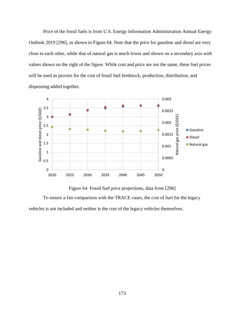
173

Price of the fossil fuels is from U.S. Energy Information Administration Annual Energy

Outlook 2019 [296], as shown in Figure 64. Note that the price for gasoline and diesel are very

close to each other, while that of natural gas is much lower and shown on a secondary axis with

values shown on the right of the figure. While cost and price are not the same, these fuel prices

will be used as proxies for the cost of fossil fuel feedstock, production, distribution, and

dispensing added together.

Figure 64. Fossil fuel price projections, data from [296]

To ensure a fair comparison with the TRACE cases, the cost of fuel for the legacy

vehicles is not included and neither is the cost of the legacy vehicles themselves.

0

0.0005

0.001

0.0015

0.002

0.0025

0.003

0

0.5

1

1.5

2

2.5

3

3.5

4

2020 2025 2030 2035 2040 2045 2050N

atu

ral g

as p

rice

($

/GG

E)

Gas

olin

e an

d d

iese

l pri

ce (

$/G

GE)

Gasoline

Diesel

Natural gas

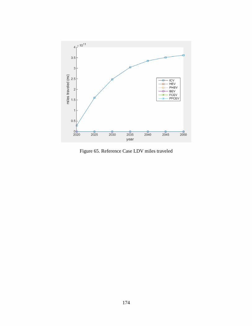
174

Figure 65. Reference Case LDV miles traveled

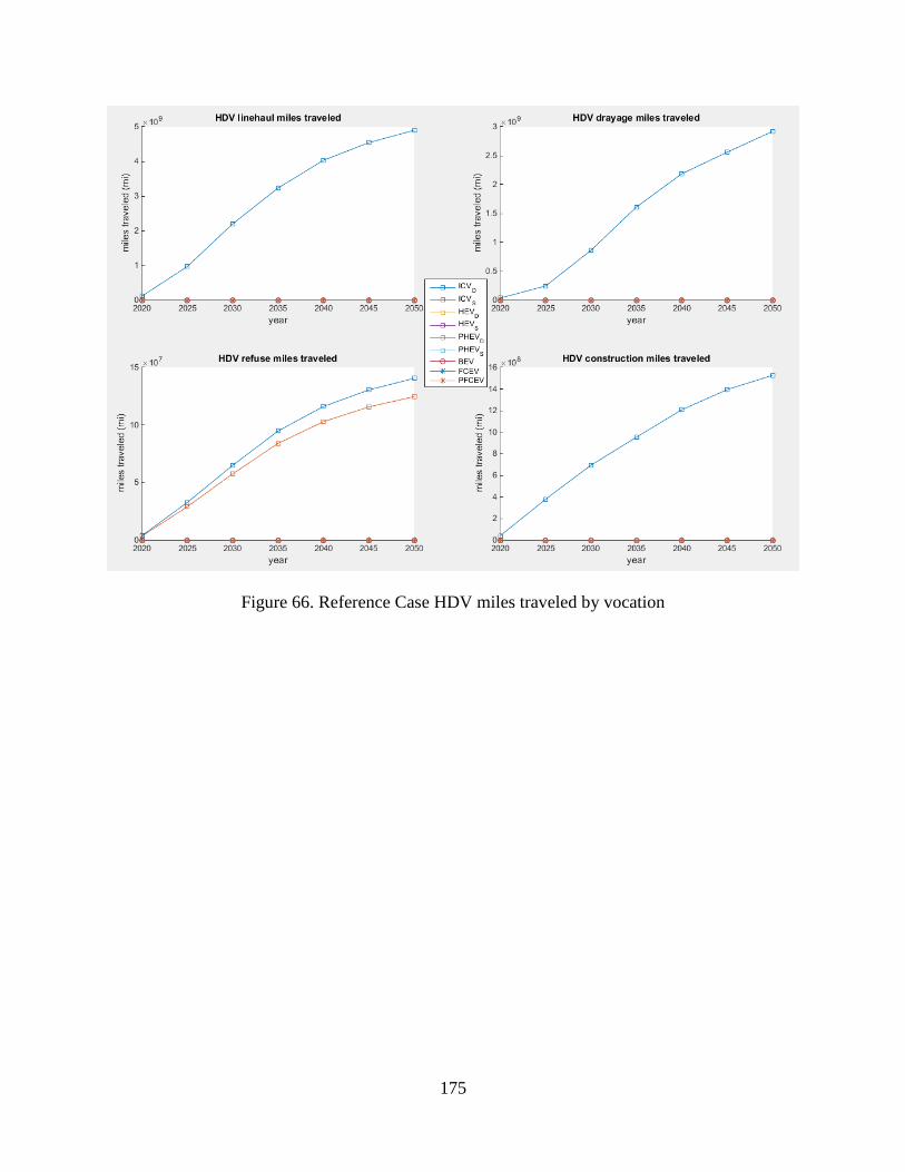
175

Figure 66. Reference Case HDV miles traveled by vocation

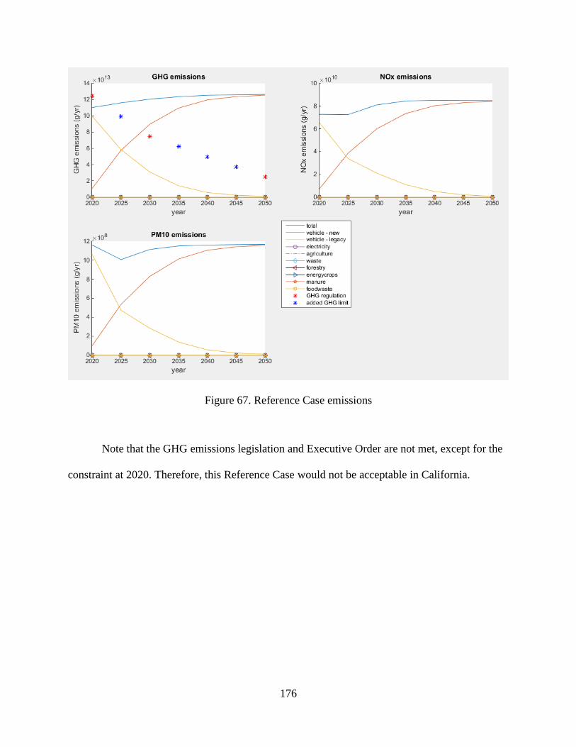
176

Figure 67. Reference Case emissions

Note that the GHG emissions legislation and Executive Order are not met, except for the

constraint at 2020. Therefore, this Reference Case would not be acceptable in California.

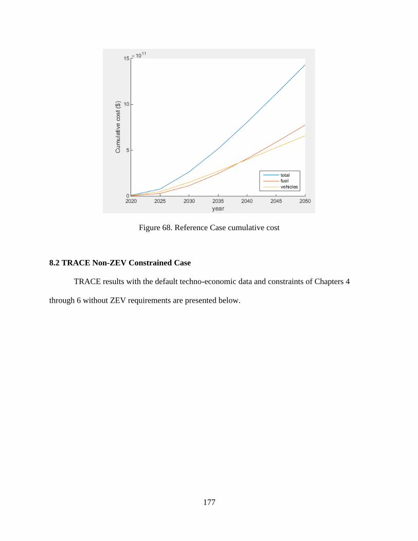
177

Figure 68. Reference Case cumulative cost

8.2 TRACE Non-ZEV Constrained Case

TRACE results with the default techno-economic data and constraints of Chapters 4

through 6 without ZEV requirements are presented below.

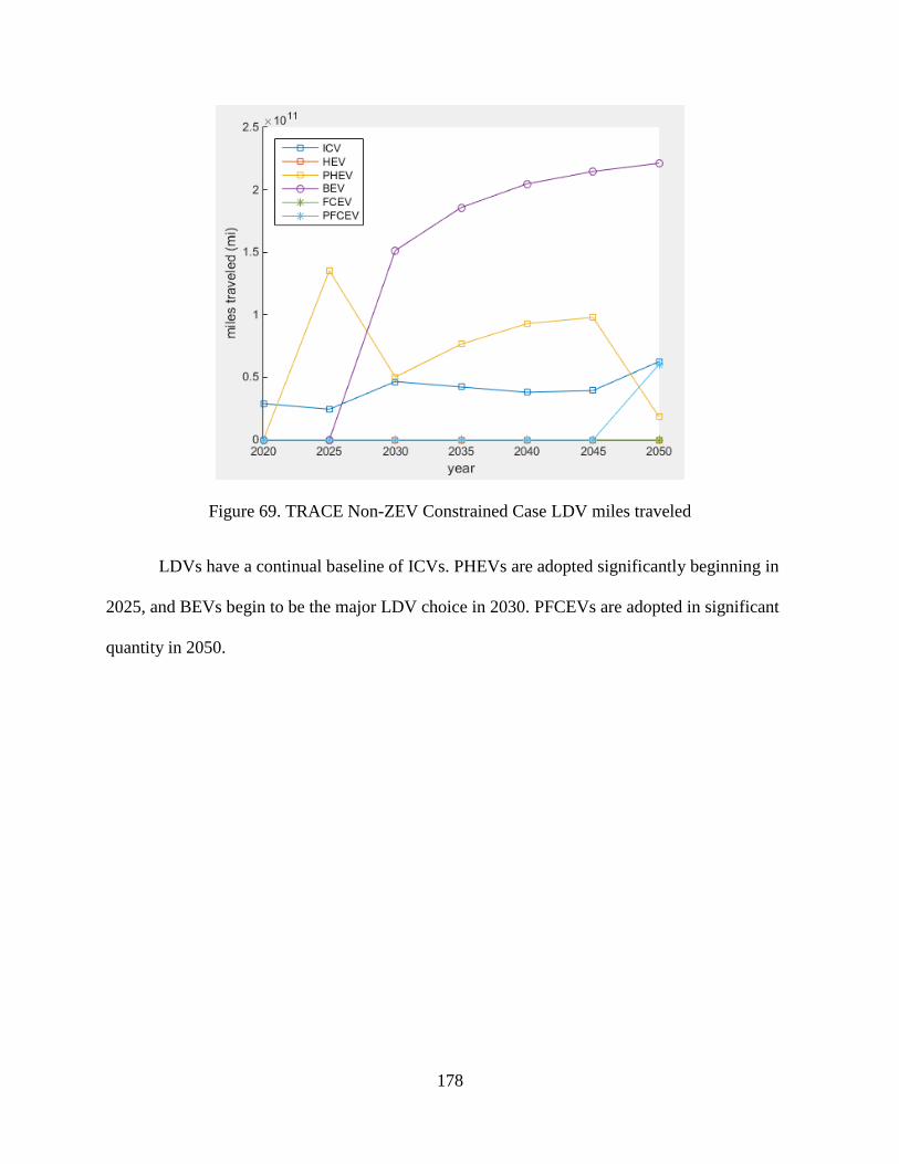
178

Figure 69. TRACE Non-ZEV Constrained Case LDV miles traveled

LDVs have a continual baseline of ICVs. PHEVs are adopted significantly beginning in

2025, and BEVs begin to be the major LDV choice in 2030. PFCEVs are adopted in significant

quantity in 2050.

179

Figure 70. TRACE Non-ZEV Constrained Case HDV miles traveled by vocation

HDVs of all vocations are composed solely of diesel-fueled ICVs up to and including in

2045. In 2050, diesel-fueled HEVs are the dominant or sole powertrain option for all vocations

except refuse. PFCEVs are also adopted for drayage trucks in somewhat significant quantities in

2050.

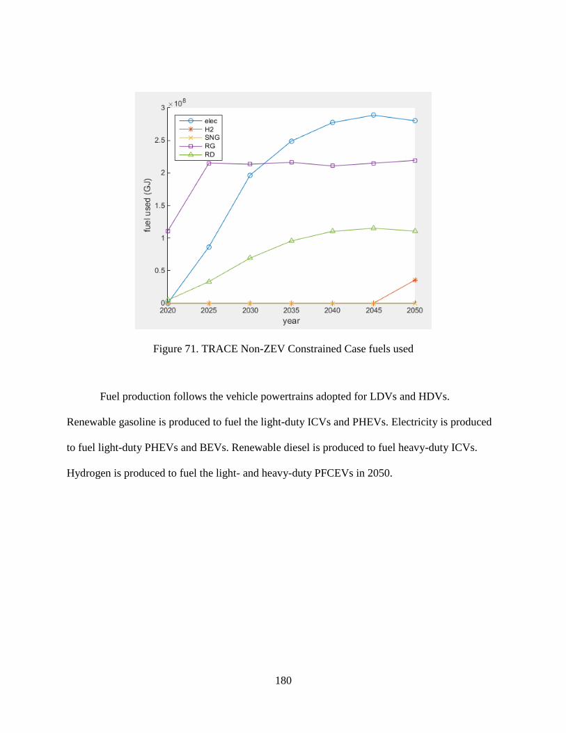
180

Figure 71. TRACE Non-ZEV Constrained Case fuels used

Fuel production follows the vehicle powertrains adopted for LDVs and HDVs.

Renewable gasoline is produced to fuel the light-duty ICVs and PHEVs. Electricity is produced

to fuel light-duty PHEVs and BEVs. Renewable diesel is produced to fuel heavy-duty ICVs.

Hydrogen is produced to fuel the light- and heavy-duty PFCEVs in 2050.

181

Figure 72. TRACE Non-ZEV Constrained Case feedstocks used

While waste begins as the most used fuel feedstock until 2030, electricity then becomes

the most used fuel feedstock as LDVs are primarily BEVs in later years and LDVs have

significantly higher VMT than HDVs. All biomass feedstock categories are used in various

quantities throughout the years of simulation.

Even though manure has a very negative GHG emission factor, it is not used much in

these results. This is because it is very expensive compared to waste, which is the most-used

biomass feedstock. Manure is about twice as expensive as the lowest cost waste on an energy

basis and 22% higher cost at waste’s highest cost (recall that many of the biomass feedstocks

have increasing cost as utilization increases). Therefore, TRACE finds another more cost-

effective fuel and vehicle pathway using waste to meet GHG emissions constraints.

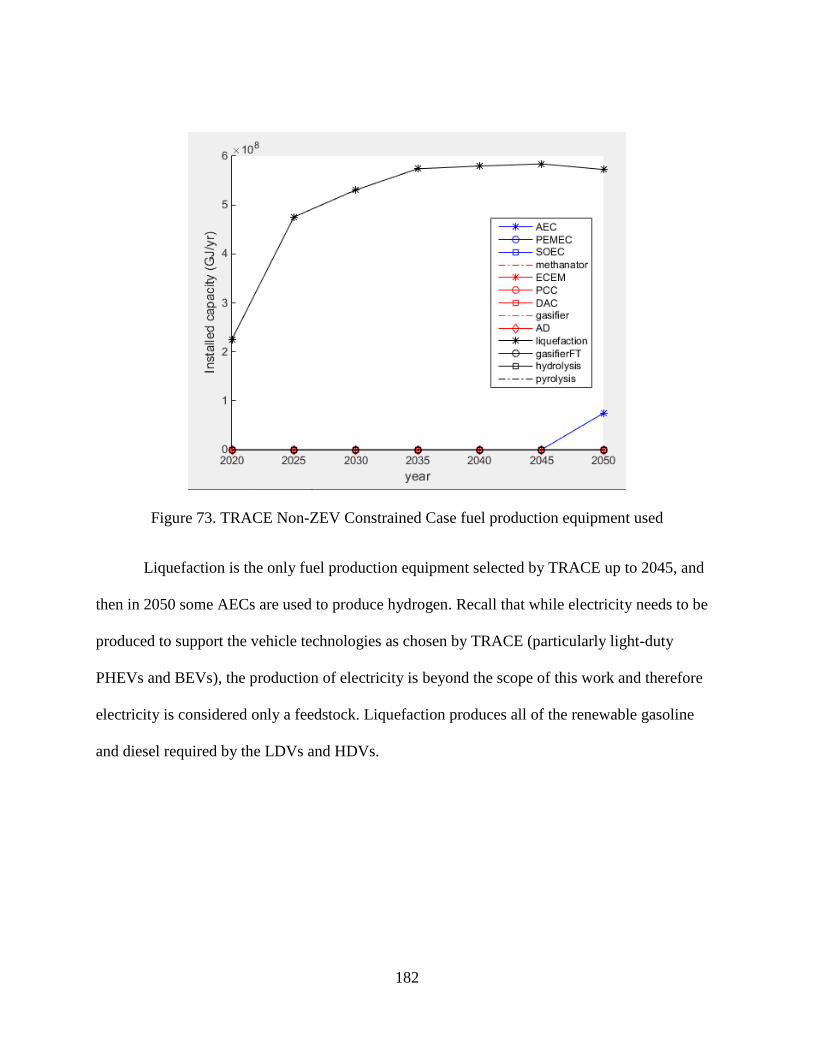
182

Figure 73. TRACE Non-ZEV Constrained Case fuel production equipment used

Liquefaction is the only fuel production equipment selected by TRACE up to 2045, and

then in 2050 some AECs are used to produce hydrogen. Recall that while electricity needs to be

produced to support the vehicle technologies as chosen by TRACE (particularly light-duty

PHEVs and BEVs), the production of electricity is beyond the scope of this work and therefore

electricity is considered only a feedstock. Liquefaction produces all of the renewable gasoline

and diesel required by the LDVs and HDVs.

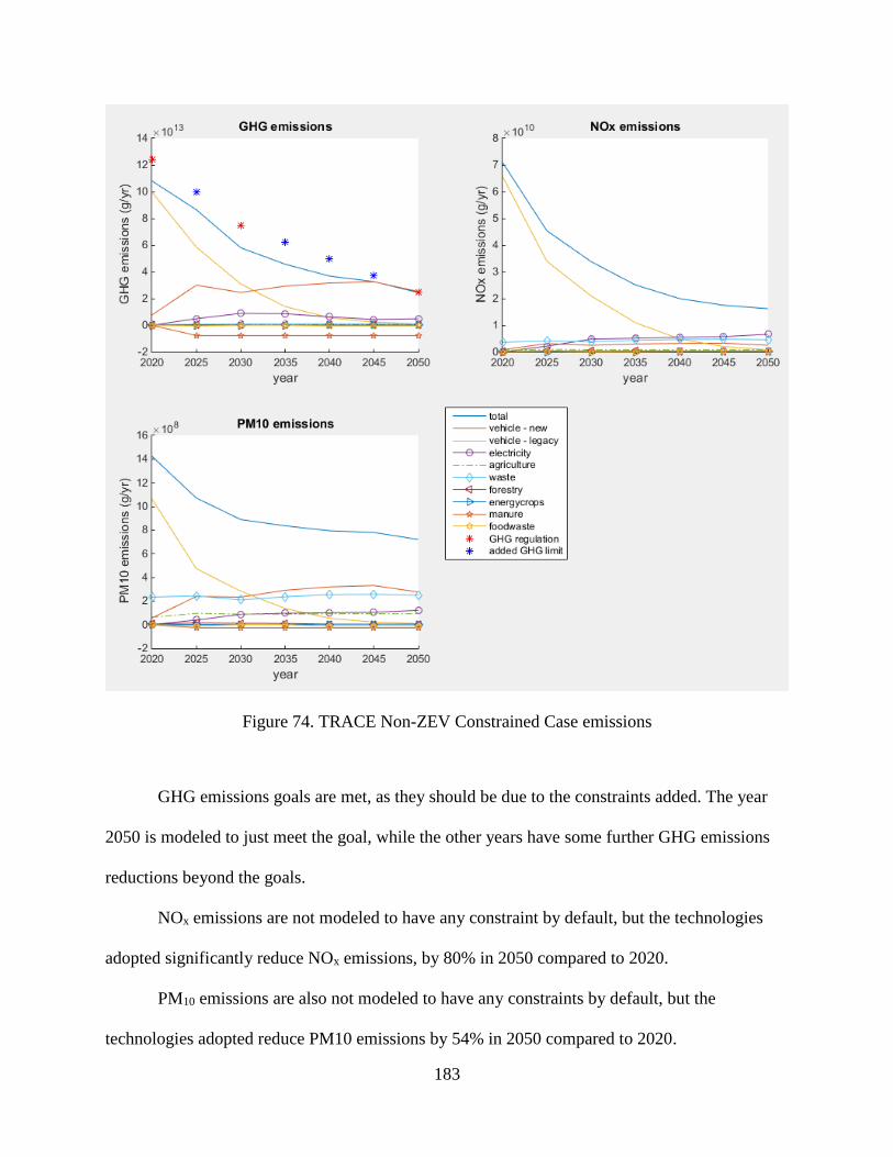
183

Figure 74. TRACE Non-ZEV Constrained Case emissions

GHG emissions goals are met, as they should be due to the constraints added. The year

2050 is modeled to just meet the goal, while the other years have some further GHG emissions

reductions beyond the goals.

NOx emissions are not modeled to have any constraint by default, but the technologies

adopted significantly reduce NOx emissions, by 80% in 2050 compared to 2020.

PM10 emissions are also not modeled to have any constraints by default, but the

technologies adopted reduce PM10 emissions by 54% in 2050 compared to 2020.

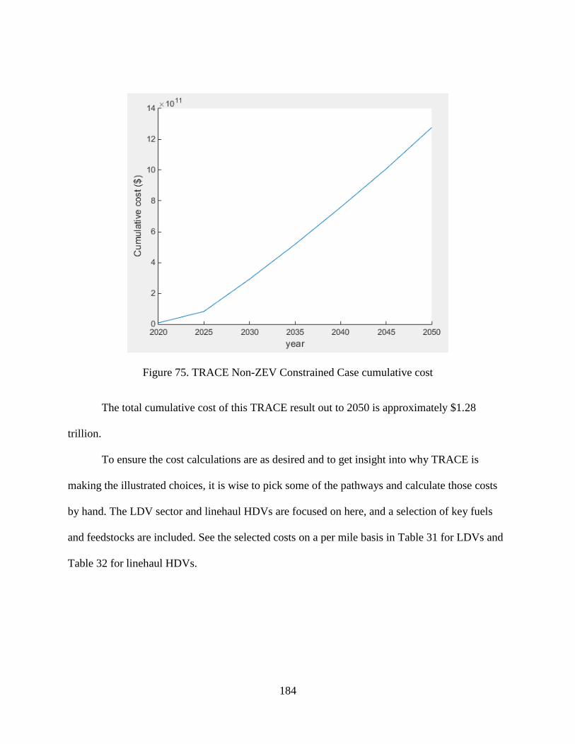
184

Figure 75. TRACE Non-ZEV Constrained Case cumulative cost

The total cumulative cost of this TRACE result out to 2050 is approximately $1.28

trillion.

To ensure the cost calculations are as desired and to get insight into why TRACE is

making the illustrated choices, it is wise to pick some of the pathways and calculate those costs

by hand. The LDV sector and linehaul HDVs are focused on here, and a selection of key fuels

and feedstocks are included. See the selected costs on a per mile basis in Table 31 for LDVs and

Table 32 for linehaul HDVs.

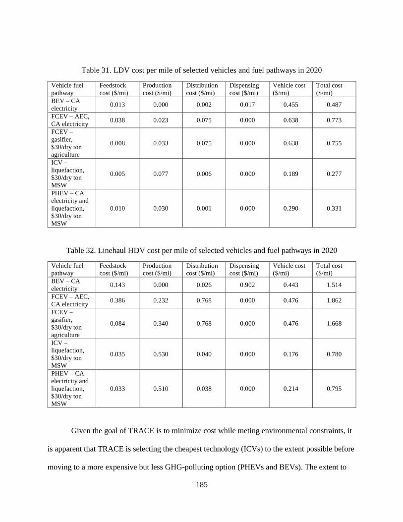
185

Table 31. LDV cost per mile of selected vehicles and fuel pathways in 2020

Vehicle fuel

pathway

Feedstock

cost ($/mi)

Production

cost ($/mi)

Distribution

cost ($/mi)

Dispensing

cost ($/mi)

Vehicle cost

($/mi)

Total cost

($/mi)

BEV – CA

electricity 0.013 0.000 0.002 0.017 0.455 0.487

FCEV – AEC,

CA electricity 0.038 0.023 0.075 0.000 0.638 0.773

FCEV –

gasifier,

$30/dry ton

agriculture

0.008 0.033 0.075 0.000 0.638 0.755

ICV –

liquefaction,

$30/dry ton

MSW

0.005 0.077 0.006 0.000 0.189 0.277

PHEV – CA

electricity and

liquefaction,

$30/dry ton

MSW

0.010 0.030 0.001 0.000 0.290 0.331

Table 32. Linehaul HDV cost per mile of selected vehicles and fuel pathways in 2020

Vehicle fuel

pathway

Feedstock

cost ($/mi)

Production

cost ($/mi)

Distribution

cost ($/mi)

Dispensing

cost ($/mi)

Vehicle cost

($/mi)

Total cost

($/mi)

BEV – CA

electricity 0.143 0.000 0.026 0.902 0.443 1.514

FCEV – AEC,

CA electricity 0.386 0.232 0.768 0.000 0.476 1.862

FCEV –

gasifier,

$30/dry ton

agriculture

0.084 0.340 0.768 0.000 0.476 1.668

ICV –

liquefaction,

$30/dry ton

MSW

0.035 0.530 0.040 0.000 0.176 0.780

PHEV – CA

electricity and

liquefaction,

$30/dry ton

MSW

0.033 0.510 0.038 0.000 0.214 0.795

Given the goal of TRACE is to minimize cost while meting environmental constraints, it

is apparent that TRACE is selecting the cheapest technology (ICVs) to the extent possible before

moving to a more expensive but less GHG-polluting option (PHEVs and BEVs). The extent to

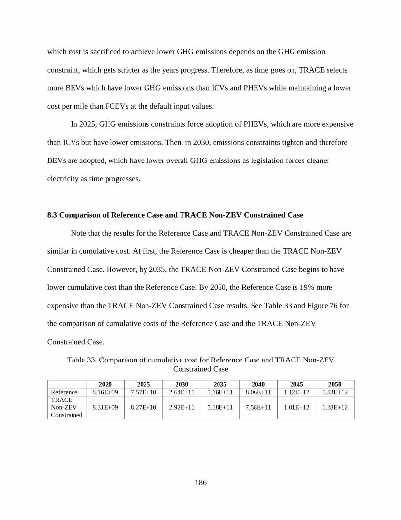
186

which cost is sacrificed to achieve lower GHG emissions depends on the GHG emission

constraint, which gets stricter as the years progress. Therefore, as time goes on, TRACE selects

more BEVs which have lower GHG emissions than ICVs and PHEVs while maintaining a lower

cost per mile than FCEVs at the default input values.

In 2025, GHG emissions constraints force adoption of PHEVs, which are more expensive

than ICVs but have lower emissions. Then, in 2030, emissions constraints tighten and therefore

BEVs are adopted, which have lower overall GHG emissions as legislation forces cleaner

electricity as time progresses.

8.3 Comparison of Reference Case and TRACE Non-ZEV Constrained Case

Note that the results for the Reference Case and TRACE Non-ZEV Constrained Case are

similar in cumulative cost. At first, the Reference Case is cheaper than the TRACE Non-ZEV

Constrained Case. However, by 2035, the TRACE Non-ZEV Constrained Case begins to have

lower cumulative cost than the Reference Case. By 2050, the Reference Case is 19% more

expensive than the TRACE Non-ZEV Constrained Case results. See Table 33 and Figure 76 for

the comparison of cumulative costs of the Reference Case and the TRACE Non-ZEV

Constrained Case.

Table 33. Comparison of cumulative cost for Reference Case and TRACE Non-ZEV

Constrained Case

2020 2025 2030 2035 2040 2045 2050

Reference 8.16E+09 7.57E+10 2.64E+11 5.16E+11 8.06E+11 1.12E+12 1.43E+12

TRACE

Non-ZEV

Constrained

8.31E+09 8.27E+10 2.92E+11 5.18E+11 7.58E+11 1.01E+12 1.28E+12

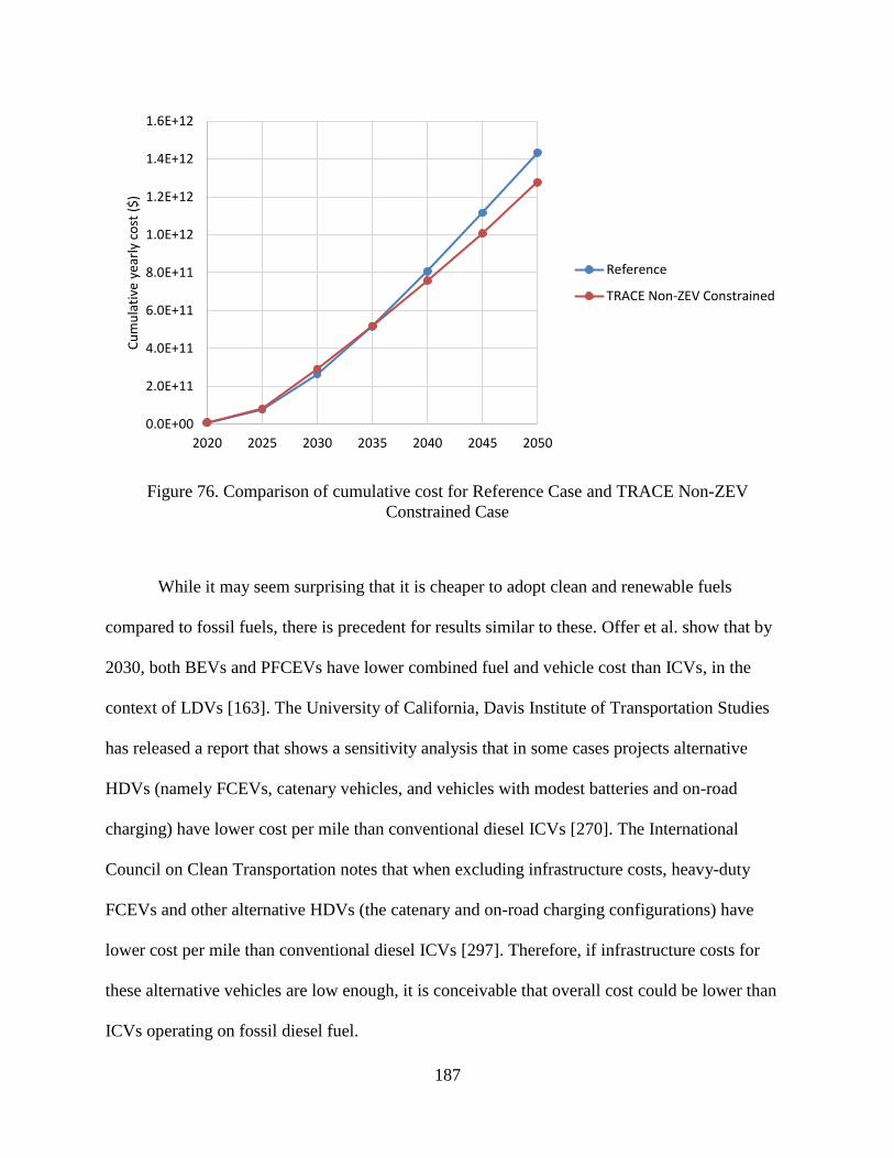
187

Figure 76. Comparison of cumulative cost for Reference Case and TRACE Non-ZEV

Constrained Case

While it may seem surprising that it is cheaper to adopt clean and renewable fuels

compared to fossil fuels, there is precedent for results similar to these. Offer et al. show that by

2030, both BEVs and PFCEVs have lower combined fuel and vehicle cost than ICVs, in the

context of LDVs [163]. The University of California, Davis Institute of Transportation Studies

has released a report that shows a sensitivity analysis that in some cases projects alternative

HDVs (namely FCEVs, catenary vehicles, and vehicles with modest batteries and on-road

charging) have lower cost per mile than conventional diesel ICVs [270]. The International

Council on Clean Transportation notes that when excluding infrastructure costs, heavy-duty

FCEVs and other alternative HDVs (the catenary and on-road charging configurations) have

lower cost per mile than conventional diesel ICVs [297]. Therefore, if infrastructure costs for

these alternative vehicles are low enough, it is conceivable that overall cost could be lower than

ICVs operating on fossil diesel fuel.

0.0E+00

2.0E+11

4.0E+11

6.0E+11

8.0E+11

1.0E+12

1.2E+12

1.4E+12

1.6E+12

2020 2025 2030 2035 2040 2045 2050

Cu

mu

lati

ve y

earl

y co

st (

$)

Reference

TRACE Non-ZEV Constrained

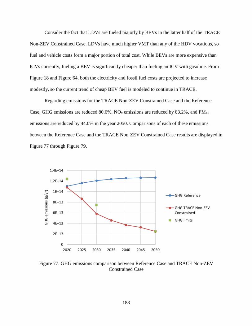
188

Consider the fact that LDVs are fueled majorly by BEVs in the latter half of the TRACE

Non-ZEV Constrained Case. LDVs have much higher VMT than any of the HDV vocations, so

fuel and vehicle costs form a major portion of total cost. While BEVs are more expensive than

ICVs currently, fueling a BEV is significantly cheaper than fueling an ICV with gasoline. From

Figure 18 and Figure 64, both the electricity and fossil fuel costs are projected to increase

modestly, so the current trend of cheap BEV fuel is modeled to continue in TRACE.

Regarding emissions for the TRACE Non-ZEV Constrained Case and the Reference

Case, GHG emissions are reduced 80.6%, NOx emissions are reduced by 83.2%, and PM10

emissions are reduced by 44.0% in the year 2050. Comparisons of each of these emissions

between the Reference Case and the TRACE Non-ZEV Constrained Case results are displayed in

Figure 77 through Figure 79.

Figure 77. GHG emissions comparison between Reference Case and TRACE Non-ZEV

Constrained Case

0

2E+13

4E+13

6E+13

8E+13

1E+14

1.2E+14

1.4E+14

2020 2025 2030 2035 2040 2045 2050

GH

G e

mis

sio

ns

(g/y

r)

GHG Reference

GHG TRACE Non-ZEVConstrained

GHG limits

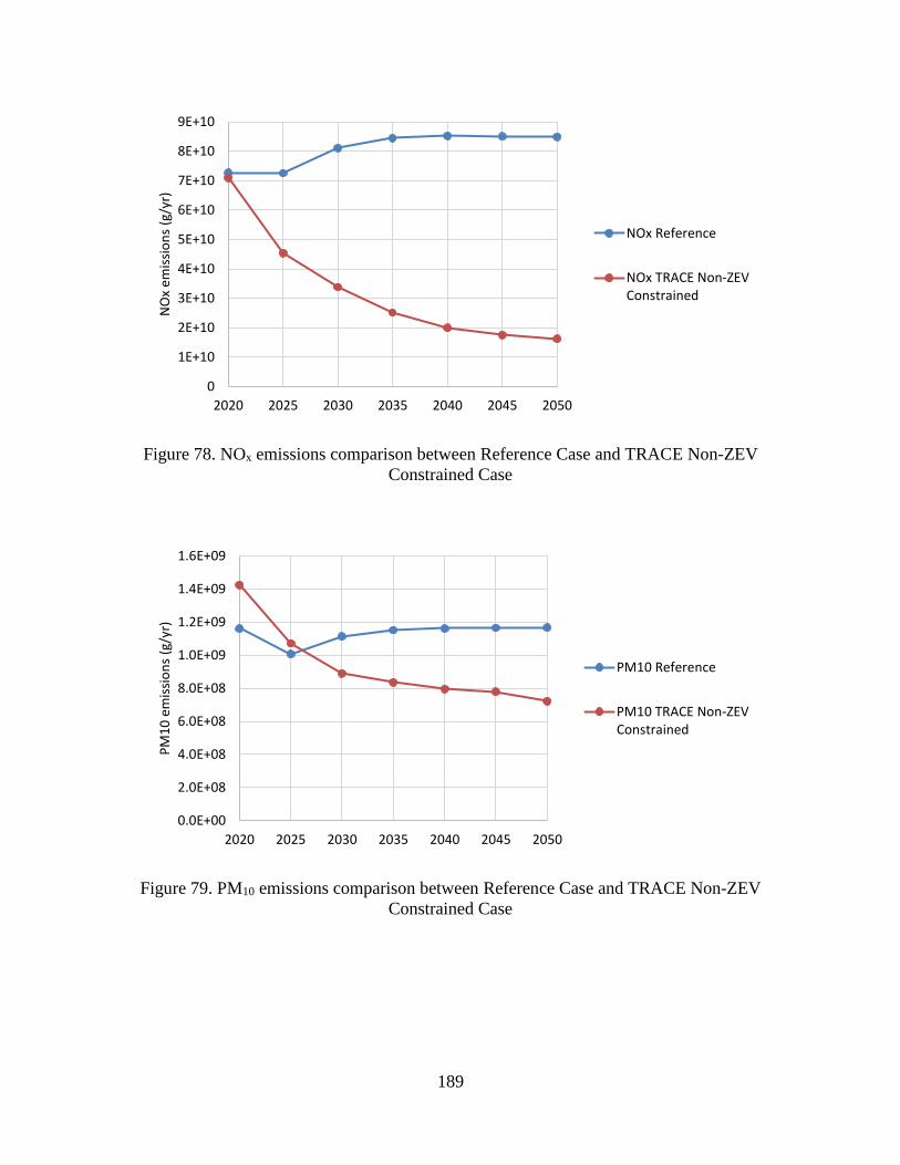
189

Figure 78. NOx emissions comparison between Reference Case and TRACE Non-ZEV

Constrained Case

Figure 79. PM10 emissions comparison between Reference Case and TRACE Non-ZEV

Constrained Case

0

1E+10

2E+10

3E+10

4E+10

5E+10

6E+10

7E+10

8E+10

9E+10

2020 2025 2030 2035 2040 2045 2050

NO

x em

issi

on

s (g

/yr)

NOx Reference

NOx TRACE Non-ZEVConstrained

0.0E+00

2.0E+08

4.0E+08

6.0E+08

8.0E+08

1.0E+09

1.2E+09

1.4E+09

1.6E+09

2020 2025 2030 2035 2040 2045 2050

PM

10

em

issi

on

s (g

/yr)

PM10 Reference

PM10 TRACE Non-ZEVConstrained

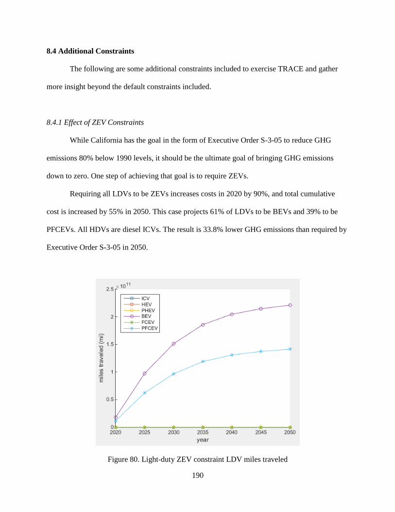
190

8.4 Additional Constraints

The following are some additional constraints included to exercise TRACE and gather

more insight beyond the default constraints included.

8.4.1 Effect of ZEV Constraints

While California has the goal in the form of Executive Order S-3-05 to reduce GHG

emissions 80% below 1990 levels, it should be the ultimate goal of bringing GHG emissions

down to zero. One step of achieving that goal is to require ZEVs.

Requiring all LDVs to be ZEVs increases costs in 2020 by 90%, and total cumulative

cost is increased by 55% in 2050. This case projects 61% of LDVs to be BEVs and 39% to be

PFCEVs. All HDVs are diesel ICVs. The result is 33.8% lower GHG emissions than required by

Executive Order S-3-05 in 2050.

Figure 80. Light-duty ZEV constraint LDV miles traveled

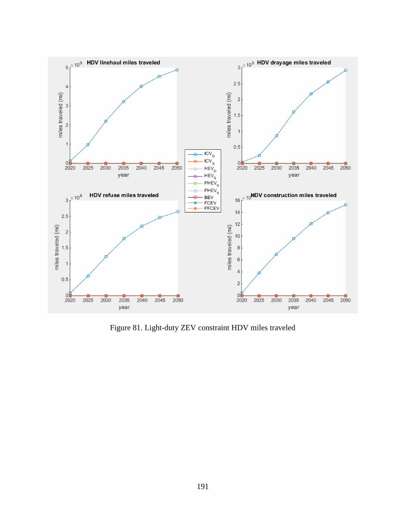
191

Figure 81. Light-duty ZEV constraint HDV miles traveled

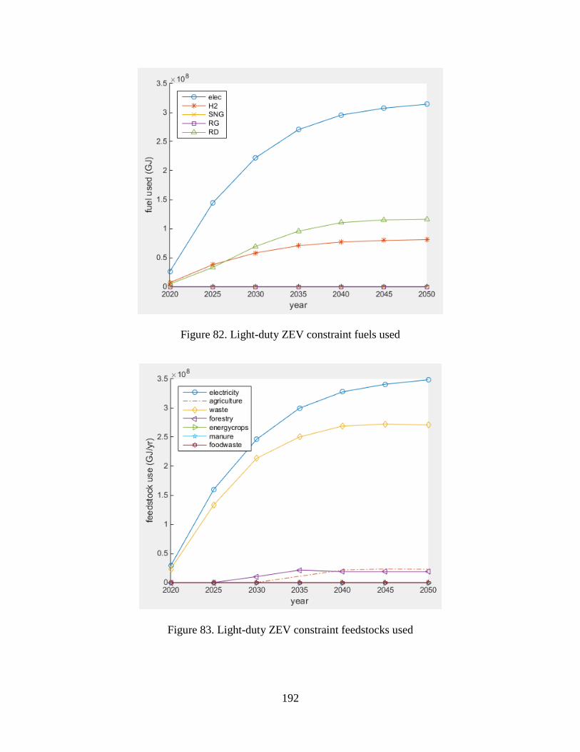
192

Figure 82. Light-duty ZEV constraint fuels used

Figure 83. Light-duty ZEV constraint feedstocks used

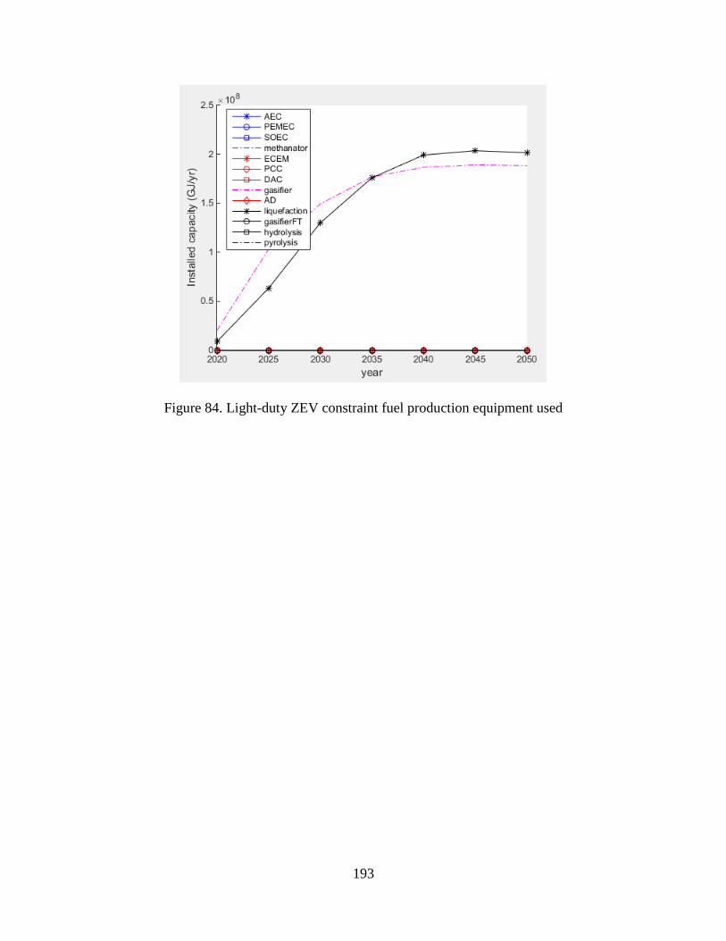
193

Figure 84. Light-duty ZEV constraint fuel production equipment used

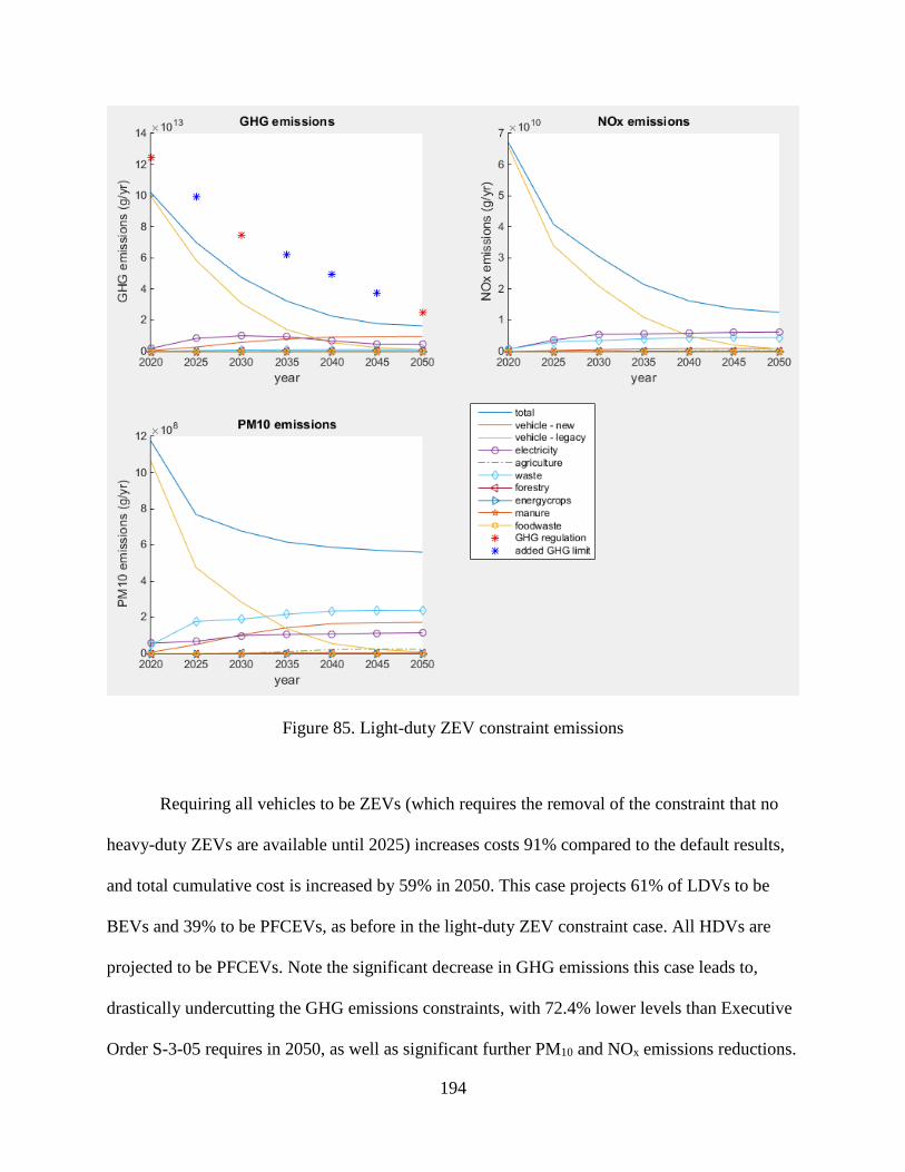
194

Figure 85. Light-duty ZEV constraint emissions

Requiring all vehicles to be ZEVs (which requires the removal of the constraint that no

heavy-duty ZEVs are available until 2025) increases costs 91% compared to the default results,

and total cumulative cost is increased by 59% in 2050. This case projects 61% of LDVs to be

BEVs and 39% to be PFCEVs, as before in the light-duty ZEV constraint case. All HDVs are

projected to be PFCEVs. Note the significant decrease in GHG emissions this case leads to,

drastically undercutting the GHG emissions constraints, with 72.4% lower levels than Executive

Order S-3-05 requires in 2050, as well as significant further PM10 and NOx emissions reductions.

195

Figure 86. All ZEV constraint fuels used

Figure 87. All ZEV constraint fuel feedstocks used

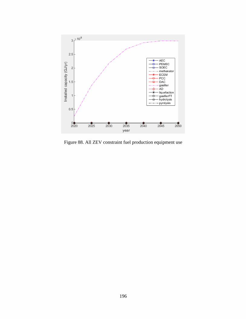
196

Figure 88. All ZEV constraint fuel production equipment use

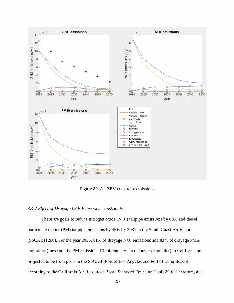
197

Figure 89. All ZEV constraint emissions

8.4.2 Effect of Drayage CAP Emissions Constraints

There are goals to reduce nitrogen oxide (NOx) tailpipe emissions by 80% and diesel

particulate matter (PM) tailpipe emissions by 45% by 2031 in the South Coast Air Basin

(SoCAB) [298]. For the year 2035, 81% of drayage NOx emissions and 82% of drayage PM10

emissions (these are the PM emissions 10 micrometers in diameter or smaller) in California are

projected to be from ports in the SoCAB (Port of Los Angeles and Port of Long Beach)

according to the California Air Resources Board Standard Emission Tool [299]. Therefore, due

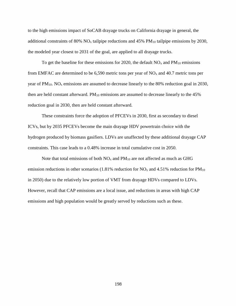
198

to the high emissions impact of SoCAB drayage trucks on California drayage in general, the

additional constraints of 80% NOx tailpipe reductions and 45% PM10 tailpipe emissions by 2030,

the modeled year closest to 2031 of the goal, are applied to all drayage trucks.

To get the baseline for these emissions for 2020, the default NOx and PM10 emissions

from EMFAC are determined to be 6,590 metric tons per year of NOx and 40.7 metric tons per

year of PM10. NOx emissions are assumed to decrease linearly to the 80% reduction goal in 2030,

then are held constant afterward. PM10 emissions are assumed to decrease linearly to the 45%

reduction goal in 2030, then are held constant afterward.

These constraints force the adoption of PFCEVs in 2030, first as secondary to diesel

ICVs, but by 2035 PFCEVs become the main drayage HDV powertrain choice with the

hydrogen produced by biomass gasifiers. LDVs are unaffected by these additional drayage CAP

constraints. This case leads to a 0.48% increase in total cumulative cost in 2050.

Note that total emissions of both NOx and PM10 are not affected as much as GHG

emission reductions in other scenarios (1.81% reduction for NOx and 4.51% reduction for PM10

in 2050) due to the relatively low portion of VMT from drayage HDVs compared to LDVs.

However, recall that CAP emissions are a local issue, and reductions in areas with high CAP

emissions and high population would be greatly served by reductions such as these.

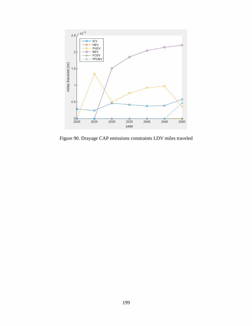
199

Figure 90. Drayage CAP emissions constraints LDV miles traveled

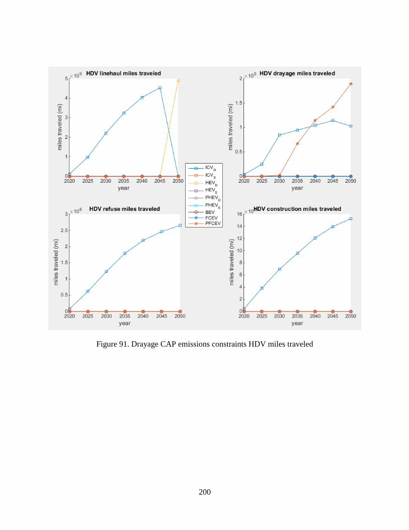
200

Figure 91. Drayage CAP emissions constraints HDV miles traveled

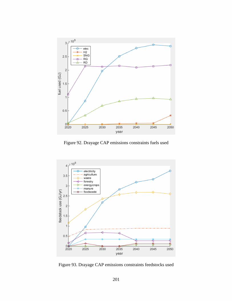
201

Figure 92. Drayage CAP emissions constraints fuels used

Figure 93. Drayage CAP emissions constraints feedstocks used

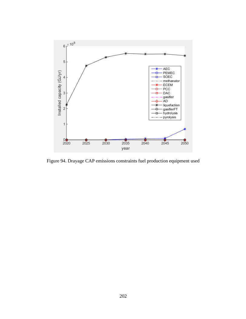
202

Figure 94. Drayage CAP emissions constraints fuel production equipment used

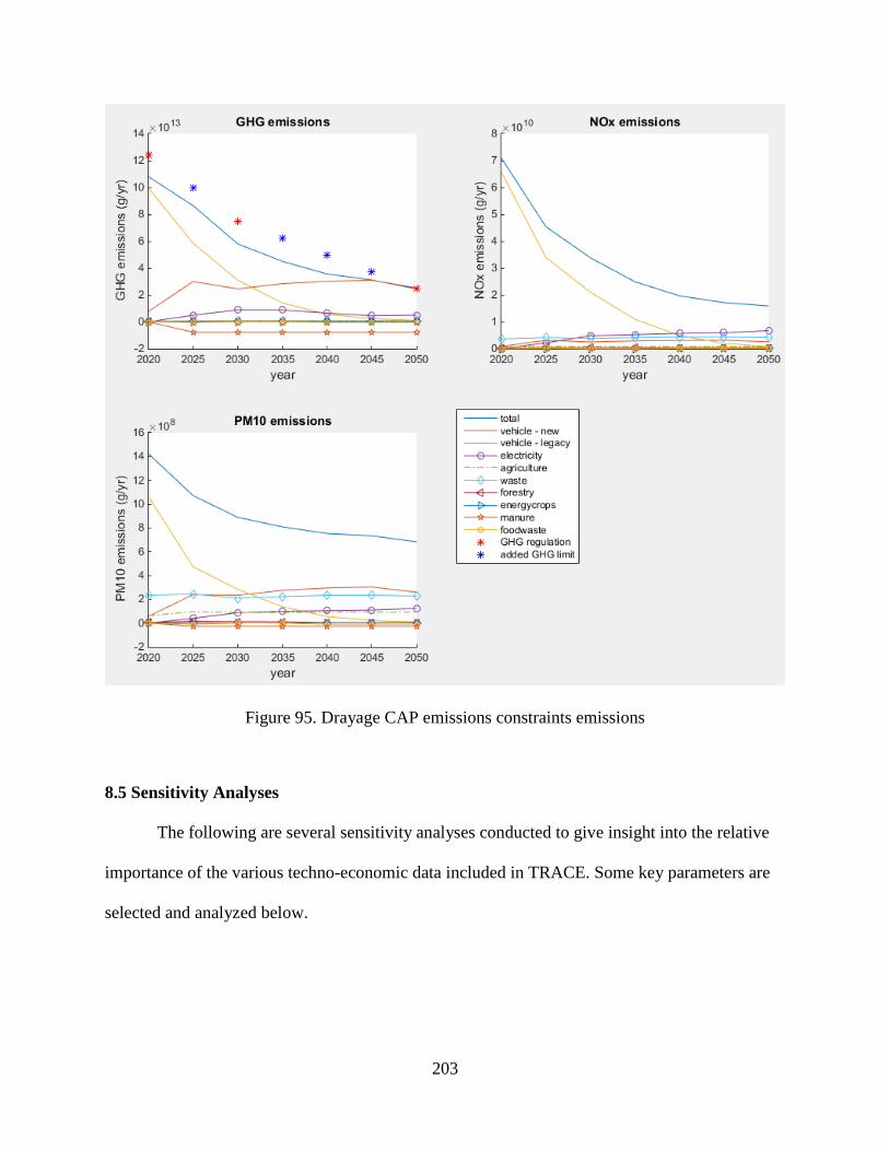
203

Figure 95. Drayage CAP emissions constraints emissions

8.5 Sensitivity Analyses

The following are several sensitivity analyses conducted to give insight into the relative

importance of the various techno-economic data included in TRACE. Some key parameters are

selected and analyzed below.

204

8.5.1 Effect of Continued Production Plant Constraint

The use of CRFs to convert the capital cost of fuel production plants requires the

constraint that when a production technology is adopted, it will continue to be used and paid for

until the end of its lifetime (or the end of this analysis in 2050, after which is beyond the scope of

this work). However, it would be interesting to see the effect of removing that constraint,

effectively making the fuel production market infinitely flexible to respond to change in cost of

fuel and vehicle pathways. Doing so causes a drastic decrease in liquefaction production plant

use in 2050.

Figure 96. No continued production plant constraint LDV miles traveled

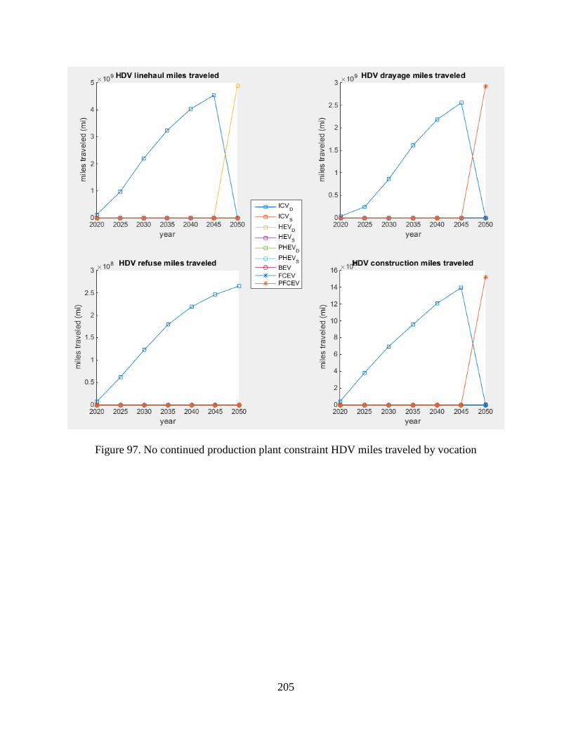
205

Figure 97. No continued production plant constraint HDV miles traveled by vocation

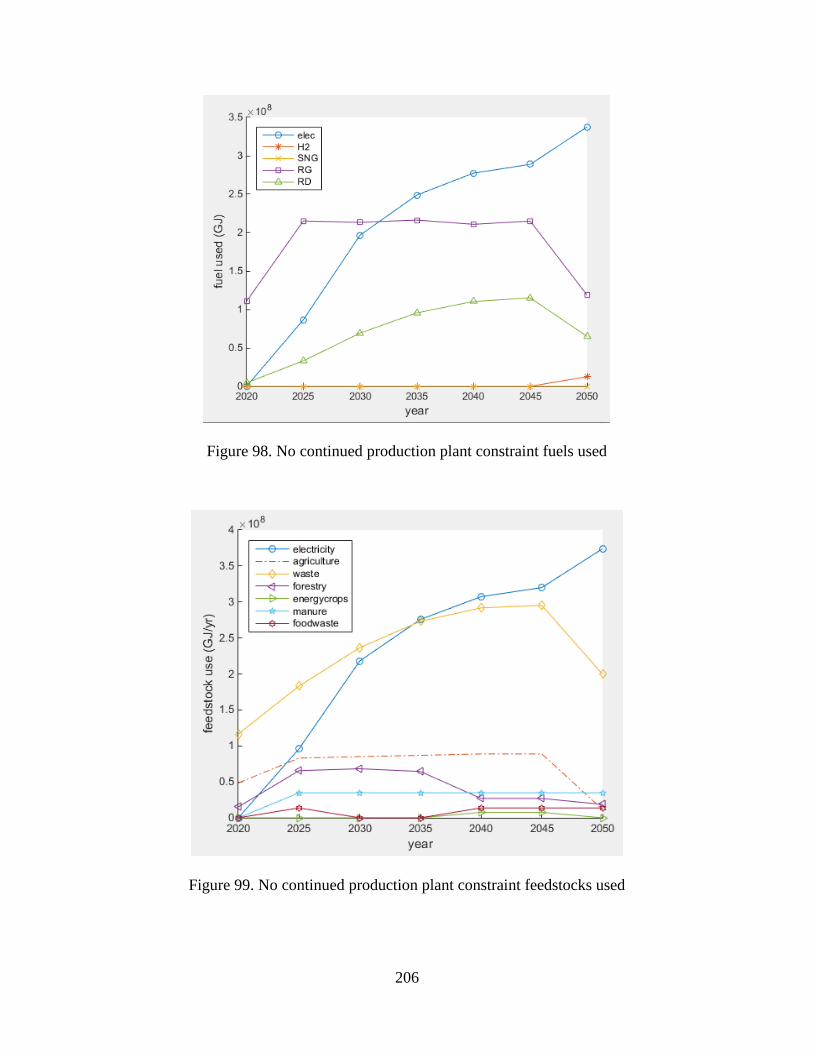
206

Figure 98. No continued production plant constraint fuels used

Figure 99. No continued production plant constraint feedstocks used

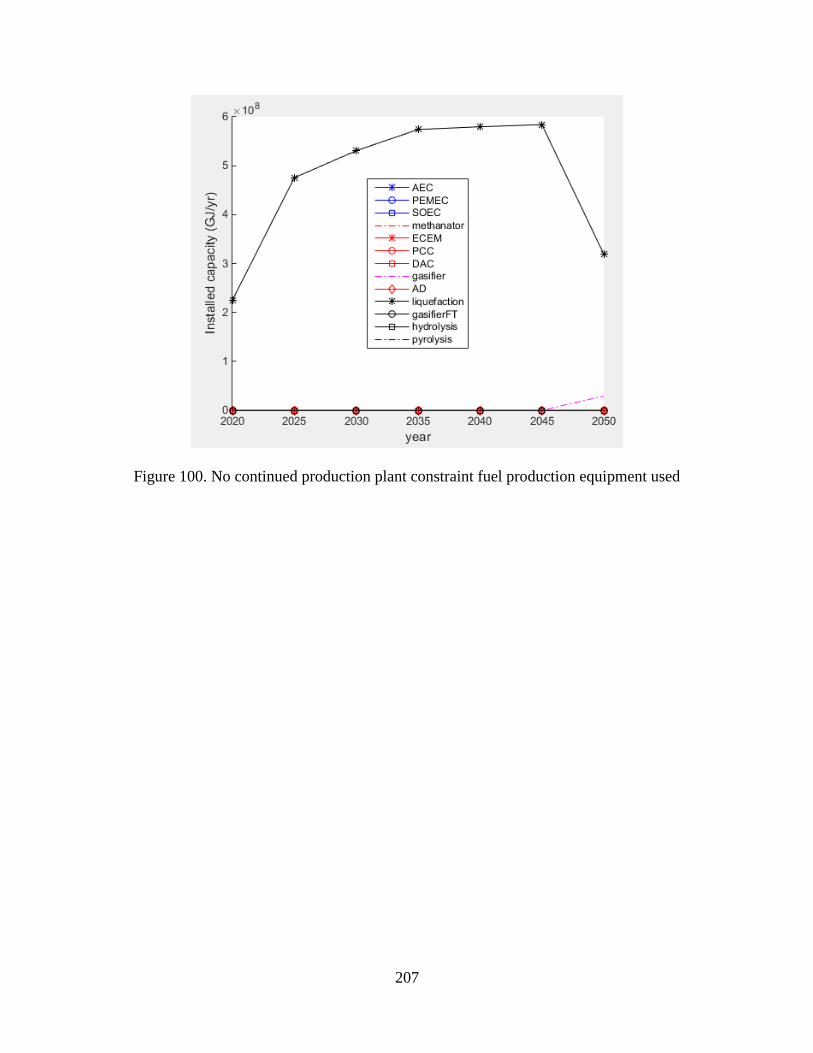
207

Figure 100. No continued production plant constraint fuel production equipment used

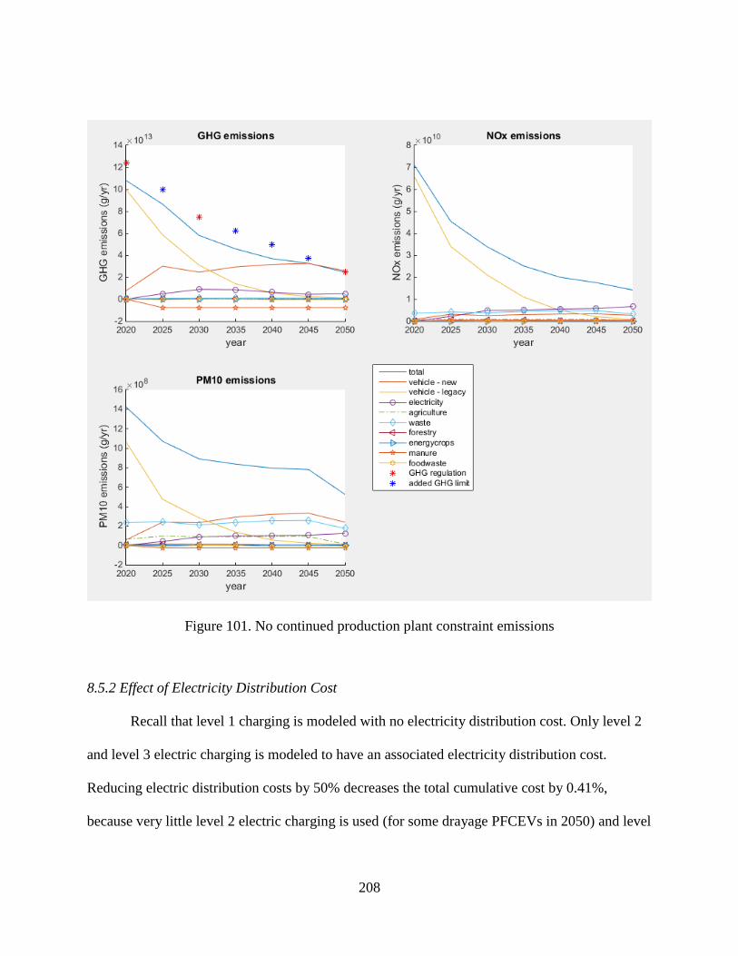
208

Figure 101. No continued production plant constraint emissions

8.5.2 Effect of Electricity Distribution Cost

Recall that level 1 charging is modeled with no electricity distribution cost. Only level 2

and level 3 electric charging is modeled to have an associated electricity distribution cost.

Reducing electric distribution costs by 50% decreases the total cumulative cost by 0.41%,

because very little level 2 electric charging is used (for some drayage PFCEVs in 2050) and level

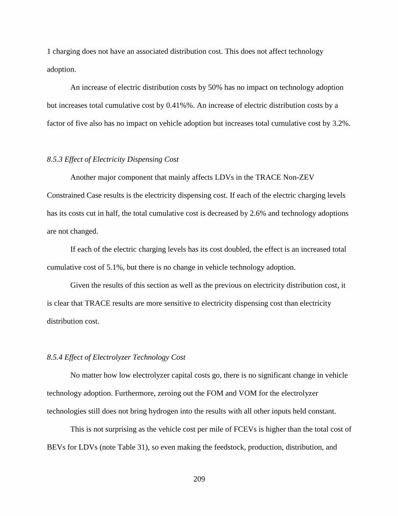
209

1 charging does not have an associated distribution cost. This does not affect technology

adoption.

An increase of electric distribution costs by 50% has no impact on technology adoption

but increases total cumulative cost by 0.41%%. An increase of electric distribution costs by a

factor of five also has no impact on vehicle adoption but increases total cumulative cost by 3.2%.

8.5.3 Effect of Electricity Dispensing Cost

Another major component that mainly affects LDVs in the TRACE Non-ZEV

Constrained Case results is the electricity dispensing cost. If each of the electric charging levels

has its costs cut in half, the total cumulative cost is decreased by 2.6% and technology adoptions

are not changed.

If each of the electric charging levels has its cost doubled, the effect is an increased total

cumulative cost of 5.1%, but there is no change in vehicle technology adoption.

Given the results of this section as well as the previous on electricity distribution cost, it

is clear that TRACE results are more sensitive to electricity dispensing cost than electricity

distribution cost.

8.5.4 Effect of Electrolyzer Technology Cost

No matter how low electrolyzer capital costs go, there is no significant change in vehicle

technology adoption. Furthermore, zeroing out the FOM and VOM for the electrolyzer

technologies still does not bring hydrogen into the results with all other inputs held constant.

This is not surprising as the vehicle cost per mile of FCEVs is higher than the total cost of

BEVs for LDVs (note Table 31), so even making the feedstock, production, distribution, and

210

dispensing costs all zero for hydrogen pathways would not be enough to stimulate an adoption of

fuel cell-powered vehicles beyond that required to make up for range and fueling time

constraints of BEVs.

8.5.5 Effect of Gasifier Cost

Similar to the electrolyzer costs, zeroing out gasifier capital, FOM, and VOM costs still is

not enough to get hydrogen adopted and results are the same as default. The same reason as

above regarding high FCEV cost is relevant here.

8.5.6 Effect of Fuel Cell Cost

Reducing fuel cell cost to $0 does not encourage the adoption of either FCEVs or

PFCEVs beyond what is adopted in the Non-ZEV Constrained Case.

8.5.7 Effect of Liquefaction Cost

Reducing the starting liquefaction cost 10% lowers the total cumulative cost by 0.55%

and does not change technology adoption. Increasing the starting liquefaction cost by 10%

increases the total cumulative cost by 0.54% and also does not change technology adoption.

Doubling liquefaction capital costs leads to a total cumulative cost reduction of 2.9% due

to technologies adopted. This causes LDVs to be primarily PHEVs and BEVs beginning in 2025,

while HDV vocations assume several alternative powertrain options except for refuse trucks.

PHEVs to be adopted in 2020 instead of ICVs. The amount of liquefaction adopted is

significantly decreased and electricity use is correspondingly increased.

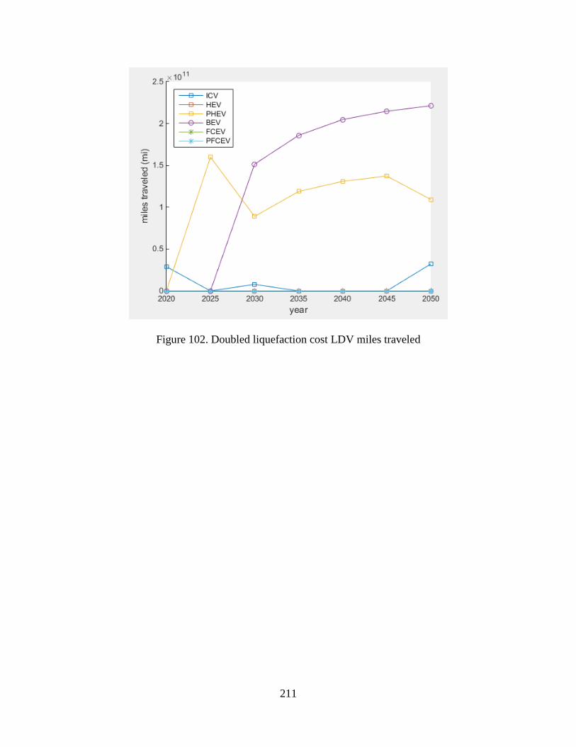
211

Figure 102. Doubled liquefaction cost LDV miles traveled

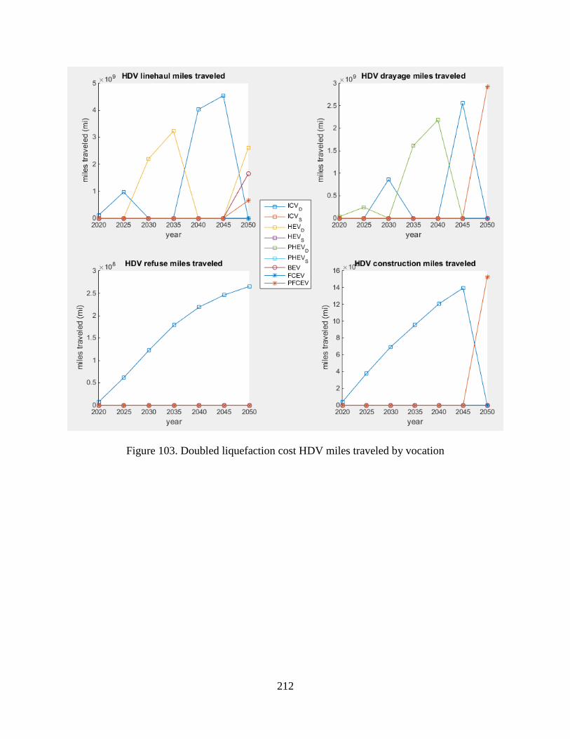
212

Figure 103. Doubled liquefaction cost HDV miles traveled by vocation

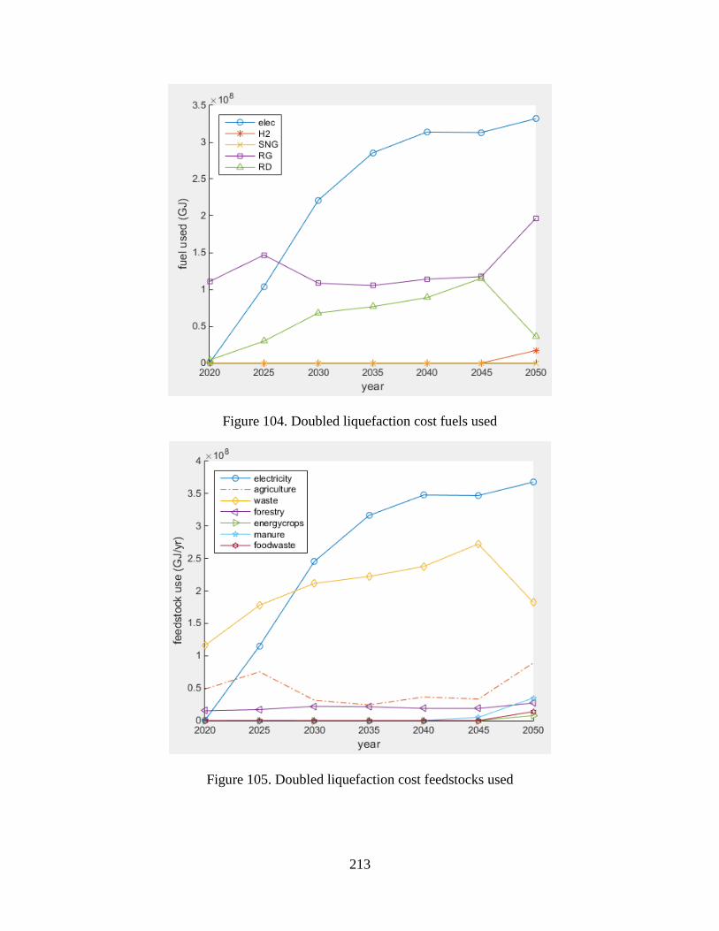
213

Figure 104. Doubled liquefaction cost fuels used

Figure 105. Doubled liquefaction cost feedstocks used

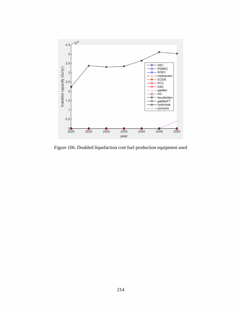
214

Figure 106. Doubled liquefaction cost fuel production equipment used

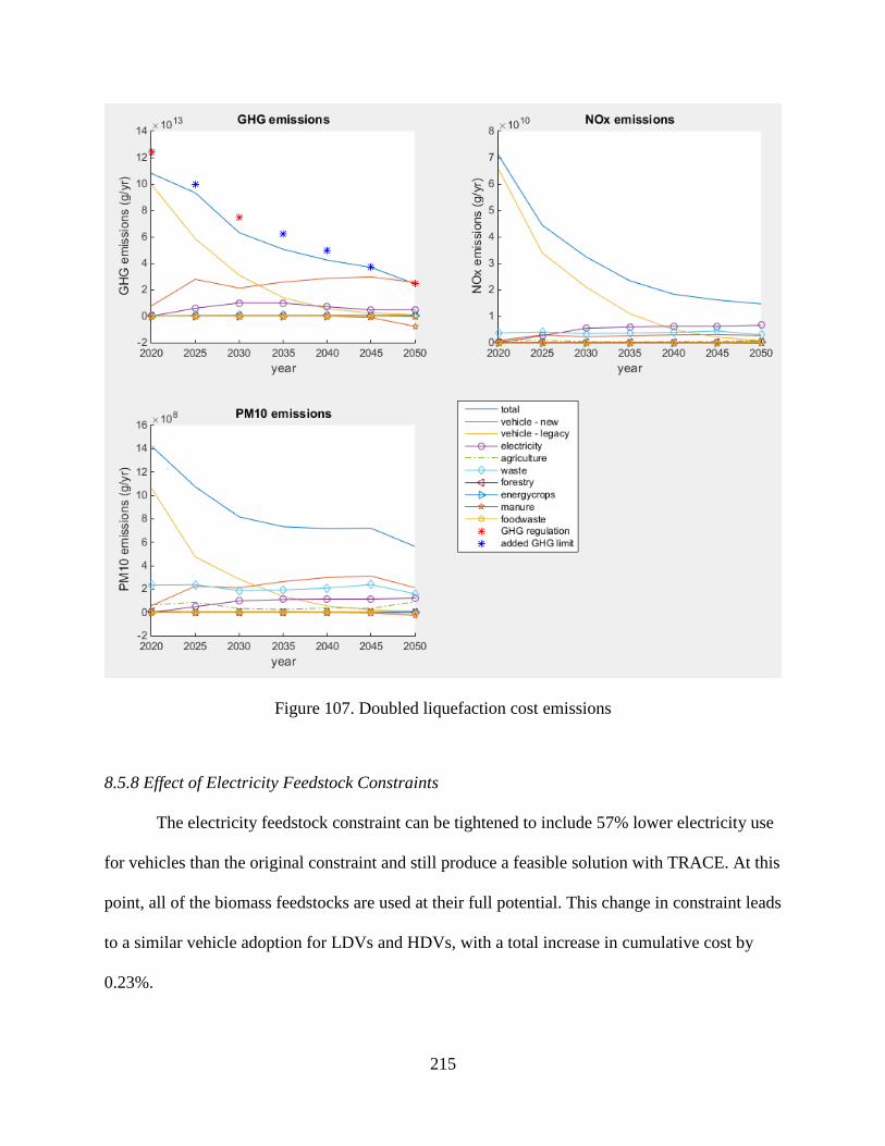
215

Figure 107. Doubled liquefaction cost emissions

8.5.8 Effect of Electricity Feedstock Constraints

The electricity feedstock constraint can be tightened to include 57% lower electricity use

for vehicles than the original constraint and still produce a feasible solution with TRACE. At this

point, all of the biomass feedstocks are used at their full potential. This change in constraint leads

to a similar vehicle adoption for LDVs and HDVs, with a total increase in cumulative cost by

0.23%.

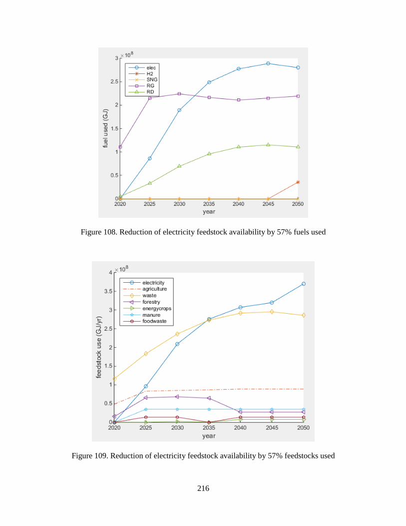
216

Figure 108. Reduction of electricity feedstock availability by 57% fuels used

Figure 109. Reduction of electricity feedstock availability by 57% feedstocks used

217

8.5.9 Effect of CF and Electricity Cost on P2G Technology

Electricity costs from E3 are somewhat low [300], ranging from 3.7 cents per kWh in

2020 to 4.2 cents per kWh in 2050 with some fluctuation in the middle [189]. Consider a case

with a 50% increase in the electricity cost for BEVs, which is more conservative, and negligible

cost for electricity going into P2G plants, a scenario that could exist given the already existing

curtailed energy from solar and wind power in California [301][302]. However, if a P2G plant is

using otherwise-curtailed electricity, the capacity factor would be low; assume a capacity factor

of 0.2 instead of the default 0.8. With these changes in electricity cost and P2G plant capacity

factor, the technology adoption stays the same as for the default electricity costs. Total

cumulative cost increases 2.5% due to the heavy light-duty BEV use and the 50% increase of

fuel cost for those vehicles.

8.5.10 Effect of Battery Learning Rate

Decreasing the battery learning rate to zero, meaning there is no decrease in battery cost

with increasing cumulative production amount, has a number of impacts on technology adoption.

For LDVs, PHEVs are used into later years of modeling and PFCEVs are adopted as the primary

powertrain type in 2045 and 2050. Linehaul HDVs have significant diesel HEV adoption in 2030

and some significant PFCEV adoption in 2035 and 2040, respectively. Drayage HDVs have

significant PFCEV adoption in 2030 and beyond, except in 2040. Refuse HDVs continue to use

diesel ICVs. For construction HDVs, there is some significant PFCEV and FCEV adoption in

2030 and 2040, respectively. Total cumulative cost is increased 22%, showing battery cost is a

major contributor to total cost of these TRACE results.

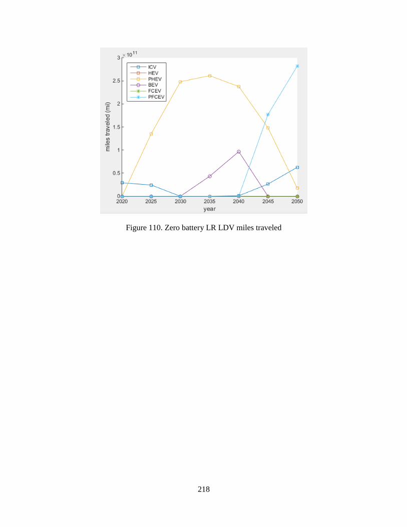
218

Figure 110. Zero battery LR LDV miles traveled

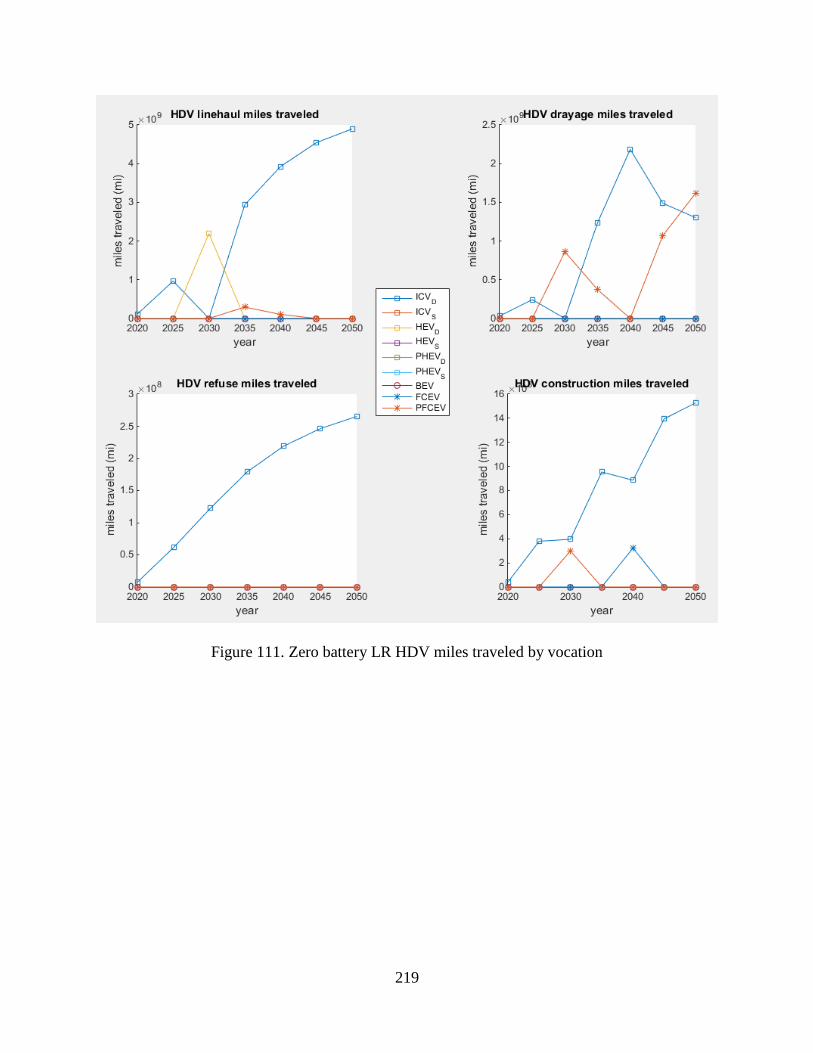
219

Figure 111. Zero battery LR HDV miles traveled by vocation

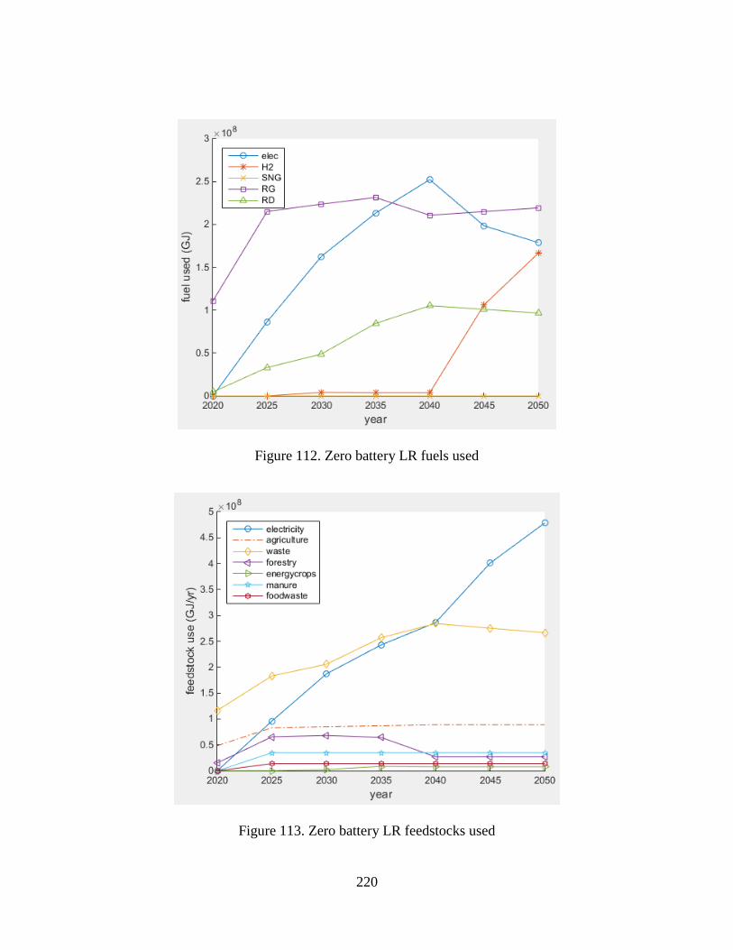
220

Figure 112. Zero battery LR fuels used

Figure 113. Zero battery LR feedstocks used

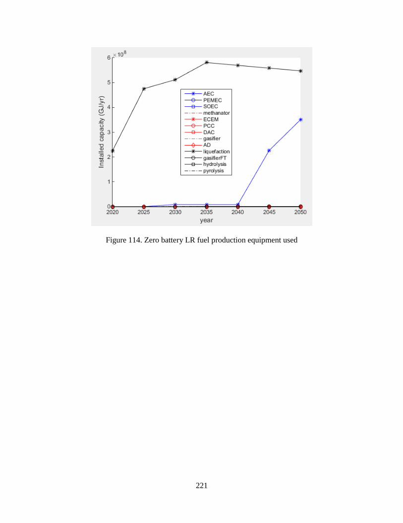
221

Figure 114. Zero battery LR fuel production equipment used

222

Figure 115. Zero battery LR emissions

8.5.11 Effect of VMT Changes

As previously mentioned, VMT projections are from EMFAC [141]. As with all

projections, it would be unwise to assume that these projections are entirely accurate. This is

especially true as drastically increasing alternative fuel and vehicle use (as projected by TRACE

using default values) would affect cost of transportation, particularly in early years of adoption.

TRACE is perfectly inelastic to demand, meaning changes in cost do not affect demand (i.e.

VMT). Therefore, it is important to include a sensitivity analysis for VMT. Additionally, the

223

literature shows a range of VMT changes due to autonomous vehicles, with some projections up

to 100% increase of VMT [303]–[312]. While the changes in efficiency and cost of autonomous

vehicles compared to human-driven vehicles is beyond the scope of this work (and therefore no

changes are made to the efficiency or cost in the following cases), the potential change in VMT

is modeled so a general idea of the effect of varying VMT demand can be analyzed. Note that

only the VMT of the new vehicles using the alternative fuels is affected here, as the legacy

vehicles are assumed to use fossil fuels with consistent fuel price so VMT for those vehicles is

assumed constant.

Decreasing VMT has the potential to drastically change adopted technologies, depending

on the magnitude of increase in VMT. Decreasing VMT 10% for all years decreases cumulative

cost by 9.9%, but does not affect the rollout of fuel and vehicle technologies. Decreasing VMT

50% for all years decreases cumulative cost by 48% and does affect the rollout of fuel and

vehicle technologies. Due to significantly lower VMT, meeting emissions reductions goals does

not require as many alternative vehicle types. The result is more reliance on ICVs for both LDVs

and HDVs while still meeting the GHG emissions goals.

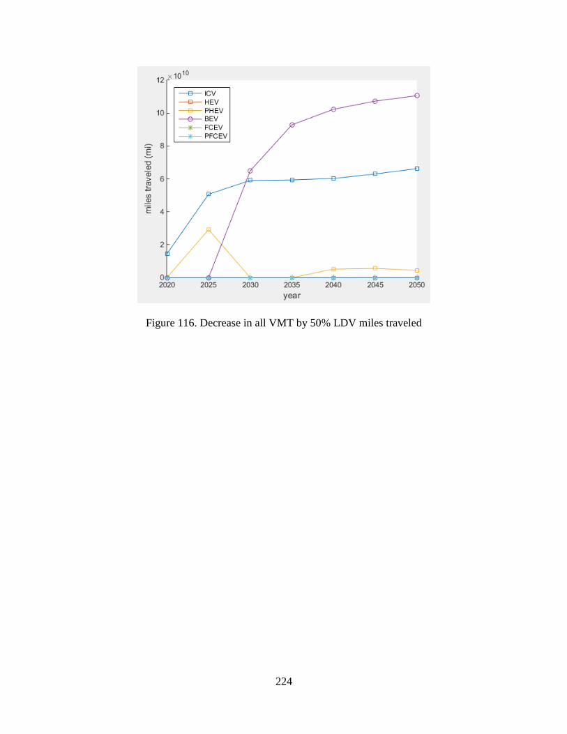
224

Figure 116. Decrease in all VMT by 50% LDV miles traveled

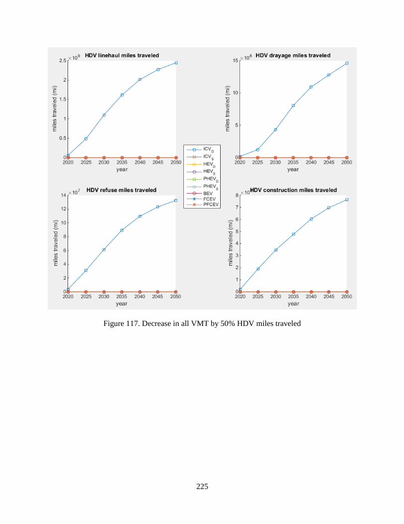
225

Figure 117. Decrease in all VMT by 50% HDV miles traveled

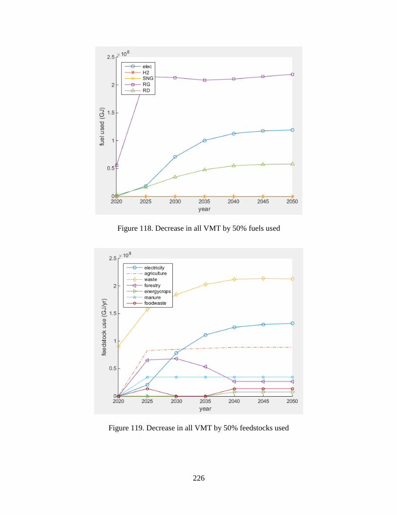
226

Figure 118. Decrease in all VMT by 50% fuels used

Figure 119. Decrease in all VMT by 50% feedstocks used

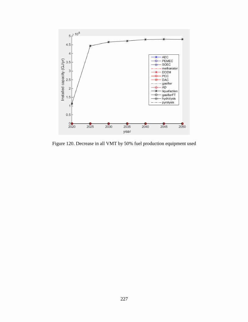
227

Figure 120. Decrease in all VMT by 50% fuel production equipment used

228

Figure 121. Decrease in all VMT by 50% fuel production equipment used

Increasing VMT also has the potential to drastically change adopted technologies,

depending on the magnitude of increase in VMT. Increasing VMT 10% for all years does not

affect technology adoption, but cumulative cost is increased by 10%. Increasing VMT 50% for

all years has a number of changes in technology adoptions as an increase in VMT makes meeting

emissions goals more stringent. For LDVs, ICVs are reduced while PHEVs and PFCEVs are

increased in later years. For linehaul HDVs, there is a majority of diesel-fueled HEVs for all

years with some diesel-fueled ICVs in 2035 and some BEVs in 2050. For drayage HDVs,

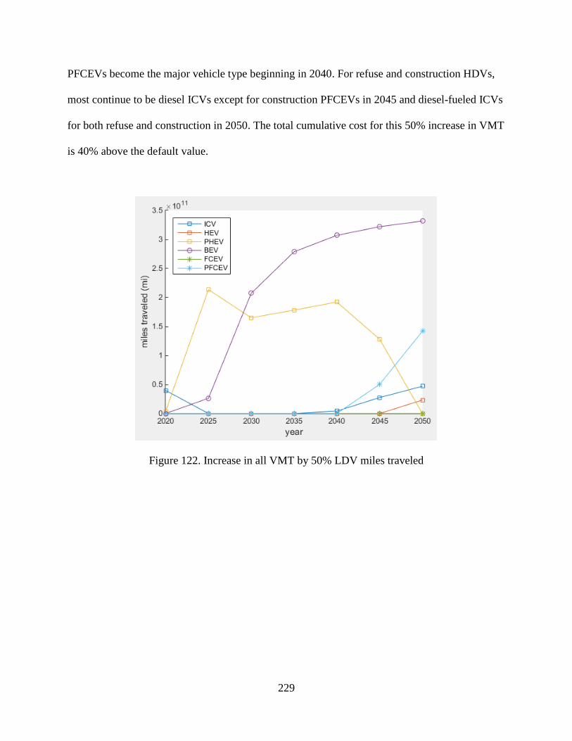
229

PFCEVs become the major vehicle type beginning in 2040. For refuse and construction HDVs,

most continue to be diesel ICVs except for construction PFCEVs in 2045 and diesel-fueled ICVs

for both refuse and construction in 2050. The total cumulative cost for this 50% increase in VMT

is 40% above the default value.

Figure 122. Increase in all VMT by 50% LDV miles traveled

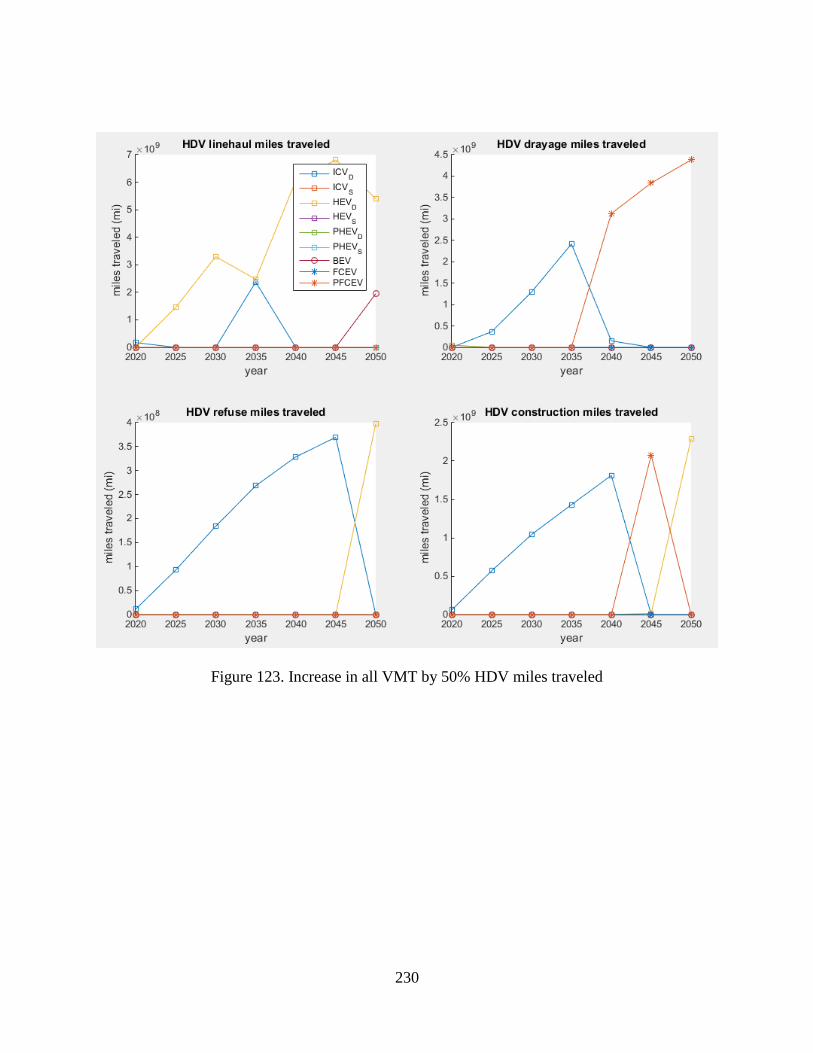
230

Figure 123. Increase in all VMT by 50% HDV miles traveled

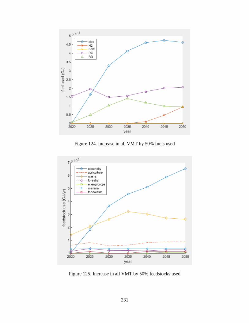
231

Figure 124. Increase in all VMT by 50% fuels used

Figure 125. Increase in all VMT by 50% feedstocks used

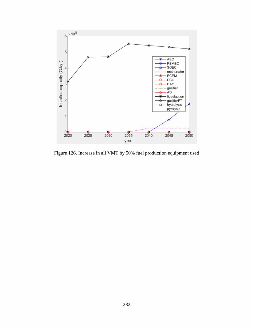
232

Figure 126. Increase in all VMT by 50% fuel production equipment used

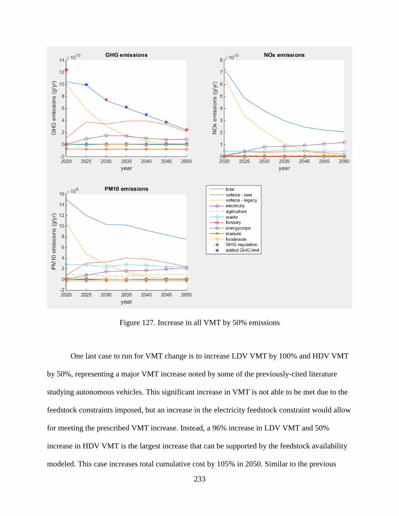
233

Figure 127. Increase in all VMT by 50% emissions

One last case to run for VMT change is to increase LDV VMT by 100% and HDV VMT

by 50%, representing a major VMT increase noted by some of the previously-cited literature

studying autonomous vehicles. This significant increase in VMT is not able to be met due to the

feedstock constraints imposed, but an increase in the electricity feedstock constraint would allow

for meeting the prescribed VMT increase. Instead, a 96% increase in LDV VMT and 50%

increase in HDV VMT is the largest increase that can be supported by the feedstock availability

modeled. This case increases total cumulative cost by 105% in 2050. Similar to the previous

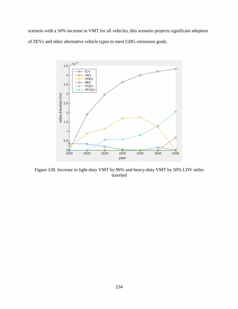
234

scenario with a 50% increase in VMT for all vehicles, this scenario projects significant adoption

of ZEVs and other alternative vehicle types to meet GHG emissions goals.

Figure 128. Increase in light-duty VMT by 96% and heavy-duty VMT by 50% LDV miles

traveled

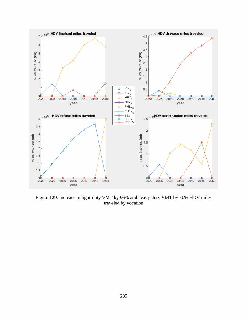
235

Figure 129. Increase in light-duty VMT by 96% and heavy-duty VMT by 50% HDV miles

traveled by vocation

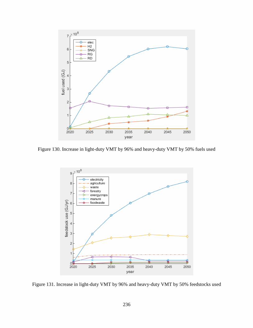
236

Figure 130. Increase in light-duty VMT by 96% and heavy-duty VMT by 50% fuels used

Figure 131. Increase in light-duty VMT by 96% and heavy-duty VMT by 50% feedstocks used

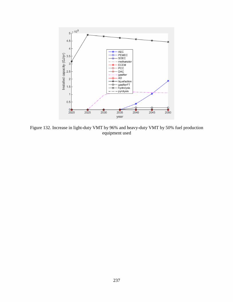
237

Figure 132. Increase in light-duty VMT by 96% and heavy-duty VMT by 50% fuel production

equipment used

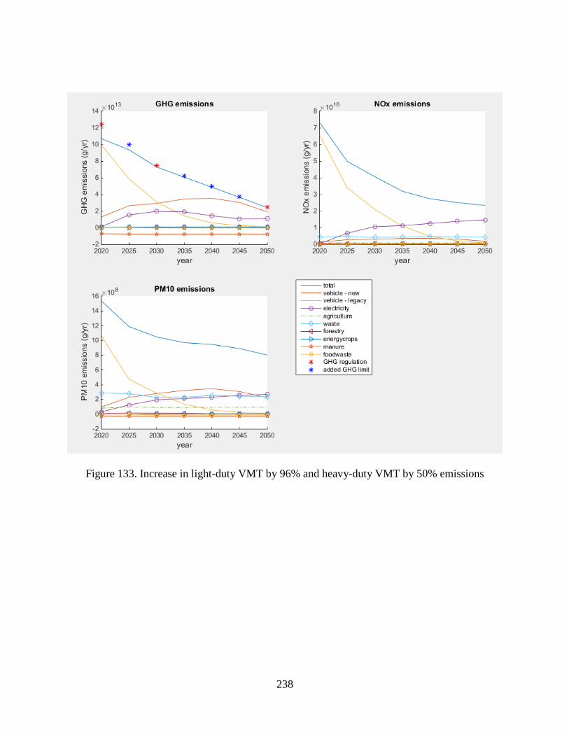
238

Figure 133. Increase in light-duty VMT by 96% and heavy-duty VMT by 50% emissions

239

9. SUMMARY AND CONCLUSIONS

9.1 Summary


configurations for LDVs and HDVs that meet environmental constraints at the lowest cost.

Achieving this goal was accomplished through reviewing related literature, finding major

research gaps, and formulating a methodology to fill those gaps. The literature review uncovered

two gaps relevant to the goal of this dissertation: 1) techno-economic study of alternative fuel

pathways and alternative vehicles is extensive, but studies that consider the combined fuel and

vehicle pathways with the various electricity and biomass feedstocks are absent; and 2) no work

has been conducted an optimization analysis of the various alternative fuel and vehicle

powertrain options that can be used to meet emissions goals. Addressing these two research gaps

formed the goal of this dissertation in order to project the optimal evolution of the transportation

sector to meet environmental and technical constraints.

Techno-economic analysis for the fuel pathways and powertrain configurations started

with data from the literature. Fuel production efficiencies and vehicle efficiencies obtained from

the literature were extrapolated when needed for advanced alternatives not yet on the market.

Technology costs from the literature were used with Wright’s Law and learning rates to project

future costs based on cumulative installed capacity. Fuel feedstock emission factor data from the

literature and emissions inventories combined with fuel pathway efficiency were used to

determine total fuel emissions. Vehicle emissions factors were sourced from emissions

inventories and vehicle testing certification.

Model constraints are GHG emissions, VMT, technology deployment rates, and fuel

feedstock availability. GHG emissions constraints come from California legislation and an

240

Executive Order, and CAP constraints from California Air Resources Board’s Mobile Source

Strategy. VMT projections, as well as the amount of VMT met by new vehicles included in the

present modeling, are from emissions inventories. Technology deployment constraints come

from various literature sources and U.S. Department of Energy future energy scenarios. Fuel

feedstock availability is from modeling in the literature and extensive U.S. Department of

Energy biomass characterization.

With the intention of using the preceding techno-economic data and constraints

described, an optimization problem was formulated using linear programming. This model,

named Transportation Rollout Affecting Cost and Emissions (TRACE), selects from available

fuel feedstocks, fuel production equipment technologies, fuel distribution methods, fuel

dispensing methods, and vehicle powertrain configurations that can use those fuels. TRACE has

the objective of selecting the lowest cost option of meeting transportation needs, both LDVs and

four major HDV vocations (linehaul, drayage, refuse, and construction), while meeting the

environmental and technical constraints previously detailed. The technology adoption choices

reduce future costs of those technologies based on Wright’s Law, affecting the results of the

proceeding optimization steps.

With the vast number of inputs to TRACE, including numerous efficiencies, costs,

learning rates, and emissions factors, sensitivity analyses provide insight into the major

components that have the largest impact on results. Some of these components include fuel

production technology costs, fuel distribution costs, vehicle costs, P2G plant capacity factors,

fuel feedstock costs, technology learning rates, and VMT projections. Note that all of the

previous factors are supply-side factors except for VMT projections which are demand-side

241

factors. Additionally, further constraints such as drayage CAP emissions and ZEV requirements

provide insight into the effect of these key scenarios that may face California in the near future.

9.2 Conclusions

9.2.1 LDV Conclusions

For the TRACE Non-ZEV Constrained Case, BEVs are a preferred LDV type in

2030 and beyond due to high fuel and vehicle pathway efficiency and moderate fuel

distribution and dispensing costs, while PFCEVs begin significant adoption in 2050.

While relatively high GHG emission factors generally discourage BEV use in early years

of modeling, SB 100 forces electric grid GHG emissions reductions in later years. These

emissions reductions, combined with very high fuel and vehicle pathway efficiency,

make light-duty BEVs a common choice in many of the cases run without a ZEV

constraint. PFCEVs have similar characteristics with higher overall costs, but can use

carbon-negative biomass while also providing driver conveniences such as long driving

range and short fueling time.

With constraints requiring ZEVs, PFCEVs as well as BEVs emerge as the preferred

options for LDVs.

A ZEV requirement that precludes the sale of any vehicle with an internal combustion

engine results in PFCEVs as well as BEVs being preferred for LDVs. PFCEVs achieve

the range and fueling times typical of today’s ICVs, and, along with BEVs, reduce GHGs

an additional 18% and CAPs up to an additional 40%.

242

9.2.2 HDV Conclusions

In the absence of ZEV constraints, ICVs, using renewable diesel produced by

liquefaction of biomass, are the preferred HDV until 2045 due to low vehicle cost,

low fuel feedstock cost, low fuel distribution and dispensing costs, and lower

efficiency benefit of alternative powertrains compared with LDVs. By 2050, HEVs

and PFCEVs are adopted for all modeled HDV vocations except refuse due to

tightening GHG emissions constraints.

HDVs travel significantly fewer miles than LDVs and therefore have less impact on

GHG emission reduction. Furthermore, efficiency benefits of alternative powertrains are

less significant for HDVs than LDVs, so the cost per mile is lower with the less

expensive conventional HDV powertrains than for much more expensive alternative

powertrains. In addition, the use of low cost distribution and existing dispensing

infrastructure for diesel fuel make renewable diesel-fueled ICVs a common choice for

HDVs in most of the cases run. By 2050, due to significantly tightened GHG emissions

constraints, all modeled HDV vocations except refuse begin adopting alternative

powertrains including HEVs and PFCEVs.

With additional constraints requiring ZEV options, PFCEVs are preferred for

HDVs due to efficiency and cost.

Imposing a ZEV requirement on HDVs leads to an HDV fleet of only PFCEVs. PFCEVs

offer high vehicle efficiency and are also modeled to have the lowest cost of heavy-duty

ZEVs. This is due to the powertrain specifications of a moderately sized battery and a

fuel cell that can be sized smaller than that for a FCEV due to the sizing of the battery.

243

While additional constraints on drayage NOx and PM10 tailpipe emissions do not

have a significant effect on the level of CAP emissions, the health impact of such

constraints may be significant.

Due to the relatively small number of miles traveled by drayage HDVs compared to

LDVs and other HDV vocations, the NOx and PM10 tailpipe emissions constraints from

California Air Resources Board’s Mobile Source Strategy for drayage trucks do not have

a significant impact on the total CAP emissions. NOx emissions reductions are 1.81% and

PM10 emissions reductions are 4.51% by 2050. However, CAPs are a local issue.

Therefore, the importance of utilizing PFCEVs for drayage should not be determined by

the percentage reduction of statewide CAPs they enable, but instead by the local CAP

reduction they enable at the ports, along freight corridors, and in nearby communities.

These local reductions lead to health improvements by those living in affected areas.

9.2.3 General Conclusions

Spending more money on alternative transportation technologies in early years can

lower total cumulative cost by 2050.

TRACE shows that spending more in the early years on alternative transportation

technologies can reduce the total amount of money spent in the future. It should be noted

that TRACE optimizes on each time step and not for total cost spent in the time horizon

of interest and, as a result, it is conceivable that even more money could be saved

compared to the Reference Case.

The TRACE Non-ZEV Constrained Case that meets environmental goals is 10%

less expensive than the Reference Case (i.e., business-as-usual fossil gasoline-fueled

244

light-duty ICVs in combination with a majority of fossil diesel-fueled heavy-duty

ICVs augmented with some fossil natural gas-fueled heavy-duty ICVs) by 2050.

Adoption of alternative fuels and alternative vehicle types can lead to lower cumulative

costs by 2050. The TRACE Non-ZEV Constrained Case LDV and HDV rollout case is

projected to cost $1.28 trillion by 2050, 10% less than the Reference Case. This would

require additional spending in early years, up to the year 2035, after which the alternative

choices using cleaner and significantly renewable fuels as well as alternative vehicles

reduces the cost of the transportation sector. While policy makers do not have to choose

between saving money and reducing emissions, they have to agree to spend more money

upfront.

Liquefaction is the preferred fuel production process due to a relatively high

efficiency, low VOM cost, and a low cost of accompanying fuel distribution and

dispensing as well as vehicle types.

Most TRACE cases select liquefaction as either the sole or major fuel production process

technology. As a method of producing liquid fuels from biomass, liquefaction takes

advantage of low-cost fuel distribution, existing fuel dispensing infrastructure, and low-

cost conventional ICVs. Compared with the other liquid fuel production technologies,

liquefaction has moderate capital cost but low VOM cost and high efficiency.

Battery cost has a significant impact on total cumulative cost of the transportation

sector.

Assuming no reduction in battery cost with increased production (a pessimistic but

realistic assumption if the same battery technologies are used in the next 30 years), total

245

cumulative cost of the modeled transportation sector increases by 22%. Therefore, if

projections for future battery costs do not predict much decline, this would mean

significantly higher cost for the transportation sector to meet emissions goals.

Both decreasing and increasing VMT have the potential to substantially change

adopted technologies depending on the amount of change in VMT.

If the future bodes a reduction in VMT for any number of reasons, the result is more

reliance on ICVs for LDVs and only ICVs for HDVs due to. An increase in VMT, which

could be spurred by the projected lower cost of transportation projected by TRACE

among other reasons, pushes the system to react to more VMT that must be met while

also complying with emissions constraints. This causes a shift in technology adoption

toward more expensive but also cleaner options such as electrolyzers, gasifiers, PFCEVs,

and BEVs.

The implementation of ZEV requirements results in adoption of light-duty PHEVs

as well as BEVs, and adoption of heavy-duty PFCEVs for all vocations with a net

result of 18% in additional GHG reductions, 6.6% reduction in NOx reductions, and

40% in PM10 reductions.

When imposing additional constraints to require only ZEV adoption, it is assumed that

heavy-duty ZEV options are available in 2020, which is optimistic for some powertrain

configurations and vocations. With such an imposition of constraints, LDVs are projected

to be BEVs and PFCEVs, and all HDVs of all vocations are projected to be PFCEVs. The

result is an overall increase in cost of 59% compared to without the ZEV requirement by

2050. This strategic adoption of ZEVs leads to 18% lower GHG emissions, 6.6% lower

246

NOx emissions, and 40% lower PM10 emissions compared to the absence of a ZEV

requirement. The resulting scenario yields GHG emissions levels 72.4% lower than

Executive Order S-3-05 requires in 2050.

TRACE determines the viability of alternative vehicle technologies and identifies the

contribution of each technology to meet environmental goals based on a set of

constraints. While the constraints analyzed in this dissertation are examples of

viable scenarios selected to demonstrate the utility and applicability of TRACE, the

results may vary for other scenarios selected for examination. TRACE is thereby a

tool for planning by identifying the portfolio of LDV and HDV vehicle technologies

and associated fuel supply streams required to meet, on an economic and emissions

basis, specific greenhouse gas and criteria air pollutant targets.

TRACE is a methodology that provides the means for identifying the portfolio of vehicle

technologies and fuel supply streams required to meet environmental goals, as well as

analyzing the cost and emissions impacts of any pre-determined scenario. The results of

this dissertation are based on the constraints that have been introduced to demonstrate

TRACE. Other sets of constraints may result in different fuel production and vehicle

technology rollouts. Furthermore, due to the nature of optimization, the results shown are

not necessarily the only viable options for meeting a given set of environmental targets.

9.3 Future Work

In general, future work should continue to update cost and efficiency projections as more

accurate and up-to-date data are determined. As more accurate data are made available,

projections into the future can also be made more accurate.

Further work on CAP emissions would benefit the results as well. More detailed emission

factors for the various biomass feedstocks, in particular those that are categorized as straws and

247

residues in this work that would ideally be individually specified, would allow for more accurate

CAP emissions calculations. Deeper investigation on the CAP emissions from the various fuel

production processes, fuel distribution, and fuel dispensing, instead of relying on feedstock

CAPs, would add greater detail and accuracy to CAP accounting. Lastly regarding CAPs, a

spatial accounting and air quality analysis would better capture the impact of resulting CAP

emissions changes compared to the CAP accounting of the present work.

The current talk of forestry biomass projections should be further investigated. The

Billion Ton Report projects a decline of forestry biomass in 2040 [31], while some forecast an

increase in dead and dying trees due to a number of issues such as wildfires and problematic

beetle infestations [313].

Similar to the technology rollout constraints for fuel production, there should be

analogous vehicle powertrain rollout constraints to ensure there is no unreasonable or impractical

increase of any vehicle technology. Some of the TRACE results recommend rapid switching of

vehicle technologies. While it may be true that vehicles generally have a shorter lifetime than

some fuel production plants, there should not be too drastic of changes in a five-year period of

time.

Additionally, material availability, particularly for batteries, fuel cells, and electrolyzers,

should be further studied and implemented as additional constraints. These would nicely

complement the technology deployment rate constraints and ensure that technologies

recommended are feasible to adopt.

The option to optimize with foresight (i.e. optimize the entire window of analysis at once

instead of optimizing each individual timestep) would change results and give the pathway with

the lowest total cumulative cost. This would also remove the need to apply artificial GHG

248

emissions constraints for the years that are not legislation or Executive Order. Additionally, this

foresight would better take advantage of Wright’s Law as currently, the cheapest option that

meets constraints is chosen even if choosing another may lead to lower cumulative cost in the

future. Both methods of optimization (that of the work of this dissertation as well as the proposed

method) have value, and adding the capability to do both would allow for other desired options

and further insight into the impact of these adoption choices.

249

10. REFERENCES

[1] C. C. D. US EPA, “Greenhouse Gas Emissions: Transportation Sector Emissions.” .

[2] US EPA, “Global Greenhouse Gas Emissions Data.” [Online]. Available:

https://www.epa.gov/ghgemissions/global-greenhouse-gas-emissions-data. [Accessed: 15-

Nov-2018].

[3] Oak Ridge National Laboratory, “Criteria Air Pollutants,” in Transportation Energy Data

Book: Edition 33, 2014, pp. 1–40.

[4] M. A. B. A. Tajudin et al., “Risk of concentrations of major air pollutants on the

prevalence of cardiovascular and respiratory diseases in urbanized area of Kuala Lumpur,

Malaysia,” Ecotoxicol. Environ. Saf., vol. 171, no. January 2019, pp. 290–300, 2019.

[5] S. O. Giwa, C. N. Nwaokocha, S. I. Kuye, and K. O. Adama, “Gas flaring attendant

impacts of criteria and particulate pollutants: A case of Niger Delta region of Nigeria,” J.

King Saud Univ. - Eng. Sci., vol. 31, no. 3, pp. 209–217, 2018.

[6] I. Seeni, S. Ha, C. Nobles, D. Liu, S. Sherman, and P. Mendola, “Air pollution exposure

during pregnancy: maternal asthma and neonatal respiratory outcomes,” Ann. Epidemiol.,

vol. 28, no. 9, pp. 612-618.e4, 2018.

[7] California Air Resources Board, “California Greenhouse Gas Emissions for 2000 to 2016:

Trends of Emissions and Other Indicators.” 2018.

[8] F. Pavley, “Assembly Bill 32.” [Online]. Available:

http://www.arb.ca.gov/cc/ab32/ab32.htm. [Accessed: 19-Jul-2016].

[9] F. Pavley, California Global Warming Solutions Act of 2006 (SB32), no. 32. 2006.

[10] A. Schwarzenegger, “Executive Order S-3-05.” 2005.

[11] Simitian, “Senate Bill 2.” 2011.

[12] K. De León, “Senate Bill No. 350: Clean Energy and Pollution Reduction Act of 2015.”

2015.

[13] K. De León, “Senate Bill No. 100 California Renewables Portfolio Standard Program:

emissions of greenhouse gases,” no. 100, 2018.

[14] D. Sherman, “2016 Toyota Mirai Fuel-Cell Sedan,” Car and Driver, 2015. [Online].

Available: http://www.caranddriver.com/toyota/mirai.

[15] California Air Resources Board, “Low Carbon Fuel Standard.” 2009.

[16] California Energy Commission; California Air Resrouces Board, “AB 1007.” 2007.

250

[17] Nunez, “Assembly Bill 118,” 2007. [Online]. Available:

http://www.arb.ca.gov/msprog/aqip/bkgrnd.htm.

[18] Office of Governor Edmund G. Brown Jr., “ZEV Action Plan,” 2013.

[19] Perea, Assembly Bill No. 8, no. 8. 2013, pp. 1–46.

[20] Lowenthal, “Senate Bill No. 1505,” no. 1505, 2006.

[21] E. Chau, “Assembly Bill No. 739.” 2017.

[22] E. Garcia, “Assembly Bill No. 1073.” 2017.

[23] California Air Resources Board, “Goods Movement Emission Reduction Plan,” 2015.

[Online]. Available: https://www.arb.ca.gov/bonds/gmbond/gmbond.htm. [Accessed: 22-

Feb-2018].

[24] “California Sustainable Freight Action Plan.” 2016.

[25] Clean Air Action Plan, “San Pedro Bay Ports Ready Cleaner Truck Rules for Oct. 1,”

2018. [Online]. Available: http://www.cleanairactionplan.org/2018/09/18/san-pedro-bay-

ports-ready-cleaner-truck-rules-for-oct-1/. [Accessed: 24-Jun-2019].

[26] B. Lane, B. Shaffer, and S. Samuelsen, “Plug-in fuel cell electric vehicles: A California

case study,” Int. J. Hydrogen Energy, vol. 42, no. 20, pp. 14294--14300, 2017.

[27] M. D. Fox, B. M. Geller, T. H. Bradley, F. R. Kalhammer, M. Bruce, and F. Panik, “Plug-

in Fuel Cell Vehicle Technology and Value Analysis,” World Electr. Veh. J., vol. 5, pp.

217–226, 2012.

[28] B. Tarroja, B. Shaffer, and S. Samuelsen, “The Importance of Grid Integration for

Achievable GHG Emissions Reductions from Alternative Vehicle Technologies,” 2014.

[29] EPRI, “Plug-in Fuel Cell Vehicle Technology and Value Analysis Phase 1: Preliminary

Findings and Plan for Detailed Study.” 2010.

[30] A. Pawlowski and D. Splitter, “SI Engine Trends : A Historical Analysis with Future

Projections,” SAE Tech. Pap., 2015.

[31] B. M. H. J. Langholtz, L. M. Stokes, and Eaton, “2016 BILLION-TON REPORT

Advancing Domestic Resources for a Thriving Bioeconomy,” Oak Ridge Natl. Lab., vol.

1160, no. July, pp. 448–2172, 2016.

[32] Energy and Environmental Economics, “Summary of the California State Agencies’

PATHWAYS Project: Long-Term GHG Reduction Scenarios,” 2016. [Online]. Available:

https://www.ethree.com/public_proceedings/summary-california-state-agencies-pathways-

project-long-term-greenhouse-gas-reduction-scenarios/. [Accessed: 07-Aug-2017].

[33] Argonne National Laboratory, “GREET Model.” [Online]. Available:

251

https://greet.es.anl.gov/. [Accessed: 11-Aug-2017].

[34] US Energy Information Administration, “Electric Power Monthly,” 2019. [Online].

Available: https://www.eia.gov/state/?sid=CA#tabs-4. [Accessed: 31-May-2019].

[35] R. Nikolewski, “Regulators vote to shut down Diablo Canyon, California’s last nuclear

power plant,” Los Angeles Times, 2018. [Online]. Available:

https://www.latimes.com/business/la-fi-diablo-canyon-nuclear-20180111-story.html.

[36] U.S. Energy Information Administration, “Electricity data browser - Argus Cogen Plant.”

[Online]. Available: https://www.eia.gov/electricity/data/browser/#/plant/10684.

[Accessed: 25-Jun-2019].

[37] L. Bertuccioli, A. Chan, D. Hart, F. Lehner, B. Madden, and E. Standen, “Development of

Water Electrolysis in the European Union Final Report Fuel cells and hydrogen,” 2014.

[38] Advanced Power and Energy Program, “The National Fuel Cell Research Center’s

Research and Development on ‘Power-to-Gas,’” 2015. [Online]. Available:

http://www.apep.uci.edu/NewsAndEvents/newsarchives/08272015-p2g.aspx. [Accessed:

25-Jun-2019].

[39] S. Wang, B. Tarroja, L. S. Schell, B. Shaffer, and S. Samuelsen, “Prioritizing among the

end uses of excess renewable energy for cost-effective greenhouse gas emission

reductions,” Appl. Energy, vol. 235, no. June 2018, pp. 284–298, 2019.

[40] US Environmental Protection Agency, “Biomass Combined Heat and Power Catalog of

Technologies,” no. September. 2007.

[41] L. Sentis et al., “Techno-economic analysis of UNIFHY hydrogem production system,”

2016.

[42] P. Spath, a Aden, T. Eggeman, M. Ringer, B. Wallace, and J. Jechura, “Biomass to

hydrogen production detailed design and economics utilizing the Battelle Columbus

laboratory indirectly heated gasifier,” no. NREL/TP-510-37408, 2005.

[43] F. S. Lau et al., “Techno-Economic Analysis of Hydrogen Production by Gasification of

Biomass,” 2002.

[44] E. D. Larson, H. Jin, and F. E. Celik, “Gasification-Based Fuels and Electricity Production

from Biomass, without and with Carbon Capture and Storage,” 2005.

[45] P. L. Spath, M. K. Mann, and W. A. Amos, “Update of Hydrogen from Biomass —

Determination of the Delivered Cost of Hydrogen,” 2003.

[46] M. Laser, E. Larson, B. Dale, M. Wang, N. Greene, and L. R. Lynd, “Comparative

analysis of efficiency, environmental impact, and process economics for mature biomass

refining scenarios,” Biofuels, Bioprod. Biorefining, no. 3, pp. 247–270, 2009.

252

[47] S. Sarkar and A. Kumar, “Biohydrogen production from forest and agricultural residues

for upgrading of bitumen from oil sands,” Energy, vol. 35, no. 2, pp. 582–591, 2010.

[48] C. N. Hamelinck and A. P. C. Faaij, “Future prospects for production of methanol and

hydrogen from biomass,” J. Power Sources, vol. 111, no. 1, pp. 1–22, 2002.

[49] N. Parker, Y. Fan, and J. Ogden, “From waste to hydrogen: An optimal design of energy

production and distribution network,” Transp. Res. Part E Logist. Transp. Rev., vol. 46,

no. 4, pp. 534–545, Jul. 2010.

[50] R. E. Katofsky, “The Production of Fluid Fuels From Biomass,” Princeton University,

Princeton, 1993.

[51] A. Corradetti and U. Desideri, “Should Biomass be Used for Power Generation or

Hydrogen Production?,” J. Eng. Gas Turbines Power, vol. 129, no. 3, p. 629, 2007.

[52] L. Tock and F. Maréchal, “Co-production of hydrogen and electricity from lignocellulosic

biomass: Process design and thermo-economic optimization,” Energy, vol. 45, no. 1, pp.

339–349, 2012.

[53] Department of Energy, “Hydrogen Production: Natural Gas Reforming.” [Online].

Available: http://energy.gov/eere/fuelcells/hydrogen-production-natural-gas-reforming.

[Accessed: 06-May-2016].

[54] H. Abdi, B. Mohammadi-ivatloo, S. Javadi, R. Khodaei, and E. Dehnavi, “Energy Storage

Systems,” in Distributed Generation Systems, 2017, pp. 333–368.

[55] K. Stangeland, D. Kalai, H. Li, and Z. Yu, “CO 2 Methanation: The Effect of Catalysts

and Reaction Conditions,” Energy Procedia, vol. 105, no. 1876, pp. 2022–2027, 2017.

[56] J. Ralston, “The Sabatier Reaction, Possible Solution to CO2 Emissions - PennEnergy,”

PennEnergy, 2010. [Online]. Available:

http://www.pennenergy.com/articles/pennenergy/2010/03/the-sabatier-reaction.html.

[Accessed: 10-Oct-2017].

[57] A. Maroufmashat and M. Fowler, “Transition of future energy system infrastructure;

through power-to-gas pathways,” Energies, vol. 10, no. 8, 2017.

[58] T. Schaaf, J. Grünig, M. R. Schuster, T. Rothenfluh, and A. Orth, “Methanation of CO2 -

storage of renewable energy in a gas distribution system,” Energy. Sustain. Soc., vol. 4,

no. 1, p. 2, 2014.

[59] NASA, “Chemical Equilibrium with Applications (CEA).” [Online]. Available:

https://www.grc.nasa.gov/www/CEAWeb/. [Accessed: 31-Jan-2018].

[60] M. Götz et al., “Renewable Power-to-Gas: A technological and economic review,” Renew.

Energy, vol. 85, pp. 1371–1390, 2016.

253

[61] M. De Saint Jean, P. Baurens, C. Bouallou, and K. Couturier, “Economic assessment of a

power-to-substitute-natural-gas process including high-temperature steam electrolysis,”

Int. J. Hydrogen Energy, vol. 40, no. 20, pp. 6487–6500, 2015.

[62] A. El Sibai, L. K. Rihko Struckmann, and K. Sundmacher, “Model-based Optimal

Sabatier Reactor Design for Power-to-Gas Applications,” Energy Technol., vol. 5, no. 6,

pp. 911–921, 2017.

[63] P. Collet et al., “Techno-economic and Life Cycle Assessment of methane production via

biogas upgrading and power to gas technology,” Appl. Energy, vol. 192, pp. 282–295,

2017.

[64] Z. Pan, Q. Liu, L. Zhang, J. Zhou, C. Zhang, and S. H. Chan, “Experimental and

thermodynamic study on the performance of water electrolysis by solid oxide electrolyzer

cells with Nb-doped Co-based perovskite anode,” Appl. Energy, vol. 191, pp. 559–567,

2017.

[65] M. Bailera, P. Lisbona, L. M. Romeo, and S. Espatolero, “Power to Gas projects review:

Lab, pilot and demo plants for storing renewable energy and CO2,” Renew. Sustain.

Energy Rev., vol. 69, no. January 2016, pp. 292–312, 2017.

[66] A. Pääkkönen, H. Tolvanen, and J. Rintala, “Techno-economic analysis of a power to

biogas system operated based on fluctuating electricity price,” Renew. Energy, vol. 117,

pp. 166–174, 2017.

[67] L. Wang, M. Pérez-Fortes, H. Madi, S. Diethelm, J. Van herle, and F. Maréchal, “Optimal

design of solid-oxide electrolyzer based power-to-methane systems: A comprehensive

comparison between steam electrolysis and co-electrolysis,” Appl. Energy, vol. 211, no.

December 2017, pp. 1060–1079, 2018.

[68] U.S. Department of Energy, “Post-Combustion Carbon Capture Research.” [Online].

Available: https://energy.gov/fe/science-innovation/carbon-capture-and-storage-

research/carbon-capture-rd/post-combustion-carbon. [Accessed: 10-Oct-2017].

[69] National Energy Technology Laboratory, “Post-Combustion CO2 Capture.” [Online].

Available: https://www.netl.doe.gov/research/coal/carbon-capture/post-combustion.

[Accessed: 28-Jan-2018].

[70] R. Socolow et al., “Direct Air Capture of CO 2 with Chemicals: A Technology

Assessment for the APS Panel on Public Affairs,” American Physical Society. p. 100,

2011.

[71] D. Parry, “NRL Seawater Carbon Capture Process Receives U.S. Patent,” US Naval

Research Laboratory, 2016.

[72] H. D. Willauer, D. R. Hardy, and F. W. Williams, “The Feasibility and Current Estimated

Capital Costs of Producing Jet Fuel at Sea Using Carbon Dioxide and Hydrogen.” US

Naval Research Laboratory, 2010.

254

[73] Y. Zhang and M. Goldberg, “Jobs and Economic Development Impact ( JEDI ) User

Reference Guide : Fast Pyrolysis Biorefinery Model,” no. March. NREL, 2015.

[74] US EPA, “Frequent Questions about Anaerobic Digestion.” [Online]. Available:

https://www.epa.gov/anaerobic-digestion/frequent-questions-about-anaerobic-digestion.

[Accessed: 30-May-2019].

[75] S. Jones et al., “Process design and economics for the conversion of lignocellulosic

biomass to hydrocarbon fuels: Fast pyrolysis and hydrotreating bio-oil pathway,” 2013.

[76] F. Kabir Kazi, J. Fortman, and R. Anex, “Techno-Economic Analysis of Biochemical

Scenarios for Production of Cellulosic Ethanol Techno-Economic Analysis of

Biochemical Scenarios for Production of Cellulosic Ethanol,” 2010.

[77] D. Humbird et al., “Process Design and Economics for Biochemical Conversion of

Lignocellulosic Biomass to Ethanol: Dilute-Acid Pretreatment and Enzymatic Hydrolysis

of Corn Stover,” 2011.

[78] R. Davis et al., “Process Design and Economics for the Conversion of Algal Biomass to

Biofuels: Algal Biomass Fractionation to Lipid- and Carbohydrate-Derived Fuel

Products,” no. September, 2014.

[79] N. C. Parker, J. M. Ogden, and Y. Fan, “The role of biomass in California’s hydrogen

economy,” Energy Policy, vol. 36, no. 10, pp. 3925–3939, 2008.

[80] Z. Liu, J. M. Norbeck, A. S. K. Raju, S. Kim, and C. S. Park, “Synthetic natural gas

production by sorption enhanced steam hydrogasification based processes for improving

CH 4 yield and mitigating CO 2 emissions,” Energy Convers. Manag., vol. 126, pp. 256–

265, 2016.

[81] T. Bridgwater, “Biomass for energy,” J. Sci. Food Agric., vol. 86, no. 12, pp. 1755–1768,

2006.

[82] CR&R, “CR&R Anaerobic Digestion Facility Renewable Fuel from Organic Waste

Recycling - Organics Infrastructure Development in California.” 2018.

[83] Z. Zahan and M. Z. Othman, “Effect of pre-treatment on sequential anaerobic co-digestion

of chicken litter with agricultural and food wastes under semi-solid conditions and

comparison with wet anaerobic digestion,” Bioresour. Technol., vol. 281, no. January, pp.

286–295, 2019.

[84] S. A. Gebrezgabher, M. P. M. Meuwissen, B. A. M. Prins, and A. G. J. M. Oude Lansink,

“Economic analysis of anaerobic digestion - A case of Green power biogas plant in The

Netherlands,” NJAS - Wageningen J. Life Sci., vol. 57, pp. 109–115, 2010.

[85] US Environmental Protection Agency, “Basic Information about Anaerobic Digestion

(AD).” [Online]. Available: https://www.epa.gov/anaerobic-digestion/basic-information-

about-anaerobic-digestion-ad. [Accessed: 25-Jun-2019].

255

[86] J. Herguido, J. Corella, and J. González-Saiz, “Steam Gasification of Lignocellulosic

Residues in a Fluidized Bed at a Small Pilot Scale. Effect of the Type of Feedstock,” Ind.

Eng. Chem. Res., vol. 31, no. 5, pp. 1274–1282, 1992.

[87] A. Molino and G. Braccio, “Synthetic natural gas SNG production from biomass

gasification - Thermodynamics and processing aspects,” Fuel, vol. 139, pp. 425–429,

2015.

[88] M. Gassner and F. Maréchal, “Thermo-economic optimisation of the polygeneration of

synthetic natural gas (SNG), power and heat from lignocellulosic biomass by gasification

and methanation,” Energy Environ. Sci., vol. 5, no. 2, pp. 5768–5789, 2012.

[89] A. Galvagno, M. Prestipino, V. Chiodo, S. Maisano, S. Brusca, and R. Lanzafame,

“Energy Performance of CHP System Integrated with Citrus Peel Air-Steam Gasification:

A Comparative Study,” Energy Procedia, vol. 126, pp. 485–492, 2017.

[90] F. Feng, G. H. Song, L. H. Shen, and J. Xiao, “Energy efficiency analysis of biomass-

based synthetic natural gas production process using interconnected fluidized beds and

fluidized bed methanation reactor,” Clean Technol. Environ. Policy, vol. 18, no. 3, pp.

965–971, 2016.

[91] G. Song, F. Feng, J. Xiao, and L. Shen, “Technical assessment of synthetic natural gas

(SNG) production from agriculture residuals,” J. Therm. Sci., vol. 22, no. 4, pp. 359–365,

2013.

[92] A. Alamia, I. Magnusson, F. Johnsson, and H. Thunman, “Well-to-wheel analysis of bio-

methane via gasification, in heavy duty engines within the transport sector of the

European Union,” Appl. Energy, vol. 170, no. 2016, pp. 445–454, 2016.

[93] E. Fahlén and E. O. Ahlgren, “Assessment of integration of different biomass gasification

alternatives in a district-heating system,” Energy, vol. 34, no. 12, pp. 2184–2195, 2009.

[94] G. Song, J. Xiao, Y. Yu, and L. Shen, “A techno-economic assessment of SNG production

from agriculture residuals in China,” Energy Sources, Part B Econ. Plan. Policy, vol. 11,

no. 5, pp. 465–471, 2016.

[95] M. Gassner and F. Maréchal, “Methodology for the optimal thermo-economic, multi-

objective design of thermochemical fuel production from biomass,” Comput. Chem. Eng.,

vol. 33, no. 3, pp. 769–781, 2009.

[96] A. Duret, C. Friedli, and M. Francois, “Prosess design of Synthetic Natural Gas (SNG)

production using gasification.” .

[97] M. T. Johansson, “Bio-synthetic natural gas as fuel in steel industry reheating furnaces - A

case study of economic performance and effects on global CO2emissions,” Energy, vol.

57, pp. 699–708, 2013.

[98] S. Wang, X. Bi, and S. Wang, “Thermodynamic analysis of biomass gasification for

256

biomethane production,” Energy, vol. 90, pp. 1207–1218, 2015.

[99] H. Gu, G. Song, J. Xiao, H. Zhao, and L. Shen, “Thermodynamic Analysis of the

Biomass-to-Synthetic Natural Gas Using Chemical Looping Technology with CaO

Sorbent,” Energy & Fuels, vol. 27, no. 8, pp. 4695–4704, 2013.

[100] M. Mozaffarian and Z. R.W.R., “Feasibility Of Biomass / Waste-Related SNG Production

Technologies Final report,” 2003.

[101] G. Haarlemmer, G. Boissonnet, E. Peduzzi, and P. A. Setier, “Investment and production

costs of synthetic fuels - A literature survey,” Energy, vol. 66, pp. 667–676, 2014.

[102] H. Li, E. Larsson, E. Thorin, E. Dahlquist, and X. Yu, “Feasibility study on combining

anaerobic digestion and biomass gasification to increase the production of biomethane,”

Energy Convers. Manag., vol. 100, pp. 212–219, 2015.

[103] B. M. Jenkins, J. F. Arthur, G. E. Miller, and P. S. Parsons, “Logistics and economics of

biomass utilization,” Trans. ASAE, vol. 27, no. 6, pp. 1898–1904, 1984.

[104] M. C. Seemann, T. J. Schildhauer, and S. M. A. Biollaz, “Erratum: Fluidized bed

methanation of wood-derived producer gas for the production of synthetic natural gas

(Industrial and Engineering Chemistry Research 49:21 (7034-7038)),” Ind. Eng. Chem.

Res., vol. 49, no. 21, p. 11119, 2010.

[105] S. Rönsch et al., “Review on methanation - From fundamentals to current projects,” Fuel,

vol. 166, pp. 276–296, 2016.

[106] K. Difs, E. Wetterlund, L. Trygg, and M. Söderström, “Biomass gasification opportunities

in a district heating system,” Biomass and Bioenergy, vol. 34, no. 5, pp. 637–651, 2010.

[107] S. Li, H. Jin, L. Gao, and X. Zhang, “Exergy analysis and the energy saving mechanism

for coal to synthetic/substitute natural gas and power cogeneration system without and

with CO2capture,” Appl. Energy, vol. 130, pp. 552–561, 2014.

[108] S. Heyne, H. Thunman, and S. Harvey, “Extending existing combined heat and power

plants for synthetic natural gas production,” Int. Agric. Eng. J., vol. 23, no. 2, pp. 70–79,

2012.

[109] C. R. Vitasari, M. Jurascik, and K. J. Ptasinski, “Exergy analysis of biomass-to-synthetic

natural gas (SNG) process via indirect gasification of various biomass feedstock,” Energy,

vol. 36, no. 6, pp. 3825–3837, 2011.

[110] L. Zhu, L. Zhang, J. Fan, P. Jiang, and L. Li, “MSW to synthetic natural gas: System

modeling and thermodynamics assessment,” Waste Manag., vol. 48, pp. 257–264, 2016.

[111] R. W. R. Zwart and H. Boerrigter, “High efficiency co-production of synthetic natural gas

(SNG) and Fischer-Tropsch (FT) transportation fuels from biomass,” Energy and Fuels,

vol. 19, no. 2, pp. 591–597, 2005.

257

[112] C. M. van der Meijden, H. J. Veringa, and L. P. L. M. Rabou, “The production of

synthetic natural gas (SNG): A comparison of three wood gasification systems for energy

balance and overall efficiency,” Biomass and Bioenergy, vol. 34, no. 3, pp. 302–311,

2010.

[113] J. Song, W. Yang, Y. Higano, and X. Wang, “Dynamic integrated assessment of

bioenergy technologies for energy production utilizing agricultural residues: An input-

output approach,” Appl. Energy, vol. 158, pp. 178–189, 2015.

[114] L. E. Arteaga-Pérez, O. Gómez-Cápiro, A. Karelovic, and R. Jiménez, “A modelling

approach to the techno-economics of Biomass-to-SNG/Methanol systems: Standalone vs

Integrated topologies,” Chem. Eng. J., vol. 286, pp. 663–678, 2016.

[115] J. Kopyscinski, T. J. Schildhauer, and S. M. A. Biollaz, “Production of synthetic natural

gas (SNG) from coal and dry biomass - A technology review from 1950 to 2009,” Fuel,

vol. 89, no. 8, pp. 1763–1783, 2010.

[116] L. Axelsson, M. Franzén, M. Ostwald, G. Berndes, G. Lakshmi, and N. H. Ravindranath,

“Perspective: Jatropha cultivation in southern India: Assessing farmers’ experiences,”

Biofuels, Bioprod. Biorefining, vol. 6, no. 3, pp. 246–256, 2012.

[117] G. W. Huber, S. Iborra, and A. Corma, “Synthesis of transportation fuels from biomass:

Chemistry, catalysts, and engineering,” Chem. Rev., vol. 106, no. 9, pp. 4044–4098, 2006.

[118] P. McKendry, “Energy production from biomass (part 1): Overview of biomass,”

Bioresour. Technol., vol. 83, no. 1, pp. 37–46, 2002.

[119] D. M. Alonso, J. Q. Bond, and J. A. Dumesic, “Catalytic conversion of biomass to bio-

syncrude oil,” Green Chem., no. 12, pp. 1493–1513, 2010.

[120] Y. Zhu, S. Tjokro Rahardjo, C. Valkenburg, L. Snowden-Swan, S. Jones, and M.

Machinal, “Techno-economic Analysis for the Thermochemical Conversion of Biomass to

Liquid Fuels (U.S. DOE),” Doe, no. June, p. 152, 2011.

[121] C. Yang, J. Wu, Z. Deng, B. Zhang, C. Cui, and Y. Ding, “A Comparison of Energy

Consumption in Hydrothermal Liquefaction and Pyrolysis of Microalgae,” Trends Renew.

Energy, vol. 3, no. 1, pp. 76–85, 2017.

[122] National Energy Technology Laboratory, “Fischer-Tropsch Synthesis.” [Online].

Available: https://www.netl.doe.gov/research/coal/energy-

systems/gasification/gasifipedia/ftsynthesis. [Accessed: 09-Jun-2019].

[123] US Energy Information Administration, “How Electricity Is Delivered To Consumers -

Energy Explained, Your Guide To Understanding Energy,” 2018. [Online]. Available:

https://www.eia.gov/energyexplained/index.php?page=electricity_delivery. [Accessed:

12-May-2019].

[124] C. Cao, L. Wang, and B. Chen, “Mitigation of the impact of high plug-in electric vehicle

258

penetration on residential distribution grid using smart charging strategies,” Energies, vol.

9, no. 12, 2016.

[125] Eric Wesoff, “How Big an Impact Will EVs Have on the Grid and Your Wallet?,”

Greentech Media, 2013. [Online]. Available:

https://www.greentechmedia.com/articles/read/how-big-an-impact-will-evs-have-on-the-

grid-and-your-wallet. [Accessed: 09-Aug-2017].

[126] M. W. Melaina, O. Antonia, and M. Penev, “Blending Hydrogen into Natural Gas Pipeline

Networks: A Review of Key Issues,” 2013.

[127] US DRIVE, “Hydrogen Delivery Technical Team Roadmap,” U.S. Drive, Driv. Res.

Innov. Veh. Effic. Energy Sustain., no. June, p. 30, 2013.

[128] CPUC, “Decision Regarding the Costs of Compliance with Decision 14-01-034 and

Adoption of Biomethane Promotion Policies and Program,” Public Utilities Commission

of the State of California. R.13-02-008. Available at:

http://docs.cpuc.ca.gov/PublishedDocs/Published/G000/M152/K572/152572023.PDF,

2015.

[129] US Department of Energy, “Vehicle Charging.” [Online]. Available:

https://www.energy.gov/eere/electricvehicles/vehicle-charging. [Accessed: 10-Jun-2019].

[130] Rob Stumpf, “Porsche Taycan Can Add 62 Miles of Driving Range in 4-Minute Charge,”

The Drive, 2018. [Online]. Available: https://www.thedrive.com/news/25136/porsche-

taycan-can-add-62-miles-of-driving-range-in-just-4-minutes. [Accessed: 26-Jun-2019].

[131] X. Lin, X. Hao, Z. Liu, and W. Jia, “Health conscious fast charging of Li-ion batteries via

a single particle model with aging mechanisms,” J. Power Sources, vol. 400, no. August,

pp. 305–316, 2018.

[132] J. Sieg et al., “Fast charging of an electric vehicle lithium-ion battery at the limit of the

lithium deposition process,” J. Power Sources, vol. 427, no. March, pp. 260–270, 2019.

[133] California Fuel Cell Partnership, “California Hydrogen Stations.” 2019.

[134] U.S. Department of Energy, “Fact of the Month #18-01, January 29: There Are 39

Publicly Available Hydrogen Fueling Stations in the United States.” [Online]. Available:

https://www.energy.gov/eere/fuelcells/fact-month-18-01-january-29-there-are-39-

publicly-available-hydrogen-fueling-stations. [Accessed: 26-Jun-2019].

[135] K. Reddi, M. Mintz, A. Elgowainy, and E. Sutherland, 13 - Building a hydrogen

infrastructure in the United States. Elsevier Ltd., 2016.

[136] US Department of Energy, “Natural Gas Fueling Station Locations.” [Online]. Available:

https://afdc.energy.gov/fuels/natural_gas_locations.html#/analyze?fuel=CNG&region=US

-CA&cng_vehicle_class=HD. [Accessed: 18-Jun-2019].

259

[137] P. Couch, “Personal Communication, Patrick Couch, Vice President of Technical

Services, June 19.” Gladstein Neandross & Associates, 2019.

[138] US Department of Energy, “Alternative Fuels Data Center: Compressed Natural Gas

Fueling Stations.” [Online]. Available:

https://afdc.energy.gov/fuels/natural_gas_cng_stations.html. [Accessed: 12-Jun-2019].

[139] M. R. Swain, J. Shriber, and M. N. Swain, “Comparison of hydrogen, natural gas,

liquified petroleum gas, and gasoline leakage in a residential garage,” Energy and Fuels,

vol. 12, no. 1, pp. 83–89, 1998.

[140] US Department of Energy, “Alternative Fuels Data Center: Maps and Data - Average

Annual Vehicle Miles Traveled of Major Vehicle Categories,” 2018. [Online]. Available:

https://afdc.energy.gov/data/10309. [Accessed: 19-Jun-2019].

[141] ARB, “EMFAC2017 Web Database,” 2019. [Online]. Available:

https://www.arb.ca.gov/emfac/2017/. [Accessed: 02-Jun-2019].

[142] California New Car Dealers Association, “California Green Vehicle Report,” no. August,

p. 3, 2018.

[143] P. Margalef, T. M. Brown, J. Brouwer, and S. Samuelsen, “Efficiency comparison of tri-

generating HTFC to conventional hydrogen production technologies,” Int. J. Hydrogen

Energy, vol. 37, no. 12, pp. 9853–9862, 2012.

[144] California Air Resources Board, “Vision Scenario Planning,” 2017. [Online]. Available:

https://www.arb.ca.gov/planning/vision/vision.htm. [Accessed: 07-Nov-2018].

[145] CA Air Resources Board, “Heavy-Duty Low NOx,” 2019. [Online]. Available:

https://www.arb.ca.gov/msprog/hdlownox/hdlownox.htm. [Accessed: 13-Jun-2019].

[146] California Natural Gas Vehicle Partnership, “Ultra-Low Emission Engines.” [Online].

Available: https://cngvp.org/why-natural-gas/ultra-low-nox-engines/. [Accessed: 13-Jun-

2019].

[147] US Department of Energy, “The History of the Electric Car,” 2014. [Online]. Available:

https://energy.gov/articles/history-electric-car. [Accessed: 08-Sep-2017].

[148] J. D. Power, “History of the Hybrid Car,” 2012. [Online]. Available:

http://www.jdpower.com/cars/articles/safety-and-mpg/history-hybrid-car. [Accessed: 08-

Sep-2015].

[149] CA EPA Air Resources Board, “Zero-Emission Vehicle Regulatory and Legal Activities,”

2011. [Online]. Available: http://www.arb.ca.gov/msprog/zevprog/background.htm.

[Accessed: 09-Sep-2015].

[150] C. H. Stephan, C. H. Stephan, J. Sullivan, and J. Sullivan, “Environmental and energy

implications of plug‐in hybrid‐ electric vehicles,” Environ. Sci. Technol., vol. 42, no. 4, p.

260

1185‐1190, 2008.

[151] Inside EVs, “Monthly Plug-In Sales Scorecard,” 2016. [Online]. Available:

http://insideevs.com/monthly-plug-in-sales-scorecard/. [Accessed: 21-Jun-2016].

[152] S. Manzetti and F. Mariasiu, “Electric vehicle battery technologies: From present state to

future systems,” Renew. Sustain. Energy Rev., vol. 51, pp. 1004–1012, 2015.

[153] Chevrolet, “2017 Bolt EV,” 2017. [Online]. Available: http://www.chevrolet.com/bolt-ev-

electric-vehicle. [Accessed: 05-Aug-2017].

[154] Tesla, “Model 3,” 2017. [Online]. Available: https://www.tesla.com/model3. [Accessed:

05-Aug-2017].

[155] Z. Zhang, H. Xu, L. Shi, D. Li, and Y. Han, “Application research of an electric vehicle

DC fast charger in smart grids,” ICIAFS 2012 - Proc. 2012 IEEE 6th Int. Conf. Inf. Autom.

Sustain., pp. 258–261, 2012.

[156] US Energy Information Administration, “Carbon intensity of energy use is lowest in U.S.

industrial and electric power sectors,” 2017. [Online]. Available:

https://www.eia.gov/todayinenergy/detail.php?id=31012. [Accessed: 10-Sep-2017].

[157] ARB, “Draft Technology Assessment: Medium- and Heavy-Duty Battery Electric Trucks

and Buses,” no. October. 2015.

[158] US Department of Energy, “Types of Fuel Cells.” [Online]. Available:

https://energy.gov/eere/fuelcells/types-fuel-cells. [Accessed: 08-Aug-2017].

[159] California Energy Commission, “Energy Commission Approves $8 Million Grant for

Hydrogen Fuel Cell Station at Port of Long Beach,” 2018. [Online]. Available:

https://www.energy.ca.gov/releases/2018_releases/2018-11-07_hydrogen_station_nr.html.

[Accessed: 08-Nov-2018].

[160] Mercedes-Benz, “The Mercedes-Benz GLC F-Cell.” [Online]. Available:

https://www.mbusa.com/mercedes/future/model/model-

Mercedes_Benz_GLC_F_Cell#module=future-gallery&submodule=future-gallery-

0&gallery=UNIQUE-GALLERY-ID%7C0%7C0. [Accessed: 07-Jun-2019].

[161] S. Salisbury, B. Geller, T. Bradley, and M. Fox, “Detailed Design of a Fuel Cell Plug-in

Hybrid Electric Vehicle,” SAE Int., 2013.

[162] J. P. Ribau, C. M. Silva, and J. M. C. Sousa, “Efficiency, cost and life cycle CO2

optimization of fuel cell hybrid and plug-in hybrid urban buses,” Appl. Energy, vol. 129,

pp. 320–335, 2014.

[163] G. J. Offer, D. Howey, M. Contestabile, R. Clague, and N. P. Brandon, “Comparative

analysis of battery electric, hydrogen fuel cell and hybrid vehicles in a future sustainable

road transport system,” Energy Policy, vol. 38, no. 1, pp. 24–29, 2010.

261

[164] S. Kelouwani, K. Agbossou, Y. Dubé, and L. Boulon, “Fuel cell plug-in hybrid electric

vehicle anticipatory and real-time blended-mode energy management for battery life

preservation,” J. Power Sources, vol. 221, pp. 406–418, 2013.

[165] J. D. Bucher and T. H. Bradley, “Modeling operating modes, energy consumptions, and

infrastructure requirements of fuel cell plug in hybrid electric vehicles using longitudinal

geographical transportation data,” Int. J. Hydrogen Energy, vol. 43, no. 27, pp. 12420–

12427, 2018.

[166] F. Syed, M. Fowler, D. Wan, and Y. Maniyali, “An energy demand model for a fleet of

plug-in fuel cell vehicles and commercial building interfaced with a clean energy hub,”


[167] US Department of Energy, “Alternative Fuels Data Center: Filling CNG Fuel Tanks.”

[Online]. Available: https://afdc.energy.gov/vehicles/natural_gas_filling_tanks.html.


[168] Lawrence Livermore National Laboratory, “Energy Flow Charts,” 2018. [Online].

Available: https://flowcharts.llnl.gov/. [Accessed: 08-Nov-2018].

[169] L. Bertuccioli, A. Chan, D. Hart, F. Lehner, B. Madden, and E. Standen, “Development of

water electrolysis in the EU,” Fuel Cells Hydrog. Jt. Undert., no. February, pp. 1–160,

2014.

[170] O. Schmidt, A. Gambhir, I. Staffell, A. Hawkes, J. Nelson, and S. Few, “Future cost and

performance of water electrolysis: An expert elicitation study,” Int. J. Hydrogen Energy,

vol. 42, no. 52, pp. 30470–30492, 2017.

[171] T. Ramsden, M. Ruth, V. Diakov, M. Laffen, and T. Timbario, “Hydrogen Pathways:

Updated Cost, Well-to-Wheels Energy Use, and Emissions for the Current Technology

Status of Ten Hydrogen Production, Delivery, and Distribution Scenarios,” DoE EERE,

no. September, 2013.

[172] J. Eichman, A. Townsend, and M. Melaine, “Economic Assessment of Hydrogen

Technologies Participating in California Electricity Markets,” Natl. Renew. Energy Lab.,

no. February, p. 31, 2016.

[173] M. Melaina and J. Eichman, “Hydrogen Energy Storage: Grid and Transportation Services

(Technical Report),” NREL (National Renew. Energy Lab., no. February, p. Medium: ED;

Size: 66 pp., 2015.

[174] S. Campanari, G. Manzolini, and F. Garcia de la Iglesia, “Energy analysis of electric

vehicles using batteries or fuel cells through well-to-wheel driving cycle simulations,” J.

Power Sources, vol. 186, no. 2, pp. 464–477, 2009.

[175] P. Bolat and C. Thiel, “Hydrogen supply chain architecture for bottom-up energy systems

models. Part 2: Techno-economic inputs for hydrogen production pathways,” Int. J.

Hydrogen Energy, vol. 39, no. 17, pp. 8898–8925, 2014.

262

[176] W. Krewitt and S. Schmid, “Fuel Cell Technologies and Hydrogen

Production/Distribution Options,” DLR, no. September, pp. 1–113, 2005.

[177] M. Robinius et al., “Power-to-Gas: Electrolyzers as an alternative to network expansion –

An example from a distribution system operator,” Appl. Energy, vol. 210, no. May 2017,

pp. 182–197, 2018.

[178] C. Wulf et al., “Life Cycle Assessment of hydrogen transport and distribution options,” J.

Clean. Prod., vol. 199, pp. 431–443, 2018.

[179] A. S. Snehesh, H. S. Mukunda, S. Mahapatra, and S. Dasappa, “Fischer-Tropsch route for

the conversion of biomass to liquid fuels - Technical and economic analysis,” Energy, vol.

130, pp. 182–191, 2017.

[180] S. Hänggi et al., “A review of synthetic fuels for passenger vehicles,” Energy Reports,

vol. 5, pp. 555–569, 2019.

[181] F. d’Amore and F. Bezzo, “Economic optimisation of European supply chains for CO2

capture, transport and sequestration,” Int. J. Greenh. Gas Control, vol. 65, no. May, pp.

99–116, 2017.

[182] D. A. Angeles, K. R. A. G. Are, K. B. Aviso, R. R. Tan, and L. F. Razon, “Optimization

of the Automotive Ammonia Fuel Cycle Using P-Graphs,” ACS Sustain. Chem. Eng., vol.

5, no. 9, pp. 8277–8283, 2017.

[183] S. Samsatli and N. J. Samsatli, “A multi-objective MILP model for the design and

operation of future integrated multi-vector energy networks capturing detailed spatio-

temporal dependencies,” Appl. Energy, vol. 220, no. August 2017, pp. 893–920, 2018.

[184] N. Parker et al., “Development of a biorefinery optimized biofuel supply curve for the

Western United States,” Biomass and Bioenergy, vol. 34, no. 11, pp. 1597–1607, 2010.

[185] N. Parker, R. Williams, R. Dominguez-Faus, and D. Scheitrum, “Renewable natural gas in

California: An assessment of the technical and economic potential,” Energy Policy, vol.

111, no. September, pp. 235–245, 2017.

[186] N. Zandi Atashbar, N. Labadie, and C. Prins, “Modelling and optimisation of biomass

supply chains: a review,” Int. J. Prod. Res., vol. 56, no. 10, pp. 3482–3506, 2018.

[187] U.S. Inflation Calculator, “Historical Inflation Rates: 1914-2019,” 2019. [Online].

Available: https://www.usinflationcalculator.com/inflation/historical-inflation-rates/.

[Accessed: 03-Jul-2019].

[188] U.S. Department of Energy, “Cost and Performance Baseline for Fossil Energy Plants –

Volume 1: Bituminous Coal and Natural Gas to Electricity,” vol. 1, no. September. 2013.

[189] E3, “Summary of the California State Agencies’ PATHWAYS Project: Long-Term GHG

Reduction Scenarios - E3,” 2016. [Online]. Available:

263

https://www.ethree.com/public_proceedings/summary-california-state-agencies-pathways-

project-long-term-greenhouse-gas-reduction-scenarios/. [Accessed: 03-Jun-2019].

[190] US Department of Energy, “Electric Vehicles: Tax Credits and Other Incentives.”

[Online]. Available: https://www.energy.gov/eere/electricvehicles/electric-vehicles-tax-

credits-and-other-incentives. [Accessed: 10-Jun-2019].

[191] Metropolitan Water District of Southern California, “FISCAL YEARS 2018/19 and

2019/20 COST OF SERVICE REPORT FOR PROPOSED WATER RATES AND

CHARGES,” no. April 2018, 2018.

[192] Dr. Stephen and S. Marie, “What Will Be the Cost of Future Sources of Water for

California?,” 2016.

[193] G. E. Moore, “Cramming More Components onto Integrated Circuits,” Electronics, vol.

38, pp. 114–117, 1965.

[194] T. P. Wright, “Factors Affecting the Cost of Airplanes,” J. Aeronaut. Sci., vol. 3, 1936.

[195] B. Nagy, J. D. Farmer, Q. M. Bui, and J. E. Trancik, “Statistical Basis for Predicting

Technological Progress,” 2012.

[196] F. Ferioli, K. Schoots, and B. C. C. van der Zwaan, “Use and limitations of learning

curves for energy technology policy: A component-learning hypothesis,” Energy Policy,

vol. 37, no. 7, pp. 2525–2535, Jul. 2009.

[197] E. R. Morgan, J. F. Manwell, and J. G. McGowan, “Opportunities for economies of scale

with alkaline electrolyzers,” Int. J. Hydrogen Energy, vol. 38, no. 36, pp. 15903–15909,

2013.

[198] E. Tang, T. Wood, C. Brown, R. P. Pi, and M. R. Presenter, “Solid Oxide Based

Electrolysis and Stack Technology with Ultra-High Electrolysis Current Density and

Efficiency,” 2016.

[199] J. P. Ouweltjes, M. M. A. van Tuel, F. P. F. van Berkel, and G. Rietveld, “Solid Oxide

Electrolyzers for Efficient Hydrogen Production,” ECS Trans., vol. 7, no. 1, pp. 933–940,

2007.

[200] P. Millet et al., “PEM water electrolyzers: From electrocatalysis to stack development,”


[201] T. L. Gibson and N. A. Kelly, “Optimization of solar powered hydrogen production using

photovoltaic electrolysis devices,” Int. J. Hydrogen Energy, vol. 33, no. 21, pp. 5931–

5940, 2008.

[202] S. Siracusano et al., “Electrochemical characterization of single cell and short stack PEM

electrolyzers based on a nanosized IrO2 anode electrocatalyst,” Int. J. Hydrogen Energy,

vol. 35, no. 11, pp. 5558–5568, 2010.

264

[203] Department of Energy, “DOE Technical Targets for Hydrogen Production from

Electrolysis.” [Online]. Available: https://energy.gov/eere/fuelcells/doe-technical-targets-

hydrogen-production-electrolysis. [Accessed: 10-Aug-2017].

[204] A. Brisse, J. Hartvigsen, R. Petri, and G. Tao, “DOE Hydrogen and Fuel Cells Program

Record Title: Hydrogen Production Cost from Solid Oxide Electrolysis.”

[205] A. Godula-Jopek and P. Millet, “Fundamentals of Water Electrolysis,” in Hydrogen

Production, Weinheim, Germany: Wiley-VCH Verlag GmbH & Co. KGaA, 2015, pp. 33–

62.

[206] O. Schmidt, A. Gambhir, I. Staffell, A. Hawkes, J. Nelson, and S. Few, “Future cost and

performance of water electrolysis: An expert elicitation study,” Int. J. Hydrogen Energy,

vol. 42, no. 52, pp. 30470–30492, Dec. 2017.

[207] B. James, W. Colella, J. Moton, G. Saur, and T. Ramsden, “PEM Electrolysis H2A

Production Case Study Documentation,” 2013.

[208] C. Mansilla, J. Louyrette, S. Albou, C. Bourasseau, and S. Dautremont, “Economic

competitiveness of off-peak hydrogen production today – A European comparison,”

Energy, vol. 55, pp. 996–1001, Jun. 2013.

[209] W. Krewitt and S. Schmid, “CASCADE Mints WP 1.5 Common Information Database D

1.1 Fuel Cell Technologies and Hydrogen Production/Distribution Options,” 2005.

[210] Committee on Alternatives and Strategies for Future Hydrogen Production and Use and N.

A. of E. National Research Council, The Hydrogen Economy: Opportunities, Costs,

Barriers, and R&D Needs | The National Academies Press. National Academies

Press, 2004.

[211] Nel, “Nel signs major French industrial-scale P2G deal with H2V Product,” Fuel Cells

Bull., vol. 2017, no. 6, pp. 9–10, Jun. 2017.

[212] R. Scataglini et al., “A Total Cost of Ownership Model for Solid Oxide Fuel Cells in

Combined Heat and Power and Power-Only Applications,” no. December, pp. 1–190,

2015.

[213] S. Wang, X. Hao, and W. Zhan, “Research on a low temperature reversible solid oxide

cell,” Int. J. Hydrogen Energy, vol. 42, no. 50, pp. 29881–29887, 2017.

[214] O. Schmidt, A. Hawkes, A. Gambhir, and I. Staffell, “The future cost of electrical energy

storage based on experience rates,” Nat. Energy, vol. 2, no. 8, pp. 1–8, 2017.

[215] W. G. Colella, J. M. Moton, G. Saur, and T. Ramsden, “Techno-economic Analysis of

PEM Electrolysis for Hydrogen Production,” Strateg. Anal. Inc., no. February, 2014.

[216] US Department of Energy, “DOE H2A Production Analysis.” [Online]. Available:

https://www.hydrogen.energy.gov/h2a_production.html. [Accessed: 08-Aug-2017].

265

[217] U.S. Department of Energy, “Hydrogen Production Cost from Solid Oxide Electrolysis.”

2016.

[218] U.S. Department of Energy, “Combined Heat and Power Technology Fact Sheet Series

Steam Turbines,” 2015.

[219] S. of Michigan, “Miscellaneous industrial costs.” pp. 1–8, 2003.

[220] A. J. Simon, N. B. Kaahaaina, S. J. Friedmann, and R. D. Aines, “Systems analysis and

cost estimates for large scale capture of carbon dioxide from air,” Energy Procedia, vol. 4,

pp. 2893–2900, 2011.

[221] R. Kent, “Interview with Ron Kent, Southern California Gas Company.” 2018.

[222] B. Blumenstein, T. Siegmeier, and D. Möller, “Economics of anaerobic digestion in

organic agriculture: Between system constraints and policy regulations,” Biomass and

Bioenergy, vol. 86, pp. 105–119, Mar. 2016.

[223] W. M. Budzianowski and D. A. Budzianowska, “Economic analysis of biomethane and

bioelectricity generation from biogas using different support schemes and plant

configurations,” Energy, vol. 88, pp. 658–666, 2015.

[224] T. Chen et al., “Comprehensive evaluation of environ-economic benefits of anaerobic

digestion technology in an integrated food waste-based methane plant using a fuzzy

mathematical model,” Appl. Energy, vol. 208, no. October, pp. 666–677, 2017.

[225] J. M. Fernández-González, A. L. Grindlay, F. Serrano-Bernardo, M. I. Rodríguez-Rojas,

and M. Zamorano, “Economic and environmental review of Waste-to-Energy systems for

municipal solid waste management in medium and small municipalities,” 2017.

[226] O. P. Karthikeyan and C. Visvanathan, “Bio-energy recovery from high-solid organic

substrates by dry anaerobic bio-conversion processes: a review,” Rev. Environ. Sci.

Bio/Technology, vol. 12, no. 3, pp. 257–284, Sep. 2013.

[227] Z. Cui, J. Shi, and Y. Li, “Solid-state anaerobic digestion of spent wheat straw from horse

stall.,” Bioresour. Technol., vol. 102, no. 20, pp. 9432–7, Oct. 2011.

[228] D. P. Chynoweth, J. M. Owens, and R. Legrand, “Renewable methane from anaerobic

digestion of biomass,” Renew. Energy, vol. 22, no. 1–3, pp. 1–8, Jan. 2001.

[229] L. Appels et al., “Anaerobic digestion in global bio-energy production: Potential and

research challenges,” Renew. Sustain. Energy Rev., vol. 15, no. 9, pp. 4295–4301, Dec.

2011.

[230] N. Parker, R. Williams, R. Dominguez-Faus, and D. Scheitrum, “Renewable natural gas in

California: An assessment of the technical and economic potential,” Energy Policy, vol.

111, no. September, pp. 235–245, 2017.

266

[231] S. A. Gebrezgabher, M. P. M. Meuwissen, B. A. M. Prins, and A. G. J. M. O. Lansink,

“Economic analysis of anaerobic digestion—A case of Green power biogas plant in The

Netherlands,” NJAS - Wageningen J. Life Sci., vol. 57, no. 2, pp. 109–115, Jun. 2010.

[232] I. Ullah Khan et al., “Biogas as a renewable energy fuel – A review of biogas upgrading,

utilisation and storage,” Energy Convers. Manag., vol. 150, pp. 277–294, Oct. 2017.

[233] R. M. Leme and J. E. A. Seabra, “Technical-economic assessment of different biogas

upgrading routes from vinasse anaerobic digestion in the Brazilian bioethanol industry,”

Energy, vol. 119, pp. 754–766, Jan. 2017.

[234] L. Yang, X. Ge, C. Wan, F. Yu, and Y. Li, “Progress and perspectives in converting

biogas to transportation fuels,” Renew. Sustain. Energy Rev., vol. 40, pp. 1133–1152, Dec.

2014.

[235] Q. Sun, H. Li, J. Yan, L. Liu, Z. Yu, and X. Yu, “Selection of appropriate biogas

upgrading technology-a review of biogas cleaning, upgrading and utilisation,” Renew.

Sustain. Energy Rev., vol. 51, pp. 521–532, Nov. 2015.

[236] R. B. Williams, B. M. Jenkins, and S. Kaffka, “An Assessment of Biomass Resources in

California, 2013 - DRAFT,” 2015.

[237] O. P. Karthikeyan and C. Visvanathan, “Bio-energy recovery from high-solid organic

substrates by dry anaerobic bio-conversion processes: a review,” Rev. Environ. Sci.

Bio/Technology, vol. 12, no. 3, pp. 257–284, 2013.

[238] K. G. Wilkinson, “A comparison of the drivers influencing adoption of on-farm anaerobic

digestion in Germany and Australia,” Biomass and Bioenergy, vol. 35, no. 5, pp. 1613–

1622, 2011.

[239] R. Legrand, “Methane from biomass systems analysis and C02 abatement potential,”

Biomass and Bioenergy, vol. 5, no. 3–4, pp. 301–316, Jan. 1993.

[240] K. Rajendran, H. R. Kankanala, R. Martinsson, and M. J. Taherzadeh, “Uncertainty over

techno-economic potentials of biogas from numicipal solid waste (MSW): a case study on

an industiral process,” Appl. Energy, vol. 125, pp. 84–92, 2014.

[241] H. Li, Y. Tan, M. Ditaranto, J. Yan, and Z. Yu, “Capturing CO 2 from biogas plants,”

Energy Procedia, vol. 114, no. 114, pp. 6030–6035, 2017.

[242] M. I. Jahirul, M. G. Rasul, A. A. Chowdhury, and N. Ashwath, “Biofuels production

through biomass pyrolysis- A technological review,” Energies, vol. 5, no. 12, pp. 4952–

5001, 2012.

[243] I. A. Vasalos, A. A. Lappas, E. P. Kopalidou, and K. G. Kalogiannis, “Biomass catalytic

pyrolysis: Process design and economic analysis,” Wiley Interdiscip. Rev. Energy

Environ., vol. 5, no. 3, pp. 370–383, 2016.

267

[244] L. Zhao, X. Zhang, J. Xu, X. Ou, S. Chang, and M. Wu, “Techno-economic analysis of

bioethanol production from lignocellulosic biomass in china: Dilute-acid pretreatment and

enzymatic hydrolysis of corn stover,” Energies, vol. 8, no. 5, pp. 4096–4117, 2015.

[245] US Energy Information Administration, “How much electricity is lost in electricity

transmission and distribution in the United States?” [Online]. Available:

https://www.eia.gov/tools/faqs/faq.php?id=105&t=3. [Accessed: 10-Jun-2019].

[246] L. Zhang, “Charging infrastructure optimization for plug-in electric vehicles,” 2014.

[247] L. Zhang, T. Brown, and S. Samuelsen, “Evaluation of charging infrastructure

requirements and operating costs for plug-in electric vehicles,” J. Power Sources, vol.

240, pp. 515–524, 2013.

[248] B. Lane, “Plug-in Fuel Cell Electric Vehicles: A Vehicle and Infrastructure Analysis and

Comparison with Alternative Vehicle Types,” University of California, Irvine, 2017.

[249] Direct Energy, “How Much Energy Does an Electric Oven and Stove Use?” [Online].

Available: https://www.directenergy.com/learning-center/energy-efficiency/how-much-

energy-does-oven-and-electric-stove-use. [Accessed: 20-Jul-2019].

[250] K. Ohlig and L. Decker, “The latest developments and outlook for hydrogen liquefaction

technology,” AIP Conf. Proc., vol. 1573, no. February, pp. 1311–1317, 2014.

[251] B. Shaffer, “Optimal Utilization of Forestry Biomass in Integrated Gasification Systems

for Fueling Zero Emission Vehicles,” 2018.

[252] U.S. Department of Energy, “H2A Delivery Analysis.” [Online]. Available:

https://www.hydrogen.energy.gov/h2a_delivery.html. [Accessed: 03-Jul-2019].

[253] Southern California Gas Company, “Schedule No. G-NGV.” 2016.

[254] San Diego Gas & Electric Company, “SCHEDULE G-NGV.” 2019.

[255] U.S. Energy Information Administration, “Gasoline and Diesel Fuel Update,” 2019.

[Online]. Available: https://www.eia.gov/petroleum/gasdiesel/. [Accessed: 10-Jul-2019].

[256] E. Apostolaki-Iosifidou, P. Codani, and W. Kempton, “Measurement of power loss during

electric vehicle charging and discharging,” Energy, vol. 127, pp. 730–742, 2017.

[257] J. Sears, D. Roberts, and K. Glitman, “A comparison of electric vehicle Level 1 and Level

2 charging efficiency,” 2014 IEEE Conf. Technol. Sustain. SusTech 2014, pp. 255–258,

2014.

[258] U.S. Department of Energy, “Costs Associated With Non-Residential Electric Vehicle

Supply Equipment Factors to consider in the implementation of electric vehicle charging

stations,” no. November. 2015.

268

[259] M. Smith and J. Gonzales, “Costs Associated With Compressed Natural Gas Vehicle

Fueling Infrastructure,” US Department of Energy, no. September. pp. 1–15, 2014.

[260] M. Pourbafrani, J. McKechnie, H. L. Maclean, and B. A. Saville, “Life cycle greenhouse

gas impacts of ethanol, biomethane and limonene production from citrus waste,” Environ.

Res. Lett., vol. 8, no. 1, 2013.

[261] ARB, “Low Carbon Fuel Standard (LCFS) Pathway for the Production of Biomethane

from High Solids Anaerobic Digestion (HSAD) of Organic (Food and Green) Wastes,”

2014.

[262] H. Zhao, A. Burke, and L. Zhu, “Analysis of Class 8 Hybrid-Electric Truck Technologies

Using Diesel , LNG , Electricity , and Hydrogen , as the Fuel for Various Applications,”

2013 World Electr. Veh. Symp. Exhib., no. Epa 2010, pp. 1–16, 2013.

[263] J. Kast, R. Vijayagopal, J. J. Gangloff, and J. Marcinkoski, “Clean commercial

transportation: Medium and heavy duty fuel cell electric trucks,” Int. J. Hydrogen Energy,

vol. 42, no. 7, pp. 4508–4517, 2017.

[264] Edmunds, “2019 Toyota Corolla Features & Specs,” 2019. [Online]. Available:

https://www.edmunds.com/toyota/corolla/2019/features-specs/. [Accessed: 11-Jul-2019].

[265] Toyota, “2018 Toyota Prius Product Information Sheet,” 2018. [Online]. Available:

https://pressroom.toyota.com/2018-toyota-prius-product-info-sheet/. [Accessed: 11-Jul-

2019].

[266] NREL, “Future Automotive Systems Technology Simulator.” [Online]. Available:

http://www.nrel.gov/transportation/fastsim.html. [Accessed: 11-May-2016].

[267] Toyota, “2016 Mirai Product Information,” 2016.

[268] US Environmental Protection Agency, “The 2018 EPA Automotive Trends Report.” 2019.

[269] M. Sivak and B. Schoettle, “On-Road Fuel Economy of Vehicles in the United States:

1923-2015 Sustainable Worldwide Transportation,” no. March, 2017.

[270] H. Zhao, W. Qian, L. Fulton, M. Jaller, and A. Burke, “A Comparison of Zero-Emission

Highway Trucking Technologies,” p. 58, 2018.

[271] T. Tech and GNA, “2018 FEASIBILITY ASSESSMENT for DRAYAGE TRUCKS,” no.

December 2018. 2019.

[272] A. Papson and M. Ippoliti, “Key Performance Parameters for Drayage Trucks Operating

at the Ports of Los Angeles and Long Beach Prepared by : Key Performance Parameters

for Drayage Trucks Operating at the Ports of Los Angeles and Long Beach,” 2013.

[273] CA Air Resources Board, “Cummins 11.9 L CNG Engine Emissions Certification

KCEXH0729XBC.” 2019.

269

[274] CA Air Resources Board, “Cummins 11.8 L Diesel Engine Emissions Certification

KCEXH0721XAG.” 2019.

[275] California Air Resources Board, “California Greenhouse Gas Emission Inventory.”

[Online]. Available: https://www.arb.ca.gov/cc/inventory/data/data.htm. [Accessed: 08-

Aug-2017].

[276] California Air Resources Board, “EMFAC2017 Volume III - Technical Documentation

(V1.0.2),” vol. III, p. 253, 2018.

[277] National Household Travel Survey, “2009 NHTS Total Annual Person Trips.” [Online].

Available: http://nhts.ornl.gov/tools/pt.shtml. [Accessed: 31-Jul-2017].

[278] California Air Resources Board, “Emissions Inventory Forecasting in California.” 2015.

[279] S. Karlsson, “What are the value and implications of two-car households for the electric

car?,” Transp. Res. Part C Emerg. Technol., vol. 81, pp. 1–17, 2017.

[280] E. Çabukoglu, G. Georges, L. Küng, G. Pareschi, and K. Boulouchos, “Battery electric

propulsion: an option for heavy-duty vehicles? Results from a Swiss case-study,” Transp.

Res. Part C Emerg. Technol., vol. 88, no. September 2017, pp. 107–123, 2018.

[281] California Department of Transportation, “Caltrans Truck Survey,” 2017. [Online].

Available:

http://www.dot.ca.gov/hq/tpp/offices/omsp/statewide_modeling/cal_vehicle_survey.html.


[282] SAE International, “J2841 SEP2010 - Utility Factor Definitions for Plug-In Hybrid

Electric Vehicles Using Travel Survey Data.” 2010.

[283] Chevrolet, “2016 Chevrolet Volt,” 2016. [Online]. Available:

http://www.chevrolet.com/2016-volt-electric-car.html. [Accessed: 15-Jul-2016].

[284] Toyota, “2020 Toyota Prius Prime Exterior Specs & Options,” 2019. [Online]. Available:

https://www.toyota.com/priusprime/features/exterior/1235/1237/1239. [Accessed: 03-Jul-

2019].

[285] K. Schoots, F. Ferioli, G. J. Kramer, and B. C. C. van der Zwaan, “Learning curves for

hydrogen production technology: An assessment of observed cost reductions,” Int. J.

Hydrogen Energy, vol. 33, no. 11, pp. 2630–2645, Jun. 2008.

[286] IEA, Energy Technology Perspectives 2012 Pathways to a Clean Energy System. 2012.

[287] B. Pivovar, “H2 at Scale: Deeply Decarbonizing Our Energy System.” NREL, 2016.

[288] US Energy Information Administration, “Annual Energy Outlook 2017 with projections to

2050.” 2017.

270

[289] IEA, “World Energy Outlook 2016.” IEA, 2016.

[290] IEA, “Energy Technology Perspectives 2008: Scenarios and Strategies to 2050.” OECD

Publishing, 2008.

[291] The Global Syngas Technologies Council, “The Gasification Industry.” [Online].

Available: https://www.globalsyngas.org/. [Accessed: 06-Nov-2018].

[292] California Energy Commission, “Deep Decarbonization in a High Renewables Future,”

no. June, 2018.

[293] J. Lofberg, “YALMIP : a toolbox for modeling and optimization in MATLAB,” IEEE Int.

Conf. Robot. Autom., pp. 284–289, 2004.

[294] E4Tech, “Review of Technologies for Gasification of Biomass and Wastes,” 2009.

[295] Argonne National Laboratory, “GREET WTW Calculator from GREET 2018,” 2018.

[Online]. Available: https://greet.es.anl.gov/results. [Accessed: 23-Jul-2019].

[296] U.S. Energy Information Administration, “Annual Energy Outlook 2019,” 2019. [Online].

Available: https://www.eia.gov/outlooks/aeo/tables_ref.php. [Accessed: 19-Jul-2019].

[297] M. Moultak, N. Lutsey, and D. Hall, “Transitioning to Zero-Emission Heavy-Duty Freight

Vehicles,” no. September. International Council on Clean Transportation, p. 53, 2017.

[298] California Air Resources Board, “Mobile Source Strategy,” 2016.

[299] California Air Resources Board, “CEPAM: 2016 SIP - Standard Emission Tool,” 2018.

[Online]. Available:

https://www.arb.ca.gov/app/emsinv/fcemssumcat/fcemssumcat2016.php. [Accessed: 18-

Jul-2019].

[300] Lazard, “Levelized Cost of Energy and Levelized Cost of Storage 2018,” 2018. [Online].

Available: https://www.lazard.com/perspective/levelized-cost-of-energy-and-levelized-

cost-of-storage-2018/. [Accessed: 25-Jul-2019].

[301] L. Bird, J. Cochran, and X. Wang, “Wind and Solar Energy Curtailment: Experience and

Practices in the United States,” 2014.

[302] M. Perez, R. Perez, K. R. Rabago, and M. Putnam, “Overbuilding & curtailment: The

cost-effective enablers of firm PV generation,” Sol. Energy, vol. 180, pp. 412–422, 2019.

[303] T. S. Stephens, J. Gonder, Y. Chen, Z. Lin, C. Liu, and D. Gohlke, “Estimated Bounds

and Important Factors for Fuel Use and Consumer Costs of Connected and Automated

Vehicles. National Renewable Energy Laboratory Technical Report NREL/TP-5400-

67216. [https://www.nrel.gov/docs/fy17osti/67216.pdf],” no. November, 2016.

[304] S. Vasebi, Y. M. Hayeri, C. Samaras, and C. Hendrickson, “Low-level automated light-

271

duty vehicle technologies provide opportunities to reduce fuel consumption,” Transp. Res.

Rec., vol. 2672, no. 24, pp. 60–74, 2018.

[305] S. Micari, A. Polimeni, G. Napoli, L. Andaloro, and V. Antonucci, “Electric vehicle

charging infrastructure planning in a road network,” Renew. Sustain. Energy Rev., vol. 80,

no. March, pp. 98–108, 2017.

[306] Z. H. Zhu, Z. Y. Gao, J. F. Zheng, and H. M. Du, “Charging station location problem of

plug-in electric vehicles,” J. Transp. Geogr., vol. 52, pp. 11–22, 2016.

[307] W. Zhang, S. Guhathakurta, J. Fang, and G. Zhang, “Exploring the impact of shared

autonomous vehicles on urban parking demand: An agent-based simulation approach,”

Sustain. Cities Soc., vol. 19, pp. 34–45, 2015.

[308] W. Zhang, S. Guhathakurta, and E. B. Khalil, “The impact of private autonomous vehicles

on vehicle ownership and unoccupied VMT generation,” Transp. Res. Part C Emerg.

Technol., vol. 90, no. March 2018, pp. 156–165, 2018.

[309] F. Wu and R. Sioshansi, “A stochastic flow-capturing model to optimize the location of

fast-charging stations with uncertain electric vehicle flows,” Transp. Res. Part D Transp.

Environ., vol. 53, pp. 354–376, 2017.

[310] J. He, H. Yang, T. Q. Tang, and H. J. Huang, “An optimal charging station location model

with the consideration of electric vehicle’s driving range,” Transp. Res. Part C Emerg.

Technol., vol. 86, no. August 2017, pp. 641–654, 2018.

[311] H. Cai, X. Jia, A. S. F. Chiu, X. Hu, and M. Xu, “Siting public electric vehicle charging

stations in Beijing using big-data informed travel patterns of the taxi fleet,” Transp. Res.

Part D Transp. Environ., vol. 33, pp. 39–46, 2014.

[312] D. J. Fagnant and K. Kockelman, “Preparing a nation for autonomous vehicles:

Opportunities, barriers and policy recommendations,” Transp. Res. Part A Policy Pract.,

vol. 77, pp. 167–181, 2015.

[313] H. M. Breunig, T. Huntington, L. Jin, A. Robinson, and C. D. Scown, “Temporal and

geographic drivers of biomass residues in California,” Resour. Conserv. Recycl., vol. 139,

no. September, pp. 287–297, 2018.

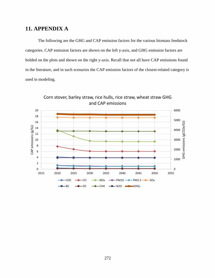
272

11. APPENDIX A

The following are the GHG and CAP emission factors for the various biomass feedstock

categories. CAP emission factors are shown on the left y-axis, and GHG emission factors are

bolded on the plots and shown on the right y-axis. Recall that not all have CAP emissions found

in the literature, and in such scenarios the CAP emission factors of the closest-related category is

used in modeling.

0

1000

2000

3000

4000

5000

6000

0

2

4

6

8

10

12

14

16

18

20

2015 2020 2025 2030 2035 2040 2045 2050 2055

GH

G e

mis

sio

ns

(gC

O2

e/G

J)

CA

P e

mis

sio

ns

(g/G

J)

Corn stover, barley straw, rice hulls, rice straw, wheat straw GHG and CAP emissions

VOC CO NOx PM10 PM2.5 SOx

BC OC CH4 N2O GHGs

273

0

500

1000

1500

2000

0

0.2

0.4

0.6

0.8

1

1.2

2015 2020 2025 2030 2035 2040 2045 2050 2055

GH

G e

mis

sio

ns

(gC

O2

e/G

J)

CA

P e

mis

sio

ns

(g/G

J)Citrus residues, cotton gin trash, cotton residue, noncitrus

residues, tree nut residues GHG and CAP emissions


BC OC CH4 N2O CO2 GHGs

0

500

1000

1500

2000

2500

3000

3500

4000

4500

0

1

2

3

4

5

6

7

8

9

10

2015 2020 2025 2030 2035 2040 2045 2050 2055

GH

G e

mis

sio

ns

CA

P e

mis

sio

ns

(g/G

J)

Miscanthus GHG and CAP emissions



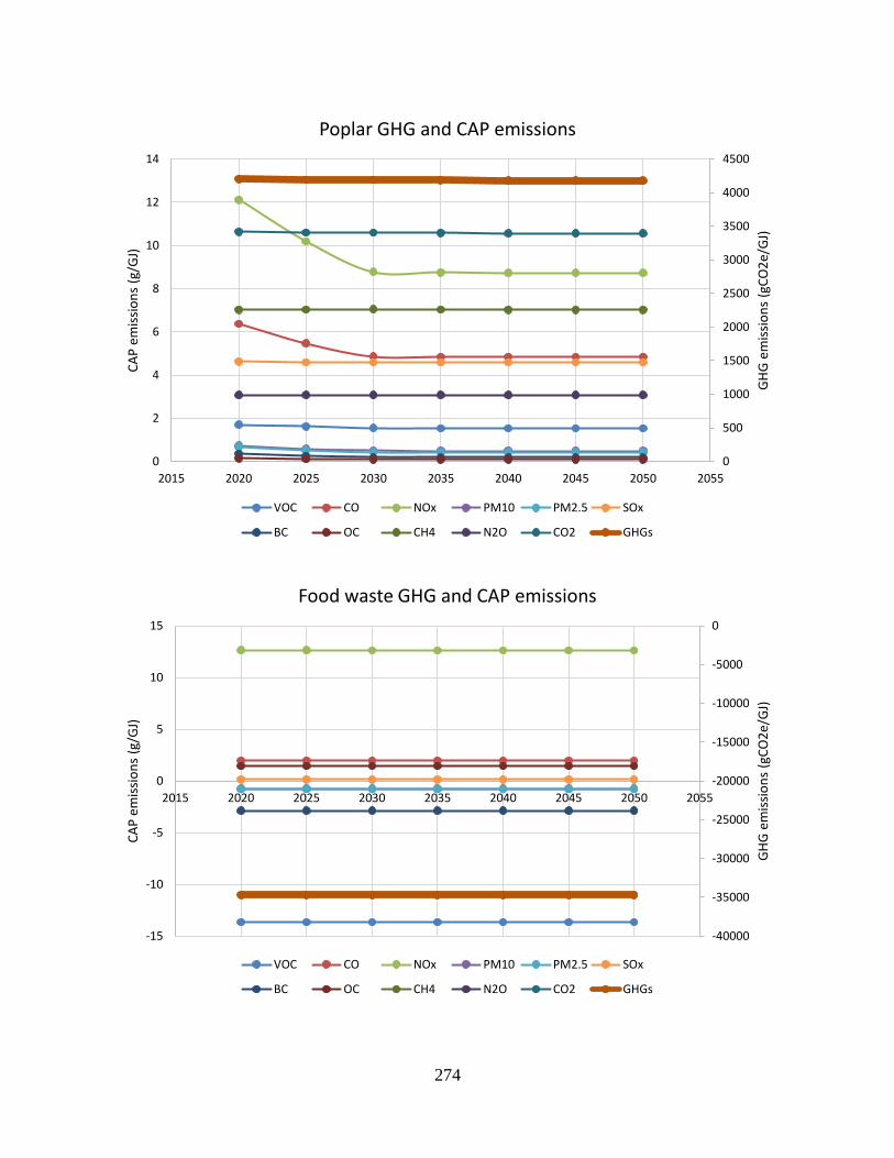
274

0

500

1000

1500

2000

2500

3000

3500

4000

4500

0

2

4

6

8

10

12

14

2015 2020 2025 2030 2035 2040 2045 2050 2055

GH

G e

mis

sio

ns

(gC

O2

e/G

J)

CA

P e

mis

sio

ns

(g/G

J)Poplar GHG and CAP emissions



-40000

-35000

-30000

-25000

-20000

-15000

-10000

-5000

0

-15

-10

-5

0

5

10

15

2015 2020 2025 2030 2035 2040 2045 2050 2055

GH

G e

mis

sio

ns

(gC

O2

e/G

J)

CA

P e

mis

sio

ns

(g/G

J)

Food waste GHG and CAP emissions



275

0

500

1000

1500

2000

2500

3000

0

1

2

3

4

5

6

7

8

9

2015 2020 2025 2030 2035 2040 2045 2050 2055

GH

G e

mis

sio

ns

(gC

O2

e/G

J)

CA

P e

mis

sio

ns

(g/G

J)Hardwood, lowland, residue; hardwood, lowland, tree;

softwood, natural, residue; softwood, natural, tree; softwood, planted, residue; and softwood, planted, tree GHG and CAP

emissions



0

200

400

600

800

1000

1200

1400

1600

1800

2000

0

0.2

0.4

0.6

0.8

1

1.2

2015 2020 2025 2030 2035 2040 2045 2050 2055

GH

G e

mis

sio

ns

(gC

O2

e/G

J)

CA

P e

mis

sio

ns

(g/G

J)

Primary mill residue and Secondary mill residue GHG and CAP emissions



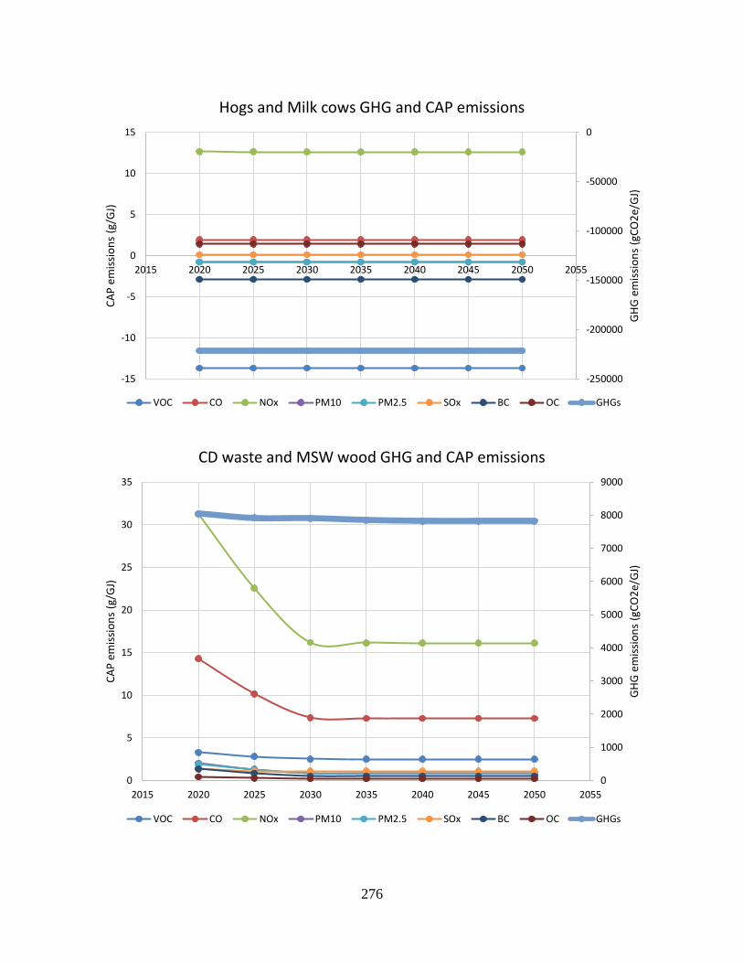
276

-250000

-200000

-150000

-100000

-50000

0

-15

-10

-5

0

5

10

15

2015 2020 2025 2030 2035 2040 2045 2050 2055

GH

G e

mis

sio

ns

(gC

O2

e/G

J)

CA

P e

mis

sio

ns

(g/G

J)Hogs and Milk cows GHG and CAP emissions

VOC CO NOx PM10 PM2.5 SOx BC OC GHGs

0

1000

2000

3000

4000

5000

6000

7000

8000

9000

0

5

10

15

20

25

30

35

2015 2020 2025 2030 2035 2040 2045 2050 2055

GH

G e

mis

sio

ns

(gC

O2

e/G

J)

CA

P e

mis

sio

ns

(g/G

J)

CD waste and MSW wood GHG and CAP emissions

VOC CO NOx PM10 PM2.5 SOx BC OC GHGs

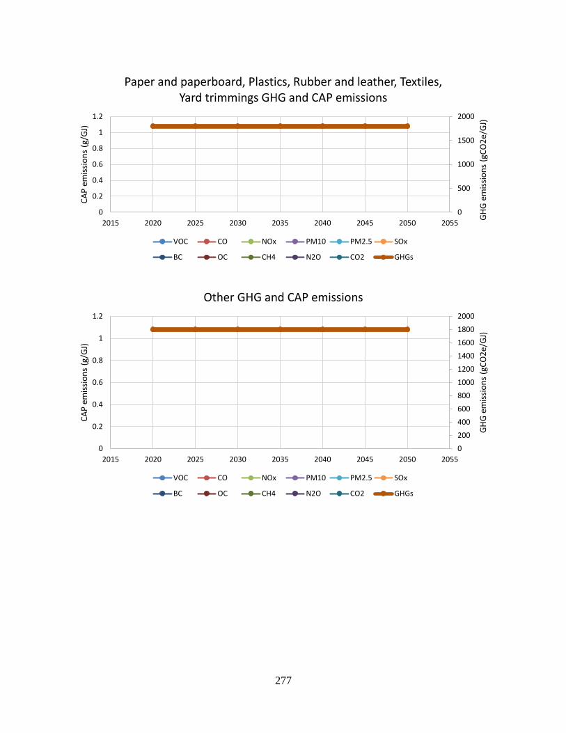
277

0

500

1000

1500

2000

0

0.2

0.4

0.6

0.8

1

1.2

2015 2020 2025 2030 2035 2040 2045 2050 2055

GH

G e

mis

sio

ns

(gC

O2

e/G

J)

CA

P e

mis

sio

ns

(g/G

J)Paper and paperboard, Plastics, Rubber and leather, Textiles,

Yard trimmings GHG and CAP emissions



0

200

400

600

800

1000

1200

1400

1600

1800

2000

0

0.2

0.4

0.6

0.8

1

1.2

2015 2020 2025 2030 2035 2040 2045 2050 2055

GH

G e

mis

sio

ns

(gC

O2

e/G

J)

CA

P e

mis

sio

ns

(g/G

J)

Other GHG and CAP emissions



278

12. APPENDIX B

The following are the vehicle specifications for each of the vehicles modeled, including

LDVs, linehaul HDVs, drayage HDVs, refuse HDVs, and construction HDVs.

Table 34. LDV Specifications

Component ICV HEV PHEV BEV FCEV PFCEV

Glider, LDV (ea.) 1 1 1 1 1 1

ICE, gasoline (kW) 98.43 70.84 70.84

Fuel cell (kW) 114.00 75.00

Traction battery (kwh) 2.16 8.80 60.00 1.60 13.00

Electric motor and inverter (kW) 53.00 53.00 200.00 113.00 112.00

Liquid fuel tank (GJ) 1.74 1.49 1.50

Hydrogen tank (GJ) 0.61 0.48

Hybrid cost, LDV 1 1

Plug-in hybrid cost, LDV 1 1

Table 35. Linehaul HDV Specifications

Component ICV,

diesel

ICV,

SNG

HEV,

diesel

HEV,

SNG

PHEV,

diesel

PHEV,

SNG BEV FCEV PFCEV

Glider,

HDV (ea.) 1 1 1 1 1 1 1 1 1

ICE, diesel

(kW) 324.00 233.18 233.18

ICE, SNG

(kW) 324.00 233.18 233.18

Fuel cell

(kW) 363.00 238.82

Traction

battery

(kwh)

15.00 15.00 88.44 89.58 500.00 2.28 15.72

Electric

motor and

inverter

(kW)

120.00 120.00 120.00 120.00 400.00 400.00 400.00

Liquid fuel

tank (GJ) 12.61 12.61 11.38

SNG tank

(GJ) 15.86 15.86 14.49

Hydrogen

tank (GJ) 10.91 7.33

Hybrid cost,

HDV 1 1 1

Plug-in

hybrid cost,

HDV

1 1 1

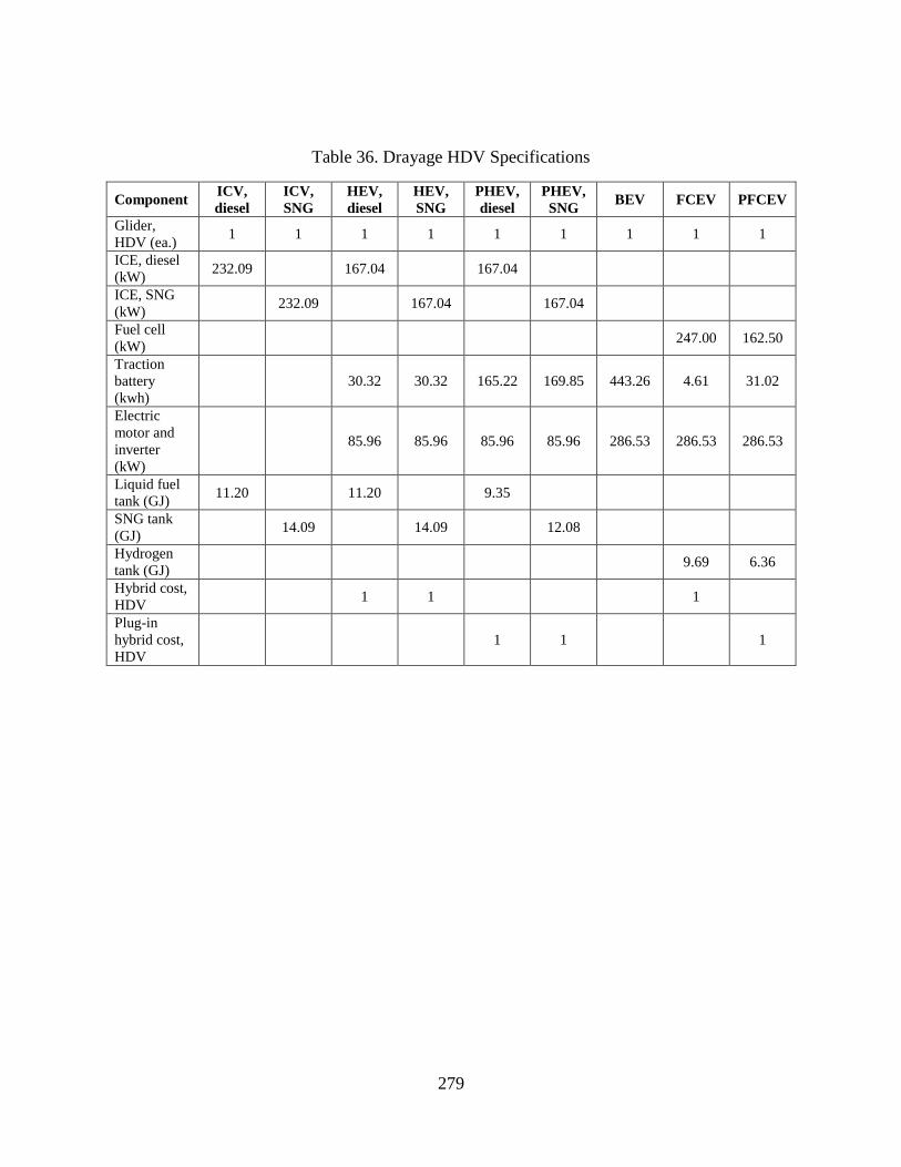
279

Table 36. Drayage HDV Specifications

Component ICV,

diesel

ICV,

SNG

HEV,

diesel

HEV,

SNG

PHEV,

diesel

PHEV,

SNG BEV FCEV PFCEV

Glider,

HDV (ea.) 1 1 1 1 1 1 1 1 1

ICE, diesel

(kW) 232.09 167.04 167.04

ICE, SNG

(kW) 232.09 167.04 167.04

Fuel cell

(kW) 247.00 162.50

Traction

battery

(kwh)

30.32 30.32 165.22 169.85 443.26 4.61 31.02

Electric

motor and

inverter

(kW)

85.96 85.96 85.96 85.96 286.53 286.53 286.53

Liquid fuel

tank (GJ) 11.20 11.20 9.35

SNG tank

(GJ) 14.09 14.09 12.08

Hydrogen

tank (GJ) 9.69 6.36

Hybrid cost,

HDV 1 1 1

Plug-in

hybrid cost,

HDV

1 1 1

280

Table 37. Refuse HDV Specifications

Component ICV,

diesel

ICV,

SNG

HEV,

diesel

HEV,

SNG

PHEV,

diesel

PHEV,

SNG BEV FCEV PFCEV

Glider,

HDV (ea.) 1 1 1 1 1 1 1 1 1

ICE, diesel

(kW) 237.66 171.04 171.04

ICE, SNG

(kW) 237.66 171.04 171.04

Fuel cell

(kW) 273.00 179.61

Traction

battery

(kwh)

30.00 30.00 115.87 123.84 428.57 4.56 25.63

Electric

motor and

inverter

(kW)

88.02 88.02 88.02 88.02 293.41 293.41 293.41

Liquid fuel

tank (GJ) 3.60 3.60 2.13

SNG tank

(GJ) 4.53 4.53 2.86

Hydrogen

tank (GJ) 2.66 1.71

Hybrid cost,

HDV 1 1 1

Plug-in

hybrid cost,

HDV

1 1 1

281

Table 38. Construction HDV Specifications

Component ICV,

diesel

ICV,

SNG

HEV,

diesel

HEV,

SNG

PHEV,

diesel

PHEV,

SNG BEV FCEV PFCEV

Glider,

HDV (ea.) 1 1 1 1 1 1 1 1 1

ICE, diesel

(kW) 172.68 124.27 124.27

ICE, SNG

(kW) 172.68 124.27 124.27

Fuel cell

(kW) 139.00 91.45

Traction

battery

(kwh)

18.19 18.19 85.81 89.04 299.20 2.76 16.62

Electric

motor and

inverter

(kW)

63.95 63.95 63.95 63.95 213.18 213.18 213.18

Liquid fuel

tank (GJ) 5.01 5.01 3.62

SNG tank

(GJ) 6.30 6.30 4.72

Hydrogen

tank (GJ) 3.68 2.54

Hybrid cost,

HDV 1 1 1

Plug-in

hybrid cost,

HDV

1 1 1

Documents

UC Irvine - CORE