Tangent moduli of hot-rolled I-shaped axial members consideringvarious residual stress distributions

Seungjun Kim a, Taek Hee Han b, Deok Hee Won b,c, Young Jong Kang c,n

a Zachry Department of Civil Engineering, Texas A&M University, College Station, TX 77843, USAb Coastal Development & Ocean Energy Research Division, Korea Institute of Ocean Science and Technology, Ansan 426-744, Republic of Koreac School of Architectural, Civil and Environmental Engineering, Korea University, Seoul 136-713, South Korea

a r t i c l e i n f o

Article history:Received 12 March 2013Accepted 15 November 2013Available online 7 December 2013

Keywords:Residual stressTangent modulusHot-rolled sectionPlastic hinge methodInelastic analysis

a b s t r a c t

This paper presents an equation for the effective tangent moduli for steel axial members of hot-rolledI-shaped section subjected to various residual stress distributions. Because of the existence of residualstresses, the cross section yields gradually even when the member is subjected to uniform axial stresses.In the elasto-plastic stage, the structural response can be easily traced using rational tangent modulus ofthe member. In this study, the equations for rational tangent moduli for hot-rolled I-shaped steelmembers in the elasto-plastic stage were derived based on the general principle of force-equilibrium. Forpractical purpose, the equations for the tangent modulus were presented for conventional patterns of theresidual stress distribution of hot-rolled I-shaped steel members. Through a series of material nonlinearanalyses for steel axial members modeled by shell elements, the derived equations were numericallyverified, and the presented equations were compared with the CRC tangent modulus equation, the mostfrequently used equation so far. The comparative study shows that the presented equations areextremely effective for accurately analyzing elasto-plastic behavior of the axially loaded members in asimple manner without using complex shell element models.

& 2013 Elsevier Ltd. All rights reserved.

1. Introduction

In general, hot-rolled steel members are not free from residualstresses distributed in various patterns owing to the characteristicsof the manufacturing method. The existence of residual stressesmay induce gradual yielding in the section of steel members evenwhen external axial loads are applied. To predict the elasto-plasticresponse in the gradual yield stage of the axially loaded steelmembers, the tangent modulus has been widely used for itssimplicity. The CRC (Column Research Council) tangent modulussuggested by Galambos [1] has been the most widely used one. Inparticular, the modulus was used in the plastic hinge method andrefined plastic hinge method to consider gradual yielding of theI-shaped member that has specific residual stress distributions byChen and Lui [2], Liew et al. [3], Chen and Liew [4], Kim and Chen[5], Kim et al. [6], Kim et al. [7], and Kim [8].

But the CRC tangent modulus, which was basically derived viaEuler's elastic buckling equation with assumption of constantmaximum compressive residual stress, has limitations in applic-ability where different various residual stress distributions are tobe considered. As shown in Eq. (1), various effective factors, such

as maximum residual stress values, patterns and the sectionalshapes of members, cannot be considered in the CRC tangentmodulus.

Et ¼ 1:0E Pr0:5Py ð1Þ

Et ¼ 4PPyE 1� P

Py

� �PZ0:5Py ð2Þ

In this study, rational new tangent moduli are derived based onthe general principle of force-equilibrium. First of all, the linearresidual stress distributions suggested by Galambos and Ketter [9],and by ECCS [10], respectively, are considered as the generalresidual stress patterns of hot-rolled steel members. In addition,the parabolic stress distribution suggested by Szali and Papp [11] isalso taken into account. Including the effect of the maximum orminimum residual stress value, the presented equations for thetangent moduli produce clearer and more accurate computation ofthe elasto-plastic behavior. The derived equations are verifiedbased on the results of nonlinear finite element analyses foraxially loaded steel members modeled by shell elements withresidual stress distributions aforementioned. The accuracy and theverification of the presented tangent modulus equations areevidently shown by comparing the load–displacement curvesof nonlinear finite element analyses with those of present study(Fig. 1).

Contents lists available at ScienceDirect

journal homepage: www.elsevier.com/locate/tws

Thin-Walled Structures

0263-8231/$ - see front matter & 2013 Elsevier Ltd. All rights reserved.http://dx.doi.org/10.1016/j.tws.2013.11.005

n Corresponding author. Tel.: þ82 2 3290 3317; fax: þ82 2 921 5166.E-mail address: yjkang@korea.ac.kr (Y.J. Kang).

Thin-Walled Structures 76 (2014) 77–91

2. Residual stresses of hot-rolled I-shaped steel members

Based on the principle of force equilibrium, the resultant forcesin the section of a member that has specific residual stressdistribution should vanish where no external force is applied.As shown in Fig. 2, the residual stress distributions are generallyclassified into two categories, linear and parabolic distributions(Fig. 3).

First of all, the parabolic distribution suggested by Young isbased on an experimental study. Eqs. (3)–(5) show the maximumand minimum residual stresses of the distribution. As shown inthe equations, the residual stress distribution is determined by thesectional dimension parameters, such as height, width and thick-ness of flange and web. Meanwhile, it should be noted thatdifferent steel grades are not taken into account in determiningthe residual stress distribution using the following equations:

f cf ¼ �165 1� htw2:4btf

� �ð3Þ

f cw ¼ �100 1:5� htw2:4btf

� �ð4Þ

f t ¼ 100 0:7� htw2btf

� �ð5Þ

where, fcf and fcw are maximum compressive residual stresses atthe flanges and web, respectively, and ft is the maximum tensileresidual stress at the junctions of the flanges and web; the unitsare N/mm2.

The other parabolic distribution suggested by Szalai and Papp[11] was derived by satisfying all equilibrium equations, includingtorsional and warping effects. As shown in Eqs. (6)–(11), thefunctions of residual stress distribution are determined by thesteel grade as well as by sectional dimension parameters.

f ðyÞ ¼ cf þaf y2 ð6Þ

wðzÞ ¼ cwþawz2 ð7Þ

Nomenclature

A cross-sectional areaAn elastic cross-sectional areab width of flangesE elastic modulusEt tangent modulusΔf additional axial stressfy yield stressf(y) axial stress function at the flanges of the I-shaped

member with parabolic residual stress distributionf(z) axial stress function at the web of the I-shaped

member with parabolic residual stress distributiong coefficient of maximum tensile residual stressh height of a web

h0 net height of a webL length of an axial memberP applied axial forceΔP additional axial forcePt applied total axial forcePy yield axial forcer coefficient of maximum compressive residual stress at

flangesr′ coefficient of maximum compressive residual stress

at a webtf thickness of flangestw thickness of a webυ Poisson's ratioxf length parameter of yield area at flangesxw length parameter of yield area at a web

z

b

h0

tf

twy

h

Fig. 1. Simplified cross section of an I-shaped steel member.

rfy

gfy

gfy

rfy

rfy

rfy

fcf

fcw

ft

f(y)

w(z)

f(y)

Fig. 2. General residual stress distributions: (A) linear (Galambos and Ketter [9]), (B) linear (ECCS [10]) (C) parabolic (Young [12]), and (D) parabolic (Szalai and Papp [11]).

S. Kim et al. / Thin-Walled Structures 76 (2014) 77–9178

where,

cf ¼ αf ybtf ð3b2þ4h2

0Þ2b3tf þ8bh20tf þh3

0twð8Þ

af ¼ �αf y20b3tf þ48bh20tf þ4h30tfb2ð2b3tf þ8bh2

0tf þh30twÞð9Þ

cw ¼ �αf ybtf ð8b3tf þ3b2h0twþ2h30twÞ2h0twð2b3tf þ8bh2

0tf þh30twÞð10Þ

aw ¼ αf y2btf ð8b3tf þ9b2h0twþ10h3

0twÞh30twð2b3tf þ8bh20tf þh30twÞ

ð11Þ

In comparison with parabolic stress distributions, linear stressdistributions are simple to use when considering gradual yield ofthe steel members. For the distribution, the linear distributionssuggested by Galambos and Ketter [9] and ECCS [10] havebeen widely used. In the distribution suggested by Galambos,the maximum tensile residual stress of the web is calculated bythe maximum compressive residual stress of a flange, with thedimension of the section as follows:

f w ¼ � btf f c1ðbtf þhtwÞ

ð12Þ

As shown in Fig. 2(B), the distribution suggested by ECCS [10] issimplest among the distributions introduced in the figure. Theabsolute value of maximum and minimum residual stress of flangeand web are exactly the same. So, the force equilibrium condition,which means that all resultant forces should be zero when noexternal forces are applied, is automatically satisfied.

In this study, the previously mentioned residual stress distribu-tions are considered for wide applicability of the derived tangentmodulus, except for the parabolic distribution suggested by Young[12], because of its limitation of not considering steel grades.In other words, individual equations of effective tangent modulusfor members that have the linear and parabolic stress distributionssuggested by Galambos and Ketter [9], ECCS [10] and Szalai andPapp [11], are derived and suggested.

3. Equations of tangent moduli that consider linear residualstress distributions

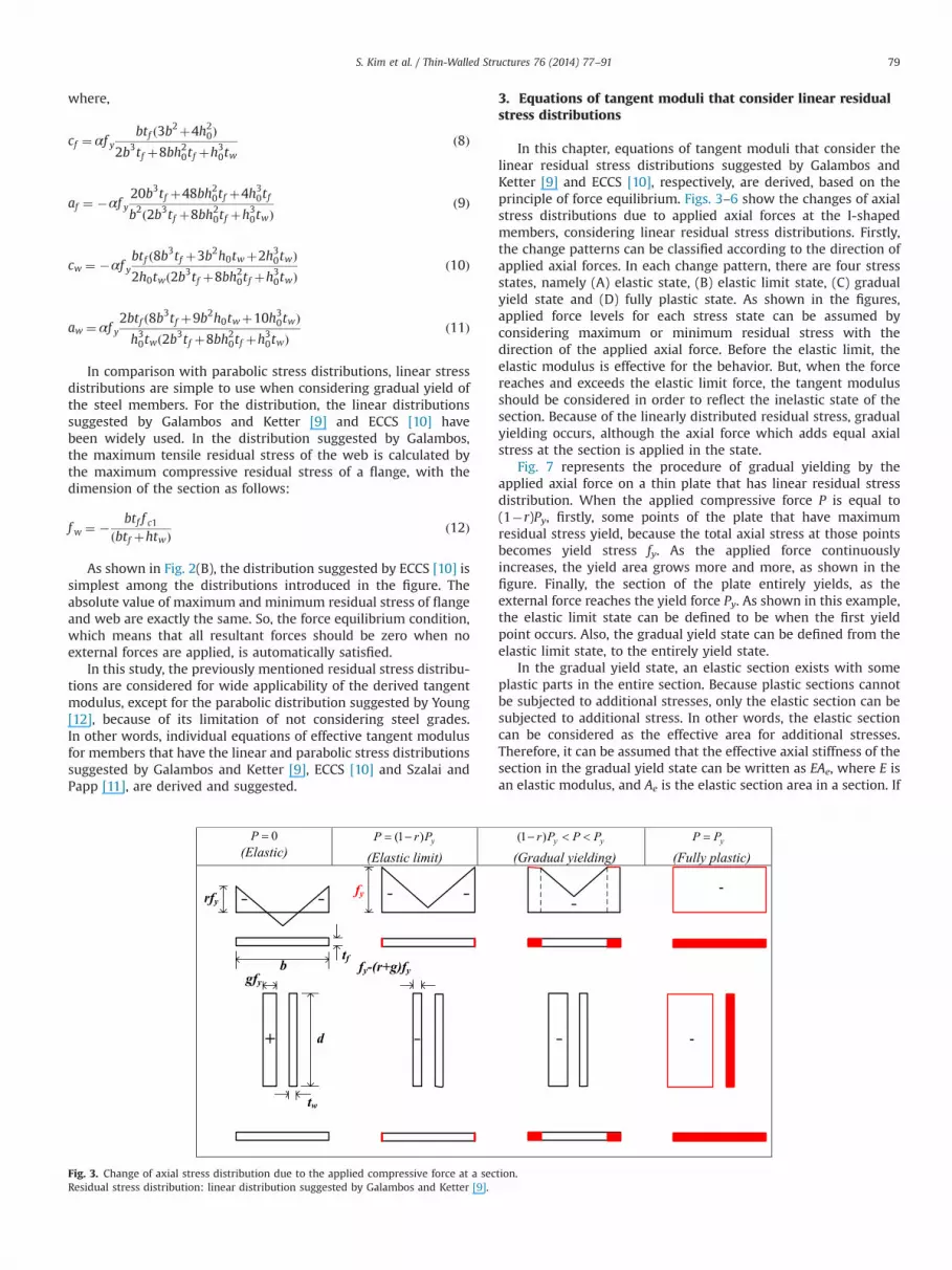
In this chapter, equations of tangent moduli that consider thelinear residual stress distributions suggested by Galambos andKetter [9] and ECCS [10], respectively, are derived, based on theprinciple of force equilibrium. Figs. 3–6 show the changes of axialstress distributions due to applied axial forces at the I-shapedmembers, considering linear residual stress distributions. Firstly,the change patterns can be classified according to the direction ofapplied axial forces. In each change pattern, there are four stressstates, namely (A) elastic state, (B) elastic limit state, (C) gradualyield state and (D) fully plastic state. As shown in the figures,applied force levels for each stress state can be assumed byconsidering maximum or minimum residual stress with thedirection of the applied axial force. Before the elastic limit, theelastic modulus is effective for the behavior. But, when the forcereaches and exceeds the elastic limit force, the tangent modulusshould be considered in order to reflect the inelastic state of thesection. Because of the linearly distributed residual stress, gradualyielding occurs, although the axial force which adds equal axialstress at the section is applied in the state.

Fig. 7 represents the procedure of gradual yielding by theapplied axial force on a thin plate that has linear residual stressdistribution. When the applied compressive force P is equal to(1�r)Py, firstly, some points of the plate that have maximumresidual stress yield, because the total axial stress at those pointsbecomes yield stress fy. As the applied force continuouslyincreases, the yield area grows more and more, as shown in thefigure. Finally, the section of the plate entirely yields, as theexternal force reaches the yield force Py. As shown in this example,the elastic limit state can be defined to be when the first yieldpoint occurs. Also, the gradual yield state can be defined from theelastic limit state, to the entirely yield state.

In the gradual yield state, an elastic section exists with someplastic parts in the entire section. Because plastic sections cannotbe subjected to additional stresses, only the elastic section can besubjected to additional stress. In other words, the elastic sectioncan be considered as the effective area for additional stresses.Therefore, it can be assumed that the effective axial stiffness of thesection in the gradual yield state can be written as EAe, where E isan elastic modulus, and Ae is the elastic section area in a section. If

Fig. 3. Change of axial stress distribution due to the applied compressive force at a section.Residual stress distribution: linear distribution suggested by Galambos and Ketter [9].

S. Kim et al. / Thin-Walled Structures 76 (2014) 77–91 79

the elastic sectional area Ae in the gradual yield state can becalculated, the tangent modulus can be calculated by the followingrelationship:

EAe ¼ EtA ð13Þ

The elastic sectional area Ae can be calculated using therelationship between the increased axial force ΔP from the elasticlimit state, increased axial stressΔf due to the increased force, andthe length of yield sectional parts due to the stress increasing. Inthe next paragraphs, the equations of tangent moduli consideringlinear residual stress distributions are derived by the assumptionand relationships mentioned previously.

3.1. Tangent moduli considering the linear residual stressdistribution suggested by Galambos and Ketter [9]

Fig. 8 shows the stress distribution in the gradual yield stateat a section that has the linear residual stress distributionsuggested by Galambos and Ketter [9]. In the figure, Δf is theadditional axial stress induced by additional axial force ΔPfrom an elastic limit state. As shown in the figure, stressdistributions can be assumed according to the direction ofapplied forces.

The tangent modulus for the applied compressive forcecan be derived as follows. First, the length of yield area xfshown in the figure can be derived by the following

Fig. 5. Change of axial stress distribution due to the applied compressive force at a section.Residual stress distribution: linear distribution suggested by ECCS [10].

Fig. 4. Change of axial stress distribution due to the applied tensile force at a section.Residual stress distribution: linear distribution suggested by Galabos and Ketter [9].

S. Kim et al. / Thin-Walled Structures 76 (2014) 77–9180

relationship:

ðrþgÞf y :b2¼Δf : xf ð14Þ

xf ¼Δf b

2ðrþgÞf y¼ bðbtf þh0twÞ

2rAΔff y

ð15Þ

where g¼ ðrbtf Þ=ðbtf þh0twÞ.

The total applied axial force Pt at the section can be calculatedby integration of the axial stress via the sectional area as follows:

Pt ¼ZAf dA¼ 2Δf btf þ2f ybtf �ðrþgÞf ybtf �2Δf xf tf þΔf h0tw

þ½1�ðrþgÞ�hskip2ptf yh0tw ð16Þ

also, the force can be written as follows:

Pt ¼ ð1�rÞPyþΔP ð17Þ

Fig. 7. Gradual yield induced by the applied axial force on a plate that has linear residual stress distribution (applied axial force: compressive).

Fig. 8. Stress distribution in gradual yield states (Δf: additional axial stress due to additional applied force ΔP from the elastic limit).

Fig. 6. Change of axial stress distribution due to the applied tensile force at a section.Residual stress distribution: linear distribution suggested by ECCS [10].

S. Kim et al. / Thin-Walled Structures 76 (2014) 77–91 81

where ΔP is the additional axial force applied after the elasticlimit state.

Substituting Eq. (15) into the xf in Eq. (16), additional stress theΔf induced by an additional force ΔP can be calculated as follows:

Δf ¼K�

ffiffiffiffiffiffiffiffiffiffiffiffiffiffiffiffiffiffiffiffiffiffiffiffiffiffiffiffiffiffiffiffiffiffiffiffiffiffiffiffiffiffiffiffiffiffiK2�4K½Pt�ð1�rÞPy�

q2A

ð18Þ

where K ¼ A2rPy=ðbtf ðbtf þh0twÞÞ.So, the length of yield area at the flange can be calculated using

additional stress Δf and Eq. (15), as follows:

xf ¼ bK�

ffiffiffiffiffiffiffiffiffiffiffiffiffiffiffiffiffiffiffiffiffiffiffiffiffiffiffiffiffiffiffiffiffiffiffiffiffiffiffiffiffiffiffiffiffiffiK2�4K½Pt�ð1�rÞPy�

q4ðrþgÞPy

ð19Þ

where ð1�rÞPyrPtrPy.Using the length xf, the elastic area An can be easily calculated,

and the tangent elastic modulus can be obtained by the equationof the stiffness of axial members as follows:

AnE¼ ½A�ð4xf tf Þ�E¼ AEt ð20Þ

‘Et ¼ 1�ð4xf tf ÞA

� �E ð21Þ

Finally, the tangent modulus can be summarized as follows:

Et ¼ E 0rPtoð1�rÞPy ð22Þ

Et ¼ 1�ð4xf tf ÞA

� �E ð1�rÞPyrPtrPy ð23Þ

where,

xf ¼ bK�

ffiffiffiffiffiffiffiffiffiffiffiffiffiffiffiffiffiffiffiffiffiffiffiffiffiffiffiffiffiffiffiffiffiffiffiffiffiffiffiffiffiffiffiffiffiffiK2�4K½Pt�ð1�rÞPy�

q4ðrþgÞPy

K ¼ A2rPy

btf ðbtf þh0twÞ

The tangent moduli for I-shaped members subjected to tensileforces can be derived via the same way. Using the stress distribu-tion shown in Fig. 8, the length parameter of yield area xf at theflanges can be calculated using the rule of proportional relation-ship shown in the figure.

ðrþgÞf y :b2¼Δf : xf ð24Þ

xf ¼b2

ΔfðrþgÞf y

¼ bðbtf þh0twÞ2rA

Δff y

ð25Þ

Also, the total force Pt can be calculated by integration of thestress distribution via the entire sectional area, as follows:

Pt ¼ZAf dA¼ 2Δf btf þ2f ybtf �ðrþgÞf ybtf �

btfðrþgÞ

Δf 2

f yþ f yh0tw ¼ ð1�gÞPyþΔP ð26Þ

Substituting Eq. (25) into the xf in Eq. (26), the additional stressΔf induced by an additional force ΔP can be calculated as follows:

Δf ¼ðrþgÞPy�

ffiffiffiffiffiffiffiffiffiffiffiffiffiffiffiffiffiffiffiffiffiffiffiffiffiffiffiffiffiffiffiffiffiffiffiffiffiffiffiffiffiffiffiffiffiffiffiffiffiffiffiffiffiffiffiffiffiffiffiffi½ðrþgÞPy�2�K½Pt�ð1�gÞPy�

qA

ð27Þ

where, K ¼ A2rPy=ðbtf ðbtf þh0twÞÞThus, the length of yield area at flanges x can be calculated as

follows:

xf ¼ bUðrþgÞPy�

ffiffiffiffiffiffiffiffiffiffiffiffiffiffiffiffiffiffiffiffiffiffiffiffiffiffiffiffiffiffiffiffiffiffiffiffiffiffiffiffiffiffiffiffiffiffiffiffiffiffiffiffiffiffiffiffiffiffiffiffi½ðrþgÞPy�2�K½Pt�ð1�gÞPy�

q2ðrþgÞPy

ð28Þ

Using the effective axial stiffness in a gradual yield statewritten as follows, the tangent modulus can be calculated as

shown in Eq. (30).

AnE¼ ½A�ð4xf tf þh0twÞ�E¼ AEt ð29Þ

‘Et ¼ 1�ð4xf tf þh0twÞA

� �E ð30Þ

Finally, the tangent modulus can be summarized as follows:

Et ¼ E 0rPto ð1�gÞPy ð31Þ

Et ¼ 1�ð4xf tf þh0twÞA

� �E ð1�gÞPyrPtrPy ð32Þ

where,

xf ¼ bðrþgÞPy�

ffiffiffiffiffiffiffiffiffiffiffiffiffiffiffiffiffiffiffiffiffiffiffiffiffiffiffiffiffiffiffiffiffiffiffiffiffiffiffiffiffiffiffiffiffiffiffiffiffiffiffiffiffiffiffiffiffiffiffiffi½ðrþgÞPy�2�K½Pt�ð1�gÞPy�

q2ðrþgÞPy

K ¼ A2rPy

btf ðbtf þh0twÞ

3.2. Tangent moduli considering the linear residual stressdistribution suggested by ECCS [10]

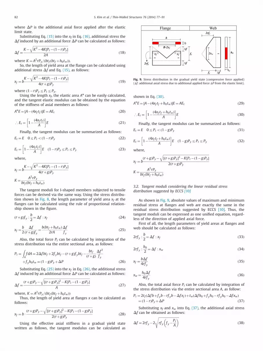
As shown in Fig. 9, absolute values of maximum and minimumresidual stress at flanges and web are exactly the same in theresidual stress distribution suggested by ECCS [10]. Thus, thetangent moduli can be expressed as one unified equation, regard-less of the direction of applied axial force.

First of all, the length parameters of yield areas at flanges andweb should be calculated as follows:

2rf y :b2¼Δf : xf ð33Þ

2rf y :h0

2¼Δf : xw ð34Þ

xf ¼bΔf4rf y

ð35Þ

xw ¼ h0Δf4rf y

ð36Þ

Also, the total axial force Pt can be calculated by integration ofthe stress distribution via the entire sectional area A, as follow:

Pt ¼ 2tf ðΔf bþ f yb�rf yb�Δf xf ÞþtwðΔf h0þ f yh0�rf yh0�Δf xwÞ¼ ð1�rÞPyþΔP ð37ÞSubstituting xf and xw into Eq. (37), the additional axial stress

Δf can be obtained as follows:

Δf ¼ 2rf y�2

ffiffiffiffiffiffiffiffiffiffiffiffiffiffiffiffiffiffiffiffiffiffiffiffiffiffiffirf y f y�

Pt

A

� �sð38Þ

Fig. 9. Stress distribution in the gradual yield state (compressive force applied)(Δf: additional axial stress due to additional applied force ΔP from the elastic limit).

S. Kim et al. / Thin-Walled Structures 76 (2014) 77–9182

So, xf and xw can be summarized by substituting the equationfor Δf into Eqs. (35) and (36), respectively.

xf ¼ brPy�

ffiffiffiffiffiffiffiffiffiffiffiffiffiffiffiffiffiffiffiffiffiffiffiffirPyðPy�PtÞ

p2rPy

ð39Þ

xw ¼ h0rPy�

ffiffiffiffiffiffiffiffiffiffiffiffiffiffiffiffiffiffiffiffiffiffiffiffirPyðPy�PtÞ

p2rPy

ð40Þ

Using the effective axial stiffness in the gradual yield statewritten as follows, the tangent modulus can be calculated asshown in Eq. (42).

AnE¼ ½A�ð4xf tf þ2xwtwÞ�E¼ AEt ð41Þ

‘Et ¼ 1�ð4xf tf þ2xwtwÞA

� �E ð42Þ

Finally, the tangent modulus can be summarized as follows:

Et ¼ E 0rPto ð1�rÞPy ð43Þ

Et ¼ 1�ð4xf tf þ2xwtwÞA

� �E ð1�rÞPyrPtrPy ð44Þ

where,

xf ¼ brPy�

ffiffiffiffiffiffiffiffiffiffiffiffiffiffiffiffiffiffiffiffiffiffiffiffirPyðPy�PtÞ

p2rPy

xw ¼ h0rPy�

ffiffiffiffiffiffiffiffiffiffiffiffiffiffiffiffiffiffiffiffiffiffiffiffirPyðPy�PtÞ

p2rPy

4. Equation of tangent moduli that consider a parabolicresidual stress distribution

In the present section, equations of tangent moduli for theparabolic residual stress distribution suggested by Szali and Papp[11] are derived based on the principle of force-equilibrium. Fig. 10shows the change of stress distributions with respect to theapplied axial force level. When compressive force is applied, theprocedure of stress distribution changes can be divided into twocategories, because the maximum compressive residual stresses atflange and web are different from each other. For example, if themaximum compressive residual stress of the flange is greater thanthat of the web, the flange will yield prior to the web when thesame axial stress is added by an applied compressive force. As theapplied force increases, the web also begins to yield; and finally,both flanges and web yield entirely when the applied forcereaches the yield force Py. On the other hand, when the maximumcompressive residual stress of the web is greater than that of the

Fig. 10. Change of the axial stress distribution due to the applied compressive force at the section.Residual stress distribution: parabolic distribution suggested by Szali and Papp [11].

S. Kim et al. / Thin-Walled Structures 76 (2014) 77–91 83

flange, the first yield occurs at the web. This implies that theequations of tangent moduli should be considered differently byrecognizing the difference in gradual yielding procedures whenthe parabolic residual stress distribution is considered. As shownin the figure, in this study, the two cases are considered separatelyto clearly derive the tangent moduli for the parabolic residualstress distribution. On the other hand, the tangent modulus whentensile force is applied is not divided into two cases, because themaximum tensile residual stresses at the flange and web areassumed to have exactly the same value. Thus, the first yielding offlange and web begin at the same time. Consequently, the stressstates of a member, when tensile force is applied, can be classifiedas follows: (A) elastic state, (B) elastic limit state, (C) gradual yieldstate (at entire section), and (D) fully plastic state.

4.1. Tangent modulus for Case 1

When the maximum compressive residual stress of the flangeis greater than that of the web, gradual yield would start at theflange first. In this state, the web maintains an elastic state, whilethe flange suffers gradual yielding. As the applied compressiveforce further increases, the web also suffers gradual yielding.Consequently, the inelastic path from elastic limit to full plasticstate can be divided into two steps: the first is the flange gradualyield state, and the second is the flange/web gradual yield state. Toderive accurate tangent moduli, the equations for the moduli arederived with respect to the sequential steps.

4.1.1. Tangent modulus in the flange gradual yield stepFirstly, the stress distribution at the elastic limit state can be

expressed using the residual stress distribution functions, asfollows:

f ðyÞ ¼ af y2þcf þð1�rÞf y ð45Þ

f ðzÞ ¼ awz2þcwþð1�rÞf y ð46Þ

where, f(y) is the stress distribution of the flanges, and f(z) is thestress distribution of the web.

Also, af, cf, aw and cw are coefficients presented by the parabolicresidual stress distribution suggested by Szali and Papp, as shownin Eqs. (8)–(11).

After that, as the additional axial stress Δf induced by theadditional compressive forceΔP from the elastic state is applied tothe section, the stress distribution changes, as follows:

f ðyÞ ¼ af y2þcf þð1�rÞf yþΔf �ðb=2�xf Þryrðb=2�xf Þ ð47Þ

f ðyÞ ¼ f y yr�ðb=2�xf Þ; yZ ðb=2�xf Þ ð48Þ

f ðzÞ ¼ awz2þcwþð1�rÞf yþΔf �h0=2rzrh0=2 ð49Þ

In Eq. (47), the stress resultant at y¼(b/2)�xf should be theyield stress fy. So, the length of yield section at the flange can beobtained by substituting y¼(b/2)�xf into Eq. (47) as follows:

xf ¼af b�

ffiffiffiffiffiffiffiffiffiffiffiffiffiffiffiffiffiffiffiffiffiffiffiffiffiffiffiffiffiffiffiffiffiffiffiffiffi4af ðrf y�cf �Δf Þ

q2af

ð50Þ

The total applied compressive force Pt can be expressed in thefollowing form:

Pt ¼ 4tf

Z b=2�xf

0½af y2þcf þð1�rÞf yþΔf �dyþ2tw

Z h0=2

0½awz2

þcwþð1�rÞf yþΔf �dwþ4xf tf f y ¼ ð1�rÞPyþΔP ð51Þ

In Eqs. (50) and (51), xf and Δf are unknown values when atotal force Pt is applied in the gradual yield state. Thus, the

unknown values can be obtained by solving the simultaneousequations of Eqs. (50) and (51).

After obtaining xf, the elastic area An can be calculated, asfollows:

An ¼ A�4xf tf ð52Þ

Using the axial stiffness equation, the tangent modulus in thestate can be estimated, as follows:

Et ¼ 1�ð4xf tf ÞA

� �E ð1�rÞPyrPto ð1�r′ÞPy ð53Þ

where xf can be obtained by solving the simultaneous equations ofEqs. (50) and (51).

4.1.2. Tangent moduli in the flange/web gradual yield stepWhen the flanges and web suffer gradual yielding together, the

stress distribution functions can be expressed as follows:

f ðyÞ ¼ af y2þcf þð1�rÞf yþΔf �ðb=2�xf Þryr ðb=2�xf Þ ð54Þ

f ðyÞ ¼ f y yr�ðb=2�xf Þ; yZðb=2�xf Þ ð55Þ

f ðzÞ ¼ awz2þcwþð1�rÞf yþΔf zr�xw; zZxw ð56Þ

f ðzÞ ¼ f y �xwrzrxw ð57Þ

The length parameters of yield area at the flange and web, xfand xw can be calculated using the following relationships:

f ðb=2�xf Þ ¼ af ðb=2�xf Þ2þcf þð1�rÞf yþΔf ¼ f y ð58Þ

f ðxwÞ ¼ awðxwÞ2þcwþð1�rÞf yþΔf ¼ f y ð59Þ

Thus, the parameters can be expressed as follows:

xf ¼af b�

ffiffiffiffiffiffiffiffiffiffiffiffiffiffiffiffiffiffiffiffiffiffiffiffiffiffiffiffiffiffiffiffiffiffiffiffiffi4af ðrf y�cf �Δf Þ

q2af

ð60Þ

xw ¼ffiffiffiffiffiffiffiffiffiffiffiffiffiffiffiffiffiffiffiffiffiffiffiffiffiffiffiffiffiffiffiffi�cw�rf yþΔf

aw

sð61Þ

The total applied compressive force Pt can be expressed in thefollowing form:

Pt ¼ 4tf

Z b=2�xf

0½af y2þcf þð1�rÞf yþΔf �dyþ2tw

Z h0=2

xw½awz2þcw

þð1�rÞf yþΔf �dwþ4xf tf f yþ2xwtwf y ð62Þ

In the gradual yield state, the elastic area An can be calculated ifthe lengths of yield area at flanges and web are obtained asfollows:

An ¼ A�4xf tf �2xwtw ð63Þ

Thus, the tangent modulus can be expressed as follows:

‘Et ¼ 1�ð4xf tf þ2xwtwÞA

� �E ð1�r′ÞPyoPtrPy ð64Þ

where xf and xw can be obtained by solving the simultaneousequations of Eqs. (60)–(62).

4.2. Tangent moduli for Case 2

Because of the characteristics of parabolic residual stressdistribution, the maximum compressive residual stress of theweb might be greater than that of the flange, according to thegeometry of the section. In the following paragraphs, the tangentmoduli for Case 2 introduced previously are derived.

S. Kim et al. / Thin-Walled Structures 76 (2014) 77–9184

4.2.1. Tangent moduli in the web gradual yield stepFirst of all, the stress distribution at the elastic limit state can be

expressed using the residual stress distribution functions, asfollows:

f ðyÞ ¼ af y2þcf þð1�r′Þf y ð65Þ

f ðzÞ ¼ awz2þcwþð1�r′Þf y ð66ÞAfter that, as additional axial stressΔf is applied to the section,

the stress distribution changes as follows:

f ðyÞ ¼ af y2þcf þð1�r′Þf yþΔf �b=2ryrb=2 ð67Þ

f ðzÞ ¼ awz2þcwþð1�r′Þf yþΔf zr�xw; zZxw ð68Þ

f ðzÞ ¼ f y �xwrzrxw ð69ÞIn Eq. (68), the stress resultant at z¼xw should be the yield

stress. So, the length of yield at the flange can be obtained bysubstituting z¼xw into the equation, as follows:

xw ¼ffiffiffiffiffiffiffiffiffiffiffiffiffiffiffiffiffiffiffiffiffiffiffiffiffiffiffiffiffiffiffiffiffiffi�cw�r′f yþΔf

aw

sð70Þ

The total applied compressive force Pt can be expressed in thefollowing form:

Pt ¼ 4tf

Z b=2

0af y

2þcf þð1�r′Þf yþΔf� �

dyþ2twZ h0=2

xw½awz2

þcwþð1�r′Þf yþΔf �dwþ2xwtwf y ¼ ð1�r′ÞPyþΔP ð71Þ

An area An in the elastic state can be calculated as follows:

An ¼ A�2xwtw ð72ÞThus, the tangent modulus equation can be expressed as

follows:

Et ¼ 1�ð2xwtwÞA

� �E ð1�r′ÞPyrPto ð1�rÞPy ð73Þ

where xw can be obtained by solving the simultaneous equationsof Eqs. (70) and (71).

4.2.2. Flange and web: gradual yield stateBasically, the tangent moduli equation for this state can also be

derived with the same procedure introduced in Section 4.1.2. Thus,the tangent moduli for the state in Case 2 can be expressed asfollows:

‘Et ¼ 1�ð4xf tf þ2xwtwÞA

� �E ð1�rÞPyoPtrPy ð74Þ

where xf and xw can be obtained by solving the simultaneousequations of Eqs. (60)–(62) as introduced in Section 4.1.2.

The equations of tangent moduli for parabolic residual stressdistribution show more complex forms than those for linearresidual stress distribution. Because of the characteristics of stress

distribution, the equations should be considered with individualsteps in different cases, as shown in this chapter. Also, there isdifficulty in simplifying the equations of tangent moduli comparedwith the equations for the linear stress distributions. As shown inthis chapter, the length parameters of yield parts should beobtained by solving simultaneous equations that consist of variousterms. But the simultaneous equations can be easily solved, usinggeneral mathematic programs, such as Mathlab and Mathcad.

5. Verification of the suggested equations for the tangentmoduli that consider linear residual stress distributions

To verify the derived equations for the tangent moduli, non-linear analyses are performed, using I-shaped axial membersmodeled by 4 node shell elements. Verification for the derivedequations is performed by comparing the analysis results with thecalculated load–displacement curves obtained by the CRC tangentmodulus and the suggested modulus, respectively. For nonlinearanalysis, ABAQUS V6.10 [13] is used. Also, the initial conditionoption presented by ABAQUS V6.10 [13] is used to define theresidual stress distributions before nonlinear analysis, under thedefined axial force condition.

5.1. Analysis model

For verification of the suggested equations for the tangentmoduli, 3.0 m long I-shaped plate axial members are used. InTable 1, the sectional properties of the members are representedwith material properties. Also, an elastic-perfect plastic materialmodel is assumed as the stress–strain relationship– of the steelmodel (Tables 2–7).

To model the axial member, one of the ends of the member isconsidered as a fixed boundary, while the other end is subjected toaxial force, as shown in Fig. 11. In the fixed end, axial displacementis restricted at every node in the section. Also, lateral displace-ments are restricted at the two joints between the flanges with theweb and the center node of the web, while torsional rotation isrestricted at the center node of the web. In this analytical verifi-cation, 0.3 and 0.5 are considered as r, the maximum compressiveresidual stress constant.

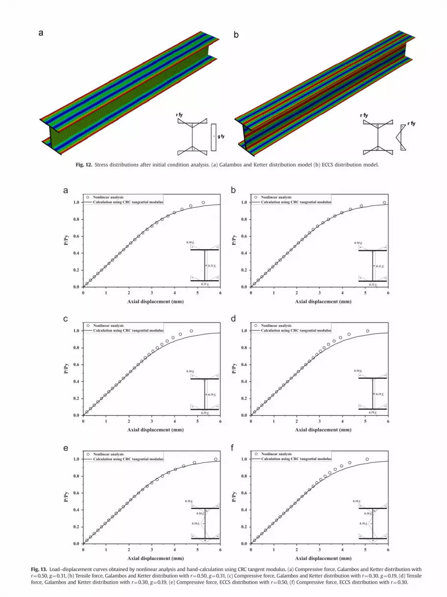
Nonlinear analysis for the member subjected to axially loadedforce is performed after the initial condition analysis, to considerthe residual stress distribution. Fig. 12 shows the stress distribu-tions after the initial condition analysis, and shows the pre-defined residual stress distributions well.

5.2. Comparison of load–displacement curves obtained by nonlinearanalysis and CRC tangent modulus.

In these paragraphs, the applicability of the CRC tangentmodulus, formerly a well-used equation, is briefly studied, basedon the results of nonlinear finite element analysis. For the study,the load–displacement curves at the center of the loading sectionare compared with each other. As shown in Fig. 13, there aredifferences between the load–displacement curves obtained bynonlinear analysis and hand-calculation using CRC tangent mod-ulus equations, respectively. As the load increase more and more,the difference in the paths of both curves also grows more andmore. This originates from the limitation of the consideration ofthe maximum residual stress constants, stress distribution, dimen-sions of the section, and loading direction. Using the CRC tangentmodulus equation, these factors cannot be considered. Therefore,inaccurate results could be obtained when the tangent modulus isused to obtain the structural response in a gradual yield state of anI-shaped member with specific residual stress distributions.

Table 1Geometric and material properties of analysis models.

E (MPa) 2.1� 105

b (mm) 300.0h (mm) 300.0tf, tw(mm) 15.0, 10.0fy (MPa) 280.0υ 0.3r 0.5, 0.3

S. Kim et al. / Thin-Walled Structures 76 (2014) 77–91 85

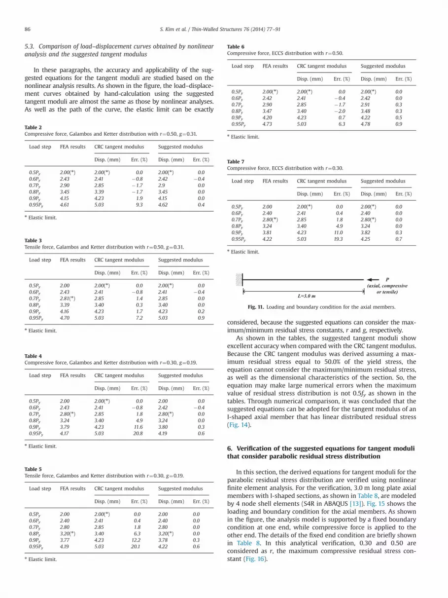
5.3. Comparison of load–displacement curves obtained by nonlinearanalysis and the suggested tangent modulus

In these paragraphs, the accuracy and applicability of the sug-gested equations for the tangent moduli are studied based on thenonlinear analysis results. As shown in the figure, the load–displace-ment curves obtained by hand-calculation using the suggestedtangent moduli are almost the same as those by nonlinear analyses.As well as the path of the curve, the elastic limit can be exactly

considered, because the suggested equations can consider the max-imum/minimum residual stress constants, r and g, respectively.

As shown in the tables, the suggested tangent moduli showexcellent accuracy when compared with the CRC tangent modulus.Because the CRC tangent modulus was derived assuming a max-imum residual stress equal to 50.0% of the yield stress, theequation cannot consider the maximum/minimum residual stress,as well as the dimensional characteristics of the section. So, theequation may make large numerical errors when the maximumvalue of residual stress distribution is not 0.5fy as shown in thetables. Through numerical comparison, it was concluded that thesuggested equations can be adopted for the tangent modulus of anI-shaped axial member that has linear distributed residual stress(Fig. 14).

6. Verification of the suggested equations for tangent modulithat consider parabolic residual stress distribution

In this section, the derived equations for tangent moduli for theparabolic residual stress distribution are verified using nonlinearfinite element analysis. For the verification, 3.0 m long plate axialmembers with I-shaped sections, as shown in Table 8, are modeledby 4 node shell elements (S4R in ABAQUS [13]). Fig. 15 shows theloading and boundary condition for the axial members. As shownin the figure, the analysis model is supported by a fixed boundarycondition at one end, while compressive force is applied to theother end. The details of the fixed end condition are briefly shownin Table 8. In this analytical verification, 0.30 and 0.50 areconsidered as r, the maximum compressive residual stress con-stant (Fig. 16).

Table 2Compressive force, Galambos and Ketter distribution with r¼0.50, g¼0.31.

Load step FEA results CRC tangent modulus Suggested modulus

Disp. (mm) Err. (%) Disp. (mm) Err. (%)

0.5Py 2.00(n) 2.00(n) 0.0 2.00(n) 0.00.6Py 2.43 2.41 �0.8 2.42 �0.40.7Py 2.90 2.85 �1.7 2.9 0.00.8Py 3.45 3.39 �1.7 3.45 0.00.9Py 4.15 4.23 1.9 4.15 0.00.95Py 4.61 5.03 9.3 4.62 0.4

n Elastic limit.

Table 3Tensile force, Galambos and Ketter distribution with r¼0.50, g¼0.31.

Load step FEA results CRC tangent modulus Suggested modulus

Disp. (mm) Err. (%) Disp. (mm) Err. (%)

0.5Py 2.00 2.00(n) 0.0 2.00(n) 0.00.6Py 2.43 2.41 �0.8 2.41 �0.40.7Py 2.81(n) 2.85 1.4 2.85 0.00.8Py 3.39 3.40 0.3 3.40 0.00.9Py 4.16 4.23 1.7 4.23 0.20.95Py 4.70 5.03 7.2 5.03 0.9

n Elastic limit.

Table 4Compressive force, Galambos and Ketter distribution with r¼0.30, g¼0.19.

Load step FEA results CRC tangent modulus Suggested modulus

Disp. (mm) Err. (%) Disp. (mm) Err. (%)

0.5Py 2.00 2.00(n) 0.0 2.00 0.00.6Py 2.43 2.41 �0.8 2.42 �0.40.7Py 2.80(n) 2.85 1.8 2.80(n) 0.00.8Py 3.24 3.40 4.9 3.24 0.00.9Py 3.79 4.23 11.6 3.80 0.30.95Py 4.17 5.03 20.8 4.19 0.6

n Elastic limit.

Table 5Tensile force, Galambos and Ketter distribution with r¼0.30, g¼0.19.

Load step FEA results CRC tangent modulus Suggested modulus

Disp. (mm) Err. (%) Disp. (mm) Err. (%)

0.5Py 2.00 2.00(n) 0.0 2.00 0.00.6Py 2.40 2.41 0.4 2.40 0.00.7Py 2.80 2.85 1.8 2.80 0.00.8Py 3.20(n) 3.40 6.3 3.20(n) 0.00.9Py 3.77 4.23 12.2 3.78 0.30.95Py 4.19 5.03 20.1 4.22 0.6

n Elastic limit.

Table 6Compressive force, ECCS distribution with r¼0.50.

Load step FEA results CRC tangent modulus Suggested modulus

Disp. (mm) Err. (%) Disp. (mm) Err. (%)

0.5Py 2.00(n) 2.00(n) 0.0 2.00(n) 0.00.6Py 2.42 2.41 �0.4 2.42 0.00.7Py 2.90 2.85 �1.7 2.91 0.30.8Py 3.47 3.40 �2.0 3.48 0.30.9Py 4.20 4.23 0.7 4.22 0.50.95Py 4.73 5.03 6.3 4.78 0.9

n Elastic limit.

Table 7Compressive force, ECCS distribution with r¼0.30.

Load step FEA results CRC tangent modulus Suggested modulus

Disp. (mm) Err. (%) Disp. (mm) Err. (%)

0.5Py 2.00 2.00(n) 0.0 2.00(n) 0.00.6Py 2.40 2.41 0.4 2.40 0.00.7Py 2.80(n) 2.85 1.8 2.80(n) 0.00.8Py 3.24 3.40 4.9 3.24 0.00.9Py 3.81 4.23 11.0 3.82 0.30.95Py 4.22 5.03 19.3 4.25 0.7

n Elastic limit.

L=3.0 m

P(axial, compressive

or tensile)

Fig. 11. Loading and boundary condition for the axial members.

S. Kim et al. / Thin-Walled Structures 76 (2014) 77–9186

0 1 2 3 4 5 60.0

0.2

0.4

0.6

0.8

1.0

P/Py

Axial displacement (mm)

0 1 2 3 4 5 60.0

0.2

0.4

0.6

0.8

1.0

P/Py

Axial displacement (mm)

0 1 2 3 4 5 60.0

0.2

0.4

0.6

0.8

1.0

P/Py

Axial displacement (mm)0 1 2 3 4 5 6

0.0

0.2

0.4

0.6

0.8

1.0

P/Py

Axial displacement (mm)

0 1 2 3 4 5 60.0

0.2

0.4

0.6

0.8

1.0

P/Py

Axial displacement (mm)

0 1 2 3 4 5 60.0

0.2

0.4

0.6

0.8

1.0

P/Py

Axial displacement (mm)

Fig. 13. Load–displacement curves obtained by nonlinear analysis and hand-calculation using CRC tangent modulus. (a) Compressive force, Galambos and Ketter distribution withr¼0.50, g¼0.31, (b) Tensile force, Galambos and Ketter distribution with r¼0.50, g¼0.31, (c) Compressive force, Galambos and Ketter distribution with r¼0.30, g¼0.19, (d) Tensileforce, Galambos and Ketter distribution with r¼0.30, g¼0.19, (e) Compressive force, ECCS distribution with r¼0.50, (f) Compressive force, ECCS distribution with r¼0.30.

Fig. 12. Stress distributions after initial condition analysis. (a) Galambos and Ketter distribution model (b) ECCS distribution model.

0 1 2 3 4 5 60.0

0.2

0.4

0.6

0.8

1.0P/

Py

Axial displacement (mm)0 1 2 3 4 5 6

0.0

0.2

0.4

0.6

0.8

1.0

P/Py

Axial displacement (mm)

0 1 2 3 4 5 60.0

0.2

0.4

0.6

0.8

1.0

P/Py

Axial displacement (mm)

0 1 2 3 4 5 60.0

0.2

0.4

0.6

0.8

1.0

P/Py

Axial displacement (mm)

0 1 2 3 4 5 60.0

0.2

0.4

0.6

0.8

1.0

P/Py

Axial displacement (mm)0 1 2 3 4 5 6

0.0

0.2

0.4

0.6

0.8

1.0

P/Py

Axial displacement (mm)

Fig. 14. Load–displacement curves obtained by nonlinear analysis and hand-calculation using the suggested tangent moduli. (a) Compressive force, Galambos and Ketter distributionwith r¼0.50, g¼0.31, (b) Tensile force, Galambos and Ketter distribution with r¼0.50, g¼0.31, (c) Compressive force, Galambos and Ketter distribution with r¼0.30, g¼0.19,(d) Tensile force, Galambos and Ketter distribution with r¼0.30, g¼0.19, (e) Compressive force, ECCS distribution with r¼0.50, (f) Compressive force, ECCS distribution with r¼0.30.

Table 8Geometric and material properties of analysis models.

Section 1 Section 2

E (MPa) 2.1� 105 2.1� 105

b (mm) 300.0 200.0h (mm) 380.0 190.0tf, tw (mm) 15.0, 13.0 10.0, 6.5fy (MPa) 280.0 280.0υ 0.3 0.3r 0.50, 0.30 0.50, 0.30r′ 0.24, 0.14 0.58, 0.35

S. Kim et al. / Thin-Walled Structures 76 (2014) 77–9188

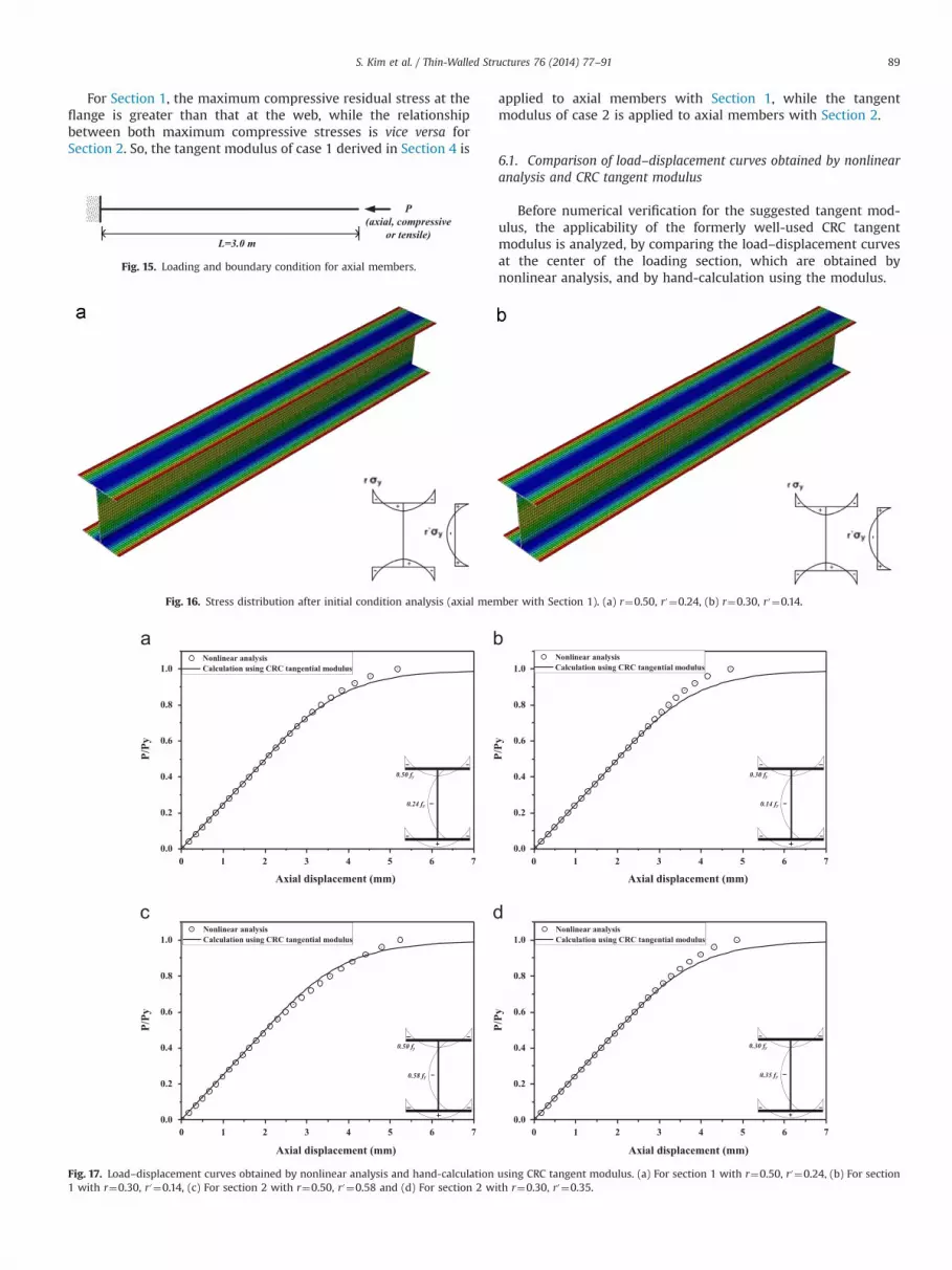
For Section 1, the maximum compressive residual stress at theflange is greater than that at the web, while the relationshipbetween both maximum compressive stresses is vice versa forSection 2. So, the tangent modulus of case 1 derived in Section 4 is

applied to axial members with Section 1, while the tangentmodulus of case 2 is applied to axial members with Section 2.

6.1. Comparison of load–displacement curves obtained by nonlinearanalysis and CRC tangent modulus

Before numerical verification for the suggested tangent mod-ulus, the applicability of the formerly well-used CRC tangentmodulus is analyzed, by comparing the load–displacement curvesat the center of the loading section, which are obtained bynonlinear analysis, and by hand-calculation using the modulus.

Fig. 16. Stress distribution after initial condition analysis (axial member with Section 1). (a) r¼0.50, r′¼0.24, (b) r¼0.30, r′¼0.14.

0 1 2 3 4 5 6 70.0

0.2

0.4

0.6

0.8

1.0

P/Py

Axial displacement (mm)0 1 2 3 4 5 6 7

0.0

0.2

0.4

0.6

0.8

1.0

P/Py

Axial displacement (mm)

0 1 2 3 4 5 6 70.0

0.2

0.4

0.6

0.8

1.0

P/Py

Axial displacement (mm)

0 1 2 3 4 5 6 70.0

0.2

0.4

0.6

0.8

1.0

P/Py

Axial displacement (mm)

Fig. 17. Load–displacement curves obtained by nonlinear analysis and hand-calculation using CRC tangent modulus. (a) For section 1 with r¼0.50, r′¼0.24, (b) For section1 with r¼0.30, r′¼0.14, (c) For section 2 with r¼0.50, r′¼0.58 and (d) For section 2 with r¼0.30, r′¼0.35.

L=3.0 m

P(axial, compressive

or tensile)

Fig. 15. Loading and boundary condition for axial members.

S. Kim et al. / Thin-Walled Structures 76 (2014) 77–91 89

0 1 2 3 4 5 60.0

0.2

0.4

0.6

0.8

1.0P/

Py

Axial displacement (mm)0 1 2 3 4 5 6

0.0

0.2

0.4

0.6

0.8

1.0

P/Py

Axial displacement (mm)

0 1 2 3 4 5 60.0

0.2

0.4

0.6

0.8

1.0

P/Py

Axial displacement (mm)0 1 2 3 4 5 6

0.0

0.2

0.4

0.6

0.8

1.0

P/Py

Axial displacement (mm)

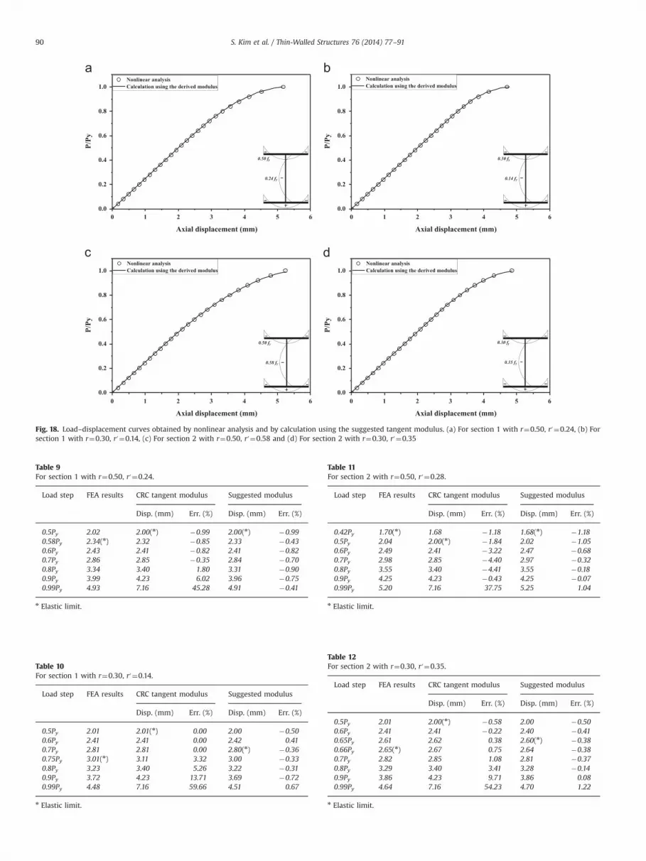
Fig. 18. Load–displacement curves obtained by nonlinear analysis and by calculation using the suggested tangent modulus. (a) For section 1 with r¼0.50, r′¼0.24, (b) Forsection 1 with r¼0.30, r′¼0.14, (c) For section 2 with r¼0.50, r′¼0.58 and (d) For section 2 with r¼0.30, r′¼0.35

Table 9For section 1 with r¼0.50, r′¼0.24.

Load step FEA results CRC tangent modulus Suggested modulus

Disp. (mm) Err. (%) Disp. (mm) Err. (%)

0.5Py 2.02 2.00(n) �0.99 2.00(n) �0.990.58Py 2.34(n) 2.32 �0.85 2.33 �0.430.6Py 2.43 2.41 �0.82 2.41 �0.820.7Py 2.86 2.85 �0.35 2.84 �0.700.8Py 3.34 3.40 1.80 3.31 �0.900.9Py 3.99 4.23 6.02 3.96 �0.750.99Py 4.93 7.16 45.28 4.91 �0.41

n Elastic limit.

Table 10For section 1 with r¼0.30, r′¼0.14.

Load step FEA results CRC tangent modulus Suggested modulus

Disp. (mm) Err. (%) Disp. (mm) Err. (%)

0.5Py 2.01 2.01(n) 0.00 2.00 �0.500.6Py 2.41 2.41 0.00 2.42 0.410.7Py 2.81 2.81 0.00 2.80(n) �0.360.75Py 3.01(n) 3.11 3.32 3.00 �0.330.8Py 3.23 3.40 5.26 3.22 �0.310.9Py 3.72 4.23 13.71 3.69 �0.720.99Py 4.48 7.16 59.66 4.51 0.67

n Elastic limit.

Table 11For section 2 with r¼0.50, r′¼0.28.

Load step FEA results CRC tangent modulus Suggested modulus

Disp. (mm) Err. (%) Disp. (mm) Err. (%)

0.42Py 1.70(n) 1.68 �1.18 1.68(n) �1.180.5Py 2.04 2.00(n) �1.84 2.02 �1.050.6Py 2.49 2.41 �3.22 2.47 �0.680.7Py 2.98 2.85 �4.40 2.97 �0.320.8Py 3.55 3.40 �4.41 3.55 �0.180.9Py 4.25 4.23 �0.43 4.25 �0.070.99Py 5.20 7.16 37.75 5.25 1.04

n Elastic limit.

Table 12For section 2 with r¼0.30, r′¼0.35.

Load step FEA results CRC tangent modulus Suggested modulus

Disp. (mm) Err. (%) Disp. (mm) Err. (%)

0.5Py 2.01 2.00(n) �0.58 2.00 �0.500.6Py 2.41 2.41 �0.22 2.40 �0.410.65Py 2.61 2.62 0.38 2.60(n) �0.380.66Py 2.65(n) 2.67 0.75 2.64 �0.380.7Py 2.82 2.85 1.08 2.81 �0.370.8Py 3.29 3.40 3.41 3.28 �0.140.9Py 3.86 4.23 9.71 3.86 0.080.99Py 4.64 7.16 54.23 4.70 1.22

n Elastic limit.

S. Kim et al. / Thin-Walled Structures 76 (2014) 77–9190

Fig. 17 shows the comparison results of the curves obtained byeach method. As shown in the figure, there is difference in thepaths, as well as in the elastic limit points between the curvesobtained by both methods. The CRC tangent modulus was derivedby assuming the maximum compressive residual stress to be 50.0%of the yield stress of the material. In addition, the equation wasalso derived without consideration of the characteristics of resi-dual stress distributions and sectional shapes. Thus, the modulusmay lead to an inaccurate structural response in inelastic states,because of the limitation of the consideration. In particular, whenthe maximum residual stress is not 50.0% of the yield stress, themodulus leads to significant errors, as shown in the figure.

6.2. Comparison of load–displacement curves obtained by nonlinearanalysis and the suggested tangent modulus

In these paragraphs, the accuracy and applicability of thesuggested tangent modulus that considers parabolic residualstress distribution are represented, based on nonlinear analysisresults.

As shown in Fig. 18, both load–displacement curves extracted atthe centroid of the loading section by nonlinear analysis and bycalculation using the suggested tangent modulus are almost thesame as each other. The elastic limit forces at both comparedcurves are slightly different, because the residual stresses appliedto each finite element were calculated by the interpolation ofparabolic distributions. Despite this, the paths of both comparedcurves that show the inelastic structural responses induced byparabolic residual stress distribution are almost the same.

As shown in the tables, analysis results using the derivedtangent modulus show excellent accuracy for the inelasticbehavior of axial members that have parabolic residual stressdistribution. So, it can be concluded that the suggested tangentmodulus derived based on the force-equilibrium exactly reflectsthe inelastic state of an axial member that has linear and parabolicresidual stress distributions, which have been well considered asgeneral residual stress patterns (Tables 9–12).

7. Conclusion

In this study, the tangent moduli of axially loaded steel membersof hot rolled I-shaped section were derived for generally-used linearand parabolic residual stress distributions based on the principle offorce equilibrium. Using the equations for the derived tangentmodulus, maximum residual stress values can be taken into account

as well as the residual stress pattern and the dimensional char-acteristics of the analyzed section. For the verification of the derivedequations, a series of material nonlinear analyses were performedusing I-shaped axial members modeled by shell elements. Throughthe comparison of results obtained by material nonlinear analyseswith those by the suggested tangent moduli equations, the accuracyand applicability of the presented equations for tangent moduliwere sufficiently verified. It was shown through the extensivecomparative study that the elasto-plastic structural response ofaxially loaded steel members subjected to linear or parabolicresidual stress distribution can be accurately predicted in extremelysimple manner using the suggested tangent modulus.

Acknowledgments

This research was supported by a grant (10CTIPB01-ModularBridge Research & Business Development Consortium) from SmartCivil Infrastructure Research Program funded by Ministry of Land,Infrastructure and Transport of Korea Government and KoreaAgency for Infrastructure Technology Advancement.

References

[1] Galambos TV. Guide to stability design criteria for metal structures. 4th ed.. .New York, USA: John Wiley & Sons; 1988.

[2] Chen WF, Lui EM. Stability design of steel frames. Boca Raton, FL, USA: CRCPress; 1992.

[3] Liew JYR, White DW, Chen WF. Second-order refined plastic hinge analysis forframe design: part I and II. J Struct Eng 1993;119(11):3196–237.

[4] Chen WF. Liew JYR. Implications of using refined plastic hinge analysis for loadand resistance factor design. Thin-Walled Struct 1994;20:17–47.

[5] Kim SE, Chen WF. Practical advanced analysis for unbraced steel frame design.J Struct Eng 1996;122(11):1259–65.

[6] Kim SE, Kim MK, Chen WF. Improved refined plastic hinge analysis accountingfor strain reversal. Eng Struct 2002;22:15–25.

[7] Kim SE, Lee J, Park JS. 3-D second-order plastic-hinge analysis accounting forlocal buckling. Eng Struct 2003;25:81–90.

[8] Kim S. Ultimate analysis for steel cable-stayed bridges [Ph.D. Dissertation].Korea University, Seoul, Korea; 2009.

[9] Galambos TV, Ketter RL. Columns under combined bending and thrust. J EngMech Div 1959;85:1–30.

[10] European Convention for Constructional Steelwork (ECCS). Ultimate limit statecalculation of sway frames with rigid joints. Technical Committee 8-StructuralStability Technical Working Group 8.2-System, Publication no. 33; 1984.

[11] Szalai J, Papp F. A new residual stress distribution for hot-rolled I-shapedsections. J Constr Steel Res 2005;61:845–61.

[12] Young BW. Residual stresses in hot-rolled members. IN: Proceedings of IABSEinternational colloquium on column strength, Zurich, Swiss; 1972. p. 25–38.

[13] ABAQUS. Abaqus Analysis User's Manual version 6.10. Dassault SystemesSimulia Corp.; 2010.

S. Kim et al. / Thin-Walled Structures 76 (2014) 77–91 91