A Family of Tangent Algebraic Splines

A Family of TangentAlgebraic Splines

MARCO PALUSZNY

Universidad Central de Venezuela

and

RICHARD R. PATTERSON

Continuous Cubic

Indiana University and Purdue University at Indianapolis

We present an algorithm for creating tangent continuous splines from segments of algebraiccubic curves. The curves used are cubic ovals, and thus are guaranteed convex. Each segment isgiven by an equation which has five coefficients, thus four degrees of freedom available for shapecontrol. We describe shape handles that work via the coet%cients ta control the curve. Eachsegment can be chosen to interpolate one more point and slope and has two additional fullnessparameters to control the shape. This family of curves naturally contains conic splines as asubfamily.

Categories and Subject Descriptors: 1.3.5 [Computer Graphics]: Computational Geometry andObject Modeling—curue, surface, solid and object representations; J.6 [Computer Applica-tions]: Computer-Aided Engineering-computer-aided design

General Terms: Algorithms, Design

Additional Key Words and Phrases: Cubic ovals, cubic splines, implicit curves, interpolation,piecewise algebraic curves

1. INTRODUCTION

In this paper we study splines created from segments of algebraic curves.These are not the usual parametric splines in which each component function

X, Y depends on a parameter t: ( X, Y) = (~(t), g(t)). In an algebraic splineeach segment is given implicitly as a segment of the graph of an implicitequation f( x, y) = O. The subject was initiated by T. W. Sederberg in [21]and [22].

The main advantage of parametric curves is that they are easy to graphand to control using the methods of B-Splines and B&zier curves [7]. The

Authors’ addresses: M. Paluszny, Escuela de Fisica y Matematicas, Facultad de Ciencias,Universidad Central de Venezuela, Apartado 47809, Los Chaguaramos, Caracas 1041-A,Venezuela; R, R. Patterson, Department of Mathematical Sciences, Indiana University-PurdueUniversity at Indianapolis, 402 N. Blackford St., Indianapolis, IN 46202-3216.Permission to copy without fee all or part of this material is granted provided that the copies arenot made or distributed for direct commercial advantage, the ACM copyright notice and the titleof the publication and its date appear, and notice is given that copying is by permission of theAssociation for Computing Machinery. To copy otherwise, or to republish, requires a fee and/orspecific permission.o 1993 ACM 0730 0301/93/0700-0209 $01.50

ACM Transactions on Graphics, Vol. 12, No. 3, July 1993, Pages 209 232.

210 . M. Paluszny and R. R. Patterson

main advantage of implicit curves is the ease of checking whether a given

point lies on, to the right of, or to the left of the curve. Implicit curves of agiven degree greater than two also have more degrees of freedom for shapecontrol.

There are two areas in which much more work is needed in order to makeimplicit curves as useful as parametric curves are: graphing methods andshape control. Graphing methods so far are relatively slow, but are becomingmore sophisticated to provide greater accuracy. Methods studied so farinclude walking along the curve pixel by pixel [4], stepping along the tangentvector and making corrections, taking into account singular points [2],parametrizing the curve by elliptic functions (elliptic curves only) [16], find-ing the intersections of the curve with a triangulation of space [6], andfinding local rational approximations [3]. The curves used in this paper are sopredictable they can be graphed by the most naive method.

Some contributions to the study of shape control of implicit curves aremade by Sederberg [22] in the original paper on this subject. Li, Hoschek, andHartmann study a case in [12] which has one degree of freedom. Sederberg[20] studies the problem of finding intersections of implicit curves, andGarrity and Warren [8, 25] compare several definitions of geometric continu-ity for them. More attention has been given to implicit surfaces [1, 5, 9– 14,19, 21, 23, 24].

This paper is a contribution to the study of shape control of implicit cubics.

The general cubic has ten coefficients, but after endpoint positions andtangents are imposed has six coefficients and five degrees of freedom left. Acomplete geometric analysis of these five degrees of freedom is the ultimategoal, but in this paper we restrict to a subfamily with four degrees offreedom. The curves in this subfamily are arcs of cubic ovals. The shapehandles discussed in this paper are (primarily) interpolation conditions. In a

subsequent paper we will discuss curvature conditions.The individual segments of our splines inherit from cubic ovals the proper-

ties of convexity and nonsingularity. Thus any inflection points or double

points in a spline must be explicitly put in by the user. In addition thesecurves and the splines created from them have the properties

—local control,

—variation diminishing,

—convex hull,

—afflne invariance, and

—quadratic precision.

These curves are a direct generalization of conic splines, which form anatural subfamily. Unlike many spline constructions, there are no knotconsiderations and no global systems of equations to solve.

We begin in Section 2 by reviewing the notation we use for barycentriccoordinates. In Section 3 we review the classification of algebraic cubic

curves. Sederberg’s construction is reviewed in Section 4. In Section 5 wedefine the family of curves we use and prove that they are segments of cubic

ACM Transactionson Graphics,Vol. 12, No. 3, July 1993.

A Family of Tangent Continuous Cubic Algebraic Splines . 211

ovals. The shape handles used for individual segments are described inSections 6 and 7. In Section 8 we describe the spline construction.

2. BARYCENTRIC COORDINATES

Barycentric coordinates in the afflne plane are defined with respect to atriangle. If the vertices PO, ~1, and P2 have Euclidean coordinates PO(X., Y.),PI( x,, Y1 ), and P2( X2, Y2), the Euclidean coordinates (x, y) of any point Pcan be expressed

(X, Y)= S(XI), YO) +t(x,, Yl) +U(X2, Y2)

with s + t + u = 1. Thus P has barycentric coordinates P(s, t, u). Thebarycentric coordinates of the vertices themselves are PO(l, O,O), PI(O, 1, O),and P2(0, O, 1).

Passing between barycentric and Euclidean coordinates is done using amatrix

[)

~o Yo 1

(X, y,l)=(s, t,u) xl Y1 1

X2 Y2 1

and its inverse. Using these substitutions we can write an equation in eitherEuclidean or barycentric coordinates.

Passing from barycentric coordinates to general homogeneous coordinatesbased on the triangle and with its barycenter P( 1/3, 1/3, 1/3) as unit pointis done by sending (s, t, u) to its equivalence class [s, t,u], where (s, t, u) isequivalent to (ks, kt, ku) for k # O. Passing from homogeneous to barycentriccoordinates is possible for those points not on the line at infinitys + t + u = Oby choosing the representative of the class [s, t,u] which satisfies s + t + u

= 1. See [ 17] for more about general homogeneous coordinates.

3. CLASSIFICATION OF CUBICS

In this section we review the classification of real algebraic cubic curves.When its equation can be factored, a cubic is reducible and is either a lineand a conic or three lines. Otherwise the curve is irreducible, in which case itis either singular or nonsingular. A singular cubic has exactly one doublepoint which is either a crunode, an acnode, or a cusp [15]. A nonsingularcubic has either one circuit or two as a curve in the real projective plane. Forthe curves with two circuits, one is the oval, which separates the projectiveplane into a component which is topologically a disk and one which is aMobius band, and the other is the odd circuit, which does not separate theprojective plane; see Figure 1. A cubic with one circuit has only the oddcircuit.

In order to determine from the coefficients of the cubic which type ispresent, we can use a discriminant A defined in [18, pp. 191-192].

THEOREM 3.1. A homogeneous cubic F is irreducible and nonsingular ifand only if A(F) # O. Moreover F has one or two circuits as A(F) > 0 or

A(F) <0, respectively.

ACM Transactions on Graphics, Vol. 12, No. 3, July 1993.

.—


Fig. 1. A two-circuit cubic.

The polynomial A has degree 12 in the 10 coefficients of the general cubicand has over 10,000 terms. However in the case of the cubic we shall beusing,

F(s, t, 24) = as2u + bsu2 – cst2 – dt2u + estu – ft3,

four of the coefficients are zero and the formula for A reduces to

A = a2b2(27a2b2f4 – abe3f3 – 36a2bdef3 – 36ab2cef3 + @e4f2

+bce4f2 + 8a2d2e2f2 + 46abc&2f2 + 8b2c2e2f2 + 16a3d3f2

–24a2bcd2f2 – 24ab2c2df2 + 16b3c3f2 – cde=f – 8acd2e3f

– 8bc2a%3f – 16a2cd3ef + 64abc2d2ef – 16 b2c3&?f – c2d2e4

–8ac2d3e2 – 8bc3d2e2 – 16a2c2d4 + 32abc3d3 – 16b2c4d2),

up to a positive scalar.

4. REVIEW OF SEDERBERG’S CONSTRUCTION

Sederberg [21, 22] has proposed the following idea which we review here forthe case of cubics. It begins with the B6zier construction of triangular surfacepatches. Given a reference triangle POPIP2, some specific points Xij~ in thetriangle are defined by

Xijk= ;Po + ;Pl + ;P2,

for i,~, k >0 and z + ~ + k = 3 as in Figure 2. If a z-coordinate Pijk isassigned tO each point Xij~, the corresponding points (Xi jh, Pijk ) are thecontrol pointa of a triangular B6zier patch; the graph of

()z=qs, t,u)=~ & Pij~SitJUk.Y

ACM Transactions on Graphics,Vol. 12, No. 3, July 1993.


PO. Xm Xml X102 P2 = X003

Fig. 2. The points X,,~ in the triangle.

The intersection of this surface with the plane z = O is a plane curveF’(s, t, u) = O, defined implicitly in terms of the barycentric coordinates of thetriangle. Now there are exactly as many points X,j~ as there are coefficientsin a polynomial of degree 3. So the Pijk can be reinterpreted both as thecoefficients of an implicit equation and as weights at the points X,,k. In thisway every implicit cubic equation, when rewritten in barycentric coordinateswith respect to some triangle, can be thought of as defining the curve ofintersection of a B6zier surface with the plane.

Using this interpretation of an implicit equation, Sederberg describedseveral geometric properties of the curve in terms of the coefficients. Heshowed that if the weight at a vertex of the triangle is zero then the curvepasses through the vertex. Furthermore if an adjoining weight on one edge isalso zero the curve is tangent at the vertex to that side of the triangle. 1 InFigure 3 the points X,,k are labeled with the corresponding coefficients P,Jk.Only that portion of the curve which lies inside the triangle is graphed.

5. CUBIC OVALS

Suppose we are given two points PO and P2 and lines through them whichintersect at a point PI. We are interested in finding convex cubic arcs whichlie within the triangle POPI P2, join PO to P2 and are tangent at PO and P2to the two given lines. If we use this triangle b define barycentric coordinatesas in Section 2, we know from the results of Sederberg that for a cubic

satisfying the interpolation conditions the coefficients of s 3,s 2t, tu 2, and u 3are zero. The equation of such a curve therefore has the form

F(s, t,u) = CIS2U+ bsu2 – cst2 –dt2ZJ + estu –ft3 = O.

The notation has been simplified to avoid the triple subscripts since a gooddeal of algebra must be done with these coefficients. Figure 4 illustrates howthese coefficients and the barycentric coordinates correspond to points in thetriangle.

1This tangency property may be lost if the vertex happens to be a multiple point; see Figure 9b.



o

-1

0

0 1 1 0

Fig.3. Graph of szu + SU2– Stz – t2u = O.

Fig. 4. Notation for the triangle.

P.

.fj=l U=l

We now begin to impose additional conditions on the coefficients so that thecurves in the family include a convex arc within the triangle from P. to P2,tangent to the sides. The first condition is that a and b must have the samesign. This is because the line t! = O intersects the curve in PO, Pz and thepoint P(s, O, u) whose coordinates satisfi as + bu = O. If a and b haveopposite signs, P lies between P. and Pz. To avoid this we now impose thecondition a, b > 0.

Next we impose the condition ~ = O. This causes the curve to pass throughPI; more is said about this at the end of this section.

We can see by example that we have not yet imposed enough conditions tokeep the curve inside the triangle. Figure 5 shows the curve when a = b = 1,

ACM Transactions on Graphics, Vol. 12, No. 3, July 1SS3.


Fig. 5. A curve that lies outside thetriangle.

c = – 1, d = – 1/2, and e = O. This and similar examples suggest that wemight need c, d > 0. The next two results combine to show that in this casewe have a useful subfamily of curves.

THEOREM 5.1. lf a, b,c, d >0, the cubic

F(s, t,u) =aszu + bsuz –cstz

is an irreducible and nonsingular two-circuitcases z

—dt 2u + estu

cubic except in the following

—lf a = O (respectively b = 0), the curve is singular with a double point at PO(respectively Pz~

—lf c = O (respectively d = O), the curve is reducible with a factor u ( respec-tively s);

—If ad = bc and e = O, the curve is reducible

‘(stu) ‘(as +bu)(su - ;t’)

PROOF. If a = O, all three first partial derivatives of F have the roots = 1, t = u = O, so that PO is a double point. Similarly if h = O, P2 is adouble point. The conditions involving c and d are easy to see. Because f = O,the discriminant A reduces to

A = -a2b2c2d2(e4 + 8(ad + bc)e2 + 16(ad – bc)z).

If a, b, c, d >0, A is negative and the curve therefore has two circuits unlessthe factor involving e is zero; in other words

e2 = –4(ad+bc) ~8Z.

The minus sign is impossible and

–4(ad + bc) +8- >0

if and only if

(ad - be)’ <0.

ACM Transactions on Graphics, Vol. 12, No. 3, July 1993


Thus the factor involving e is zero if and only if ad – bc = O and e = O, inwhich case F is reducible as indicated. o

Now that we know the curve normally has two circuits we can ask whichone passes through the points PO and Pz.

THEOREM 5.2. If a, b,c, d >0, the graph of aszu + bsu2 – cstz – dt2u +estu = O includes an arc of a cubic oval which lies inside the triangle, joins POto Pg, and is tangent to the sides of the triangle. If ad – bc = O and e = O, thecurve reduces to a conic arc.

ROOF. The proof entails looking for silhouette points. According to Salmon[18], Articles 167 and 200, from a point on a one-circuit curve, two lines canbe drawn which are tangent to the curve at other points. These points oftangency are silhouette pointa as seen from the given point. From a point onthe odd circuit of a two-circuit curve, four such lines can be drawn—two topoints on the odd circuit and two to points on the oval. From a point on theoval, none can be drawn.

We use this idea to test whether PO lies on the oval, first in the case e = O.Treat PO(l, O, O) as the origin and search for lines through PO which aretangent to the curve. Into aszu + bsu2 – cstz – dtzu = O, a, b >0, substi-tute u = mt and s = 1.2 We get

t[–drntz + (bm2 – c)t + am].

The factor t corresponds to the intersection at PO. The quadratic factor has adouble root if its discriminant G(m) equals O:

G(m) = b2m4 + (4ad – 2bc)m2 + C2 = O.

Thus the question is reduced to whether G has O or 4 real roots, since wehave already determined that the curve has two circuits. In other words, POlies on the oval if and only if the minimum of G is positive. From

G’(m) = 4b2m3 + 4(2ad – bc)m

we see the critical points occur when m = O and

bc – 2ad~z =

b2 “

The value of G at O is positive if c # O. When bc – 2ad <0, 0 is the onlypoint that needs to be considered. So the dotted area in Figure 6 above theline bc – 2 ad = O in c, d-parameter space contains coefllcient values forwhich PO lies on the oval. In addition, when bc – 2 ad > 0 we have those

2No points are missed by ignoring the line t = Othrough PO and P2. It already crosses the curvetwice. It can not be tangent at another point without violating Bezout’s theorem, according towhich a line meets a cubic in at most three points.

Letting s = 1 means we are thinking about homogeneous coordinates rather than affinecoordinates for a silhouette point which does not lie on the line s = O.No such point could lie onthe line s = Osince s = O already meets the curve once at PI and twice at Pz.



d bc-ad=O bc-2ad=0

c

Fig. 6. The region for which P. lies on the oval

points for which the value of G at ~ m is positive. Substituting for m2 wefind

b2G = 4ad(bc – ad).

Thus since d >0, G is positive if and only if bc – ad >0, which adds theregion that is vertically striped.

Repeating the argument with P2 we find the region in c, d-parameterspace that corresponds to having the point P2 on the oval. The intersection ofthe two regions is the first quadrant.

Because PO and P2 lie on the oval when e = O, this remains tme bycontinuity for all e. •l

Finally, we can explain the reason for choosing f = O; this causes the oddcircuit of the curve to pass through PI. With the oval tangent at PO and Pz,each of the lines s = O and u = O has three known intersections with thecubic. Because of Bezout’s theorem the odd circuit has no other intersectionswith these lines and is thus under control safely out of the way.

6. THE CURVE CONSTRUCTION

In this section we describe the parameters used as shape handles to controlthe curve via the coefficients. The shape handles we examine here areadditional interpolation conditions; curvature conditions will be described ina sequel.

We first select a point BO(SO,to, UO) that lies inside the triangle and is to beinterpolated. Second we specify the tangent line at BO. One way to describe itis in terms of the point Q( SI, O, u ~) where the tangent line at B. meets theline P. P2 (it is possible for Q to lie at infinity). A more convenient parameterfor theoretical purposes is the cross ratio R of either the four points Q, BO,



Q.

Q P. s P2

Fig. 7. Defining the cross ratio R.

QO, and Qz shown in Figure 7, or equivalently the four points Q, S, PO, andPz, where S(s./(sO + UO),O, uO/(sO + UO)) is the projection of BO. We obtain

R =R(Q, S, PO, P,) =

so u~S1 u~

so + U. so + u~10

0 1so u~

.sl U1

01so + u~ so + u~

1 0

soul—_—Uosl

For Q between PO and Pz, R is positive, and for Q outside this interval R isnegative. (Another parameter m, more intuitive for a designer, is presentedin Section 8.) The remaining two degrees of freedom are controlled by a pair( PI, Pz ), each of which can vary from O to 1.

THEOREM 6.1. Given a point BO(SO,to, UO) inside the triangle POPIPZ anda point Q(sl, O, u ~) on the line t = O, there exists a cubic in the familyas2u + bsu2 – cst2 – dt 2U + estu = O, a, b, c, d >0 which passes through BOtangent to the line BOQ if and only if Q is outside the interval [PO, Pz ]; S1 <0or S1 > 1. A solution corresponds to a choice of ( /31,& ) in the unit square,with coefficients determined as follows:

C := (1 – f$)sOu:, d := –R(l – ~z)s~uO, e := (1 –R – 2& + 2R~2)sOtOu0.

The proof of Theorem 6.1 is postponed to the Appendix. For the rest of thissection we study properties of this curve construction. In the next section weexamine the effect of the /3’s on the shape of the curve.

If BO is given, because R must be negative the parameter space is theinfinitely long bar in Figure 8. In general each point in this bar determines adifferent oval arc that satisfies the contact conditions at PO, Pz and passes



132

R=o $1

Fig,8. The parameter domain.

through 11o. However certain points determine the reducible curves whichoccur when ad = bc and e = O. When the curve is reducible, the quadraticfactor describes a conic which satisfies the contact conditions and passesthrough BO. Here is an equivalent way to express the reducibility condition interms of the parameters Pl, &, and R.

PROPOSITION 6.2. The curve is reducible if and only if R = – 1 and /31+ /33—— 1; see Figure 8. The arc of the reducible curve is independent of /31and 13zso long as ~, + f3z = 1.

PROOF. From ad – bc = O and e = O, we deduce

R2P2(I –~2) =&(l ‘~1)

and

(1 - 2P, ) =R(l - 262). (1)

Eliminating R we obtain

(P, -132) (B1 +132-1)=0. (2)

Since R is negative we obtain from (1) that 131> 1/2, ~z < 1/2 or thereverse. In either case from (2), @l + p2 = 1. Then from (1), R = – 1. Con-versely if R = – 1 and ~1 + ~t = 1 we can evaluate and find ad – bc = Oand e = O.



When R=-landfll+&=l

t; t:a= —c and b = —d.

SOuo Souo

Letting

~;.y. —

Souo

we have the specific reduction

as2u + bsu2 – cst2 – dt2u = (CS + du)(ysu – t2).

As y is independent of c and d, any change tn c or d or to & or ~2 goesinto a change of the linear factor, not the quadratic. D

In consequence our curves contain the subfamily of conies. Assuming thatwe graph our curves by tracing from PO or P2, in the reducible case the conicarc is what is drawn.

In fact this construction has quadratic precision. Suppose we have a conicarc from PO to P2 within the triangle, with PI the intersection of the tangentlines and with llo(so, to, UO) any interior point of the arc. If we then use thevalue of R determined by the tangent line at l?. and any ~1, f12 such that/31 + /3z = 1, the construction recovers the original conic arc. Because of the

endpoint and tangency conditions on the conic, the coefficients of s 2, st, tu,and u2 are zero. We can then normalize the equation to the form ysu – t 2 = O.Because BO lies on the curve, y = t~/sO UO.The tangent line to the conic at BOhas equation y UOs – 2tOt + yso u = O. This line meets the line POP2 at thepoint Q(sl, O, Ul), where

so –U.51 = and U1 =

so – u~ so — Uo

We find R = – 1. For any @l, ~2 such that /31 + /32 = 1 the curve is reducibleand we recover the original conic.

7. THE EFFECTS OF THE P’S

In this section we investigate the behavior of the curves F = O when B. andthe slope at BO are fixed and the parameters &

The general formula for F is

F(s, t,u) = –R~2t:Uo S2U + &Sot:SU2

+ R(l – ~2)s; uOt2u

vand f12 are varied.

– (1 – pl)sou:stz

+(1 –R – 2& + 2R@2)sOtOuOstu.

This can be factored

(1 - /31)(1 - f12)F00 + (1 - &)~2F01 + ~1(1 - &)FIO + &&F1l. (3)



The formulas for the individual F,j are

Fw = SoUot[– UoSt + ~SotU + (1 – ~)tosu],

FO1 = UoS[–~tjSU – SoUot2 + (1 + R) SOtOtZZ],

FIO = SoU[t;SU + ~So Uot2 – (1 + R)tOuost],

Fll = tOSU[– RtOUOS + (R – l)sOuOt + sOtOu].

These four extremal curves are all reducible. The three lines composing F1,are the sides of the triangle and the line ~. Q. Figure 9 displays the graphs ofthese curves and eight other extreme curves which correspond to values of flland /32 on the edges of the unit square. The curves all interpolate thebarycenter Bo(l\3, 1/3, 1/3) with R = – 1/3.

Because the coefficient of /31(?2 in (3) is zero, we have the identity

FOO– F(J1– FIO + Fll = O.

By evaluating at ( 1/2, O, 1/2) we see that F is positive below the graph ofF = O and negative above. (The meaning of “below,” of course, is relative tothe current orientation of the triangle.) Similarly the quadratic factors of Fw,FO1, and FIO and all three linear factors of F1, are positive at (1/2, O, 1/2).We can use this to show that every oval that corresponds to a point (a,, a2 )in the shaded region in Figure 10 lies above the oval that corresponds to thecorner point ( @l, /3z).

PROPOSITION 7.1. The graph of ~r,, ,,, = O is above the graph of Ffl,,~, = O(except at B,)) if al > pl, a2 > & or if al > P,, CYz> P2.

PROOF. Consider Ffi, ~, = O and FP, , , ~, = O for positive ● . We can writeFP,+e.ti, as

F6,. P, + @l(Foo – Fol –Flo +Fll) + ●(F1o – Foo) = F6,,lj, + ~(Flo – Foo)

Now

FIO – Foo = sos(tou – uOt)2

is positive at any point P other than B. on the graph of FP,,~, = O inside thetriangle. So Ffi, .,, PJP ) is positive except at BO, where it is zero, It followsthat the graph of F@,~,, ~, = O lies above the graph of FP,,~, = O.

A similar argument works for vertical segments. The rest of the prooffollows by transitivity. ❑

The behavior of the curves on the diagonal ~1 = f12 is simple; as the ~‘sare increased the curve swells into the corners. See Figure 11.

The behavior transverse to this diagonal is much more subtle. To explainthis we consider the problem of interpolating another point U. The region inwhich we can choose U is bounded by the graphs of Fw = O and F1, = O andis divided by the graphs of Fol = O and FIO = O; see Figure 12. If U is chosenabove both of the graphs of FO1 = O and Flo = O there are reducible curvesF~;,, and F1 ~i that pass through U. Every curve which corresponds to a

ACM Transactions on Graphics, Vol. 12, No. 3, .July 1993

222 . M. Paluszny and R. R. Palterson

‘R.....

m;0 \=

‘\‘- ..

X\

\,i

/-’

\

--iii

/,\ (K\

‘(\,\\

w-amble a,FXIO,u

“~

T4(,/

\ .

P2 smg.lar

./

\

4‘\. /

(

\

<

/’., /“’” (/‘d \

‘\\.<



(P1!r32)~

Fig. 10, Parameters of the curves that lie aboveF{91,/j2.

Fig. 11. Curves through BO(l/3, 1/3,1/3), m = 0.3 with 131= I?2= .1, .3, .5,.7, .9, .99.

point on the segment between ( ~~, 1) and (1, fl~ ) determines an oval thatpasses through U. Figure 13 illustrates this for a particular point U. Moregenerally the motion along a line of positive slope in the ( f?l, Pz ) controlsquare, say towards ( ~{, 1), corresponds to the swelling of the oval towardsthe conic arc given by ( ~{, 1). Figures 9h and 9i display such arcs.

The point U could alternatively be chosen in the region corresponding to asegment between ( ~ [, 1) and ( ~j, O) (a reducible curve and a singular curve),(O, ~~ ) and (1, ~~) (a singular curve and a reducible curve), or (O, @$) and( ~:, 0) (two singular curves); see Figure 14. Each of these segments musthave negative slope; otherwise the existence of the intersection point Uwould contradict Proposition 7.1.

8. TANGENT CONTINUOUS SPLINES

To create a tangent continuous spline the user chooses a locally convexcontrol polygon that we label as in Figure 15. The control polygon hasendpoints Pf) and Pz,, (which may be the same point), corner points with oddsubscripts and junction points with even subscripts. For tangent continuitythe junction points must be constrained to lie on the segments between



Fig. 12. The region in which another point U can be chosen; Bo(l/4, 1/2, 1/4), m = 0.3.

Fig. 13. A selection of curves through U, Bo(l/4, 1/2, 1/4), m = 0.3.

corner points. The control polygon defines a sequence of triangles. Let A i bethe triangle with vertices Pzi, Pzi, ~, and Pzi, ~. The user selects an interpo-lation point Bi in each Ai, a tangent line at each Bi, and settings for(A[il, P2[Zl) in each Ai, O < PIIz I, P&il s L

Instead of using the parameter R to describe the tangent line at Bi, analternative that is more intuitive is an afhe version of slope. In A~ theparameter nzo = ( – 1, 1) is defined by

1

(

nzo+l nz~-1~. = ?

)thus (sl, ul) = ~m , ~m .

S1 — U1 o 0

This transformation sets up a one-to-one correspondence between points Qthat lie on the line P. Pz but are outside the interval [P., Pz J and the



(O, q

(1+)

(I,p;)

Fig. 14.

(P:,O)

Segments that correspond to pencils of ovals through various points U.

P1

P4‘3 ‘5

P2

Fig. 15 Control polygon

interval ( – 1, 1), with rno = O corresponding to the point at infinity. Thevalue mO = – 1 corresponds to the line through BO and Pz, mO = O corre-sponds to the line parallel to the line POPz, and rno = 1 corresponds to theline through PO.

The relationship between R and mO is given by

sO(mO – 1)R=

SO+ UORand mO =

uO(mO + 1) so – UOR “

When mO corresponds to R, – mO corresponds to I/R.



Conic splines are created if all the fll[ i ] = Pz[ i ] = 0.5 and each m, defaultsto (so – uO)/(sO + UO), where so, to, and UOare the coordinates relative to Aiof B[. These conic splines are modified by moving the interpolation points B,rather than by the usual way of changing weights at the corners, but this isequivalent. Further modification can then be made in any given segment by

varying ~i, /31[i 1 or P2[ i 1, thus moving to cubic segments.The remaining properties of these splines listed in the Introduction are all

fairly obvious except perhaps for afflne invariance. This holds because all theconstructions are afine.

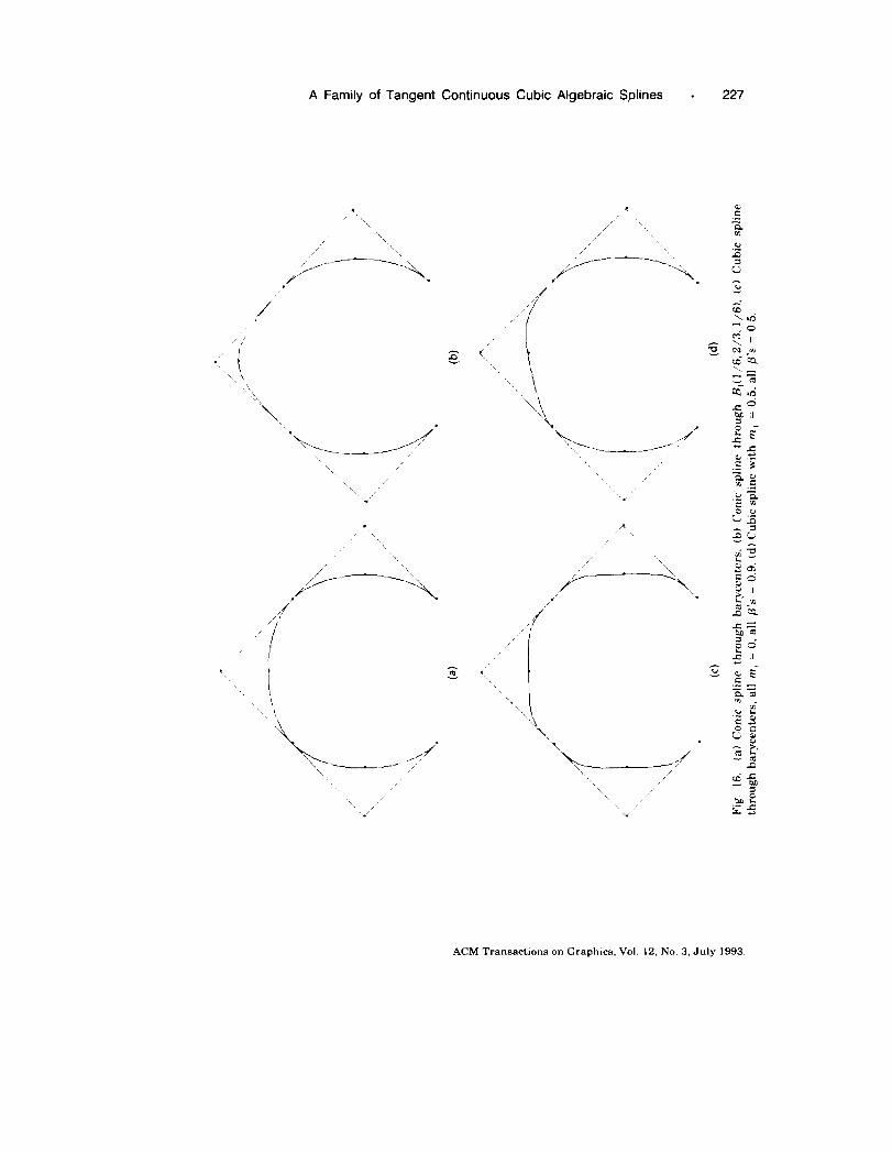
Figure 16a and 16b are conic splines. In 16a, the curves pass through thebarycenters but in 16b, B1 has coordinates (1/6, 2/3, 1/6). In 16c and 16dbarycenters are used again. In 16c all the m, = O and all the B‘s = 0.9. In16d ml = 0.5 and all the P’s = 0.5.

APPENDIX — PROOF OF THEOREM 6.1

The condition that the curve should pass through 130 gives the first require-ment

as~uO + bsOu~ + esOtOuO = csOt~ + dt~u O.

The condition that the tangent line should pass through Q( Sl, O, u ~) gives thesecond requirement

asO(2u Osl + soul) + ?MO(UOSI + 2SOUI) + eto(uosl + soul) = ct~sl + dt~ul.

The two requirements can be written together in matrix form

(aso, Iwo, eto)

or

1

2UOS1 + soul Souo

Uosl +2 SOU1 SouoUosl + soul SOuo

I 2U:S1 –S; U1 — sou~ul \

I– 2S; U1 = (C, d).

— S:ulI(Uso, ~uo,e~o)t:(uos, _ soul) U;SI+ SOUO%

U;sl

Introducing the notation R = so ul\uo S1, we shorten the above formula to

[

2U0 –s.(l + R)

(aso, buO, eto)t;(l!R) Uo(l + R) –2sOR

)

= (c, d).

U. –SOR

We are seeking solutions with both (a, b) and (c, d) in the first quadrant.One condition may be imposed on the five coefficients. We select temporar-

ily the conditionas. + 13uo= 1

in addition to the requirement a, b > 0. With this normalization conditionthe point (aso, buo, eto) can be written aso(l, O, eto) + buo(O, 1, eto). Let wl(e)



*‘ .,

‘....,

\,/‘

.,’.,--.-.<>,

,/’ -N.

;/

“..‘. ‘(~\.\\~.

.

.. . .,

\

./ ‘,.-— — ----.2,

,1.5=‘\

,.{,,,,///

, 1 %“ ‘~

\..

\___ _,/””\

ACM Transactions on Graphics, Vol. 12, N0.3, JuIY 1993.


and wz(e) be the transforms using the matrix above of (1, O, eto) and (O, 1, eto),respectively. Then the point (asO, buo, eto) transforms to (c, d) = asOw ~(e) +buOwz(e). We can express zul(e) and w.Je) in the following way:

~o(l[R)[(uo,-s.) + (1 +eto)(uo, -sol?)]wl(e) = ~

and

1wz(e) = ~ [R(uO, -SO) + (1 +et,)(uo, -.sOR)].

to(l– l?)

Because so and U. are positive, if R is negative, the point

v, =t:(l:R)(uO>-sO)

is in the fourth quadrant,

V2 = ,8(I:R)-”)is in the second quadrant, and

w= ~,(1:R, (uo, -Rso)o

is in the first quadrant of the c, d plane; see Figure 17. As e is allowed tovary, the points wl(e) = VI + (1 + eto)W and wz(e) = Vz + (1 + eto)W slidealong parallel lines lb and 1.. The point asowl(e) + buowz(e) lies on asegment which runs between the parallel lines. Because of the requirementc,d > 0, the domain of variability of (c, d) is the shaded region in Figure 17where the band meets the first quadrant.

If R if positive, the corresponding constructions for the cases O < R <1and R > 1 lead to bands that do not intersect the first quadrant; see Figure18. Hence there is no solution to the interpolation problem if Q lies in[P,, p,l.

We can now obtain expressions in the case R is negative for e, a, and b interms of c and d chosen in the domain of variability. The equation of the linethrough zul(e) and wz(e) is independent of R:

Sotjc + t~uod = (1 + eto)souo.

Hence

e= ‘[ SO,:C +t:u,d - Souo].Sotou”

(4)

Using two = 1 – as., we can solve

asowl(e) + buowz(e) = (c, d)

ACM Transactions on Graphics, Vol. 12, No. 3, July 1993,

A Family of Tangent Continuous Cubic Algebraic Splines

B

. 229

‘2

v, (e)

7° y’Fig, 17. The domain of variability.

for a. Equating either the first or second component we obtain

a= ~,uo(;_,, [Sot;z?c + t:uod + SOUOR

Similarly

b=SOJ -~) [’o’:~’ + ~:%d + s u,]o

(5)

(6)

The line 10 that passes through the points Wz(e) and Vz has the equation

sot; Rc + t;uod + s~u~l? = o.

The requirement a >0 is equivalent to the condition that (c, d) lie below theline 1“. Similarly the line lb has equation

sOt;Rc + tjuOd + SOUOR= O

and the requirement b > 0 is equivalent to the condition that (c, d) lie abovethe line 1*. To summarize, a point (c, d) chosen from the domain of variabilitydetermines the other coeffkients a, b, and e of a curve which satisfies theinterpolation conditions. The four sides of the domain of variability corre-spond to parameter values of the reducible or singular curves which occurwhen one or more of a, b, c, or d is equal to O.

Because the domain of variability is a quadrilateral in the projective plane,we can apply a projective transformation to transform it to a square. This not


—


(a)

(b)

Fig. 18. The bands in case (a) O < R <1 (b) R >1.

only makes it easier to describe the parameter domain, it turns out tosimplify the formulas.

Using the equations for 1. and lb, we can find the homogeneous coordi-nates of the vertices of the domain of variability (see Figure 17): 0[0, O, 1],A[ –UO, O, t~l?l, B[uo, –soR, 01, and CIO, –sOR, t~]. The homogeneous coor-dinates of the unit square are 0[0, 0,11, Ul[l, 0,11, U[l, 1,11, and UJO, 1,11.



Using the methods of [ 17], we find the matrix M of the projective transforma-tion which sends Ul to C, U to 0, Uz to A, and O to B:

[

–U. o t;

M= () so R

)

–t;R .

u~ —SOR o

The inverse of M is (projectively equivalent to)

[

sOt~R2 sOt; R sOt; R

t:u OR t:uo

)

t:uOR .

SOUOR SOUOR SOUOR

A point [ ~1, /?z, 1] in the square transforms to [uO(l – /+), SOR( & –1),t~(/3,– Rflz )]. From this we obtain formulas for c and d in terms of PIand ~2:

uo(l–p~) SOR( /32 – 1)~=

t:( P] – RP2)and d =

t:( B1 – R132) “

From equations (4), (5), and (6) we then obtain

l–R–2pl+2R& –R~z PIp=tO(& – R&) ‘ a = SO(~l – R&)

,andb=UO(~1 – R@z) “

Because these all have the common denominator PI – R /3z, we can cancel it.(Note we no longer have the normalization condition asO + buO = 1 after thiscancellation.) Then if we multiply by sot: UOwe obtain the formulas stated inthe theorem. u

ACKNOWLEDGMENTS

The authors wish to thank Thomas Berry for, among other things, informingthem about the cubic invariants in [18].

REFERENCES

1.

2.

3.

4.

5,

6,

7.

BAJAJ, C. L. Surface fitting using implicit algebraic surface patches. In Topics in SurfaceModeling, H. Hagen, Ed,, SIAM, 1992,BA.JA.J,C. L., HOFFMANN, C. M., HOFCROFT, J. E., AND LYIWH, R. E. Tracing surfaceintersections, (?omput, Aided Geom. Des. 5 (1988), 285–307.BA.JAJ,C. L., ANJJXL, G. Piecewise rational approximation of real algebraic curves. Comput.Sci. Tech. Rep. CAPO 91-19, Purdue Univ., 1991.CHANDLER,R. E. A tracking algorithm for implicitly defined curves. L?LE.EComput. Graph.App[. 8 ( 1988), 83-89.DAHMEN, W. Smooth piecewise quadratic surfaces. In Mathematical Methods in ComputerAided Geometric Design, G. Farin, Ed,, Academic Press, Boston, 1989.DOBKJN, D. P., LEVY,S. V. F., THURSTON,W. P., ANOWILKS,A. R. Contour tracing bypieccwise linear approximations. ACM Trans. Graph. 9, ( 1990), 389-423.FARIN, G. Cur[,es and Surfaces for Computer Aided Geometric Design: A Practical Guide.Academic Press, Boston, 1988.



8. GARRITY,T., ANDWARREN,J. Geometric continuity. Comput. Ai&d Geom. Des. 8 (1991),51-65.

9. HOFFMANN,C. M., AND HOPCROm, J. E. Automatic surface generation in computer aideddesign. Visual Comput. 1 (1985), 95-100.

10. HOFFMANN,C. M., ANDHOPCROn,J. E. The potential method for blending surfaces andcuwes. G%ometric Mo&ling: Algorithms and New Trends, G. Farin, Ed., SIAM, Philadelphia,1987.

11. HOSCHEK,J., ANDHARTMANN, E. Functional splines for interpolation, approximation, blend-ing of curves, surfaces and solids. In Topics in Surfaceitfodehng,H. Hagen, Ed., SIAM, 1992.

12, L1, J., HOSCHEK,J., AND HARTMANN, E. G“ - l-functional splines for interpolation andapproximation of curves, surfaces and solids. Comput. Ai&d Geom. Des. 7 (1990), 209–220.

13. LQDHA,S., ANDWARREN, J. B6zier representation for cubic surface patches. Comput. AidedDes. To appear.

14. LODHA, S., AND WARREN, J. Bi5zier representation for quadric surface patches. Comput.Aided Des. 22 (1990), 574-579.

15. PATTERSON,R. R. Parametric cubics as algebraic curves. Comput. Aided Geom. Des. 5(1988), 139-159.

16. PATTERSON,R. R. Parametrizing and graphing nonsingular cubic curves. Comput. Aided&3. 20 (1988), 615-623.

17. PRNNA, M. A., AND PAITERSON,R. R. Projective Geomet~ and its Applications to ComputerGraphics. Prentice-Hall, Englewood Cliffs, NJ, 1985.

18. SALMON, G. Higher Plane Curves. Hodges, Foster and Figgis, Dublin, 1879.19. SEDERBERG,T. W. Algebraic geometry for surfaces and solid modeling. Geometric Modeling:

Algorithms and New Trends, G. Farin, Ed., SIAM, Philadelphia, 1987.20. SEDERBERG, T. W. Algorithm for algebraic curve intersection. Comput. Ai&d Des. 21

(1989)>547-554.21. SEDERBERG, T. W. Piecewise algebraic surface patches. Comput. Aided Geom. Des. 2

(1985), 53-59.22. SEDERBERG,T. W. Planar piecewise algebraic curves. Comput. Aided Geom. Des. 1 (1984),

241-255.23. WARREN,J. Blending algebraic surfaces. ACM Trans. Graph. 8 (1989), 263-278.24. WARREN, J. Free form blending A technique for creating piecewise implicit surfaces. In

Topics in Surface Mo&ling, H, Hagen, Ed., SIAM, 1992.25. WARREN, J. Several notions of geometric continuity for implicit plane curves. Monografias

de la Academia de Ciencias de Zaragoza, Comunicaciones preeentadas en el Instituto deEstudios Avanzados de la OTAN sobre “Computaci6n de Curvas y Superficies”, Puerto de laCruz (Tenerife, Espaiia, 1989) 2 (1990).

Received January 1!?91;revised May 1992; accepted September 1992

Editor: Anthony DeRose

ACM Transactionson Graphics,Vol. 12, No. 3, July 1993.

Documents

A Family of Tangent Algebraic Splines