An efficient tangent scheme for solving phase-change problems

COMPUTER METHODS IN APPLIED MECHANICS AND ENGINEERING 66 (1988) 65-86 NORTH-HOLLAND

AN EFFICIENT TANGENT SCHEME FOR SOLVING PHASE-CHANGE PROBLEMS

Mario STORTI, Luis A. CRIVELLI and Sergio R. IDELSOHN Mechanics Laboratory, Instituto de Desarrollo Tecnoldgico para la Industria Qu£mica, Universidad

Nacional del Litoral y CONICET, P.O. Box 91, 3000 Santa Fe, Argentina

Received 20 October 1986

Using weak formulations and finite elements to solve heat-conduction problems with phase change finally leads to the solution, at each time step, of a nonlinear system of equations in the nodal temperatures...'~te Newton-Raphson scheme is an effective procedure to cope with this type of problems; however, the choice of a good approximation to the tangent matrix is critical when the latent heat is comparatively large. In this work we derive an exact expression for the tangent matrix and analyze the behavior of its terms for different values of the physical parameters of the system. We demonstrate that this method has good convergence properties. In fact, the rate of convergence is quadratic when the trial approximation is sufficiently close to the solution. Finally, several numerical examples are given.

1. Introduction

Many physical processes of great interest in industrial applications are characterized by substances that undergo a change of phase, such as melting or solidification. This property may be used for energy storage such as in solar energy devices, to obtain new materials as in the metallurgical or glass industries, to predict safety conditions as in the study of the melting of nuclear fuel rods, and many others [1-3].

This problem has been widely studied from a purely mathematical viewpoint [4, 5] to give some insight into the behavior of the solution, such as to demonstrate existence and uniqueness of the solution and the regularity of the temperature distribution under adequate boundary conditions [6]. However, we are far from the possibility of obtaining general analytical solutions, which are restricted to very simplified ~ituations [7, 8]. To overcome this drawback a great deal of effort has been devoted to obtaining accurate numerical solutions.

Basically, the two principal approaches used to solve this problem numerically are the front-tracking algorithms and the fixed domain methods. Front-tracking methods are used mainly in one-dimensional problems for the inherent difficulty in extending them to more dimensions. Furthermore, they cannot cope with multiple interfaces or appearing-disappearing phases. The first available numerical algorithms were of this type and recently an effective and low-cost method using boundary elements has been proposed by O'Neill [9], but they all share the difficulty of requiring a starting solution. Fixed methods, on the other hand, present the advantage of "hiding' the moving front within the weak form of the partial differential equation. Hence there is no need of any tracking and the interface position is determined a

0045-7825/88/$3.50 (f~ 1988 Elsevier Science Publishers B.V. (North-Holland)

66 M. Storti et al., Solution of phase-change problems

posteriori from the temperature results. However they do not have the flexibility of the moving grid algorithms to model sharp gradients near the moving front. We have described here only few important characteristics of both methods, a complete assessment of the different algorithms may be found elsewhere [10, 11].

In this work we have adopted a fixed domain method due to its greater versatility and generality. Within this type of algorithms we can differentiate between enthalpy and regularization methods. In the first one, the enthalpy is the main unknown and the temperature is obtained from the inverse temperature-enthalpy relation [12, 13]. When plotting the resulting temperature distribution, the graph displays a spurious constant temperature region (which is at the melting temperature) known as 'thermal plateaux' [12, 14]. The main drawback of the regularization methods, on the other- hand, is that the solution may depend on the magnitude of the smoothing parameter, as pointed out by Voller et al. [14]. To avoid this problem, a discontinuous integration scheme-~¢sdevised [15, 16], which is used throughout this work.

Phase-change problems are characteh-zed by a jump discontinuity in the enthalpy at the melting/freezing temperature, the magnitude of this jump being equal to the latent heat. Thus, this problem is essentially nonlinear and it is not surprising that the procedures intended for solving the equations arising from the discretized form of the energy equation have difficulties in coping with the steplike behavior of the residual function. Hence, most methods use steepest-descendent or conjugate gradient algorithms. The pioneer work of Meyer [17] uses a method of successive relaxation. Blanchard et al. [18] use conjugate gradients with preconditioning, Voller and Cross [12] use successive overrelaxation SOR. Wintzell [19] develops an explicit expression for the nodal enthalpies as a function of the nodal temperatures. After differentiating he obtains an explicit expression for the Jacobian in the one- dimensional case. He does not extend the procedure to the two-dimensional triangle because it is very cumbersome.

To our knowledge no tangent method has yet been applied to solve this problem. The lack of a Newton (full Newton or modified Newton) method is a direct consequence of the fact that the Jacobian of the system of equations is not known. In this work we present a simple expression for the Jacobian, which can be generalized to any dimension. This Jacobian is physically realized through an additional interface capacity matrix. This matrix notably improves the convergence rate of the system of equations as will be shown in the following sections.

2. Basic equations

We shall consider the heat-conduction problem with phase change [1-4], ciefi~ed by the equation

Oh , - ' - m V O

P Ot q + Q (1)

to be solved in the solid and liquid regions D s and D I. In (1) p is the density, Q is the internal heat generation per unit volume and unit time, t is the time, and q is the heat flux defined by Fourier's law, i.e.

M. Storti et al., Solution of phase-change problems 67

q= - k V T , (2)

where k is the thermal conductivity and T the temperature. For phase-change problems the dnthalpy h presents a sharp discontinuity at the melting temperature and may be defined by the equation, -

h ho + = %(T) dT + L O ( T - Tm)- h scF + h ¢F , (3)

where 0, the Heaviside step function, verifies

Tm)= f for T < T m , O(T- 1 for T > T m .

In (3) cp denotes the specific heat, L the latent heat, and T m the melting temperature. With h cF we denote the enthalpy associated to the transition and with h scr the enthalpy in the absence of a transition.

Equations (1)-(3) together with the appropriate boundary and initial conditions given by (4) below, i.e.,

T= T(x, t) on D r , (4a)

n t k V T = ~(x , t) o n Dq , (4b)

T(x, O)= To(x) in D , (4c)

and the equation of energy at the interface F,

(n'tkVT)~ - ( n ' t k V r ) , . '- p L y ( x , t ) , (5)

completely specify the ~-oblem. In (5) n' is the unit vector normal to the moving boundary surface and v ( x , ~ h e velocity of the moving front along n'.

We may obtainthe weak form of this problem as follows. First, integrate (1) over the solid and liquid domains D s and Din, add the natural boundary condition of (4b) integrated over the bounda~ and the energy equation (5) integrated over the moving front after weighting each equation with appropriate piecewise continuous functions. After this, the Reynold's transport theorem is applied to eliminate the boundary integrals and obtain a set of partial differential equations where the ith equation reads:

f o [ ( O h ) ] f N,(x) - ~ - Q -VtN,(x)q dV + N,~ dS = O, (6) Dq

where the N i are 'kinematically admissible' weighting functions. For simplicity, in (6) we assumed unit density.

Applying finite elements to approximate the temperature distribution and using the same space to span the finite element solution as that used for the weighting functions (Galerkin's

68 M. Storti et ai., Solution of phase-change problems

method) [20], (6) may be recast as a system of ordinary differential equations in the temperature unknown, i.e.,

d d"t H + F=G. (7)

In (7) the typical entries of the above vectors are:

Hi = fo Ni(x)h(T(x)) dr , (8a)

F, = y,, V'N,(x)kVNj(x) rj d r , (8b)

Gi= fo N,:(x)Q dV+ fD Ni(x)q dS, q (8c)

where the Nj, j = 1 , . . . , K stand also for the shape functions and Tj for nodal values of the temperature.

The physical meaning of Hi, Fi, and Gi can be seen from (8), these are respectively the enthalpy contribution to node i, the heat flux to this node, and the applied external flux to the same node.

It is to be noted that the enthalpy becomes a discontinuous function in those elements undergoing a change of phase. It is important to deal appropriately with this discontinuity in order to avoid any losing of latent heat by the algorithm. This drawback is found in some algorithms which use regularization techniques [14, 15]. To obtain the nodal enthalpy accu- rately one must resort to special integration techniques. We developed a discontinuous integration scheme [15, 16] which proved satisfactory both from a theoretical point of view as in the numerical examples performed. In fact, the discontinuous integration is equivalent to an implicit smoothing which never exceeds the size of the element, and goes to zero as the element size decreases. This technique is thoroughly described in [15, 16].

The next step is the time integration of the system (8). A proper formula for the time integration is provided by the well-known a method. Dividing the time interval into subintervals of length At, we can approximate the time derivative of the enthalpy at a point inside the interval as

d lti(t . ) = Hi(t . + At) - lti(t ) d"t At ' (9)

where 0 ~< a ~< 1 and the subscript n denotes values evaluated at the nth time step. For the external flux and the conductivity term we may write,

I f tn+At = G i ( t ' ) d t' -Eta,.

F,(t,,) = (1 - a)F,(tn) + aFi(t.

(10)

+At). (11)


In particular, we have adopted the choice a = i. Using (9) and (11), equation (7) may be recast as a system of nonlinear algebraic equations of the form,

H(t. + At) + AtF(t. + At) = AtG(t. + At) + H(t . ) . (12)

Once the nodal temperatures are known for time tn, (12) represents a set of N equations in the N unknown nodal temperatures at time t n + At. This system may be a written in terms of the two mappings C" R to---> R x and G : R to---> R K as,

C(T(t. + At)= G((T( t . ) ) ,

where T is the K-dimensional nodal temperature vector collecting nodal temperature un- knowns.

The classical iterative solution procedure which was used to solve this problem may be stated as follows: knowing a first approximation Tm(t. + At) to vector T(t. + At) we seek a new solution m+l . T (t. + At) by using the following scheme:

C(Tm(tn + A t ) + K T A T m = G ( T ( t n ) ) , (13a)

T m+'(t n + At)= Tm(tn + At ) + A T m , (13b)

where the tangent matrix K T is obtained as

aC~ (14) [Kd,j = a r j "

Equation (13a) represents a linear system of equations of dimension K x K which may be solved for K T nonsingular.

The mapping C is made up by the contribution of conduction and enthalpy terms. When differentiating C the contribution of the conduction term to the tangent matrix is straightfor- wardly obtained, but we must stress that the enthalpy may have a singularity since h(T) is a discontinuous function at the melting temperature T m. Moreover, splitting the nodal enthalpy vector into two terms, we may write,

I " £ N,(x) h d V , (15)

where H scF corresponds to the nodal enthalpy of a nonlinear problem but -~,lthout a change of phase, and H cF is the change of enthalpy due to the change of phase. The computation of the derivative #H scF/0 T i is straightforward, hence the difficulty lies in obtaining, if it exists, the derivative of the phase change contribution #HCF/o T/.

In fact, taking into account (15) and neglecting nonsymmetric terms, the tangent matrix of (14 ) becomes,

MSCF CF [x.. .] , j = at ,j +_._,j + M,j ,


where K is the conductivity matrix and M scF is the classic capacity matrix [20]. The new term M cr, called interfase-capacity matrix, will be described in the following section.

3. Interface capacity matrix

In the following we shall describe the matrix form of the contribution of the change of phase term to the tangent matrix. This matrix is called the interface matrix since it accounts for the contribution of the terms concentrated on the ii:terface, as will be seen below. Setting the phase-change enthalpy contribution in the form,

HC~ = fo N~(x)LS(T- T~) dV ,

and taking derivatives with respect to T m in the distributional sense [21] we obtain,

0x7 r or(.) - J~,]- N i ( x ) t S ( r - Tin) ~ dV 0Tj

= fD N~(x)L6(T- Tm)Nj(x) dV, (16)

where 8 ( T - Tm) is the Dirac delta function which verifies,

fr {1, Tm ~.[r ,, T2I , r~ 6 ( T - T m) d T = 0 otherwise. 1 ,

The following derivation of the interface mass matrix will be given separately for the linear one-dimensional and quadrilateral elements.

3.1. One-dimensional element

The right-hand side integral in (16) may be written as,

N~(x)L6(T- Tm)N~(x ) dl .

Assuming nondegeneracy of the solution (no real mushy regions), each point of the one-dimensional element has a different temperature, and we have a bijective relation x <--> T. Hence, by changing the independent variable we obtain the relation,

CF _ f <b) M~j j T(a) N (x( T)) LS( T - T )Nj(x( T)) dT

L = Ni(X(Tm)) IVT]m Nj(X(Tm)), (17)


where X(Tm) is the actual x-coordinate of the position of the interface and IVTIm represents the modulus of the temperature gradient evaluated at the interface point.

3.2. Two-dimensional quadrilateral element

For the two-dimensional case the computations are more involved. Let us consider the linear quadrilateral element depicted in Fig. 1. For this element the right-hand side integral in (19) may be recast as

f CF = JD N~(x )8 (T- Tm)Nj(x ) dx 1 dx 2 . M o

Assuming again nondegeneracy of the solution, we seek a transformation of the form (x~, x2) ~ (T, u), where the curves T = constant characterize isothermal lines and u = constant are flux lines, e.g. lines that at each point are perpendicular to an isothermal line. In terms of these new variables, we may write,

f f CF___ Jr J. Ni(T' u ) 8 ( T - Tm)Nj(T, u) det J dT d u , M o (18)

where the Jacobian matrix J is defined by:

J ~

Ox~ OXl ] aT au

OX 2 OX 2 "

OT Ou

(19)

Since the u- and T-curves are perpendicular to each other, we have the additional relation:

i u i 1 Ou = OT " Oxl

(20)

T:constant.

Fig. 1. System of curvilinear coordinates (T, u) for the linear quadrilateral element.


Replacing (20) into (19) gives:

I OT aT] d e t J = d e t -1 aXl Ox2 = 1

0T 0 r / IVTI ~X 2 OX 1 J

hence (18) becomes:

(21)

cF f. L N~(X(Tm) ) du . (22) Mij = N,(x(Tm)) lVrl~ m

In (22) the integral is evaluated over the curved interface. Then it is useful to use the arc-length of the interface as the integration variable. We know that on the interface the arc-length dS is related to du by:

[(aXl~ 2 (aX2~2 ~ 1/2 dS = "~U /m + \ Ou /mj du . (23)

But from the orthogonality of the Jacobian matrices we have,

+ \ Ou OX, I \ aX 2 4;-( )2]

[OTax2 OTaxl] 2 [aTOXl OTOx2] 2 - O~ ~u Ox 2 0 u + Ox 1 Ou +Ox 2"Ou = 1 ,

as can be seen from the product of the Jacobian matrix, given in (19), by its inverse, given in (21). Hence, (23) reduces to:

du = IVTIm dS, (24) i

where the subscript m denotes that the gradient is evaluated on the interface. Finally replace (24) into (22) to obtain,

N,(x) L U,j -- [vr[ m Nj(x) dS. (25)

From (17) and (25) we can see that the influence of the phase change on the capacity matrix is equivalent to that of a capacity of magnitude L/[VTlm per unit length concentrated on the interface. The physical meaning of this result may be seen more clearly through a smoothing technique, i.e. assuming that the change of phase takes place over a finite range of

AT thus obtained temperatures denoted by A T, as depicted in Fig. 2. The equivalent capacity c p is assumed to vary following the temperature-dependent function shown in Fig. 3. The matrix ~H~r ~- i /o~} becomes:


h(Tm) l I ~T : "Mushy " opprox imot ion to t!

. . . . h = Enlo lphy

It,

TIn-AT/2 Tm Tm +~'3:/~) TEMPERATURE

Fig. 2, Regularized enthalpy-temperature function.

M/~r= all/~r

OTi "= fz) C*prNi(x)Nj(x) dV

where

AT Cp - -

= [h(T m + ½AT)- h ( T m - I&T)] ~-~ - %, IT- Tml < IAT,

% [o, I T - Tml > ½AT.

(26)

The first term in the right-hand side of (26) is the matrix M scF. The second is a contribution coming only from the re#on DAr whose temperature is within the range I T - Tmi < ½ A T. This contribution corresponds to the phase-change as shown by the difference,

M~- usc~= fo - - i j (c~ T %)Ni(x)Nj(x ) d V . AT

(27)

From Fig. 4 we can see that in the limit, when T->0 , we have:

AT L dV= dS, A T' I V - I

Cp

c~(T.)

• |

Tm TEMPERATURE

Fig. 3. Equivalent heat capacity-temperature function giving the regular enthalpy of Fig. 2.


Tffi'rm ~

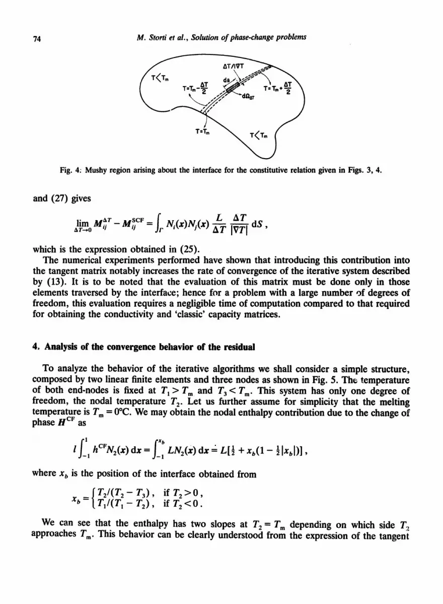
Fig. 4. Mushy region arising about the interface for the constitutive relation given in Figs. 3, 4.

and (27) gives

fr L AT - M scF= N,(x)N](x) AT IV~ lim M~ r _._~j AT--*0

dS,

which is the expression obtained in (25). The numerical experiments performed have shown that introducing this contribution into

the tangent matrix notably increases the rate of convergence of the iterative system described by (13). It is to be noted that the evaluation of this matrix must be done only in those elements traversed by the interface; hence for a problem with a large number of degrees of freedom, this evaluation requires a negligible time of computation compared to that required for obtaining the conductivity and 'classic' capacity matrices.

4. Analysis of the convergence behavior of the residual

To analyze the behavior of the iterative algorithms we shall consider a simple structure, composed by two linear finite elements and three nodes as shown in Fig. 5. The temperature of both end-nodes is fixed at T~ > Tm and T 3 < T m. This system has only one degree of freedom, the nodal temperature T 2. Let us further assume for simplicity that the melting temperature is T m = 0°C. We may obtain the nodal enthalpy contribution due to the change of phase H CF as

fl FI l hCFN2(x)dx = LN2(x)dx " L[½ + Xb(1- ½lXbl)] --1

where x b is the position of the interface obtained from

T2/(T - T 3 ) , i f T 2 > 0 , Xb-- T, / (T~-72) , i f T 2 < 0 .

We can see that the enthalpy has two slopes at T 2 = T m depending on which side Tr~ approaches T m. This behavior can be clearly understood from the expression of the tangent


i _+t

Xb T~

Fig. 5. Simplified 1-dof analysis of the phase-change problem.

matrix given by (17). For the problem under study, (17) gives,

OH cv N2(xb)LN2(Xb)

0 r 2 IVTI~ Making T2 ~ 0 , which implies x b --->0, N 2--~ 1, we have:

au~ ~ , W2--,0 ÷ ,

= 1 T2._> 0 _ "

The remaining contributions to the residual vector may be obtained as follows. The contribution uscF -- 2 to the nodal enthalpy and the contribution F 2 from the conduction heat flux are, respectively,

HSCr = Cpl[~ T 2 + ~(r~ + T3) ] 2

F2 = [T~ + T 3 - 2T2 lk l l .

This gives an equilibrium equation for node 2 at time tn of the form,

_ 1L( + ) ) ] + o, -~tt [llcpT2 + --f (28)

where we have taken a = 1 (backward Eu|er) for the time integration. The constant A accounts for the enthalpy at time tn_ ~ and for the load term aris~iag from fixing th, e temperatures T~ and T 3. We shall write (28) in terms of nondimensional variables Y 2 a n d x b ,

defined by,

T~ = T Xb t*= t r , - r m ' X ~ - T A--/'


which gives a nondimensional residual,

r ( r * ) = + 2Ste-~ ] T* - T * (½ - IxZ I)(1 - ½ Ix~ l) T* + 2 F o T * - A , (29)

where Fo and Ste are the Fourier and Stefan numbers, defined by

k At pcp(T~ - T3) Fo = Ste =

Cpl 2 ' L

From (29) it can be seen that when Ste>> 1, the linear terms predominate over the phase-change term. Also, for Fo>>Ste -1, the solution process depends mainly on the conduction term probably because of the large time step chosen. Figure 6 shows the function r = r ( T ) + A for a given value of Fo and Ste.

The numerical results obtained for this problem illustrate the behavior of the algorithm proposed by (13) for a system of many degrees of freedom. When the phase-change mass matrix is not included in the expression for the tangent matrix, the nodal residual r 2 = C 2 - G 2 rapidly goes to zero on~ ~ "n those nodes not connected to an element traversed by the interface. In the elements connected to such elements, the residual remains comparatively large. In this case the convergence rate is equivalent to that of a secant process, i.e. Ilrm+lll < Cllrmll, in contrast t o t h e tangent ra te Ilrm+lll < Cllrmll 2

This is a clear demonstration that the iteration matrix is no longer the tangent matrix but a secant approximation to it. The behavior of the residual for nodes close to the interface is similiar to that for node 2 of the ~xample described above. In the following we study this behavior in more detail.

It is a well-known fact that, for a monotonically increasing function f ( y ) , it is possible to obtain a root f o r / ( Y ) = f o in the interval f ( a ) < f o < f (b ) through the following iterative scheme [22]:

y~ + l = y~ _ f ( Y i ) _ f0 , s

if and only if

[ f ( y ' + l ) - f ( y ' ) l > ( 1 - - ~ , ) s [ y '+1 - y ' [ , 0 < v <1,

-2.O

TI = 1 g . l ~ ~ T z

Ta = -Q25

Ste =0.25 -1.0 (2+2Fo)=1

-o2 -o, / ', ~ : I

Q1 0.2 Tz

-t.0 Fig. 6. Residual r = r(T) + A as a function of the nodal temperature T 2.

M. Storti et al., Solution of phase-change problems

If(yi+~)-f(yi)l<(1 +/3)slyi+~-y~l, 0 < / 3 < 1 .

Furthermore, the approximation is bounded by

[ f + l _ y'l < m a x ( , / , fl)[y~ - y i - ~ [ ,

for we have

S

and, since f is monotonic,

( - ) s i g n ( y ' - y'-~) - sign f (y ' ) f ( y , - l ) $ '

we obtain for

,y,_ y,-,, > lf(Y')- f(Y'-') l $

if+~_ f[ < i f _ yi-~[_ l.f(Yi)- f(yi-l) [ < */[Yi - Y'-~I $

and for

$

ly'"'- y'l < I :(''') -:<Y'-')[-s ly'- y'-'l < #ly'- y'-'l. If/3 - 1 for any pair of values y', yi+ 1, then the scheme might fall into a numerical trap (see

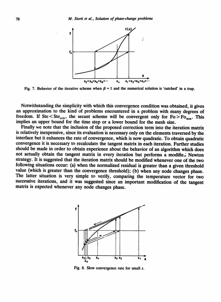
Fig. 7). If the slope near the solution is close to 2s, the rate of convergence could be very low, as shown in Fig. 8. This situation also occurs when the slope is very small compared to s (see Fig. 9), that is, when 3, is close to one. For our problem, not including the interface capacity

CF matrix M ~ implies iterating with a slope s - 2(-~ + Fo). The maximum value of the derivative of the residual in the interval will be,

a r max ~-~ = 2(~ + Fo) + Ste- ' (T, - T3)/min(lT~l, [T~I).

77

2(~ + F o ) > S te - ' (T , - T3)/min(lTll, I T 3 t ) •

Since the term corresponding to the change of phase is monotonically increasing, 3, = 0, this implies that ~imations as given by Fig. 9 could not occur and the condition for convergence for this problem without using the interface capacity matrix gives


J f x2= x4=x6=x8 = . . . . x o

J

X

X t =x3=xS=x7 =...~

Fig. 7. Behavior of the iterative scheme when/3 = 1 and the numerical solution is 'catched' in a trap.

Notwithstanding the simplicity with which this convergence condition was obtained, it gives an approximation to the kind of problems encountered in a problem with many degrees of freedom. If Ste<Stecrit, the secant scheme will be convergent only for Fo > Fomi n. T h i s

implies an upper bound for the time step or a lower bound for the mesh size. Finally we note that the inclusion of the proposed correction term into the iteration matrix

is relatively inexpensive, since its evaluation is necessary only on the elements traversed by the interface but it enhances the rate of convergence, which is now quadratic. To obtain quadratic convergence it is necessary to recalculate the tangent matrix in each iteration. Further studies should be made in order to obtain experience about the behavior of an algorithm which does not actually obtain the tangent matrix in every iteration but performs a modifie2 Newton strategy. It is suggested that the iteration matrix should be modified whenever one of the two following situations occur: (a) when the normalized residual is greater than a given threshold value (which is greater than the convergence threshold); (b) when any node changes phase. The latter situation is very simple to verify, comparing the temperature vector for two successive iterations, and it was suggested since an important modification of the tangent matrix is expected whenever any node changes phase.

X2~ X6 Xo X5 X3 X4

Xl X

Fig. 8. Slow convergence rate for small s.


.t ! !

XsX4X3 X2 Xt

. _~

Xo X

Fig. 9. Slow convergence rate when s is large compared to the true slope.

5. Numerical examples

The effectiveness of the proposed modification has been tested in many different examples. Fig. 10 shows comparative histograms for the number of iterations necessary for convergence of the iterative algorithm of (13), with and without the interface capacity matrix. The problem studied consists of a rod of length 1 - 1 m, unit thermal conductivity and heat capacity, with melting temperature T m = - 1°C, initially at T(x, 0 ) - 0°C. At t - 0 the temperature on one end is lowered to - 2°C and adiabatic conditions are assumed on the other end. We performed different experiments for various latent heat values L ( - Ste -~) and time steps At (= Fo). In Fig. 10 each histogram represents an experiment for a given At and L. For each time step the height of the columns represents the number of iterations necessary to obtain convergence defined by a normalized residual smaller than 10 -6, i.e.,

IIRII < e , : 10 -6 . IIFII

The successive columns of each histogram correspond to successive time steps fi~r the same run. The truncated columns co~espond to time steps where convergence was not achieved in the first 30 iterations. When the residual behaves in a way that we may predict that

m 0 L:S.At=! L:S.AI:05 C=5. At : 0 2 L ,5 . At*O t L=5. At'OO5

mr . . 0 m :E L:tO.f i t , ! L=tO.~,l'0.5 Ls IO .G t ' 02 L ,50 ,A t , t ~ . : 5 0 . ~ - 0 5

t0

0

Fig. 10. Comparative histograms for the rate of convergence of the residual in a unidimensional phase-change model problem with and without interface capacity matrix.


convergence would not be achieved even for a greater number of iterations, see Fig. 11, the symbol oo has been drawn on top of the column.

From Figs. 10 and 11 one can infer that the behavior of the iterative scheme is greatly improved by the addition of the interface capacity matrix. For further details, in Fig. 11 we show the behavior of the logarithm of the normalized residual for two different times for the case L = 10, At = I in Fig. 10. It also observes a quadratic rate of convergence of the residual when using the interface capacity matrix.

We shall further study the behavior of the iterative scheme without an interface capacity matrix for the problem with L = 5 in Fig. 10. It can be seen that for the time steps At of 1, 0.5, 0.2, 0.1, 0.05 s, the time integration algorithm is stopped at the times t of 2.0. 1.5, 0.8, 0.4, and 0.2 s, due to lack of convergence (we consider that the iterative scheme should be stopped when convergence has not been attained in 30 iterations). It can be seen that reducing the time step does not improve the convergence rate, but on the contrary, the process becomes spoiled at smaller times. This behavior is coherent with the conclusions drawn from the 3-node example analyzed previously. We have seen there that when the interface capacity matrix is not included, reducing the time step does not enhance the rate of convergence, but makes it worse.

The second example consist of a square region A B C D (see Fig. 12) of length 1 m and with 3 0 constant physical properties, conductivity k = 1 W/m °C, heat capacity pcp= 1 J /m C, latent

heat L = 10J/m 3, and melting temperature T m =0°C. For t < 0 the temperature is uniform and equal to 0.3°C. For t > 0 the temperature on sides A B and CD is set equal to - 1.0°C. The Stefan number for this problem is defined as

S t e = ° (T_ _cp_ ...-T~)=O.1. L

Two meshes were used to test the convergence of the method. The first one (Fig. 12(a)) is uniform and relatively coarse (121 linear quad elements), while the other, shown in Fig. 12(b) (900 linear quad elements), is refined using Bezier interpolation near the sides A B and CD, where the temperature is imposed and large gradients are expected to occur. Figures 13 and 14 show the isotherms obtained at times t = 0.6 s and t = 1.0 s, respectively. A full line is used to

1

R1o "410- 2 ~ " ........

t0 - 6 0 5

L:IO.O " ' ' " , , A t : t.0

~ . . o . to =0.0

I I I ~. to ITER ts

S t0 I T E R ts

~ - . . . . . . . . . . s . . - ~ ' , .~ , . , ,~ ,

\ L--100

10-" [ \ [ - - ~ ~,--1 o

10-e I t ~ i I f m 0

Fig. 11. Behavior of the residual function in the first and second time steps ;or oiven Stefan and Fourier numbers in the one-dimensional model problem.


Y~

tO

Of ,f

001 " - ' ' - ,~

OOc ~O.Ot

(a)

¢ f.O x

tO

oo DOO 10 x

(b)

Fig. 12. (a) Coarser mesh and (b) refined mesh for a two-dimensional test problem.

plot the results obtained for the mesh depicted in Fig. 12(b) and dashed line for results pertaining to the mesh given in Fig. 12(a). Coincidence between both results is observed. The distance A E in Figs. 13 and 14 has been compared with the penetration depth of the interface in the semi-infinite problem for which an exact solution is obtained. This comparison is adequate for points where the influence of the boundary conditions imposed on sides BC or CD is negligible, i.e. for points far away from the corner A. Coincidence up to 3% has been verified always in such points. Furthermore, one expects a correct prediction of the position of the interface since the algorithm verifies exactly the enthalpy balance and the heat involved corresponds mainly to latent heat effects instead of sensible heat since Ste ,~ 1.

A E

i

I

/U

\ \ \ \ \ x',. \ ' ,

o o - - '

,N " ~ - . 7 " ~ ' ~ ' - - ~ - o z . -

~ ' ~ . . _ " " -0.4

~.~.~ ~'~'~-~'-----o6---- . . . . , " -08

I -1.0 0

Fig. 13. Isotherms after 0.6 s for the square region of Fig. 12. Full line represents results for the refined mesh of Fig. 12(b).


!.0

E B

-08-.-----

ITER

D C

Fig. 14. Isotherms after 1 s for the square region of Fig. 12. Full line represents results for the refined mesh of Fig. 12(b).

Figure 15 is a histogram showing the number of iterations needed to reduce the residue to a value smaller 4 than 10- . In this figure, each column corresponds to a time step. There is a significant reduction of the number of iterations required when including the interface capacity matrix. Figure 16 shows typical convergence processes ~o~' two time steps with and without M cF.

In the third example we study the freezing of soil when water at 5°C is circulating in a buried pipe. Figure 17 shows the geometry of a plane section perpendicular to the axis of the pipe and depicts the mesh of 186 elements used in the discretization. By using the symmetry of reflection about the line A D , the analysis was restricted to the region A B C D E F A . The geometric dimensions are B C = A B = 1 m, FE = 0.1 m, and A F = 0.2 m. The physical proper-

50.

20-

tO-

O O0 i

01'25

Ill ~HH

0250 o~375 0500 t

Fig. 15. Comparative histograms for the rate of convergence of the residual in a two-dimensional phase-change model problem with and 'without interface capacity matrix.


R

fOO

(b)

lO-Z.

re) 11;1"6]

o ~ Ib ~'~ io ~5 ~o ITER

Fig. 16. Typical behavior o f the residual at two different time steps. Curves a and b arc without M °F while curves c and d are with M °v.

ties for frozen soil are k= 1 .9W/mK, pcp = 1.59x 106jim3 .v.,. for unfrozen soil, k= 1.35 W/m K, pcp = 1.64 x 105 J i m 3 K; the melting tempera~re is T , =0°C and the latent heat L = 7.24 x l0 T J im 3. Adiabatic conditions were imposed- on sides AB, CD, DE, and AF. The temperature of the pipe was fixed at the same value as the temperature of the circulating fluid Tf = I*C and convective heat transfer is assumed to occur on the surface AB, i.e.,

qtll = h(T- T a ) 413 ,

where the film coefficient is h = 1.5764 W / m 2 K. This law is obtained using standard correla- tions [23] for convective heat transfer with natural convection between a plane surface swept by a cold fluid. The region is initially at a temperature T(x, 0) = T O = 5°(2. At time t = 0 the temperature of the air is suddenly lowered to T o = - 15"C.

Results are depicted in Figs. 18-20 which show the isotherms after 30 days, 40 days, and 50 days, respectively. It is important to observe the two interfaces appearing at t = 50 days.

A F -~rll . . . . I ! ! ! !!!J

l l l l l l m i l l

I"11111 c[~ ~.~.~

I IIII Illl Illl !111 IIII ,.

O

Fig. 17. Finite element ideafization of the huned pipe problem.


- ° =

Fig. 18. Isotherms after 30 days for the buried pipe problem. Fig. 19. Isotherms after 40 days for the buried pipe problem.

INTERFACE

i

Fig. 20. Isotherms after 50 days for the buried pipe problem.

Clearly, the interface is not a regular function for this problem. Consequently, front-tracking algorithms could not solve this situation. The method presented in this paper easily handles this sort of situations with no more difficulty than in the case of a single interface.

6. Conclusions

We shall devote some lines to the additional computational expense introduced by the evaluation of the interface capacity matrix. It is to be noted that this matrix is calculated only

M. Stoniet al., Solution of phase-change problems 85

for those elements traversed by the interface. For example, in a two-dimensional structure composed by 100 elements and 121 nodes, when the interface traverses 18 elements, the time required to compute the interface matrix is 0.5 s. For the same problem the mean time required for computing the residual is 9.5 s. The additional cost is therefore 5% (without taking into account the time required for the solution of the linear system). These data have been obtained for a problem with constant thermal conductivity and heat capacity, therefore it is not necessary to reevaluate the conductivity and classical capacity matrices. For temperature-dependent thermal conductivity and heat capacity, the incidence of the evaluation of the interface capacity matrix on the global cost will be much less. Furthermore, the reduction in the number of iterations required to attain convergence has been equal to 70% for problems requiring a threshold for the residual of the order of 10 -6 This reduction in the number of iterations increases when the threshold is reduced due to the quadratic rate of convergence of the tangent algorithm.

Finally we note that all the statistical data for the running time have been obtained in runs performed on a VAX 11-780.

Acknowledgment

Mario Storti and Luis Crivelli wish to acknowledge scholarships received frem Consejo Nacional de Investigaciones Cientificas y Tecnicas (CONICET) in support of this research. We also wish to thank J.F. Weisz in revising the manuscript.

References

[1] [2]

[3]

[4] [5]

[6]

[71 [81

[9]

[10]

[11]

[12]

[13]

A. Fasano and M. Primicerio, Free Boundary Problems: Theory and Applications. (Pitman, London, 1983). J.R. Ockendon and W.R. Hodgkins, eds., Moving Boundary Problem in Heat Flow and Diffusion (Oxford University Press, Oxford, 1975). D.G. Wilson, A.D. Solomon and P.T. Boggs, Moving Boundary Problems (Academic Press, New York, 1978). L.I. Rubenstein, The Stefan problem, Trans. Amer. Math. Soc. (1971). C.M. Elliot and J.R. Ockendon, Weak and Variational Methods for Moving Boundary Problems (Pitman, Boston, 1982). L.A. Caffarelli and L.C. Evans, Continuity of the temperature in the two phase Stefan problem, Arch. Rational Mech. Anal. 81 (1983) 199-224. H.S. Carslaw and J.C. Jaeger, Conduction of Heat in Solids (Oxford University Press, Oxford, 1959). H. Budhia and F. Krieth, Heat transfer with melting or freezing in a wedge, lnternat. J. Heat Mass Transfer 16 (1973) 195-211. K. O'Neill, Boundary integral equation solution of moving boundary phase change problems. Internat. J. Numer. Meths. Engrg. 19 (1983) 1825-1850. J. Crank, How to deal with moving boundaries in thermal problems, in: R.W. Lewis, K. Morgan and O.C. Zienkiewicz, eds., Numerical Methods in Heat Transfer (Wiley, New York, 1981) 177-200. L.A. Crivelli and S.R. Idelsohn, Numerical solution of heat conduction problems with phase-change. Rev. Internat. M6tod. Num6r. Ing. 2 (1985) 43-66 (in Spanish). V.R. Voller and M. Cross, Accurate solutions of moving boundary problems using the tmthalpy method, lnternat. J. Heat Mass Transfer 24 (1981) 545-556. D.R. Atthey, A finite difference scheme for melting problems, J. Inst. Math. Appi. 13 (1974) 353-366.


[14]

[15]

[16]

[171 [181

[19]

[201 [21] [22] [23]

V.R. Voller, M. Cross and EG. Walton, Assessment of weak solution numerical techniques for solving Stefan Problems, in: R.W. Lewis and K. Morgan, eds., Numerical Methods in Thermal Problems (Pineridge Press, Swansea, U.K., 1979) 172-181. L.A. Crivelli and S.R. Idelsohn, A temperature-based finite element solution for phase-change problems, Internat. Numer. Meths. Engrg. 23 (1986) 99-119. M.A. Storti, L.A. Crivelli and S.R. Idelsohn, Making curved interfaces straight in phase-change problems, Internat. J. Numer. Meths. Engrg. 24 (1987) 375-392. G.H. Meyer, Multidimensional Stefan problems, SIAM J. Numer. Anal. 10 (1973) 522-583. D. Blanchard and M. Fredmond, The Stefan problem: Computing without the free boundary. Internat. J. Numer. Meths. Engrg. 20 (1984) 757-771. B. Winzell, Finit element Galerkin methods for multiphase Stefan Problems, Appl. Math. Modelling 7 (1983) 329-346. O.C. Zienkiewicz, The Finite Element Method (McGraw-Hill, London, 3rd. ed., 1977). R. Courant and D. HilberL Methods of Mathematical Physics lI (Interscience, New York, 1962). K.E. Atkinson, An Introduction to Numerical Analysis (Wiley, New York, 1978). D.K. Edwards, Transfer Processes. (Hemisphere, Washington, DC, 1979).

Documents

An efficient tangent scheme for solving phase-change problems