1

Implementation of the Tangent Sphere and Cutting Plane

Methods in the Quantitative Determination of Ligand Binding

Site Burial Depths in Proteins Using FORTRAN 77/90 Language

Vicente M. Reyes, Ph.D.*

E-mail: vmrsbi.RIT.biology@gmail.com

*work done at:

Dept. of Pharmacology, School of Medicine,

University of California, San Diego

9500 Gilman Drive, La Jolla, CA 92093-0636

&

Dept. of Biological Sciences, School of Life Sciences

Rochester Institute of Technology

One Lomb Memorial Drive, Rochester, NY 14623

Abbreviations: CP, cutting plane; TS, tangent sphere; CPM, cutting plane method; TSM, tangent

sphere method; CPi, CP or CPM index; TSi, TS or TSM index; BS, binding site; LBS, ligand BS; GC,

global or molecular centroid; LC, local centroid; PDB, Protein Data Bank

Keywords: protein-ligand interactions; ligand burial; ligand binding site burial; protein centroid; cutting plane

method; tangent sphere method; protein flexibility; protein dynamics

2

1. ABSTRACT:

The degree of ligand burial depth gives an indication of a receptor protein’s flexibility, as the extent of

receptor conformational change required to bind a ligand is thought to vary directly with depth of

burial in the bound state. In a companion paper (Reyes, V.M. 2015a), we report on the Tangent Sphere

(TS) and Cutting Plane (CP) methods - two complementary methods to quantify, in a size-independent

manner, the degree of ligand binding site (LBS) burial in a protein receptor - and their applications. In

this report, we present results that demonstrate the effectiveness of the several FORTRAN 77 and 90

source codes used in the implementation of the two related procedures, as well as the precise

implementation of the procedures themselves. Particularly, we show here that application of the TS and

CP methods on a theoretical model protein in the form of a spherical grid of points accurately portrays

the expected behavior of the TS and CP indices, the predictive parameters obtained from the two

methods, respectively. We additionally show that results of the implementation of the TS and CP

methods on six real protein receptors from the dataset of Laskowski et al. (1996) are in general

agreement with their findings regarding cavity sizes in these proteins. The six FORTRAN program

source codes we present in this report are: (1.) find_molec_centr.f, (2.) tangent_sphere.f, (3.)

find_CP_coeffs.f, (4.) CPM_Neg_Side.f, (5.) CPM_Pos_Side.f and (6.) CPM_Zero_Side.f. The first

program calculates the x-, y- and z-coordinates of the molecular geometric centroid of the protein,

a.k.a., global centroid (GC), which will be the center of the TS. Its radius is the distance between the

GC and the local centroid (LC), which is the centroid of the bound ligand or portion of the LBS. The

second program finds the number of protein atoms inside, outside and on the TS itself. The third

program determines the four coefficients A, B, C and D of the equation of the CP, Ax + By + Cz + D =

0. The CP is the plane tangent to the TS at GC (and thus normal to the line segment connecting GC

and LC). The fourth, fifth and sixth programs determine the number of protein atoms lying on the

negative side, positive side, and on the CP itself. The process is illustrated in Figures 1A and 1B (ibid.,

2015a.).

2. INTRODUCTION:

Most proteins carry out their biological functions in the cell either by binding to small organic molecules called

ligands, or by binding to other proteins, in processes generally termed protein-ligand interactions (PLI) and

protein-protein interactions (PPI), respectively. The two procedures discussed in this paper, namely the Tangent

Sphere Method (TSM) and the Cutting Plane Method (CPM; Reyes, V.M., 2015a; Cheguri, S. & Reyes, V.M.,

2011), were inspired by the initial works by Ben-Shimon, A., et al., (2005); they both deal with PLI (Reyes,

V.M., 2015a, b & c; Reyes, V.M. & Sheth, V.N., 2011), but may be applied to PPI as well (Reyes, V.M.,

2015d). TSM and CPM are complementary, but not redundant, methods of quantifying the degree of burial of a

ligand or LBS in the receptor protein. The initial information needed are the protein centroid coordinates, which

we call the global centroid (GC), and the atomic coordinates of the bound ligand or those of the amino acids

comprising the ligand binding site (LBS), from which the local centroid (LC) may be calculated. The equations

of the CP and the TS are then derived from these coordinates. The quantification is independent of the size of

the protein, therefore the degree of ligand burial in receptor proteins of differing sizes may be directly

compared. The degree of ligand or LBS burial is related to the TS index (TSi) and CP index (CPi) determined

by the TSM and CPM, respectively. The TSi is the percentage of protein atoms inside the TS, while the CPi is

the percentage of protein atoms on the external side of the CP (the side opposite the global centroid).

Knowledge of the degree of burial of a ligand in its receptor protein is important, as it gives one an idea about

the extent of protein conformational change that the protein undergoes upon binding of the ligand. The deeper

the ligand or its BS, the greater the protein conformational change required to bind it, and conversely, the

shallower the ligand or its BS, the lesser the proteinconformational change required to bind it.

The TSM and CPM have also been used as an auxiliary confirmatory test in the 3D tetrahedral search motif

method for predicting specific ligand binding sites in proteins (Reyes, V.M., 2015b & 2015c), as well as the 3D

3

interface search motif tetrahedral pair method for the prediction of protein-protein interaction partners (Reyes,

V.M., 2015d), using the double-centroid reduced representation of proteins (Reyes, V.M. & Sheth, V.N., 2011).

3. DATASETS AND METHODS:

The main dataset upon which the programs presented in this paper can be applied is the Protein Data Bank

(PDB). The PDB is the main international repository for protein 3D structures solved experimentally either by

x-ray crystallography or protein NMR (Berman et al., 2000). To demonstrate the usefulness and efficacy of the

procedures described here, the programs were originally applied to the dataset in Laskowski (1996), composed

of 67 globular (roughly spherical) monomeric enzymes with bound ligand(s). The procedure was also applied

to a “theoretical” protein made by constructing a 3D grid of points in the shape of a sphere of radius 50 units

and with center at the origin, with the points themselves representing protein atoms (Reyes, V.M., 2015a). We

recommend that the present paper be read in conjunction with aforementioned paper in order for the reader to

see precisely how the programs presented here are applied.

The minimum requirements in running the Fortran program source codes reported here is a UNIX computing

environment and a Fortran 77/90 compiler software as all Fortran program source codes must be compiled

before they are run. Source program codes presented in this work were written in either Fortran 77 (Holoien,

M.O. & Behforooz, A., 1991; Mayo, W. & Cwiakala, M., 1994; and Nyhoff, L. & Leestma, S., 1996) or Fortran

90 ( Nyhoff, L. & Leestma, S., 1996 & 1999; Metcalf, M. & Reid, J.K., 1999; and Chapman, S.J., 1997). In

order to apply the procedure in high-throughput batch mode, UNIX C-shell (Powers, S. et al., 2002; Anderson,

G. & Anderson, P., 1986; and Birns, P. et al., 1985) as well as Perl (Tisdall, J., 2001; and Berman, J.J., 2007)

scripts were written. In some complex cases, the scripts were constructed using text manipulation by sed & awk

(Dougherty, D. & Robbins, A., 1997; and Aho et al., 1988).

4. RESULTS AND DISCUSSION:

Tabulated below are the Fortran program source codes presented in this paper. The page numbers refer to the

pages in the present paper where the program starts. We refer the reader to our previous paper, Reyes, V.M.,

2015a, for the implementation and application of these programs. Specifically, please refer to Figures 1A and

1B of said paper.

Table of Programs

--------------------------------------------------------------------------------------------------------------

Program 1: find_molec_centr.f page 7

Program 2: tangent_sphere.f page 8

Program 3: find_CP_coeffs.f page 12

Program 4: CPM_Neg_Side.f page 13

Program 5: CPM_Pos_Side.f page 14 Program 6: CPM_Zero_Side.f page 16

------------------------------------------------------------

4

Most protein PDB files have water molecule coordinates, and these are initially removed by appropriate UNIX

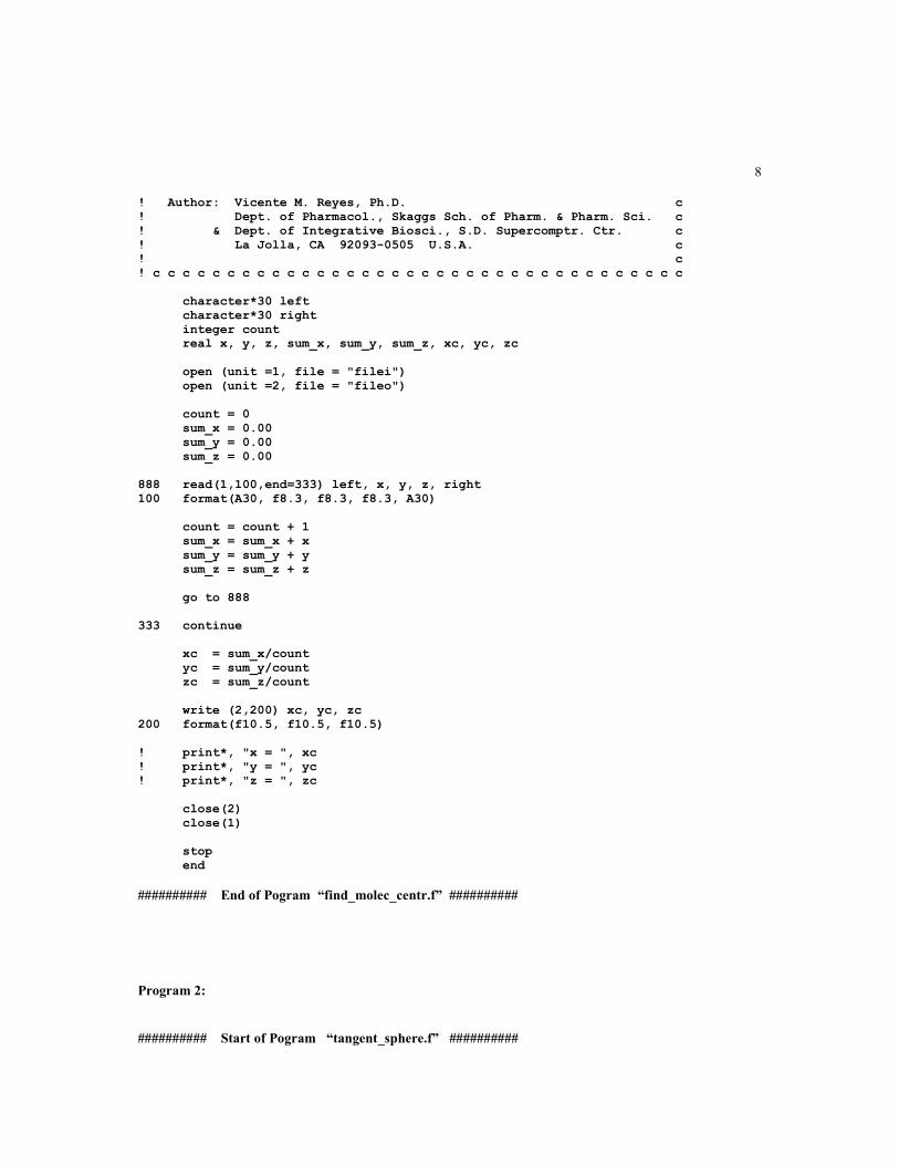
commands. Program 1, find_molec_centr.f, finds the molecular (geometric) centroid of the protein by

averaging the x-, y- and z-coordinates of all atoms in the PDB file of the protein. The result is a single point, (xc,

yc, zc), representing the geometric centroid of the protein molecule. We term it ‘geometric’ centroid because no

weighting was done to account for the different atomic weights of the different protein atoms. The geometric

centroid is the global centroid (GC). The same program may be used to calculate the local centroid (LC), which

is the centroid of the ligand or LBS; it is assumed that some or all of the coordinates of the ligand or LBS are

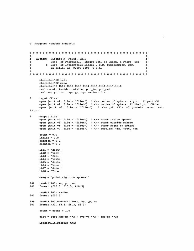
known, which can then be inputted into Program 1. Program 2, tangent_sphere.f, effectively constructs the TS:

it takes in the GC coordinate as center and the distance between the GC and LC coordinates as radius of the TS.

It then outputs the number of protein atoms inside, outside and on the TS. Unsurprisingly, it is quite rare that

atoms are found right on the TS itself. Program 3, find_CP_coeffs.f, calculates the coefficients A, B, C and D

of the equation of the CP, Ax + By + Cz +D = 0, from the GC and LC coordinates and based on the definition

of the CP (see Reyes, V.M., 2015a). Program 4, CPM_Neg_Side.f, determines the number of protein atoms on

the negative side (Ax + By + Cz +D < 0 ) of the CP, while Program 5, CPM_Pos_Side.f, finds the number of

protein atoms on the positive side Ax + By + Cz +D > 0). Finally, program 6, CPM_Zero_Side.f, calculates the

number of protein atoms lying on the CP itself. Again, unsurprisingly, it is rare that protein atoms are found to

lie on the CP itself, so this number is almost always zero. Figures 2A, 2B and 2C (ibid.) show results from the

case of the theoretical spherical protein, while the rest of the Figures (ibid.) show results from the dataset in

Laskowski et al. (1996).

4.1 Implementation of the Programs on a Theoretical Model Protein.

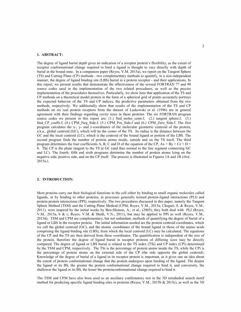
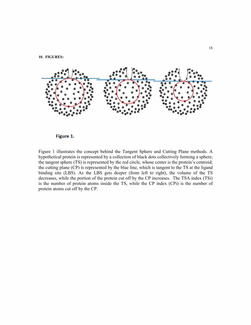
The concept behind the TS and CP methods are illustrated in Figure 1 using the spherical model protein (a.k.a.

theoretical protein). The center of the TS in this case coincides with that of the model protein (grid of points).

The ligand or ligand BS is assumed to be at the bottom of the pit representing the ligand binding pocket and

where it touches the TS. The CP is shown as the blue line tangent to the TS at the same point. As one goes from

the left protein to the right, the LBS depth increases; at the same time, the TS becomes smaller and smaller, and

the CP comes nearer and nearer the center of the protein. The TS index (TSi) is defined as the percentage of

protein atoms lying inside the TS. The CP index (CPi) is defined as the percentage of protein atoms lying on the

external side (the side of the plane opposite the one containing the global centroid (GC). Note that as the LBS

goes from shallow to medium to deep (spherical model protein from left to right), the TSi decreases and the CPi

increases. But that is only half of the story. When the LBS is deep enough that the GC actually lies on the CP,

the behavior of the TSi and the CPi actually reverses as the LBS continues to get deeper.

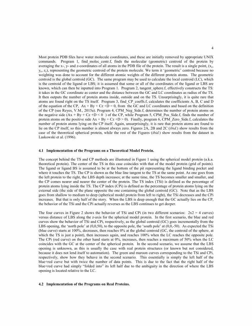
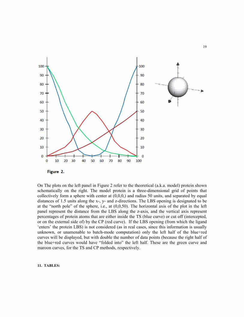
The four curves in Figure 2 shows the behavior of TSi and CPi (in two different scenarios: 2x2 = 4 curves)

versus distance of LBS along the z-axis for the spherical model protein. In the first scenario, the blue and red

curves show the behavior of TSi and CPi, respectively, as the global centroid (GC) goes incrementally from the

LBS opening, the ‘north pole’ at (0,0,50), to the opposite pole, the ‘south pole’ at (0,0,-50). As expected the TSi

(blue curve) starts at 100%, decreases, then reaches 0% at the global centroid (GC, the centroid of the sphere, at

which the TS is just a point), then increases again, and reaches 100% when the LC reaches the opposite pole.

The CPi (red curve) on the other hand starts at 0%, increases, then reaches a maximum of 50% when the LC

coincides with the GC at the center of the spherical protein. In the second scenario, we assume that the LBS

opening is unknown, as this is usually the case with real protein structures (or known but not considered,

because it does not lend itself to automation). The green and maroon curves corresponding to the TSi and CPi,

respectively, show how they behave in the second scenario. This essentially is simply the left half of the

blue+red curve but with twice the number of data points. This is due to the fact that the right half of the

blue+red curve had simply “folded into” its left half due to the ambiguity in the direction of where the LBS

opening is located relative to the LC.

4.2 Implementation of the Programs on Real Proteins.

5

We then tried to implement our procedure to real proteins, which, of course, are not perfectly spherical as the

model protein we described above. Table 1 shows the identities of the six proteins, A-F, from the 67 proteins in

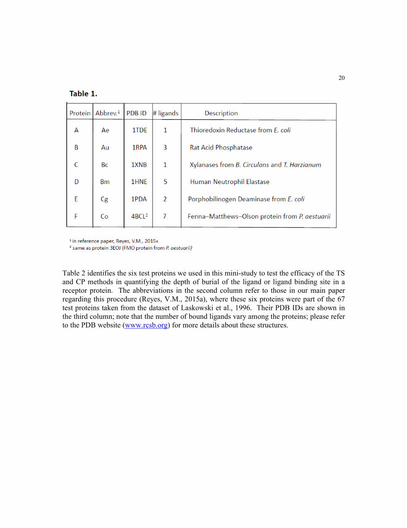
the Laskowski et al. dataset (1996) that were tested in this small pilot study. Protein A, (PDB ID: 1TDE),

thioredoxin reductase from E. coli, has a single bound ligand, FAD-500. Protein B, (PDB ID: 1RPA), rat acid

phosphatase, has three ligands, namely, TAR-343, NAG-344 and NAG-347. Protein C, (PDB ID: 1XNB),

xylanase from B. circulans/T. harzianum, also has a single ligand, S04-191. Protein D, (PDB ID: 1HNE), human

neutrophil elastase, has five ligands, which are ALM I-5, MSU I-1, ALA I-2, ALA I-3 and PRO I-4. Protein E,

(PDB ID: 1PDA), phorphobilinogen from E. coli, has two ligands, DPM-314 and ACY-315. Finally, protein F,

(PDB ID: 4BCL a.k.a. 3EOJ), FMO protein from P. aestuarii has seven ligands, namely, BCL-1, BCL-2, BCL-

3, BCL-4, BCL-5, BCL-6 and BCL-7.

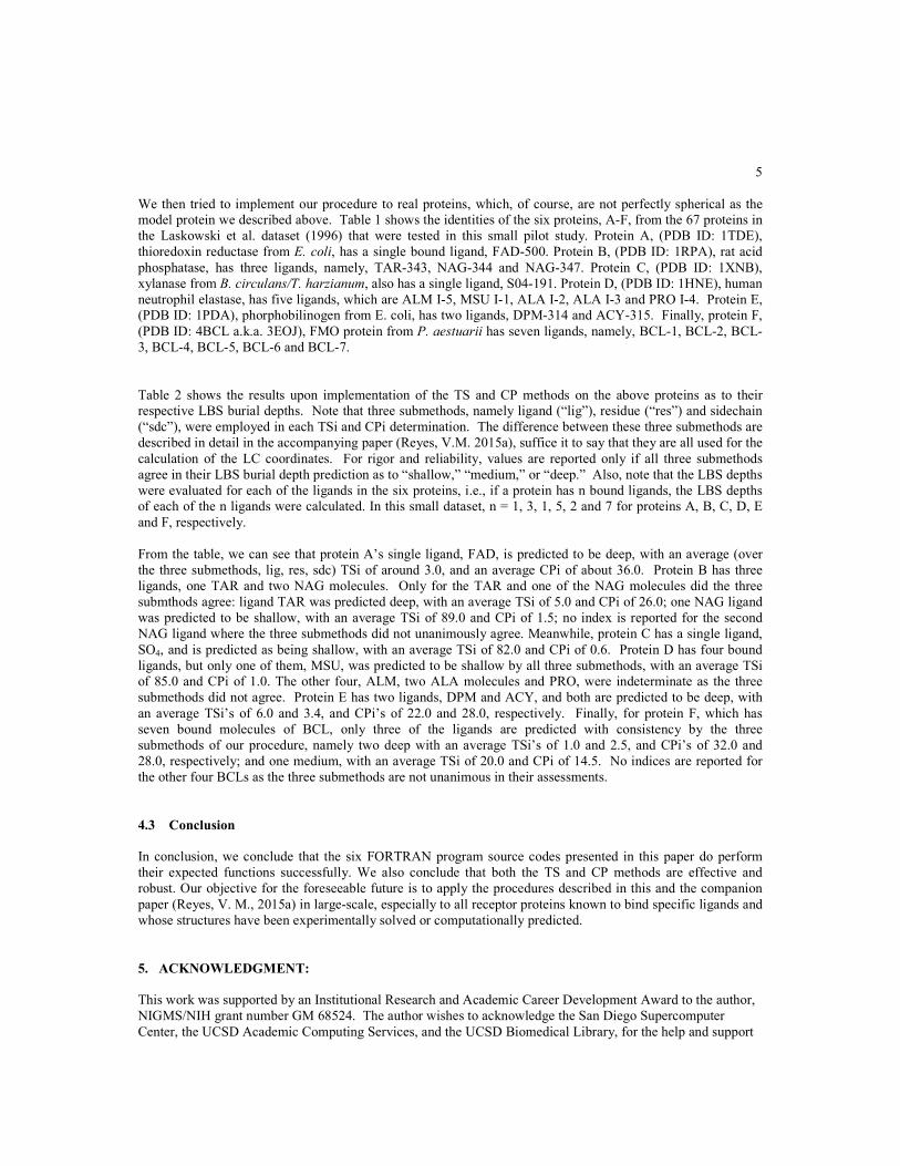
Table 2 shows the results upon implementation of the TS and CP methods on the above proteins as to their

respective LBS burial depths. Note that three submethods, namely ligand (“lig”), residue (“res”) and sidechain

(“sdc”), were employed in each TSi and CPi determination. The difference between these three submethods are

described in detail in the accompanying paper (Reyes, V.M. 2015a), suffice it to say that they are all used for the

calculation of the LC coordinates. For rigor and reliability, values are reported only if all three submethods

agree in their LBS burial depth prediction as to “shallow,” “medium,” or “deep.” Also, note that the LBS depths

were evaluated for each of the ligands in the six proteins, i.e., if a protein has n bound ligands, the LBS depths

of each of the n ligands were calculated. In this small dataset, n = 1, 3, 1, 5, 2 and 7 for proteins A, B, C, D, E

and F, respectively.

From the table, we can see that protein A’s single ligand, FAD, is predicted to be deep, with an average (over

the three submethods, lig, res, sdc) TSi of around 3.0, and an average CPi of about 36.0. Protein B has three

ligands, one TAR and two NAG molecules. Only for the TAR and one of the NAG molecules did the three

submthods agree: ligand TAR was predicted deep, with an average TSi of 5.0 and CPi of 26.0; one NAG ligand

was predicted to be shallow, with an average TSi of 89.0 and CPi of 1.5; no index is reported for the second

NAG ligand where the three submethods did not unanimously agree. Meanwhile, protein C has a single ligand,

SO4, and is predicted as being shallow, with an average TSi of 82.0 and CPi of 0.6. Protein D has four bound

ligands, but only one of them, MSU, was predicted to be shallow by all three submethods, with an average TSi

of 85.0 and CPi of 1.0. The other four, ALM, two ALA molecules and PRO, were indeterminate as the three

submethods did not agree. Protein E has two ligands, DPM and ACY, and both are predicted to be deep, with

an average TSi’s of 6.0 and 3.4, and CPi’s of 22.0 and 28.0, respectively. Finally, for protein F, which has

seven bound molecules of BCL, only three of the ligands are predicted with consistency by the three

submethods of our procedure, namely two deep with an average TSi’s of 1.0 and 2.5, and CPi’s of 32.0 and

28.0, respectively; and one medium, with an average TSi of 20.0 and CPi of 14.5. No indices are reported for

the other four BCLs as the three submethods are not unanimous in their assessments.

4.3 Conclusion

In conclusion, we conclude that the six FORTRAN program source codes presented in this paper do perform

their expected functions successfully. We also conclude that both the TS and CP methods are effective and

robust. Our objective for the foreseeable future is to apply the procedures described in this and the companion

paper (Reyes, V. M., 2015a) in large-scale, especially to all receptor proteins known to bind specific ligands and

whose structures have been experimentally solved or computationally predicted.

5. ACKNOWLEDGMENT:

This work was supported by an Institutional Research and Academic Career Development Award to the author,

NIGMS/NIH grant number GM 68524. The author wishes to acknowledge the San Diego Supercomputer

Center, the UCSD Academic Computing Services, and the UCSD Biomedical Library, for the help and support

6

of their staff and personnel. He also acknowledges the Division of Research Computing at RIT, and computing

resources from the Dept. of Biological Sciences, College of Science, at RIT.

6. REFERENCES:

Anderson, G. and Anderson, P. (1986), The Unix C Shell Field Guide, Prentice Hall (Publ.)

Aho, A.V., Kernighan, B.W. & Weinberger, P.J. (1988) The AWK Programming Language, Pearson (Publ.)

Ben-Shimon, A., and Eisenstein, M. (2005). Looking at enzymes from the inside out: the proximity of

catalytic residues to the molecular centroid can be used for detection of active sites and enzyme-ligand

interfaces. J Mol Biol. 351:309-26.

Berman, J.J. (2007) Perl Programming for Medicine and Biology (Series in Biomedical Informatics),

Jones & Bartlett (Publ.)

Berman, H.M., Westbrook, J., Feng, Z., Gilliland, G., Bhat, T.N., Weissig, H., Shindyalov, I.N., Bourne, P.E.

(2000) The Protein Data Bank, Nucleic Acids Research, 28: 235-242. (URL: www.rcsb.org)

Birns, P., Brown, P., Muster, J.C.C. (1985 ) UNIX for People, Prentice Hall (Publ.)

Chapman, S.J. (1997) FORTRAN 90/95 for Scientists and Engineers, McGraw-Hill Science/Engineering/Math

(Publ.)

Cheguri, S. and Reyes, V.M. (2011) “A Database/Webserver for Size-Independent Quantification of Ligand

Binding Site Burial Depth in Receptor Proteins: Implications on Protein Dynamics”, J. Biomol. Struct. & Dyn.,

Book of Abstracts, Albany: The 17th Conversation, June 14-18, 2011, Vol. 28 (6) June 2011, p. 1013

Dougherty, D. and Robbins, A. (1997), Sed & Awk (2nd Ed.), O'Reilly Media (Publ.)

Holoien, M.O., Behforooz, A. (1991) Fortran 77 for Engineers and Scientists (2nd Ed.), Brooks/Cole Pub Co.

(Publ.)

Mayo, W., Cwiakala, M. (1994) Schaum's Outline of Programming With Fortran 77 (Schaum's Outlines),

McGraw-Hill Education (Publ.)

Metcalf, M. and Reid, J.K. (1999) Fortran 90/95 Explained (2nd Ed.), Oxford University Press (Publ.)

Nyhoff, L. and Leestma, S. (1996) FORTRAN 77 for Engineers and Scientists with an Introduction to

FORTRAN 90 (4th Ed.), Pearson (Publ.)

Nyhoff, L. and Leestma, S. (1996) FORTRAN 90 for Engineers and Scientists, Pearson (Publ.)

Nyhoff, L. and Leestma, S. (1999) Introduction to FORTRAN 90, ESource Series (2nd Ed.), Prentice Hall

(Publ.)

Powers, S., Peek, J., O'Reilly, T., Loukides, M. (2002), Unix Power Tools (3rd Ed.), O'Reilly Media (Publ.)

Reyes, V.M. (2015a) "Two Complementary Methods for Relative Quantification of Ligand Binding Site Burial

Depth in Proteins: The ‘Cutting Plane’ and ‘Tangent Sphere’ Methods" [e-pub ahead of publication:

arXiv.org/abs/1505.01142 [Quantitative Biology: Biomolecules]]

7

Reyes, V.M. & Sheth, V.N. (2011) "Visualization of Protein 3D Structures in 'Double-Centroid' Reduced

Representation: Application to Ligand Binding Site Modeling and Screening" (2011), Handbook of Research in

Computational and Systems Biology: Interdisciplinary Approaches, IGI-Global/Springer, pp. 583-598

Reyes, V.M. (2015b) “An Automatable Analytical Algorithm for Structure-Based Protein Functional

Annotation via Detection of Specific Ligand 3D Binding Sites: Application to ATP (ser/thr Protein Kinases) and

GTP (Small Ras–type G-Proteins) Binding Sites” [e-pub ahead of publication: arXiv.org/abs/1505.01141

[Quantitative Biology: Biomolecules]]

Reyes, V.M. (2015c) “Structure-Based Function Prediction of Functionally Unannotated Structures in the PDB:

Prediction of ATP, GTP, Sialic Acid, Retinoic Acid and Heme-bound and -Unbound (Free) Nitric Oxide Protein

Binding Sites.” [e-pub ahead of publication: arXiv.org/abs/1505.01143 [Quantitative Biology: Biomolecules]]

Reyes, V.M. (2015d) “A Global and Local Structure-Based Method for Predicting Binary Protein-Protein

Interaction Partners: Proof of Principle and Feasibility.” [e-pub ahead of publication: arXiv.org/abs/1505.01144

[Quantitative Biology: Biomolecules]]

Tisdall, J. (2001) Beginning Perl for Bioinformatics 1st Edition, O'Reilly Media (Publ.)

8. FIGURES and LEGENDS:

----------------------------------------------------------------------------------------------------------------------------------- Figure 1: ..... page 18 Figure 2: ..... page 19

-----------------------------------------------------------------------------------------------------------------------------------

9. TABLES and LEGENDS:

-----------------------------------------------------------------------------------------------------------------------------------

Table 1: ..... page 20 Table 2: ..... page 21

-----------------------------------------------------------------------------------------------------------------------------------

9. PROGRAMS:

Program 1:

########## Start of Pogram “find_molec_centr.f” ##########

program find_molecular_centroid ! c c c c c c c c c c c c c c c c c c c c c c c c c c c c c c c c c c c c ! c

8

! Author: Vicente M. Reyes, Ph.D. c ! Dept. of Pharmacol., Skaggs Sch. of Pharm. & Pharm. Sci. c ! & Dept. of Integrative Biosci., S.D. Supercomptr. Ctr. c ! La Jolla, CA 92093-0505 U.S.A. c ! c ! c c c c c c c c c c c c c c c c c c c c c c c c c c c c c c c c c c c c character*30 left character*30 right integer count real x, y, z, sum_x, sum_y, sum_z, xc, yc, zc open (unit =1, file = "filei") open (unit =2, file = "fileo") count = 0 sum_x = 0.00 sum_y = 0.00 sum_z = 0.00 888 read(1,100,end=333) left, x, y, z, right 100 format(A30, f8.3, f8.3, f8.3, A30) count = count + 1 sum_x = sum_x + x sum_y = sum_y + y sum_z = sum_z + z go to 888 333 continue xc = sum_x/count yc = sum_y/count zc = sum_z/count write (2,200) xc, yc, zc 200 format(f10.5, f10.5, f10.5) ! print*, "x = ", xc ! print*, "y = ", yc ! print*, "z = ", zc close(2) close(1) stop end

########## End of Pogram “find_molec_centr.f” ##########

Program 2:

########## Start of Pogram “tangent_sphere.f” ##########

9

c program: tangent_sphere.f c c c c c c c c c c c c c c c c c c c c c c c c c c c c c c c c c c c c c c c c Author: Vicente M. Reyes, Ph.D. c c Dept. of Pharmacol., Skaggs Sch. of Pharm. & Pharm. Sci. c c & Dept. of Integrative Biosci., S.D. Supercomptr. Ctr. c c La Jolla, CA 92093-0505 U.S.A. c c c c c c c c c c c c c c c c c c c c c c c c c c c c c c c c c c c c c c c c character*30 left character*22 mesg character*5 lbl1,lbl2,lbl3,lbl4,lbl5,lbl6,lbl7,lbl8 real count, inside, outside, pct_in, pct_out real xc, yc, zc , xp, yp, zp, radius, dist ! input files: open (unit =1, file = "filea") ! <-- center of sphere: x,y,z: ??.prot.CM open (unit =2, file = "fileb") ! <-- radius of sphere: ??.lbs?.prot.CM.len open (unit =3, file = "filec") ! <-- pdb file of protein under test: ??.prot ! output file: open (unit =4, file = "filew") ! <-- atoms inside sphere open (unit =5, file = "filex") ! <-- atoms outside sphere open (unit =6, file = "filey") ! <-- atoms right on sphere open (unit =7, file = "filez") ! <-- results: %in, %out, %on count = 0.0 inside = 0.0 outside = 0.0 righton = 0.0 lbl1 = 'dist=' lbl2 = '%in= ' lbl3 = '#in= ' lbl4 = '%out=' lbl5 = '#out=' lbl6 = '%on= ' lbl7 = '#on= ' lbl8 = 'Tot= ' mesg = "point right on sphere!" 888 read(1,100) xc, yc, zc 100 format (f10.5, f10.5, f10.5) read(2,200) radius 200 format (f10.5) 999 read(3,300,end=444) left, xp, yp, zp 300 format(A30, f8.3, f8.3, f8.3) count = count + 1.0 dist = sqrt((xc-xp)**2 + (yc-yp)**2 + (zc-zp)**2) if(dist.lt.radius) then

10

write(4,400) left, xp, yp, zp, lbl1, dist inside = inside + 1.0 elseif (dist.gt.radius) then write(5,400) left, xp, yp, zp, lbl1, dist outside = outside + 1.0 else write(6,401) left, xp, yp, zp, lbl1, dist, mesg righton = righton + 1.0 400 format(A30, f8.3, f8.3, f8.3, 3x, A5, f10.5) 401 format(A30, f8.3, f8.3, f8.3, 3x, A5, f10.5, 3x, A16) endif go to 999 444 pct_in = (inside/count)*100.0 pct_out = (outside/count)*100.0 pct_on = (righton/count)*100.0 write(7,700) lbl2,pct_in, lbl3,inside, lbl4,pct_out, + lbl5,outside, lbl6,pct_on, lbl7,righton, lbl8,count 700 format (A5, f9.3, 3x, A5,f9.0, 3x, A5,f9.3, 3x, A5, + f9.0, 3x, A5,f5.3, 3x, A5,f4.0, 3x, A5,f9.0) brodie:/home/vmrsbi/projects/TSM.theoret (378) % c TSM.f c program: tangent_sphere.f character*30 left character*22 mesg character*5 lbl1,lbl2,lbl3,lbl4,lbl5,lbl6,lbl7,lbl8 real count, inside, outside, pct_in, pct_out real xc, yc, zc , xp, yp, zp, radius, dist ! input files: open (unit =1, file = "filea") ! <-- center of sphere: x,y,z: ??.prot.CM open (unit =2, file = "fileb") ! <-- radius of sphere: ??.lbs?.prot.CM.len open (unit =3, file = "filec") ! <-- pdb file of protein under test: ??.prot ! output file: open (unit =4, file = "filew") ! <-- atoms inside sphere open (unit =5, file = "filex") ! <-- atoms outside sphere open (unit =6, file = "filey") ! <-- atoms right on sphere open (unit =7, file = "filez") ! <-- results: %in, %out, %on count = 0.0 inside = 0.0 outside = 0.0 righton = 0.0 lbl1 = 'dist=' lbl2 = '%in= ' lbl3 = '#in= ' lbl4 = '%out=' lbl5 = '#out='

11

lbl6 = '%on= ' lbl7 = '#on= ' lbl8 = 'Tot= ' mesg = "point right on sphere!" 888 read(1,100) xc, yc, zc 100 format (f10.5, f10.5, f10.5) read(2,200) radius 200 format (f10.5) 999 read(3,300,end=444) left, xp, yp, zp 300 format(A30, f8.3, f8.3, f8.3) count = count + 1.0 dist = sqrt((xc-xp)**2 + (yc-yp)**2 + (zc-zp)**2) if(dist.lt.radius) then write(4,400) left, xp, yp, zp, lbl1, dist inside = inside + 1.0 elseif (dist.gt.radius) then write(5,400) left, xp, yp, zp, lbl1, dist outside = outside + 1.0 else write(6,401) left, xp, yp, zp, lbl1, dist, mesg righton = righton + 1.0 400 format(A30, f8.3, f8.3, f8.3, 3x, A5, f10.5) 401 format(A30, f8.3, f8.3, f8.3, 3x, A5, f10.5, 3x, A16) endif go to 999 444 pct_in = (inside/count)*100.0 pct_out = (outside/count)*100.0 pct_on = (righton/count)*100.0 write(7,700) lbl2,pct_in, lbl3,inside, lbl4,pct_out, + lbl5,outside, lbl6,pct_on, lbl7,righton, lbl8,count 700 format (A5, f9.3, 3x, A5,f9.0, 3x, A5,f9.3, 3x, A5, + f9.0, 3x, A5,f5.3, 3x, A5,f4.0, 3x, A5,f9.0) close(7) close(6) close(5) close(4) close(3) close(2) close(1) stop

12

end

########## End of Pogram “tangent_sphere.f” ##########

Program 3:

########## Start of Pogram “find_CP_coeffs.f” ########## c program find_CP_coeffs.f c c c c c c c c c c c c c c c c c c c c c c c c c c c c c c c c c c c c c c c c Author: Vicente M. Reyes, Ph.D. c c Dept. of Pharmacol., Skaggs Sch. of Pharm. & Pharm. Sci. c c & Dept. of Integrative Biosci., S.D. Supercomptr. Ctr. c c La Jolla, CA 92093-0505 U.S.A. c c c c c c c c c c c c c c c c c c c c c c c c c c c c c c c c c c c c c c c c c see ~/science_notes, lines 2515 ff character*45 n_mesg, p_mesg, z_mesg real p,q,r,s,t,u real A,B,C,D,val open (unit =1, file = "filea") !this is point #1, lbs?.CM open (unit =2, file = "fileb") !this is point #2, prot.CM open (unit =3, file = "fileo") !output file: prot CM on pos. side of CP p_mesg = 'gCM on (+) side of CP => external side is (-)' n_mesg = 'gCM on (-) side of CP => coeff signs reversed' z_mesg = 'gCM lies right on the CP!! A very rare case!!' 888 read(1,100) p, q, r ! this is P1: lbs.CM == local CM 999 read(2,100) s, t, u ! this is P2: prot.CM == global CM 100 format(f10.5, f10.5, f10.5) !******************************************************************* ! complex in question; i.e., L = (p,q,r) = local CM and ! G = (s,t,u) = global CM ! Q = (x,y,z) = any point on the cutting plane, CP ! ! ! The equation of the plane is then: Ax + By + Cz + D = 0 ! ! where A = s-p ! B = t-q ! C = u-r ! and D = p(p-s) + q(q-t) + r(r-u) QED ! ! NOTE: The prot CM (global CM) is always on the positive side of the CP and

13

! thus the exteternal side of the CP is alweays its negative side!!!!!!! ! !******************************************************************* A = s-p B = t-q C = u-r D = ((p*(p-s)) + (q*(q-t)) + (r*(r-u))) val = A*s + B*t + C*u + D !!! it can be shown that "val" is always (+) if (val.gt.(0.0)) then write(3,300) A,B,C,D,p_mesg, val 300 format(f12.5, f12.5, f12.5, f12.5, 3x, A45, f10.3) elseif (val.lt.(0.0)) then write(3,300) -A,-B,-C,-D,n_mesg, -val elseif (val.eq.(0.0)) then write(3,300) A,B,C,D,z_mesg, val endif 333 continue close(3) close(2) close(1) stop end

########## End of Pogram “find_CP_coeffs.f” ##########

Program 4:

########## Start of Pogram “CPM_Neg_Side.f “ ##########

c program: CPM_NegSid.f c c c c c c c c c c c c c c c c c c c c c c c c c c c c c c c c c c c c c c c c Author: Vicente M. Reyes, Ph.D. c c Dept. of Pharmacol., Skaggs Sch. of Pharm. & Pharm. Sci. c c & Dept. of Integrative Biosci., S.D. Supercomptr. Ctr. c c La Jolla, CA 92093-0505 U.S.A. c c c c c c c c c c c c c c c c c c c c c c c c c c c c c c c c c c c c c c c c character*30 left character*5 lbl1, lbl4, lbl5, lbl8 real numneg, pct_neg, val

14

real A, B, C, D, x, y, z, total ! input files: open (unit =1, file = "filea") ! <-- CP coeffs: ??.lbs?.CP_coeffs open (unit =2, file = "fileb") ! <-- pdb file of protein under test: ??.prot ! output file: open (unit =4, file = "filey") ! <-- prot atoms on (-) side of CP open (unit =5, file = "filez") ! <-- results: %(-), #(-) total = 0.0 numneg = 0.0 lbl1 = 'val= ' lbl4 = '%(-)=' lbl5 = '#(-)=' lbl8 = 'Tot= ' 888 read(1,100) A,B,C,D 100 format(f12.5, f12.5, f12.5, f12.5) 999 read(2,300,end=444) left, x, y, z 300 format(A30, f8.3, f8.3, f8.3) total = total + 1.0 val = A*x + B*y + C*z + D if (val.lt.(0.0)) then write(4,400) left, x, y, z, lbl1, val numneg = numneg + 1.0 400 format(A30, f8.3, f8.3, f8.3, 3x, A5, f10.5) endif go to 999 444 pct_neg = (numneg/total)*100.0 write(5,500)lbl4,pct_neg, lbl5,numneg, lbl8,total 500 format(A5,f10.4, 3x, A5,f10.0, 3x, A5,f10.0) close(5) close(4) close(2) close(1) stop end

########## End of Pogram “CPM_Neg_Side.f” ##########

15

Program 5:

########## Start of Pogram “CPM_Pos_Side.f” ##########

c program: CPM_PosSid.f c c c c c c c c c c c c c c c c c c c c c c c c c c c c c c c c c c c c c c c c Author: Vicente M. Reyes, Ph.D. c c Dept. of Pharmacol., Skaggs Sch. of Pharm. & Pharm. Sci. c c & Dept. of Integrative Biosci., S.D. Supercomptr. Ctr. c c La Jolla, CA 92093-0505 U.S.A. c c c c c c c c c c c c c c c c c c c c c c c c c c c c c c c c c c c c c c c c character*30 left character*5 lbl1, lbl2, lbl3, lbl8 real numpos, pct_pos, val real A, B, C, D, x, y, z, total ! input files: open (unit =1, file = "filea") ! <-- CP coeffs: ??.lbs?.CP_coeffs open (unit =2, file = "fileb") ! <-- pdb file of protein under test: ??.prot ! output file: open (unit =3, file = "filex") ! <-- prot atoms on (+) side of CP open (unit =5, file = "filez") ! <-- results: %(+), #(+) total = 0.0 numpos = 0.0 lbl1 = 'val= ' lbl2 = '%(+)=' lbl3 = '#(+)=' lbl8 = 'Tot= ' 888 read(1,100) A,B,C,D 100 format(f12.5, f12.5, f12.5, f12.5) 999 read(2,300,end=444) left, x, y, z 300 format(A30, f8.3, f8.3, f8.3) total = total + 1.0 val = A*x + B*y + C*z + D if (val.gt.(0.0)) then write(3,400) left, x, y, z, lbl1, val numpos = numpos + 1.0 400 format(A30, f8.3, f8.3, f8.3, 3x, A5, f10.5) endif go to 999

16

444 pct_pos = (numpos/total)*100.0 write(5,500)lbl2,pct_pos, lbl3,numpos, lbl8,total 500 format(A5,f10.4, 3x, A5,f10.0, 3x, A5,f10.0) close(5) close(3) close(2) close(1) stop end

########## End of Pogram “CPM_Pos_Side.f” ##########

Program 6:

########## Start of Pogram “CPM_Zero_Side.f” ##########

c program: CPM_ZerSid.f c c c c c c c c c c c c c c c c c c c c c c c c c c c c c c c c c c c c c c c c Author: Vicente M. Reyes, Ph.D. c c Dept. of Pharmacol., Skaggs Sch. of Pharm. & Pharm. Sci. c c & Dept. of Integrative Biosci., S.D. Supercomptr. Ctr. c c La Jolla, CA 92093-0505 U.S.A. c c c c c c c c c c c c c c c c c c c c c c c c c c c c c c c c c c c c c c c c character*30 left character*5 lbl1, lbl6, lbl7, lbl8 real numzer, pct_zer, val real A, B, C, D, x, y, z, total ! input files: open (unit =1, file = "filea") ! <-- CP coeffs: ??.lbs?.CP_coeffs open (unit =2, file = "fileb") ! <-- pdb file of protein under test: ??.prot ! output file: open (unit =3, file = "filex") ! <-- prot atoms on (0) side of CP open (unit =5, file = "filez") ! <-- results: %(0), #(0), total = 0.0 numzer = 0.0 lbl1 = 'val= ' lbl6 = '%(0)=' lbl7 = '#(0)=' lbl8 = 'Tot= ' 888 read(1,100) A,B,C,D 100 format(f12.5, f12.5, f12.5, f12.5) 999 read(2,300,end=444) left, x, y, z

17

300 format(A30, f8.3, f8.3, f8.3) total = total + 1.0 val = A*x + B*y + C*z + D if (val.eq.(0.0)) then write(3,400) left, x, y, z, lbl1, val numzer = numzer + 1.0 400 format(A30, f8.3, f8.3, f8.3, 3x, A5, f10.5) endif go to 999 444 pct_zer = (numzer/total)*100.0 write(5,500)lbl6,numzer, lbl7,pct_zer, lbl8,total 500 format(A5,f10.4, 3x, A5,f10.0, 3x, A5,f10.0) close(5) close(3) close(2) close(1) stop end

########## End of Pogram “CPM_Zero_Side.f” ##########

18

10. FIGURES:

Figure 1 illustrates the concept behind the Tangent Sphere and Cutting Plane methods. A

hypothetical protein is represented by a collection of black dots collectively forming a sphere;

the tangent sphere (TS) is represented by the red circle, whose center is the protein’s centroid;

the cutting plane (CP) is represented by the blue line, which is tangent to the TS at the ligand

binding site (LBS). As the LBS gets deeper (from left to right), the volume of the TS

decreases, while the portion of the protein cut off by the CP increases. The TSA index (TSi)

is the number of protein atoms inside the TS, while the CP index (CPi) is the number of

protein atoms cut off by the CP.

19

On The plots on the left panel in Figure 2 refer to the theoretical (a.k.a. model) protein shown

schematically on the right. The model protein is a three-dimensional grid of points that

collectively form a sphere with center at (0,0,0,) and radius 50 units, and separated by equal

distances of 1.5 units along the x-, y- and z-directions. The LBS opening is designated to be

at the “north pole” of the sphere, i.e., at (0,0,50). The horizontal axis of the plot in the left

panel represent the distance from the LBS along the z-axis, and the vertical axis represent

percentages of protein atoms that are either inside the TS (blue curve) or cut off (intercepted,

or on the external side of) by the CP (red curve). If the LBS opening (from which the ligand

‘enters’ the protein LBS) is not considered (as in real cases, since this information is usually

unknown, or unamenable to batch-mode computation) only the left half of the blue+red

curves will be displayed, but with double the number of data points (because the right half of

the blue+red curves would have “folded into” the left half. These are the green curve and

maroon curves, for the TS and CP methods, respectively.

11. TABLES:

20

Table 2 identifies the six test proteins we used in this mini-study to test the efficacy of the TS

and CP methods in quantifying the depth of burial of the ligand or ligand binding site in a

receptor protein. The abbreviations in the second column refer to those in our main paper

regarding this procedure (Reyes, V.M., 2015a), where these six proteins were part of the 67

test proteins taken from the dataset of Laskowski et al., 1996. Their PDB IDs are shown in

the third column; note that the number of bound ligands vary among the proteins; please refer

to the PDB website (www.rcsb.org) for more details about these structures.

21

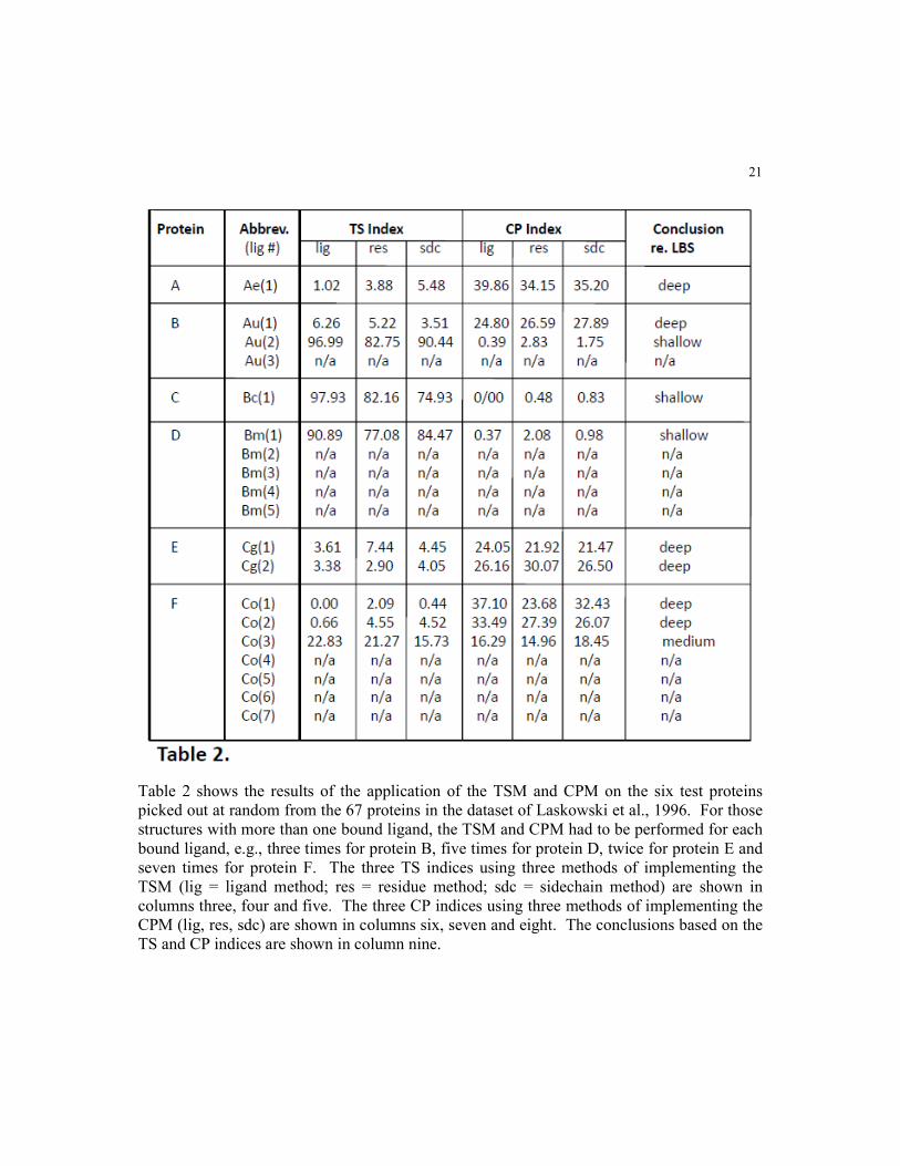
Table 2 shows the results of the application of the TSM and CPM on the six test proteins

picked out at random from the 67 proteins in the dataset of Laskowski et al., 1996. For those

structures with more than one bound ligand, the TSM and CPM had to be performed for each

bound ligand, e.g., three times for protein B, five times for protein D, twice for protein E and

seven times for protein F. The three TS indices using three methods of implementing the

TSM (lig = ligand method; res = residue method; sdc = sidechain method) are shown in

columns three, four and five. The three CP indices using three methods of implementing the

CPM (lig, res, sdc) are shown in columns six, seven and eight. The conclusions based on the

TS and CP indices are shown in column nine.