Embed Size (px)
Citation preview
hep-th/0305188
Superconformal D-branesand moduli spaces
Cecilia Albertsson
Doctoral Thesis inTheoretical Physics
Department of PhysicsStockholm University
2003
Thesis for the degree of doctor of philosophy in theoretical physicsDepartment of Physics, Stockholm UniversitySweden
c© Cecilia Albertsson 2003ISBN 91-7265-630-1 (pp i-ix, 1-64)Akademitryck AB, Edsbruk
Abstract
The on-going quest for a single theory that describes all the forces ofnature has led to the discovery of string theory. This is the only knowntheory that successfully unifies gravity with the electroweak and strongforces. It postulates that the fundamental building blocks of nature arestrings, and that all particles arise as different excitations of strings.This theory is still poorly understood, especially at strong coupling,but progress is being made all the time. One breakthrough came withthe discovery of extended objects called D-branes, which have provedcrucial in probing the strong-coupling regime. They are instrumental inrealising dualities (equivalences) between different limits of string theory.
This thesis is concerned with dualities and D-branes. First, it givesa background and review of the first article, where we substantiated aconjectured duality between two a priori unrelated gauge theories. Thesegauge theories have different realisations as the worldvolume theories ondifferent D-brane configurations. We showed that there is an identitybetween the spaces of vacua (moduli spaces) arising in the two theories,which suggests that the corresponding string theory pictures are dual.
Second, we give a background and description of the analysis per-formed in the remaining three articles, where we derived the most gen-eral, local, superconformal boundary conditions of the two-dimensionalnonlinear sigma model. This model describes the dynamics of openstrings, and the boundary conditions dictate the geometry of D-branes.In the last article we studied these boundary conditions for the specialcase of WZW models.
Acknowledgements
First and foremost, I am immensely indebted to my advisor Ulf Lind-strom, without whose help and guidance this thesis could never havecome into being. He has always devoted ample time to answering myquestions and discussing problems whenever I needed to, often at a meremoment’s notice. I feel he always took great interest in my progress, andoffered lots of support and encouragement, especially at times when Ireally needed it.
I have also greatly enjoyed working with both Bjorn Brinne andMaxim Zabzine. It has been very stimulating, and their enthusiasm forsolving the mysteries of string theory is infectious to say the least. Inaddition they contributed to a social and relaxed atmosphere during myfirst two years in Stockholm, as did Tasneem Zehra Husain, who alsoadded colour and joy to our office in the new building.
Thanks also to Ron Reid-Edwards for providing the office entertain-ment during my stay at Queen Mary, and to all the other people therewho made my visit an enjoyable one.
Ansar Fayyazuddin deserves special thanks for being the drivingforce behind the study group, which I found incredibly useful, as doesIngemar Bengtsson for encouraging me to apply to Fysikum in the firstplace.
Last, but certainly not least, my eternal gratitude goes to mom anddad for always believing in me, and for their unfailing support throughdifficult times, well beyond the call of parental duty, by any definition.

For Fay,
who brightened my life
for fifteen wonderful years

Contents
1 Introduction 11.1 Strings . . . . . . . . . . . . . . . . . . . . . . . . . . . . . 21.2 D-branes . . . . . . . . . . . . . . . . . . . . . . . . . . . . 31.3 Outline . . . . . . . . . . . . . . . . . . . . . . . . . . . . 41.4 About the thesis . . . . . . . . . . . . . . . . . . . . . . . 5
2 Moduli spaces 72.1 Introduction . . . . . . . . . . . . . . . . . . . . . . . . . . 7
2.1.1 Mirror symmetry . . . . . . . . . . . . . . . . . . . 82.1.2 Outline . . . . . . . . . . . . . . . . . . . . . . . . 9
2.2 Lie algebras . . . . . . . . . . . . . . . . . . . . . . . . . . 102.2.1 Definitions . . . . . . . . . . . . . . . . . . . . . . 102.2.2 Finding the roots . . . . . . . . . . . . . . . . . . . 112.2.3 Dynkin diagrams . . . . . . . . . . . . . . . . . . . 13
2.3 N=2 super-Yang-Mills theory . . . . . . . . . . . . . . . . 132.3.1 Defining our SYM theory . . . . . . . . . . . . . . 142.3.2 Spontaneous symmetry breaking . . . . . . . . . . 162.3.3 The N=2 potential . . . . . . . . . . . . . . . . . . 192.3.4 The SYM moduli space . . . . . . . . . . . . . . . 212.3.5 Singularities . . . . . . . . . . . . . . . . . . . . . . 222.3.6 Nonzero FI-terms . . . . . . . . . . . . . . . . . . . 23
2.4 Seiberg-Witten theory . . . . . . . . . . . . . . . . . . . . 242.4.1 Elliptic fibrations . . . . . . . . . . . . . . . . . . . 252.4.2 Connection to physics . . . . . . . . . . . . . . . . 26
2.4.3 Brane picture . . . . . . . . . . . . . . . . . . . . . 272.5 Quiver gauge theory . . . . . . . . . . . . . . . . . . . . . 29
2.5.1 Effects of orbifolding . . . . . . . . . . . . . . . . . 302.5.2 Quiver diagrams . . . . . . . . . . . . . . . . . . . 33
2.6 The N=2 Higgs branch . . . . . . . . . . . . . . . . . . . 342.6.1 Comparing the moduli spaces . . . . . . . . . . . . 35
3 Boundary conditions 373.1 Introduction . . . . . . . . . . . . . . . . . . . . . . . . . . 37
3.1.1 Outline . . . . . . . . . . . . . . . . . . . . . . . . 393.2 The bosonic model . . . . . . . . . . . . . . . . . . . . . . 39
3.2.1 Conserved currents . . . . . . . . . . . . . . . . . . 403.3 The superspace action . . . . . . . . . . . . . . . . . . . . 42
3.3.1 Finding the currents . . . . . . . . . . . . . . . . . 433.4 The ansatz . . . . . . . . . . . . . . . . . . . . . . . . . . 443.5 Structures on D-branes . . . . . . . . . . . . . . . . . . . . 463.6 The boundary conditions . . . . . . . . . . . . . . . . . . 493.7 Globally defined conditions . . . . . . . . . . . . . . . . . 51
3.7.1 Examples . . . . . . . . . . . . . . . . . . . . . . . 523.8 The WZW model . . . . . . . . . . . . . . . . . . . . . . . 53
3.8.1 Symmetries . . . . . . . . . . . . . . . . . . . . . . 543.8.2 The gluing map . . . . . . . . . . . . . . . . . . . . 55
Bibliography 59
Accompanying papers
I: E8 Quiver Gauge Theory and Mirror Symmetry,C. Albertsson, B. Brinne, U. Lindstrom and R. von Unge,JHEP 05 (2001) 021, hep-th/0102038.
II: N = 1 supersymmetric nonlinear sigma model with boundaries, I,C. Albertsson, U. Lindstrom and M. Zabzine,Commun. Math. Phys. 233 (2003) 3, 403-421, hep-th/0111161.
III: N = 1 supersymmetric nonlinear sigma model with boundaries, II,C. Albertsson, U. Lindstrom and M. Zabzine,submitted to Commun. Math. Phys. (2002), hep-th/0202069.
IV: Superconformal boundary conditions for the WZW model,C. Albertsson, U. Lindstrom and M. Zabzine,JHEP 05 (2003) 050, preprint no. UUITP-05-03, USITP-2003-02,hep-th/0304013.

Chapter 1
Introduction
“This sort of thing has cropped up before,and it has always been due to human error.”
— HAL 9000, in 2001: A Space Odyssey
Although the film’s supercomputer was referring to a faulty com-munications device, its statement turned out to carry universal truth,much to the dismay of the ill-fated crew of Discovery. And not only wasthe fault indeed induced by humans, it was of a fundamentally differentnature than the crew initially thought.
This is characteristic of research in theoretical physics. The questfor an ultimate theory that will explain all the forces of nature in asingle, beautiful principle, is a typically human one. Besides a curiosityabout the world around us, we are driven by our desire for aesthetics andsimplicity. Sometimes so much so that we are tempted to make over-simplified assumptions about nature, such as the Aristotelian “naturalstate,” or Copernicus’ circular planetary orbits. We may be unaware ofthe error, building entire theories on our flawed axioms, and not untildisaster strikes do we realise just how fundamental a mistake we havemade.
1
2 CHAPTER 1. INTRODUCTION
It is easy to make such mistakes because nature often turns out to bemuch more peculiar than we ever imagined, displaying counterintuitiveeffects like the particle-wave duality. At first, such weirdness might bemisconstrued as complications. But going along with it usually in theend leads to an even simpler picture of the world, bringing us closer toa unified theory of everything. So as a physicist, one learns to acceptridiculous ideas just for the sake of argument.
One such “ridiculous idea” constitutes the foundation of string the-ory.
1.1 Strings
The idea is that all elementary particles are actually vibrating strings.This was put forward by phycisists in the seventies, after failing to
use string theory to describe the strong interactions (quantum chromo-dynamics does a better job of that). It was realised that string theoryunifies gravity with the three forces described by quantum field theory— electromagnetism, the weak force and the strong force. Because thebasic building blocks are one-dimensional objects, strings, instead ofzero-dimensional point particles, string theory does not suffer from thedivergences of quantum field theory.
The fact that strings are one-dimensional leads to a vast range ofpossible string states. Strings can be open (two ends) or closed (endsjoined), and they can oscillate in a multitude of ways. The differentstates that arise in this way correspond to different particles. That is,instead of the plethora of fundamental particles in the Standard Model,we have only one type of fundamental object; all matter can be explainedas strings in different states.
But string theory is not a simple theory, in any sense of the word.What keeps string theory a field in development is the fact that it istechnically very difficult, often impossible, to perform exact calculations.One is frequently forced to approximate, or resort to hand-waving. Fur-thermore, string theory is actually not a single theory; it is five differenttheories, all individually consistent, but with different characteristics.
1.2. D-BRANES 3
Some describe only closed strings, others both open and closed, thestrings may be oriented or unoriented, and the theories have differentsymmetries, etc. At first sight these theories seem to be very far fromanything resembling realistic physics. For one thing, they are in gen-eral supersymmetric, i.e. they demand the existence of superpartners ofall observed particles, none of which have shown up in experiments asyet. Another nuisance is their requirement of no less than ten spacetimedimensions to live in.
Nevertheless, in the course of time there has been an increasingamount of order brought to this mess, in the form of symmetries and du-alities. It turns out that the five string theories are related to each othervia various dualities, so that they are manifestly equivalent in differentlimits. One nice thing about this is that computations that are difficultin one picture may become easier in the dual picture. More interestingly,there is mounting evidence that, at the end of the day, all these theoriesare just different limits of one and the same underlying theory, our holygrail. This is why the understanding of dualities in string theory is ofparamount importance.
1.2 D-branes
In the nineties, it was discovered that in addition to strings, string the-ory contains other types of extended dynamical objects, called Dirichletbranes (D-branes). The name comes from their function as hypersur-faces on which open strings can end — an endpoint stuck to a D-braneobeys Dirichlet conditions. They can be of any dimension as long as itfits inside the ten dimensions of string theory. D-branes play a crucialrole in relating the different string theories to each other, primarily viatheir transformation properties under duality.
One way of dealing with the six surplus spacetime dimensions (sincewe experience only four), is to compactify them on tiny spaces, likewrapping a piece of paper around a pencil. From a distance the paperthen looks one-dimensional, and we are rid of one dimension. Besidesreducing the number of dimensions, this technique has the advantage
4 CHAPTER 1. INTRODUCTION
that the “compact” part of the string theory shows up as matter in thenoncompact dimensions. We can thus construct the four-dimensionaltheory of our choice by compactifying on the appropriate manifold.
In this context D-branes are useful for visualising where in the ten-dimensional string theory our four-dimensional world fits. If we choosea D-brane with four spacetime dimensions (a D3-brane), then the partof string theory that lives on its worldvolume would describe the physicsof the universe as we know it. Of course we would need to break a lotof symmetries first, especially supersymmetry, but in essence this is thepicture.
1.3 Outline
This thesis is divided into two chapters; the first one is concerned withPaper I, and the second with Papers II–IV.
Moduli spaces
The realisation of physics as the worldvolume theory of a D-brane is thetopic of Chapter 2. After providing some basics concerning Lie algebras,we discuss the rather multifaceted background of Paper I. The centre ofattention is the space of vacua (moduli) in the worldvolume theory of D3-branes, which splits into different branches depending on the particularconfiguration we are looking at. We explain how these branches of vacuaarise, first from a purely field-theoretical point of view, and then froma string theory perspective. The object of Paper I was to show theequivalence between the moduli spaces of two different theories, theE8 quiver gauge theory, and the E8 Seiberg-Witten theory, in order tosubstantiate a conjectured duality between them. We define these twotheories and give a brief account of the method used to compare themoduli spaces.
1.4. ABOUT THE THESIS 5
Boundary conditions
The dynamics of open superstrings is described by the supersymmetricnon-linear sigma model, which is a field theory in two dimensions. Thedomain of this model is the two-dimensional worldsheet of the string,i.e. the surface that the string sweeps out as it moves through spacetime.Since the string has two ends, this domain has two boundaries, which bydefinition are attached to D-branes. So studying boundary conditionsof the sigma model is equivalent to studying the geometrical propertiesof D-branes.
In particular, these conditions should be consistent with the wayD-branes transform under duality. For instance, T-duality changes thedimension of the D-brane, and the duality transformation acting on theboundary conditions should yield the same result. This was our primemotivation in deriving the most general boundary conditions possible,in Papers II–III. More precisely, we derived superconformal boundaryconditions, i.e. conditions for the boundary to respect the super- andconformal symmetries that are preserved in the bulk of the worldsheet.Chapter 3 provides some background to that derivation and explainshow it was done. In Paper IV we applied our analysis to the WZWmodel, a special case of the nonlinear sigma model; the last section isdevoted to that.
1.4 About the thesis
This thesis touches on many different topics, from F-theory to almostproduct structures, all of them incredibly rich fields. We will not gointo great depth in any of these subjects, only give a brief review ofthose aspects that are directly relevant to the accompanying papers. Ihave tried to keep the discussion on a basic level, for the most partassuming that the reader is not an expert. However, it has provenunavoidable to sometimes state facts without justification, where anexplanation would be much too involved. I have also tried to make eachchapter selfcontained, but inevitably, Chapter 3 does make use of some
6 CHAPTER 1. INTRODUCTION
concepts introduced in Chapter 2.Moreover, as frequently becomes apparent in string theory, compu-
tational techniques, and even notation, are not of secondary importance.This is definitely true in the work presented here, where reaching thegoal depended crucially on the method of getting there. Despite this,we will not linger on technical details, only mention briefly the approachtaken in each case.
The interesting part is after all the conclusions. They clarify but asmall fraction of the huge scientific effort which is string theory, but Istill believe that this theory is the path to follow in our search for theultimate principle.
Indeed, there is every indication that string theory is not merely amisconception, due to human error.
Chapter 2
Moduli spaces
2.1 Introduction
In this chapter we will be dealing with four-dimensional supersymmetricgauge theories and their moduli spaces, realised as worldvolume theorieson D3-branes. The exact worldvolume action (i.e. including massivefields) on a D-brane is not known, although considerable effort is beinginvested in finding it [1, 2]. So reliable analysis is possible strictly in thelow-energy effective theories, where only massless fields are considered.Such theories are described by super-Yang-Mills theories, which will beour main concern here.
In particular, we are interested in the spaces of vacua in the Yang-Mills theories. These are obtained by applying the Higgs mechanismto the scalar potential; this mechanism renders gauge bosons massivevia spontaneous symmetry breaking, and is a candidate for explainingthe origin of mass. In N=2 super-Yang-Mills theory it gives rise to twomoduli space branches, the Coulomb branch and the Higgs branch. Instring theory, this moduli space corresponds to the space transverse toD-branes sitting in ten dimensions.
To construct four-dimensional theories from string theory, one usu-ally compactifies the “superfluous” dimensions on very small spaces sothat they become invisible in everyday, low-energy physics. These com-pact spaces are subject to a set of restrictions in order that the resulting
7
8 CHAPTER 2. MODULI SPACES
theory be consistent; such spaces are known as Calabi-Yau manifolds[3]. A complex-one-dimensional Calabi-Yau manifold is topologically al-ways a torus, while in two complex dimensions all Calabi-Yau manifoldsare topologically equivalent to the K3 surface [4]. The latter space hasorbifold singularities and is the one relevant to us here. The great thingabout string theory in this context is that it remains well-behaved evenwhen compactified on singular spaces such as these orbifolds.
2.1.1 Mirror symmetry
It is believed that most, if not all, Calabi-Yau manifolds have an asso-ciated mirror manifold, i.e. a manifold whose complex structure moduliare exchanged with the Kahler structure moduli as compared to theoriginal Calabi-Yau [4]. This is a very important result since it has animplication that string theories compactified on two mirror manifoldsare equivalent (dual) to each other. As a consequence, if the modulispaces of two conformal field theories make up a mirror pair, then thecorresponding theories are dual to each other [3, 5].
Intriligator and Seiberg [6] showed how a duality between two differ-ent gauge theories in three dimensions corresponds to a mirror symmetrybetween their respective moduli spaces. The two kinds of theories are, onthe one hand, three-dimensional ADE quiver theories (as constructed byKronheimer [7]), and on the other hand SU(2) gauge theory with ADEglobal symmetry (Seiberg-Witten theory). This mirror symmetry ex-changes the Coulomb branch of one theory with the Higgs branch of theother, and vice versa. The two branches are in fact geometrically identi-cal, but the mirror exchange is interesting from a physics point of view.In particular, the mass parameters (which are associated with complexstructure) of one theory are interchanged with the Fayet-Iliopoulos pa-rameters (associated with Kahler structure) of the other theory.
Since the four-dimensional versions of these theories are related tothe three-dimensional ones via compactification, one might suspect thatthere is a similar mirror symmetry acting in four dimensions. In fact, aHiggs-Coulomb identity analogous to that of the three-dimensional casewas confirmed in [8], for the A1, A2, D4 and E6 four-dimensional the-
2.1. INTRODUCTION 9
ories. The remaining two of the strongly coupled superconformal N=2theories, E7 and E8, were shown to also satisfy such Higgs-Coulombidentities, in [9] and Paper I, respectively. Just like in three dimensions,the four-dimensional mirror symmetry would provide a map betweenmass parameters of one theory and Fayet-Iliopoulos parameters of theother.
One very useful consequence of such a mirror symmetry is that, sincethe Coulomb branch receives quantum corrections but the Higgs branchdoes not (due to N=2 supersymmetry), quantum effects in one theoryarise classically in the dual theory, and vice versa. This facilitates theanalysis of nonperturbative phenomena enormously. Although the E8
theory does have some interest in itself, for instance in explaining the E8
gauge symmetry of the heterotic string, the main motivation for estab-lishing the moduli space equivalence for E8 was to complete the analysisfor the whole series of strongly coupled superconformal N=2 theories.Knowing that there is a true duality between the quiver theory andthe Seiberg-Witten theory, one could use this to analyse the quantumbehaviour of physically more interesting theories such as D4.
2.1.2 Outline
Clearly, some knowledge of simple Lie algebras is required, so we start bylisting some fundamental facts about these in Section 2.2. We then moveon to discuss N=2 supersymmetric Yang-Mills theories in Section 2.3,showing how the moduli space of vacua arises as a result of the Higgsmechanism. Next, we define the two different gauge theories involved inthe duality discussed above, namely Seiberg-Witten theory (Section 2.4)and quiver theory (Section 2.5). The latter section ends with a briefaccount of the computation done in Paper I.
Before proceeding, however, let us clarify a fundamental point, namelythe difference between “perturbative” and “low-energy effective.” A the-ory can be treated perturbatively when the coupling constant is so smallthat an expansion in powers of the coupling constant is dominated bythe first few terms. On the other hand, a theory is a low-energy effectivetheory when any massive states are so heavy compared to some fixed en-
10 CHAPTER 2. MODULI SPACES
ergy scale (e.g. the cutoff scale in renormalisation) that they completelydecouple from the theory. Thus, for instance, the Seiberg-Witten theoryis a strongly coupled gauge theory where we have discarded all massivestates and retain only the massless ones.
With that, we are ready to embrace some representation theory.
2.2 Lie algebras
Lie algebra theory is an essential instrument in a physicist’s mathe-matical toolbox. This is due to the close connection to vector fields onmanifolds, the most important example of which are those on spacetime.As the name suggests, Lie algebras are the algebras of Lie groups, whichby definition are groups endowed with the properties of a smooth man-ifold. Examples of such groups are GL(n,R), SL(n,R) and SO(n,R).The C∞ vector fields on such a manifold form a Lie algebra. We willbe concerned only with simple Lie algebras, i.e. Lie algebras of finitedimension greater than one and which contain no nontrivial ideals. Thecomplete list of such algebras is not extensive, but the only ones rel-evant to us are: An, Dn, E6, E7 and E8. The first two correspondto the groups SL(n + 1,C ) and SO(2n,C ) respectively, whereas theEn algebras correspond to three exceptional groups, defined e.g. in [10].These groups are usually referred to collectively as ADE symmetriesand, somewhat confusingly, we sometimes use the algebra notation todenote the corresponding groups.
In this section we give the standard definitions of some Lie algebraobjects that will be useful in the subsequent discussion.
2.2.1 Definitions
The Lie algebra g is related to its Lie group G by the exponential mapexp : g → G; i.e. exp(X) ∈ G for any element X ∈ g . This defines it asa representation of its Lie group. That is, it is a homomorphism fromG
to the group of automorphisms of the tangent space of G at the identity,ρ : G → Aut(TeG) [10]. It comes equipped with a Lie bracket, defined
2.2. LIE ALGEBRAS 11
as[T a, T b] = fab
cTc, (2.1)
where T a are the Lie algebra generators and fabc are structure constants.
This bracket is a kind of product structure, a bilinear form mapping anytwo elements in g to a third. As such it is used to construct the adjointrepresentation of the group G, defined as
adXY ≡ [X,Y ], X, Y ∈ g.
The Lie bracket in principle defines the whole, rather rich, structureof the algebra. In particular, it defines the roots, which are eigenvaluesof adh, with h any element in the Cartan subalgebra h ⊂ g. By a Cartansubalgebra we mean a maximal abelian subalgebra such that the mapsadh : g → g can be simultaneously diagonalised for all h ∈ h. Thereare two types of roots, positive and negative, which we denote by w+
and w−, respectively; they are simply related by w− = −w+. Anyroot can be expressed as a linear combination of a number of simpleroots with integer coefficients. Positive roots are written with positivecoefficients and negative roots with negative coefficients in their simple-root-decomposition. The number of simple roots is equal to the rank ofthe Lie algebra; for instance, E8 has eight simple roots.
2.2.2 Finding the roots
Roots satisfy a number of conditions which may be used to derive thefull set of positive roots [10]. As this was exploited in Paper I for the E8
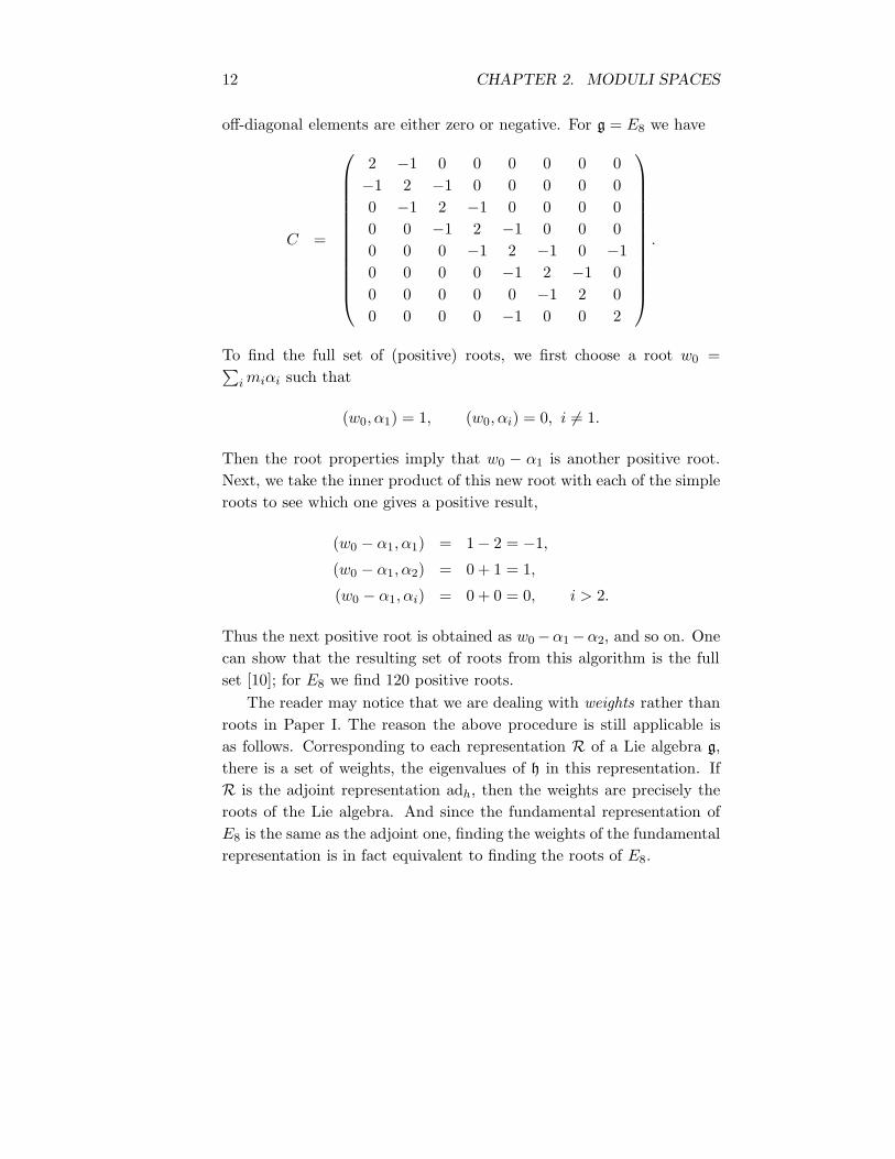
roots, we will demonstrate the procedure for that particular case here,but first we need to define another crucial ingredient in the Lie algebrasetup, the Cartan matrix. This is essentially a matrix of inner productsbetween simple roots. More precisely, the entries of the Cartan matrixC associated with the Lie algebra g are defined as
Cij ≡ 2(αi, αj)/(αj , αj),
where αi are the simple roots, i = 1, ..., rank(g), and ( · , · ) is the innerproduct on g. The diagonal elements are always equal to 2, while the
12 CHAPTER 2. MODULI SPACES
off-diagonal elements are either zero or negative. For g = E8 we have
C =
2 −1 0 0 0 0 0 0−1 2 −1 0 0 0 0 00 −1 2 −1 0 0 0 00 0 −1 2 −1 0 0 00 0 0 −1 2 −1 0 −10 0 0 0 −1 2 −1 00 0 0 0 0 −1 2 00 0 0 0 −1 0 0 2
.
To find the full set of (positive) roots, we first choose a root w0 =∑imiαi such that
(w0, α1) = 1, (w0, αi) = 0, i 6= 1.
Then the root properties imply that w0 − α1 is another positive root.Next, we take the inner product of this new root with each of the simpleroots to see which one gives a positive result,
(w0 − α1, α1) = 1− 2 = −1,
(w0 − α1, α2) = 0 + 1 = 1,
(w0 − α1, αi) = 0 + 0 = 0, i > 2.
Thus the next positive root is obtained as w0−α1−α2, and so on. Onecan show that the resulting set of roots from this algorithm is the fullset [10]; for E8 we find 120 positive roots.
The reader may notice that we are dealing with weights rather thanroots in Paper I. The reason the above procedure is still applicable isas follows. Corresponding to each representation R of a Lie algebra g,there is a set of weights, the eigenvalues of h in this representation. IfR is the adjoint representation adh, then the weights are precisely theroots of the Lie algebra. And since the fundamental representation ofE8 is the same as the adjoint one, finding the weights of the fundamentalrepresentation is in fact equivalent to finding the roots of E8.
2.3. N=2 SUPER-YANG-MILLS THEORY 13
2.2.3 Dynkin diagrams
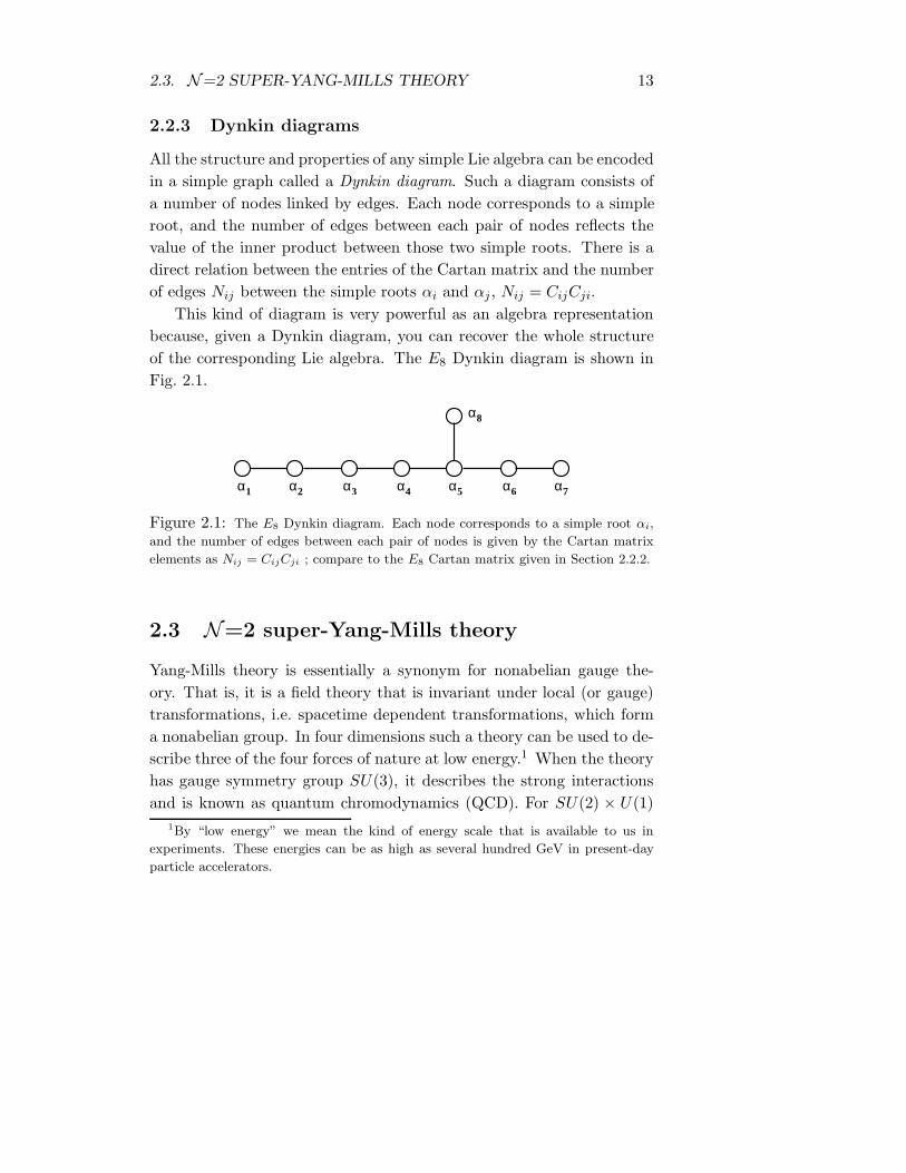
All the structure and properties of any simple Lie algebra can be encodedin a simple graph called a Dynkin diagram. Such a diagram consists ofa number of nodes linked by edges. Each node corresponds to a simpleroot, and the number of edges between each pair of nodes reflects thevalue of the inner product between those two simple roots. There is adirect relation between the entries of the Cartan matrix and the numberof edges Nij between the simple roots αi and αj , Nij = CijCji.
This kind of diagram is very powerful as an algebra representationbecause, given a Dynkin diagram, you can recover the whole structureof the corresponding Lie algebra. The E8 Dynkin diagram is shown inFig. 2.1.
α1 α2 α3 α4 α6 α7α5
α8
Figure 2.1: The E8 Dynkin diagram. Each node corresponds to a simple root αi,
and the number of edges between each pair of nodes is given by the Cartan matrix
elements as Nij = CijCji ; compare to the E8 Cartan matrix given in Section 2.2.2.
2.3 N=2 super-Yang-Mills theory
Yang-Mills theory is essentially a synonym for nonabelian gauge the-ory. That is, it is a field theory that is invariant under local (or gauge)transformations, i.e. spacetime dependent transformations, which forma nonabelian group. In four dimensions such a theory can be used to de-scribe three of the four forces of nature at low energy.1 When the theoryhas gauge symmetry group SU(3), it describes the strong interactionsand is known as quantum chromodynamics (QCD). For SU(2) × U(1)
1By “low energy” we mean the kind of energy scale that is available to us in
experiments. These energies can be as high as several hundred GeV in present-day
particle accelerators.
14 CHAPTER 2. MODULI SPACES
it unifies electromagnetic and weak interactions in the electroweak the-ory. Together, QCD and the electroweak theory constitute the StandardModel, which to date reproduces all known experimental results of par-ticle physics.
A gauge theory may possess other symmetries in addition to thegauge symmetry. For example there may be a global symmetry group;that is, the theory is invariant under some group of spacetime indepen-dent transformations. The intuitive physical picture of such a globalsymmetry is as a symmetry acting on added matter, for instance a num-ber of quarks in QCD.
Another symmetry example is supersymmetry, i.e. a symmetry be-tween bosons and fermions such that every boson is matched by afermion (a “superpartner”) with equal mass and charge. It may seemunmotivated to introduce such a symmetry, since in experiments we haveseen neither spin-0 particles with the mass of an electron, nor masslessspin-1
2 particles (“photinos”). But the idea is that the low-energy worldwe live in has spontaneously broken supersymmetry, while at sufficientlyhigh energy we would see the supersymmetry manifest. One promisingclue that this might be the case comes from the standard model couplingconstants. The theoretical prediction is that, without supersymmetry,they all are almost, but not quite, equal, at around 1014 GeV, whereasinclusion of supersymmetry makes them exactly identical, at an energyof around 1016 GeV.
If a nonabelian gauge theory is supersymmetric, it is called super-Yang-Mills (SYM) theory. Such a theory is also invariant under so-calledR-symmetry, which is essentially the symmetry group transforming thedifferent supersymmetry generators into each other.
We now define the precise type of SYM theories that interest us,before embarking on an analysis of their vacuum states.
2.3.1 Defining our SYM theory
There are several parameters we need to specify in order to define whichparticular type of SYM theory that we are interested in. First, SYMtheory can be defined in any dimension up to ten (see [5], Appendix B),
2.3. N=2 SUPER-YANG-MILLS THEORY 15
but the case relevant to us is the four-dimensional one (as the low-energyeffective action on a D3-brane).
We also need to specify the number of supersymmetries, N . Al-though the worldvolume theory in Paper I a priori has N=4 (see [5],Chapter 13), this supersymmetry is partially broken by putting thebranes on an orbifold singularity, and we end up with N=2. So wefocus here on N=2 SYM theory.
The next thing to specify is the field content.
Field content
A SYM theory contains a number of massless multiplets; the larger,massive multiplets can always be decomposed into these. The relevantmultiplet in “pure” N=2 SYM theory (i.e. there are only gauge fieldinteractions in the theory, and no matter added by hand) is a vectormultiplet containing gauge fields Aa
µ (a labels the gauge group genera-tors), two spinors λa
α and χaα, a complex scalar ϕa and a real auxiliary
field Da (see [5], Appendix B.2).All these fields transform in the adjoint representation of the gauge
group. This means that, under a transformation by an element g of thegauge group, a field φ transforms as
φ→ gφg−1.
On the other hand, it is said to transform in the fundamental represen-tation if it transforms as
φ→ gφ, φ† → φ†g−1,
where φ† is the Hermitian conjugate of φ. Finally, φ is said to transformin the antifundamental representation of G if it transforms as
φ→ φg−1, φ† → gφ†.
Sometimes the representations are denoted by fat numbers, so that afield transforming in the fundamental representation of, say, U(3), issaid to transform as 3 (3 is the dimension of this representation). The
16 CHAPTER 2. MODULI SPACES
antifundamental analogue is 3. Note that a field transforming in both 3and 3 of U(3) by definition transforms in the adjoint. Moreover, if a fieldtransforms under a product of groups, say U(2) × U(3), as (2, 3), thenwe call it a bifundamental field. This notation will be relevant when wediscuss quiver gauge theories in Section 2.5.
We now add some fundamental matter to our pureN=2 SYM theory.More precisely, we introduce two hypermultiplets, each of which consistsof a complex scalar field φi (i = 1, 2 labels the two hypermultiplets), aspinor ψi and a complex auxiliary field2 F i, and they all transform inthe fundamental representation of the gauge group.
2.3.2 Spontaneous symmetry breaking
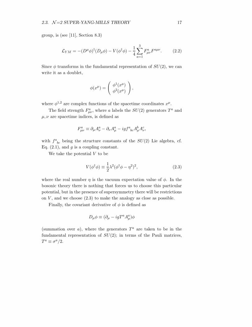
Due to the shape of the potential in N=2 SYM theory, the gauge sym-metry may be spontaneously broken. This happens because, instead ofa unique vacuum with zero energy, there is a whole family of vacua.Rather than being individually invariant under gauge symmetry trans-formations, these vacua are transformed into each other. The physicalsystem will spontaneously choose one of the vacua, thus breaking thegauge symmetry. This process goes by the name Higgs mechanism, aphysical example of which is superconductivity (see e.g. [11], Chapter 8).The gauge-broken theory describes the dynamics of the chosen vacuumfield, which parameterises the moduli space, i.e. the space of vacua, ofthe theory.
To illustrate the principle of the Higgs mechanism, we now considerthe bosonic Yang-Mills theory with SU(2) gauge symmetry.
SU(2) bosonic Yang-Mills
We first write down the Lagrangian and then define the constituentfields. The Yang-Mills Lagrangian, with one matter (complex scalar)field φ transforming in the fundamental representation of the gauge
2F i is called an auxiliary field because it has no kinetic energy term. That is, its
equations of motion are purely algebraic and it can be expressed in terms of other
dynamical fields.
2.3. N=2 SUPER-YANG-MILLS THEORY 17
group, is (see [11], Section 8.3)
LY M = −(Dµφ)†(Dµφ)− V (φ†φ)− 14
3∑a=1
F aµνF
aµν . (2.2)
Since φ transforms in the fundamental representation of SU(2), we canwrite it as a doublet,
φ(xµ) =
(φ1(xµ)φ2(xµ)
),
where φ1,2 are complex functions of the spacetime coordinates xµ.The field strength F a
µν , where a labels the SU(2) generators T a andµ, ν are spacetime indices, is defined as
F aµν ≡ ∂µA
aν − ∂νA
aµ − igfa
bcAbµA
cν ,
with fabc being the structure constants of the SU(2) Lie algebra, cf.
Eq. (2.1), and g is a coupling constant.We take the potential V to be
V (φ†φ) ≡ 12λ2(φ†φ− η2)2, (2.3)
where the real number η is the vacuum expectation value of φ. In thebosonic theory there is nothing that forces us to choose this particularpotential, but in the presence of supersymmetry there will be restrictionson V , and we choose (2.3) to make the analogy as close as possible.
Finally, the covariant derivative of φ is defined as
Dµφ ≡ (∂µ − igT aAaµ)φ
(summation over a), where the generators T a are taken to be in thefundamental representation of SU(2); in terms of the Pauli matrices,T a ≡ σa/2.
18 CHAPTER 2. MODULI SPACES
The Higgs mechanism
We are interested in the classical vacua of this theory. These are definedby the vanishing of the potential (2.3), so any vacuum φ0 must satisfyφ†0φ0 = η2. As mentioned above, the φ0’s are not themselves gaugeinvariant, but V is, and there is a continuous family of vacua φ0related by SU(2) transformations. These vacua parameterise what iscalled a “flat” direction.
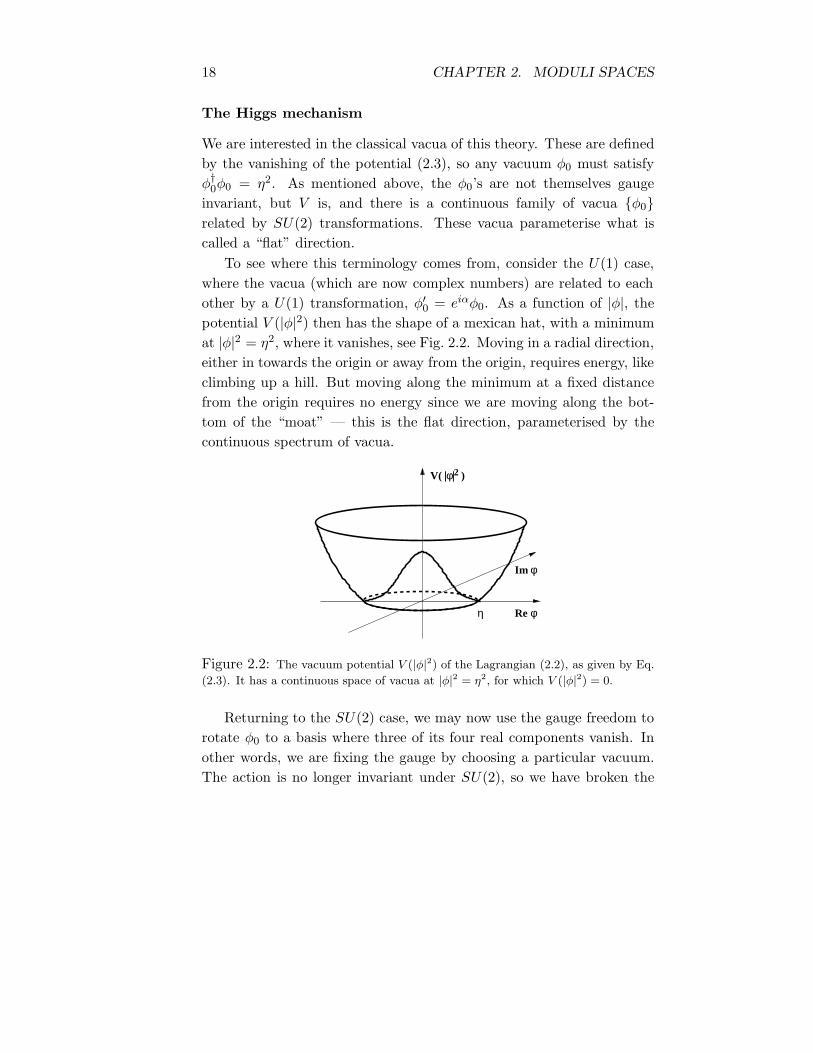
To see where this terminology comes from, consider the U(1) case,where the vacua (which are now complex numbers) are related to eachother by a U(1) transformation, φ′0 = eiαφ0. As a function of |φ|, thepotential V (|φ|2) then has the shape of a mexican hat, with a minimumat |φ|2 = η2, where it vanishes, see Fig. 2.2. Moving in a radial direction,either in towards the origin or away from the origin, requires energy, likeclimbing up a hill. But moving along the minimum at a fixed distancefrom the origin requires no energy since we are moving along the bot-tom of the “moat” — this is the flat direction, parameterised by thecontinuous spectrum of vacua.
Re φ
Im φ
η
2|φ|V( )
Figure 2.2: The vacuum potential V (|φ|2) of the Lagrangian (2.2), as given by Eq.
(2.3). It has a continuous space of vacua at |φ|2 = η2, for which V (|φ|2) = 0.
Returning to the SU(2) case, we may now use the gauge freedom torotate φ0 to a basis where three of its four real components vanish. Inother words, we are fixing the gauge by choosing a particular vacuum.The action is no longer invariant under SU(2), so we have broken the

2.3. N=2 SUPER-YANG-MILLS THEORY 19
gauge symmetry; we have spontaneous symmetry breaking. However,note that the gauge symmetry is not completely broken. The Lagrangian(2.2) is still invariant under U(1) transformations, so the gauge grouphas been broken from SU(2) down to a U(1) subgroup.
We are thus left with one real component in φ0, which we write as asum of a constant part η and a nonconstant part γ(xµ),
φ0 =
(0
η + γ(xµ)
). (2.4)
If one inserts (2.4) into the Lagrangian (2.2) and expands the latter, onefinds that it contains mass terms for the gauge bosons [12]. That is,there are quadratic terms of the form m2
AAaµA
aµ, where the mass mA isproportional to the parameter η.
In conclusion, spontaneous breaking of the gauge symmetry rendersthe gauge bosons massive; in the SU(2) × U(1) case they combine intothe W- and Z-bosons (see [11], Section 8.5). The field φ0 in this contextis called a Higgs field, and its vacuum expectation value η is the Higgsmass.
2.3.3 The N=2 potential
The Higgs mechanism generalises straightforwardly to the supersymmet-ric theory. The difference is that supersymmetry imposes constraints onthe form of the action. For instance, the potential cannot be arbitrary,and in addition the number of scalar fields is restricted.
The action for N=2 SYM theory is much more complicated thanthe bosonic one, as it involves all the fields in the vector multiplet (ϕa,χa
α, λaβ, Aa
µ, Da) plus any hypermultiplets (φi, ψi, F i) added by hand, aswell as their interactions. In superspace formalism (see Section 3.3 fordetails) this action looks simpler, but we omit it here since we do notneed to work with it explicitly. For a pedagogical account of the N=2SU(2) SYM action, see e.g. [13]. Here it suffices to say that to find thepotential for the scalar matter fields (which we need for deriving themoduli space), one expands the action in components and extracts all
20 CHAPTER 2. MODULI SPACES
terms containing the auxiliary fields Da and F i. This yields a sum ofD-terms and F-terms, and then we integrate out Da and F i by use oftheir equations of motion. The result is a potential involving a sum ofcommutators between all scalar fields3 ϕa and φi.
Fayet-Iliopoulos terms
However, this is not the whole story. In a supersymmetric gauge theory,the precise form of the potential depends on the number of U(1) factorspresent in the gauge group. This is because supersymmetry allows anextra term in the action when the gauge group contains a U(1) factor (see[5], Appendix B). This extra term is of the form ξkDk, with Dk being thek:th U(1)-component of Da, and ξk is a real parameter, called the Fayet-Iliopoulos term (FI-term). Thus the FI-parameter corresponding to thegenerator T a is ξa with a running over all the gauge group generators,but with ξa 6= 0 only for a = k, where k labels the U(1) generators.
In N=1 SYM there is only one, real FI-term for each U(1) fac-tor. N=2 supersymmetry, on the other hand, allows three differentFI-parameters for each U(1); this is due to the SU(2) R-symmetry thatrelates the two supersymmetries. The three FI-terms transform as atriplet under the SU(2) R-symmetry [14], and we denote them as athree-vector ~ξa.
The potential
Let us finally have a look at the potential for the scalar fields in ourSYM theory:
V = Tr([ϕ,ϕ†]2) +∑i=1,2
φi[ϕ,ϕ†]φi +dim G∑a=1
(Tr [T a · ~µ]− ~ξa
)2, (2.5)
where a barred index implies Hermitian conjugate, φi ≡ φi †. The three-vector ~µ is defined as
~µ ≡ Tr(φ†~σφ
), (2.6)
3Note that each scalar field is usually represented by a matrix, so the commutators
become matrix commutators.
2.3. N=2 SUPER-YANG-MILLS THEORY 21
where φ is the quaternion of the φi’s,
φ =
(φ1 † φ2 †
−φ2 φ1
), (2.7)
and ~σ = (σ1, σ2, σ3) are the Pauli matrices.Note that each of the φi’s is a matrix of rank equal to that of G.
Similarly ~µ is a three-vector of matrices of rank equal to rank(G); thetrace in (2.6) is in the 2×2 basis of the Pauli matrices, not over thematrices φi. On the other hand, the trace in the last term in Eq. (2.5)is in the rank(G) basis, and its effect is to project ~µ explicitly onto thebasis vectors T a.
We now use the potential (2.5) to find the vacuum moduli space.
2.3.4 The SYM moduli space
To find the vacua we set V = 0 and solve for the scalars. In a wayanalogous to the bosonic analysis, we may fix the gauge and give nonzeroexpectation values to the scalars. We thus end up with a low-energyeffective theory with a gauge symmetry that is a subgroup of the originalgauge group G, and massless scalars constituting the moduli space.
Note that although nonzero expectation values of the scalars breakthe gauge symmetry, they leave the supersymmetry unbroken. This isbecause any vacuum state with zero energy (which is by definition truefor the Higgs fields) is supersymmetric as a direct consequence of thesupersymmetry algebra [15]. So in the case at hand, the gauge-fixedtheory also is N=2 invariant, just like its G-symmetric parent.
What is the geometry of the moduli space? There are a few differentpossibilities, depending on the FI-terms. We first study the case whereall the FI-terms vanish; it is then clear from (2.5) that the potentialcannot vanish when both ϕa and φi take generic values. So we havetwo possibilities: ϕa 6= 0 and φi = 0 on the one hand, and on the otherhand ϕa = 0 and φi 6= 0. Thus the moduli space consists of two distinctspaces, or branches.
In the first case, when all hypermultiplets are zero, we find a familyof vacua ϕ0 that transform into each other under G. Spontaneous
22 CHAPTER 2. MODULI SPACES
symmetry breaking renders all but one gauge boson massive and we areleft with one massless scalar ϕ0. The moduli space is then complex-one-dimensional, parameterised by the gauge invariant quantity u ≡〈Tr(ϕ0)2〉. This space, induced by the vector multiplet, is called theCoulomb branch. It is required by N=2 supersymmetry to be a rigidspecial Kahler manifold [16]; in a four-dimensional theory it is P
1.Keeping ϕa = 0 on the other hand, and giving expectation val-
ues to φi defines another branch of the moduli space, called the Higgsbranch, and N=2 supersymmetry requires it to be a hyperkahler man-ifold [17]. This is a real-4k-dimensional (k an integer) manifold withSp(k) holonomy.4 It comes equipped with three complex structures andthree moment maps.
Actually, the Higgs branch in this particular case has singularities;it is an orbifold with fixed points. Thus it is not a manifold in the strictsense; however, it is the singular limit of a hyperkahler manifold, and assuch it possesses all the structure of a smooth hyperkahler manifold. Anexample is the K3 orbifold, i.e. the orbifold limit of a compact complex-two-dimensional hyperkahler manifold with SU(2) holonomy. Or rather,we will be interested in orbifolds of the form C
2/Γ (where Γ is a discretesubgroup of SU(2)), which may be viewed as a local description of a K3orbifold near one of its singularities.
2.3.5 Singularities
The appearance of singularities on the moduli space is due to the waywe discard massive fields in the low-energy effective theory of the Higgsfields. One can show that, if the gauge-fixed scalars (the Higgs fields) areinserted into the SYM action, most of the gauge fields acquire massesproportional to the vacuum expectation values of the Higgs fields [13], inanalogy with the bosonic case. These gauge fields may then be neglectedin the low-energy effective theory describing the gauge-fixed (massless)scalars; we say that the gauge bosons have been “higgsed away.”
4The holonomy of a manifold is the subgroup of O(n) under which a vector trans-
forms as it is parallel-transported around a closed loop on an n-dimensional manifold.
2.3. N=2 SUPER-YANG-MILLS THEORY 23
The fact that the gauge-fixed theory includes only the massless fieldsin the bulk (away from the origin of the moduli space) means that themoduli space contains a singularity at the origin. The reason is that, asthe Higgs masses (the vacuum expectation values) approach zero, theformerly massive fields become massless, and thus become relevant inthe theory. Therefore the low-energy effective bulk theory cannot beaccurate near the origin.
This is true classically for both branches; there is a singularity at theorigin of the Higgs branch which coincides with the singularity at theorigin of the Coulomb branch. However, when we pass to the quantumlevel, the singularity of the Coulomb branch splits into several separatesingularities depending on the gauge group [18]. The physical interpre-tation of the quantum singularities is not as straightforward as in theclassical case (gauge bosons becoming massless), but for SU(2) SYM itwas shown in [19] that two singularities arise on the Coulomb branch,and that they correspond to a pair of dyons (bound states of electric andmagnetic charges) becoming massless (see also [13]). Due to N=2 super-symmetry, the Higgs branch receives no quantum corrections [19, 20].
2.3.6 Nonzero FI-terms
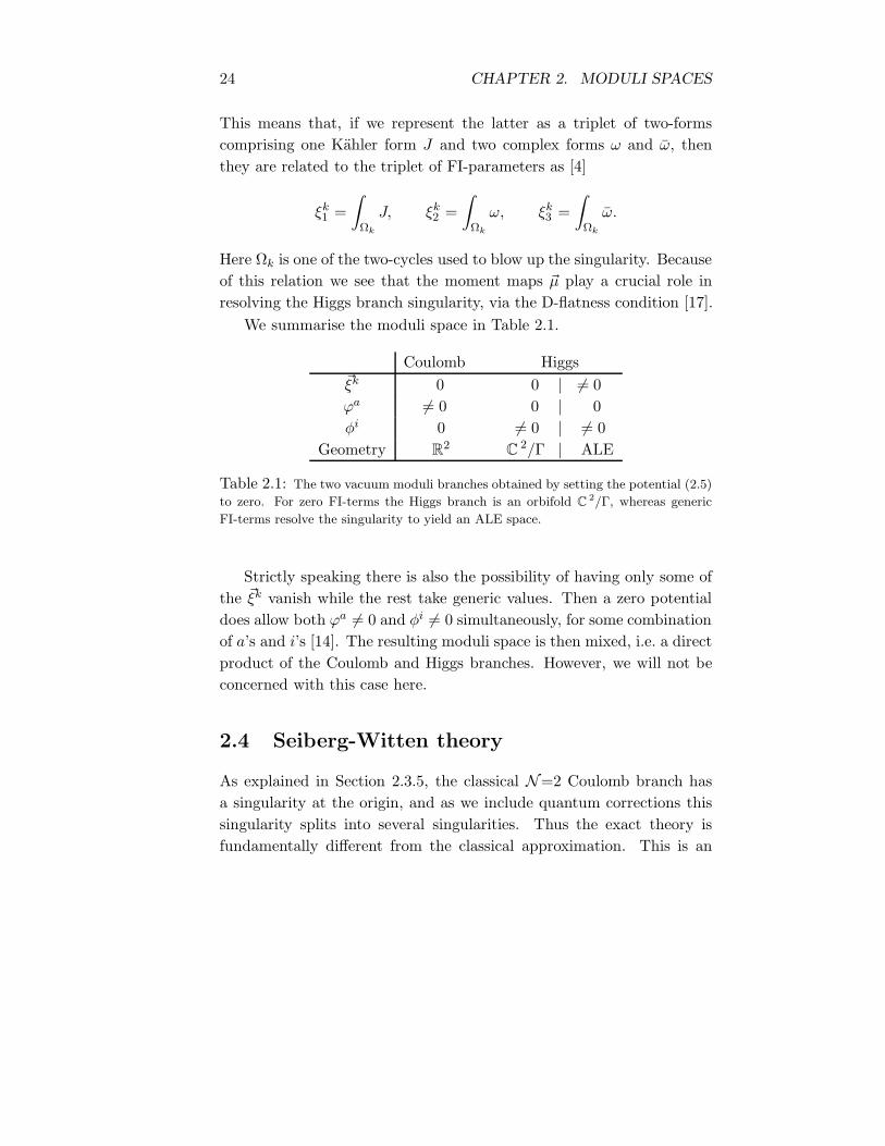
Continuing our investigation of the vacuum moduli space, it remains tosee what happens when all of the FI-terms ~ξk are nonzero and generic.In this case the full potential (2.5) can vanish only if all the vectormultiplets ϕa are zero, which leaves only the last term, involving themoment map. The vanishing of this term is commonly referred to as theD-flatness condition. Since ϕa = 0, we again get a Higgs branch, exceptthis time it looks a little bit different. It is again an orbifold, but withits singularity resolved, or “blown up.” In geometric terms, this blow-upis done essentially by replacing the singularity with a connected unionof intersecting two-spheres (two-cycles), and the FI-terms parameterisethe size of these spheres [4]. The resulting smooth space is then a truehyperkahler manifold, called an asymptotically locally Euclidean (ALE)space.
The FI-terms are in fact the periods of the hyperkahler structures.
24 CHAPTER 2. MODULI SPACES
This means that, if we represent the latter as a triplet of two-formscomprising one Kahler form J and two complex forms ω and ω, thenthey are related to the triplet of FI-parameters as [4]
ξk1 =
∫Ωk
J, ξk2 =
∫Ωk
ω, ξk3 =
∫Ωk
ω.
Here Ωk is one of the two-cycles used to blow up the singularity. Becauseof this relation we see that the moment maps ~µ play a crucial role inresolving the Higgs branch singularity, via the D-flatness condition [17].
We summarise the moduli space in Table 2.1.
Coulomb Higgs~ξk 0 0 | 6= 0ϕa 6= 0 0 | 0φi 0 6= 0 | 6= 0
Geometry R2
C2/Γ | ALE
Table 2.1: The two vacuum moduli branches obtained by setting the potential (2.5)
to zero. For zero FI-terms the Higgs branch is an orbifold C2/Γ, whereas generic
FI-terms resolve the singularity to yield an ALE space.
Strictly speaking there is also the possibility of having only some ofthe ~ξk vanish while the rest take generic values. Then a zero potentialdoes allow both ϕa 6= 0 and φi 6= 0 simultaneously, for some combinationof a’s and i’s [14]. The resulting moduli space is then mixed, i.e. a directproduct of the Coulomb and Higgs branches. However, we will not beconcerned with this case here.
2.4 Seiberg-Witten theory
As explained in Section 2.3.5, the classical N=2 Coulomb branch hasa singularity at the origin, and as we include quantum corrections thissingularity splits into several singularities. Thus the exact theory isfundamentally different from the classical approximation. This is an
2.4. SEIBERG-WITTEN THEORY 25
indication of the fact that perturbation theory cannot be used in theregion near the origin since the theory is strongly coupled there.
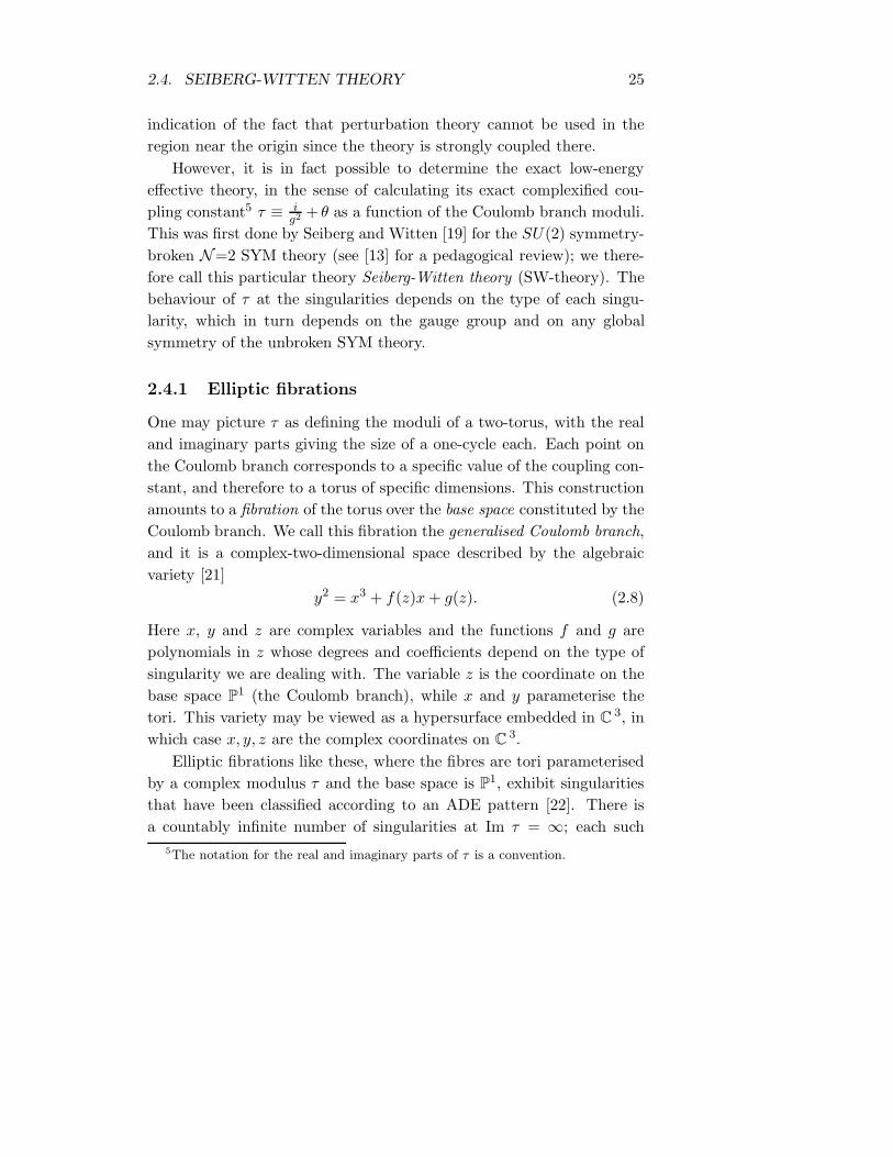
However, it is in fact possible to determine the exact low-energyeffective theory, in the sense of calculating its exact complexified cou-pling constant5 τ ≡ i
g2 + θ as a function of the Coulomb branch moduli.This was first done by Seiberg and Witten [19] for the SU(2) symmetry-broken N=2 SYM theory (see [13] for a pedagogical review); we there-fore call this particular theory Seiberg-Witten theory (SW-theory). Thebehaviour of τ at the singularities depends on the type of each singu-larity, which in turn depends on the gauge group and on any globalsymmetry of the unbroken SYM theory.
2.4.1 Elliptic fibrations
One may picture τ as defining the moduli of a two-torus, with the realand imaginary parts giving the size of a one-cycle each. Each point onthe Coulomb branch corresponds to a specific value of the coupling con-stant, and therefore to a torus of specific dimensions. This constructionamounts to a fibration of the torus over the base space constituted by theCoulomb branch. We call this fibration the generalised Coulomb branch,and it is a complex-two-dimensional space described by the algebraicvariety [21]
y2 = x3 + f(z)x+ g(z). (2.8)
Here x, y and z are complex variables and the functions f and g arepolynomials in z whose degrees and coefficients depend on the type ofsingularity we are dealing with. The variable z is the coordinate on thebase space P
1 (the Coulomb branch), while x and y parameterise thetori. This variety may be viewed as a hypersurface embedded in C
3, inwhich case x, y, z are the complex coordinates on C
3.Elliptic fibrations like these, where the fibres are tori parameterised
by a complex modulus τ and the base space is P1, exhibit singularities
that have been classified according to an ADE pattern [22]. There isa countably infinite number of singularities at Im τ = ∞; each such
5The notation for the real and imaginary parts of τ is a convention.

26 CHAPTER 2. MODULI SPACES
singularity is of type either An or Dn, for integer n. In addition thereare seven singularities at finite values of τ , of types A0, A1, A2, D4, E6,E7 and E8, respectively.
When z approaches one of the singularities on the Coulomb branchthe torus fibre degenerates in a specific way depending on the singularitytype. For instance, if the singularity is of type An, the torus is “pinched”in n + 1 places so that it becomes a necklace of two-spheres joined atpoints, as illustrated in Fig. 2.3. This singular hypersurface is thendescribed by (2.8) for some specific polynomials f and g; for A2, forinstance, f goes to zero and g = z2, so that the algebraic variety becomesy2 = x3 + z2.
Figure 2.3: The toroidal fibre at an A4 singularity. The torus is “pinched” in five
places so that it becomes a necklace of five two-spheres joined at points.
2.4.2 Connection to physics
This ADE classification of the fibration (2.8) is a purely mathematicalresult, but due to the interpretation of the torus modulus τ as a couplingconstant, it has inspired a line of physics investigations that has provedvery fruitful. The idea is that each of the singularities listed above cor-responds to a four-dimensional N=2 SYM theory with global symmetrycorresponding to the singularity type. In particular, the interesting the-ories are the ones at strong coupling, i.e. at the seven singularities atfinite τ (Im τ = ∞ corresponds to weak coupling).
For instance, the original Seiberg-Witten theory, i.e. N=2 SYM withSU(2) gauge group and four hypermultiplets (which has SO(8,C ) global

2.4. SEIBERG-WITTEN THEORY 27
symmetry), fits nicely in this picture as the strongly coupled theory atthe D4 singularity. The A0, A1 and A2 theories (i.e. they have globalsymmetries SL(1,C ), SL(2,C ) and SL(3,C )) are obtained as certainlimits of an SU(2) gauge theory with respectively one, two and threehypermultiplets [23, 24]; these theories can be derived from the D4 the-ory.
The success of this correspondence thus far then prompted the corre-sponding computation for the E6, E7 and E8 theories, i.e. theories withexceptional global symmetries6 [25, 26, 27]. The existence of such SW-theories7 has been shown also via compactifications of higher-dimensionalgauge theories [28]. The computation of exceptional varieties is ex-plained in detail in e.g. [29].
2.4.3 Brane picture
The picture of the coupling constant as a torus parameter has given riseto the idea of F-theory [30]. This is a conjectured twelve-dimensionaltheory which, when compactified on a four-dimensional K3 manifold, isequivalent to Type IIB theory compactified on a two-dimensional man-ifold such as a sphere or a two-torus. The K3 manifold is a fibrationof tori over the two-dimensional manifold, and the coupling constant τparameterises the fibre tori.
To see how this picture is relevant to us, we need to go into somedetail. Take the two-dimensional base space to be P
1, parameterisedby the complex coordinate z. Then the K3 manifold is described byan algebraic variety of the form (2.8) with f and g being of degreeeight and twelve respectively in z, and it has 24 singularities. Theseare determined as the zeroes of the discriminant of the variety [21], andcorrespond in the IIB picture to the positions on P
1 of 24 spacefilling7-branes (filling up the eight uncompactified dimensions) [31].
6As Lagrangian descriptions do not exist for the exceptional theories, the authors
of [25, 26, 27] had to resort to more indirect methods of determining the generalised
Coulomb branch.7We extend the name SW-theory to include all the aforementioned strongly cou-
pled ADE theories.
28 CHAPTER 2. MODULI SPACES
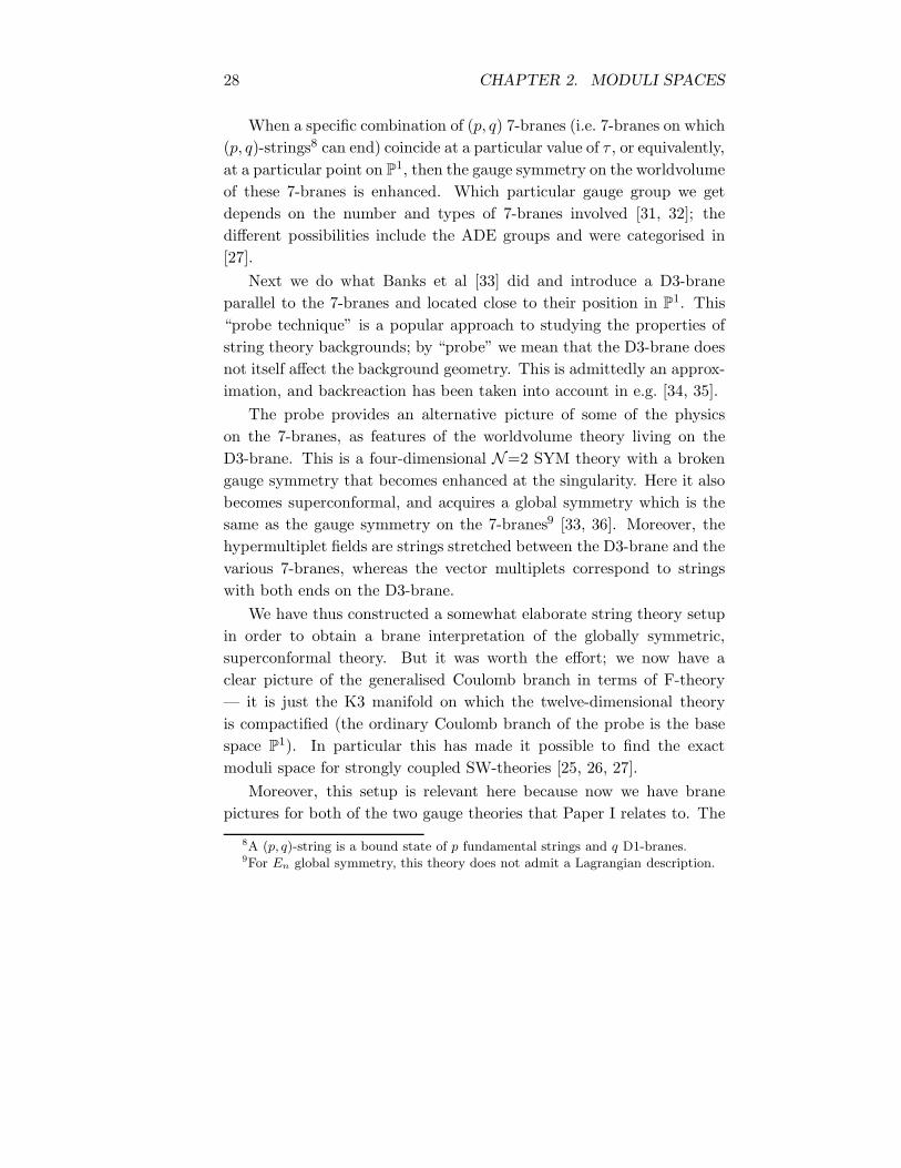
When a specific combination of (p, q) 7-branes (i.e. 7-branes on which(p, q)-strings8 can end) coincide at a particular value of τ , or equivalently,at a particular point on P
1, then the gauge symmetry on the worldvolumeof these 7-branes is enhanced. Which particular gauge group we getdepends on the number and types of 7-branes involved [31, 32]; thedifferent possibilities include the ADE groups and were categorised in[27].
Next we do what Banks et al [33] did and introduce a D3-braneparallel to the 7-branes and located close to their position in P
1. This“probe technique” is a popular approach to studying the properties ofstring theory backgrounds; by “probe” we mean that the D3-brane doesnot itself affect the background geometry. This is admittedly an approx-imation, and backreaction has been taken into account in e.g. [34, 35].
The probe provides an alternative picture of some of the physicson the 7-branes, as features of the worldvolume theory living on theD3-brane. This is a four-dimensional N=2 SYM theory with a brokengauge symmetry that becomes enhanced at the singularity. Here it alsobecomes superconformal, and acquires a global symmetry which is thesame as the gauge symmetry on the 7-branes9 [33, 36]. Moreover, thehypermultiplet fields are strings stretched between the D3-brane and thevarious 7-branes, whereas the vector multiplets correspond to stringswith both ends on the D3-brane.
We have thus constructed a somewhat elaborate string theory setupin order to obtain a brane interpretation of the globally symmetric,superconformal theory. But it was worth the effort; we now have aclear picture of the generalised Coulomb branch in terms of F-theory— it is just the K3 manifold on which the twelve-dimensional theoryis compactified (the ordinary Coulomb branch of the probe is the basespace P
1). In particular this has made it possible to find the exactmoduli space for strongly coupled SW-theories [25, 26, 27].
Moreover, this setup is relevant here because now we have branepictures for both of the two gauge theories that Paper I relates to. The
8A (p, q)-string is a bound state of p fundamental strings and q D1-branes.9For En global symmetry, this theory does not admit a Lagrangian description.
2.5. QUIVER GAUGE THEORY 29
other theory, the quiver gauge theory, which has a more straightforwardbrane interpretation, is discussed in the next section. But first we remarkthat since, as was shown in [8, 9] and Paper I, there is a nontrivialidentity between the moduli spaces of these two different theories, weexpect there to be some kind of duality between the two string theorybackgrounds. However, this turns out to be less than manifest, andattempts at finding such a duality have failed thus far (see e.g. [37]).
Let us now explain what we mean by a quiver theory.
2.5 Quiver gauge theory
Quiver gauge theory is a well-established concept that frequently cropsup in string theory [14, 38]. At first sight this type of theory may seemanything but natural, as it involves a rather specific gauge structure —a product of unitary groups and matter fields transforming according toa strict pattern as bifundamentals under pairs of the constituent gaugegroups. However, in the quest for realistic physics based on string theoryone must break both supersymmetry and gauge symmetry in some way,and one of the most straightforward procedures yields precisely what wecall quiver theory.
The idea is to start with Type IIB string theory in ten flat dimen-sions (coordinates x0, x1, ..., x9) and introduce a stack of N coincidingD3-branes. We arrange these branes such that their four-dimensionalworldvolumes are aligned with the 0-1-2-3-directions x0, ..., x3. Theworldvolume supports a pure N=4 SYM theory, i.e. the only matterpresent is a vector multiplet containing three complex (= six real) scalarfields transforming in the adjoint representation of the gauge group. Inthe string theory picture these scalars are the coordinates of the positionof the branes along the six dimensions transverse to the branes. As longas they all coincide, the gauge symmetry is U(N); this is due to the wayin which the ends of open strings are indexed (by Chan-Paton indices)according to which branes in the stack they are attached to (see [39],Section 6.5).
However, if the branes separate from each other, the gauge group
30 CHAPTER 2. MODULI SPACES
is broken down to some subgroup, since there will be fewer branes formassless strings to end on. This is precisely the Higgs mechanism fromthe point of view of the gauge theory; moving the branes correspondsto giving expectation values to the scalar fields, which breaks the gaugesymmetry.
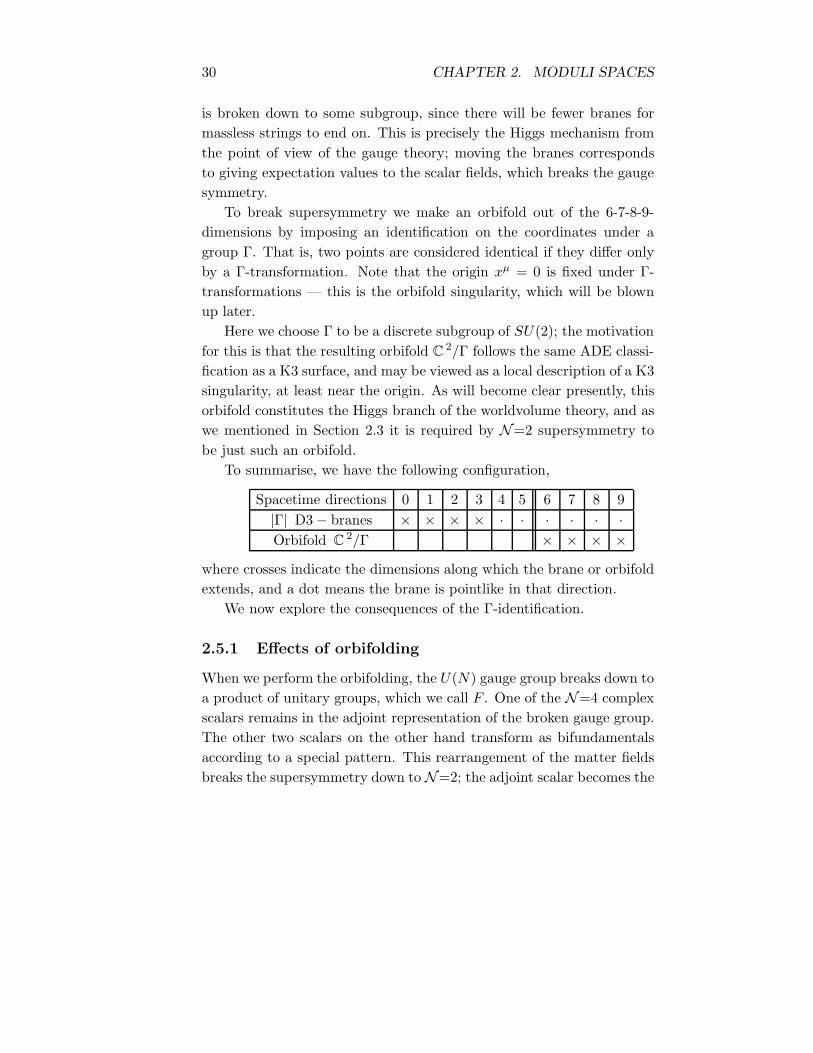
To break supersymmetry we make an orbifold out of the 6-7-8-9-dimensions by imposing an identification on the coordinates under agroup Γ. That is, two points are considered identical if they differ onlyby a Γ-transformation. Note that the origin xµ = 0 is fixed under Γ-transformations — this is the orbifold singularity, which will be blownup later.
Here we choose Γ to be a discrete subgroup of SU(2); the motivationfor this is that the resulting orbifold C
2/Γ follows the same ADE classi-fication as a K3 surface, and may be viewed as a local description of a K3singularity, at least near the origin. As will become clear presently, thisorbifold constitutes the Higgs branch of the worldvolume theory, and aswe mentioned in Section 2.3 it is required by N=2 supersymmetry tobe just such an orbifold.
To summarise, we have the following configuration,
Spacetime directions 0 1 2 3 4 5 6 7 8 9|Γ| D3− branes × × × × · · · · · ·Orbifold C
2/Γ × × × ×
where crosses indicate the dimensions along which the brane or orbifoldextends, and a dot means the brane is pointlike in that direction.
We now explore the consequences of the Γ-identification.
2.5.1 Effects of orbifolding
When we perform the orbifolding, the U(N) gauge group breaks down toa product of unitary groups, which we call F . One of the N=4 complexscalars remains in the adjoint representation of the broken gauge group.The other two scalars on the other hand transform as bifundamentalsaccording to a special pattern. This rearrangement of the matter fieldsbreaks the supersymmetry down to N=2; the adjoint scalar becomes the
2.5. QUIVER GAUGE THEORY 31
scalar in the N=2 vector multiplet, while the two bifundamentals con-stitute the scalars of two hypermultiplets. Thus the worldvolume theoryon the branes is now an N=2 SYM theory with two hypermultiplets.
It is easy to see explicitly how the orbifolding acts on the gaugegroup and the scalars. A detailed account of the orbifolding procedureis given in [14], and we merely sketch it here. The fields that we areinterested in, namely the vector fields Aa
µ (a labels the gauge groupgenerators), the complex 4-5-coordinate ϕ ≡ x4 + ix5, and the complex6-7-8-9-coordinates φ1 ≡ x6 + ix7 and φ2 ≡ x8 + ix9, all arise as masslessexcitations of open strings. We can therefore represent them by matri-ces encoding their Chan-Paton indices. With N branes present, thesematrices have dimension N ×N with, in a suitable basis, the (i,j) entryspecifying whether or not the string stretches between the i:th and j:thbranes.
Here we take the number of branes to equal the order of the orbifoldgroup, N = |Γ|. Although the reason for this choice will become clearlater, we attempt to justify it already at this point. Our aim is torepresent the action of Γ on the open string sector, and since there are|Γ| distinct elements of the orbifold group, we need |Γ| different stringstates to represent them. Therefore the strings need to be able to end on|Γ| different branes; these string states provide a faithful representationof Γ.
We use the following notation for the Chan-Paton matrices,
Aaµ → λa
V , (2.9)
ϕ → λI , (2.10)
φ1 → λ1II , (2.11)
φ2 → λ2II . (2.12)
In the unorbifolded theory, all these fields belong to the vector multipletand therefore transform in the adjoint representation of the unbrokengauge group U(|Γ|). However, the requirement that they be invariantunder the orbifold group Γ imposes restrictions on the Chan-Paton ma-trices such that this is no longer true.
32 CHAPTER 2. MODULI SPACES
If we denote by γΓ the regular matrix representation10 of Γ, then afield is Γ-invariant if it commutes with γΓ. We therefore impose
λaV = γΓλ
aV γ
−1Γ , (2.13)
λI = γΓλIγ−1Γ . (2.14)
For φ1,2, however, we need to take into account the fact that they livealong the orbifold directions. This means that the invariance conditioninvolves an extra Γ-action on the doublet (φ1, φ2), via the 2×2 matrixrepresentation acting on the quaternion11 (2.7). We call this matrix GΓ,and find the following invariance condition for φi,
λiII = (GΓ)ij γΓλ
jIIγ
−1Γ . (2.15)
It is now a matter of straightforward matrix algebra to derive the form ofthe Chan-Paton matrices that satisfy Eqs. (2.13)–(2.15), and the resultis the aforementioned factorisation of the gauge group and the bifun-damental structure. Some explicit such calculations are shown in e.g.[37].
Note that the vacuum moduli space now consists of two branches,as expected of a four-dimensional N=2 theory. The 4-5-space, inducedby the vector multiplet ϕ, constitutes the Coulomb branch, and theorbifolded 6-7-8-9-space, induced by the hypermultiplets φi, is the Higgsbranch.
So what about the Fayet-Iliopoulos terms? To find the correspondingobject in the string theory picture it is not sufficient to look only atthe open string sector. We need to include massless closed strings, inparticular the twisted ones. That is, string states that are invariantunder the orbifold group only as long as they stay at the singularity.These states enter the worldvolume theory of the D3-branes in exactlythe same way as FI-terms [14].
10The regular representation of a group G is the representation corresponding to
the left action of G on itself. In matrix form it is a |G|×|G| block-diagonal matrix
with each k-dimensional irreducible representation occurring k times on the diagonal.11For explicit matrix representations of the ADE groups, see e.g. [14, 37].
2.5. QUIVER GAUGE THEORY 33
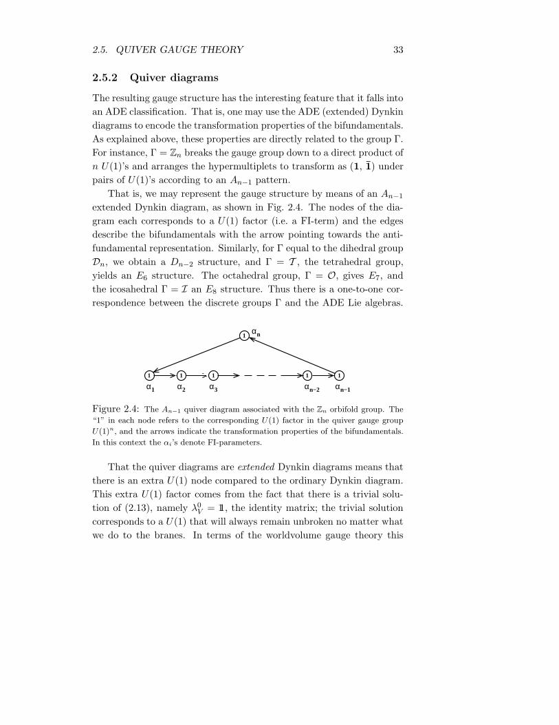
2.5.2 Quiver diagrams
The resulting gauge structure has the interesting feature that it falls intoan ADE classification. That is, one may use the ADE (extended) Dynkindiagrams to encode the transformation properties of the bifundamentals.As explained above, these properties are directly related to the group Γ.For instance, Γ = Zn breaks the gauge group down to a direct product ofn U(1)’s and arranges the hypermultiplets to transform as (1, 1) underpairs of U(1)’s according to an An−1 pattern.
That is, we may represent the gauge structure by means of an An−1
extended Dynkin diagram, as shown in Fig. 2.4. The nodes of the dia-gram each corresponds to a U(1) factor (i.e. a FI-term) and the edgesdescribe the bifundamentals with the arrow pointing towards the anti-fundamental representation. Similarly, for Γ equal to the dihedral groupDn, we obtain a Dn−2 structure, and Γ = T , the tetrahedral group,yields an E6 structure. The octahedral group, Γ = O, gives E7, andthe icosahedral Γ = I an E8 structure. Thus there is a one-to-one cor-respondence between the discrete groups Γ and the ADE Lie algebras.
α1 α2 α3
1 1 1 1 1
1
α α
αn
n−2 n−1
Figure 2.4: The An−1 quiver diagram associated with the Zn orbifold group. The
“1” in each node refers to the corresponding U(1) factor in the quiver gauge group
U(1)n, and the arrows indicate the transformation properties of the bifundamentals.
In this context the αi’s denote FI-parameters.
That the quiver diagrams are extended Dynkin diagrams means thatthere is an extra U(1) node compared to the ordinary Dynkin diagram.This extra U(1) factor comes from the fact that there is a trivial solu-tion of (2.13), namely λ0
V = 11, the identity matrix; the trivial solutioncorresponds to a U(1) that will always remain unbroken no matter whatwe do to the branes. In terms of the worldvolume gauge theory this
34 CHAPTER 2. MODULI SPACES
means we can Higgs away all the vector multiplets except the one corre-sponding to the trivial U(1). This U(1) group is the gauge group in theworldvolume theory of a single D-brane, so we see that the hypermulti-plets now parameterise the position in the orbifold of a single D3-brane.From the point of view of the covering space C
2, this brane is actuallya stack of |Γ| fractional branes, moving simultaneously in such a waythat they are images of each other under Γ.
2.6 The N=2 Higgs branch
The object of Paper I was to show that the Higgs branch of the E8 quivertheory is identical to the generalised Coulomb branch of E8 Seiberg-Witten theory. There is no problem to do this in the singular limit; thenthe quiver Higgs branch is just the orbifold C
2/I, which is describedessentially by Eq. (2.8) with f(z) = 0 and g(z) = z5.
The subtle difference is that the variables x, y and z are F -invariantshere, not I-invariants, although they are isomorphic to the latter [40].To make the distinction explicit, we call the F -invariants X, Y and Z,and find the variety [8]
Y 2 +X3 + Z5 = 0
for the E8 quiver Higgs branch.For nonsingular moduli spaces matters are more involved. We al-
ready know the algebraic variety for the resolved SW-theory — it is Eq.(2.8), with [27]
f(z) = w2z3 + w8z
2 + w14z + w20 (2.16)
g(z) = z5 + w12z3 + w18z
2 +w24z + w30. (2.17)
Here the coefficients wn are deformation parameters; when they arenonzero, the singularity is deformed so that the space becomes smooth.
However, we did not know the explicit form of the resolved quiverHiggs branch (the ALE space), so we computed it in Paper I, in termsof FI-parameters. The resulting variety was then brought, by means of
2.6. THE N=2 HIGGS BRANCH 35
variable substitutions, to the form (2.8) with f and g given by (2.16)and (2.17), except the coefficients in f and g, which we called ωn, werenow explicit polynomials in FI-terms. These polynomials may a prioribe different from the deformation parameters of the SW-theory, and theconclusion in Paper I was that they are in fact identical.
Before concluding this chapter, we briefly remark on the details ofthe Higgs branch computation and comparison to the SW-variety.
2.6.1 Comparing the moduli spaces
To compute the Higgs branch we used so-called “bug calculus,” intro-duced in [8] and reviewed in [41]. It is essentially a technique to avoidwriting zillions of indices in computations that involve a lot of fields.Polynomials in the ADE bifundamentals are represented by lines drawnin quiver diagrams, and traces (invariants) correspond to closed loops.These loops may then be manipulated subject to a set of constraintsthat reflect the D-flatness conditions (i.e. the moment map constraints),and we thus find the algebraic variety for the quiver Higgs branch.
The comparison between the E8 quiver Higgs branch and the E8
SW-variety boils down to showing that our coefficients ωn are equal tothe deformation parameters wn of Noguchi et al [27]. The link betweenthe two notations goes via the simple roots. To see how, we introducethe characteristic polynomial,
PRG ≡ det(t11− v ·H) =dimR∏k=1
(t− vk),
where R is some representation of the group G, t is a complex pa-rameter, and vk are the weights of the representation R. The matrixv ·H ≡ diag(vk) is the matrix with the weights on the diagonal and zerosotherwise, and 11 is the identity matrix. The vanishing of PRG encodesthe same information about the singularity in an elliptic fibration as thehypersurface (2.8) [18].
In particular, it is convenient to use the characteristic polynomialfor computing the Casimir invariants of G, and this is what Noguchi et
36 CHAPTER 2. MODULI SPACES
al [27] did to express the E8 Casimir invariants (= elements of E8 thatcommute with all generators) in terms of the deformation parameterswn. Their equations are easily inverted so as to express the wn’s in termsof Casimirs, which in turn are polynomials in the weights vk. And sincethe weights may be written in terms of the simple roots as shown inSection 2.2, we obtain the Casimirs as polynomials in the simple roots.We thus have the wn’s expressed in terms of FI-parameters, hence theymay be explicitly compared with our coefficients ωn (which were definedas polynomials in FI-terms already from the beginning).
Chapter 3
Boundary conditions
3.1 Introduction
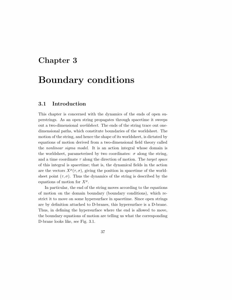
This chapter is concerned with the dynamics of the ends of open su-perstrings. As an open string propagates through spacetime it sweepsout a two-dimensional worldsheet. The ends of the string trace out one-dimensional paths, which constitute boundaries of the worldsheet. Themotion of the string, and hence the shape of its worldsheet, is dictated byequations of motion derived from a two-dimensional field theory calledthe nonlinear sigma model. It is an action integral whose domain isthe worldsheet, parameterised by two coordinates: σ along the string,and a time coordinate τ along the direction of motion. The target spaceof this integral is spacetime; that is, the dynamical fields in the actionare the vectors Xµ(τ, σ), giving the position in spacetime of the world-sheet point (τ, σ). Thus the dynamics of the string is described by theequations of motion for Xµ.
In particular, the end of the string moves according to the equationsof motion on the domain boundary (boundary conditions), which re-strict it to move on some hypersurface in spacetime. Since open stringsare by definition attached to D-branes, this hypersurface is a D-brane.Thus, in defining the hypersurface where the end is allowed to move,the boundary equations of motion are telling us what the correspondingD-brane looks like, see Fig. 3.1.
37

38 CHAPTER 3. BOUNDARY CONDITIONS
Worldsheet
String
D−brane
Figure 3.1: An open string propagating in spacetime sweeps out a two-dimensional
worldsheet. The hypersurface to which its end is confined defines a D-brane.
How restrictive these equations of motion are depends on the amountof symmetry preserved on the boundary. We focus here on the minimally(N=1) supersymmetric conformal nonlinear sigma model,1 assumingthat the worldsheet bulk superconformal symmetry is preserved alsoon the boundary (the D-brane). We showed in Papers II–IV that theboundary conditions allowed by this assumption are more general thanthose commonly used elsewhere — the latter conditions are just specialcases. Nevertheless, we will see that our conditions do impose somerestrictions on the properties of D-branes.
In deriving the boundary equations of motion, the naive approachwould be to do so directly from the action, by use of the principle ofleast action (i.e. a perturbation of the action should vanish). This ishazardous, as the result does not necessarily preserve the desired sym-metries. One could in principle amend this by modifying the actionby extra boundary terms to make it superconformal on the boundary.However, there is no systematic way to find those boundary terms, ex-cept guessing them. In Papers II and III we therefore went for thesafer method of analysing the currents that correspond to the relevantsymmetries, requiring that they be conserved on the boundary. This de-
1In Papers II and IV we also made a sketchy analysis of the N=2 model. In this
case a rich structure arises due to an ambiguity in choice of sign in the boundary
conditions. The N=2 model was studied in more detail in [42, 43].
3.2. THE BOSONIC MODEL 39
fines boundary conditions for the currents, from which we could deriveconditions on the brane.
Having thus obtained the minimal requirements for boundary super-conformal invariance in a general background, it is natural to consider aspecial case of background. In Paper IV we chose the ever popular WZWmodel, which is a nonlinear sigma model defined on a group manifold,with chiral isometry currents [44, 45]. Here our boundary conditions im-ply a surprisingly general gluing map between the isometry currents, thegeometrical implications of which remain unclear at the time of writing.
3.1.1 Outline
To introduce some fundamental concepts pertaining to symmetries andconserved currents, we begin in Section 3.2 by discussing the bosonicnonlinear sigma model. Then we define the supersymmetric sigma modelin Section 3.3, explaining about superspace and superfields, and how toderive the superconformal currents. In Section 3.4 we make an ansatzfor the worldsheet fields which, after introducing some necessary nota-tion in Section 3.5, we plug into the conservation laws for the currentsand obtain in Section 3.6 the complete set of conditions for a super-conformal D-brane, which we interpret in geometrical terms. Promptedby similarities to the structures of almost product manifolds, we look atglobally defined boundary conditions in Section 3.7, drawing some con-clusions about the global embedding of D-branes in spacetime. Finallyin Section 3.8 we apply our analysis to the WZW model, leading to someinteresting statements about gluing maps of group currents.
3.2 The bosonic model
Consider an open string of tension T propagating on a spacetime mani-fold that supports a general background two-tensor Eµν(X) ≡ Gµν(X)+Bµν(X). Here Gµν is the spacetime metric and Bµν an antisymmetricB-field, both of which may depend on the spacetime coordinates Xµ.
40 CHAPTER 3. BOUNDARY CONDITIONS
Then the nonlinear sigma model for the string is (see [46], Section 3.4)
S = −T2
∫dτdσ
[√−g gab∂aX
µ∂bXνGµν(X)
+ εab∂aXµ∂bX
νBµν(X)], (3.1)
where gab is the metric on the worldsheet, g ≡ det gab, and εab is theworldsheet antisymmetric tensor with ετσ=−εστ=1 and εττ = εσσ=0.
One may derive equations of motion for the string by varying (3.1)with respect to Xµ. Since the string is open, the domain of the integralhas boundaries, which contribute boundary terms to the equations ofmotion. The dynamics of the ends of the string is then determined by thevanishing of these boundary terms, implying some nontrivial boundaryconditions for the open string.
The boundary conditions are of two types; either the string is movingfreely along the Xµ-direction — Neumann conditions — or it is stuckin that direction — Dirichlet conditions. The hypersurface to whichthe string’s endpoint is confined, i.e. the D-brane, thus extends alongNeumann directions and is pointlike in Dirichlet directions (see [39],Chapter 8).
However, the boundary equations of motion obtained in this waydo not necessarily preserve all the symmetries that are preserved in thebulk. If our prime concern is that they do (which it is), then we arebetter off analysing conserved currents.
3.2.1 Conserved currents
The model (3.1) is invariant under three different symmetries: spacetimePoincare transformations, worldsheet conformal transformations (rescal-ing of the two-dimensional metric gab), and worldsheet reparameterisa-tion. The last symmetry allows us to switch to lightcone coordinates onthe worldsheet, ξ± ≡ τ ± σ, and we use this basis henceforth.
Each symmetry corresponds to a conserved current, obtained byvarying the action with respect to the appropriate field. The requirementthat the action be invariant under this perturbation (in the bulk) trans-
3.2. THE BOSONIC MODEL 41
lates into a conservation law2 saying that the current is divergence-free,i.e. there are no sources. For example in the case of conformal invari-ance, the corresponding current is the stress energy-momentum tensorand is derived by varying (3.1) with respect to gab. Its components inlightcone coordinates are
T±± = ∂++=Xµ∂
++=XνGµν , (3.2)
where ∂++=
are the derivatives with respect to ξ±, and we have rescaled
the tension to one. The T++ component depends only on ξ+, and iscalled the “left-moving” current, whereas T−− depends only on ξ− andis referred to as “right-moving.” Here the bulk conservation law takesthe form ∂=T++ = ∂++T−− = 0.
To ensure that also the boundary is conformally invariant, we needto impose current conservation on the boundary separately. In generalwe find the boundary condition for a given current Ja
b by using itsassociated charge Qb ≡
∫dσJτ
b. This charge is conserved in the sensethat it is time-independent, ∂τQb = 0 (see [11], Section 3.2). Thus,since Ja
b obeys the conservation law ∂aJab = 0, we may write charge
conservation as
0 = ∂τQb =∫dσ ∂τJ
τb = −
∫dσ ∂σJ
σb = −[Jσ
b ]σ=πσ=0 . (3.3)
Hence we obtain the boundary condition Jσb = 0, for b = τ, σ. Applied
to the stress tensor, the result is
T++ − T−− = 0, (3.4)
i.e. the left- and right-moving components of the stress tensor must beequal. Via the relation (3.2) between the stress tensor and the worldsheetfields, we thus find a boundary condition relating the left-moving fields∂++X
µ to the right-moving fields ∂=Xµ.
In conclusion, we have derived the condition for conformal invarianceon the boundary in the bosonic model. But we are interested in thesupersymmetric theory, which looks a little bit different.
2The conservation law holds only up to equations of motion; we say that it holds
on-shell.
42 CHAPTER 3. BOUNDARY CONDITIONS
3.3 The superspace action
The bosonic model (3.1) has only the three symmetries listed in Sec-tion 3.2. If we want more symmetry the action needs to be modified.In particular, to make it supersymmetric we have to add superpartnerfields that together with the bosonic worldsheet scalars Xµ make upmultiplets (cf. Section 2.3). We thus add two worldsheet spinors ψµ
± andan auxiliary (i.e. nondynamical) field Fµ
+−.The fields constituting a multiplet can be conveniently collected in
a single superfield. The idea is to promote the ordinary worldsheet to asuperspace by supplementing the bosonic worldsheet coordinates ξ± withanticommuting coordinates θ±. Superfields are terminating polynomialsin θ±, with the multiplet fields as coefficients. For example, a multiplet(Xµ, ψµ
±, Fµ+−) would correspond to the superfield [15]
Φµ ≡ Xµ + iθ+ψµ+ + iθ−ψµ
− + θ+θ−Fµ+−.
Similarly, the worldsheet derivatives ∂++=
in (the lightcone version of)(3.1) are extended by additional “superderivatives” D±, and the actionbecomes an integral over superspace rather than over ordinary space.Superspace comes equipped with integration rules that render this inte-gral equivalent to the ordinary one [15].
The whole point of using superfield notation is that the supersym-metric theory can be analysed in a much more compact way than if wewere to use the explicit “component form.” Instead of writing out thekinetic terms in the action for all the multiplet fields individually, we cansimply replace the bosonic fields in (3.1) with superfields. In lightconecoordinates we thus obtain
S =∫d2ξd2θD+ΦµD−ΦνEµν(Φ), (3.5)
where Eµν is the superfield whose lowest component is the backgroundtensor Eµν . Analysis of the superspace action can then be performedin a way completely analogous to the bosonic case, using superspacequantities instead of bosonic ones.
3.3. THE SUPERSPACE ACTION 43
Without boundaries, the action (3.5) is N=(1,1) (globally) super-symmetric, i.e. it is invariant under two independent supersymmetrytransformations that transform the bosonic and fermionic fields into eachother. One is parameterised by a left-moving supersymmetry parameterε+, and the other by a right-moving one, ε−. These two parameters area priori independent of each other, and each of them is associated witha conserved supersymmetry current; we denote these currents by G±.
In the presence of a boundary the supersymmetry parameters andcurrents are subject to boundary conditions that relate left- and right-movers, as we saw in Section 3.2. The supersymmetry parameters be-come identified up to a sign, ε+ = ηε− (η ≡ ±1), reducing the N=(1,1)symmetry to N=1. For the currents the boundary condition (3.3) is
G+ − ηG− = 0, (3.6)
which is the condition for the boundary to preserve worldsheet super-symmetry.
The condition (3.6) together with the stress tensor condition (3.4)define the superconformal boundary conditions for the classical opensuperstring. It is these two conditions that served as our starting pointin Papers II–IV. To derive the corresponding boundary conditions forthe worldsheet fields we need to write the currents T±± and G± in termsof Xµ and ψµ
±. In the bosonic theory the expression for the stress tensorwas (3.2); here the relation is more complicated, involving also ψµ
±. Wenow briefly explain how to compute the superconformal currents from alocally supersymmetric sigma model.
3.3.1 Finding the currents
The conformal and supersymmetry currents can be viewed as com-ponents of a superfield which we call the “supercurrent,” and whichwe denote by T B
A (the indices A,B run over the superspace indices++,=,+,−). This is a kind of stress tensor for a locally supersymmetricversion of the nonlinear sigma model (3.5).
What one does is to “gauge” the model by replacing the flat su-perderivatives D± with covariant ones, ∇±, as well as introducing a
44 CHAPTER 3. BOUNDARY CONDITIONS
supervielbein3 E AM on superspace (see [46], Section 4.3.4). The action
then becomes
S =∫d2ξd2θ E ∇+Φµ∇−Φν Eµν(Φ),
where E is the determinant of the supervielbein.Next we vary S with respect to the vielbein components and ob-
tain the supercurrent, of which only two components do not vanish on-shell, namely T −
++ and T += [48]. These are expressions in covariant
superderivatives of superfields, and we revert to global supersymmetryby replacing the covariant derivatives with flat ones again. Finally, wecan extract the components of the supercurrent as follows,
G+ = T −++ |, G− = T +
= |,
T++ = −iD+T−
++ |, T−− = −iD−T += |.
The result is a set of explicit expressions for the currents in terms ofworldsheet fields, which we omit here; they are given in Paper III.
It is now in principle straightforward to convert the boundary con-ditions (3.4) and (3.6) for the currents into boundary conditions for thefields Xµ and ψµ
±. We know that the boundary enforces relations be-tween left- and right-movers, so we can make an ansatz for the way inwhich the left- and right-moving worldsheet fields are related to eachother, and then derive restrictions on this ansatz from the current con-ditions. Thus our plan of attack is to make the most general ansatzpossible for the worldsheet fields, plug it into the current conditions,and reduce these conditions to an independent set of boundary condi-tions that we can interpret.
3.4 The ansatz
It turns out that the most general, local ansatz we can make in ourclassical conformal theory is very simple for the fermions, due to the
3Vielbeins are orthonormal tangent vectors that may be used to go to a locally
flat tangent space at a point (see [47], Chapter 12).
3.4. THE ANSATZ 45
absence of dimensionful parameters. We therefore start with this ansatzand then derive the corresponding bosonic relation by a supersymmetrytransformation. A little dimensional analysis reveals that the fermionicansatz takes the form (the sign η = ±1 is included merely for conve-nience)
ψµ− = ηRµ
ν(X)ψν+, (3.7)
where Rµν is a general (1,1)-tensor defined on the boundary, which may
depend on the worldsheet scalar Xµ at that point, but not on ψµ±. The
bosonic superpartner of (3.7) is more complicated,
∂=Xµ −Rµ
ν∂++Xν + 2i(P σ
ρ∇σRµν + Pµ
γGγδHδσρR
σν)ψ
ρ+ψ
ν+ = 0, (3.8)
where we have defined 2Pµν ≡ δµ
ν +Rµν (δµ
ν is the Kronecker delta), theantisymmetric three-tensor Hµνρ is the field strength (or torsion) of thebackground B-field, and ∇σ is the Levi-Civita connection. Note that(3.8) is more general than the usual boundary conditions adopted inthe literature (see e.g. [49]), in that there is an extra two-fermion termallowed by superconformal invariance.4 We showed in Papers II and IIIthat this extra term vanishes only for very special cases.
The ansatz (3.7) encodes in a covariant form the standard Neumannand Dirichlet boundary conditions that define a D-brane. In the pres-ence of a B-field the Neumann condition has an a priori very generalform, while the Dirichlet condition is much simpler. If we choose a basiswhere the worldvolume coordinates of the D-brane are aligned with thespacetime coordinates — called adapted coordinates — then the Dirich-let condition takes the familiar form
∂τXi = 0, (3.9)
stating that the position of the endpoint along the i:th Dirichlet directiondoes not change with worldsheet time τ , i.e. it is frozen in that direction.The corresponding situation holds for the spinors,
ψi− = −η ψi
+. (3.10)4But see also [50], where an extra two-fermion term is included.
46 CHAPTER 3. BOUNDARY CONDITIONS
At first glance Rµν seems a completely general object, but we can ac-
tually say something about it already at this stage, by going to adaptedcoordinates at a point. In this basis it should imply (3.10), so theDirichlet-Dirichlet part is Ri
j = −δij. On the other hand, the Neu-
mann condition is still very general (m,n label Neumann directions),
ψm− = ηRm
n(X)ψn+, (3.11)
for some Neumann-Neumann tensor Rmn. It is clear that this tensor
depends on the B-field, because for Bµν = 0 we expect (3.11) to reduceto ψm− = η ψm
+ . In fact, one may think of Rmn as defining the B-field;5
we will see later precisely how.To summarise, if we write Rµ
ν as a 2×2 block matrix, with the up-per left block being the Neumann-Neumann part, the lower right theDirichlet-Dirichlet part, and the off-diagonal blocks the mixed parts, wehave
Rµν =
(Rm
n 00 −δi
j
). (3.12)
But we want to work in a basis-independent notation, so we wouldlike to write for example the Dirichlet condition (3.9) in a covariantform.6 To do this, we need to introduce some structures on our spacetimemanifold. These structures are natural from a physical point of view,but there is a rich mathematical machinery associated with them, whichwill be tremendously useful in writing down and interpreting the finalboundary conditions.
3.5 Structures on D-branes
We begin by defining a projector Qµν on the worldsheet boundary, which
projects vectors on the D-brane onto the space spanned by the Dirichletdirections. That is, given a vector Xµ at some point on the brane, Qµ
νXν
is by definition normal to the brane at that point. If Xµ is invariant5Note that Bµν is actually the gauge invariant combination of a truly background
B-field and the field strength of the U(1) gauge field on the D-brane.6We focus on the Dirichlet condition because of its simple form.
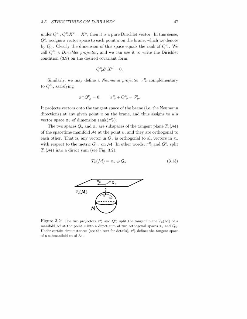
3.5. STRUCTURES ON D-BRANES 47
under Qµν , Q
µνXν = Xµ, then it is a pure Dirichlet vector. In this sense,
Qµν assigns a vector space to each point u on the brane, which we denote
by Qu. Clearly the dimension of this space equals the rank of Qµν . We
call Qµν a Dirichlet projector, and we can use it to write the Dirichlet
condition (3.9) on the desired covariant form,
Qµν∂τX
ν = 0.
Similarly, we may define a Neumann projector πµν complementary
to Qµν , satisfying
πµνQ
νρ = 0, πµ
ν +Qµν = δµ
ν .
It projects vectors onto the tangent space of the brane (i.e. the Neumanndirections) at any given point u on the brane, and thus assigns to u avector space πu of dimension rank(πµ
ν).The two spaces Qu and πu are subspaces of the tangent plane Tu(M)
of the spacetime manifold M at the point u, and they are orthogonal toeach other. That is, any vector in Qu is orthogonal to all vectors in πu
with respect to the metric Gµν on M. In other words, πµν and Qµ
ν splitTu(M) into a direct sum (see Fig. 3.2),
Tu(M) = πu ⊕Qu. (3.13)
πu
Tuu
Qu
( )m
Figure 3.2: The two projectors πµν and Qµ
ν split the tangent plane Tu(M) of a
manifold M at the point u into a direct sum of two orthogonal spaces πu and Qu.
Under certain circumstances (see the text for details), πµν defines the tangent space
of a submanifold m of M.
48 CHAPTER 3. BOUNDARY CONDITIONS
It is worth emphasising that the only assumption we make from theoutset is that the target space is a smooth manifold equipped with a(pseudo-) Riemannian metric and an antisymmetric two-tensor (the B-field). A priori we do not know anything about the properties of theD-brane; it need not be a regular submanifold of spacetime, and couldbe singular or ill-defined for all we know. Our object is to start from thisunassuming standpoint and derive the properties required of the braneby superconformal invariance. It is thus by no means certain at thispoint that πµ
ν defines a tangent space corresponding to a submanifoldof spacetime, although the vector space πu is a subspace of Tu(M).However, we will see in Section 3.7 that, under certain circumstances,this follows as a consequence of the superconformal boundary conditions.
We need one more object before writing down the boundary con-ditions. Given two orthogonal projectors πµ
ν and Qµν we may define
another (1,1)-tensor,rµ
ν ≡ πµν −Qµ
ν ,
which squares to the identity, rµνrν
ρ = δµρ, since πµ
ν and Qµν are orthog-
onal and each of them squares to itself. Alternatively, πµν and Qµ
ν canbe written in terms of rµ
ν ,
πµν =
12
(δµν + rµ
ν) , Qµν =
12
(δµν − rµ
ν) .
The three structures πµν , Q
µν and rµ
ν , although very simple and in-tuitive in essence, were crucial in deriving and understanding the super-conformal boundary conditions in Papers II and III. Note that initiallythey are defined only at a point, the endpoint of the string. However,we will see that superconformal invariance allows us to extend themto a neighbourhood, thus providing some information about the localsmoothness of the brane. In fact, we will even define them globally (i.e.at every point inM), just to see what happens. One can then draw someconclusions about the way in which the D-brane is embedded, globally,in spacetime, rather than merely looking at a small coordinate patch ofthe brane. But before exploring such possibilities, let us finally writedown the boundary conditions explicitly.
3.6. THE BOUNDARY CONDITIONS 49
3.6 The boundary conditions
Using the ansatz (3.7) and (3.8) in the current conditions (3.4) and (3.6),we found in Paper III the following three boundary conditions,
RµρGµνR
νσ = Gρσ, (3.14)
πρσEνρπ
νγ = πρ
σEρνπνλR
λγ , (3.15)
πρσπ
νλ∇[ρQ
µν] = 0. (3.16)
We also showed that they make up a complete set, i.e. there are nofurther independent conditions to be found.
It may seem that these conditions are not in fact conditions on theworldsheet fields, which we claimed we were after. However, they areexplicit conditions on the structures on the brane, which is equivalentto restrictions of the motion of the string endpoints.
The first condition says that the boundary map Rµν preserves the
spacetime metric. This implies that the metric diagonalises so that itconsists of a Neumann-Neumann part and a Dirichlet-Dirichlet part, buthas no “mixed” components. One may see how this happens by goingto adapted coordinates; there we have seen that Rµ
ν has the diagonalform (3.12), so it follows immediately from (3.14) that the metric mustbe block-diagonal, Gµν = diag(Gmn, Gij).
There are two things to note here. First, the diagonal form of themetric does not necessarily imply that the two constituent blocks arecompletely decoupled. There may still be interdependence such that e.g.Gmn depends on Dirichlet coordinates. Second, it is important to realisethat the condition (3.14) is not imposing restrictions on the spacetimemetric, but on the D-brane — its embedding in target space must besuch that the metric diagonalises.
Moving on to the second boundary condition, Eq. (3.15), we seethat it is a condition on the Neumann-Neumann part of Rµ
ν . It is essen-tially the definition of the B-field mentioned in Section 3.4; in adaptedcoordinates it schematically looks like E−1ET = R (along the Neumann-Neumann directions). From this form we can derive the behaviour ofthe string for large B-field; as we take B →∞, the Neumann-Neumann
50 CHAPTER 3. BOUNDARY CONDITIONS
block of Rµν goes to −δm
n, i.e. we find that the Neumann conditions turninto Dirichlet conditions. That is, the endpoint of the string is com-pletely frozen in all directions in this limit. It is also interesting to notethat, in the limit B → 0, we find Rµ
ν → rµν .
Last but not least, we want to interpret the condition (3.16). This isactually a precise mathematical statement saying that the projector πµ
ν
is integrable [51]. There are several ways of understanding the contentof this statement [52], but perhaps the most intuitive one is to considertwo displacements along the Neumann directions. If the commutator[δ1, δ2]Xµ between them vanishes, then regardless of which order we dothem in, we always end up in the same point. If, on the other hand,they do not commute, the final position will depend on the order ofdisplacement. The latter case corresponds to some singular D-braneabout which we cannot say much. The former situation, however, is theinteresting one, because it occurs if and only if (3.16) holds, as is easilyseen by inserting δXµ = πµ
νδXν in the commutator. It implies localsmoothness at the point u in the sense that we can extend the basis ofπu to a neighbourhood of u [53]. In particular the adapted coordinatebasis, where πµ
ν takes the form
πµν =
(δm
n 00 0
), (3.17)
can be extended to a neighbourhood of u so that πµν is given by (3.17)
on the whole neighbourhood.7 And since we can define Qµν wherever
πµν is defined, and hence rµ
ν , it follows that we may extend all three ofour (1,1)-tensors to a neighbourhood of u.
Another consequence of π-integrability is that the Neumann-Neumannpart of the metric is independent of the Dirichlet directions [52] (thoughas long as Qµ
ν is not integrable, the Dirichlet-Dirichlet part of Gµν maystill depend on the Neumann coordinates).
This is as far as we get in our interpretation of the conditions (3.14)–(3.16) without making additional assumptions. But the properties of our
7Note that this extension is only possible along the Neumann directions. If Qµν
were integrable too, then we would be able to extend the basis in all directions.
3.7. GLOBALLY DEFINED CONDITIONS 51
structuresQµν , π
µν and rµ
ν are exactly the same as those of the structuresassociated with almost product manifolds [52], except that they are notglobally defined. We therefore found it irresistible to add this extraproperty in Papers II and III, and investigate the consequences.
3.7 Globally defined conditions
By “globally defined” we mean that our structures Qµν , π
µν and rµ
ν , aswell as Rµ
ν , all are defined not only at a point u (and, by integrability,on a neighbourhood of u), but at every point v in spacetime.
In this case, πµν and Qµ
ν are distributions on M [51]. That is, theyassign a space of vectors (πv and Qv, respectively) to each point v ∈M,thus splitting the whole tangent space T (M) (not just the tangent planeat a point u, cf. Eq. (3.13)) into a direct sum,
T (M) = π ⊕Q. (3.18)
The tensor rµν is now an almost product structure, defining the target
space as an almost product manifold [52]. The word “almost” refers tothe fact that the manifold is not necessarily a direct product, despite itstangent space being a direct sum.8 An example of such a manifold is alocally product manifold, i.e. a manifold that locally looks like a directproduct but globally is not (think of the Mobius strip).
Let us have a fresh look at the boundary conditions (3.14)–(3.16)through our “global glasses.” We saw in Section 3.6 that the first con-dition implies that the metric diagonalises. In adapted coordinates itis then easily seen that the metric preserves also the almost productstructure, since the latter takes the form
rµν =
(δm
n 00 −δi
j
)
in this basis. Thus the spacetime manifold is an almost product manifoldwith a (pseudo-) Riemannian metric that is preserved by the almost
8The failure of the split (3.18) to split M into a direct product is measured by the
Nijenhuis tensor Nρµν ≡ rγ
µrρ[ν,γ] − rγ
νrρ[µ,γ] [54].

52 CHAPTER 3. BOUNDARY CONDITIONS
product structure; such a manifold is called a (pseudo-) Riemannianalmost product manifold [52].
The second boundary condition, Eq. (3.15), gives no new informa-tion, so we turn directly to the condition (3.16), which says that πµ
ν isan integrable distribution. Such an object is by definition a foliation[53, 55]. This means that, at every point v in spacetime, πµ
ν locallydefines, on a neighbourhood of v, a set of hyperplanes, or leaves, thatin adapted coordinates are described by the system of equations Xi=constant [55]. These hyperplanes are contained in the space πv, buta priori need not be of the same dimension, so they are not necessar-ily D-branes (recall that πµ
ν defines the dimensionality of the D-brane).However, there is a theorem by Frobenius saying that when πµ
ν is a fo-liation, then through every point v ∈ M there is a unique submanifoldof M whose tangent space is πv (called a maximal integral manifold ofπµ
ν) [56]; this is the D-brane we were looking for.In conclusion, globally defined superconformal boundary conditions
imply that spacetime is foliated by D-branes which are submanifoldsembedded in such a way that spacetime may be viewed as a (pseudo-)Riemannian almost product manifold. Let us give some concrete exam-ples of such D-brane embeddings.
3.7.1 Examples
As we mentioned above, the obvious special case of an almost productmanifold is a direct product, e.g. a torus (a direct product of one-cycles).Thus, if spacetime were a torus, the superconformally allowed D-braneswould be those that wrap one or more of the constituent one-cycles.
More interestingly, many exact solutions of Einstein’s equations arealmost product manifolds, e.g. the Schwarzschild and Robertson-Walkerspaces. To be explicit, we take a closer look at the Schwarzschild space;it makes an instructive example of the way different D-brane embeddingsdetermine the type of the spacetime manifold.
The Schwarzschild metric is
ds2 = −f(r)dt2 + h(r)dr2 + r2dΩ2, (3.19)
3.8. THE WZW MODEL 53
where t is time, r is the radial coordinate, f(r) ≡ 1−M/r with M a con-stant, h(r) ≡ 1/f(r), and dΩ2 is the metric on a two-sphere. Assumingthat t is the time coordinate also on the worldvolume of the D-brane,there is only one embedding which is allowed by the superconformalboundary conditions (3.14)–(3.16). We can write the manifold at handas a warped product manifold
(M1 ×M2 , G1(t, r)⊕ r2G2(Ω2) ),
withG1(t, r) ≡ −f(r)dt2+h(r)dr2 being the metric onM1 andG2(Ω2) ≡dΩ2 the metric on M2. It is called “warped” because the factor in frontof G2 (in our case r2) depends on the coordinates of M1. Then thebrane can extend along t and r, i.e. we have a D1-brane that coincideswith the manifold M1. Here G1(t, r) is the metric on the brane; it is in-dependent of the M2-coordinates, which is consistent with integrabilityof πµ
ν . On the other hand, there is a problem with integrability at thesingularity r = 0; nevertheless, the general principle should be clear.
Alternatively, we may write the metric (3.19) as a different almostproduct manifold,
(M1 ×M2 , G1(t, r,Ω2)⊕G2(r) ),
with G1(t, r,Ω2) ≡ −f(r)dt2 + r2dΩ2 and G2(r) ≡ h(r)dr2. Here wecould have a D2-brane wrapping M1. However, it would not be su-perconformal, since πµ
ν is not integrable in this case; the Neumann-Neumann metric G1(t, r,Ω2) depends on the Dirichlet direction r. Fi-nally, there is also the possibility of a D0-brane, extending only along t,in which case spacetime again is a warped product manifold, with warpfactor −f(r). Also this brane breaks superconformal invariance, sincethe metric on the brane depends on the Dirichlet directions.
The various embeddings are illustrated in Fig. 3.3.
3.8 The WZW model
In the preceding sections we have learnt the minimal requirements for aD-brane to preserve superconformal symmetry in a general spacetime.
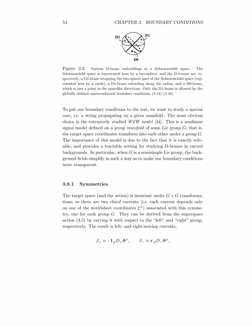
54 CHAPTER 3. BOUNDARY CONDITIONS
D2 D1
D0
Figure 3.3: Various D-brane embeddings in a Schwarzschild space. The
Schwarzschild space is represented here by a two-sphere, and the D-branes are, re-
spectively, a D2-brane wrapping the two-sphere part of the Schwarzschild space (rep-
resented here by a circle), a D1-brane extending along the radius, and a D0-brane,
which is just a point in the spacelike directions. Only the D1-brane is allowed by the
globally defined superconformal boundary conditions (3.14)–(3.16).
To put our boundary conditions to the test, we want to study a specialcase, i.e. a string propagating on a given manifold. The most obviouschoice is the extensively studied WZW model [44]. This is a nonlinearsigma model defined on a group manifold of some Lie group G; that is,the target space coordinates transform into each other under a group G.The importance of this model is due to the fact that it is exactly solv-able, and provides a tractable setting for studying D-branes in curvedbackgrounds. In particular, when G is a semisimple Lie group, the back-ground fields simplify in such a way as to make our boundary conditionsmore transparent.
3.8.1 Symmetries
The target space (and the action) is invariant under G×G transforma-tions, so there are two chiral currents (i.e. each current depends onlyon one of the worldsheet coordinates ξ±) associated with this symme-try, one for each group G. They can be derived from the superspaceaction (3.5) by varying it with respect to the “left” and “right” group,respectively. The result is left- and right-moving currents,
J+ ≡ −l µD+Φµ, J− ≡ r µD−Φµ,
3.8. THE WZW MODEL 55
where l µ and r µ are the superfield Killing vectors associated with eachsymmetry. We denote the lowest (fermionic) components of J± by
j+ ≡ J+| = −lµψµ+, j− ≡ J−| = rµψ
µ−, (3.20)
where lµ and rµ are the lowest components of the superfield Killingvectors.9
The vectors lµ and rµ can be expanded in the Lie algebra basis TAof their corresponding groups, as lµ ≡ lµAT
A and rµ ≡ rµAT
A. Then thecoefficients lµA and rµ
A satisfy the corresponding Lie algebra,
[lA, lB ] = −f CAB lC , [rA, rB ] = f C
AB rC
(the sign is just a convention), and they commute with each other,[lA, rB ] = 0. Here the Lie bracket for vectors vµ
A is defined as [vA, vB ]µ ≡vν
A∂νvµB − vν
B∂νvµA.
3.8.2 The gluing map
From (3.20) follows immediately that the fermionic ansatz (3.7) trans-lates into a boundary condition for the group currents,
jA− = η RAB j
B+ ,
whereRA
B ≡ −lAµRµνr
νB . (3.21)
The transformation in (3.21) is essentially a change of basis from space-time vectors to the Lie algebra basis [45].
The object RAB is a gluing map between the chiral currents at the
worldsheet boundary. Since it maps jB+ to jA−, which are elements of theLie algebra, it is clearly a map from the Lie algebra into itself. Whatmore we can say about this map? It is usually assumed in the literatureto be a constant Lie algebra automorphism [45, 57, 58]. This means thatit preserves the Lie algebra structure in the sense that[
RCATC , R
DBTD
]= f C
AB RFCTF . (3.22)
9The vector rµ should not be confused with the almost product structure rµν in
Section 3.7.
56 CHAPTER 3. BOUNDARY CONDITIONS
However, this restriction is always made for practical reasons, as a non-constant gluing map makes the quantum theory unwieldy. And indeedwe found in Paper IV that RA
B in the N=1 model can in principle be amuch more general object.
To see how we reach this conclusion, let us write down the boundaryconditions for the WZW model. For this purpose, we take advantage ofthe fact that on group manifolds the metric and torsion can be expressedentirely in terms of Killing vectors, Lie algebra structure constants andthe Cartan-Killing metric10 ηAB [59]. As a consequence, the boundaryconditions (3.14) and (3.16) can be written as equations involving onlythese quantities plus RA
B , and we end up with the following conditions,
ηAB = RCAηCDR
DB , (3.23)
fABC − fDEFRDAR
EBR
FC = ηDER
D[A
(LCR
EB]
). (3.24)
Here the Lie derivative is defined as
LCREB ≡ LrC
REB −RH
CLlHREB =
(rµC −RH
C lµH
)RE
B,µ,
with LrCthe usual Lie derivative with respect to the vector rµ
C .The first condition, Eq. (3.23), says that the gluing map preserves the
Cartan-Killing metric. But it is the second condition, Eq. (3.24), thatinterests us. To see what it means, let us first use (3.23) to manipulatethe Lie bracket (3.22) a little. We can rewrite the left-hand side of (3.22)as
RDAR
EB [TD, TE ] = RD
AREBf
FDE TF ,
whence, using (3.23), follows that RAB is a Lie algebra automorphism if
and only iffABC − fDEFR
DAR
EBR
FC = 0.
Thus we see that RAB is a Lie algebra automorphism if and only if the
right-hand side of (3.24) vanishes.Hence we draw two conclusions from (3.24). First, RA
B does nothave to be a Lie algebra automorphism. Second, it can be a Lie algebra
10The Cartan-Killing metric is defined as ηAB ≡ −f DAC f C
BD .
3.8. THE WZW MODEL 57
automorphism without being constant, since the right-hand side canvanish even if RA
B is nonconstant. The interpretation of this conditionin terms of D-branes was not addressed in Paper IV, but it is knownthat for the special case where RA
B is constant, conformally invariantD-branes are obtained as conjugacy classes of the group G [57].

58 CHAPTER 3. BOUNDARY CONDITIONS
Bibliography
[1] A. Bilal, Higher-derivative corrections to the non-abelian Born-Infeld action, Nucl. Phys. B618 (2001) 21-49, hep-th/0106062.
[2] P. Koerber and A. Sevrin, The non-abelian D-brane effective ac-tion through order α′4, JHEP 0210 (2002) 046, hep-th/0208044.
[3] B. R. Greene, String Theory on Calabi-Yau Manifolds, TASI lec-ture notes (1996), hep-th/9702155.
[4] P. S. Aspinwall, K3 surfaces and string duality, TASI lecturenotes (1996), hep-th/9611137.
[5] J. Polchinski, String theory, Vol II (Cambridge University Press,1998).
[6] K. Intriligator and N. Seiberg, Mirror Symmetry in Three Di-mensional Gauge Theories, Phys. Lett. B387 (1996) 513-519,hep-th/9607207.
[7] P. B. Kronheimer, The construction of ALE spaces as Hyper-Kahler quotients, J. Diff. Geom. 29 (1989) 665.
[8] U. Lindstrom, M. Rocek and R. von Unge, Hyperkahler quotientsand algebraic curves JHEP 0001 (2000) 022, hep-th/9908082.
[9] I. Y. Park and R. von Unge, Hyperkahler quotients, mirror sym-metry, and F-theory, JHEP 0003 (2000) 037, hep-th/0001051.
59
60 BIBLIOGRAPHY
[10] W. Fulton and J. Harris, Representation Theory: A First Course(Springer-Verlag, 1991).
[11] L. H. Ryder, Quantum field theory (Cambridge University Press,1996).
[12] M. Maggiore, Champs et Particules, Chapter 9, lecture notes2001/02, Departement de Physique Theorique de l’Universite deGeneve.
[13] A. Bilal, Duality in N=2 susy SU(2) Yang-Mills theory: A ped-agogical introduction to the work of Seiberg and Witten, hep-th/9601007.
[14] C. V. Johnson and R. C. Myers, Aspects of Type IIB theory onALE spaces, Phys. Rev. D55 (1997) 6382-6393, hep-th/9610140.
[15] J. Wess and J. Bagger, Supersymmetry and supergravity (Prince-ton University Press, 1992).
[16] P. S. Aspinwall, Compactification, geometry and duality: N=2,TASI lecture notes (1999), hep-th/0001001.
[17] N. J. Hitchin, A. Karlhede, U. Lindstrom and M. Rocek, Hy-perkahler metrics and supersymmetry, Commun. Math. Phys.108 (1987) 535-589.
[18] W. Lerche, Introduction to Seiberg-Witten theory and its stringyorigin, Nucl. Phys. Proc. Suppl. 55B (1997) 83-117; Fortsch.Phys. 45 (1997) 293-340, hep-th/9611190.
[19] N. Seiberg and E. Witten, Monopole condensation and confine-ment in N=2 supersymmetric Yang-Mills theory, Nucl. Phys.B426 (1994) 19-52; Erratum-ibid. B430 (1994) 485-486, hep-th/9407087.
[20] P. C. Argyres, M. R. Plesser and N. Seiberg, The moduli space ofN=2 SUSY QCD and duality in N=1 SUSY QCD, Nucl. Phys.B471 (1996) 159-194, hep-th/9603042.
BIBLIOGRAPHY 61
[21] N. Koblitz, Introduction to elliptic curves and modular forms,2nd ed. (Springer-Verlag, 1993).
[22] K. Kodaira, On compact analytic surfaces, II-III, Ann. of Math.77 (1963) 563; 78 (1963) 1.
[23] P. C. Argyres, M. R. Plesser, N. Seiberg and E. Witten, New N=2superconformal field theories in four dimensions, Nucl. Phys.B461 (1996) 71, hep-th/9511154.
[24] T. Eguchi, K. Hori, K. Ito and S.-K. Yang, Study of N=2 su-perconformal field theories in 4 dimensions, Nucl. Phys. B471(1996) 430, hep-th/9603002.
[25] J. Minahan and D. Nemeschansky, An N=2 superconformal fixedpoints with E6 global symmetry, Nucl. Phys. B482 (1996) 142-152, hep-th/9608047.
[26] J. Minahan and D. Nemeschansky, Superconformal fixed pointswith En global symmetry, Nucl. Phys. B489 (1997) 24-46, hep-th/9610076.
[27] M. Noguchi, S. Terashima and S.-K. Yang, N=2 superconformalfield theory with ADE global symmetry on a D3-brane probe, Nucl.Phys. B556 (1999) 115-151, hep-th/9903215.
[28] N. Seiberg, Five dimensional SUSY field theories, non-trivialfixed points and string dynamics, Phys. Lett. B388 (1996) 753-760, hep-th/9608111.
[29] W. Lerche and N. P. Warner, Exceptional SW geometry fromALE fibrations, Phys. Lett. B423 (1998) 79-86, hep-th/9608183.
[30] C. Vafa, Evidence for F-Theory, Nucl. Phys. B469 (1996) 403-418, hep-th/9602022.
[31] A. Johansen, A comment on BPS states in F-theory in 8 dimen-sions, Phys. Lett. B395 (1997) 36, hep-th/9608186.
62 BIBLIOGRAPHY
[32] M. R. Gaberdiel and B. Zwiebach, Exceptional groups from openstrings, Nucl. Phys. B518 (1998) 151-172, hep-th/9709013.
[33] T. Banks, M. Douglas and N. Seiberg, Probing F-theory withbranes, Phys. Lett. B387 (1996) 278, hep-th/9605199.
[34] A. Fayyazuddin and M. Spalinski, The Seiberg-Witten differ-ential from M-Theory, Nucl. Phys. B508 (1997) 219-228, hep-th/9706087.
[35] O. Aharony, A. Fayyazuddin and J. Maldacena, The large N limitof N = 2, 1 field theories from threebranes in F-theory, JHEP9807 (1998) 013, hep-th/9806159.
[36] A. Sen, F-theory and orientifolds, Nucl. Phys. B475 (1996) 562-578, hep-th/9605150.
[37] B. Feng, A. Hanany, Y.-H. He and N. Prezas, Stepwise projection:toward brane setups for generic orbifold singularities, JHEP 0201(2002) 040, hep-th/0012078.
[38] M. Douglas and G. Moore, D-branes, quivers, and ALE instan-tons, hep-th/9603167.
[39] J. Polchinski, String theory, Vol I (Cambridge University Press,1998).
[40] D. Mumford and J. Fogarty, Geometric invariant theory(Springer, 1982).
[41] C. Albertsson, B. Brinne, U. Lindstrom, M. Rocek andR. von Unge, ADE-quiver theories and mirror symmetry, Nucl.Phys. B Proc. Suppl. 102 & 103 (2001) 3-10, hep-th/0103084.
[42] U. Lindstrom and M. Zabzine, N=2 boundary conditions for non-linear sigma models and Landau-Ginzburg models, JHEP 0302(2003) 006, hep-th/0209098.
BIBLIOGRAPHY 63
[43] U. Lindstrom and M. Zabzine, D-branes in N=2 WZW models,to appear in Phys. Lett. B, hep-th/0212042.
[44] K. Gawedzki, Conformal field theory: a case study, hep-th/9904145.
[45] S. Stanciu, D-branes in group manifolds, JHEP 0001 (2000) 025,hep-th/9909163.
[46] M. B. Green, J. H. Schwarz and E. Witten, Superstring theory,Vol I (Cambridge University Press, 1987).
[47] M. B. Green, J. H. Schwarz and E. Witten, Superstring theory,Vol II (Cambridge University Press, 1987).
[48] F. Bastianelli and U. Lindstrom, Induced chiral supergravities in2D, Nucl. Phys. B416 (1994) 227, hep-th/9303109.
[49] H. Ooguri, Y. Oz and Z. Yin, D-branes on Calabi-Yau spaces andtheir mirrors, Nucl. Phys. B477 (1996) 407-430, hep-th/9606112.
[50] E. Alvarez, J. L. F. Barbon and J. Borlaf, T-duality for openstrings, Nucl. Phys. B479 (1996) 218-242, hep-th/9603089.
[51] K. Yano, Differential geometry on complex and almost complexspaces (Pergamon, Oxford, 1965).
[52] K. Yano and M. Kon, Structures on manifolds, Series in PureMathematics, Vol 3 (World Scientific, Singapore, 1984).
[53] B. L. Reinhart, Differential geometry of foliations (Springer-Verlag, 1983).
[54] A. Borowiec, M. Ferraris, M. Francaviglia and I. Volovich, Almostcomplex and almost product Einstein manifolds from a variationalprinciple, J. Math. Phys. 40 (1999) 3446-3464, dg-ga/9612009.
[55] P. Tondeur, Foliations on Riemannian manifolds (Springer-Verlag, New York, 1988).
64 BIBLIOGRAPHY
[56] W. M. Boothby, An introduction to differentiable manifolds andRiemannian geometry (Academic Press, London, 1986).
[57] A. Y. Alekseev and V. Schomerus, D-branes in the WZW model,Phys. Rev. D60 (1999) 061901, hep-th/9812193.
[58] T. Itoh and S.-J. Sin, A note on singular D-branes in group man-ifolds, Nucl. Phys. B650 (2003) 497-521, hep-th/0206238.
[59] C. M. Hull and B. Spence, The gauged nonlinear sigma modelwith Wess-Zumino term, Phys. Lett. B232 (1989) 204.


