Embed Size (px)
Citation preview
arX
iv:h
ep-t
h/05
0901
2v2
15
Sep
2005
DAMTP-2005-78
hep-th/0509012
Kahler Moduli Inflation
Joseph P. Conlon 1 and Fernando Quevedo 2
DAMTP, Centre for Mathematical Sciences,
Wilberforce Road, Cambridge, CB3 0WA, UK
Abstract
We show that under general conditions there is at least one natural
inflationary direction for the Kahler moduli of type IIB flux compactifi-
cations. This requires a Calabi-Yau which has h2,1 > h1,1 > 2 and for
which the structure of the scalar potential is as in the recently found ex-
ponentially large volume compactifications. We also need - although these
conditions may be relaxed - at least one Kahler modulus whose only non-
vanishing triple-intersection is with itself and which appears by itself in
the non-perturbative superpotential. Slow-roll inflation then occurs with-
out a fine tuning of parameters, evading the η problem of F-term inflation.
In order to obtain COBE-normalised density perturbations, the stabilised
volume of the Calabi-Yau must be O(105 − 107) in string units, and the
inflationary scale Minfl ∼ 1013 GeV. We find a robust model independent
prediction for the spectral index of 1− 2Ne
= 0.960 → 0.967, depending on
the number of efoldings.
1e-mail: [email protected]: [email protected]
1 Introduction
One of the most exciting recent developments in string theory has been the greatprogress made in moduli stabilisation [1, 2]. There are now well-establishedtechniques to give masses to the moduli that appear ubiquitously in string com-pactifications. The process of moduli stabilisation represents ‘step zero’ towardsstring phenomenology, as the moduli vevs determine such basic quantities as thestring scale and the gauge coupling constants.
Given moduli potentials, an obvious application is to inflation. While themoduli sector has only indirect effects on Standard Model matter, the dynamicsof light scalar fields is the principal theme of inflation. Inflation is the dominantparadigm for structure formation in the early universe and observations can nowprovide precision tests of inflationary models [3].
In string theory there are several candidates for the inflaton field, which canbe classified according to their origin in either the open or closed string sector[4, 5]. The most common open string inflaton is a brane/antibrane separation[6, 7, 8], whereas closed string inflatons typically correspond to geometric moduli[9]. There has been much recent effort devoted to inflationary model building,particularly since the appearance of the KKLT scenario of moduli stabilisation[2]. For recent discussions, [9, 10, 11, 12] may be consulted.
A standard problem bedevilling both brane and modular inflation - and indeedmost supergravity inflation scenarios - is the η problem. This states that for F-term inflation the slow-roll η parameter is O(1) unless a finely tuned cancellationoccurs. The η problem is manifest for F-term modular inflation. In brane inflationit is not manifest, but reappears once this is embedded into a moduli stabilisationscenario [10].
In this note we will present a simple inflationary scenario within the frameworkof the moduli stabilisation mechanism of [13, 14]. The inflaton is one of theKahler moduli and inflation proceeds by reducing the F-term energy. The η
problem is evaded by the pseudo-no scale property of the Kahler potential. Thestructure of the potential is such that inflation is obtained naturally and almostinevitably, without either fine tuning or a need to introduce large flux or branenumbers. This mechanism in principle applies to a very large class of Calabi-Yaucompactifications that will be specified below.
2 Almost Flat Directions
2.1 General Idea
Slow-roll inflation requires the presence of almost flat directions in the scalarpotential. A natural source of such a flat direction would be a field only appearingexponentially in the potential. Denoting this field by τ , an appropriate (and
2
textbook [15]) potential would be
Vinf = V0
(
1 − Ae−τ + . . .)
, (1)
where the dots represent higher exponents.In string theory there are many moduli whose stabilisation requires nonpertur-
bative effects. Examples are the Kahler moduli in IIB flux compactifications andboth dilaton and Kahler moduli in heterotic Calabi-Yau compactifications. Weregard all such fields as candidate inflatons, but shall focus on the Kahler moduli(Ti) of type IIB flux compactifications. These only appear nonperturbatively inthe superpotential, which takes the form
W =
∫
G3 ∧ Ω +∑
i
Aie−aiTi, (2)
where Ti = τi + ici with τi the 4-cycle volume and ci the axionic component. TheAi represent threshold corrections and are independent of the Kahler moduli.
Of course, it is well known that N = 1 F-term inflation suffers from an η
problem. Both the Kahler potential and superpotential enter into the scalarpotential, and for generic potentials η ∼ O(1). However, the key word here is‘generic’, and the Kahler potentials arising from string theory are (by definition)not generic. A common way these potentials fail to be generic is by being no-scale,corresponding to
Kij∂iK∂jK = 3. (3)
For a constant superpotential W = W0, a no-scale scalar potential vanishes:
VF = eK(
KijDiWDjW − 3|W |2)
= 0, (4)
where DiW = ∂iW +(∂iK)W , with all directions being exactly flat. In type IIB,the tree-level Kahler potential for the size moduli takes the no-scale form
K = −2 ln(V), (5)
where V is the internal volume. Suppose we now add nonperturbative modulardependence into the superpotential as in (2). The scalar potential becomes
VF = eKKij[
aiAiajAje−aiTi−aj Tj − ((∂iK)WajAje
−aj Tj + c.c)]
. (6)
Ti only appear nonperturbatively along exponentially flat directions and it isnatural to ask whether this flatness can drive inflation.
While the potential (6) is exponentially flat, it also appears exponentiallysmall. However, this is only true so long as all Ti fields are large. In the presenceof several Kahler moduli the variation of V along the Ti direction is in general
3
uncorrelated with the magnitude of V - we note this cannot happen in a one-modulus model.
There are also extra corrections to the potential, arising both from the break-ing of no-scale behaviour by Kahler corrections and from the uplift terms neededto fine-tune the cosmological constant. The latter have several possible sources[2, 16, 17] and scale inversely with the volume
Vuplift ∼1
Vα, (7)
where 43≤ α ≤ 2. Notice that the uplift encodes its modular dependence through
the overall volume, rather than depending explicitly on the moduli. Thus atconstant volume the Tn direction is extremely flat for large values of Tn.
2.2 Embedding in IIB Flux Compactifications
While this is promising, inflation in string theory cannot be isolated from modulistabilisation, as the methods used to stabilise the moduli can generate unac-ceptably large masses for the inflaton. We now embed the above in reasonablyexplicit IIB flux compactifications3 and in particular in the moduli stabilisationmechanism of [13, 14]. (For other recent work on perturbative corrections in IIBflux compactifications see [18, 19, 20, 21, 22]).
For multi-modulus Calabi-Yaus, evaluating the scalar potential requires ex-pressing the overall volume in terms of the 4-cycle volumes, which we shall denoteby τi = Re(Ti). For illustration, we shall take a simplified form for the Calabi-Yauvolume,
V = α(τ3/21 −
n∑
i=2
λiτ3/2i )
=α
2√
2
[
(T1 + T1)3/2 −
n∑
i=1
λi(Ti + Ti)3/2
]
. (8)
τ1 controls the overall volume and τ2, . . . , τn are blow-ups whose only non-vanishingtriple intersections are with themselves. α and λi are positive constants depend-ing on the particular model. The minus signs are necessary as ∂2V
∂Ti∂Tjmust have
signature (1, h1,1−1) [23]. We stabilise the dilaton and complex structure moduli
3The lack of explicitness lies principally in the difficulty of knowing whether and what
nonperturbative superpotentials will be generated on a particular Calabi-Yau.
4
with fluxes and take the Kahler moduli superpotential to be4
W = W0 +
n∑
i=2
Aie−aiTi , (9)
where ai = 2πgsN
. The Kahler potential is
K = Kcs − 2 ln
[
α
(
τ3/21 −
n∑
i=2
λiτ3/2i
)
+ξ
2
]
, (10)
where ξ = − χ(M)2(2π)3
. We have included the α′ corrections of [18]. The dilatonhas been fixed and so we can define the moduli using either string or Einstein-frame volumes; we use the former. If the latter, we must replace ai → aigs andξ → ξg
−3/2s in (9) and (10) - the physics is of course the same. As we work in the
moduli stabilisaton framework of [13, 14] we anticipate that at the minimum wewill have τ1 >> τi and V >> 1. The resulting scalar potential is
V = eK[
Gij∂iW∂jW + Gij(
(∂iK)W )∂jW + c.c.)
]
+3ξW 2
0
4V3. (11)
We need ξ > 0 and so require h2,1 > h1,1. For the above Kahler potential, wehave
Gij ∼ 8V√τi
3αλi
δij + O(τiτj). (12)
Gij is real and, up to terms subleading in volume, satisfies Gij∂jK = 2τi. At large
volume only the leading part of Gij is relevant and the scalar potential becomes
V =∑
i
8(aiAi)2√τi
3Vλiαe−2aiτi −
∑
i
4aiAi
V2W0τie
−aiτi +3ξW 2
0
4V3. (13)
The minus sign in the second term arises from setting the bi axion to its minimum.There are terms not included in (13), but these are subleading. Importantly, theyonly depend on τi through the overall volume. This is crucial and ensures thatat large τi the variation of the potential with τi is exponentially suppressed. Wecan find the global minimum by extremising (13) with respect to τi. Doing thisat fixed V, we obtain
(aiAi)e−aiτi =
3αλiW0
2V(1 − aiτi)
(12− 2aiτi)
√τi. (14)
4More generally we could take W = W0 +∑
n
i=2Aie
−aijTj , which would alter the condition
(18) in a model-dependent fashion. As long as the modified form of (18) can be satisfied, the
results for the inflationary parameters are unaffected. In general we expect this to be possible,
although we note that there do exist models, such as the F11 model of [24], for which this
cannot be achieved.
5
If we approximate aiτi >> 1 (which is valid at large volume as aiτi ∼ ln(V)), then
substituting this into the potential (13) contributes−3λiW
2
0
2V3 τ3/2i,minα, which can be
reexpressed as−3λiW 2
0α
2V3a3/2
i
(lnV − ci)3/2, where ci = ln(3αλiW0
2aiAi). At large values of
lnV, the resulting potential for the volume once all τi fields are minimised is
V =−3W 2
0
2V3
(
n∑
i=2
[
λiα
a3/2i
]
(lnV)3/2 − ξ
2
)
. (15)
This is the reason why the volume may be exponentially large. It is necessaryto add an uplift term to ensure that the minimum is essentially Minkowksi. Forconcreteness we use IASD fluxes5 and write the volume potential as
V =−3W 2
0
2V3
(
n∑
i=2
[
λiα
a3/2i
]
(lnV)3/2 − ξ
2
)
+γW 2
0
V2, (16)
where γ ∼ O( 1V) parametrises the magnitude of the uplift. By tuning γ, the
potential (16) (and by extension its full form (13)) has a Minkowski or small deSitter minimum.
To obtain inflation we consider the potential away from the minimum. Wetake a ‘small’ modulus, say τn, as the inflaton and displace it far from its mini-mum. At constant volume the potential is exponentially flat along this direction,and the modulus rolls back in an inflationary fashion. There is no problem interms of initial conditions. While we do not know how the moduli evolutionstarts, we do know how it must end, namely with all moduli at their minima.Given this - we have nothing new to say on the overshoot problem [25] - inflationoccurs as the last Kahler modulus rolls down to its minimum.
It is necessary that all other moduli, and in particular the volume, are stableduring inflation. Displacing τn from its minimum nullifies the contribution madeby the stabilised τn to the volume potential. The effective volume potential duringinflation is then
V =−3W 2
0
2V3
(
n−1∑
i=2
[
λiα
a3/2i
]
(lnV)3/2 − ξ
2
)
+γW 2
0
V2, (17)
Provided that the ratio
ρ ≡ λn
a3/2n
:
n∑
i=2
λi
a3/2i
(18)
is sufficiently small6, there is little difference between (16) and (17) and the5These are pure supergravity and so it is manifest that the uplift only depends on the volume
with unwanted dependence on τi.6This can be quantified in explicit models. For large volumes the condition on the ratio ρ
is that 9.5(lnV)ρ < 1. As long as we restrict to reasonable values for the ai, this bounds the
volume at the minimum. To obtain inflation with correct density perturbations, the appropriate
volumes are O(105 − 107), which can be satisfied using sensible values for λi and ai.
6
volume modulus will be stable during inflation. As we obviously require ρ < 1,it follows that at least three Kahler moduli are necessary. While (18) can alwaysbe satisfied by an appropriate choice of ai, this becomes easier and easier withmore Kahler moduli.
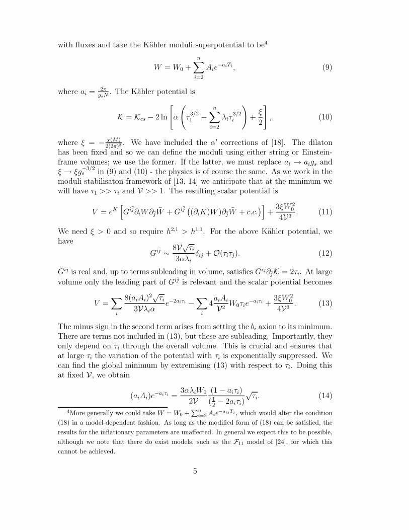
We illustrate the form of the resulting inflationary potential in figure 1, show-ing the inflaton and volume directions.
Figure 1: Inflationary potential: the inflaton lies along the x-direction and thevolume along the y-direction.
3 Inflationary Potential and Parameters
Let us now quantify the resulting potential and compute the inflationary param-eters. The inflationary potential is read off from (13) to be
Vinf = V0 −4τnW0anAne
−anτn
V2, (19)
as the double exponential in (13) is irrelevant during inflation. During inflationV0 is constant and can be parametrised as
V0 =βW 2
0
V3. (20)
7
( 1V3 is the scale of the potential during inflation). However, τn is not canonically
normalised, as to leading order in volume
Knn =3λ
8√
τnV. (21)
The canonically normalised field is
τ cn =
√
4λ
3V τ3
4
n . (22)
In terms of τ cn, the inflationary potential is
V = V0 −4W0anAn
V2
(
3V4λ
)2/3
(τ cn)4/3 exp
[
−an
(
3V4λ
)2/3
(τ cn)4/3
]
. (23)
This is similar, but not identical, to the textbook potential V = V0(1 − e−τ ).Although τ c
n is canonically normalised, it has no natural geometric interpretationand for clarity we shall express the inflationary parameters in terms of τn, thecycle volume.
The slow-roll parameters are defined by
ǫ =M2
P
2
(
V ′
V
)2
, (24)
η = M2P
V ′′
V, (25)
ξ = M4P
V ′V′′′
V 2, (26)
with the derivatives being with respect to τ cn. These can be evaluated to give
ǫ =32V3
3β2W 20
a2nA
2n
√τn(1 − anτn)2e−2anτn ,
η = − 4anAnV2
3λ√
τnβW0
[
(1 − 9anτn + 4(anτn)2)e−anτn]
, (27)
ξ =−32(anAn)2V4
9β2λ2W 20 τn
(1 − anτn)(1 + 11anτn − 30(anτn)2 + 8(anτn)2)e−2anτn .
Then ξ << ǫ, η << 1 provided that e−anτn << 1V2 .
Within the slow-roll approximation, the spectral index and its running aregiven by
n − 1 = 2η − 6ǫ + O(ξ), (28)
dn
d ln k= 16ǫη − 24ǫ2 − 2ξ. (29)
8
The number of efoldings is given by
Ne =
∫ φ
φend
V
V ′dφ, (30)
which may be expressed as
Ne =−3βW0λn
16V2anAn
∫ τn
τendn
eanτn
√τn(1 − anτn)
dτn. (31)
Matching the COBE normalisation for the density fluctuations δH = 1.92× 10⁻⁵
requiresV 3/2
M3P V ′
= 5.2 × 10⁻⁴, (32)
where the LHS is evaluated at horizon exit, Ne = 50 − 60 efoldings before theend of inflation. This condition can be expressed as
(
g4s
8π
)
3λβ3W 20
64√
τn(1 − anτn)2
(
W0
anAn
)2e2anτn
V6= 2.7 × 10⁻⁷. (33)
We have here included a factor of g4s
8πthat should properly be included as an overall
normalisation in V - see [14]. The condition (32) determines the normalisation ofthe potential and in practice we use it as a constraint on the stabilised volume.
Finally, the tensor-to-scalar ratio is
r ∼ 12.4ǫ. (34)
3.1 Footprint of the Model
We now want to determine the inflationary predictions for the above model. In theabove model there are various undetermined parameters arising from the detailedmicrophysics, such as the threshold correction A or tree-level superpotential W0.In principle, these are determined by the specific Calabi-Yau with its brane andflux configurations, but they can be prohibitively difficult to calculate in realisticexamples. However, it turns out that the most important results are independentof these parameters. In particular, solving equations (28) to (34) numerically, wefind the robust results
η ≈ − 1
Ne
, (35)
ǫ < 10−12, (36)
ξ ≈ − 2
N2e
. (37)
9
These results are not so surprising given the similarity of the potential to thetextbook form V0(1 − e−τ ). Taking a range of Ne = 50 → 60, we obtain in theslow-roll approximation
0.960 < n < 0.967, (38)
−0.0006 < dnd lnk
< −0.0008, (39)
0 < |r| < 10−10, (40)
where the uncertainties above arise principally from the number of e-foldings. Ifwe go beyond the slow-roll approximation, the expression for n will receive O(ξ)corrections - these are minimal and can be neglected.
To evaluate the inflationary energy scale, it is convenient to reformulate theCOBE normalisation of density perturbations δH = 1.92 × 10⁻⁵ as
V 1/4
ǫ1/4= 6.6 × 10¹⁶GeV. (41)
Unlike the predictions for the spectral index, the required internal volume isparameter-dependent. For typical values of the microscopic parameters this isfound numerically to take a range of values
105l6s ≤ V ≤ 107l6s , (42)
where ls = (2π)√
α′. As the moduli stabilisation mechanism of [13, 14] naturallygenerates exponentially large volumes, there is no difficulty in achieving thesevalues. The range of ǫ at horizon exit is 10−13 ≥ ǫ ≥ 10−15, and thus theinflationary energy scale is rather low,
Vinf ∼ 1013GeV. (43)
This implies in particular that tensor perturbations would be unobservable inthis model.
There is no practical upper limit on the number of efoldings attainable. Thisis large-field inflation and the potential is exponentially flat as the inflaton 4-cycleincreases in volume. A very large number of efoldings is achieved by a very smallvariation in the inflaton and barring cancellations we would expect Ne,total >> 60in these models.
In these compactifications, the lightest non-axionic modulus has a mass [14]
M ∼ MP
V3/2. (44)
Thus even at the larger end of volumes M >> O(10)TeV and there is no cos-mological moduli problem. As indicated earlier, there is also not a problem withinitial conditions for inflation. Given that the moduli attain their minimum, the
10
inflaton is simply the last Kahler modulus to roll down to the minimum. Wedo not need to worry about interference from the evolution of the other mod-uli. Once they roll down to the minimum they become heavy and will rapidlydecouple from inflationary dynamics.
We have nothing new to say on the cosmological overshoot problem. It isdifficult to see how progress may be achieved here without an adequate formula-tion of initial conditions for the universe. This problem is amplified by the factthat typical Calabi-Yaus have hundreds of both complex structure and Kahlermoduli; it is very difficult to give a well-motivated choice for the initial valuesand evolution of so many moduli. (For the possibility that damping can removethe overshoot problem see [26, 27, 28]).
3.2 Additional Corrections and Extensions
The inflationary mechanism presented here relies on the exponential flatness ofthe τn direction at constant volume. This is unbroken by the tree-level Kahlerpotential, the (α′)3 correction and the uplift term. Let us briefly discuss effectsthat might spoil this.
Let us first focus on superpotential effects. The nonrenormalisation theoremsguarantee that the Kahler moduli cannot appear perturbatively in W . However,the flatness could be spoiled if the gauge kinetic functions Ai depended poly-nomially on the Kahler moduli. A term A(Tj)e
−Ti in the superpotential wouldlead to an effective polynomial term for Tj once Ti was stabilised. However, theAi must be holomorphic in Ti and respect the axion shift symmetries, and sothis polynomial dependence on Ti cannot occur. Indeed, in models for whichthe threshold corrections have been computed explicitly, there is no dependenceof the gauge kinetic functions on the Kahler moduli [19]. Combined with non-renormalisation results, this means that the exponential flatness cannot be liftedby superpotential effects.
The other possibility is that the exponential flatness may be lifted by correc-tions to the Kahler potential that depend on τn. Considering first bulk terms,both the tree-level Kahler potential and the O(α′3) correction computed in [18]have the property that their contribution to the scalar potential is only a functionof the volume and has no explicit dependence on the moduli. These then do notaffect the constant volume flatness of the τn direction. It would be interesting,but difficult, to determine whether this feature extends beyond the terms so farcomputed.
There are also open string Kahler corrections such as those recently computedin [19]. Of necessity, this computation is restricted to certain toroidal orientifoldswith D3 and D7 branes. The 1-loop corrections determined there are subdomi-nant in the scalar potential to the O(α′3) corrections, although they give a largercontribution to the Kahler potential. This counterintuitive result is due to the
11
fact that a Kahler correction
K + δK = −2 ln(V) +ǫ
V2/3
only gives in the scalar potential
δV
V=
O(ǫ)
V4/3.
Thus O(V−2/3) corrections to the Kahler potential are in fact subdominant in thescalar potential to O(V−1) corrections. This result makes the volume stabilisationmechanism of [13, 14] more robust. For the models for which the string loopcomputation can be performed, there is no analogue of the τn blow-up field andso it is unclear whether and in what fashion these might appear in the 1-loopcorrection to the Kahler potential. There are however physical constraints: eK
appears in the scalar potential and so must behave sensibly in the limits of bothsmall and large τn.
There are also field theory loop corrections determined in [20]. These areagain subdominant in the scalar potential to the O(α′3) corrections used abovefor volume stabilisation. This computation again does not have an analogue ofthe blow-up modes we have used for the inflaton.
The upshot is that the exponential flatness of the τn direction is not broken byany of the known corrections. In general, any correction that can be expressedin terms of the overall volume will not alter the exponential flatness of the τn
direction. If corrections existed which did break this exponential flatness, itwould be necessary to examine their form and magnitude - it is not after allnecessary that the exponential flatness survive for all values of τn, but merely forthose relevant during the last sixty e-folds.
Finally, we have used an oversimplified form for the Calabi-Yau, picturingit as simply a combination of a volume cycle and blow-up modes. This is notnecessary for the inflationary mechanism described here. Whilst in (8) we as-sumed h1,1−1 moduli to be blow-ups whose only nonvanishing triple intersectionwas with themselves, a single such modulus would be perfectly adequate as aninflaton. Indeed, even this is not necessary - the minimal requirement is simplya flat direction, which originates from the no-scale behaviour and is broken bynonperturbative effects. The condition necessary to ensure the volume is stableduring inflaton will then be a generalisation of (18).
4 Discussion
We have presented a general but simple scenario of inflation in string theory thatdoes not require fine tuning of parameters, applies to a very large class of compact-ifications and is predictive at the level that can be ruled out within a few years.
12
This scenario realises large field inflation in a natural way. The main propertiesof these models are the existence of flat directions broken by non-perturbativeeffects. The flat directions have their origins in the no-scale property of theKahler potential and are generic for IIB Kahler moduli, as is the appearanceof instanton-generated nonperturbative superpotentials. The scenario is embed-ded in the exponentially large volume compactifications of [13, 14] and requiresh2,1 > h1,1 and h1,1 > 2. This last requirement is necessary to ensure that thevolume is stabilised during inflation.
Notice that the volumes required to obtain inflation, while large, are notextremely large as the string scale is only a few orders of magnitude below thePlanck scale. The necessary volumes of O(105 − 107) in string units can beobtained by natural choices of the exponential parameters ai (a ∼ 2π
3in the
simplest cases) [14].Although there are many moduli, the inflationary period reduces to a single-
field case. This is because the inflaton is simply the last modulus to roll down toits minimum, and once other moduli attain their minimum they rapidly becomeheavy and decouple from inflationary dynamics. In principle there are at leasttwo other fields that may have a nontrivial role during the cosmological evolution.One is the axion partner of the inflaton field. We have chosen this to sit at theminimum of its oscillatory potential, at least for the last sixty efolds. This is nota strong assumption - because the inflaton direction is so flat, there is a lot oftime for the axion to relax from a possibly non-zero inital value to its minimumbefore the last sixty efolds start. (Remember that depending on initial conditionsthe total number of efolds may be many orders of magnitude larger than 60.) Itwould nonetheless be interesting to study a multiple field inflation configurationin which both fields contribute to the density perturbations [29].
There is also a second direction which is extremely flat, corresponding tothe axionic partner of the overall volume modulus. This field is so light, withm << 10−300 GeV [14] both during and after inflation, that it will not play a rolein the cosmological evolution.
We have considered inflation as occurring at the top of a waterfall, and infla-tion ending as the moduli roll down to the waterfall. It may also be interestingto consider the case where there are multiple waterfalls. By appropriately tuningthe uplift we could arrange that the current vacuum energy corresponds to thetop of a waterfall rather than the bottom. As the field would be slowly rollingthis would then correspond to quintessence.
Another open question concerns reheating. Note that unlike brane inflation,in which reheating is driven by tachyon condensation [6] requiring non-trivialstring theory dynamics to be understood [30], in our case, as in racetrack in-flation, reheating is a pure field theory problem that only requires the study ofthe matter/inflaton couplings. In this respect, if the standard model lies on D7branes wrapping the four-cycle whose size is determined by the inflaton field, theinflaton can decay directly to the gauge fields of the standard model through the
13
coupling τnF µνFµν . This can give rise to efficient reheating as discussed in e.g.[31]. If the standard model lies elsewhere, the inflaton will couple to standardmodel fields through higher dimension operators and a more detailed analysis isrequired. (For a recent analysis of reheating in brane-antibrane inflation see [32]).
It is worth comparing aspects of this mechanism with other inflationary mod-els obtained from string theory. Besides the issue of fine tuning, it differs fromracetrack inflation and tachyon driven inflation in that it corresponds to large fieldrather than hill-top inflation. In principle our scenario is closer to brane separa-tion inflation, but we do not need a second field to end inflation and in particulardo not predict the existence of remnant cosmic strings from the reheating era.Numerically, our predictions are close to racetrack inflation although with thespectral index within a more comfortable range. The exponentially flat directionresembles the mechanism of [8], with the advantage that moduli stabilisation isnow derived and not assumed.
Let us finally discuss the generality of our scenario. The main technicalassumption we have used is the direct expression for the volume in terms ofthe Kahler moduli (8). This was overkill - the only part of the assumption weactually used was that the inflaton modulus appears alone in the volume asV = . . . − (Tn + Tn)
3
2 . As indicated above, we can relax even this: the abso-lute minimal requirement is simply the existence of a flat direction broken bynonperturbative effects. There may be several possible inflationary directions -in the above model, τ2, . . . , τn are all good candidates - with the particular onechosen determined by which Kahler modulus is last to attain its minimum. Ineach case we expect similar physics to emerge with a robust prediction on thespectral index of density perturbations. It is very exciting that such a simplestring scenario has the basic properties needed for a realisation of cosmologicalinflation with predictions that can be confirmed or ruled out in the near future.
Acknowledgements
We acknowledge useful conversations with P. Berglund, C. Burgess, S. Kachruand B. van Tent. The research of FQ is partially funded by PPARC and a RoyalSociety Wolfson merit award. JC is grateful to EPSRC for a research studentship.
References
[1] S. B. Giddings, S. Kachru and J. Polchinski, “Hierarchies fromfluxes in string compactifications,” Phys. Rev. D 66, 106006 (2002)[arXiv:hep-th/0105097].
14
[2] S. Kachru, R. Kallosh, A. Linde and S. P. Trivedi, “De Sitter vacua in stringtheory,” Phys. Rev. D 68, 046005 (2003) [arXiv:hep-th/0301240].
[3] C. L. Bennett et al., “First Year Wilkinson Microwave Anisotropy Probe(WMAP) Observations: Preliminary Maps and Basic Results,” Astrophys.J. Suppl. 148 (2003) 1 [arXiv:astro-ph/0302207].
[4] P. Binetruy and M. K. Gaillard, “Candidates For The Inflaton Field InSuperstring Models,” Phys. Rev. D 34 (1986) 3069; T. Banks, M. Berkooz,S. H. Shenker, G. W. Moore and P. J. Steinhardt, “Modular cosmology,”Phys. Rev. D 52 (1995) 3548 [arXiv:hep-th/9503114].
[5] G. R. Dvali and S. H. H. Tye, “Brane inflation,” Phys. Lett. B 450, 72(1999) [arXiv:hep-ph/9812483].
[6] C. P. Burgess, M. Majumdar, D. Nolte, F. Quevedo, G. Rajesh andR. J. Zhang, “The inflationary brane-antibrane universe,” JHEP 0107, 047(2001) [arXiv:hep-th/0105204].
[7] G. R. Dvali, Q. Shafi and S. Solganik, “D-brane inflation,”arXiv:hep-th/0105203.
[8] C. P. Burgess, P. Martineau, F. Quevedo, G. Rajesh and R. J. Zhang, “Braneantibrane inflation in orbifold and orientifold models,” JHEP 0203, 052(2002) [arXiv:hep-th/0111025].
[9] J. J. Blanco-Pillado et al., “Racetrack inflation,” JHEP 0411, 063 (2004)[arXiv:hep-th/0406230].
[10] S. Kachru, R. Kallosh, A. Linde, J. Maldacena, L. McAllister andS. P. Trivedi, “Towards inflation in string theory,” JCAP 0310 (2003) 013[arXiv:hep-th/0308055].
[11] J. P. Hsu, R. Kallosh and S. Prokushkin, “On brane inflation with volumestabilization,” JCAP 0312 (2003) 009 [arXiv:hep-th/0311077]; F. Koyama,Y. Tachikawa and T. Watari, “Supergravity analysis of hybrid inflationmodel from D3-D7 system”, [arXiv:hep-th/0311191]; H. Firouzjahi andS. H. H. Tye, “Closer towards inflation in string theory,” Phys. Lett. B584 (2004) 147 [arXiv:hep-th/0312020]. J. P. Hsu and R. Kallosh, “Volumestabilization and the origin of the inflaton shift symmetry in string theory,”JHEP 0404 (2004) 042 [arXiv:hep-th/0402047];
[12] C. P. Burgess, J. M. Cline, H. Stoica and F. Quevedo, “Inflation in re-alistic D-brane models,” [arXiv:hep-th/0403119]; J. M. Cline and H. Sto-ica, “Multibrane inflation and dynamical flattening of the inflaton po-tential,” arXiv:hep-th/0508029. O. DeWolfe, S. Kachru and H. Verlinde,
15
“The giant inflaton,” JHEP 0405 (2004) 017 [arXiv:hep-th/0403123].N. Iizuka and S. P. Trivedi, “An inflationary model in string theory,”arXiv:hep-th/0403203. K. Becker, M. Becker and A. Krause, “M-theoryinflation from multi M5-brane dynamics,” Nucl. Phys. B 715 (2005) 349[arXiv:hep-th/0501130]. D. Cremades, F. Quevedo and A. Sinha, “Warpedtachyonic inflation in type IIB flux compactifications and the open-stringcompleteness conjecture,” arXiv:hep-th/0505252. S. Dimopoulos, S. Kachru,J. McGreevy and J. G. Wacker, “N-flation,” arXiv:hep-th/0507205. E. Sil-verstein and D. Tong, “Scalar speed limits and cosmology: Accelerationfrom D-cceleration,” Phys. Rev. D 70 (2004) 103505 [arXiv:hep-th/0310221];M. Alishahiha, E. Silverstein and D. Tong, “DBI in the sky,” Phys. Rev.D 70 (2004) 123505 [arXiv:hep-th/0404084]; X. g. Chen, “Inflation fromwarped space,” arXiv:hep-th/0501184; H. Singh, “(A)symmetric tachyonrolling in de Sitter spacetime: A universe devoid of Planck density,”arXiv:hep-th/0508101.
[13] V. Balasubramanian, P. Berglund, J. P. Conlon and F. Quevedo, “System-atics of moduli stabilisation in Calabi-Yau flux compactifications,” JHEP0503 (2005) 007 [arXiv:hep-th/0502058].
[14] J. P. Conlon, F. Quevedo and K. Suruliz, “Large-volume flux compact-ifications: Moduli spectrum and D3/D7 soft supersymmetry breaking,”arXiv:hep-th/0505076.
[15] A. R. Liddle and D. H. Lyth, “Cosmological inflation and large-scale struc-ture,” CUP (2000).
[16] C. P. Burgess, R. Kallosh and F. Quevedo, “de Sitter string vacua fromsupersymmetric D-terms,” JHEP 0310, 056 (2003) [arXiv:hep-th/0309187].
[17] A. Saltman and E. Silverstein, JHEP 0411, 066 (2004)[arXiv:hep-th/0402135].
[18] K. Becker, M. Becker, M. Haack and J. Louis, “Supersymmetry breakingand alpha’-corrections to flux induced potentials,” JHEP 0206, 060 (2002)[arXiv:hep-th/0204254].
[19] M. Berg, M. Haack and B. Kors, “Loop corrections to volume mod-uli and inflation in string theory,” Phys. Rev. D 71, 026005 (2005)[arXiv:hep-th/0404087]. M. Berg, M. Haack and B. Kors, “String LoopCorrections to Kahler Potentials in Orientifolds,” arXiv:hep-th/0508043.M. Berg, M. Haack and B. Kors, “On Volume Stabilization by QuantumCorrections,” arXiv:hep-th/0508171.
[20] G. von Gersdorff and A. Hebecker, “Kaehler corrections for the volume mod-ulus of flux compactifications,” arXiv:hep-th/0507131.
16
[21] V. Balasubramanian and P. Berglund, “Stringy corrections to Kaehlerpotentials, SUSY breaking, and the cosmological constant problem,”JHEP 0411, 085 (2004) [arXiv:hep-th/0408054]. P. Berglund andP. Mayr, “Non-perturbative superpotentials in F-theory and string duality,”arXiv:hep-th/0504058.
[22] K. Bobkov, “Volume stabilization via alpha’ corrections in type IIB theorywith fluxes,” JHEP 0505, 010 (2005) [arXiv:hep-th/0412239]. A. Westphal,“Eternal inflation with alpha’ corrections,” arXiv:hep-th/0507079.
[23] P. Candelas and X. de la Ossa, “Moduli Space Of Calabi-Yau Manifolds,”Nucl. Phys. B 355, 455 (1991).
[24] F. Denef, M. R. Douglas and B. Florea, “Building a better racetrack,” JHEP0406, 034 (2004) [arXiv:hep-th/0404257].
[25] R. Brustein and P. J. Steinhardt, “Challenges for superstring cosmology,”Phys. Lett. B 302, 196 (1993) [arXiv:hep-th/9212049].
[26] N. Kaloper and K. A. Olive, “Dilatons in string cosmology,” Astropart. Phys.1 (1993) 185.
[27] N. Kaloper, J. Rahmfeld and L. Sorbo, “Moduli entrapment with primordialblack holes,” Phys. Lett. B 606, 234 (2005) [arXiv:hep-th/0409226].
[28] R. Brustein, S. P. de Alwis and P. Martens, “Cosmological stabiliza-tion of moduli with steep potentials,” Phys. Rev. D 70 (2004) 126012[arXiv:hep-th/0408160].
[29] B. van Tent, “Multiple-field inflation and the CMB,” Class. Quant. Grav.21 (2004) 349 [arXiv:astro-ph/0307048].
[30] G. Shiu, S. H. H. Tye and I. Wasserman, “Rolling tachyon in braneworld cosmology from superstring field theory,” Phys. Rev. D 67 (2003)083517 [arXiv:hep-th/0207119]; J. M. Cline, H. Firouzjahi and P. Mar-tineau, “Reheating from tachyon condensation,” JHEP 0211 (2002) 041[arXiv:hep-th/0207156]; N. Barnaby, C. P. Burgess and J. M. Cline,“Warped reheating in brane-antibrane inflation,” JCAP 0504 (2005) 007[arXiv:hep-th/0412040]; L. Kofman and P. Yi, “Reheating the universe af-ter string theory inflation,” arXiv:hep-th/0507257. A. R. Frey, A. Mazum-dar and R. Myers, “Stringy Effects During Inflation and Reheating,”arXiv:hep-th/0508139.
[31] A. D. Linde, “Particle Physics and Inflationary Cosmology,” Harwood (1990)362 p. (Contemporary concepts in physics, 5) arXiv:hep-th/0503203.
17
[32] D. Chialva, G. Shiu and B. Underwood, “Warped reheating in multi-throatbrane inflation,” arXiv:hep-th/0508229.
18


