NBER WORKING PAPER SERIES

DISAGREEMENT ABOUT INFLATION EXPECTATIONS

N. Gregory MankiwRicardo Reis

Justin Wolfers

Working Paper 9796http://www.nber.org/papers/w9796

NATIONAL BUREAU OF ECONOMIC RESEARCH1050 Massachusetts Avenue

Cambridge, MA 02138June 2003

We would like to thank Richard Curtin and Guhan Venkatu for help with data sources and Simon Gilchrist,Robert King and John Williams for their comments. Doug Geyser and Cameron Shelton provided researchassistance. Reis is grateful to the Fundacao Ciencia e Tecnologia, Praxis XXI, for financial support. Theviews expressed herein are those of the authors and not necessarily those of the National Bureau of EconomicResearch.

©2003 by N. Gregory Mankiw, Ricardo Reis, and Justin Wolfers. All rights reserved. Short sections of textnot to exceed two paragraphs, may be quoted without explicit permission provided that full credit including© notice, is given to the source.

Disagreement about Inflation ExpectationsN. Gregory Mankiw, Ricardo Reis, and Justin WolfersNBER Working Paper No. 9796June 2003JEL No. E3, D8, E0, E1

ABSTRACT

Analyzing 50 years of inflation expectations data from several sources, we document substantial

disagreement among both consumers and professional economists about expected future inflation.

Moreover, this disagreement shows substantial variation through time, moving with inflation, the

absolute value of the change in inflation, and relative price variability. We argue that a satisfactory

model of economic dynamics must speak to these important business cycle moments. Noting that

most macroeconomic models do not endogenously generate disagreement, we show that a simple

"sticky-information" model broadly matches many of these facts. Moreover, the sticky-information

model is consistent with other observed departures of inflation expectations from full rationality,

including autocorrelated forecast errors and insufficient sensitivity to recent macroeconomic news.

N. Gregory Mankiw Ricardo Reis Justin WolfersDepartment of Economics Department of Economics Graduate School of BusinessHarvard University Harvard University Stanford UniversityLittauer 223 Cambridge, MA 02138 518 Memorial WayCambridge, MA 02138 reis@fas.harvard.edu Stanford, CA 94305and NBER and NBERngmankiw@harvard.edu jwolfers@stanford.edu

1

I. INTRODUCTION

At least since Milton Friedman's renowned presidential address to the American

Economic Association in 1968, expected inflation has played a central role in the analysis

of monetary policy and the business cycle. How much expectations matter, whether they

are adaptive or rational, how quickly they respond to changes in the policy regime, and

many related issues have generated heated debate and numerous research studies. Yet

throughout this time, one obvious fact is routinely ignored: Not everyone has the same

expectation.

This oversight is probably explained by the fact that, in much standard theory,

there is no room for disagreement. In many (though not all) textbook macroeconomic

models, people share a common information set and form expectations conditional on

that information. That is, we often assume that everyone has the same expectation

because our models say they should.

The data easily rejects this assumption. Anyone who has looked at survey data on

expectations, either of the general public or of professional forecasters, can attest that

disagreement is substantial. For example, as of December 2002, the interquartile range of

inflation expectations for 2003 among economists goes from 1½ percent to 2½ percent.

Among the general public, the interquartile range of expected inflation goes from 0

percent to 5 percent.

This paper takes as its starting point the notion that this disagreement about

expectations is itself an interesting variable for students of monetary policy and the

business cycle. We document the extent of this disagreement and show that it varies over

2

time. More important, disagreement about expected inflation moves together with the

other aggregate variables that are more commonly of interest to economists. This fact

raises the possibility that disagreement may be a key to macroeconomic dynamics.

A recent macroeconomic model that has disagreement at its heart is the sticky-

information model proposed by Mankiw and Reis (2002). In this model, economic agents

update their expectations only periodically because of costs of collecting and processing

information. We investigate whether this model is capable of predicting the extent of

disagreement that we observe in the survey data, as well as its evolution over time.

The paper is organized as follows. Section II discusses the survey data on

expected inflation that will form the heart of this paper. Section III offers a brief and

selective summary of what is known from previous studies of survey measures of

expected inflation, replicating the main findings. Section IV presents an exploratory

analysis of the data on disagreement, documenting its empirical relationship to other

macroeconomic variables. Section V considers what economic theories of inflation and

the business cycle might say about the extent of disagreement. It formally tests the

predictions of one such theory—the “sticky information” model of Mankiw and Reis

(2002). Section VI compares theory and evidence from the Volcker disinflation. Section

VII concludes.

3

II. INFLATION EXPECTATIONS

Most macroeconomic models argue that inflation expectations are a crucial factor

in the inflation process. Yet the nature of these expectations—in the sense of precisely

stating whose expectations, over which prices, and over what horizon—is not always

discussed with precision. These are crucial issues for measurement.

The expectations of wage and price-setters are probably the most relevant. Yet it

is not clear just who these people are. As such, we analyze data from three sources. The

Michigan Survey of Consumer Attitudes and Behavior surveys a cross-section of the

population on their expectations over the next year. The Livingston Survey and the

Survey of Professional Forecasters (SPF) covers more sophisticated analysts –

economists working in industry and professional forecasters, respectively. Table 1

provides some basic detail about the structure of these three surveys.1

1 For further detail on the Michigan survey, the Livingston survey and the SPF, see Curtin (1996), Croushore (1997) and Croushore (1993), respectively.

4

Table 1: Surveys of Inflation Expectations Michigan Survey Livingston Survey Survey of

Professional Forecasters

Survey population

Cross-section of the general public.

Academic, business, finance, market and labor economists.

Market economists.

Survey Organization

Survey Research Center, University of Michigan.

Originally Joseph Livingston an economic journalist. Currently the Philadelphia Fed.

Originally ASA/NBER, currently the Philadelphia Fed.

Average number of respondents

Roughly 1000-3000 per quarter to 1977, then 500-700 per month to present.

48 per survey. (Varies from 14-63.)

34 per survey (Varies from 9-83.)

Starting date Qualitative questions: 1946 Q1. # Quantitative responses: January 1978.

1946, First half. (But the early data is unreliable.)#

GDP Deflator: 1968, Q4. CPI inflation: 1981, Q3.

Periodicity Most quarters from 1947 Q1 to 1977 Q4.

Every month from January 1978.

Semi-annual. Quarterly.

Inflation Expectation

Expected change in prices over the next 12 months.

Consumer Price Index (this quarter, in 2 quarters, in 4 quarters).

GDP deflator level Quarterly CPI levels (6 quarters).

Notes: # Our quantitative work will focus on the period from 1954 onward.

Although we have three sources of inflation expectations data, throughout this paper

we will focus on four, and occasionally five, series. Most papers analyzing the Michigan

data cover only the period since 1978 in which these data have been collected monthly

(on a relatively consistent basis), and respondents were asked to state their precise

quantitative inflation expectation. However, the Michigan Survey of Consumer Attitudes

and Behaviors has been conducted quarterly since 1946, even though for the first twenty

5

years respondents were asked only whether they expected prices to rise, fall, or stay the

same. We have put substantial effort into constructing a consistent quarterly time series

for the central tendency and dispersion of inflation expectations through time since 1948.

We construct these data by assuming that discrete responses to whether prices are

expected to rise, remain the same, or fall over the next year reflect underlying continuous

expectations drawn from a normal distribution, with a possibly time-varying mean and

standard deviation.2 We will refer to these constructed data as the “Michigan

experimental” series.

Our analysis of the Survey of Professional Forecasters will occasionally switch

between our preferred series, which is the longer time series of forecasts focusing on the

GDP deflator (starting in 1968, Q4), and the shorter CPI series (which only begins in

1981, Q3).

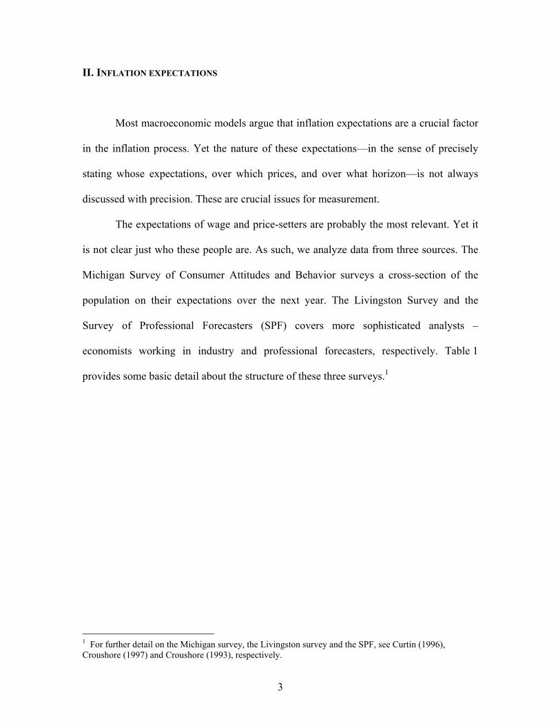
Figure 1 graphs our inflation expectations data (where the horizontal axis refers to

expectations at the endpoint of the relevant forecast horizon, rather than at the time the

forecast was made). Two striking features emerge from these plots. First, each series

yields relatively accurate inflation forecasts. And second, despite the different

populations being surveyed, they all tell a somewhat similar story.

2 Construction of this experimental series is detailed in the appendix, and we have published these data online at: www.stanford.edu/people/jwolfers.

6

Figure 1: Inflation Expectations and the Inflation Rate

0

5

10

15

0

5

10

15

1950 1960 1970 1980 1990 2000 1950 1960 1970 1980 1990 2000

Michigan Survey Michigan Experimental

Livingston SPF: GDP Deflator

Year-ended inflation rate Expected Inflation

Yea

r-en

ded

infl

atio

n ra

te, %

Actual and forecast shown at endpoint of horizon

Median Inflation Expectations and Actual Inflation

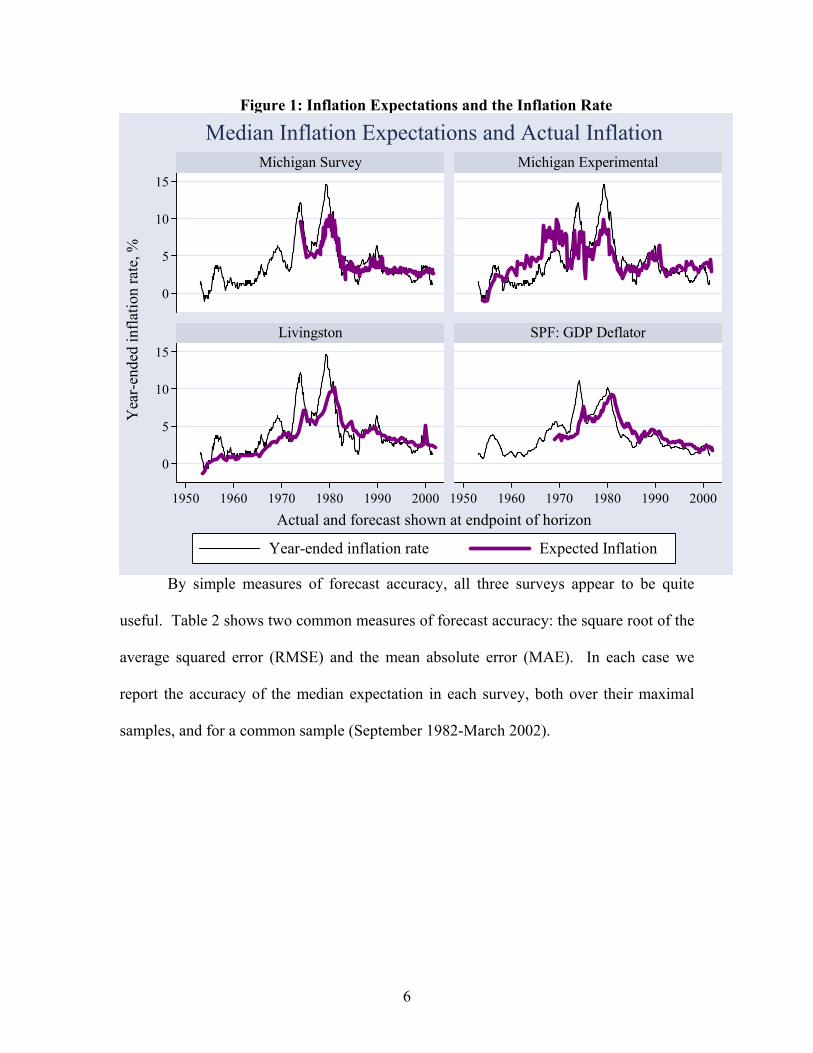
By simple measures of forecast accuracy, all three surveys appear to be quite

useful. Table 2 shows two common measures of forecast accuracy: the square root of the

average squared error (RMSE) and the mean absolute error (MAE). In each case we

report the accuracy of the median expectation in each survey, both over their maximal

samples, and for a common sample (September 1982-March 2002).

7

Table 2: Inflation Forecast Errors Michigan Michigan

ExperimentalLivingston SPF – GDP

Deflator SPF – CPI

Panel A: Maximal Sample Sample

Nov. 1974-May 2002

1954, Q4 –2002, Q1

1954, H1-2001, H2

1969, Q4 –2002, Q1

1982, Q3 -2002, Q1

RMSE 1.65% 2.32% 1.99% 1.62% 1.29% MAE 1.17% 1.77% 1.38% 1.22% 0.97%

Panel B: Common time period (September 1982—March 2002) RMSE 1.07% 1.24% 1.28% 1.10% 1.29% MAE 0.85% 0.95% 0.97% 0.91% 0.97%

Panel A suggests that inflation expectations are relatively accurate. Moreover, as

the group making the forecast becomes increasingly sophisticated, forecast accuracy

appears to improve. However, Panel B suggests that these differences across groups

largely reflect the different periods over which each survey has been conducted. For the

common sample that all five measures have been available, they are all approximately

equally accurate.

Of course, these results reflect the fact that these surveys have a similar central

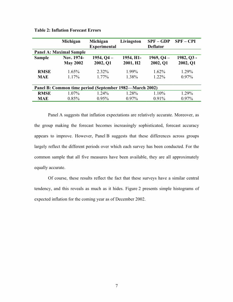
tendency, and this reveals as much as it hides. Figure 2 presents simple histograms of

expected inflation for the coming year as of December 2002.

8

Figure 2: Distribution of Inflation Expectations

0

10

20

30

Prop

ortio

n of

resp

onde

nts

-1 0 1 2 3Expected Inflat ion Over the Year to December 2 003, %

E mpirical Dist r ibut io n

K erne l De nsity Est im ate

Livingst on Survey and SPF, combined

Professional Economists

0

10

20

30

-5 - 2.5 0 2 .5 5 7.5 10Expected Inflat ion Over the Year to December 2003, %

Empirical Dist ribut ion

Kernel Density Est imate

Expectat ions < -5% a nd >10% tru ncated to en dpoin ts

M ichigan Survey

ConsumersDistribution of Inflation Expectations

Here the differences among these populations become starker. The left panel

pools responses from the two surveys of economists and shows some agreement on

expectations, with most respondents expecting inflation in the 1½-3 percent range. The

survey of consumers reveals substantially greater disagreement. The interquartile range

of consumer expectations stretches from 0 to 5 percent and this distribution shows quite

long tails, with 5 percent of the population expecting deflation, while 10 percent expect

inflation of at least 10 percent. These long tails are a feature throughout our sample, and

are not a particular reflection of present circumstances. Our judgment (following Curtin,

1996) is that these extreme observations are not particularly informative, and so we focus

on the median and interquartile range as the relevant indicators of central tendency and

disagreement, respectively.

9

The extent of disagreement within each of these surveys varies dramatically over

time. Figure 3 shows the interquartile range over time for each of our inflation

expectations series.

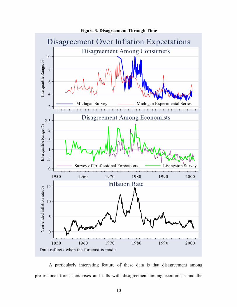
10

Figure 3. Disagreement Through Time

2

4

6

8

10

Inte

rqua

rtile

Ran

ge, %

Michigan Survey Michigan Experimental Series

Disagreement Among Consumers

0

.5

1

1.5

2

2.5

Inte

rqua

rtile

Ran

ge, %

1950 1960 1970 1980 1990 2000

Survey of Professional Forecasters Livingston Survey

Disagreement Among Economists

0

5

10

15

Yea

r-en

ded

infl

atio

n ra

te, %

1950 1960 1970 1980 1990 2000

Inflation Rate

Date reflects when the forecast is made

Disagreement Over Inflation Expectations

A particularly interesting feature of these data is that disagreement among

professional forecasters rises and falls with disagreement among economists and the

11

general public. Table 3 confirms that all of our series show substantial co-movement.

This table focuses on quarterly data—by averaging the monthly Michigan numbers, and

linearly interpolating the semi-annual Livingston numbers. The top panel shows

correlation coefficients among these quarterly estimates. The bottom panel shows

correlation coefficients across a smoothed version of the data (a 5-quarter centered

moving average of the interquartile range). While the high frequency data exhibit

reasonable correlation, this co-movement is particularly strong when focusing on lower

frequency movements. (The experimental Michigan data shows a somewhat weaker

correlation, particularly in the high frequency data. This probably reflects measurement

error, caused by the fact that these estimates rely heavily on the proportion of the sample

expecting price declines—a small and imprecisely estimated fraction of the population.)

12

Table 3: Disagreement Through Time – Correlation Across Surveys(a)

Michigan Michigan

ExperimentalLivingston SPF-GDP

deflator SPF-CPI

Panel A: Actual quarterly data Michigan

1.000

Michigan experimental

0.682 1.000

Livingston

0.809 0.391 1.000

SPF-GDP deflator

0.700 0.502 0.712 1.000

SPF-CPI

0.667 0.231 0.702 0.688 1.000

Panel B: 5 quarter centered moving averages Michigan

1.000

Michigan experimental

0.729 1.000

Livingston

0.869 0.813 1.000

SPF-GDP deflator

0.850 0.690 0.889 1.000

SPF-CPI 0.868 0.308 0.886 0.865 1.000 a) Underlying data are quarterly – created by taking averages of monthly Michigan data, and linearly interpolating half-yearly Livingston data.

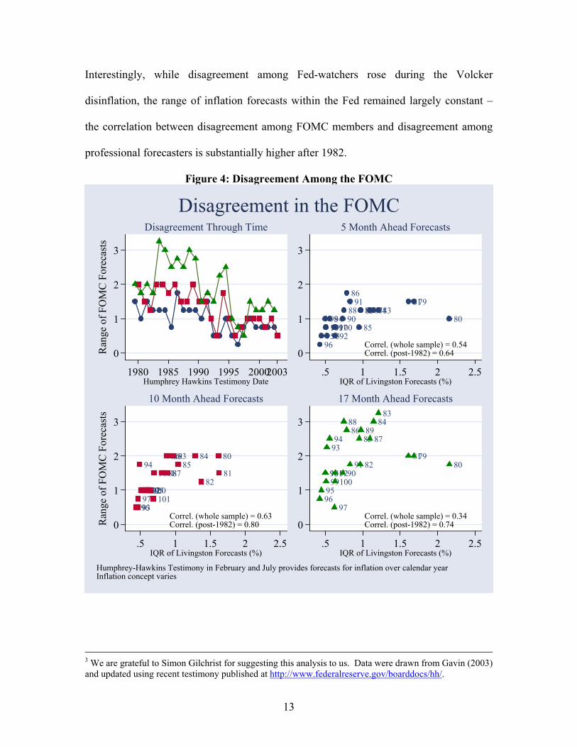
A final source of data on disagreement comes from the range of forecasts within

the FOMC, as published biannually since 1979 in Humphrey-Hawkins testimony.3

Unfortunately individual-level data are not released, so we simply look to describe the

broad pattern of disagreement among these experts. Figure 4 shows that there exists a

rough (and statistically significant) correspondence between disagreement among

policymakers and that among professional economists. The correlation of the range of

FOMC forecasts with the interquartile range of the Livingston population is either 0.34,

0.54 and 0.63, depending on which of the three available FOMC forecasts we use.

13

Interestingly, while disagreement among Fed-watchers rose during the Volcker

disinflation, the range of inflation forecasts within the Fed remained largely constant –

the correlation between disagreement among FOMC members and disagreement among

professional forecasters is substantially higher after 1982.

Figure 4: Disagreement Among the FOMC

0

1

2

3

Ran

ge o

f F

OM

C F

orec

asts

1980 1985 1990 1995 20002003Humphrey Hawkins Testimony Date

Disagreement Through Time

9695

981019993

949710092

9088

8691

85

82898784838179

80

0

1

2

3

.5 1 1.5 2 2.5IQR of Livingston Forecasts (%)

Correl. (whole sample) = 0.54Correl. (post-1982) = 0.64

5 Month Ahead Forecasts

969397

94

98102999210095101

909188

86

87

898385

84

82

80

81

0

1

2

3

Ran

ge o

f F

OM

C F

orec

asts

.5 1 1.5 2 2.5IQR of Livingston Forecasts (%)

Correl. (whole sample) = 0.63Correl. (post-1982) = 0.80

10 Month Ahead Forecasts

9695

9810199

9394

97

1009290

8886

91

85

82

8987

8483

817980

0

1

2

3

.5 1 1.5 2 2.5IQR of Livingston Forecasts (%)

Correl. (whole sample) = 0.34Correl. (post-1982) = 0.74

17 Month Ahead Forecasts

Humphrey-Hawkins Testimony in February and July provides forecasts for inflation over calendar yearInflation concept varies

Disagreement in the FOMC

3 We are grateful to Simon Gilchrist for suggesting this analysis to us. Data were drawn from Gavin (2003) and updated using recent testimony published at http://www.federalreserve.gov/boarddocs/hh/.

14

We believe that we have now established three important patterns in the data.

First, there is substantial disagreement within both naïve and expert populations about the

expected future path of inflation. Second, there are larger levels of disagreement between

consumers than that between experts. And third, even though professional forecasters,

economists and the general population show different degrees of disagreement, this

disagreement tends to exhibit similar time series patterns, albeit of a different amplitude.

One would therefore expect to find that the underlying causes behind this disagreement

are similar across all three datasets.

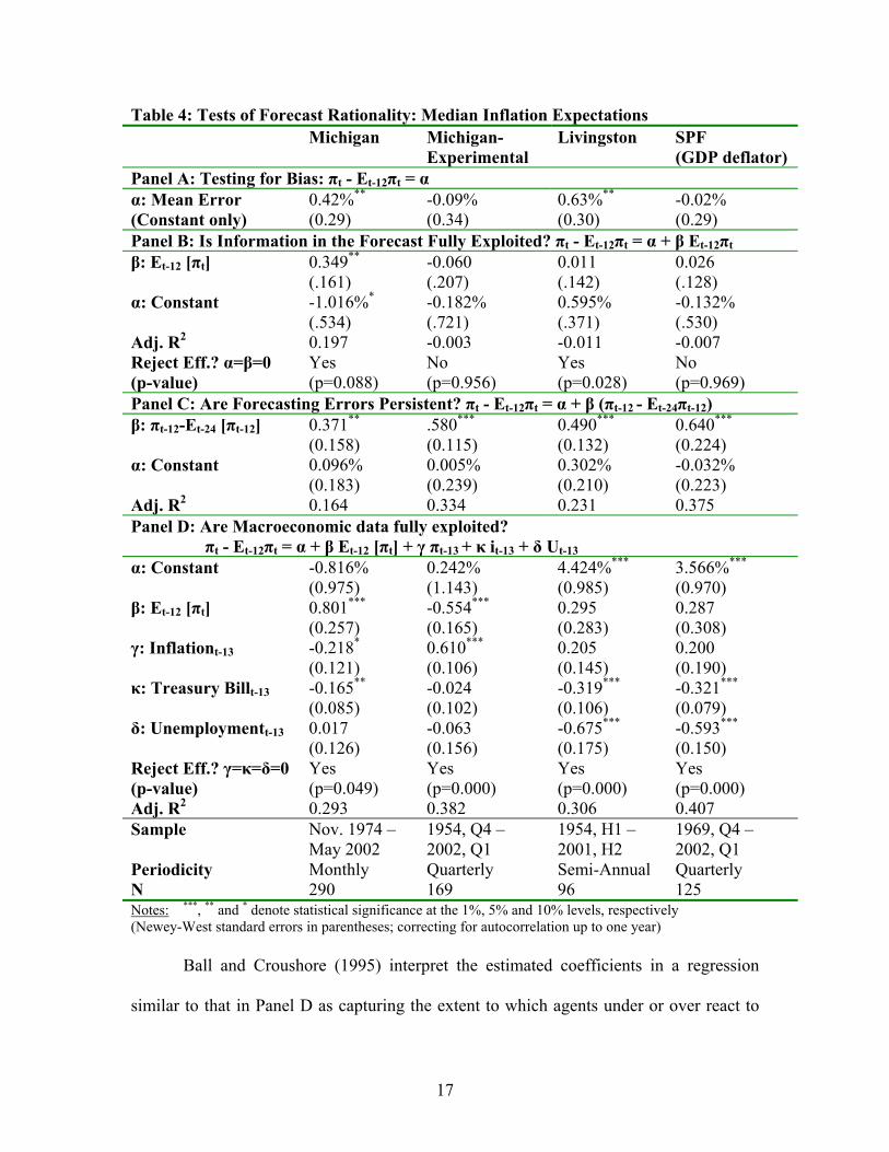
III. THE CENTRAL TENDENCY OF INFLATION EXPECTATIONS

Most studies analyzing inflation expectations data have explored whether

empirical estimates are consistent with rational expectations. The rational expectations

hypothesis has strong implications for the time series of expectations data, most of which

can be stated in terms of forecast efficiency. More specifically, rational expectations

implies (statistically) efficient forecasting, and efficient forecasts do not yield predictable

errors. We now turn to reviewing the tests of rationality commonly found in the

literature, and to providing complementary evidence based on the estimates of median

inflation expectations in our sample.4

The simplest test of efficiency is a test for bias: are inflation expectations centered

on the right value? Panel A of Table 4 reports these results, regressing expectation errors

on a constant. Median forecasts have tended to under-predict inflation in two of the four

4 Thomas (1999) provides a survey of this literature.

15

data series, and this divergence is statistically significant; that said, the magnitude of this

bias is small.5

Panel B tests whether there is information in these inflation forecasts themselves

that can be used to predict forecasting errors, by regressing the forecast error on a

constant and the median inflation expectation.6 Under the null of rationality, these

regressions should have no predictive power. Both the Michigan and Livingston series

can reject a rationality null on this score, while the other two series are consistent with

this (rather modest) requirement of rationality.

Panel C exploits a time-series implication of rationality, asking whether today’s

errors can be forecasted based on yesterday’s errors. In these tests, we regress this year’s

forecast error on the realized error over the previous year. Evidence of autocorrelation

suggests that there is information in last year’s forecast errors that is not being exploited

in generating this year’s forecast, violating the rationality null. We find robust evidence

of autocorrelated forecast errors in all surveys. When interpreting these coefficients, note

that they reflect the extent to which errors made a year ago persist in today’s forecast.

We find that on average around half of the error remains in the median forecast. One

might object that last year’s forecast error may not yet be fully revealed by the time this

year’s forecast is made, because inflation data are only published with one month lag.

Experimenting with slightly longer lags does not change these results significantly.7

5 Note that the construction of the Michigan experimental data makes the finding of bias unlikely for that series. 6 Some readers may be more used to seeing regressions of the form: πt= a+bEt-12πt, where the test for rationality is a joint test of a=0 and b=1. To see that our tests are equivalent, simply rewrite πt-Et-12πt=a+(1-b)Et-12πt and it can be seen that a test of a=0 and b=1 translates into a test that the constant and slope coefficient in this equation are both zero. 7 Interestingly, repeating this analysis with mean rather than median expectations yields weaker results.

16

Finally, Panel D asks whether inflation expectations take sufficient account of

publicly available information. We regress forecast errors on recent macroeconomic

data. Specifically, we analyze the inflation rate, the Treasury bill rate, and the

unemployment rate measured one month prior to the forecast, because these data are

likely to be the most recent published data when forecasts were made. We also control

for the forecast itself, thereby nesting the specification in Panel B. One might object that

using real-time data would better reflect the information available when forecasts were

made; we chose these three indicators precisely because they are subject to only minor

revisions. Across the three different pieces of macroeconomic information and all four

surveys, we often find statistical evidence that agents are not fully incorporating this

information in their inflation expectations. Simple bivariate regressions (not shown) yield

a qualitatively similar pattern of responses. The advantage of the multivariate regression

is that we can perform an F-test of the joint significance of the lagged inflation, interest

rates and unemployment rates in predicting forecast errors. In each case the

macroeconomic data are overwhelmingly jointly statistically significant, suggesting that

median inflation expectations do not adequately take account of recent available

information. Note that these findings do not depend on whether we condition on the

forecast of inflation.

17

Table 4: Tests of Forecast Rationality: Median Inflation Expectations Michigan Michigan-

Experimental Livingston SPF

(GDP deflator) Panel A: Testing for Bias: πt - Et-12πt = α α: Mean Error (Constant only)

0.42%**

(0.29) -0.09% (0.34)

0.63%** (0.30)

-0.02% (0.29)

Panel B: Is Information in the Forecast Fully Exploited? πt - Et-12πt = α + β Et-12πt β: Et-12 [πt] 0.349**

(.161) -0.060 (.207)

0.011 (.142)

0.026 (.128)

α: Constant -1.016%* (.534)

-0.182% (.721)

0.595% (.371)

-0.132% (.530)

Adj. R2 0.197 -0.003 -0.011 -0.007 Reject Eff.? α=β=0 (p-value)

Yes (p=0.088)

No (p=0.956)

Yes (p=0.028)

No (p=0.969)

Panel C: Are Forecasting Errors Persistent? πt - Et-12πt = α + β (πt-12 - Et-24πt-12) β: πt-12-Et-24 [πt-12] 0.371**

(0.158) .580*** (0.115)

0.490*** (0.132)

0.640*** (0.224)

α: Constant 0.096% (0.183)

0.005% (0.239)

0.302% (0.210)

-0.032% (0.223)

Adj. R2 0.164 0.334 0.231 0.375 Panel D: Are Macroeconomic data fully exploited? πt - Et-12πt = α + β Et-12 [πt] + γ πt-13 + κ it-13 + δ Ut-13 α: Constant -0.816%

(0.975) 0.242%

(1.143) 4.424%*** (0.985)

3.566%*** (0.970)

β: Et-12 [πt] 0.801*** (0.257)

-0.554*** (0.165)

0.295 (0.283)

0.287 (0.308)

γ: Inflationt-13 -0.218* (0.121)

0.610*** (0.106)

0.205 (0.145)

0.200 (0.190)

κ: Treasury Billt-13 -0.165** (0.085)

-0.024 (0.102)

-0.319*** (0.106)

-0.321*** (0.079)

δ: Unemploymentt-13 0.017 (0.126)

-0.063 (0.156)

-0.675*** (0.175)

-0.593*** (0.150)

Reject Eff.? γ=κ=δ=0 (p-value)

Yes (p=0.049)

Yes (p=0.000)

Yes (p=0.000)

Yes (p=0.000)

Adj. R2 0.293 0.382 0.306 0.407 Sample Nov. 1974 –

May 2002 1954, Q4 – 2002, Q1

1954, H1 – 2001, H2

1969, Q4 – 2002, Q1

Periodicity Monthly Quarterly Semi-Annual Quarterly N 290 169 96 125 Notes: ***, ** and * denote statistical significance at the 1%, 5% and 10% levels, respectively (Newey-West standard errors in parentheses; correcting for autocorrelation up to one year)

Ball and Croushore (1995) interpret the estimated coefficients in a regression

similar to that in Panel D as capturing the extent to which agents under or over react to

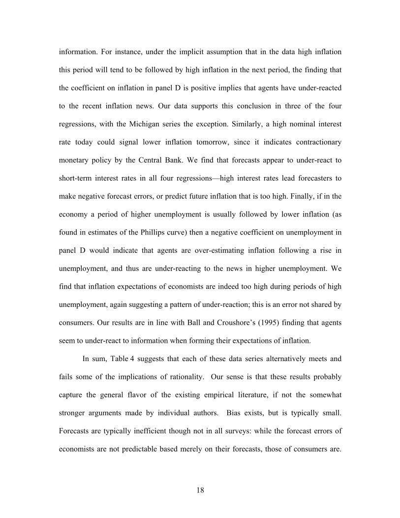
18

information. For instance, under the implicit assumption that in the data high inflation

this period will tend to be followed by high inflation in the next period, the finding that

the coefficient on inflation in panel D is positive implies that agents have under-reacted

to the recent inflation news. Our data supports this conclusion in three of the four

regressions, with the Michigan series the exception. Similarly, a high nominal interest

rate today could signal lower inflation tomorrow, since it indicates contractionary

monetary policy by the Central Bank. We find that forecasts appear to under-react to

short-term interest rates in all four regressions—high interest rates lead forecasters to

make negative forecast errors, or predict future inflation that is too high. Finally, if in the

economy a period of higher unemployment is usually followed by lower inflation (as

found in estimates of the Phillips curve) then a negative coefficient on unemployment in

panel D would indicate that agents are over-estimating inflation following a rise in

unemployment, and thus are under-reacting to the news in higher unemployment. We

find that inflation expectations of economists are indeed too high during periods of high

unemployment, again suggesting a pattern of under-reaction; this is an error not shared by

consumers. Our results are in line with Ball and Croushore’s (1995) finding that agents

seem to under-react to information when forming their expectations of inflation.

In sum, Table 4 suggests that each of these data series alternatively meets and

fails some of the implications of rationality. Our sense is that these results probably

capture the general flavor of the existing empirical literature, if not the somewhat

stronger arguments made by individual authors. Bias exists, but is typically small.

Forecasts are typically inefficient though not in all surveys: while the forecast errors of

economists are not predictable based merely on their forecasts, those of consumers are.

19

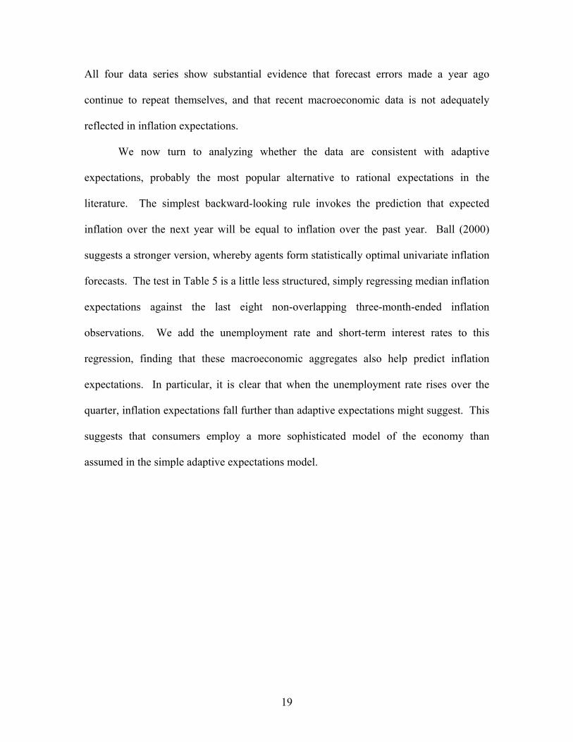
All four data series show substantial evidence that forecast errors made a year ago

continue to repeat themselves, and that recent macroeconomic data is not adequately

reflected in inflation expectations.

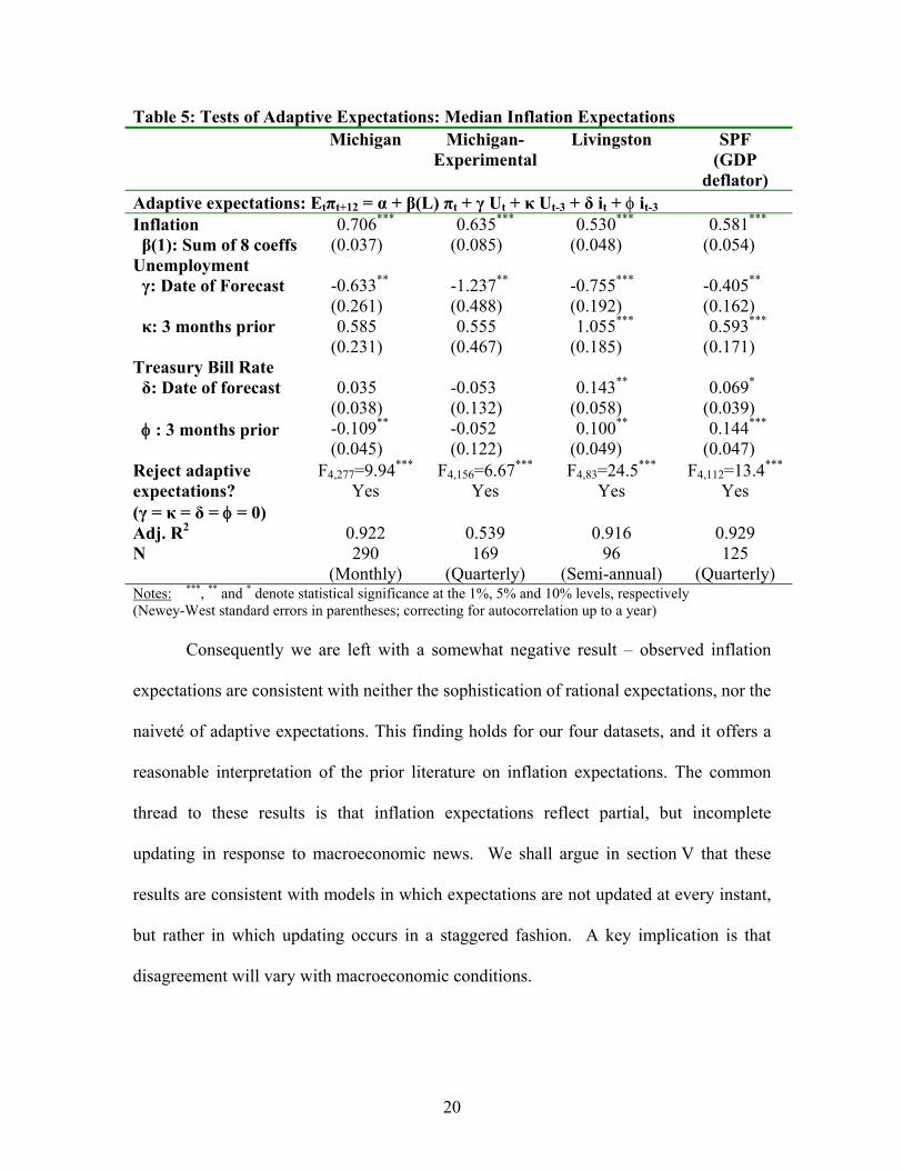
We now turn to analyzing whether the data are consistent with adaptive

expectations, probably the most popular alternative to rational expectations in the

literature. The simplest backward-looking rule invokes the prediction that expected

inflation over the next year will be equal to inflation over the past year. Ball (2000)

suggests a stronger version, whereby agents form statistically optimal univariate inflation

forecasts. The test in Table 5 is a little less structured, simply regressing median inflation

expectations against the last eight non-overlapping three-month-ended inflation

observations. We add the unemployment rate and short-term interest rates to this

regression, finding that these macroeconomic aggregates also help predict inflation

expectations. In particular, it is clear that when the unemployment rate rises over the

quarter, inflation expectations fall further than adaptive expectations might suggest. This

suggests that consumers employ a more sophisticated model of the economy than

assumed in the simple adaptive expectations model.

20

Table 5: Tests of Adaptive Expectations: Median Inflation Expectations Michigan Michigan-

ExperimentalLivingston SPF

(GDP deflator)

Adaptive expectations: Etπt+12 = α + β(L) πt + γ Ut + κ Ut-3 + δ it + φ it-3 Inflation β(1): Sum of 8 coeffs

0.706*** (0.037)

0.635*** (0.085)

0.530*** (0.048)

0.581*** (0.054)

Unemployment γ: Date of Forecast -0.633**

(0.261) -1.237** (0.488)

-0.755*** (0.192)

-0.405** (0.162)

κ: 3 months prior

0.585 (0.231)

0.555 (0.467)

1.055*** (0.185)

0.593*** (0.171)

Treasury Bill Rate δ: Date of forecast

0.035 (0.038)

-0.053 (0.132)

0.143** (0.058)

0.069* (0.039)

φ : 3 months prior

-0.109** (0.045)

-0.052 (0.122)

0.100** (0.049)

0.144*** (0.047)

Reject adaptive expectations? (γ = κ = δ = φ = 0)

F4,277=9.94*** Yes

F4,156=6.67***

Yes F4,83=24.5***

Yes F4,112=13.4***

Yes

Adj. R2 0.922 0.539 0.916 0.929 N 290

(Monthly) 169

(Quarterly) 96

(Semi-annual) 125

(Quarterly) Notes: ***, ** and * denote statistical significance at the 1%, 5% and 10% levels, respectively (Newey-West standard errors in parentheses; correcting for autocorrelation up to a year)

Consequently we are left with a somewhat negative result – observed inflation

expectations are consistent with neither the sophistication of rational expectations, nor the

naiveté of adaptive expectations. This finding holds for our four datasets, and it offers a

reasonable interpretation of the prior literature on inflation expectations. The common

thread to these results is that inflation expectations reflect partial, but incomplete

updating in response to macroeconomic news. We shall argue in section V that these

results are consistent with models in which expectations are not updated at every instant,

but rather in which updating occurs in a staggered fashion. A key implication is that

disagreement will vary with macroeconomic conditions.

21

IV. DISPERSION IN SURVEY MEASURES OF INFLATION EXPECTATIONS

Few papers have explored the features of the cross-sectional variation in inflation

expectations.

Bryan and Venkatu (2001) examine a survey of inflation expectations in Ohio

from 1998-2001, finding that women, singles, non-whites, high school dropouts and

lower income groups tend to have higher inflation expectations than other demographic

groups. They note that these differences are too large to be explained by differences in

the consumption basket across groups, but present suggestive evidence that differences in

expected inflation reflect differences in perceptions of current inflation rates. Vissing-

Jorgenson (this volume) also explores differences in inflation expectations across age

groups.

Souleles (2001) finds complementary evidence from the Michigan survey that

expectations vary by demographic group, a fact that he interprets as evidence of non-

rational expectations. Divergent expectations across groups lead to different expectation

errors, which he relates to differential changes in consumption across groups.

A somewhat larger literature has employed data on the dispersion in inflation

expectations as a rough proxy for “inflation uncertainty.” These papers have suggested

that highly dispersed inflation expectations are positively correlated with the inflation

rate, and conditional on current inflation, are related positively to the recent variance of

measured inflation (Cukierman and Wachtel 1979), to weakness in the real economy

(Mullineaux, 1980, Makin 1982), and alternatively to lower interest rates (Levi and

Makin, 1979, Bomberger and Frazer, 1981, and Makin 1983) and to higher interest rates

(Barnea, Dotan and Lakonishok, 1979, Brenner and Landskroner, 1983.) These

22

relationships do not appear to be particularly robust, and in no case is more than one set

of expectations data brought to bear on the question.

Our approach is consistent with a more literal interpretation of the second moment

of the expectations data: we interpret different inflation expectations as reflecting

disagreement in the population. That is, different forecasts reflect different expectations.

Llambros and Zarnowitz (1987) argue that disagreement and uncertainty are

conceptually distinct, and they make an attempt at unlocking the two empirically. Their

data on uncertainty derives from the SPF, which asks respondents to supplement their

point estimates with estimates of the probability that GDP and the implicit price deflator

will fall into various ranges. These two authors find only weak evidence that uncertainty

and disagreement share a common time series pattern. Intrapersonal variation in expected

inflation (“uncertainty”) is larger than interpersonal variation (“disagreement”), and while

there are pronounced changes through time in disagreement, uncertainty varies very little.

The most closely related approach to the macroeconomics of disagreement comes

from Carroll (2003b), who analyzes the evolution of the standard deviation of inflation

expectations in the Michigan Survey. Carroll provides an epidemiological model of

inflation expectations in which “expert opinion” slowly spreads person-to-person much

as disease spreads through a population. His formal model yields something very close

to the Mankiw and Reis (2002) formulation of the sticky-information model. In an agent-

based simulation, he proxies expert opinion by the average forecast in the Survey of

Professional Forecasters, and finds that his agent-based model tracks the time series of

disagreement quite well, although it cannot match the level of disagreement in the

population.

23

We now turn to analyzing the evolution of disagreement in greater detail.

Figure 3 showed the inflation rate and our measures of disagreement. That figure

suggested a relatively strong relationship between inflation and disagreement. A clearer

sense of this relationship can be seen in Figure 5.

Figure 5. Inflation and Disagreement

868687989898989898

868686

98989899988686

989897998 68 6

99978 79 9979999

86

979797979999

9497

83

9497

94

8383

94949595999994949594959994

92

99949611

09593

83

93

83

9397959693

96

92

96969596938796939195959 69494

929 119 293

96

929392

9 79 79 596

91

0

92

95

92950

9392

83

929 28 6

0

93859 38 5

196

93192

0

850

96

91

83

00

85

83

85

0

85185

8583

0

85

18587870

83

1087

83

858591

82

8887888886

8888

8 3

84

8 8

88888 4

88888 8

8 4

87

84

87

84848 484

87

84

879 0

9 1

8 889

82

8987

84

898989898990

849190

91

90

91

89

84

82

82

89

91

76

8989909 0908 9

9191

9076

82

77

90

9078

90

7678

907 8

8 2

82

777 777

78

82

8278

82

78

82

7 878

73

82

7878

8 1

787879

81818179

8 1

79817981

79818181

797 5

81

79

81

79797 9

80

798080

80808079

8080

80808080

2 .5

5

7.5

10

Consumers - Michigan

555455546161595 3

63

8665

646462626262

61

609859

986598639897

6058868699

565 66 59 98 69797

67

83

67

9495

66

9599

194569499839397

67

9593968796

5 8

6672

9492

9119 29 39 692939 5

7 2

9 285

157

7157

67

0969172

72083850087838585

66

82888884

7 18868

87848487

71

8889

71

68

8990916891

73

89

84

82

76

8990

6 9

69

76

7070

6969

7673

70

76

7 0

90

90

7 8

7 77 777

77

82

75

82

73

78

75

7 8

81

73787 5

81

747 975

81

74

81

797974

74

808079

8080

Consumers - Michigan Experimental

5554

54

5561615 9

5 3

53

86

64

646362626059

198

639897605 8

8 6566 5659 997

83

9495

6694

56

99

67

9396

58

72

929 193929 56 61

5771

57

670

96

7285

0

8783

858288

846 88487

71

8 8899091687689

69

70697673

70

90

77

77

75

8278

8 1

7378

7581

74

79 7480

79

80

1 .0

2 .0

3 .0

-5 0 5 10 15

Economists - Livingston

86

982981

98

9897

8 68 6

9999

86

9797

83

949595

991949499

83

93979593

96

8 79 67294929 119293

969293957292

85

171

0

96917272

0

8385008783858582888 88471

8887

8484

87

71

88

8971

899091689173

89848276

89

9 0

76

707069767370

769 090787777

7777827582

737 875

78

81737875

81

74

7 9

7581748179

79

74

8 080

79

80

80

-5 0 5 10 15

Economists - SPF

Inte

rqua

rtile

Ran

ge o

f Exp

ecte

d F

utur

e In

flat

ion(

%)

Inflation Over the Past Year(%)

Disagreement and Inflation

Beyond this simple relationship in levels, an equally apparent fact from Figure 3

is that when the inflation rate moves around a lot, dispersion appears to rise. This fact is

illustrated in Figure 6.

24

Figure 6. Changes in Inflation and Disagreement

9591

8 0

91

96

929694889 9

9 1

959595

78

96

931

94

888899899789

84

1

88889796899990958999

78

899995

939286

91

9699189

77

95

84

8 0

9384

909996

918 70

8 99 0

78

95009599960

80

84

77

890188

84

099890

80

89

78

99

90

0999989

75

84

78

89

8 4

0

84

84

90

0

9078

77

80

90

0

9084

84

0

8 4

8 78788

78

87

78

87

7879

8 7

7 8

87

88

87

79

87

8 0

87

7 97979

7979

79

80

79

797 9

80

7980

80

80

73

82

8 2

828276

82

8 3

8181

83

81

82

8383

81

828282

91

82

83

8 3

8 1

8 39191

81

9276

82

91

8 1

83

8786

82

92

8181

7683

86

83

81

81

928 69 18686

81

8686979286869292

98

869 89897

83

879285858585

9897

85

859490

80

18594

9 89 497

8 58 59 492

97

1

9 8858 51

9 89897979893

97

94

90198

7891

95

9186

9892

9793949093

96

9695

88

85

9093939694

77

88

9393949 69 49 48888

9 69 795

7 883

989 39 392

2 .5

5

7.5

10 Consumers - Michigan

91

9688

95

72

94

67

88

89

67

89846563

64

75

99

90

77

9 996

70

9 5

66

65

57

6262

870

7778

55

70

96

8077

0889 9

60

8 9

9 9

69

89

6969

84

69

73

6868

57

56

84

66

90

77

90

084087

68

78

66

5 6

7 8

8756

73

87

74

8079

79

79

7 3

798074

74

7473

828 2

75

83

81767581

8 2

81

8 3

9 1

76

9186

8 2

76

71

83

59

76

86

81

97

92

75

71

8692

71

715886

72

98

67

5455

85

61

85

721

80

72

989754161

85989794

90

1

58

95

91

92

67

59

94

63

70

8593969 4939 3

88

9 795

78

83

70

98

60

61

626264

6593

92

53

Consumers - Michigan Experimental

918872678889

6784

63

99

7 0

95

6 66 56 5

5 7

626207 7

78

5 5

9699606989

6 6

6 9

6 86 8

57

90

77

0

848 756

78

56

73

87

74

8 0

79

79

74 73

82

75

8 3

81 8 1

91

768682715976

8619792

75715872

53

545561

805 4

6185

9 89794901

5859

64

7085

96

94

9395

83

98

6 06 36 4

9 392

53

1 .0

2 .0

3 .0

-5 0 5

Economists - Livingston

919688957294

88898984

75

9990

77

99

9 6

709 5

87

0

7778

96

80

77

0

88

9 9

8 9

9 9

6989

84

73688490

779 00

84

087

78

78

8773

87

74

80

79

7979

7 3

79

80

747 473

8282

7583

817675

81

828183

917 6

91

8 6827671

837 68 6

181

9792

75

71

86

92

71

71

28 672

98

858572

1

80

72989 71

85

98

9794

9019591

9294708593

9 69 49393889 7957 8837098

93

92

-5 0 5

Economists - SPF

Inte

rqua

rtile

Ran

ge o

f Exp

ecte

d F

utur

e In

flat

ion(

%)

Inflation (Year to t) - Inflation(Year to t-12), %

Disagreement and the Change in Inflation

In all four datasets, large changes in inflation (in either direction) are correlated

with an increase in disagreement. This fanning out of inflation expectations following a

change in inflation is consistent with a process of staggered adjustment of expectations.

Of course, the change in inflation is (mechanically) related to its level, and we will

provide a more careful attempt at sorting out change and level effects below.

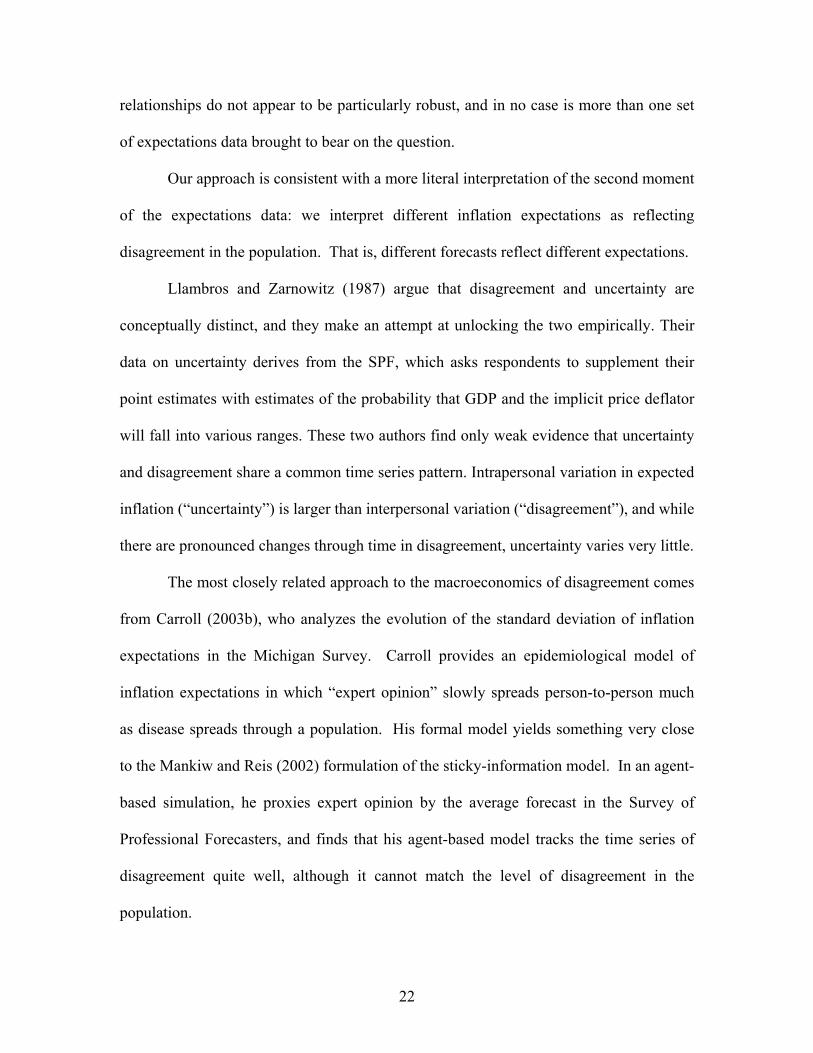
Figure 7 maps the evolution of disagreement and the real economy through time.

The chart shows our standard measures of disagreement, plus two measures of excess

capacity: an output gap constructed as the difference between the natural logs of actual

chain-weighted real output and trend output (constructed from a Hodrick-Prescott filter),

25

and shaded regions representing periods of economic expansion and contraction as

marked by the NBER Business Cycle Dating Committee.8

Figure 7: Disagreement and the Real Economy

The series on disagreement among consumers appears to rise during recessions, at

least through the second half of the sample. A much weaker relationship is observed

through the first half of the sample. Disagreement among economists shows a less

obvious relationship with the state of the real economy.

The final set of data that we examine can be thought of as either a cause or

consequence of disagreement in inflation expectations. We consider the dispersion in

8 We have also experimented using the unemployment rate as a measure of real activity, and obtained similar results.

26

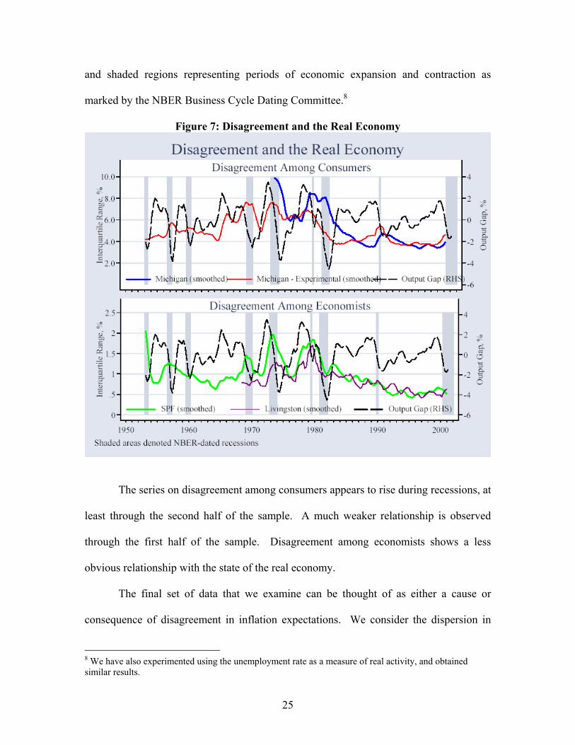
actual price changes across different CPI categories. That is, just as Bryan and Cecchetti

(1994) produce a weighted median CPI by calculating rates of inflation across 36

commodity groups, we construct a weighted interquartile range of year-ended inflation

rates across commodity groups. One could consider this a measure of the extent to which

relative prices are changing. We analyze data for the period December 1967-December

1997 provided by the Cleveland Fed. Figure 8 shows the median inflation rate, as well as

the 25th and 75th percentiles of the distribution of nominal price changes.

Figure 8: Distribution of Price Changes Across CPI Components

0

5

10

15

20

Infl

atio

n R

ate

/ IQ

R, %

-poi

nts

1970 1980 1990 2000

25th percentile inflation rate

75th percentile inflation rate

IQR of weighted component-level inflation rates over past year

Weighted percentiles, based on 36 CPI component indicesDistribution of Inflation Rates Across CPI Components

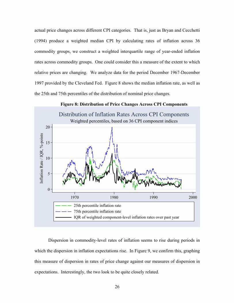
Dispersion in commodity-level rates of inflation seems to rise during periods in

which the dispersion in inflation expectations rise. In Figure 9, we confirm this, graphing

this measure of dispersion in rates of price change against our measures of dispersion in

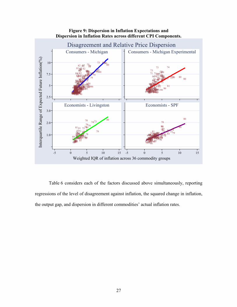
expectations. Interestingly, the two look to be quite closely related.

27

Figure 9: Dispersion in Inflation Expectations and Dispersion in Inflation Rates across different CPI Components.

9797969696979788

93

97969696899789

9293979593

92

96

92

9197

929391

969693929293959391919293949295948994969596

9193959597

929392

8895939491

979587

9192

898794959793

91

89909494908787

91

89

92

83

81

919595849687879494

84

91

90

9094878790

84

888988

91

9594

81

87

85

81

89

84

89

83

77

90

82

888585

88

8490

94

84

898887

84

81

84

8889

9085

90

82

88

84

878490

81

90

82

8483

82

76

83

83

898588

84

82

889787888676

828281

90

85

83

85

8383

86

7781

8586

8383

8685788685

82

83

777877

78

83

82

82

78

8586

78

82

86

76

86

82

79

8181

79

86

81

8578

78

8080

78

7980

78

79788079

75

78

79

86

79

78

79

86

81

79

79

80

86

8179

807980

73

80

80808080

2.5

5

7.5

10

Consumers - Michigan

9796978896899296979293

9196919389

949395959292

9593

91

94

7281

958787

90

9487

687190

71

8988

73

91838584948884

81

71

90

6768

908172

82

84

68

73

83897284

77

97

75

878882

71

76

76

85

72

86858385

73

69

76

86

76

77

82

777775

83

69

78

69

82

70

74707970

86

78788075

78

697074807979

86

75

74

81

737479 8080

Consumers - Michigan Experimental

9788

969692919393959294

72

81

9594

876890

718991

8384

88

84719067

81

68

73

8997

8776857286856976778277

75

8369

8270

74

70

86

78

78

8075

79

7473

79

80

1.0

2.0

3.0

-5 0 5 10 15

Economists - Livingston

9796978896

8992

96979293919691

9389

9493959592929593

91

9472

819587

87

9094877190

71

89887391838584

94

8884

81

71909081

72828468738389728477

97

75

87888271767685728685

8385

736976867677

827777

7583

788270

7470797086

78

78

8075

78

8079

7986

757481

737479

80

80

-5 0 5 10 15

Economists - SPF

Inte

rqua

rtil

e R

ange

of

Exp

ecte

d F

utur

e In

flat

ion(

%)

Weighted IQR of inflation across 36 commodity groups

Disagreement and Relative Price Dispersion

Table 6 considers each of the factors discussed above simultaneously, reporting

regressions of the level of disagreement against inflation, the squared change in inflation,

the output gap, and dispersion in different commodities’ actual inflation rates.

28

Table 6: Disagreement and the Business Cycle - Establishing Stylized Facts Michigan Michigan -

ExperimentalLivingston SPF

(GDP deflator)

Panel A: Bivariate Regressions (Each Cell Represents a Separate Regression) Inflation Rate 0.441***

(0.028) 0.228*** (0.036)

0.083*** (0.016)

0.092*** (0.013)

∆Inflation-squared 18.227*** (2.920)

1.259** (0.616)

2.682*** (0.429)

2.292** (0.084)

Output Gap 0.176 (0.237)

-0.047 (0.092)

0.070** (0.035)

-0.001 (0.029)

Relative Price Variability

0.665*** (0.056)

0.473*** (0.091)

0.117** (0.046)

0.132 (0.016)

Panel B: Regressions controlling for the Inflation Rate (Each Cell Represents a Separate Regression) ∆Inflation-squared 10.401***

(1.622) 0.814 (0.607)

2.051*** (0.483)

-0.406 (0.641)

Output Gap 0.415*** (0.088)

0.026 (0.086)

-0.062** (0.027)

-0.009 (0.013)

Relative Price Variability

0.268*** (0.092)

0.210 (0.135)

0.085** (0.042)

0.099*** (0.020)

Panel C: Multivariate Regressions (Full Sample) Inflation Rate 0.408***

(0.028) 0.217*** (0.034)

0.066*** (0.013)

0.095*** (0.015)

∆Inflation-squared 7.062*** (1.364)

0.789 (0.598)

1.663** (0.737)

-0.305 (0.676)

Output Gap 0.293*** (0.066)

0.017 (0.079)

0.020 (0.032)

-0.007 (0.014)

Panel D: Multivariate Regressions (Including inflation dispersion) Inflation Rate 0.328***

(0.034) 0.204*** (0.074)

0.044** (0.018)

0.037*** (0.011)

∆Inflation-squared 5.558*** (1.309)

-0.320 (2.431)

1.398 (0.949)

-0.411 (0.624)

Output Gap 0.336*** (0.067)

-0.061 (0.117)

0.013 (0.039)

0.006 (0.018)

Relative Price Variability

0.237*** (0.079)

0.210 (0.159)

0.062 (0.038)

0.100***

(0.022) Notes: ***, ** and * denote statistical significance at the 1%, 5% and 10% levels, respectively (Newey-West standard errors in parentheses; correcting for autocorrelation up to one year)

Across the four columns, we tend to find larger coefficients in the regressions

focusing on consumer expectations than in those of economists. This reflects the

29

differences in the extent of disagreement, and how much it varies over the cycle, across

these populations.

In both bivariate and multivariate regressions, we find the inflation rate to be an

extremely robust predictor of disagreement. The squared change in inflation is highly

correlated with disagreement in bivariate regressions, and controlling for the inflation rate

and other macroeconomic variables only slightly weakens this effect. Adding the relative

price variability term further weakens this effect. Relative price variability is a

consistently strong predictor of disagreement across all specifications. These results are

generally stronger for the actual Michigan data than for the experimental series, and for

the Livingston series than for the SPF; we suspect that both of these facts reflect the

relative role of measurement error. Finally, while the output gap appears to be related to

disagreement in certain series, this finding is not robust either across data series, or to the

inclusion of controls.

In sum, our analysis of the disagreement data has estimated that disagreement

about the future path of inflation tends to:

• Rise with inflation.

• Rise when inflation changes sharply – in either direction.

• Rise in concert with dispersion in rates of inflation across commodity groups.

• Show no clear relationship with measures of real activity.

Finally, we end this section with a note of caution. None of these findings

necessarily reflect causality, and in any case, we have deliberately been quite loose in

even speaking about the direction of likely causation. However, we believe that these

30

findings present a useful set of stylized facts that a theory of macroeconomic dynamics

should aim to explain.

V. THEORIES OF DISAGREEMENT

Most theories in macroeconomics have no disagreement among agents. It is

assumed that everyone shares the same information and that all are endowed with the

same information processing technology. Consequently, everyone ends up with the same

expectations.

A famous exception is the islands model of Robert Lucas (1973). Producers are

assumed to live in separate islands and to specialize in producing a single good. The

relative price for each good differs by island-specific shocks. At a given point in time,

producers can only observe the price in their given island and from it they must infer how

much of it is idiosyncratic to their product, and how much reflects the general price level

that is common to all islands. Since agents have different information, they have different

forecasts of prices and hence inflation. Since all will inevitably make forecast errors,

unanticipated monetary policy affects real output: Following a change in the money

supply, producers attribute some of the observed change in the price for their product to

changes in relative rather than general prices and react by expanding production.

This model relies on disagreement among agents and predicts dispersion in

inflation expectations as we observe in the data. Nonetheless, the extent of this

disagreement is given exogenously by the parameters of the model. Although the Lucas

model has heterogeneity in inflation expectations, the extent of disagreement is constant

and unrelated to any macroeconomic variables. It cannot account for the systematic

31

relation between dispersion of expectations and macroeconomic conditions that we

documented in section IV.

The sticky-information model of Mankiw and Reis (2002) generates disagreement

in expectations that is endogenous to the model and correlated with aggregate variables.

In this model, costs of acquiring and processing information and of re-optimizing lead

agents to update their information sets and expectations sporadically. Each period, only a

fraction of the population update themselves on the current state of the economy and

determine their optimal actions, taking account of the likely delay until they will revisit

their plans. The rest of the population continues to act according to their pre-existing

plans based on old information. This theory generates heterogeneity in expectations

because different segments of the population will have updated their expectations at

different points in time. The evolution of the state of the economy over time will

endogenously determine the extent of this disagreement. This disagreement in turn affects

agents’ actions and the resulting equilibrium evolution of the economy.

We conducted the following experiment to assess whether the sticky-information

model can capture the extent of disagreement in the survey data. To generate rational

forecasts from the perspective of different points in time, we estimated a vector

autoregression on U.S. monthly data. The VAR included three variables: monthly

inflation (measured by the CPI), the interest rate on 3-month Treasury bills, and a

measure of the output gap, obtained by using the Hodrick-Prescott filter on interpolated

quarterly real GDP.9 The estimation period was from March of 1947 to March of 2002,

9 Using employment rather than de-trended GDP as the measure of real activity leads to essentially the same results.

32

and the regressions included 12 lags of each variable. We take this estimated VAR as an

approximation to the model rational agents use to form their forecasts.

We follow Mankiw and Reis (2002) and assume that each period a fraction λ of

the population obtain new information about the state of the economy and recomputes

optimal expectations based on this new information. Each person has the same

probability of updating their information, regardless of how long it has been since the last

update. The VAR is then used to produce estimates of future annual inflation in the

United States given information at different points in the past. To each of these forecasts

we attribute a frequency as dictated by the process just described. This generates at each

point in time a full cross-sectional distribution of annual inflation expectations. We use

the predictions from 1954 onwards, discarding the first few years in the sample, when

there are not enough past observations to produce non-degenerate distributions.

We compare the predicted distribution of inflation expectations by the sticky-

information model to the distribution we observe in the survey data. To do so

meaningfully we need a relatively long sample period. This leads us to focus on the

Livingston and the Michigan experimental series, which are available for the entire

postwar period.

The parameter which governs the rate of information updating in the economy, λ,

is chosen to maximize the correlation between the interquartile range of inflation

expectations in the survey data with that predicted by the model. For the Livingston

survey, the optimal λ is 0.10, implying that the professional economists surveyed are

updating their expectations about every 10 months, on average. For the Michigan series,

the value of λ that maximizes the correlation between predicted and actual dispersion is

33

0.08, implying that the general public updates their expectations on average every 12.5

months. These estimates are in line with those obtained by Mankiw and Reis (2003),

Carroll (2003a) and Khan and Zhu (2002). These authors employ different identification

schemes, and estimate that agents update their information sets on average once a year.

Our estimates are also consistent with the reasonable expectation that people in the

general public update their information less frequently than professional economists. It is

more surprising that the difference between the two is so small.

A first test of the model is to see to what extent it can predict the dispersion in

expectations over time. Figure 10 plots the evolution of the interquartile range predicted

by the sticky-information model, given the history of macroeconomic shocks and VAR-

type updating and setting λ=0.1. The predicted interquartile range matches the key

features of the Livingston data closely, and the two series appear to move closely

together. The correlation between them is 0.66. The model is also successful at matching

the absolute level of disagreement. While it over-predicts dispersion, it does so only by

0.18 percentage points on average.

34

Figure 10. Actual and Predicted Dispersion of Inflation Expectations:

0

3

6

9

12

Inte

rqua

rtil

e ra

nge

of in

flat

ion

expe

ctat

ions

, %

1950 1960 1970 1980 1990 2000

Predicted: Sticky Information Model Actual: Michigan

Actual: Livingston Actual: Michigan-experimental

Actual and Predicted Dispersion

The sticky-information model also predicts the time series movement in

disagreement among consumers nicely. The correlation between the predicted and actual

series is 0.80 for the actual Michigan data and 0.40 for the longer experimental series. As

for the level of dispersion, it is on average 4 percentage points higher in the data than

predicted by the model. This may be partially accounted for by some measurement error

in the construction of the Michigan series. More likely though, it reflects idiosyncratic

heterogeneity in the population that is not captured by the model. Individuals in the

public probably differ in their sources of information, in their sophistication in making

forecasts, or even in their commitment to truthful reporting in a survey. None of these

35

sources of individual-level variation are captured by the sticky-information model, but

they might cause the high levels of disagreement observed in the data. 10

Section IV outlined a number of stylized facts regarding the dispersion of

inflation expectations in the survey data. The interquartile range of expected inflation was

found to rise with inflation and with the squared change in annual inflation over the last

year. The output gap did not seem to significantly affect the dispersion of inflation

expectations. We re-estimate the regressions in panels A and C of Table 6, now using as

the dependant variable the dispersion in inflation expectations predicted by the sticky-

information model with a λ of 0.1, the value we estimated using the Livingston series.11

Table 7 presents the results. Comparing Table 7 with Table 6, we see that the dispersion

of inflation expectations predicted by the sticky-information model has essentially the

same properties as the actual dispersion of expectations we find in the survey data. As is

true in survey data, the dispersion in sticky-information expectations is also higher when

inflation is high, and higher when prices have changed sharply. As with the survey data,

the output gap does not have a statistically significant effect on the model-generated

dispersion of inflation expectations.12

10 An interesting illustration of this heterogeneity is provided by Bryan and Ventaku (2001) who find that men and women in the Michigan survey have statistically significant different expectations of inflation. Needless to say, the sticky information model does not incorporate gender heterogeneity. 11 Using instead the value of λ that gave the best fit with the Michigan series (0.08) gives similar results. 12 The sticky-information model can also replicate the stylized fact from section V that more disagreement comes with larger relative price dispersion. Indeed, in the sticky-information model, different price setters only choose different prices insofar as they disagree on their expectations. This is transparent in Ball, Mankiw and Reis (2003), where it is shown that relative price variability in the sticky-information model is a weighted sum of the squared deviations of the price level from the levels expected at all past dates, with earlier expectations receiving smaller weights. In the context of the experiment in this section, including relative price dispersion as an explanatory variable for the disagreement of inflation expectations would risk confounding consequences of disagreement with its driving forces.

36

Table 7: Model-Generated Disagreement and Macroeconomic Conditions Multivariate

regression Bivariate

regressions Dependent Variable: Interquartile range of model-generated inflation expectations Constant 0.005***

(0.001)

Inflation Rate 0.127***

(0.028) 0.166*** (0.027)

∆Inflation-squared 3.581*** (0.928)

6.702***

(1.389) Output Gap 0.009

(0.051) 0.018

(0.080) Adj. R2 0.469 N 579 579 Notes: ***, ** and * denote statistical significance at the 1%, 5% and 10% levels, respectively (Newey-West standard errors in parentheses; correcting for autocorrelation up to one year)

We can also see whether the model is successful at predicting the central tendency

of expectations, not just dispersion. Figure 11 plots the median expected inflation, both in

the Livingston and Michigan surveys and as predicted by the sticky-information model

with λ=0.1. The Livingston and predicted series move closely with each other: the

correlation is 0.87. The model slightly over-predicts the data between 1955 and 1965 and

it under-predicts median expected inflation between 1975 and 1980. On average these

two cancel out, so that over the whole sample, the model approximately matches the level

of expected inflation (it over-predicts it by 0.3%). The correlation coefficient between the

predicted and the Michigan experimental series is 0.49, and on average the model

matches the level of median inflation expectations, under-predicting it by only 0.5%.

37

Figure 11: Actual and Predicted Median Inflation Expectations

0

3

6

9

12

Med

ian

infl

atio

n ex

pect

atio

n, %

1950 1960 1970 1980 1990 2000

Predicted: Sticky Information Model Actual: Michigan

Actual: Livingston Actual: Michigan-experimental

Actual and Predicted Median Inflation Expectations

In section III, we studied the properties of the median inflation expectations

across the different surveys, finding that these data were consistent with weaker, but not

stronger tests of rationality. Table 8 is the counterpart to Table 4, using as the dependent

variable the median expected inflation series generated by the sticky-information model.

Again, these results closely match the data. We cannot reject the hypothesis that

expectations are unbiased and efficient in the weak sense of panels A and B. Recall that

in the data, we found mixed evidence regarding these tests. Panels C and D suggest that

forecasting errors in the sticky-information expectations are persistent and do not fully

incorporate macroeconomic data, just as we found was consistently true in the survey

data.

38

Table 8: Tests of Forecast Rationality: Median Inflation Expectations Predicted by the Sticky-information Model Panel A: Testing for Bias: πt - Et-12πt = α Mean Error (Constant only)

0.262%

(0.310) Panel B: Is Information in the Forecast Fully Exploited? πt - Et-12πt = α + β Et-12πt β: Et-12 [πt] 0.436*

(0.261) α: Constant -1.416%*

(0.822) Adj. R2 0.088 Reject Efficiency? α=β=0

No p=0.227

Panel C: Are Forecasting Errors Persistent? πt - Et-12πt = α + β (πt-12 - Et-24πt-12) πt-12-Et-24 [πt-12] 0.604***

(0.124) Constant 0.107%

(0.211) Adj. R2 0.361 Panel D: Are Macroeconomic data fully exploited? πt - Et-12πt = α + β Et-12 [πt] + γ πt-13 + κ it-13 + δ Ut-13 α: Constant 1.567%*

(0.824) β: Et-12 [πt] 0.398

(0.329) γ: Inflationt-13 0.506***

(0.117) κ: Treasury Billt-13 -0.413**

(0.139) δ: Unemploymentt-13 -0.450***

(0.135) Reject Efficiency? γ=κ=δ=0

Yes p=0.000

Adj. R2 0.369 Notes: ***, ** and * denote statistical significance at the 1%, 5% and 10% levels, respectively (Newey-West standard errors in parentheses; correcting for autocorrelation up to one year)

Table 9 offers the counterpart to Table 5, testing whether expectations can be

described as purely adaptive. This hypothesis is strongly rejected – sticky-information

expectations are much more rational than simple backward-looking adaptive

expectations. Again this matches what we observed in the survey data.

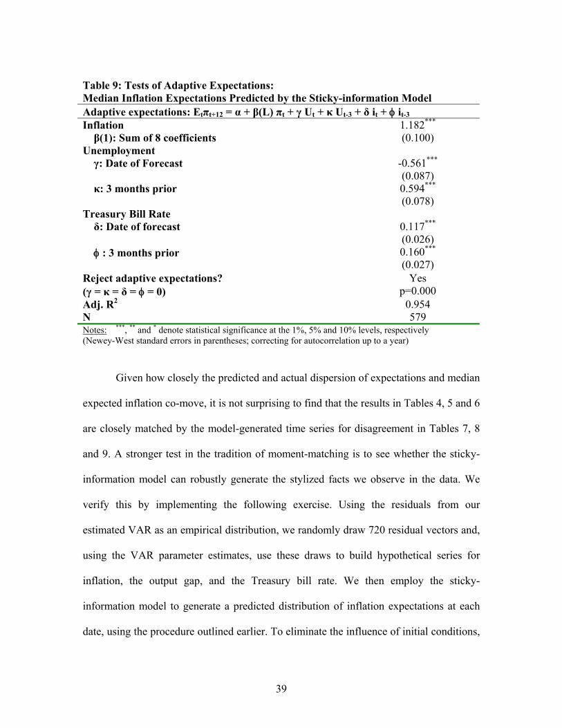
39

Table 9: Tests of Adaptive Expectations: Median Inflation Expectations Predicted by the Sticky-information Model Adaptive expectations: Etπt+12 = α + β(L) πt + γ Ut + κ Ut-3 + δ it + φ it-3 Inflation β(1): Sum of 8 coefficients

1.182*** (0.100)

Unemployment γ: Date of Forecast -0.561***

(0.087) κ: 3 months prior

0.594*** (0.078)

Treasury Bill Rate δ: Date of forecast

0.117*** (0.026)

φ : 3 months prior

0.160*** (0.027)

Reject adaptive expectations? (γ = κ = δ = φ = 0)

Yes p=0.000

Adj. R2 0.954 N 579 Notes: ***, ** and * denote statistical significance at the 1%, 5% and 10% levels, respectively (Newey-West standard errors in parentheses; correcting for autocorrelation up to a year)

Given how closely the predicted and actual dispersion of expectations and median

expected inflation co-move, it is not surprising to find that the results in Tables 4, 5 and 6

are closely matched by the model-generated time series for disagreement in Tables 7, 8

and 9. A stronger test in the tradition of moment-matching is to see whether the sticky-

information model can robustly generate the stylized facts we observe in the data. We

verify this by implementing the following exercise. Using the residuals from our

estimated VAR as an empirical distribution, we randomly draw 720 residual vectors and,

using the VAR parameter estimates, use these draws to build hypothetical series for

inflation, the output gap, and the Treasury bill rate. We then employ the sticky-

information model to generate a predicted distribution of inflation expectations at each

date, using the procedure outlined earlier. To eliminate the influence of initial conditions,

40

we discard the initial 10 years of the simulated series, so that we are left with 50 years of

simulated data. We repeat this procedure 500 times, thereby generating 500 alternative

50-year histories for inflation, the output gap, the Treasury bill rate, the median expected

inflation and the interquartile range of inflation expectations predicted by the sticky-

information model with λ=0.1. The regressions in Tables 4, 5 and 6, describing the

relationship of disagreement and forecast errors with macroeconomic conditions are then

re-estimated on each of these 500 possible histories, generating 500 possible estimates for

each parameter.

Table 10 reports the mean parameter estimates from each of these 500 histories.

Also shown (in parentheses) are the estimates at the 5th and 95th percentile of this

distribution of coefficient estimates. We interpret this range as analogous to a

bootstrapped 95% confidence interval (under the null that the sticky-information model

accurately describes expectations). These results suggest that the sticky-information

model robustly generates a positive relation between the dispersion of inflation

expectations and changes in inflation as we observe in the data. Also, as in the data, the

level of the output gap appears to be only weakly related to the dispersion of

expectations.

Yet, at odds with the facts, the model does not suggest a robust relationship

between the level of inflation and the extent of disagreement. To be sure, the relationship

suggested in Table 6 does occur in some of these alternative histories, but only in very

few. In the sticky-information model, agents only disagree in their forecasts of future

inflation to the extent that they have updated their information sets at different points in

the past. Given our VAR model of inflation, only changes over time in macroeconomic

41

conditions can generate different inflation expectations by different people. The sticky-

information model gives no reason to find a systematic relation between the level of

inflation and the extent of disagreement. This does not imply though that for a given

history of the world such an association could not exist, and for the constellation of

shocks actually observed over the past 50 years this was the case, as can be seen in

Table 7. Whether the level of inflation will continue to be related with disagreement is an

open question.

Table 10: Model-Generated Disagreement and Macroeconomic Conditions Multivariate

regression Bivariate

regressions Dependent Variable: Interquartile range of model-generated inflation expectations Constant 1.027***

(0.612 ; 1.508)

Inflation Rate -0.009

(-0.078 ; 0.061) -0.010

(-0.089 ; 0.071) ∆Inflation-squared 0.029***

(0.004 ; 0.058) 0.030***

(0.005 ; 0.059) Output Gap -0.019

(-0.137 ; 0.108) -0.023

(-0.163 ; 0.116) Joint Test on Macro Data Reject at 5% level in

98.2% of histories

Adj. R2 0.162 N 588 588 Notes: ***, ** and * denote statistical significance at the 1%, 5% and 10% levels, respectively. (The 5th and 95th percentile coefficient estimates across 500 alternative histories are shown in parentheses.) . Adj. R2 refers to the average adjusted R2 obtained in the 500 different regressions.

Table 11 compares the median of the model-generated inflation expectations

series with the artificial series for inflation and the output gap. The results with this

simulated data are remarkably similar to those obtained earlier. Panel A shows that

expectations are unbiased, although there are many possible histories in which biases (in

either direction) of up to a quarter of a percentage point occur. Panel B shows that

sticky-information expectations are typically inefficient, while Panel C demonstrates that

they induce persistent forecast errors. Panel D shows that sticky-information expectations

42

also fail to fully exploit available macroeconomic information, precisely as we found to

be true in the survey data on inflation expectations. The precise relation between different

pieces of macroeconomic data and expectation errors varies significantly across histories,

but in nearly all of them there is a strong relation. Therefore, while the coefficients in

Table 11 are not individually significant across histories, within each history a Wald test

finds that macroeconomic data is not being fully exploited 78.6% of the times. That is,

the set of macro data that sticky-information agents are found to under-utilize depends on

the particular set of shocks in that history.

43

Table 11: Tests of Forecast Rationality: Median Inflation Expectations Predicted by the Sticky-information Model over Simulated Histories Panel A: Testing for Bias: πt - Et-12πt = α Mean Error (Constant only)

0.057%

(-0.264 ; 0.369) Panel B: Is Information in the Forecast Fully Exploited? πt - Et-12πt = α + β Et-12πt β: Et-12 [πt] 0.308**

(0.002 ; 0.6971) α: Constant -1.018%

(-2.879 ; 0.253) Adj. R2 Reject Efficiency? α=β=0 Reject at 5% level in

95.4% of histories Panel C: Are Forecasting Errors Persistent? πt - Et-12πt = α + β (πt-12 - Et-24πt-12) β: πt-12-Et-24 [πt-12] 0.260***

(0.094 ; 0.396) α: Constant 0.039%

(-0.237 ; 0.279) Adj. R2 0.072 Panel D: Are Macroeconomic data fully exploited? πt - Et-12πt = α + β Et-12 [πt] + γ πt-13 + κ it-13 + δ Ut-13 α: Constant -0.617%

(-3.090 ; 1.085) β: Et-12 [πt] 0.032

(-0.884 ; 0.811) γ: Inflationt-13 0.064

(-0.178 ; 0.372) κ: Treasury Billt-13 0.068

(-0.185 ; 0.385) δ: Output Gapt-13 0.170

(-0.105 ; 0.504) Joint Test on Macro Data (γ=κ=δ=0) Reject at 5% level in

78.6% of histories Adj. R2 0.070 N 569 Notes: ***, ** and * denote statistical significance at the 1%, 5% and 10% levels, respectively. (The 5th and 95th percentile coefficient estimates across 500 alternative histories are shown in parentheses.) . Adj. R2 refers to the average adjusted R2 obtained in the 500 different regressions.

Table 12 tests whether sticky-information expectations could be confused for

adaptive expectations in the data. The results strongly reject this possibility. Sticky-

information expectations are significantly influenced by macroeconomic variables (in this

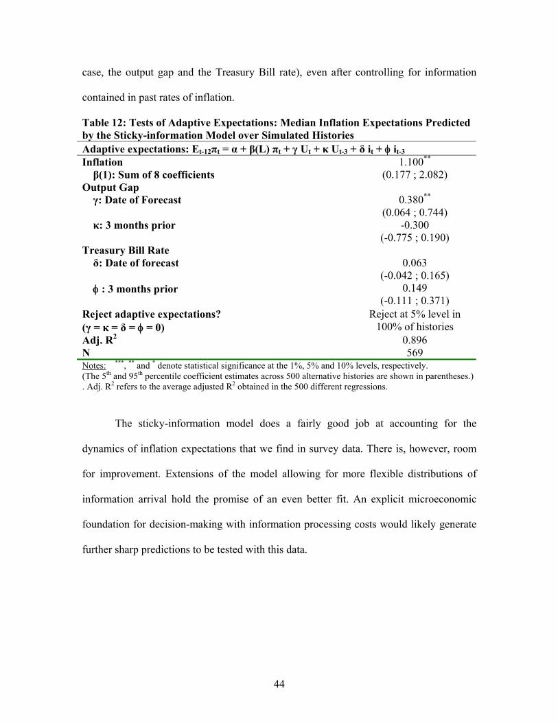
44

case, the output gap and the Treasury Bill rate), even after controlling for information

contained in past rates of inflation.

Table 12: Tests of Adaptive Expectations: Median Inflation Expectations Predicted by the Sticky-information Model over Simulated Histories Adaptive expectations: Et-12πt = α + β(L) πt + γ Ut + κ Ut-3 + δ it + φ it-3 Inflation β(1): Sum of 8 coefficients

1.100** (0.177 ; 2.082)

Output Gap γ: Date of Forecast 0.380**

(0.064 ; 0.744) κ: 3 months prior

-0.300 (-0.775 ; 0.190)

Treasury Bill Rate δ: Date of forecast

0.063 (-0.042 ; 0.165)

φ : 3 months prior

0.149 (-0.111 ; 0.371)

Reject adaptive expectations? (γ = κ = δ = φ = 0)

Reject at 5% level in 100% of histories

Adj. R2 0.896 N 569 Notes: ***, ** and * denote statistical significance at the 1%, 5% and 10% levels, respectively. (The 5th and 95th percentile coefficient estimates across 500 alternative histories are shown in parentheses.) . Adj. R2 refers to the average adjusted R2 obtained in the 500 different regressions.

The sticky-information model does a fairly good job at accounting for the

dynamics of inflation expectations that we find in survey data. There is, however, room

for improvement. Extensions of the model allowing for more flexible distributions of

information arrival hold the promise of an even better fit. An explicit microeconomic

foundation for decision-making with information processing costs would likely generate

further sharp predictions to be tested with this data.

45

VI. A CASE STUDY: THE VOLCKER DISINFLATION

In August of 1979, Paul Volcker was appointed chairman of the Board of

Governors of the Federal Reserve Board, in the midst of an annual inflation rate of 11%,

one of the highest in the post-war United States. Over the next three years, using

contractionary monetary policy, he sharply reduced the inflation rate to 4%.

This sudden change in policy and the resulting shock to inflation provides an

interesting natural experiment for the study of inflation expectations. The evolution of

the distribution of inflation expectations between 1979 and 1982 in the Michigan survey

is plotted in figure 12.13 For each quarter there were on average 2,350 observations in the

Michigan survey, and the frequency distributions are estimated non-parametrically using

a normal kernel smoothing function.

13 The Livingston and SPF surveys have too few observations at any given point in time to generate meaningful frequency distributions.

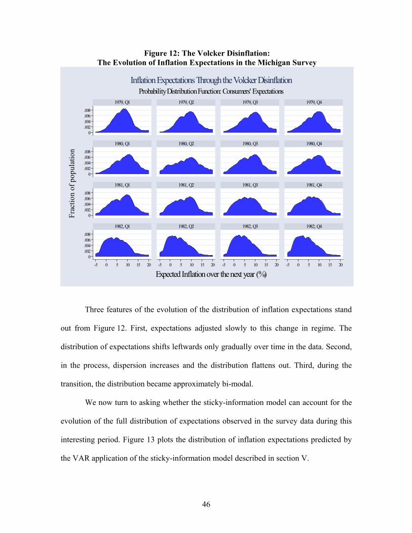
46

Figure 12: The Volcker Disinflation: The Evolution of Inflation Expectations in the Michigan Survey

0.002.004.006.008

0.002.004.006.008

0.002.004.006.008

0.002.004.006.008

-5 0 5 10 15 20 -5 0 5 10 15 20 -5 0 5 10 15 20 -5 0 5 10 15 20

1979, Q1 1979, Q2 1979, Q3 1979, Q4

1980, Q1 1980, Q2 1980, Q3 1980, Q4

1981, Q1 1981, Q2 1981, Q3 1981, Q4

1982, Q1 1982, Q2 1982, Q3 1982, Q4

Fra

ctio

n of

pop

ulat

ion

Expected Inflation over the next year (%)

Probability Distribution Function: Consumers' Expectations

Inflation Expectations Through the Volcker Disinflation

Three features of the evolution of the distribution of inflation expectations stand

out from Figure 12. First, expectations adjusted slowly to this change in regime. The

distribution of expectations shifts leftwards only gradually over time in the data. Second,

in the process, dispersion increases and the distribution flattens out. Third, during the

transition, the distribution became approximately bi-modal.

We now turn to asking whether the sticky-information model can account for the

evolution of the full distribution of expectations observed in the survey data during this

interesting period. Figure 13 plots the distribution of inflation expectations predicted by

the VAR application of the sticky-information model described in section V.

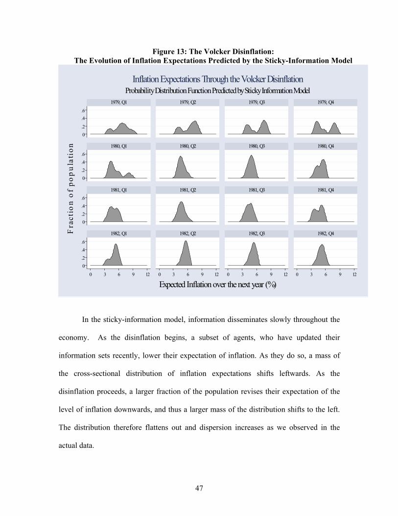
47

Figure 13: The Volcker Disinflation: The Evolution of Inflation Expectations Predicted by the Sticky-Information Model

0

.2

.4

.6

0

.2

.4

.6

0

.2

.4

.6

0

.2

.4

.6

0 3 6 9 12 0 3 6 9 12 0 3 6 9 12 0 3 6 9 12

1979, Q1 1979, Q2 1979, Q3 1979, Q4

1980, Q1 1980, Q2 1980, Q3 1980, Q4

1981, Q1 1981, Q2 1981, Q3 1981, Q4

1982, Q1 1982, Q2 1982, Q3 1982, Q4Fra

ctio

n o

f p

op

ula

tio

n

Expected Inflation over the next year (%)

Probability Distribution Function Predicted by Sticky Information ModelInflation Expectations Through the Volcker Disinflation

In the sticky-information model, information disseminates slowly throughout the

economy. As the disinflation begins, a subset of agents, who have updated their

information sets recently, lower their expectation of inflation. As they do so, a mass of

the cross-sectional distribution of inflation expectations shifts leftwards. As the

disinflation proceeds, a larger fraction of the population revises their expectation of the

level of inflation downwards, and thus a larger mass of the distribution shifts to the left.

The distribution therefore flattens out and dispersion increases as we observed in the

actual data.

48

The sudden change in inflation isolates two separate groups in the population. On

the one hand, there are those who have recently updated their information sets and are

now expecting much lower inflation rates. On the other hand, there remains a group

holding to pre-Volcker expectations, giving rise to a bi-modal distribution of inflation

expectations. As more agents become informed, a larger mass of this distribution shifts

from around the right peak to around the left peak. Ultimately, the distribution resumes

its normal single peaked shape, now concentrated at the low observed inflation rate.

Clearly the sticky-information model generates predictions that are “too sharp”.

Even so, it successfully accounts for the broad features of the evolution of the distribution

of inflation expectations during the Volcker disinflation.

VII. CONCLUSION

Regular attendees of the NBER Macroeconomics Annual conference are well

aware of one fact: People often disagree with one another. Indeed, disagreement about

the state of the field and the most promising avenues for research may be the conference's

most reliable feature. Yet, despite the prevalence of disagreement among conference

participants, disagreement is conspicuously absent in the theories being discussed. In

most standard macroeconomic models, people share a common information set and form

expectations rationally. There is typically little room for people to disagree.

Our goal in this paper is to suggest that disagreement may be a key to

macroeconomic dynamics. We believe we have established three facts about inflation

49

expectations. First, not everyone has the same expectations. The amount of disagreement

is substantial. Second, the amount of disagreement varies over time together with other

economic aggregates. Third, the sticky-information model, according to which some

people form expectations based on outdated information, seems capable of explaining

many features of the observed evolution of both the central tendency and the dispersion

of inflation expectations over the past fifty years.

We do not mean to suggest that the sticky-information model explored here is the

last word in inflation expectations. The model offers a good starting point. It is surely

better at explaining the survey data than are the traditional alternatives of adaptive or

rational expectations, which give no room for people to disagree. Nonetheless, the model

cannot explain all features of the data, such as the positive association between the level

of inflation and the extent of disagreement. The broad lesson from this analysis is clear: If

we are fully to understand the dynamics of inflation expectations, we will need to

develop of better models of information acquisition and processing. About this, we

should all be able to agree.

50

REFERENCES

Ball, Laurence (2000) “Near-Rationality and Inflation in Two Monetary

Regimes,” NBER Working Paper 7988.

Ball, Laurence and Dean Croushore (1995) “Expectations and the Effects of

Monetary Policy,” NBER Working Paper 5344.

Ball, Laurence, N. Gregory Mankiw and Ricardo Reis (2003) “Monetary Policy

for Inattentive Economies,” Journal of Monetary Economics, forthcoming.

Barnea A., A. Dotan and Josef Lakonishok (1979) “The Effect of Price Level

Uncertainty on the Determination of Nominal Interest Rates: Some Empirical Evidence,”

Southern Economic Journal.

Brenner, Menachem and Yoram Landskroner (1983) “Inflation Uncertainties and

Returns on Bonds,” Economica, pp. 463-468.

Bomberger, William and William Frazer (1981) “Interest Rates, Uncertainty and

the Livingston Data,” Journal of Finance, vol. 36 (3), pp. 661-675.

Bryan, Michael and Stephen Cecchetti (1994) “Measuring Core Inflation,” in N.

Gregory Mankiw, ed., Monetary Policy, Chicago: University of Chicago Press for NBER.

Bryan, Michael and Guhan Venkatu (2001) “The Curiously Different Inflation

Perspectives of Men and Women,” Federal Reserve Bank of Cleveland Economic

Commentary Series.

Carroll, Christopher (2003a) “Macroeconomic Expectations of Households and

Professional Forecasters,” Quarterly Journal of Economics, vol. 118 (1), pp. 269-298.

51

Carroll, Christopher (2003b) “The Epidemiology of Macroeconomic

Expectations,” in Larry Blume and Steven Durlauf, eds., The Economy as an Evolving

Complex System, III, Oxford University Press, forthcoming.

Croushore, Dean (1993) “Introducing: The Survey of Professional Forecasters,”

Federal Reserve Bank of Philadelphia, Business Review, November/December, pp. 3-15.

Croushore, Dean (1997) “The Livingston Survey: Still Useful After All These

Years,” Federal Reserve Bank of Philadelphia, Business Review, March/April, pp. 15-27.

Cukierman, Alex and Paul Wachtel (1979) “Differential Inflationary Expectations

and the Variability of the Rate of Inflation: Theory and Evidence,” American Economic

Review, vol. 69 (4), pp. 595-609.

Curtin, Richard (1996) “Procedure to Estimate Price Expectations,” mimeo,

University of Michigan Survey Research Center.

Friedman, Milton (1968) “The Role of Monetary Policy,” American Economic

Review, vol. 58 (1), pp. 1-17.

Gavin, William T. (2003) “FOMC Forecasts: Is All the Information in the Central

Tendency?” Federal Reserve Bank of St Louis Working Paper 2003-002A.

Juster, F. Thomas and Robert Comment (1978) “A Note on the Measurement of

Price Expectations,” Institute for Social Research Working Paper, University of

Michigan.

Khan, Hashmat and Zhenhua Zhu (2002) “Estimates of the Sticky-Information

Phillips Curve for the United States, Canada, and the United Kingdom,” Bank of Canada

Working paper 2002-19, forthcoming Journal of Money, Credit and Banking.

52

Llambros, Louis and Victor Zarnowitz (1987) “Consensus and Uncertainty in

Economic Prediction,” Journal of Political Economy, vol. 95 (3), pp. 591-62.

Levi, Maurice and John Makin (1979) “Fisher, Phillips, Friedman and the

Measured Impact of Inflation on Interest,” Journal of Finance, vol. 34 (1), pp. 35-52.

Lucas, Robert E., Jr. (1973) “Some International Evidence on Inflation-Output

TradeOffs,” American Economic Review, LXIII, pp. 326-334.

Makin, John (1982) “Anticipated Money, Inflation Uncertainty and Real

Economic Activity,” Review of Economics and Statistics, vol. 64 (1), pp. 126-134.

Makin, John (1983) “Real Interest, Money Surprises, Anticipated Inflation and

Fiscal Deficits,” Review of Economics and Statistics, vol. 65 (3), pp. 374-384.

Mankiw, N. Gregory and Ricardo Reis (2002) “Sticky Information Versus Sticky

Prices: A Proposal to Replace the New Keynesian Phillips Curve,” Quarterly Journal of

Economics, vol. 117 (4), pp. 1295-1328.

Mankiw, N. Gregory and Ricardo Reis (2003) “Sticky Information: A Model of

Monetary Non-neutrality and Structural Slumps,” in P. Aghion, R. Frydman, J. Stiglitz,

and M. Woodford, eds., Knowledge, Information and Expectations in Modern

Macroeconomics: In Honor of Edmund S. Phelps, Princeton University Press.

Mullineaux, Donald (1980) “Inflation Expectations and Money Growth in the

United States,” American Economic Review, vol. 70 (1), pp. 149-61

Souleles, Nicholas (2001) “Consumer Sentiment: Its Rationality and Usefulness

in Forecasting Expenditure – Evidence from the Michigan Micro Data,” forthcoming

Journal of Money, Credit and Banking.

53

Thomas, Lloyd, Jr. (1999) “Survey Measures of Expected U.S. Inflation,” Journal

of Economic Perspectives, vol. 13 (4), pp.125-144.

Vissing-Jorgenson, Annette (2003) “Behavioral Finance: An Impartial

Assessment or: Does Irrationality Disappear with Wealth? Evidence from Expectations

and Actions”, NBER Macroeconomics Annual, 2003.

54

Appendix: An Experimental Series for the Mean and Standard Deviation of

Inflation Expectations in the Michigan survey from 1946 to 2001

The Michigan Survey of Consumer Expectations and Behavior has been run most

quarters since 1946, Q1, and monthly since 1978. The current survey questions have

been asked continuously since January 1978 (see Curtin, 1996 for details):

Qualitative: “During the next 12 months, do you think that prices in general will go up, or

go down, or stay where they are now?”

Quantitative: “By about what percent do you expect prices to go (up/down) on the

average, during the next 12 months?”

For most of the quarterly surveys from June 1966-December 1976, an “open-ended”

version of the quantitative question was instead asked as:

Closed: “How large a price increase do you expect? Of course nobody can know for

sure, but would you say that a year from now prices will be about 1 or 2% higher, or 5%,

or closer to 10% higher than now, or what?”

Prior to 1966, the survey did not probe quantitative expectations at all, asking only the

qualitative question.

55

Thus, for the full sample period we only have a continuous series of qualitative

expectations. Moreover, even the exact coding of this question has varied through time

(Juster and Comment, 1978):

• 1948(1)-1952(1): “What do you think will happen to the prices of the things you

buy?”

• 1951(4), 1952(2)-1961(1): “What do you expect prices of household items and

clothing will do during the next year or so—stay where they are, go up or go

down?”

• 1961(2)-1977(2): “Speaking of prices in general, I mean the prices of the things

you buy—do you think they will go up in the next year or go down?”

• 1977(3)-Present: “During the next 12 months, do you think that prices in general

will go up, or go down, or stay where they are now?”

Lacking a better alternative, we proceed by simply assuming that these different question

wordings did not affect survey respondents.

We compile raw data for our experimental series from many different sources:

• 1948(1)-1966(1): Unpublished tabulations put together by Juster and Comment

(1978, Table 1).

• 1966(2)-1977(2): Tabulations from Table 2 of Juster and Comment (1978).

• 1967(2), 1977(3)-1977(4): Data were extracted from ICPSR studies #3619, #8726

and #8727, respectively.

• January 1978-August 2001: A large cumulative file containing microdata on all

monthly surveys. These data were put together for us by the Survey Research

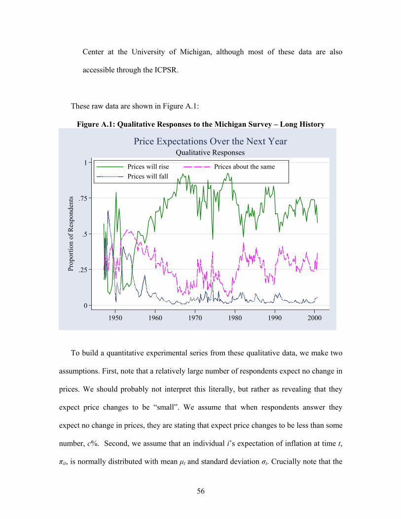
56

Center at the University of Michigan, although most of these data are also

accessible through the ICPSR.

These raw data are shown in Figure A.1:

Figure A.1: Qualitative Responses to the Michigan Survey – Long History

0

.25

.5

.75

1

Pro

port

ion

of R

espo

nden

ts

1950 1960 1970 1980 1990 2000

Prices will rise Prices about the same

Prices will fall

Qualitative ResponsesPrice Expectations Over the Next Year

To build a quantitative experimental series from these qualitative data, we make two

assumptions. First, note that a relatively large number of respondents expect no change in

prices. We should probably not interpret this literally, but rather as revealing that they

expect price changes to be “small”. We assume that when respondents answer they

expect no change in prices, they are stating that expect price changes to be less than some

number, c%. Second, we assume that an individual i’s expectation of inflation at time t,

πit, is normally distributed with mean µt and standard deviation σt. Crucially note that the

57

mean and standard deviation of inflation expectations are allowed to shift through time,

but that the width of the band around zero for which inflation expectations are described

as unchanged shows no intertemporal variation. (That is, there is no time subscript on c.)

Consequently, we can express the observed proportions in each category as a function

of the cumulative distribution of the standard normal distribution FN, the parameter c, and

the mean and standard deviation of that month’s inflation expectations, µt, and σt:

−−=

−−=

t

tNt

t

tNt

cFUp

cFDown

σµ

σµ

1%

%

Thus, we have two independent data points for each month (%Same is perfectly collinear

with %Up+%Down), and we would like to recover two time-varying parameters. The

above two expressions can be solved simultaneously to yield:

−−

=

−−−+

=

−−

−−

−−

)(%)%1(

2

)%1()(%

)%1()(%

11

11

11

tNtNt

tNtN

tNtNt

DownFUpFc

UpFDownF

UpFDownFc

σ

µ

Not surprisingly, we can recover the time series of the mean and standard

deviation of inflation expectations up to a multiplicative parameter, c; that is, we can

describe the time series of the mean and dispersion of inflation expectations, but the scale

is not directly interpretable. To recover a more interpretable scaling, we can either make

an ad hoc assumption about the width of the zone from which “same” responses are

drawn, or fit some other feature of the data. We follow the second approach and equate

the sample mean of the experimental series and the corresponding quantitative estimates

of median inflation expectations from the same survey over the shorter 1978-2001 period

58

when both quantitative and qualitative data are available. (We denote the median

inflation expectation by π~ .)14 Formally, this can be stated:

∑∑−−

=2001197820011978

~tt

t πµ , which solves to yield:

∑

∑−

−−

−−

−

−−−+

=20011978

11

11

20011978

)%1()(%

)%1()(%

~

t tNtN

tNtN

t

UpFDownF

UpFDownFc

π

This assumption yields an estimate of c=1.7%. That is, the specific scaling adopted

yields the intuitively plausible estimate that those expecting inflation between –1.7% and

+1.7%, respond that prices will “stay where they are now”. More to the point, this

specific scaling assumption is not crucial to any of our regression estimates. It affects the

interpretation of the magnitude of coefficients, but not the statistical significance.

Thus, for our sample of T periods, with 2T+1 parameters and 2T+1 unknowns, we

can estimate the time series of the mean and standard deviation of inflation expectations.

As a final step, we rely on the assumption of normality to convert our estimate of the

sample standard deviation into an estimate of the interquartile range.

Figures 1 and 3 show that the median and interquartile range of the constructed

series moves quite closely with the quantitative estimates over the period from 1978.

Table 2 reports on the correlation of this series with other estimates.

14 It is just as valid to refer to the mean of this experimental series as the median expectation, given the assumption of normality.