House price expectations

Discussion Paper

No.1829

February 2022

House price expectations

Niklas GohlPeter HaanClaus MichelsenFelix Weinhardt

ISSN 2042-2695

Abstract This study examines short-, medium-, and long-run price expectations in housing markets. We derive and test six hypothesis about the incidence, formation, and relevance of price expectations. To do so, we use data from a tailored household survey, past sale offerings, satellites, and from an information RCT. As novel findings, we show that price expectations exhibit mean reversion in the long-run. Moreover, we do not find evidence for biases related to individual housing tenure decisions or regret aversion. Confirming existing findings, we show that local market characteristics matter for expectations throughout, as well as aggregate price information. Lastly, we corroborate existing evidence that expectations are relevant for portfolio choice. Key words: housing, house price expectations JEL: R21; R31 This paper was produced as part of the Centre’s Urban Programme. The Centre for Economic Performance is financed by the Economic and Social Research Council. The authors thank Basit Zafar and Theodora Boneva for valuable feedback, as well as participants at various conferences and workshops. All remaining errors are our own. We gratefully acknowledge financial support by the German Research Foundation through CRC TRR 190. Niklas Gohl, DIW Berlin and Potsdam University. Peter Haan, DIW Berlin, FU Berlin and Netspar. Claus Michelsen, DIW Berlin, Leuphana University Lueneburg. Felix Weinhardt, European University Viadrina, DIW Berlin, CESifo, IZA and Centre for Economic Performance, London School of Economics. Published by Centre for Economic Performance London School of Economics and Political Science Houghton Street London WC2A 2AE All rights reserved. No part of this publication may be reproduced, stored in a retrieval system or transmitted in any form or by any means without the prior permission in writing of the publisher nor be issued to the public or circulated in any form other than that in which it is published. Requests for permission to reproduce any article or part of the Working Paper should be sent to the editor at the above address. N. Gohl, P. Haan, C. Michelsen and F. Weinhardt, submitted 2022.

1 Introduction

The behavior of housing markets has macroeconomic consequences. The sector itself

constitutes a sizeable share of GDP. Moreover, movements in house prices also have non-

negligible spillovers into other markets, e.g. on business investment or private consump-

tion, but also to the banking sector (see i.e. Iacoviello and Neri (2010); Duca et al. (2021)).

The housing market also has direct effects on the micro level. From the individual per-

spective, housing decisions are the most important financial decisions in the lives of most

people. As a result, understanding determinants of tenure decisions and housing markets

generally has long been in the focus of both micro- and macro- economists. For example it

is well understood that housing markets are characterized by short-run momentum (Case

and Shiller, 1989) and long-run mean reversion (Glaeser and Gyourko, 2006). However,

in contrast to the evidence about observed house market prices, the evidence about the

incidence and formation of price expectations is scare and speaks to the short or medium

run, see e.g. Armona et al. (2019) or Kindermann et al. (2021). Armona et al. (2019)

document momentum-effects in price expectations for periods up to five years. While five

years is a long period to form expectations over, in terms of housing cycles, five years is

rather short. Therefore, it is also important to understand long run price expectations.

This paper systematically examines the incidence, formation, and relevance of price

expectations over a period that captures a full housing cycle. Specifically, we study price

expectations over comprehensive periods relevant for housing markets: in the short-run

(2 years), medium-run (10 years), and the long-run (30 years). In the next section,

we derive six hypothesis regarding: (1) mean reversion, (2) individual characteristics

such as financial literacy, (3) tenure decisions, (4) local housing markets, (5) aggregate

information, and (6) the relevance of expectations for portfolio choice, which we then

empirically test in the data. The key finding of the paper is that while different factors

matter for price expectations over different time dimensions (discussed in detail below),

there is clear evidence for mean reversion in the long-run. Thus, we show that there is no

tension between price expectations and market cyclicality.

At the heart of our analysis is the design and inclusion of specific and novel housing-

1

related questions in a representative household panel survey, the Innovation Sample of the

German Socio Economic Panel (SOEP IS). We elicit beliefs and preferences, alongside a

rich set of individual and household characteristics, including detailed information about

current tenure and past tenure decisions. Specifically, in the survey, we ask representative

households about their expectations about the development of house prices in their cur-

rent neighborhood over a horizon of 2, 10, and 30 years, respectively. Besides these novel

questions, respondents also complete the SOEP-core questions, meaning that we have ac-

cess to an unusually large set of individual- and household-level background characteristics

that might affect the formation of price expectations, including measures of educational

background and financial literacy. For our analysis, we augment the survey-information

further and merge with a number of additional data sets: local data on housing prices, as

well as satellite data and remotely sensed terrain data to construct an index of housing

supply in the spirit of Saiz (2010). These additional data allow us to study how price

expectations correlate with local housing market characteristics. Finally, we conduct a

randomized information treatment in which one part of the respondents is given infor-

mation about historical housing price developments. We use this setup to study causal

effects of information provision on expectations and on a hypothetical portfolio choice

outcome.

Our first important finding is that there exists strong evidence for mean reversion

of price expectations in the long-run. For short time-horizons, our results confirm the

existing empirical literature on momentum-effects. However, for the horizon of thirty years

individuals do not expect a long run increase in house prices. Notably, these expectations

can be reconciled with mean reversion in markets (Glaeser and Gyourko, 2006) and the

historical incidence of cycles: Bracke (2013) shows that housing cycles have become longer

over time, with the last global cycle lasting for about twenty years. Our further findings

show that individual characteristics have a modest effects on expectations. This holds for

the short run, the medium run, and the long run. Females are more conservative and the

well-educated have slightly lower expectations for the short run but higher expectations

in the longer term. We refute our third hypothesis related historical decisions and regret

2

aversion: we find that the own tenure status does not correlate with expectations. On

the other hand, consistent with Kindermann et al. (2021), our results show that renters

who have experienced a recent rental rise have higher price expectations. Examining the

role of local markets, we find that local price trends have very strong predictive power

for local expectations in the short term. Over the long term, land supply, as stipulated

by housing market theories, plays a key role in predicting expectations. However, in line

with recent empirical literature, our findings also document that individuals factor in more

aggregate, distant information, such as past aggregate OECD-level trends, when forming

expectations. This fifth hypothesis is tested using an information RCT that presents data

on past (averaged) price developments of OECD countries. Finally, we show that this

information RCT also shows effects on a portfolio choice question.

This paper is related to a new and quickly growing literature that examines how price

expectations are formed in the housing market and if these affect individual behavior. In

particular, Kuchler and Zafar (2019) show that individuals use regional price trends to

form expectations about future prices at the national level. In a different context, Bailey

et al. (2018) show that housing decisions of distant friends on Facebook have effects

on local behavior. Niu and van Soest (2014) show that medium run expectations are

positively related to past house price developments and perceived economic conditions.

Kindermann et al. (2021), focusing on short term price expectations in Germany, find

that renters have higher and more accurate price expectations. In a quantitative model,

they explain the difference and show that renters are relatively well informed about house

prices. Most closely related to this study, Armona et al. (2019) study how local market

conditions and information affect the formation of price expectations. They find that local

markets have strong effects on individual’s expectations in the short- and medium-run,

without any evidence for mean reversion. Moreover, they show that information about

markets affects expectations and stated investment decisions. So far, most studies consider

price expectations in the short- or medium-run. For example, Armona et al. (2019) find

evidence for momentum-effects over one-year periods, with no evidence for mean-reversion

for periods of up to five years. While five years is a long period to form expectations over,

3

in terms of housing cycles, five years might not be long enough. Whether evidence for

psychological driven volatility or momentum-effects (Shiller, 2015, e.g.) persists in price

expectations also over longer time-horizons is an open question.1 Moreover, there exists

no evidence how individual characteristics such as education, numeracy, tenure type or

local housing market characteristics affect the price expectations over longer horizons.

This study starts filling this gap.

The paper is structured as follows: the next section describes the hypotheses tested

in this study in more detail. Section 3 gives a brief overview of the German housing

market and introduces the data sets used in the paper. Section 4 describes the empirical

setting of our study. In section 5 and 5.2 we present our results and robustness checks,

respectively. Lastly, section 6 concludes.

2 Formation of expectations: derivation of hypothesis

First hypothesis: Mean reversion in the long run The existing literature (Armona

et al., 2019) finds evidence for momentum-effects for price expectations in the short-

run (i.e. after one-year) with no evidence for mean-reversion for periods of up to five

years (medium-run). However, there is ample evidence that housing cycles exist and

that markets show mean-reversion over longer periods, i.e. Wheaton (1999); Glaeser and

Gyourko (2006). Given the duration of the most recent cycles (Bracke, 2013), we do not

necessarily expect to see evidence for mean reversion over ten years -but certainly over

the thirty-year period momentum-effects should not dominate. Therefore we hypothesize

that we will find evidence for mean reversion in long-run expectations.

Second hypothesis: The role of individual characteristics Individual character-

istics can influence expectations in the short-, medium-, and long-run. A large literature

documents gender-differences in willingness to take financial risks (Charness and Gneezy,

2012; Almenberg and Dreber, 2015, e.g.). Applied to the formation of expectations, we

hypothesize that males are more likely to hold large and positive price expectations, see1Forming expectations over longer periods is not problematic per se: answering to a very similar

question on wages the individuals that we study are able to form accurate expectations over thirty years.

4

e.g. Breunig et al. (2021). A second individual factor that may influence the formation of

expectations is the level of education. More highly educated individuals should be better

in processing information for the formation of price expectations. Behavioral biases, such

as not compounding interests and financial illiteracy, are shown to diminish with better

education, see e.g. Lusardi (2008). We test this hypothesis using educational information

(the highest educational degree obtained) and information about the financial literacy

and self-assessed numeracy of the individual.

Third hypothesis: The role of housing and tenure The own housing and the

tenure situation may affect the expectations of prices. In particular, owner-occupiers

could be more optimistic compared to renters - simply because they partly select into

the respective housing tenure based on their expectations. Equally, reference point the-

ory would suggest that past decisions could have additional influences on the formation

of expectation: Individuals who have purchased a home (owner-occupiers) might not

downward-adjust expectations to rationalize past decisions ex-post, see e.g. Lamorgese

and Pellegrino (2019); Genovese and Mayer (1997). More generally due to an “endow-

ment effect,” (List, 2011) homeowners might attach a greater value to their home, see e.g.

Goodman et al. (1992); Chan et al. (2016); Bao and Gong (2016). Similarly, homeown-

ers who decide against selling at times of relatively high housing prices might experience

regret aversion and, consequently, would rather not consider selling their house, see e.g.

Seiler et al. (2008). On the other hand, individuals who decided against buying might

be reluctant to enter the market at higher prices, to avoid the feeling of regret of not

having bought earlier at lower prices. For renters, having experienced rental rises might

lead to higher expectations. In sum, selection into owner-occupation as well as behavioral

biases (endowment effects, regret aversion) would suggest that owner-occupiers should

hold more positive price expectations compared to renters. Expectations of renters, on

the other hand, could be affected by recent rental rises. This, in turn, could lead to higher

price expectations of renters (Kindermann et al., 2021).

5

Fourth hypothesis: The role of local housing markets We explore the hypothesis

that local housing markets matter for the formation of expectations in the short-, medium-

, and long-run by testing the effect of past local prices trends and the effect of local housing

supply on expectations. The hypothesis is motivated by previous literature, as studies

show that past local prices trends to positively affect price expectations for periods of up

to five years; see e.g. Case et al. (2012); Niu and van Soest (2014); Armona et al. (2019).

In addition, the elasticity of land is shown to play a key role for long-run housing supply

and house price developments (Saiz, 2010). In theory, more available land for residential

development should dampen future price increases. This could also be the case when

examining price expectations, in particular for the long-run.

Fifth hypothesis: The role of aggregate information The literature highlights

that information, such as housing decisions of distant friends on Facebook, affects local

behavior; see e.g. Bailey et al. (2018). Further, Kuchler and Zafar (2019) show that

local price trends significantly shape national, aggregate house price expectations. We

hypothesize that information on past aggregate house price development affects expec-

tations. Specifically, we test if information on residential real estate prices in 14 differ-

ent countries, including Germany and the United States, that on average approximately

quadrupled since 1945, has a positive effect on individual house price expectations. We

test this using an RCT, which we describe further in Section 3.

Sixth hypothesis: The relevance of expectations for investment decisions In

the final hypothesis, we move beyond the formation of expectations and directly test if

expectations about house prices affect planned investment. To provide a causal answer

to this question, we estimate if information on past aggregate house price developments

(see hypothesis five), which we provide using an RCT, affects stated investment decisions

of individuals.

6

3 Institutional Background and Data

3.1 The German Housing Market

In comparison to most OECD countries, the German housing market has a relatively

low share of homeownership, with owner-occupied dwellings accounting for less than half

of all occupation forms (Voigtlaender, 2010). In rural and suburban areas, especially in

eastern Germany, the housing market is relatively stable. In contrast, in urban agglom-

erations and student cities, severe housing shortages dominate the local housing markets,

ultimately putting upward pressure on housing prices in these areas (Kholodilin et al.,

2016). However, even within big cities, substantial variations in local housing markets ex-

ist (BMF, 2017, .5). The regional differences in the German housing market are, in turn,

reflected in rent and house price developments. Particularly, since 2007/2008, housing

prices have strongly increased in popular urban areas, including the Big Seven cities2 but

stagnated or only increased marginally in many rural areas. The German context hence

offers rich variation, making it a relevant setting for the study of the formation of price

expectations.

3.2 Data

3.2.1 The German Socioeconomic Panel Innovation Sample

SOEP-IS For the analysis, we use a range of different data sets. The main data set

is the German Socioeconomic Panel’s innovation sample (SOEP IS). The SOEP IS an

annual representative survey providing information on a large set of socioeconomic and

demographic variables and specific survey modules, see Richter and Schupp (2015) and

Goebel et al. (2019). As part of the SOEP IS waves in 2016-2018, we were able to design

a specific module of questions to elicit price expectations of households. For this analysis,

the questions on the short-, medium-, and long-term formation of house price expectations

of individuals are of central interest. In all waves, we ask for expectations of local housing

prices over a two and thirty year horizon. More precisely, individuals were asked the2Berlin, Hamburg, Munich, Cologne, Duesseldorf, Frankfurt am Main, and Stuttgart

7

following question:

The following section focuses on your expectations of house price developments in your

area. In your opinion: How will house prices develop in comparison to today?

Participants then had the option to state whether prices will fall, rise, remain the same

or not answering at all. Depending on their answer individuals were asked By how much -

in percent- do you think prices will fall/rise. For the 2017 wave, we additionally asked for

expectations over a ten year horizon. Crucially, the survey is regionally representative,

sampling individuals from a total of 183 postal codes covering 75 out of 90 residential

postal code regions in Germany (see Figure A.3).

In addition, the SOEP IS data provides a wide range of socioeconomic variables. For

example, individuals were asked to assess their own math skills as rather proficient or

rather bad. Further, individuals received several questions testing their financial literacy.

Based on the answer, we construct a measure of financial literacy; see Grohmann et al.

(2019).3

3.2.2 RCT on past aggreagate price trends

To test the importance of aggregate house price information, we designed a random-

ized controlled information trial that we could implement within the SOEP IS household

survey. As part of the RCT, we provide randomly selected survey participants with

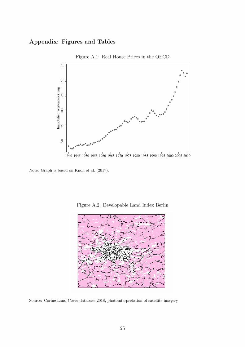
background information on past aggregate housing price developments, see Figure A.1.

Additionally, the treatment group received the information that the graph depicts the

development of average prices in residential real estate in 14 different countries, including

Germany and the United States, and that prices on average approximately quadrupled3More precisely, individuals were asked the following three questions:

1. Assume the interest of your savings account is 1% per year and the inflation rate is 2% per year.What do you think: One year from now, could you buy the same, more, or less than today withthe credit at your savings account (Answer options: More, less, the same, I do not know).

2. Assume that you have a 100 euros deposit in your savings account. This credit bears interest at 2%per year and you leave it on this account for 5 years. How much credit will your savings accounthave after 5 years? (Answer options: More than a 102 euros, less than a 102 euros, Exactly a 102euros, I do not know)

3. Is the following statement correct or wrong? The investment into shares of one company is lessrisky than into an equity fund.

8

since 1945. In the 2018 wave of the SOEP IS, we repeated the RCT for the same individ-

uals.

In the 2018 wave, individuals were additionally asked to allocate assets between dif-

ferent investment options. More precisely, participants were asked the following:

Suppose you have some spare money and have decided to invest this money. How would

you in per cent allocate your money between the following investment options? The given

options were stocks, real estate, state bonds, savings account, and gold.

3.2.3 Postal code, house price and land supply data

We use three additional data sets to obtain information on regional demographics and

housing markets. First, we use the empirica ag housing data bank for the years 2012 to

2016 (pre-period) to derive postal code specific hedonic regional house price trends. The

empirica ag data bank contains all listings and deals from 2012 to 2016 conducted through

Germany’s largest online real estate platforms such as Immoscout and immowelt/immonet,

newspapers and local online platforms. In total, the data bank provides 484,604 observa-

tions for rental and non-rental properties over the given time period. Table A.1 provides

summary statistics of the observed transaction prices. In addition, the data base offers a

wide range of background information on the listed properties such as the dwelling’s size,

age, state, room number and equipment . We use this information to construct hedonic,

quality-adjusted average annual house price trends for each postal code over the 2012-2016

period4. The quality-adjusted trends are one indicator that we employ to assess how local

housing markets impact housing expectations.

As a second indicator, we construct a postal code specific developable land index that

serves as a proxy for local housing supply elasticity. For this, we use Corine Land Cover

2018 data to identify land that is potentially developable. The Corine Land Cover data

is based on 100m resolution satellite data that, via remote sensing, provides the basis for

over 37 land cover and land use categories, such as sports and leisure facilities or wetlands.

Using this information, we construct an index of developable land supply for Germany4Figure A.3 in the Appendix depicts the hedonic price trends for each postal code region in Germany.

9

similar to Saiz (2010).5 As an example, Figure 1 depicts the index as constructed for

Berlin and surroundings. The pink areas show land that is potentially developable. As

expected, more land is developable in the rural areas surrounding Berlin, whereas within

the city itself developable land is relatively scarce. Lastly, in order to control for postal

code specific characteristics, such as population density, we use Census data.6

4 Empirical Approach

The empirical approach follows directly from the hypotheses presented in Section 2. The

first set of results that we use to test the first hypothesis is descriptive in nature and we

take great care in establishing representativeness of our respondents.

In order to test the relation between house price expectations and the impact of

individual characteristics, housing/tenure, information, as well as local housing markets,

respectively, we adopt the empirical framework described in Equation 1. Yi are the two,

ten, and thirty year expectation outcomes, respectively. Depending on the hypothesis we

seek to test, we separately include sets of different explanatory variables.

First, in order to assess the role of individuals characteristics, we regress the expec-

tation outcomes on Ci, which is a matrix of individual characteristics, like the level of

education, gender, as well as variables measuring financial literacy and self-assessed nu-

meracy skills.

Secondly, we regress the expectation outcomes on housing and tenure characteristics

contained in Hi, such as the tenure choice and past rental increases.

Thirdly, we test the impact of local housing market experiences and run the regression

on measures for the local housing market (i.e. Li) at the postal code level, such as an

average hedonic price trend and the land supply index described above.

Finally, in order to analyze the role of information, we regress the expectation outcomes5We abstract from zoning decisions due to a lack of data, but see these as potentially malleable in the

long run anyway. Accordingly, we classified as developable all categories that could be used for supply,in principle: Non-irrigated arable land; Vineyards; Fruit trees and berry plantations; Pastures; Complexcultivation patterns; Land principally occupied by agriculture, with significant areas of natural vegetation;Agro-forestry areas; Broad-leaved forest; Coniferous forest; Mixed forest; Natural grasslands; Moors andheathland; Transitional woodland-shrub; Beaches, dunes, sands; Bare rocks; Sparsely vegetated areas.

6Note that the last Census was conducted in 2011. Data on population size is available.

10

on a variable indicating whether the individual received the information treatment, Ii.

Here, we naturally restrict our sample to the years in which the RCT was conducted, i.e.

2017 and 2018. In addition, we use a portfolio choice question asked in 2018 as another

outcome variable to complement the analysis and to test if expectations have an effect on

behavior.

Yi = β0 + C ′iβ1 +H ′

iβ2 + β3Ii + L′iβ4 + β5 +

Y∑y

ηy +R∑r

θr + ui (1)

Depending on the specification, we control for the year of the survey by including year

fixed effects, ηy. Further, in order to control for potential unobserved regional variation

in expectations and housing markets, we include commuting zone fixed effects, i.e. θr.

Commuting zones are based on the so called Raumordnungsregionen provided by the Ger-

man government. In total there are 96 of these regions across Germany. Crucially, the

commuting zones are larger than postal codes in Germany, which, in turn, allows us to

exploit the within commuting zone variation whilst controlling for time-invariant unob-

servables at the commuting zone level. This is crucial since there might be unobservable

characteristics that simultaneously are correlated to price expectations and local housing

market performance. Further, we control for a range of individual and postal code covari-

ates contained in X. More precisely, when appropriate, we control for the information

treatment half of the participants in the 2017 and 2018 samples received. In addition we

control for age, personal income, and the postal code log population density.

5 Results

5.1 Main Results

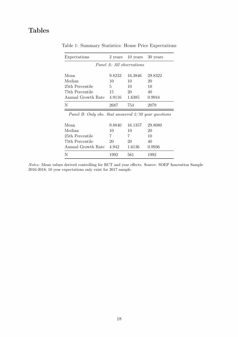
Price expectations and mean reversion in the long run (H1) Table 1 provides

summary statistics for house price expectations in two, ten, and thirty years. As previ-

ously described, expectations over ten years were only part of the survey in 2017. Thus,

observation numbers are smaller by construction for this outcome. For the two and thirty

11

year outcomes, it is important to note that more individuals (2687 vs. 2079) answered

the question over the shorter time frame than over the long horizon. In order to ensure

that there is no systematic difference in the expectation outcomes stated by those who

answered only one question, in addition to the summary statistics for all observations

(Panel A), we provide results for survey participants who only answered the questions on

two and thirty year expectations (Panel B).

On average individuals expect house prices to increase by just under 10 percentage

points in the next two years, which corresponds to an average annual growth rate of just

under 5 percentage points. Over a ten year horizon individuals on average expect an

increase of more than 16 percentage points. This corresponds to an annual growth rate

of approximately 1.6 percentage points. Over a thirty year frame, the survey participants

expect prices to increase by only about 30 percentage points with an annual growth rate

of about one percent. Crucially, there is no substantial difference between the results of

Panels A and B. Thus, we continue our analysis using the answers of all respondents.

Examining the annual growth rates in Table 1, it is immediately clear that the longer

the time horizon over which the expectations are given, the lower the corresponding an-

nual growth rate. Figure A.4 represents this finding graphically and depicts hypothetical

linear growth trajectories based on the respective annual growth rates derived from the

different time frames over which expectations were collected. Crucially, we assume a

constant annual growth to calculate the growth trajectories. For example, based on an

annual growth rate of just under five percent derived from the two year time frame, the

corresponding 30 year ahead forecast under the assumption of constant annual growth is

a 147.35. Asked over a ten year time frame, the 30 year ahead forecast is reduced to less

than a third of the answer, i.e. 49.15, and for a time frame of 30 years, we obtain an

average forecast of just under 30 percent. The black triangle indicates the actual expec-

tations stated when directly asked about the relevant time frame and, hence, corresponds

to the mean values stated in Panel A of Table 1. Most importantly, we see that the

growth trajectories become flatter the longer the time horizon over which expectations

are elicited. Therefore, the results suggest patterns of mean reversion in the long term

12

house price expectations, a result that is frequently shown empirically for actual house

prices, see e.g. Gao et al. (2009), and is consistent with findings of elastic housing supply

responses in the long run, see e.g. Green et al. (2005); Saiz (2010); Glaeser et al. (2014).

In Table A.2 in the Appendix, we provide heterogeneous results by different charac-

teristics such as gender, education, and tenure type. Most importantly, patterns of mean

reversion hold across all types.

The role of individual characteristics (H2) Table 2 depicts regressions of the dif-

ferent house price expectation outcomes on a range of individual socioeconomic variables

frequently suggested in the literature to be central for the formation of price expectations

(see Section 2). More precisely, Table 2 depicts the regression results for the different

expectation outcomes on a female dichotomous variable, a college indicator variable, and

a numeracy dummy. The numeracy dummy indicates whether individuals would classify

their math skills as rather proficient. Further, we include three variables testing financial

literacy. Depending on the specification, we include the potential explanatory variables

without controls or we include the full set of control variables and the commuting zone

and year fixed effects.

Individuals with a college degree, on average, have significantly lower short-run expec-

tations of about 1.74 percentage points when including the full set of controls. Conversely,

women appear to be less optimistic in the medium- to long-run, with significantly lower

expectations over the ten and thirty year horizon. The self-assessed numeracy skill is

significant over the medium- and long-run. The Financial Literacy indicator, shows a

slightly significant point estimate in the short term, indicating that individuals who grasp

the concept of compound interest have slightly lower expectations in the short term. The

estimate, however, is only significant at the ten percent level. All in all, there is limited

evidence that individuals with higher self-assessed math skills, expect higher increases

in house prices. Surprisingly, only the financial literacy indicator for the interest rate

question is significant at the ten percent level, indicating that individuals who answered

the question correctly expect prices to increase less strongly over the 2 year horizon.

Our findings overall are in line with previous findings that document more pessimistic

13

expectations amongst women. Further, they support the hypothesis that, to a limited

extent, education, financial literacy, and numeracy play a role in shaping expectations,

which is consistent with Kindermann et al. (2021).

The role of housing and tenure (H3) In Table 3, we focus on the effect of hous-

ing and tenure features and regress the respective expectation outcomes and whether

the monthly rental payment was increased during the last four years. The tenure type,

i.e. owning or renting, does not appear to play a role in explaining differences in ex-

pectations. The results are at odds with frequently documented endowment effects for

different markets, including the housing market. For example, homeowners are shown

to over-estimate the value of their homes (see Kahneman et al. (1990), Goodman et al.

(1992), Bao and Gong (2016), Chan et al. (2016)). In light of this literature, we would

expect a higher expected house price change by homeowners. However, the results in

Table 3 show that there does not appear to be a significant difference in homeowners and

tenants expectations regardless over which time frame.

In turn, tenants who experienced a rental increase in the past four years, have higher

expectations. However, when including the full set of covariates, only the point estimate

for the ten year horizon is statistically significant.

The role of local housing markets (H4) In a next step, we test if local housing

market conditions affect future housing price expectations. In Table 4, we regress house

price expectation on the measures of local housing market performance described above.

The average yearly postal code specific hedonic price trend as well as the postal code

specific housing supply index constructed from satellite data are significant in predicting

short term expectations when not including control variables. When including controls

and fixed effects only, the coefficient of the price trend remains significant at the five

percent level. This estimate is in line with findings of Kuchler and Zafar (2019), who,

depending on the specification, present estimates for one year ahead expectations of about

0.886, albeit for a regression of local price changes on nationwide house price expectations.

When looking at the 10 and 30 year house price expectations, the supply index gains in

14

absolute size and significance, particularly over the long-term horizon of 30 years. In

contrast, when including fixed effects and control variables, the price trend point estimate

no longer is significantly different from zero. The sizable and significant effect of the supply

index is consistent with theories and empirical evidence assuming housing supply to be

elastic in the long-run, see e.g. Saiz (2010). In our context, an increase of the land supply

index by one percentage point indicates more developable land in the respective postal

code and, hence, a more elastic supply response in the housing market. Thus, standard

theory would suggest lower house prices as a consequence of a more elastic supply response.

This is confirmed by our results. Overall, the results suggest that individuals observe

local market conditions and take them into consideration when forming expectations.

Particularly, the supply index appears to be relevant for long-run expectations. Past

price developments, as indicated by our regression results, in turn, appear to play only a

role in the short-run.

The role of information on expectations (H5) In Panel A of Table 5, we report re-

gression results of the expectation outcomes on the randomly assigned information treat-

ment. The treatment showed aggregate and long-run price developments. The results

show that individuals in the treatment group, on average, expect stronger price increases

in the short- and long-run. However, the coefficients of the treatment variable in the

short-run specification are statistically insignificant with p-values above the 10 percent

level of significance. The coefficient in the long-run specification, however, is significant

at the ten percent level. When including the additional control variables and fixed effects,

the point estimate decreases and is no longer significant. Overall, the results suggest

that, on average, treated individuals approximately expect higher long-run price changes.

Thus, in the long-run aggregate long-run information appears to matter when forming

expectations about future house price developments, although not very much. The result

confirms findings, see e.g. Bailey et al. (2018), that, in addition to local information, indi-

viduals also factor in more distant, aggregate information, such as pooled average OECD,

long-run price developments used as an information treatment in our setting. However,

such effects do not appear strong enough to counter-act the mean reversion observed in

15

the long-run.

The relevance of expectations for stated decisions (H6) As described in Section

2, we also use the RCT to test the relevance of expectations on a hypothetical portfolio

investment question that was asked in 2018. Panel B in Table 5 depicts the regression

results for this new outcome.

The key finding is that, on average, individuals who received the information treat-

ment invest relatively more in housing. However, the estimated coefficient is no longer

significant when including commuting zone fixed effects, which might be due to the rela-

tively small number of observations and, hence, a low within commuting zone variation.

Overall, our findings provide slightly imprecise, albeit causal, evidence that long term

expectations can matter for investment decision, thereby confirming findings of Kuchler

and Zafar (2019).

5.2 Robustness checks

In the Appendix, we provide robustness checks for all hypothesis tests. First, we repeat

our estimations for standard errors clustered at the commuting zone level. Secondly, we

seek to shed light on whether the expectation outcomes can be interpreted in nominal or

real terms. Our results are robust to clustering decisions as well as to interpretations of

questions regarding inflation.

6 Discussion and conclusions

In this paper, we test six sets of hypothesis regarding price expectations over different time

horizons. To do this, we develop survey questions to elicit information on how individuals

form house price expectations. Specifically, we design questions focusing on the long-run

expectations in thirty years, a time horizon that is crucial for investment/tenure decisions

and that is not extensively studied in the literature on house price expectations.

As our key finding, the empirical analysis shows that, in the long-run, individual house

price expectations show patterns of mean reversion. Further, we show that most tenure

16

decisions are not significantly correlated with future price expectations, whereas individual

characteristics, such as gender and education, as well as local housing market experiences,

play a key role. A land supply proxy constructed from satellite data is strongly correlated

with (long-term) price expectations.

We also replicate a range of empirical findings from the literature, mostly from the US,

in the context of Germany. This shows that Germans in the short- to medium-run behave

similarly when forming house price expectations. Most importantly, we document short-

run momentum effects. All in all, our findings are generally consistent with empirically

observed and theoretically formulated models of housing cycles that document short-run

momentum effects and long-run mean reversion.

17

Tables

Table 1: Summary Statistics: House Price Expectations

Expectations 2 years 10 years 30 years

Panel A: All observations

Mean 9.8232 16.3846 29.8322Median 10 10 2025th Percentile 5 10 1075th Percentile 15 20 40Annual Growth Rate 4.9116 1.6385 0.9944

N 2687 754 2079

Panel B: Only obs. that answered 2/30 year questions

Mean 9.8840 16.1357 29.8080Median 10 10 2025th Percentile 7 7 1075th Percentile 20 20 40Annual Growth Rate 4.942 1.6136 0.9936

N 1992 561 1992

Notes: Mean values derived controlling for RCT and year effects. Source: SOEP Innovation Sample2016-2018; 10 year expectations only exist for 2017 sample.

18

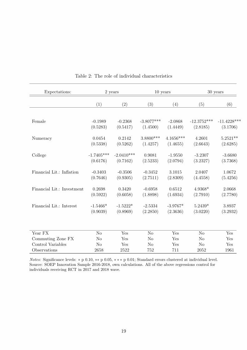
Table 2: The role of individual characteristics

Expectations: 2 years 10 years 30 years

(1) (2) (3) (4) (5) (6)

Female -0.1989 -0.2368 -3.8077*** -2.0868 -12.3752*** -11.4228***(0.5283) (0.5417) (1.4500) (1.4449) (2.8185) (3.1706)

Numeracy 0.0454 0.2142 3.8800*** 4.1656*** 4.2601 5.2521**(0.5338) (0.5262) (1.4257) (1.4655) (2.6643) (2.6285)

College -1.7405*** -2.0410*** 0.9081 -1.9550 -3.2307 -3.6680(0.6176) (0.7162) (2.5233) (2.0794) (3.2327) (3.7368)

Financial Lit.: Inflation -0.3403 -0.3506 -0.3452 3.1015 2.0407 1.0672(0.7646) (0.9305) (2.7511) (2.8309) (4.4558) (5.4256)

Financial Lit.: Investment 0.2698 0.3420 -0.6958 0.6512 4.9368* 2.0668(0.5922) (0.6058) (1.8898) (1.6934) (2.7910) (2.7780)

Financial Lit.: Interest -1.5466* -1.5222* -2.5334 -3.9767* 5.2439* 3.8937(0.9039) (0.8969) (2.2850) (2.3636) (3.0220) (3.2932)

Year FX No Yes No Yes No YesCommuting Zone FX No Yes No Yes No YesControl Variables No Yes No Yes No YesObservations 2658 2522 752 711 2052 1961

Notes: Significance levels: ∗ p 0.10, ∗∗ p 0.05, ∗ ∗ ∗ p 0.01; Standard errors clustered at individual level.Source: SOEP Innovation Sample 2016-2018, own calculations. All of the above regressions control forindividuals receiving RCT in 2017 and 2018 wave.

19

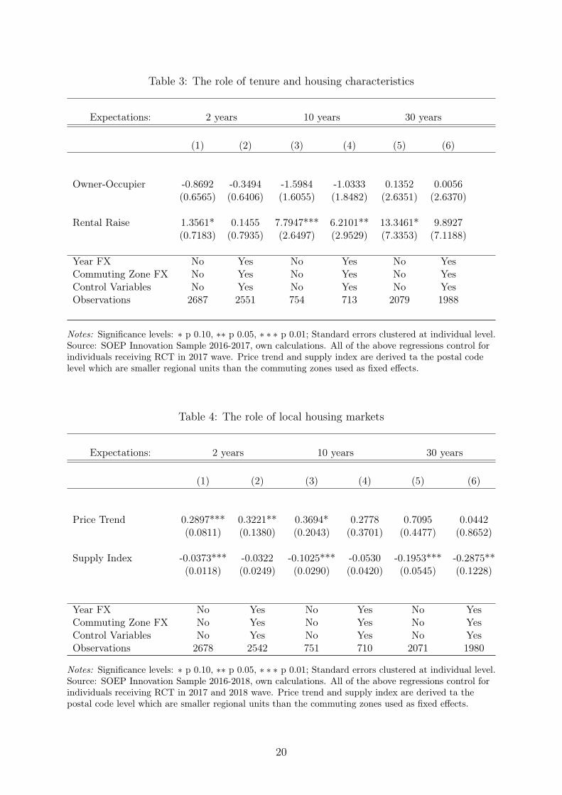
Table 3: The role of tenure and housing characteristics


(1) (2) (3) (4) (5) (6)

Owner-Occupier -0.8692 -0.3494 -1.5984 -1.0333 0.1352 0.0056(0.6565) (0.6406) (1.6055) (1.8482) (2.6351) (2.6370)

Rental Raise 1.3561* 0.1455 7.7947*** 6.2101** 13.3461* 9.8927(0.7183) (0.7935) (2.6497) (2.9529) (7.3353) (7.1188)


Notes: Significance levels: ∗ p 0.10, ∗∗ p 0.05, ∗ ∗ ∗ p 0.01; Standard errors clustered at individual level.Source: SOEP Innovation Sample 2016-2017, own calculations. All of the above regressions control forindividuals receiving RCT in 2017 wave. Price trend and supply index are derived ta the postal codelevel which are smaller regional units than the commuting zones used as fixed effects.

Table 4: The role of local housing markets


(1) (2) (3) (4) (5) (6)

Price Trend 0.2897*** 0.3221** 0.3694* 0.2778 0.7095 0.0442(0.0811) (0.1380) (0.2043) (0.3701) (0.4477) (0.8652)

Supply Index -0.0373*** -0.0322 -0.1025*** -0.0530 -0.1953*** -0.2875**(0.0118) (0.0249) (0.0290) (0.0420) (0.0545) (0.1228)


Notes: Significance levels: ∗ p 0.10, ∗∗ p 0.05, ∗ ∗ ∗ p 0.01; Standard errors clustered at individual level.Source: SOEP Innovation Sample 2016-2018, own calculations. All of the above regressions control forindividuals receiving RCT in 2017 and 2018 wave. Price trend and supply index are derived ta thepostal code level which are smaller regional units than the commuting zones used as fixed effects.

20

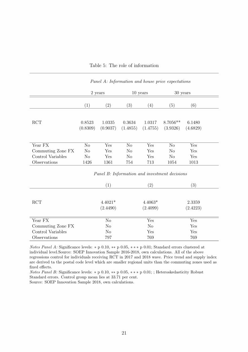
Table 5: The role of information

Panel A: Information and house price expectations

2 years 10 years 30 years

(1) (2) (3) (4) (5) (6)

RCT 0.8523 1.0335 0.3634 1.0317 8.7056** 6.1480(0.8309) (0.9037) (1.4855) (1.4755) (3.9326) (4.6829)


Panel B: Information and investment decisions

(1) (2) (3)

RCT 4.4021* 4.4063* 2.3359(2.4490) (2.4099) (2.4223)

Year FX No Yes YesCommuting Zone FX No No YesControl Variables No Yes YesObservations 797 769 769

Notes Panel A: Significance levels: ∗ p 0.10, ∗∗ p 0.05, ∗ ∗ ∗ p 0.01; Standard errors clustered atindividual level.Source: SOEP Innovation Sample 2016-2018, own calculations. All of the aboveregressions control for individuals receiving RCT in 2017 and 2018 wave. Price trend and supply indexare derived ta the postal code level which are smaller regional units than the commuting zones used asfixed effects.Notes Panel B: Significance levels: ∗ p 0.10, ∗∗ p 0.05, ∗ ∗ ∗ p 0.01; ; Heteroskedasticity RobustStandard errors. Control group mean lies at 33.71 per cent.Source: SOEP Innovation Sample 2018, own calculations.

21

ReferencesAlmenberg, J. and A. Dreber (2015): “Gender, stock market participation and

financial literacy,” Economics Letters, 137, 140–142.

Armona, L., A. Fuster, and B. Zafar (2019): “Home Price Expectations and Be-haviour: Evidence from a Randomized Information Experiment,” The Review of Eco-nomic Studies, 86, 1371–1410.

Bailey, M., C. Ruiqing, T. Kuchler, and J. Stroebel (2018): “The EconomicEffects of Social Networks: Evidence from the Housing Market,” Journal of PoliticalEconomy, 126, 2224–2276.

Bao, H. and T. Gong, C.M. Yamato (2016): “Endowment effect and housing deci-sions,” International Journal of Strategic Property Management, 5, 341–353.

BMF (2017): “Abschlussbericht, Spending Review (Zyklus 2016/2017) zum PolitikbereichWohnungswesen,” Bundesministerium der Finanzen: Spending Reviews.

Bracke, P. (2013): “How long do housing cycles last? A duration analysis for 19 OECDcountries,” Journal of Housing Economics, 22, 213–230.

Breunig, C., I. Grabova, P. Haan, F. Weinhardt, and G. Weizsäcker (2021):“Long-run expectations of households,” Journal of Behavioral and Experimental Fi-nance, 31, 100535.

Case, K. E., R. J. Schiller, and A. K. Thompson (2012): “What Have They BeenThinking? Home Buyer Behavior in Hot and Cold Markets,” NBER Working PaperSeries 18400.

Case, K. E. and R. J. Shiller (1989): “The Efficiency of the Market for Single-FamilyHomes,” The American Economic Review, 79, 125–137.

Chan, S., S. Dastrup, and I. G. Ellen (2016): “Do homeowners mark to market?a comparison of self-reported and estimated market home values during the housingboom and bust,” Real Estate Economics, 44, 627–657.

Charness, G. and U. Gneezy (2012): “Strong Evidence for Gender Differences in RiskTaking,” Journal of Economic Behavior and Organization, 83, 50–58.

Duca, J. V., J. Muellbauer, and A. Murphy (2021): “What Drives House PriceCycles? International Experience and Policy Issues,” Journal of Economic Literature,59, 773–864.

Gao, A., Z. Lin, and C. F. Na (2009): “Housing market dynamics: Evidence of meanreversion and downward rigidity,” Journal of Housing Economics, 18, 256–266.

Genovese, D. and C. Mayer (1997): “Personal Experiences and Expectations aboutAggregate Outcomes,” American Economic Review, 87, 255–269.

Glaeser, E. L. and J. Gyourko (2006): “Housing Dynamics,” Working Paper 12787,National Bureau of Economic Research.

22

Glaeser, Edward, L., J. Gyourko, E. Morales, and C. G. Nathanson (2014):“Housing dynamics: An urban approach,” Journal of Urban Economics, 81, 45–56.

Goebel, J., M. Grabka, S. Liebig, M. Kroh, D. Richter, C. Schröder, andJ. Schupp (2019): “The German Socio-Economic Panel Study (SOEP),” Jahrbücherfür Nationalökonomie und Statistik / Journal of Economics and Statistics, 239, 345–360.

Goodman, J., T. Ittner, J.B. Yamato, and K. Yokotani (1992): “The accuracyof home owners’ estimates of house value,” Journal of Housing Economics, 2, 339–357.

Green, R. K., S. Malpezzi, and S. K. Mayo (2005): “Metropolitan-specific estimatesof the price elasticity of supply of housing, and their sources,” The American EconomicReview, 95, 334–339.

Grohmann, A., L. Menkhoff, C. Merkle, and R. Schmacker (2019): “EarnMore Tomorrow: Overconfident Income Expectations and Consumer Indebtedness,”SFB Rationality and Competition, Discussion Paper No. 152.

Iacoviello, M. and S. Neri (2010): “Housing Market Spillovers: Evidence from anEstimated DSGE Model,” American Economic Journal: Macroeconomics, 2, 125–64.

Kahneman, D., J. Knetsch, and H. Richard (1990): “Experimental Tests of theEndowment Effect and the Coase Theorem,” Journal of Political Economy, 98, 1325–1348.

Kholodilin, K. A., M. Andreas, and C. Michelsen (2016): “Market Break orSimply Fake? Empirics on the Causal Effects of Rent Controls in Germany,” DIWDiscussion Paper 1584.

Kindermann, F., J. Le Blanc, M. Piazzesi, and M. Schneider (2021): “Learningabout Housing Cost: Survey Evidence from the German House Price Boom,” CEPRDiscussion Papers 16223, C.E.P.R. Discussion Papers.

Knoll, K., M. Schularick, and T. Steger (2017): “No Price Like Home: GlobalHouse Prices, 1870–2012,” American Economic Review, 107, 331–353.

Kuchler, T. and B. Zafar (2019): “Personal Experiences and Expectations aboutAggregate Outcomes,” The Journal of Finance, 74, 2491–2542.

Lamorgese, A. and D. Pellegrino (2019): “Loss aversion in housing price appraisalsamong Italian homeowners,” Banca d’Italia Working Papers.

List, J. A. (2011): “Does Market Experience Eliminate Market Anomalies? The Case ofExogenous Market Experience,” The American Economic Review, 101, 313–317.

Lusardi, A. (2008): “Household Saving Behavior: The Role of Financial Literacy, Infor-mation, and Financial Education Programs,” Working Paper 13824, National Bureauof Economic Research.

Niu, G. and A. van Soest (2014): “House Proce Expectations,” IZA Discussion Papers8536.

23

Richter, D. and J. Schupp (2015): “The SOEP Innovation Sample (SOEP IS),”Schmollers Jahrbuch: Journal of Applied Social Science Studies, 135, 389–400.

Saiz, A. (2010): “Geographic Determinants of Housing Supply,” The Quarterly Journalof Economics, 125, 1253–1296.

Seiler, M. J., V. J. Seiler, S. Traub, and D. Harrison (2008): “Regret Aversionand False Reference Points in Residential Real Estate,” Journal of Real Estate Research,30, 461–474.

Shiller, R. J. (2015): Irrational Exuberance, no. 10421 in Economics Books, PrincetonUniversity Press.

Voigtlaender, M. (2010): “Why is the German Homeownership Rate so Low?” Hous-ing Studies, 24, 355–372.

Wheaton, W. C. (1999): “Real Estate “Cycles”: Some Fundamentals,” Real EstateEconomics, 27, 209–230.

24

Appendix: Figures and Tables

Figure A.1: Real House Prices in the OECD50

7510

012

515

017

5Im

mob

ilien

Wer

tent

wic

klun

g

1940 1945 1950 1955 1960 1965 1970 1975 1980 1985 1990 1995 2000 2005 2010

Note: Graph is based on Knoll et al. (2017).

Figure A.2: Developable Land Index Berlin

Source: Corine Land Cover database 2018, photointerpretation of satellite imagery

25

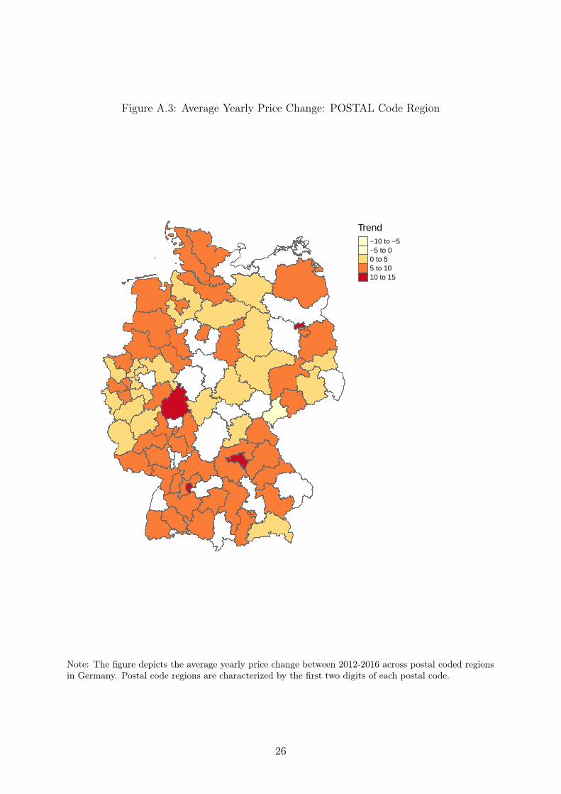
Figure A.3: Average Yearly Price Change: POSTAL Code Region

Trend−10 to −5−5 to 00 to 55 to 1010 to 15

Note: The figure depicts the average yearly price change between 2012-2016 across postal coded regionsin Germany. Postal code regions are characterized by the first two digits of each postal code.

26

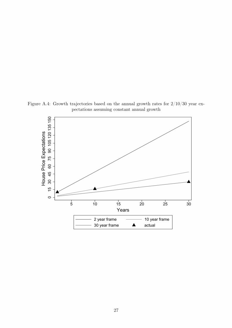
Figure A.4: Growth trajectories based on the annual growth rates for 2/10/30 year ex-pectations assuming constant annual growth

015

3045

6075

9010

512

013

515

0H

ouse

Pric

e Ex

pect

atio

ns

5 10 15 20 25 30Years

2 year frame 10 year frame30 year frame actual

27

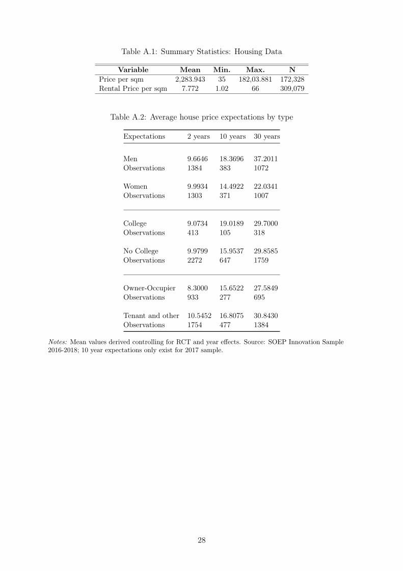
Table A.1: Summary Statistics: Housing Data

Variable Mean Min. Max. NPrice per sqm 2,283.943 35 182,03.881 172,328Rental Price per sqm 7.772 1.02 66 309,079

Table A.2: Average house price expectations by type

Expectations 2 years 10 years 30 years

Men 9.6646 18.3696 37.2011Observations 1384 383 1072

Women 9.9934 14.4922 22.0341Observations 1303 371 1007

College 9.0734 19.0189 29.7000Observations 413 105 318

No College 9.9799 15.9537 29.8585Observations 2272 647 1759

Owner-Occupier 8.3000 15.6522 27.5849Observations 933 277 695

Tenant and other 10.5452 16.8075 30.8430Observations 1754 477 1384

Notes: Mean values derived controlling for RCT and year effects. Source: SOEP Innovation Sample2016-2018; 10 year expectations only exist for 2017 sample.

28

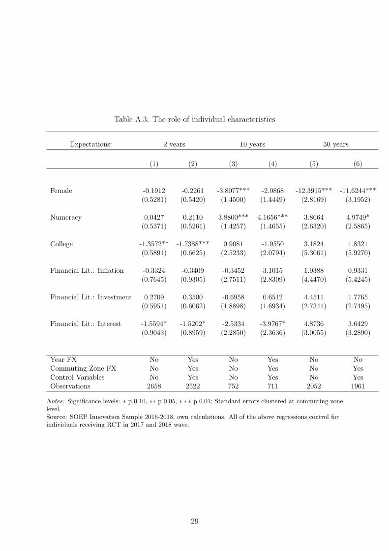
Table A.3: The role of individual characteristics


(1) (2) (3) (4) (5) (6)

Female -0.1912 -0.2261 -3.8077*** -2.0868 -12.3915*** -11.6244***(0.5281) (0.5420) (1.4500) (1.4449) (2.8169) (3.1952)

Numeracy 0.0427 0.2110 3.8800*** 4.1656*** 3.8664 4.9749*(0.5371) (0.5261) (1.4257) (1.4655) (2.6320) (2.5865)

College -1.3572** -1.7388*** 0.9081 -1.9550 3.1824 1.8321(0.5891) (0.6625) (2.5233) (2.0794) (5.3061) (5.9270)

Financial Lit.: Inflation -0.3324 -0.3409 -0.3452 3.1015 1.9388 0.9331(0.7645) (0.9305) (2.7511) (2.8309) (4.4470) (5.4245)

Financial Lit.: Investment 0.2709 0.3500 -0.6958 0.6512 4.4511 1.7765(0.5951) (0.6062) (1.8898) (1.6934) (2.7341) (2.7495)

Financial Lit.: Interest -1.5594* -1.5202* -2.5334 -3.9767* 4.8736 3.6429(0.9043) (0.8959) (2.2850) (2.3636) (3.0055) (3.2890)

Year FX No Yes No Yes No NoCommuting Zone FX No Yes No Yes No YesControl Variables No Yes No Yes No YesObservations 2658 2522 752 711 2052 1961

Notes: Significance levels: ∗ p 0.10, ∗∗ p 0.05, ∗ ∗ ∗ p 0.01; Standard errors clustered at commuting zonelevel.Source: SOEP Innovation Sample 2016-2018, own calculations. All of the above regressions control forindividuals receiving RCT in 2017 and 2018 wave.

29

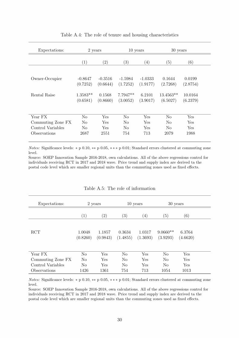
Table A.4: The role of tenure and housing characteristics


(1) (2) (3) (4) (5) (6)

Owner-Occupier -0.8647 -0.3516 -1.5984 -1.0333 0.1644 0.0199(0.7252) (0.6644) (1.7252) (1.9177) (2.7268) (2.8754)

Rental Raise 1.3583** 0.1568 7.7947** 6.2101 13.4563** 10.0164(0.6581) (0.8660) (3.0052) (3.9017) (6.5027) (6.2379)


Notes: Significance levels: ∗ p 0.10, ∗∗ p 0.05, ∗ ∗ ∗ p 0.01; Standard errors clustered at commuting zonelevel.Source: SOEP Innovation Sample 2016-2018, own calculations. All of the above regressions control forindividuals receiving RCT in 2017 and 2018 wave. Price trend and supply index are derived ta thepostal code level which are smaller regional units than the commuting zones used as fixed effects.

Table A.5: The role of information


(1) (2) (3) (4) (5) (6)

RCT 1.0048 1.1857 0.3634 1.0317 9.0660** 6.3764(0.8260) (0.9843) (1.4855) (1.3693) (3.9293) (4.6620)



30

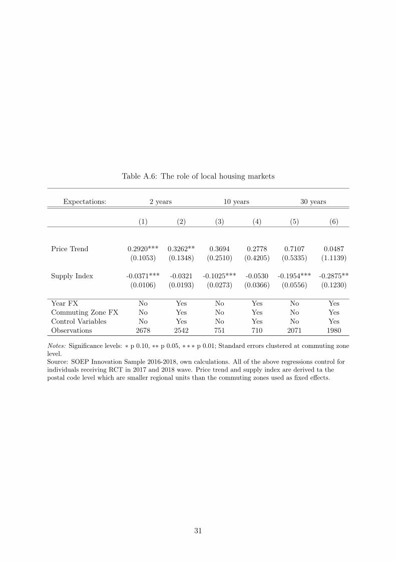
Table A.6: The role of local housing markets


(1) (2) (3) (4) (5) (6)

Price Trend 0.2920*** 0.3262** 0.3694 0.2778 0.7107 0.0487(0.1053) (0.1348) (0.2510) (0.4205) (0.5335) (1.1139)

Supply Index -0.0371*** -0.0321 -0.1025*** -0.0530 -0.1954*** -0.2875**(0.0106) (0.0193) (0.0273) (0.0366) (0.0556) (0.1230)



31

Appendix: Robustness

Clustering of standard errors In the main specification, we cluster standard errors

at the individual level, as standard errors are likely to be correlated within multiple

observations for the same individual. However, standard errors might also suffer from

heteroskedasticity at larger regional clusters. Thus, we repeat our estimations for standard

errors clustered at the commuting zone level. Tables A.3 to A.6 in the Appendix show that

the results hardly change across the different specifications and that the interpretation

remains the same. Note, however, that standard errors for the local market measures

marginally increase for the two year expectation outcome implying insignificant point

estimates when including controls and fixed effects. However, the estimate for the price

trend remains borderline significant, at the fifteen percent level with a p-value of 0.13.

Nominal vs. real expectations As described above, individuals received the fol-

lowing text when asked about their expectations: The following section focuses on your

expectations of house price developments in your area. In your opinion: How will house

prices develop in comparison to today? Participants then had the option to state whether

prices will fall, rise, remain the same, or not answering at all. Depending on their answer

individuals were asked By how much - in percent- do you think prices will fall/rise. From

this question alone it does not become clear whether individuals state their expectations

in real or in nominal terms. Therefore as a follow-up in 2019 we asked whether individuals

interpret the question in nominal or real terms. More precisely in an additional question

participants were asked:

In the previous section we asked you several questions about your expectations of house

price developments in your area. When answering the questions did you factor in general

price developments, i.e. inflation? Please be aware that it is also correct if you did not.

The majority of participants (close to 60 percent) states that they did indeed factor

in inflation whereas over 40 percent state that they did not.

32

When regressing house price expectations on an indicator whether individuals state

that they factored in inflation, we do not find a significant difference in long term and

short term expectations between both groups (see Table A.7 below).

Table A.7: Expectations and Inflation

Expectations: 2 years 30 years

(1) (2) (3) (4)

Inflation Indicator -0.0291 -0.9555 6.3316 6.8777(0.9196) (1.0781) (5.8150 ) (7.7347)

Year FX No Yes No YesCommuting Zone FX No Yes No YesControl Variables No Yes No YesObservations 619 596 445 430

Notes: Significance levels: ∗ p 0.10, ∗∗ p 0.05, ∗ ∗ ∗ p 0.01; Standard errors clustered at individual level.Source: SOEP Innovation Sample 2019, own calculations.

All in all, there is suggestive evidence that individuals appear to state their expecta-

tions in real terms, however, a relatively large proportion, i.e. approximately 40 percent,

state that they did not. Interestingly there is no significant difference in the expectations

in the short- or long-run between those who self-report that they factored in inflation

and those who did not. One potential explanation could be that individuals do not fully

grasp the concept of inflation as well as how nominal and real price developments differ.

Alternatively, individuals could expect relatively low general price appreciation, which

potentially explains why expectations between both groups do not significantly differ.

33

CENTRE FOR ECONOMIC PERFORMANCE Recent Discussion Papers

1828 Max Marczinek

Stephan Maurer Ferdinand Rauch

Trade persistence and trader identity - evidence from the demise of the Hanseatic League

1827 Laura Alfaro Cathy Bao Maggie X. Chen Junjie Hong Claudia Steinwender

Omnia Juncta in Uno: foreign powers and trademark protection in Shanghai's concession era

1826 Thomas Sampson Technology transfer in global value chains

1825 Nicholas Bloom Leonardo Iacovone Mariana Pereira-López John Van Reenen

Management and misallocation in Mexico

1824 Swati Dhingra Thomas Sampson

Expecting Brexit

1823 Gabriel M. Ahlfeldt Duncan Roth Tobias Seidel

Optimal minimum wages

1822 Fernando Borraz Felipe Carozzi Nicolás González-Pampillón Leandro Zipitría

Local retail prices, product varieties and neighborhood change

1821 Nicholas Bloom Takafumi Kawakubo Charlotte Meng Paul Mizen Rebecca Riley Tatsuro Senga John Van Reenen

Do well managed firms make better forecasts?

1820 Oriana Bandiera Nidhi Parekh Barbara Petrongolo Michelle Rao

Men are from Mars, and women too: a Bayesian meta-analysis of overconfidence experiments

1819 Olivier Chanel Alberto Prati Morgan Raux

The environmental cost of the international job market for economists

1818 Rachel Griffith John Van Reenen

Product market competition, creative destruction and innovation

1817 Felix Bracht Dennis Verhoeven

Air pollution and innovation

1816 Pedro Molina Ogeda Emanuel Ornelas Rodrigo R. Soares

Labor unions and the electoral consequences of trade liberalization

1815 Camille Terrier Parag A. Pathak Kevin Ren

From immediate acceptance to deferred acceptance: effects on school admissions and achievement in England

1814 Michael W.L. Elsby Jennifer C. Smith Jonathan Wadsworth

Population growth, immigration and labour market dynamics

1813 Charlotte Guillard Ralf Martin Pierre Mohnen Catherine Thomas Dennis Verhoeven

Efficient industrial policy for innovation: standing on the shoulders of hidden giants

1812 Andreas Teichgräber John Van Reenen

Have productivity and pay decoupled in the UK?

1811 Martin Beraja Andrew Kao David Y. Yang Noam Yuchtman

AI-tocracy

1810 Ambre Nicolle Christos Genakos Tobias Kretschmer

Strategic confusopoly evidence from the UK mobile market

The Centre for Economic Performance Publications Unit Tel: +44 (0)20 7955 7673 Email [email protected] Website: http://cep.lse.ac.uk Twitter: @CEP_LSE

mailto:[email protected]

http://cep.lse.ac.uk/

Documents

House price expectations