The Effect of Earned Versus House Money on Price Bubble Formation in Experimental Asset Markets

Review of Finance (2014) pp. 1�34doi:10.1093/rof/rfu031

The Effect of Earned Versus HouseMoney on

Price Bubble Formation in Experimental

AssetMarkets*

BRICE CORGNET1, ROBERTO HERNAN-GONZALEZ2,PRAVEEN KUJAL3 and DAVID PORTER1

1Economic Science Institute, Argyros School of Business and Economics,Chapman University, 2University of Granada, and 3Middlesex University

Abstract. Does house money exacerbate price bubbles? We compare house money assetmarket experiments with an earned money treatment where initial portfolios are constructed

from a real effort task. Bubbles occur; however, trading volumes and earnings dispersionare significantly higher with house money. We investigate the role of cognitive ability inaccounting for the differences in earnings distribution across treatments by using the cog-nitive reflection test (CRT). Low CRT subjects earned less than high CRT subjects. Low

CRT subjects were net purchasers (sellers) of shares when the price was above (below)fundamental value. The opposite was true for high CRT subjects.

JEL Classification: C92, D03, G12

1. Introduction

Do individuals make different economic decisions when they use their ownmoney (“earned money”) compared to when they do not (“house money”)?Evidence of a “house money effect” was found by Thaler and Johnson(1990) in a lottery choice experiment. They found that subjects were morelikely to exhibit risk-seeking behavior in the presence of a prior gain. Thisresult raised the question about the robustness of experimental results wheresubjects make decisions using house money.The effect of house money has been examined in bargaining and income

redistribution experiments. When money is earned, subjects tend to recog-nize merit and divide money among subjects according to their respectivecontributions (Hoffman and Spitzer, 1985; Konow, 2000; Oxoby andSpraggon, 2008). In ultimatum games when money is not earned, merit

* The authors acknowledge financial support from grant [ECO2012/00103/001] from theSpanish Ministry of Education.

� The Authors 2014. Published by Oxford University Press on behalf of the European Finance Association.

This is an Open Access article distributed under the terms of the Creative Commons Attribution Non-Commercial License

(http://creativecommons.org/licenses/by-nc/3.0/), which permits non-commercial re-use, distribution, and reproduction in any medium,

provided the original work is properly cited. For commercial re-use, please contact [email protected]

Review of Finance Advance Access published August 18, 2014 by guest on February 8, 2016

http://rof.oxfordjournals.org/D

ownloaded from

http://creativecommons.org/licenses/by-nc/3.0/

http://rof.oxfordjournals.org/

does not play a role and subjects are more likely to share the initial endow-ment equally (Guth, Schmittberger, and Schwarze, 1982; Guth and Tietz,1988).1 But Cherry, Frykblom, and Shogren (2002) show that, in a dictatorgame, 95% of the dictators follow game-theoretic predictions by nottransferring any amount to the other player when they earned theirwealth. Reinstein and Reiner (2012) obtain similar findings in a charitablegiving game. In these studies, subjects earn money prior to deciding upon theallocation of the outcome by answering a quiz (Cherry, Frykblom, andShogren, 2002; Oxoby and Spraggon, 2008), playing a simple hash markgame (Hoffman and Spitzer, 1985), adding numbers (Reinstein andReiner, 2012), or stuffing and folding envelopes (Konow, 2000). On theother hand, Cherry, Kroll, and Shogren (2005) find no evidence of thehouse money effect in voluntary contribution games. The variability ofresults across different games suggests that the effect may also be specificto the environment being tested.Even though most of the previously mentioned research provides evidence

of a house money effect in bargaining games, it is not clear how these resultsextend to market games of exchange.

HOUSE MONEY VERSUS EARNED MONEY IN ASSET MARKETS

It is well known that prices in experimental asset markets do not follow thetheoretical prediction and bubbles are commonly observed with inexperi-enced subjects (Smith, Suchanek, and Williams, 1988). Experimental assetmarkets are characterized by persistent (average) price deviation from fun-damental value in early periods, with prices significantly above fundamentalas the market progresses and then a crash to fundamental value at the end.The question we address is whether the use of house money to endow initialportfolios of cash and shares to subjects encourages the “mispricing” foundin experimental asset markets.Specifically, we investigate whether traders behave differently when they

earn their starting endowment (“Earned Money treatment”) than when theydo not (“House Money baseline”) in experimental asset markets with pricebubbles and crashes. Asset market bubbles have been found to be robust totreatments variations such as short selling, capacity to buy on margin,brokerage fees, limit price change rules (King et al., 1993; Porter andSmith, 1994) and assets generating certain dividends (Porter and Smith,

1 Note that despite extensive evidence of an effect of earned money on the allocation ofjoint outcomes, Rutstrom and Williams (2000) report no significant differences in alloca-tions whether endowments were earned or randomly generated.

2 B. CORGNET ETAL.

by guest on February 8, 2016http://rof.oxfordjournals.org/

Dow

nloaded from


1995). Further, even though the introduction of futures markets may reducebubble amplitude, it does not affect their duration (Porter and Smith, 1995).Nevertheless, a complete set of futures (one for each of the fifteen periods)seems to eliminate bubbles (Noussair and Tucker, 2006). Interestingly,bubbles tend to disappear with twice-experienced subjects even whenexperienced and inexperienced traders are mixed (Dufwenberg, Lindqvist,and Moore, 2005). However, bubbles may still be observed among twice-experienced traders when the market environment is modified by increasingliquidity and dividend uncertainty (Hussam, Porter, and Smith, 2008). Theexistence of bubbles has been partly ascribed to subjects’ irrational behaviors(Lei, Noussair, and Plott, 2001). The authors find evidence of systematicerrors in decision making accompanying bubbles. Traders engage in unprof-itable transactions at prices above the maximum possible or below theminimum possible dividend stream.The asset market environment is a good candidate to study the house

money effect as it is characterized by systematic deviations of marketprices from fundamental values in contradiction to the equilibrium predic-tions obtained in market-clearing models (Tirole, 1982). In that context, wemay wonder whether the house money effect can account for part of thediscrepancy between the fundamental value of the asset and the pricesobserved in the laboratory. Earlier research on the house money effectoffers little guidance to our current study as it mostly examines bargaininggames and aims at studying the role of house money on distributive prefer-ences. Market experiments differ considerably from these settings as they donot involve concerns for distributive preferences. The only work that con-templates the potential effect of house money in a market environment wasconducted by Ang, Diavatopoulos, Schwarz (2010). The authors conductedexperimental asset markets (as a robustness check) in which subjects playedwith their own money. No significant differences were found between thehouse money and the own money cases. Besides natural concerns with apossible selection bias, the authors’ results should be interpreted withcaution as they conducted only two experimental sessions with subjects’own money. This small sample follows from the fact that the primary goalof the authors was to assess the emergence of bubbles under different com-pensation schemes, wealth and supply constraints, as well as the effect of therelative risk aversion of traders rather than studying the house money effectper se.In order to study the effect of earned money in experimental asset

markets, we recruited subjects for a two-part experiment. In the first part,subjects had to perform a 2 hour real effort task that consisted in developinga database for a research institute. All subjects earned the same amount in

EARNEDMONEYANDBUBBLES 3


Dow

nloaded from


this part and were told that their money was carried over for the experimentwhich will be realized in the second part.2 In the second part, which tookplace after 3 days, subjects participated in a standard experimental assetmarket with certain dividends (Smith, Suchanek, and Williams, 1988;Porter and Smith, 1995). The value of each subject’s initial portfoliocomposed of both cash and shares was exactly equal to the fixed paymentearned from the first-day task ($31.5).3

Our main findings are that bubbles were similar in the house and earnedmoney treatments. However, relative to the house money treatment, trans-action volumes were 31% lower in the earned money treatment. One of thedirect effects of reduced transactions is that the dispersion of earnings wasmore pronounced in the house money compared with earned money treat-ment. We investigate earnings dispersion further by categorizing subjectsaccording to their performance on the cognitive reflection test (CRT)(Frederick, 2005).4 We find that subjects with low CRT scores were netpurchasers (sellers) of shares when the price was above (below) fundamentalvalue while the opposite was true for subjects with high CRT scores. As aresult, high CRT subjects earned more money on average than the initialvalue of their portfolio while low CRT subjects earned less. This result wastrue for both the house and earned money treatments.

2. Experimental Design and Hypothesis

2.1 PROCEDURE

One hundred and eighty subjects from a major university participated in thehouse money (henceforth HM) and earned money (henceforth EM)treatments.

2.1.a The HM treatment

In the baseline HM treatment, subjects only participated in the asset marketexperiment for which they were endowed with a portfolio of cash and sharesworth $31.50 from the experimenter (house money). The HM experimentswere conducted as standard asset market experiments (Smith, Suchanek, andWilliams, 1988). Nine subjects each participated in a fifteen period asset

2 Further, we made no promises in terms of a safety net that subjects would be able to

recover the money from the experiment (as in Clark (2002)).3 In addition, subjects were paid a $10 show-up fee for each appearance.4 This 3-min questionnaire was administered while subjects waited for their payments at theend of the experiment. As is common in this literature, the CRT was not incentivized.

4 B. CORGNET ETAL.


Dow

nloaded from


market. Our only departure from the standard structure was that thedividend was certain (Porter and Smith, 1995). This was dictated by thedesign requirement of the EM treatment where we wanted to ensure thatsubjects did not see their earned money being put to risk. A certain dividendguaranteed that if the subjects simply held on to their shares and cash en-dowment they would finish the market experiment with the amount ofmoney they had previously earned.

2.1.b The EM treatment

Subjects in the EM treatment were told that they will be participating in anexperiment that has two parts (Table I) with the second part taking place 3days after the first part. Subjects were told that they will be performing atask related to a database for a research institute in the first part and that theamount earned in the task, $31.50, will be carried over to the second part.5

They were also informed that they would be paid in cash for the entireexperiment at the end of the second part. Including the 2-day show-upfees subjects earned, on average, $51.50.6 As a result, in the EM treatmentfinal earnings were partially coming from show-up fees which were notearned by subjects. The show-up fee, however, could not be used fortrading and, as such, differed from the endowment subjects receive instandard experimental asset markets. In that respect, our treatment is oneof earned endowment. We did not have subjects earn their show-up feesbecause the IRB rules at the laboratory where the studies were conductedrequire that subjects cannot be recruited without being paid a show-up fee(or their show-up fee being put at risk).7

In the first part of the experiment, subjects performed a task requiring(real) effort of 2 h. The task performed by the subjects was intended toresemble as closely as possible a short-term job.8 We ensured that subjectswere aware of the economic significance of their work task by explicitlystating in the instructions that the database to be developed was going tobe used by a research institute (which was indeed the case). In order to stress

5 See Appendix B for instructions.6 The show-up fee was $10 each day. A high show-up fee was used in this treatment toensure that subjects who participated in the first day experiment would come back for the

second. This was indeed the case for all subjects but one.7 In addition, recruiting subjects who would accept to earn their show-up fees may createselection effects possibly attracting a high proportion of risk lovers and overconfident

subjects.8 This task is similar to that in Falk and Ichino (2006) where recruited students foldedpapers and stuffed envelopes to prepare the mailing of a questionnaire study for theUniversity of Zurich.



Dow

nloaded from


the difference between a standard laboratory experiment and the work task(in the EM treatment), we conducted the two parts, that is the work task andthe experimental asset market, on two separate days.9

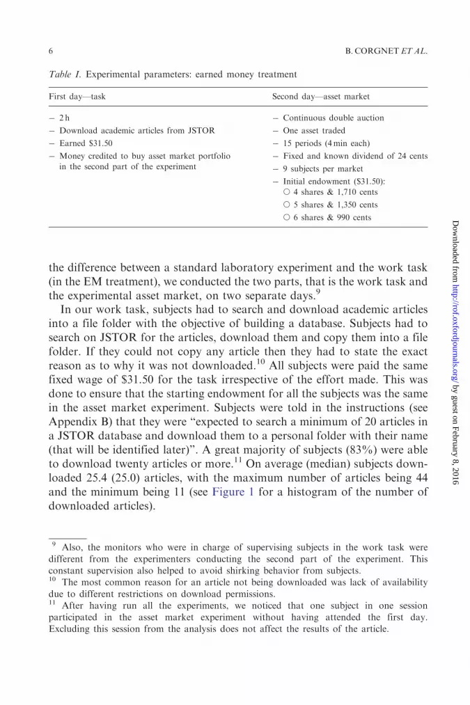
In our work task, subjects had to search and download academic articlesinto a file folder with the objective of building a database. Subjects had tosearch on JSTOR for the articles, download them and copy them into a filefolder. If they could not copy any article then they had to state the exactreason as to why it was not downloaded.10 All subjects were paid the samefixed wage of $31.50 for the task irrespective of the effort made. This wasdone to ensure that the starting endowment for all the subjects was the samein the asset market experiment. Subjects were told in the instructions (seeAppendix B) that they were “expected to search a minimum of 20 articles ina JSTOR database and download them to a personal folder with their name(that will be identified later)”. A great majority of subjects (83%) were ableto download twenty articles or more.11 On average (median) subjects down-loaded 25.4 (25.0) articles, with the maximum number of articles being 44and the minimum being 11 (see Figure 1 for a histogram of the number ofdownloaded articles).

Table I. Experimental parameters: earned money treatment

First day—task Second day—asset market

� 2 h

� Download academic articles from JSTOR

� Earned $31.50

� Money credited to buy asset market portfolio

in the second part of the experiment

� Continuous double auction

� One asset traded

� 15 periods (4min each)

� Fixed and known dividend of 24 cents

� 9 subjects per market

� Initial endowment ($31.50):

� 4 shares & 1,710 cents

� 5 shares & 1,350 cents

� 6 shares & 990 cents

9 Also, the monitors who were in charge of supervising subjects in the work task were

different from the experimenters conducting the second part of the experiment. Thisconstant supervision also helped to avoid shirking behavior from subjects.10 The most common reason for an article not being downloaded was lack of availability

due to different restrictions on download permissions.11 After having run all the experiments, we noticed that one subject in one sessionparticipated in the asset market experiment without having attended the first day.Excluding this session from the analysis does not affect the results of the article.

6 B. CORGNET ETAL.


Dow

nloaded from


In the second part, the subjects participated in an asset market experiment(Table I). Each experiment had nine subjects. Each asset earned a fixeddividend of 24 cents in each period and lasted for fifteen periods. Subjectsstarted the experiment with four, five, or six shares and had cash endow-ments of 1,710, 1,350, or 990 cents, respectively. The total value of the en-dowment equaled $31.50 dollars for all subjects, which is exactly equal to themoney they earned in the prior task. Subjects were told several times thattheir earnings will be used in the asset market experiment. For example,subjects were informed explicitly that:

(i) Before participating in this experiment, you earned $31.50 by workingon the database for the research institute during 2 hours. This fullamount of cash will be used to pay for your initial portfolio in thecurrent experiment.

We provided each subject with detailed calculations regarding the value oftheir initial portfolio which was composed of both cash and shares (seeInstructions page 3 in Appendix C). We then clarified the link between thework task completed in the first part of the experiment and the initial port-folio endowment.

(ii) Notice that the value of your initial portfolio corresponds to theearnings in the 2 hours you spent working on the database.

Point (ii) was further repeated in the experimental summary at the end ofthe instructions where subjects were told that the initial value of their port-folio ($31.50) corresponded to the earnings they obtained in the work task 3days ago. This was done to ensure that the subjects knew that they were

Figure 1. Histogram of number of downloaded articles.



Dow

nloaded from


playing with the amount they earned in the earlier task. We summarize ourexperimental design in Table II.

2.1.c CRT

To complement our analysis of the effect of earned money on individualbehavior, we collected data regarding subjects’ cognitive ability at the end ofeach experimental session. We used the CRT as a measure of cognitiveability (Frederick, 2005). The CRT has been found to correlate withgeneral measures of intelligence as well as different aspects of individualdecision making such as risk and time preferences (Frederick, 2005;Oechssler, Roider, and Schmitz, 2009) and levels of reasoning (Branas-Garza, Garcıa-Munoz, and Hernan-Gonzalez, 2012). The CRT consists ofthe following three questions:

(1) A bat and a ball cost $1.10 in total. The bat costs $1.00 more than theball. How much does the ball cost?

(2) If it takes five machines 5 min to make five widgets, how long would ittake 100 machines to make 100 widgets?

(3) In a lake, there is a patch of lily pads. Every day, the patch doubles insize. If it takes 48 days for the patch to cover the entire lake, how longwould it take for the patch to cover half of the lake?

The CRT score corresponds to the total number of correct answers andvaries from 0 to 3.

2.2 HYPOTHESIS

Bubbles in experimental asset markets are characterized in many dimensionssuch as price deviations from fundamental value, duration, and tradevolume. If house money has an effect it will be manifested in changes inthese measures. It seems natural to suppose (and as suggested by Thaler andJohnson, 1990) that subjects might engage in greater speculative behaviorwhen they have none of their own money at stake and that this speculative

Table II. Experimental design

Treatment

Number of subjects

per sessions

Number of

sessions

House Money Baseline 9 10

Earned Money Treatment 9 10

8 B. CORGNET ETAL.


Dow

nloaded from


behavior will likely result in higher trading volumes and mispricing. If, asLei, Noussair, and Plott (2001) and Kirchler, Huber, and Stuockl (2012)suggest, bubbles are a manifestation of some underlying confusion aboutthe market environment, then earned money should have no effect. Giventhis, we examine the following null hypothesis in our experiments.

Hypothesis: Earned money will have no effect on the characteristics of pricebubbles.

3. Results

We use different measures of bubbles considered in the literature in order tocheck for differences between treatments and also to compare with resultsreported by other authors. We consider the following measures of bubbles:12

(1) Amplitude: measures the trough-to-peak change in asset value relativeto its fundamental value. This is measured as, A¼Max{Pt�ft

E : t¼1 . . . 15}�Min{Pt�ft

E : t¼ 1 . . . 15}. Where, Pt is the average marketprice in period t, ft is the fundamental value of the asset in period t,and E is the expected dividend value over the life of the asset.

(2) Duration: measures the length, in periods, in which there is an observedincrease in market prices relative to the fundamental value of the asset.Formally, duration is defined as:

D ¼Maxfm: Pt�ft < Ptþ1 � ftþ1 < . . . < Ptþm � ftþmg:

(3) Haessel-R2 (Walter W. Haessel, 1978): measures goodness-of-fitbetween observed (mean prices) and fundamental values. It is appro-priate, since the fundamental values are exogenously given. Haessel-R2

tends to 1 as trading prices tend to fundamental values.

(4) Normalized average price deviation (NAV): sums up the absolute de-viation between the average price and the fundamental value for eachof the fifteen periods. It is defined as follows:

NAV ¼X15t¼1

jPt � ftj

15:

(5) Normalized absolute price deviation (NAP): as defined in Haruvy andNoussair (2006), NAP measures the per-share aggregate overvaluation

12 See Dufwenberg, Lindqvist, and Moore (2005) and Corgnet, Kujal, and Porter (2010).



Dow

nloaded from


(or undervaluation), relative to the fundamental value of the asset in agiven period and is defined as:

NAP ¼XK

k¼1

jPk � fkj

100� 45;

where, Pk is the price of the k-th transaction in the experiment, 45 thetotal number of shares, 100 is a normalization scalar, and fk is thefundamental value of the asset when the k-th transaction takes place.Large values of NAP reflect volumetric deviations from fundamentals.This measure is similar to the normalized average price deviation.However, NAV does not depend on the number of trades and canthen be used to compare the extent of mispricing in sessions with dif-ferent levels of trading volumes.

(6) Turnover: measures the volume of share transactions relative to thenumber of shares on issue in the market:

Turnover ¼

XT

t¼1qt

45;

where, T is the number of trading periods, qt is the number of trans-actions in period t and 45 is the total number of shares in the marketwhich in our case is equal to 45.

3.1 BUBBLE CHARACTERISTICS

In Figure 2, we plot per period median price for each session in the HMtreatment. Interestingly, although prices always start below the fundamentalvalue, in three of our sessions average prices keep close to the fundamentalvalue for most of the periods. Table III reports bubble measures for eachsession.We confirm the results of Porter and Smith (1995) by not identifying

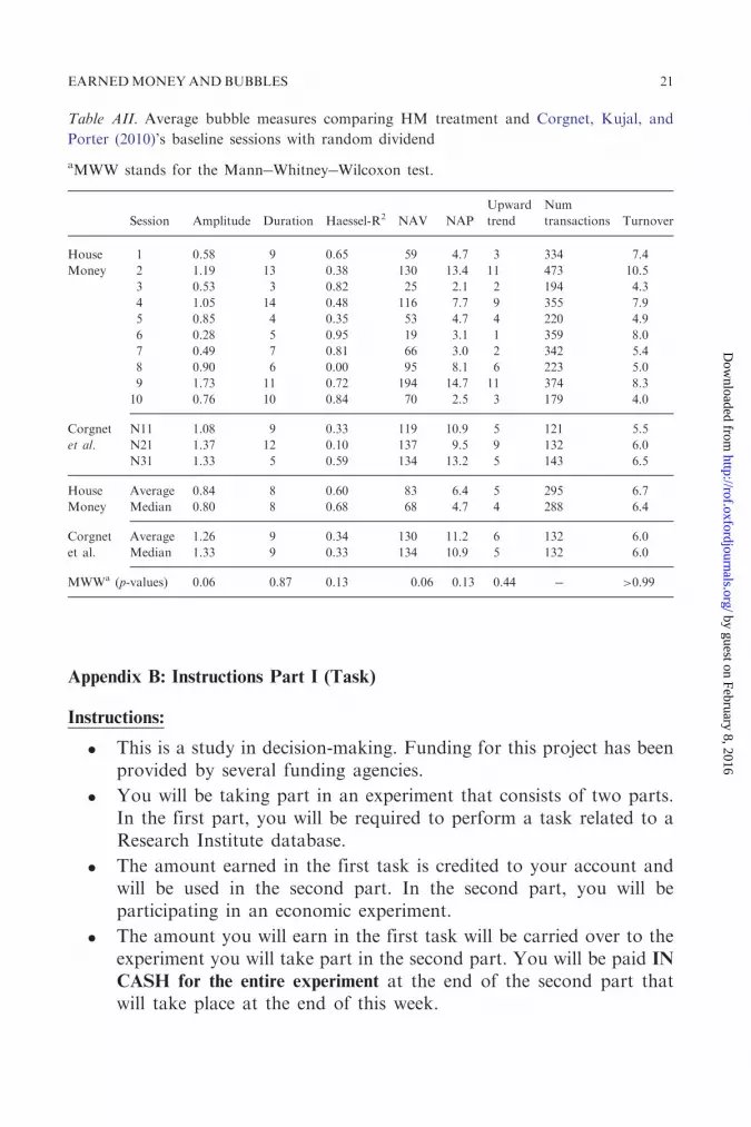
significant differences in bubble measures when comparing experimentalasset markets with certain dividends versus markets with asset marketswith uncertain dividends.13 We perform a comparison of different bubblemeasures for treatments with randomly drawn dividends and inexperiencedsubjects against our HM experiments (see Table AI in Appendix A). We find

13 We compare our results (with certain dividends) with the results of Corgnet, Kujal, andPorter (2010) (uncertain dividends).

10 B. CORGNET ETAL.


Dow

nloaded from


that bubble measures do not differ significantly from those obtained in theHM treatment when considering standard significance levels.14

Figure 3 shows per-period median price for the EM treatment. Thoughdiffering in magnitudes, bubbles form in 6 out of 10 cases in the HM treat-ment and in 5 out of 10 cases in the EM treatment. From Figures 2 and 3,one can see significant mispricing in both the house money and the EMtreatments. We reject the equality of all bubbles measures between theHM and EM treatments using a multivariate test (p¼ 0.38).15

Looking at each bubble measure separately (Table III), we observe nosignificant differences between the house money and the EM treatmentexcept for NAP (p¼ 0.01) and turnover (p¼ 0.07). A lower NAP tells usthat relative to the HM experiments, and considering all transactions, pricesin the EM treatment were closer to the fundamental value. Average tradingvolumes are 31% lower in the EM treatment compared with the HM treat-ment. Note that NAP is, by definition, closely linked to trading volumes.

Figure 2. Period median prices in the House Money treatment.

14 We use a multivariate test comparing all bubble measures in our study and in Corgnet,Kujal, and Porter (2010). We report a p-value of 0.21. When comparing each bubblemeasure separately (see Table A2 in Appendix A), we report marginally significant differ-

ences for amplitude and NAP between our house money treatment and the baseline treat-ment in Corgnet, Kujal, and Porter (2010).15 We used command sr.loc.test in R to do these spatial rank tests of multivariate location.We obtained similar values using a Hotelling’s T2 test (p¼ 0.41).



Dow

nloaded from


NAP automatically increases with an increase in the number of transactionsK as long as transactions are completed at prices that are not exactly equal tofundamental values. The fact that the measures of mispricing that are notaffected by trading volumes, such as NAV and Haessel-R2 values, do notdiffer across treatments suggests that there are no significant differences inthe pattern of prices across treatments. We conclude that the difference inthe NAP measure across treatments is mostly driven by differences in tradingvolumes. We summarize our findings as follows.

Result 1: We find that the earned money treatment has no significant effecton asset mispricing, but has a significant effect on measures of tradingvolume.

Table III. Average bubble measures for different treatments

aMann�Whitney�Wilcoxon test.

Treatment Session Amplitude Duration Haessel-R2 NAV NAP Turnover

House money

1 0.58 9 0.65 59 4.7 7.4

2 1.19 13 0.38 130 13.4 10.5

3 0.53 3 0.82 25 2.1 4.3

4 1.05 14 0.48 116 7.7 7.9

5 0.85 4 0.35 53 4.7 4.9

6 0.28 5 0.95 19 3.1 7.98

7 0.49 7 0.81 66 3.0 5.38

8 0.90 6 0.00 95 8.1 4.96

9 1.73 11 0.72 194 14.7 8.31

10 0.76 10 0.84 70 2.5 3.98

Earned Money

1 0.46 6 0.82 29 1.5 3.0

2 0.60 4 0.80 37 1.3 2.9

3 0.84 5 0.53 69 1.8 3.0

4 0.52 8 0.92 81 2.8 2.5

5 0.74 4 0.61 27 2.0 5.8

6 1.13 12 0.69 116 9.2 8.8

7 0.53 7 0.79 40 3.3 5.2

8 0.24 2 0.97 12 1.0 4.8

9 0.39 7 0.84 37 2.7 5.5

10 0.56 5 0.88 29 2.1 4.0

House MoneyAverage 0.84 8 0.60 83 6.4 6.7

Median 0.80 8 0.68 68 4.7 6.4

Earned MoneyAverage 0.60 6 0.78 48 2.8 4. 6

Median 0.55 6 0.81 37 2.1 4.4

MWWa (p-values) 0.13 0.21 0.13 0.13 0.01 0.07

12 B. CORGNET ETAL.


Dow

nloaded from


Finally, we investigate the distribution of subjects’ earnings across treat-ments. Figure 4 below shows a histogram of subjects’ earnings at the end ofthe experiment for each treatment.16

We observe that the dispersion of earnings, measured by their standarddeviation and the Gini coefficient, is significantly greater in the HM treatmentthan in the EM treatment (Table IV). Note that a crucial element in explainingdifferences in earnings dispersion across treatments is the difference in tradingvolumes (K) between the earned money and the HM treatment.17

Figure 3. Period median prices in the Earned Money treatment.

16 We obtain a positive but not significant correlation between subject’s performance in thetask (number of articles downloaded) and either their CRT score (Spearman’s r¼ 0.1013,

p¼ 0.36) or their earnings in the asset market experiment (Spearman’s r¼ 0.1087, p¼ 0.31).We also ran a regression of the number of articles downloaded controlling for subjects’earnings and CRT score (or a dummy that takes value 1 for positive CRT scores, and zerootherwise) and found that all the coefficients were not significantly different from zero (all

p’s> 0.38).17 The variance of earnings increases in K. Indeed, let us consider a market with twotraders, each of them being endowed with the same amount of cash C. Let us call B the

number of times trader 1 is buying the asset while S is the total number of times trader 1 isselling the asset. The variance of earnings can then be expressed as follows: Var½Cþ

PBb¼1

ðfb � PbÞ þPS

s¼1ðPs � fsÞ� where fbðfsÞ is the fundamental value of the asset when trader 1

buys (sells) the asset for the bth(sth) times. Also, PbðPsÞ is the price of the asset when trader 1buys (sells) the asset for the bth(sth) times. Assuming that prices are independent and iden-tically distributed random variables with variance s2 then the variance of earnings is:(Bþ S)s2¼Ks2.



Dow

nloaded from


Interestingly, we find that earnings dispersion by session, measured by thestandard error of subject’s earnings, is highly correlated with trading volumes(Spearman’s r¼ 0.697, p¼ 0.03 and r¼ 0.746, p¼ 0.01 for the HM and EMtreatments, respectively).18

Our findings regarding earnings dispersion are summarized as follows.

Result 2: Compared with the house money treatment, earnings dispersion issignificantly lower in the earned money treatment.

In the next section, we examine the correlation between CRT scores andindividual trader behavior.

3.2 CRT CORRELATES

The CRT scores provide one, among other possible, measures of subjects’cognitive skills (Frederick, 2005) which can be used to sort subjects accord-ingly. Table V provides subject score (0, 1, 2, 3) on the CRT and its rela-tionship with subjects’ earnings across treatments.In Table V, we compare earnings for subjects with a CRT score of zero

with earnings for subjects with scores greater than zero (last column).19 With

Figure 4. Histogram of subjects’ earnings by treatment.

18 Similar values are found using Gini coefficients instead of standard deviations ofsubjects’ earnings (Spearman’s r¼ 0.649, p¼ 0.04 and r¼ 0.709, p¼ 0.02 for the HM and

EM treatments, respectively).19 The same procedure has been used in Branas-Garza, Garcıa-Munoz, and Hernan-Gonzalez (2012). Our results are stronger if we compare the tails of the CRT scores dis-tribution (subjects with 0 and 3 scores only).

14 B. CORGNET ETAL.


Dow

nloaded from


house money, subjects with a CRT score of zero earn on average $22.31,which is 40% less than the subjects who have positive CRT scores ($37.08,MWW, p¼ 0.0012). This result also holds for the treatment with earnedmoney (MWW, p¼ 0.0021). However, this difference in earnings acrosssubjects with different CRT scores is lower when subjects use their ownmoney (EM treatment). In particular, the earnings of subjects with a CRTscore of zero were 12% larger in the EM treatment compared with the HMtreatment while the earnings of subjects with a positive CRT score were 9%lower (MWW, p¼ 0.5692 and p¼ 0.4553, respectively). In addition, subjectswith a CRT score of three earned 120.9% more than those with a score ofzero in the HM treatment (MWW, p< 0.001), whereas the difference inearnings between these subjects was only equal to 40.4% in the EM treat-ment (MWW, p< 0.001).

Table IV. Subjects’ final earnings

aMann�Whitney�Wilcoxon test.

Treatment Session Standard error Gini coefficient

House Money

1 28.64 0.45

2 32.61 0.53

3 20.55 0.34

4 17.88 0.30

5 21.68 0.36

6 26.73 0.41

7 13.24 0.20

8 14.59 0.25

9 23.26 0.39

10 12.56 0.21

Earned Money

1 14.90 0.23

2 11.37 0.19

3 7.04 0.10

4 7.91 0.13

5 15.44 0.24

6 24.34 0.39

7 23.55 0.39

8 9.03 0.15

9 17.79 0.27

10 18.71 0.30

House MoneyAverage 21.17 0.35

Median 21.11 0.35

Earned MoneyAverage 15.01 0.24

Median 15.17 0.23

MWWa (p-values) 0.08 0.05



Dow

nloaded from


In Figure 5, we show subjects’ average portfolio value at the end of eachperiod by CRT score. From the very beginning, subjects with a higher CRTscore earn more money and this difference increases over time. Interestingly,HM subjects earning differences across CRT scores are even larger. UnderEM, subjects with a higher CRT score cannot take full advantage of subjectswith low scores.20

We summarize our results regarding CRT scores and earnings as follows.

Result 3: Subjects with positive CRT scores earn significantly more thansubjects with a zero CRT score. Differences in earnings across subjectswith different CRT scores are significantly more pronounced in the housemoney treatment than in the earned money treatment.

This result is in line with the recent work of Cueva and Rustichini (2012)according to which subjects with high cognitive skills measured with non-verbal IQ tend to outperform subjects with low cognitive skills.

Table V. Baseline treatment—mean (median) earnings

[Number of observations].

aMann�Whitney�Wilcoxon test. This test reports the comparison of subjects’ earnings withCRT¼ 0 and subjects with CRT> 0.

CRT 0 1 2 3 >0

MWWa

(p-values)

House Money $ 22.31 $ 35.71 $ 30.45 $ 49.29 $ 37.08 0.0012

($ 22.12) ($ 35.21) ($ 32.33) ($ 40.75) ($ 35.57)

[34] [24] [19] [13] [56]

Earned Money $ 25.07 $ 33.53 $ 31.98 $ 35.19 $ 33.71 0.0021

($23.49) ($ 34.88) ($ 31.64) ($ 35.83) ($ 34.34)

[23] [27] [17] [23] [67]

20 For each treatment, we ran a panel data regression, with random effects and clusters bysession, of subjects’ portfolio value on a dummy variable capturing CRT scores (CRTd which

takes value one if the subject’s CRT is positive and value zero otherwise), period dummies,and the interaction effect. The portfolio value of subjects with positive CRT scores is signifi-cantly higher than those subjects with zero CRT scores. Interestingly, in the HM treatment

the difference in the portfolio value increases over time, as the coefficients of the perioddummies (with respect to the first period, omitted) are negative and decrease over time forsubjects with zero CRT score, while they are positive and increase over time for subjects with

positive CRT score (the coefficients of all the fifteen interaction terms, CRTd�Period, are

significant, all p’s< 0.095). In the EM treatment, however, the difference in portfolio value byCRT remains constant across periods (no period dummy is significant, and the coefficients ofall the fifteen interaction terms are not significant either, all p’s> 0.143).

16 B. CORGNET ETAL.


Dow

nloaded from


Now, we study trading patterns in more detail to uncover some of thepossible reasons for the observed differences in subjects’ earnings. In par-ticular, we study whether subjects were net buyers or net sellers of the assetwhen the price was lower or higher than the fundamental value of the asset.We compute the number of net purchases per period as the number of pur-chases minus the number of sales of an individual for that period. Table VIpresents the results of a panel data, with random effects and clusters bysession, of the net number of purchases on a dummy variable capturingCRT scores (CRTd) and on the difference between the average period

price and the fundamental value relative to the fundamental value (Pt�FVt

FVt).

We show that subjects with a CRT score of zero are net buyers (sellers) whenthe asset price is above (below) the fundamental value since the coefficient

associated with the variable (Pt�FVt

FVt) is positive and significant. Note that this

result is statistically significant for the HM treatment, whereas it is onlymarginally so in the EM treatment. Subjects with a CRT score greaterthan zero are net buyers (sellers) when the asset price is below (above) thefundamental value since the coefficient associated with the variable

[ðPt�FVt

FVtÞ þ CRTd

� ðPt�FVt

FVtÞ] is negative and significant. This finding is

particularly interesting as it shows that high CRT subjects may be feedingthe bubble in the early stages of the experiment and get out of it before itcrashes. Further, the effect of CRT score on net purchases is morepronounced in the HM treatment than in the EM treatment.

Figure 5. Portfolio value at the end of each period.



Dow

nloaded from


Our findings regarding trading patterns across subjects with differentCRT scores are summarized as follows:21

Result 4: Subjects with positive CRT scores buy (sell) shares when the assetprice is below (above) the fundamental value. Subjects with a zero CRTscore behave in the opposite manner.

This result means that in our asset market experiments, which is a zero-sum game, there is a transfer of earnings from subjects with low CRT scoresto subjects with high CRT scores. High CRT subjects purchase shares inthe early periods, when prices are below the fundamental value and sellthose shares when the prices exceed the fundamental value (see left panelof Figure 6). This transfer of wealth is less pronounced in the EM treatment(see right panel of Figure 6).

Table VI. Subjects’ number of net purchases by period

CRTd¼ 0 if subject’s CRT¼ 0 and 1 otherwise. Pt is the (session) average price of period t.

FVt is the fundamental value of period t.

*p< 0.10, **p< 0.05, and ***p< 0.01.

Variables House Money Earned Money

Constant 0.0689 �0.1282*

CRTd�0.1001 0.1716*

Pt�FVt

FVt0.0765** 0.0689*

CRTd� Pt�FVt

FVt

� ��0.1358** �0.1144**

R2 0.0053 0.0021

Wald chi2 9.02** 7.04*

Pt�FVt

FVt

� �þ CRTd

� Pt�FVt

FVt

� ��0.0593** �0.0455**

21 We also studied differences in the total number of transactions for all treatments (and

number of transactions by treatment across periods) by CRT score and did not find anysignificant differences (MWW, p¼ 0.923 and p¼ 0.410 in treatment HM and EM, respect-ively). This result holds across periods (MWW, most p’s> 0.164 for all periods and treat-ments, except for period 8 in the Earned Money treatment, p¼ 0.074).

18 B. CORGNET ETAL.


Dow

nloaded from


4. Conclusion

In this article, we have studied the house money effect in an experimentalasset market with bubbles and crashes. We found that even though bubblesstill occurred in the EM treatment, trading volumes were significantlyreduced. The reduction in trading volumes implied a significant decreasein the dispersion of subjects’ earnings in the EM treatment compared withhouse money.We investigated earnings dispersion by categorizing subjects according to

their cognitive ability which was measured using the CRT. We found thatsubjects with lower CRT scores were net purchasers (sellers) of shares whenthe price was above (below) fundamental value while the opposite was truefor subjects with higher CRT scores. Consequently, high CRT subjectsearned more money on average than the initial value of their portfoliowhile low CRT subjects earned less. This result was true for both thehouse and EM treatments.Our main conclusion is that there is indeed a house money effect in ex-

perimental asset markets. The house money effect manifests itself in tradingvolume that subsequently affects earnings dispersion. Bubbles, however, aremaintained and we find no differences between our two treatments, orcomparing our results with other experiments with uncertain dividends.We take a preliminary step by studying individual behavior in assetmarkets as reflected by the well-known CRT. We use the CRT to sortsubject behavior in asset markets and find that cognitive abilities, as reflected

Figure 6. Average number of shares held at the end of the period by CRT score and acrossperiods for house money (on the left panel) and for earned money (on the right panel).



Dow

nloaded from


by the CRT, do seem to matter. Individuals with a high CRT score feed thebubble in the early stages and get out of it in later periods. Further researchneeds to be done to better understand the link between cognitive abilities andbubble formation in experimental asset markets.Our findings also shed light on the ongoing discussion regarding excessive

trading in financial markets where average mutual-fund turnover hasincreased from 15% in the 1950s to around 100% in 2011 (Edelen, Evans,and Kadlec, 2013). This excessive trading which could be explained by in-vestors’ overconfidence and urge to “do something” (Dow and Gorton,1997; Odean, 1999) could be tamed by redesigning incentive packages offund managers. For example, a proportion of their base salary could beautomatically invested in their clients’ portfolio.

Appendix A: Comparison with other studies

Bubble measures in our HM treatment and those reported by Corgnet et al.(2010) are not significantly different when using a multivariate test(p¼ 0.21).22

Table AI. Average bubble measures for related studiesa

aAll of them are studies with the same number of periods (15) and traders (9). Dataobtained from Corgnet, Kujal, and Porter (2010).

Amplitude Duration NAV NAP

House Money 0.84 8.2 6.4 82.7

Corgnet, Kujal, and Porter (2010) 1.26 10.3 11.2 130

Smith, Van Boening, and Wellford (2000) 1.39 � 5.5 �Porter and Smith (1995) 1.53 10.1 � �King et al. (1993) 1.61 9.5 11.8 �Smith, Suchanek, and Williams (1988) 1.24 10.2 5.7 �

22 We used command sr.loc.test in R to do these spatial rank tests of multivariate location.We obtained similar values using a Hotelling’s T2 test (p¼ 0.21).

20 B. CORGNET ETAL.


Dow

nloaded from


Appendix B: Instructions Part I (Task)

Instructions:

. This is a study in decision-making. Funding for this project has beenprovided by several funding agencies.

. You will be taking part in an experiment that consists of two parts.In the first part, you will be required to perform a task related to aResearch Institute database.

. The amount earned in the first task is credited to your account andwill be used in the second part. In the second part, you will beparticipating in an economic experiment.

. The amount you will earn in the first task will be carried over to theexperiment you will take part in the second part. You will be paid IN

CASH for the entire experiment at the end of the second part thatwill take place at the end of this week.

Table AII. Average bubble measures comparing HM treatment and Corgnet, Kujal, and

Porter (2010)’s baseline sessions with random dividend

aMWW stands for the Mann�Whitney�Wilcoxon test.

Session Amplitude Duration Haessel-R2 NAV NAP

Upward

trend

Num

transactions Turnover

House

Money

1 0.58 9 0.65 59 4.7 3 334 7.4

2 1.19 13 0.38 130 13.4 11 473 10.5

3 0.53 3 0.82 25 2.1 2 194 4.3

4 1.05 14 0.48 116 7.7 9 355 7.9

5 0.85 4 0.35 53 4.7 4 220 4.9

6 0.28 5 0.95 19 3.1 1 359 8.0

7 0.49 7 0.81 66 3.0 2 342 5.4

8 0.90 6 0.00 95 8.1 6 223 5.0

9 1.73 11 0.72 194 14.7 11 374 8.3

10 0.76 10 0.84 70 2.5 3 179 4.0

Corgnet

et al.

N11 1.08 9 0.33 119 10.9 5 121 5.5

N21 1.37 12 0.10 137 9.5 9 132 6.0

N31 1.33 5 0.59 134 13.2 5 143 6.5

House

Money

Average 0.84 8 0.60 83 6.4 5 295 6.7

Median 0.80 8 0.68 68 4.7 4 288 6.4

Corgnet

et al.

Average 1.26 9 0.34 130 11.2 6 132 6.0

Median 1.33 9 0.33 134 10.9 5 132 6.0

MWWa (p-values) 0.06 0.87 0.13 0.06 0.13 0.44 � >0.99



Dow

nloaded from


Today’s Task:

. In this part you will be performing a task for a Research Institutedatabase.. You have a list of academic articles on your desk.

. You are expected to search a minimum of 20 articles in a JSTORdatabase and download them to a folder (that will be identifiedlater).

. You will be credited $31.50 for this task.

Where to save the articles?

. Please, right click on the mouse and create a new folder on thedesktop.

. Please, name the folder now using your own complete name.

. You will be saving the articles into this folder.

How to save an article?

. For example, the article:� Edward L. Glaeser, David I. Laibson, Jose A. Scheinkman,

Christine L. Soutter, 2000, Measuring Trust, The QuarterlyJournal of Economics, 115, 811�846.

. Go to, http://www.jstor.org/

. Then select Economics.

. Type in the name of the journal, e.g., “Quarterly Journal ofEconomics”

. Go to the corresponding year and page numbers

. Click on the article and save it to your folder.

How do I download the article from JSTOR?

. Once you find the article you will find a screen similar to the onebelow

22 B. CORGNET ETAL.


Dow

nloaded from

http://www.jstor.org/


� click on View pdf on the right hand side.

. Then click on proceed to pdf.

. Then right-click on the article to save as in your folder in the formatmentioned earlier.



Dow

nloaded from


Format of the saved article

Author1&Author2_TitleofPaper_JournalInitialsYear.pdf

. For example, the article:� Edward L. Glaeser, David I. Laibson, Jose A. Scheinkman,

Christine L. Soutter, 2000, Measuring Trust, The QuarterlyJournal of Economics, 115, 811�846.

. Will be saved as, Glaeser&Laibson&Scheinkman&Soutter_Measur-ing Trust_ QJE2000.pdf

. Note: Journal initials are the first letters of the journal title.� For example, for Quarterly Journal of Economics the initials are

QJE, for Economic Journal the initials are EJ, for AmericanEconomic Review the initials are AER etc . . .

What if you do not find the article on JSTOR?

. Move on to the next article on the list.

. Please state on the handout that the article was not available.

24 B. CORGNET ETAL.


Dow

nloaded from


What if the journal is not available on JSTOR?

. State on the handout that the journal is not available on JSTOR andmove on to the next article on your list.

. Please make sure that all articles are saved using the naming formatwe provide above.

Appendix C: Instructions Part II (Asset Markets)

INSTRUCTIONS (1/14)

This is an experiment in market decision making. You will be paid in cashfor your participation at the end of the experiment. Different participantsmay earn different amounts. What you earn depends on your decisions andthe decisions of others.[(Only EM treatment) Before participating in this experiment, you

earned $31.50 by working on the ESI database during 2 hours. This full

amount of cash will be used to pay for your initial portfolio in the current

experiment.]

The experiment will take place through computer terminals at which youare seated. If you have any questions during the instruction round, raise yourhand and a monitor will come by to answer your question. If any difficultiesarise after the experiment has begun, raise your hand, and someone willassist you.

INSTRUCTIONS (2/14)

In this experiment you will be able to buy and sell a commodity, calledShares, from one another.At the start of the experiment, every participant will be given some Cash

and Shares.The shares last for EXACTLY 15 periods of trading. After each

trading period the share will earn a dividend of 24 cents. Thus, if you hada share at the end of period 1, you would get a return of 24 cents for thatperiod.If you held a share from period 1 until the end of period 15, then

that share would return to you a total of $3.60 (15� 24 cents) over the15 periods. Similarly, if you bought a share in period 2 and held it fromperiod 2 until the 15th period, the accumulated dividends would be $3.36

(14� 24 cents).



Dow

nloaded from


INSTRUCTIONS (3/14)23

You will start the experiment with six shares and 990 cents in cash. Theinitial value of your portfolio is identical and equal to $31.50. This is the casebecause the total dividend value of each share over the 15 periods is equal to$3.60 (15� 24 cents):

990 centsþ 6� $3:60 ¼ 31:50:

[(Only EM treatment) Notice that the value of your initial portfolio corresponds

to the earnings in the 2 hours you spent working on the ESI database.]

INSTRUCTIONS (4/14)

During every period, traders can buy or sell shares from one another bymaking offers to buy or to sell.Every time a trade is made, it will be shown as a dark GREEN dot in the

graph located on the left of the lower part of your screen. Transactions arealso listed on theMarket Book located on the right of the graph. If you buy ashare (or somebody sold it to you), the cell in the Market Book will be shownin light BLUE. The cell will be shown in RED if you sell a share (orsomebody buys it from you). The cells that are shown without colorscorrespond to transactions in which you are not involved either as a buyeror as a seller.

Figure C1. Lower part of your trading screen (graph and market book).

23 This part of the instructions was specific to each subject’s initial portfolio. The initialendowment of cash and number of shares were 990, 1,350, or 1,710 cents and 6, 5, or 4shares, respectively.

26 B. CORGNET ETAL.


Dow

nloaded from


INSTRUCTIONS (5/14)

To enter a new order to buy or to sell a share, type in the price at which youwould like to buy, or sell, in the appropriate Add order to Buy box or Addorder to Sell box. Click the Add order to Buy or Add order to Sell button tosubmit your order.

INSTRUCTIONS (6/14)

Every time someone posts an order to buy a share, it will be added to the listof best orders to buy (in the BLUE quadrant). This list shows only the bestFOUR orders. Every time someone makes an offer to sell a share, it will be

Figure C2. Upper part of your screen (Buy and Sell).



Dow

nloaded from


added to the list of the best orders to sell (in the RED quadrant). This listshows only the best FOUR orders.The orders to buy will be listed from the highest price to the lowest price,

while the orders to sell will be listed from the lowest price to the highest price.Your own orders in this list will be highlighted in ORANGE. For example,

you have just posted an order to sell at a price equal to 202 and this cor-responds to the third best order in the market (that is, the third lowest order tosell). This order will appear in the third place in the list of orders to sell.

INSTRUCTIONS (7/14)

To accept an existing order from another participant, click the Buy a share ator Sell at share at buttons located on the right of the list of orders to sell andorders to buy, respectively. The list of orders to buy shows you the fourhighest orders to buy that are currently available on the market, while the listof orders to sell shows you the four lowest orders to sell. By clicking on theBuy a share at button, you buy at the listed price of 104 in the currentexample; by clicking on the Sell at share at button, you sell at the listedprice of 96 in the current example. Your own existing orders to buy or sellare highlighted in ORANGE.In the situation illustrated in the following screen shot, the best order to

sell corresponds to a price of 104 (the lowest value in the list of orders tosell). This is the price at which you can currently buy the share. The bestorder to buy corresponds to a price of 96 (the highest value in the list oforders to buy since this is the only order to buy currently available). This isthe price at which you can currently sell the share.

Figure C3. Upper part of your screen (Orders to buy and to sell).

28 B. CORGNET ETAL.


Dow

nloaded from


INSTRUCTIONS (8/14)

Whenever you enter new orders to buy, or sell, you will have those orderslisted in a table below the list of orders to buy and sell. By double clicking onany cell in the table, you can cancel your own orders.

INSTRUCTIONS (9/14)

At the end of every period, each share will pay a dividend of 24 cents. Thedividend for each period will appear in the Dividends Table.The earned dividends (for shares) of each period will be added to the cash

account of the holder.The number of your shares will change, only when you buy, or sell, shares.Notice that you cannot place orders to buy for an amount that is greater

than your current Cash. The information regarding the remaining cashavailable to buy is displayed in the box below your current Cash. Also,you cannot place more orders to sell shares than the Number of shares youcurrently hold. The information regarding the remaining shares available tosell is displayed below your current Number of shares.

Figure C4. Upper part of your screen (Orders to buy and to sell).



Dow

nloaded from


INSTRUCTIONS (10/14)

During a period and each time you place an order or complete a transactiona message will appear in the box above the dividends table. This message boxprovides indications on whether your order or transaction has beencompleted successfully. For example, if you attempt to buy a share at aprice that is higher than your current cash holdings, a message will appearin the box stating that you do not have sufficient cash to buy this share.

30 B. CORGNET ETAL.


Dow

nloaded from



An example:

Suppose you have 5 shares and 150 in Cash at the start of a period, andyou make one transaction during the period purchasing a share for 110cents within the period, and the dividend for the period is 24 cents, then:Your Cash holdings will increase by 34 cents (Dividends of 24 times 6shares minus a purchase at 110). Your new cash holding will thus be150þ 34¼ 184 cents.

Your share holdings will increase from 5 to 6 units.



Dow

nloaded from



Another example:At the end of the previous period, you had 4 shares and 242 in Cash.Suppose in the next period you make two transactions. You sell one

share for 130 and another share for 110, and the dividend for the period is24, then:Your Cash holdings will increase by 288 cents (Dividends of 24 times 2

shares plus sales of 130 plus 110). Your new cash holding will thus be242þ 288¼ 530 cents.Your share holdings will, however, decrease from 4 to 2 units.


This experiment will last for 15 periods. Each period will last for severalminutes. The remaining time (in seconds) will appear on the top of yourscreen.

When the time is about to expire, the color will change to RED.

We will have a short practice period to allow you to become familiar withentering orders and making trades.

INSTRUCTIONS SUMMARY (14/14)

(1) You will be given an initial amount of Cash and Shares.

(2) Every share generates a dividend of 24 cents at the end of each of 15trading periods.

(3) You can submit orders to BUY shares and orders to SELL shares.

(4) You make trades by buying at the current lowest order to sell or sellingat the current highest order to buy.

(5) The market lasts for 15 periods. At the end of period 15, there will beone last dividend draw. After that the share expires and is worthnothing to you.

32 B. CORGNET ETAL.


Dow

nloaded from


(6) The initial value of your portfolio is equal to $31.50 (¼990 centsþ 6shares� $3.60).24 [(Only EM treatment) This amount corresponds to the

earnings you obtained in the 2 hours you spent working on the ESI

database.]

Click “Ready” to start the experiment.

References

Ang, J. S., Diavatopoulos, D., and Schwarz, T. V. (2010) The creation and control of

speculative bubbles in a laboratory setting, in: C.-F. Lee, A. Lee, and J. Lee (eds),

Handbook of Quantitative Finance and Risk Management, Springer US, 137�164.Branas-Garza, P., Garcıa-Munoz, T., and Hernan-Gonzalez, R. (2012) Cognitive effort in

the beauty contest game, Journal of Economic Behavior & Organization 83, 254�260.Cherry, T. L., Frykblom, L. P., and Shogren, J. F. (2002) Hardnose the dictator, American

Economic Review 92, 1218�1221.Cherry, T. L., Kroll, S., and Shogren, J. F. (2005) The impact of endowment heterogeneity

and origin on public good contributions: evidence from the lab, Journal of Economic

Behavior & Organization 57, 357�365.Clark, J. (2002) House money effects in public good experiments, Experimental Economics

5, 223�231.Corgnet, B., Kujal, P., and Porter, D. (2010) The effect of reliability, content and timing of

public announcements on asset trading behavior, Journal of Economic Behavior &

Organization 76, 254�266.Cueva, C. and Rustichini, A. (2012) Financial market instability: myths and truths.

Working paper.Dow, J. and Gorton, G. (1997) Noise trading, delegated portfolio management, and

economic welfare, Journal of Political Economy 105, 1024�1050.Dufwenberg, M., Lindqvist, T., and Moore, E. (2005) Bubbles and experience: an experi-

ment on speculation, American Economic Review 95, 1732�1737.Edelen, R., Evans, R., and Kadlec, G. (2013) Shedding light on ‘invisible’ costs: trading

costs and mutual fund performance, Financial Analysts Journal 69, 34�44.Falk, A. and Ichino, A. (2006) Clean evidence of peer effects, Journal of Labor Economics

24, 39�58.Frederick, S. (2005) Cognitive reflection and decision making, Journal of Economic

Perspectives 19, 25�42.Guth, W., Schmittberger, R., and Schwarze, B. (1982) An experimental analysis of ultima-

tum bargaining, Journal of Economic Behavior & Organization 3, 367�388.Guth, W. and Tietz, R. (1988) Ultimatum bargaining for a shrinking cake: an experimental

analysis, in: R. Tietz, W. Albers, and R. Selten (eds), Bounded Rational Behavior in

Experimental Games and Markets, Springer, Berlin.Haessel, W. W. (1978) Measuring goodness of fit in linear and nonlinear models, Southern

Economic Journal 44, 648�652.Haruvy, E. and Noussair, C. N. (2006) The effect of short selling on bubbles and crashes in

experimental spot asset markets, Journal of Finance 61, 1119�1157.

24 Again, this paragraph was specific to each subject’s initial portfolio.



Dow

nloaded from


Hoffman, E. and Spitzer, M. (1985) Entitlements, rights, and fairness: an experimental

examination of subjects’ concepts of distributive justice, Journal of Legal Studies 14,

259�297.Hussam, R. N., Porter, D., and Smith, V. L. (2008) Thar she blows: can bubbles be

rekindled with experienced subjects?, American Economic Review 98, 924�937.King, R. R., Smith, V. L., Williams, A. W., and Van Boening, M. (1993) The robustness of

bubbles and crashes in experimental stock markets, in: R. Day and P. Chen (eds), Nonlinear

Dynamics and Evolutionary Economics, Oxford University Press, Oxford, pp. 183�200.Kirchler, M., Huber, J., and Stuockl, T. (2012) Thar she bursts � Reducing confusion

reduces bubbles, American Economic Review 102, 865�883.Konow, J. (2000) Fair shares: accountability and cognitive dissonance in allocation deci-

sions, American Economic Review 90, 1072�1092.Lei, V., Noussair, C. N., and Plott, C. R. (2001) Nonspeculative bubbles in experimental

asset markets: lack of common knowledge of rationality vs. actual irrationality,

Econometrica 69, 831�859.Noussair, C. N. and Tucker, S. (2006) Futures markets and bubble formation in experi-

mental asset markets, Pacific Economic Review 11, 167�184.Odean, T. (1999) Do investors trade too much?, American Economic Review 89, 1279�1298.Oechssler, J., Roider, A., and Schmitz, P. W. (2009) Cognitive abilities and behavioral

biases, Journal of Economic Behavior & Organization 72, 147�152.Oxoby, R. J. and Spraggon, J. (2008) Mine and yours, property rights in dictator games,

Journal of Economic Behavior & Organization 65, 703�713.Porter, D. P. and Smith, V. L. (1994) Stock market bubbles in the laboratory, Applied

Mathematical Finance 1, 111�128.Porter, D. P. and Smith, V. L. (1995) Futures contracting and dividend uncertainty in

experimental asset markets, The Journal of Business 68, 509�541.Reinstein, D. and Riener, H. (2012) Decomposing desert and tangibility effects in a char-

itable giving experiment, Experimental Economics 15, 229�240.Rutstrom, E. E. and Williams, M. B. (2000) Entitlements and fairness, an experimental

study of distributive preferences, Journal of Economic Behavior & Organization 43, 75�89.Smith, V. L., Suchanek, G. L., and Williams, A. W. (1988) Bubbles, crashes, and endogen-

ous expectations in experimental spot asset markets, Econometrica 56, 1119�1151.Smith, V. L., van Boening, M. V., and Wellford, C. P. (2000) Dividend timing and behavior

in laboratory asset markets, Economic Theory 16, 567�583.Thaler, R. H. and Johnson, E. J. (1990) Gambling with the house money and trying to

break even: the effects of prior outcomes on risky choice, Management Science 36, 643�660.Tirole, J. (1982) On the possibility of speculation under rational expectations, Econometrica

50, 1163�1182.

34 B. CORGNET ETAL.


Dow

nloaded from


Documents

The Effect of Earned Versus House Money on Price Bubble Formation in Experimental Asset Markets