Bank of Canada Banque du Canada

Working Paper 2002-30 / Document de travail 2002-30

Inflation Expectations and Learningabout Monetary Policy

by

David Andolfatto, Scott Hendry, and Kevin Moran

ISSN 1192-5434

Printed in Canada on recycled paper

Bank of Canada Working Paper 2002-30

October 2002

Inflation Expectations and Learningabout Monetary Policy

by

David Andolfatto, 1 Scott Hendry, 2 and Kevin Moran 2

1Department of EconomicsSimon Fraser University

Burnaby, British Columbia, Canada V5A 1S6dandolfa@sfu.ca

2Monetary and Financial Analysis DepartmentBank of Canada

Ottawa, Ontario, Canada K1A 0G9shendry@bankofcanada.cakmoran@bankofcanada.ca

The views expressed in this paper are those of the authors.No responsibility for them should be attributed to the Bank of Canada.

iii

Contents

Acknowledgements. . . . . . . . . . . . . . . . . . . . . . . . . . . . . . . . . . . . . . . . . . . . . . . . . . . . . . . . . . . . ivAbstract/Résumé. . . . . . . . . . . . . . . . . . . . . . . . . . . . . . . . . . . . . . . . . . . . . . . . . . . . . . . . . . . . . . . v

1. Introduction . . . . . . . . . . . . . . . . . . . . . . . . . . . . . . . . . . . . . . . . . . . . . . . . . . . . . . . . . . . . . . 1

2. Empirical Evidence of Inflation Expectations . . . . . . . . . . . . . . . . . . . . . . . . . . . . . . . . . . . . 3

3. The Model . . . . . . . . . . . . . . . . . . . . . . . . . . . . . . . . . . . . . . . . . . . . . . . . . . . . . . . . . . . . . . . 5

3.1 Households . . . . . . . . . . . . . . . . . . . . . . . . . . . . . . . . . . . . . . . . . . . . . . . . . . . . . . . . . . 5

3.2 Firms . . . . . . . . . . . . . . . . . . . . . . . . . . . . . . . . . . . . . . . . . . . . . . . . . . . . . . . . . . . . . . . 6

3.3 Financial intermediaries . . . . . . . . . . . . . . . . . . . . . . . . . . . . . . . . . . . . . . . . . . . . . . . . 7

3.4 Equilibrium . . . . . . . . . . . . . . . . . . . . . . . . . . . . . . . . . . . . . . . . . . . . . . . . . . . . . . . . . . 7

4. Monetary Policy. . . . . . . . . . . . . . . . . . . . . . . . . . . . . . . . . . . . . . . . . . . . . . . . . . . . . . . . . . . 7

4.1 The monetary policy rule . . . . . . . . . . . . . . . . . . . . . . . . . . . . . . . . . . . . . . . . . . . . . . . 7

4.2 Monetary policy shocks and monetary policy shifts. . . . . . . . . . . . . . . . . . . . . . . . . . . 8

4.3 Incomplete information and learning . . . . . . . . . . . . . . . . . . . . . . . . . . . . . . . . . . . . . . 9

5. Calibration and Solution of the Model. . . . . . . . . . . . . . . . . . . . . . . . . . . . . . . . . . . . . . . . . 12

5.1 Preferences and technology . . . . . . . . . . . . . . . . . . . . . . . . . . . . . . . . . . . . . . . . . . . . 12

5.2 Parameters of the interest-rate-targeting rule . . . . . . . . . . . . . . . . . . . . . . . . . . . . . . . 13

5.3 Shifts and shocks to monetary policy . . . . . . . . . . . . . . . . . . . . . . . . . . . . . . . . . . . . . 13

6. Monte Carlo Simulation of the Model . . . . . . . . . . . . . . . . . . . . . . . . . . . . . . . . . . . . . . . . . 15

6.1 Impulse responses following a regime shift . . . . . . . . . . . . . . . . . . . . . . . . . . . . . . . . 15

6.2 The experiment . . . . . . . . . . . . . . . . . . . . . . . . . . . . . . . . . . . . . . . . . . . . . . . . . . . . . . 16

6.3 Results for the benchmark case. . . . . . . . . . . . . . . . . . . . . . . . . . . . . . . . . . . . . . . . . . 17

6.4 Sensitivity analysis . . . . . . . . . . . . . . . . . . . . . . . . . . . . . . . . . . . . . . . . . . . . . . . . . . . 18

7. Conclusion . . . . . . . . . . . . . . . . . . . . . . . . . . . . . . . . . . . . . . . . . . . . . . . . . . . . . . . . . . . . . . 20

References. . . . . . . . . . . . . . . . . . . . . . . . . . . . . . . . . . . . . . . . . . . . . . . . . . . . . . . . . . . . . . . . . . . 22

Tables . . . . . . . . . . . . . . . . . . . . . . . . . . . . . . . . . . . . . . . . . . . . . . . . . . . . . . . . . . . . . . . . . . . . . . 25

Figures. . . . . . . . . . . . . . . . . . . . . . . . . . . . . . . . . . . . . . . . . . . . . . . . . . . . . . . . . . . . . . . . . . . . . . 27

Appendix A: Kalman Filter . . . . . . . . . . . . . . . . . . . . . . . . . . . . . . . . . . . . . . . . . . . . . . . . . . . . . 34

iv

Acknowledgements

The authors wish to acknowledge the expert research assistance of Veronika Dolar. We thank

Walter Engert, Paul Gomme, Andrew Levin, Césaire Meh, and seminar participants at the Bank of

Canada, the 2002 CEA meeting, and the 2002 North American Summer Meeting of the

Econometric Society for useful comments and discussions.

v

tion.

etimes

odel,

that

ents

ion

on

uch

e

in

e

les

me une

ral

s. Le

des

ue

s

Abstract

Various measures indicate that inflation expectations evolve sluggishly relative to actual infla

In addition, they often fail conventional tests of unbiasedness. These observations are som

interpreted as evidence against rational expectations.

The authors embed, within a standard monetary dynamic stochastic general-equilibrium m

an information friction and a learning mechanism regarding the interest-rate-targeting rule

monetary policy authorities follow. The learning mechanism enables optimizing economic ag

to distinguish between transitory shocks to the policy rule and occasional shifts in the inflat

target of monetary policy authorities.

The model’s simulated data are consistent with the empirical evidence. When the informati

friction is activated, simulated inflation expectations fail conventional unbiasedness tests m

more frequently than in the complete-information case when this friction is shut down. Thes

results suggest that an important size distortion may occur when conventional tests of

unbiasedness are applied to relatively small samples dominated by a few significant shifts

monetary policy and sluggish learning about those shifts.

JEL classification: E47, E52, E58Bank classification: Business fluctuations and cycles; Economic models

Résumé

Divers indicateurs donnent à penser que les attentes d’inflation évoluent plus lentement qu

l’inflation observée. En outre, dans bien des cas, ils se révèlent entachés de biais lorsqu’on

soumet aux tests usuels d’absence de biais. Le rejet de ces tests est parfois interprété com

réfutation de l’hypothèse de rationalité des attentes.

Les auteurs intègrent, dans un modèle monétaire stochastique dynamique d’équilibre géné

standard, un élément de friction relatif à l’acquisition de l’information et un mécanisme

d’apprentissage concernant la règle de taux d’intérêt qu’appliquent les autorités monétaire

mécanisme d’apprentissage permet aux agents économiques ayant un comportement

d’optimisation de distinguer les chocs temporaires que subit la règle de politique monétaire

modifications apportées à l’occasion à la cible d’inflation poursuivie.

Les données simulées dans le modèle sont conformes aux observations empiriques. Lorsq

l’élément de friction est pris en compte, les attentes d’inflation simulées comportent un biai

vi

le

nt

rs.

d’après les tests standard, et ce, beaucoup plus souvent que dans le cas d’une information

complète, sans friction. Ces résultats indiquent qu’une forte distorsion de niveau est possib

lorsque les tests standard d’absence de biais sont appliqués à des échantillons relativeme

restreints caractérisés par seulement quelques changements d’orientation importants de la

politique monétaire et que les agents mettent beaucoup de temps à reconnaître ces dernie

Classification JEL : E47, E52, E58Classification de la Banque : Cycles et fluctuations économiques; Modèles économiques

1

1. Introduction

Various measures indicate that inflation expectations evolve sluggishly relative toactual inflation. Expectations tend to underpredict inflation during periods of risinginflation and overpredict it during periods of diminishing inflation.1 Related to thissluggishness phenomenon is the stylized fact, documented by an extensive empiricalliterature, that measured inflation expectations often reject the hypotheses of unbi-asedness and efficiency.2 These results have sometimes been interpreted as evidenceagainst rational behaviour on the part of economic agents.

This paper assesses whether an information friction over, and a learning mech-anism about, the interest-rate-targeting rule followed by monetary policy authori-ties, once embedded in a standard monetary dynamic stochastic general-equilibrium(DSGE) model, can lead simulated data to quantitatively replicate the empirical ev-idence against the unbiasedness of inflation expectations.

The following information friction is introduced. We assume that the interest-rate-targeting rule followed by monetary policy authorities is affected by transitoryshocks but also, occasionally, by persistent shifts in the inflation target that anchorsthe rule. We interpret the transitory shocks in the standard way, as instances ofmonetary policy authorities wishing to deviate from their rule for a short period; forexample, to react to financial shocks. We assume that the occasional shifts in theinflation target reflect changes in economic thinking about the optimal inflation rate,or the appointment of a new central bank head with different preferences for inflationoutcomes. Importantly, we also assume that these transitory shocks and persistentshifts cannot be separately observed (nor credibly revealed). Consequently, marketparticipants must solve a signal-extraction problem to distinguish between the twocomponents, giving rise to a learning rule that shares some features with adaptive-expectations processes.3

Next, we calibrate the parameters of this signal-extraction problem and embedit within the limited-participation environment developed by Christiano and Gust(1999). We then repeatedly simulate the model and perform unbiasedness tests onthe artificial data equivalent to those performed on measured inflation expectations.

Our simulations identify substantially different outcomes in the unbiasednesstests when the information friction is active compared with the complete-informationcase when it is shut down. Specifically, the fraction of rejections when complete in-formation is assumed never deviates significantly from the level suggested by the

1For example, Dotsey and DeVaro (1995) uncover economic agents’ expectations about U.S.inflation—using commodity futures data—over the disinflationary episode of 1980Q1–1983Q3, andfind that expected inflation exceeded actual inflation in all but three periods for the eight-monthforecasts and in each period for the one-year forecasts. DeLong (1997) reports that, during theU.S. inflationary episode of the 1970s, a consensus, private sector inflation forecast underestimatedthe actual inflation rate in every year and that, remarkably, in each and every year inflation wasactually expected to fall (Figure 6.9, 267).

2See Thomas (1999), Roberts (1997), and Croushore (1997), and the references they cite.3Muth (1960) demonstrates that the optimal learning rule in such a signal-extraction problem

resembles adaptive-expectation processes.

2

size of the tests. In contrast, when the information friction is activated, the testsreject the null hypothesis of unbiasedness much more frequently—between two tofives times—although our model embodies the “rational expectations” solution con-cept by construction. Interestingly, these differences are much attenuated when thesample size of each simulation is increased significantly.

Given these results, we propose the following interpretation of the empiricalrejections of the unbiasedness hypothesis. The process by which economic agentsform inflation expectations may be fundamentally sound, but a few significant shiftsin monetary policy, coupled with relatively sluggish learning about those shifts, canlead to significant size distortions of the tests. Furthermore, while this effect maybe sufficient to trigger excessive rejections of the null hypothesis in small samples,it should disappear as the sample size grows.

Environments with information frictions and learning effects similar to the one wedescribe have been used previously, notably to rationalize the persistent responsesof real variables following monetary policy shocks.4 Our paper makes a twofoldcontribution to this literature.

First, we locate the signal-extraction problem within an interest-rate-targetingrule, rather than a monetary-growth process. This feature, which our model shareswith that of Erceg and Levin (2001), allows the learning literature to connect withthe now-standard view of the proper modelling of monetary policy.

Second, we evaluate the incomplete information and learning framework not byits capacity to generate persistence in the dynamics of real variables, as Erceg andLevin (2001) do, but by its ability to replicate the dynamic relationship that existsbetween realized and expected inflation. More precisely, we specify parameter valuesfor the underlying components of the monetary policy process and verify whetherthe rejection of the unbiasedness hypothesis emerges as an implication of these pa-rameter values. Conversely, Erceg and Levin (2001) choose parameter values tomatch the relationship between realized and expected inflation and concentrate onthe implication of their chosen specification for real variables. Our analysis com-plements theirs and broadens the scrutiny of the empirical relevance of incompleteinformation and learning effects.

Our strategy is similar to that of Kozicki and Tinsley (2001a), who argue that thefrequent empirical rejections of the term structure’s expectation hypothesis couldbe the result of economic agents learning only gradually about shifts in the FederalReserve’s objectives. Kozicki and Tinsley embed a learning mechanism similar toours in a simple macroeconomic environment and assess whether the expectationhypothesis is rejected by the simulated data. In earlier contributions, Lewis (1988,1989) uses similar intuition to verify whether sluggish learning can generate the

4Recent contributions include Andolfatto and Gomme (1999), Moran (1999), Andolfatto,Hendry, and Moran (2000), Erceg and Levin (2001), who analyze closed economies, and Sill andWrase (1999), who study an open-economy environment. In an early contribution using a differentmodelling technology, but appealing to very similar ideas, Brunner, Cukierman, and Meltzer (1980)analyze the properties of a stochastic IS–LM model in which agents cannot distinguish betweenpermanent and transitory shocks to real and nominal variables.

3

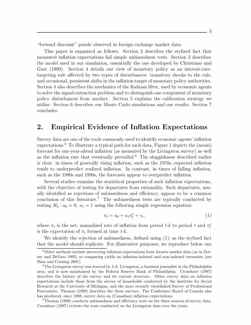
“forward discount” puzzle observed in foreign exchange market data.

This paper is organized as follows. Section 2 describes the stylized fact thatmeasured inflation expectations fail simple unbiasedness tests. Section 3 describesthe model used in our simulation, essentially the one developed by Christiano andGust (1999). Section 4 details our view of monetary policy as an interest-rate-targeting rule affected by two types of disturbances: transitory shocks to the rule,and occasional, persistent shifts in the inflation target of monetary policy authorities.Section 4 also describes the mechanics of the Kalman filter, used by economic agentsto solve the signal-extraction problem and to distinguish one component of monetarypolicy disturbances from another. Section 5 explains the calibration strategy weutilize. Section 6 describes our Monte Carlo simulations and our results. Section 7concludes.

2. Empirical Evidence of Inflation Expectations

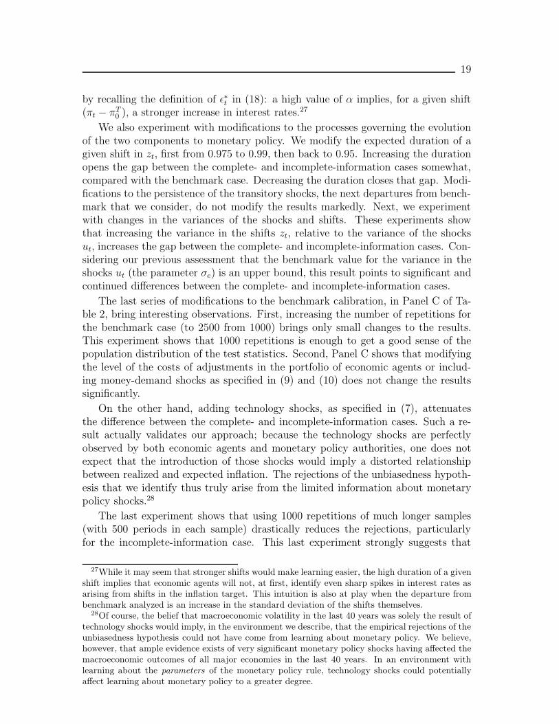
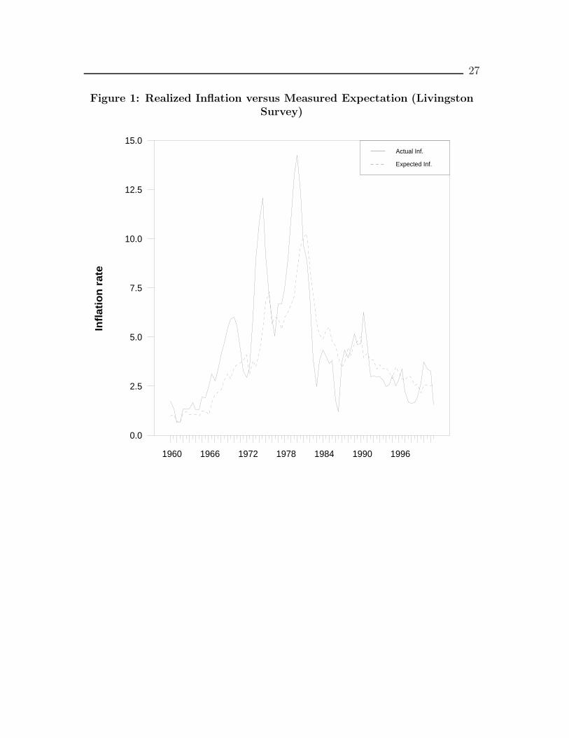
Survey data are one of the tools commonly used to identify economic agents’ inflationexpectations.5 To illustrate a typical path for such data, Figure 1 depicts the (mean)forecast for one-year-ahead inflation (as measured by the Livingston survey) as wellas the inflation rate that eventually prevailed.6 The sluggishness described earlieris clear: in times of generally rising inflation, such as the 1970s, expected inflationtends to underpredict realized inflation. In contrast, in times of falling inflation,such as the 1980s and 1990s, the forecasts appear to overpredict inflation.

Several studies examine the statistical properties of such inflation expectations,with the objective of testing for departures from rationality. Such departures, usu-ally identified as rejections of unbiasedness and efficiency, appear to be a commonconclusion of this literature.7 The unbiasedness tests are typically conducted bytesting H0 : a0 = 0; a1 = 1 using the following simple regression equation:

πt = a0 + a1πet + εt, (1)

where πt is the net, annualized rate of inflation from period t-k to period t and πetis the expectation of πt formed at time t-k.

We identify the rejection of unbiasedness, defined using (1), as the stylized factthat the model should replicate. For illustrative purposes, we reproduce below one

5Other methods include uncovering inflation expectations from futures market data (as in Dot-sey and DeVaro 1995) or comparing yields on inflation-indexed and non-indexed treasuries (seeShen and Corning 2001).

6The Livingston survey was started by J.A. Livingston, a business journalist in the Philadelphiaarea, and is now maintained by the Federal Reserve Bank of Philadelphia. Croushore (1997)describes the history of the survey and its current structure. Other survey data on inflationexpectations include those from the survey of households conducted by the Institute for SocialResearch at the University of Michigan, and the more recently established Survey of ProfessionalForecasters. Thomas (1999) describes the three surveys. The Conference Board of Canada alsohas produced, since 1988, survey data on (Canadian) inflation expectations.

7Thomas (1999) conducts unbiasedness and efficiency tests on the three sources of survey data.Croushore (1997) reviews the tests conducted on the Livingston data over the years.

4

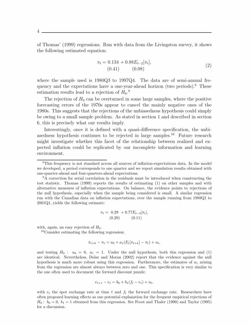
of Thomas’ (1999) regressions. Run with data from the Livingston survey, it showsthe following estimated equation:

πt = 0.134

(0.41)

+ 0.88Et−2[πt],

(0.08)(2)

where the sample used is 1980Q3 to 1997Q4. The data are of semi-annual fre-quency and the expectations have a one-year-ahead horizon (two periods).8 Theseestimation results lead to a rejection of H0.

9

The rejection of H0 can be overturned in some large samples, where the positiveforecasting errors of the 1970s appear to cancel the mainly negative ones of the1980s. This suggests that the rejections of the unbiasedness hypothesis could simplybe owing to a small sample problem. As stated in section 1 and described in section6, this is precisely what our results imply.

Interestingly, once it is defined with a quasi-difference specification, the unbi-asedness hypothesis continues to be rejected in large samples.10 Future researchmight investigate whether this facet of the relationship between realized and ex-pected inflation could be replicated by our incomplete information and learningenvironment.

8This frequency is not standard across all sources of inflation-expectations data. In the modelwe developed, a period corresponds to one quarter and we report simulation results obtained withone-quarter-ahead and four-quarters-ahead expectations.

9A correction for serial correlation in the residuals must be introduced when constructing thetest statistic. Thomas (1999) reports the results of estimating (1) on other samples and withalternative measures of inflation expectations. On balance, the evidence points to rejections ofthe null hypothesis, especially when the sample being considered is small. A similar regressionrun with the Canadian data on inflation expectations, over the sample running from 1988Q1 to2001Q1, yields the following estimate:

πt = 0.29(0.29)

+ 0.77Et−4[πt],(0.11)

with, again, an easy rejection of H0.10Consider estimating the following regression:

πt+k − πt = a0 + a1(Et[πt+k] − πt) + ut,

and testing H0 : a0 = 0, a1 = 1. Under the null hypothesis, both this regression and (1)are identical. Nevertheless, Dolar and Moran (2002) report that the evidence against the nullhypothesis is much more robust using this regression. Furthermore, the estimates of a1 arisingfrom the regression are almost always between zero and one. This specification is very similar tothe one often used to document the forward discount puzzle:

et+1 − et = b0 + b1(ft − et) + ut,

with et the spot exchange rate at time t and ft the forward exchange rate. Researchers haveoften proposed learning effects as one potential explanation for the frequent empirical rejections ofH0 : b0 = 0, b1 = 1 obtained from this regression. See Froot and Thaler (1990) and Taylor (1995)for a discussion.

5

3. The Model

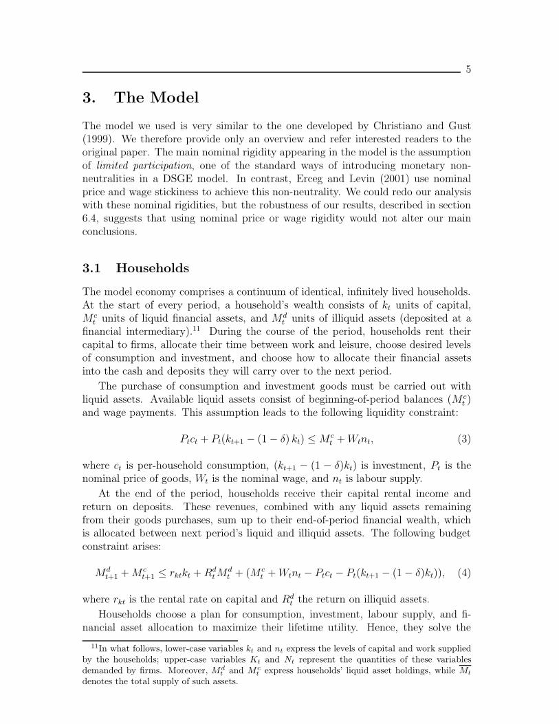
The model we used is very similar to the one developed by Christiano and Gust(1999). We therefore provide only an overview and refer interested readers to theoriginal paper. The main nominal rigidity appearing in the model is the assumptionof limited participation, one of the standard ways of introducing monetary non-neutralities in a DSGE model. In contrast, Erceg and Levin (2001) use nominalprice and wage stickiness to achieve this non-neutrality. We could redo our analysiswith these nominal rigidities, but the robustness of our results, described in section6.4, suggests that using nominal price or wage rigidity would not alter our mainconclusions.

3.1 Households

The model economy comprises a continuum of identical, infinitely lived households.At the start of every period, a household’s wealth consists of kt units of capital,M c

t units of liquid financial assets, and Mdt units of illiquid assets (deposited at a

financial intermediary).11 During the course of the period, households rent theircapital to firms, allocate their time between work and leisure, choose desired levelsof consumption and investment, and choose how to allocate their financial assetsinto the cash and deposits they will carry over to the next period.

The purchase of consumption and investment goods must be carried out withliquid assets. Available liquid assets consist of beginning-of-period balances (M c

t )and wage payments. This assumption leads to the following liquidity constraint:

Ptct + Pt(kt+1 − (1 − δ) kt) ≤ M ct +Wtnt, (3)

where ct is per-household consumption, (kt+1 − (1 − δ)kt) is investment, Pt is thenominal price of goods, Wt is the nominal wage, and nt is labour supply.

At the end of the period, households receive their capital rental income andreturn on deposits. These revenues, combined with any liquid assets remainingfrom their goods purchases, sum up to their end-of-period financial wealth, whichis allocated between next period’s liquid and illiquid assets. The following budgetconstraint arises:

Mdt+1 +M c

t+1 ≤ rktkt +RdtM

dt + (M c

t +Wtnt − Ptct − Pt(kt+1 − (1 − δ)kt)), (4)

where rkt is the rental rate on capital and Rdt the return on illiquid assets.

Households choose a plan for consumption, investment, labour supply, and fi-nancial asset allocation to maximize their lifetime utility. Hence, they solve the

11In what follows, lower-case variables kt and nt express the levels of capital and work suppliedby the households; upper-case variables Kt and Nt represent the quantities of these variablesdemanded by firms. Moreover, Md

t and M ct express households’ liquid asset holdings, while Mt

denotes the total supply of such assets.

6

following problem:

max[ct+k,nt+k,kt+k+1,M

ct+k+1,M

dt+k+1]|∞k=0

Et

∞∑k=0

ηt+kU(ct+k, nt+k + ACt+k) (5)

where U(., .) is the period utility function and η the time discount, and where themaximization is done with respect to (3),(4), and initial levels kt, M

ct , and Md

t .

The term nt+k + ACt+k represents the time costs of market activities, in termsof leisure foregone. The term ACt represents the costs households must incur toadjust their liquid asset portfolios. The functional form selected for these costs isas follows:12

ACt = τ(M ct+1/M

ct − µ)2, (6)

with µ the steady-state growth rate of the total supply of liquid assets.

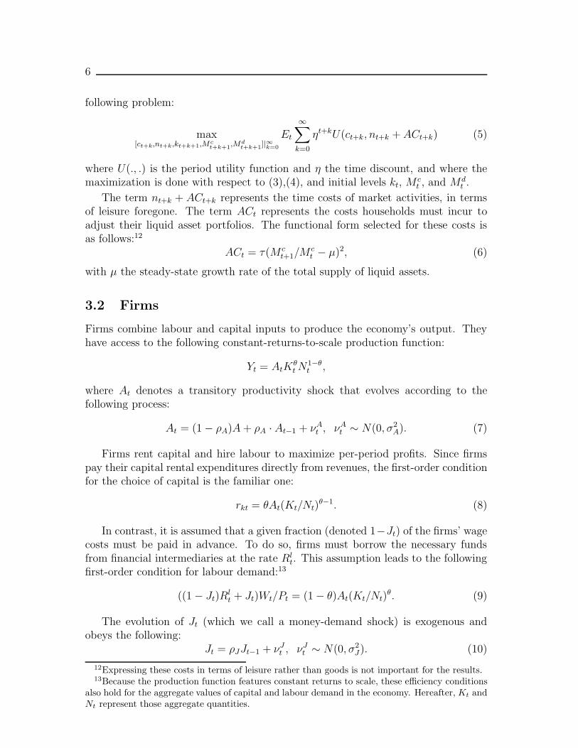
3.2 Firms

Firms combine labour and capital inputs to produce the economy’s output. Theyhave access to the following constant-returns-to-scale production function:

Yt = AtKθtN

1−θt ,

where At denotes a transitory productivity shock that evolves according to thefollowing process:

At = (1 − ρA)A+ ρA · At−1 + νAt , νAt ∼ N(0, σ2A). (7)

Firms rent capital and hire labour to maximize per-period profits. Since firmspay their capital rental expenditures directly from revenues, the first-order conditionfor the choice of capital is the familiar one:

rkt = θAt(Kt/Nt)θ−1. (8)

In contrast, it is assumed that a given fraction (denoted 1−Jt) of the firms’ wagecosts must be paid in advance. To do so, firms must borrow the necessary fundsfrom financial intermediaries at the rate Rl

t. This assumption leads to the followingfirst-order condition for labour demand:13

((1 − Jt)Rlt + Jt)Wt/Pt = (1 − θ)At(Kt/Nt)

θ. (9)

The evolution of Jt (which we call a money-demand shock) is exogenous andobeys the following:

Jt = ρJJt−1 + νJt , νJt ∼ N(0, σ2J). (10)

12Expressing these costs in terms of leisure rather than goods is not important for the results.13Because the production function features constant returns to scale, these efficiency conditions

also hold for the aggregate values of capital and labour demand in the economy. Hereafter, Kt andNt represent those aggregate quantities.

7

3.3 Financial intermediaries

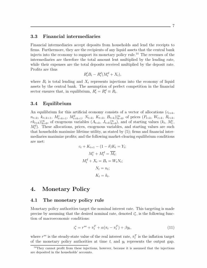
Financial intermediaries accept deposits from households and lend the receipts tofirms. Furthermore, they are the recipients of any liquid assets that the central bankinjects into the economy to support its monetary policy rule.14 The revenues of theintermediaries are therefore the total amount lent multiplied by the lending rate,while their expenses are the total deposits received multiplied by the deposit rate.Profits are thus

RltBt − Rd

t (Mdt +Xt),

where Bt is total lending and Xt represents injections into the economy of liquidassets by the central bank. The assumption of perfect competition in the financialsector ensures that, in equilibrium, Rl

t = Rdt ≡ Rt.

3.4 Equilibrium

An equilibrium for this artificial economy consists of a vector of allocations (ct+k,nt+k, kt+k+1, M

ct+k+1, M

dt+k+1, Nt+k, Kt+k, Bt+k)|∞k=0, of prices (Pt+k, Wt+k, Rt+k,

rkt+k)|∞k=0, of exogenous variables (At+k, Jt+k|∞k=0), and of starting values (kt, Mct ,

Mdt ). These allocations, prices, exogenous variables, and starting values are such

that households maximize lifetime utility, as stated by (5); firms and financial inter-mediaries maximize profits; and the following market-clearing equilibrium conditionsare met:

ct +Kt+1 − (1 − δ)Kt = Yt;

M ct +Md

t = Mt;

Mdt +Xt = Bt = WtNt;

Nt = nt;

Kt = kt.

4. Monetary Policy

4.1 The monetary policy rule

Monetary policy authorities target the nominal interest rate. This targeting is madeprecise by assuming that the desired nominal rate, denoted i∗t , is the following func-tion of macroeconomic conditions:

i∗t = rss + πTt + α(πt − πTt ) + βyt, (11)

where rss is the steady-state value of the real interest rate, πTt is the inflation targetof the monetary policy authorities at time t, and yt represents the output gap.

14They cannot profit from these injections, however, because it is assumed that the injectionsare deposited in the households’ accounts.

8

Note that rss + πTt represents the steady-state value of the nominal rate; (11) thussignifies that monetary authorities will increase rates relative to steady-state whenprice pressures threaten to push inflation over the current target, or when the outputgap is positive.

It is often conjectured that, instead of rapidly moving the nominal rate to reachthe targeted level, monetary policy authorities implement gradual changes in ratesthat only eventually converge to that level. Such a smoothing motive can be repre-sented mathematically by assuming that the actual rate implemented by the centralbank will be the following weighted sum of the targeted rate and the precedingperiod’s rate:

it = (1 − ρ)i∗t + ρit−1, (12)

where the coefficient ρ governs the extent of smoothing exercised by the monetarypolicy authorities.

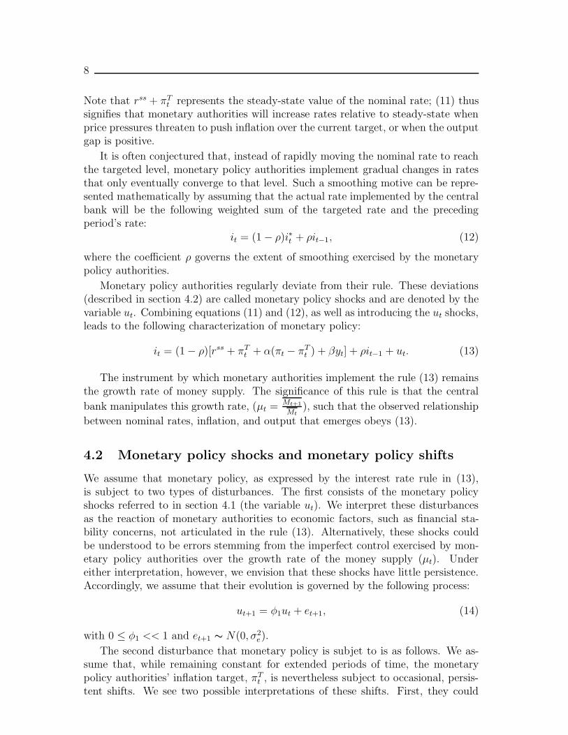
Monetary policy authorities regularly deviate from their rule. These deviations(described in section 4.2) are called monetary policy shocks and are denoted by thevariable ut. Combining equations (11) and (12), as well as introducing the ut shocks,leads to the following characterization of monetary policy:

it = (1 − ρ)[rss + πTt + α(πt − πTt ) + βyt] + ρit−1 + ut. (13)

The instrument by which monetary authorities implement the rule (13) remainsthe growth rate of money supply. The significance of this rule is that the central

bank manipulates this growth rate, (µt = Mt+1

Mt), such that the observed relationship

between nominal rates, inflation, and output that emerges obeys (13).

4.2 Monetary policy shocks and monetary policy shifts

We assume that monetary policy, as expressed by the interest rate rule in (13),is subject to two types of disturbances. The first consists of the monetary policyshocks referred to in section 4.1 (the variable ut). We interpret these disturbancesas the reaction of monetary authorities to economic factors, such as financial sta-bility concerns, not articulated in the rule (13). Alternatively, these shocks couldbe understood to be errors stemming from the imperfect control exercised by mon-etary policy authorities over the growth rate of the money supply (µt). Undereither interpretation, however, we envision that these shocks have little persistence.Accordingly, we assume that their evolution is governed by the following process:

ut+1 = φ1ut + et+1, (14)

with 0 ≤ φ1 << 1 and et+1 ∼ N(0, σ2e).

The second disturbance that monetary policy is subjet to is as follows. We as-sume that, while remaining constant for extended periods of time, the monetarypolicy authorities’ inflation target, πTt , is nevertheless subject to occasional, persis-tent shifts. We see two possible interpretations of these shifts. First, they could

9

correspond with changes in economic thinking that lead monetary policy author-ities to modify their views about the proper rate of inflation to pursue. DeLong(1997), for example, argues that the Great Inflation of the 1970s, and its eventualtermination by the Federal Reserve at the beginning of the 1980s, was a result ofshifting views about the shape of the Philips curve and, more generally, about thenature of the constraints under which monetary policy is conducted. Alternatively,a change in the inflation target could reflect the appointment of a new central bankhead, whose preferences for inflation outcomes differ from their predecessor’s. Undereither interpretation, we envision that these shifts will have a significant duration,in the order of, say, five to ten years.

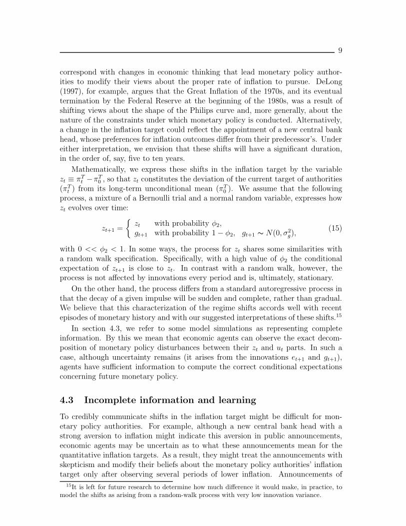
Mathematically, we express these shifts in the inflation target by the variablezt ≡ πTt −πT0 , so that zt constitutes the deviation of the current target of authorities(πTt ) from its long-term unconditional mean (πT0 ). We assume that the followingprocess, a mixture of a Bernoulli trial and a normal random variable, expresses howzt evolves over time:

zt+1 =

{zt with probability φ2,gt+1 with probability 1 − φ2, gt+1 ∼ N(0, σ2

g),(15)

with 0 << φ2 < 1. In some ways, the process for zt shares some similarities witha random walk specification. Specifically, with a high value of φ2 the conditionalexpectation of zt+1 is close to zt. In contrast with a random walk, however, theprocess is not affected by innovations every period and is, ultimately, stationary.

On the other hand, the process differs from a standard autoregressive process inthat the decay of a given impulse will be sudden and complete, rather than gradual.We believe that this characterization of the regime shifts accords well with recentepisodes of monetary history and with our suggested interpretations of these shifts.15

In section 4.3, we refer to some model simulations as representing completeinformation. By this we mean that economic agents can observe the exact decom-position of monetary policy disturbances between their zt and ut parts. In such acase, although uncertainty remains (it arises from the innovations et+1 and gt+1),agents have sufficient information to compute the correct conditional expectationsconcerning future monetary policy.

4.3 Incomplete information and learning

To credibly communicate shifts in the inflation target might be difficult for mon-etary policy authorities. For example, although a new central bank head with astrong aversion to inflation might indicate this aversion in public announcements,economic agents may be uncertain as to what these announcements mean for thequantitative inflation targets. As a result, they might treat the announcements withskepticism and modify their beliefs about the monetary policy authorities’ inflationtarget only after observing several periods of lower inflation. Announcements of

15It is left for future research to determine how much difference it would make, in practice, tomodel the shifts as arising from a random-walk process with very low innovation variance.

10

explicit, quantitative changes in the inflation target might suffer, at least initially,from similar credibility problems.16 Alternatively, central banks sometimes do notmake explicit announcements about their inflation target, but let economic agentsdecipher as best they can announcements of a more general nature.

To capture the spirit of this information problem, we assume that the zt shiftsare unobservable to economic agents. They observe only a mixture of the zt shiftsand the ut shocks. Agents thus face a signal-extraction problem that is solved usingthe Kalman filter.

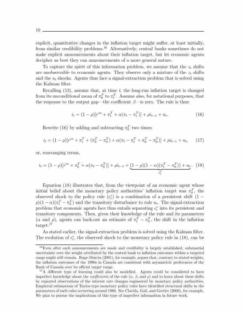
Recalling (13), assume that, at time t, the long-run inflation target is changedfrom its unconditional mean of πT0 to πTt . Assume also, for notational purposes, thatthe response to the output gap—the coefficient β—is zero. The rule is thus:

it = (1 − ρ)[rss + πTt + α(πt − πTt )] + ρit−1 + ut. (16)

Rewrite (16) by adding and subtracting πT0 two times:

it = (1 − ρ)[rss + πTt + (πT0 − πT0 ) + α(πt − πTt + πT0 − πT0 )] + ρit−1 + ut, (17)

or, rearranging terms,

it = (1 − ρ)[rss + πT0 + α(πt − πT0 )] + ρit−1 + (1 − ρ)(1 − α)(πTt − πT0 )) + ut︸ ︷︷ ︸ε∗t

. (18)

Equation (18) illustrates that, from the viewpoint of an economic agent whoseinitial belief about the monetary policy authorities’ inflation target was πT0 , theobserved shock to the policy rule (ε∗t ) is a combination of a persistent shift (1 −ρ)(1−α)(πTt − πT0 ) and the transitory disturbance to rule ut. The signal-extractionproblem that economic agents face thus entails separating ε∗t into its persistent andtransitory components. Then, given their knowledge of the rule and its parameters(α and ρ), agents can back-out an estimate of πTt − πT0 , the shift in the inflationtarget.17

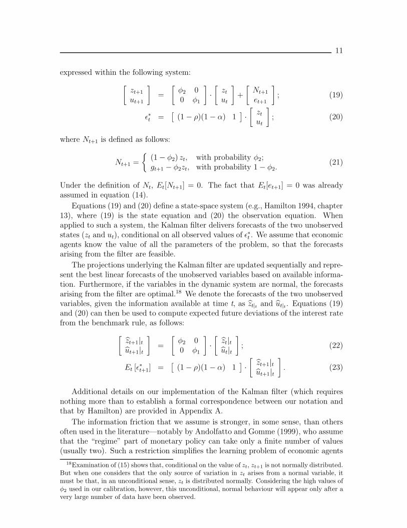
As stated earlier, the signal-extraction problem is solved using the Kalman filter.The evolution of ε∗t , the observed shock to the monetary policy rule in (18), can be

16Even after such announcements are made and credibility is largely established, substantialuncertainty over the weight attributed by the central bank to inflation outcomes within a targetedrange might still remain. Ruge-Murcia (2001), for example, argues that, contrary to stated weights,the inflation outcomes of the 1990s in Canada are consistent with asymmetric preferences of theBank of Canada over its official target range.

17A different type of learning could also be modelled. Agents could be considered to haveimperfect knowledge about the coefficients of the rule (α, β, and ρ) and to learn about these shiftsby repeated observations of the interest rate changes engineered by monetary policy authorities.Empirical estimations of Taylor-type monetary policy rules have identified structural shifts in theparameters of such rules occurring around 1980. See Clarida, Galı, and Gertler (2000), for example.We plan to pursue the implications of this type of imperfect information in future work.

11

expressed within the following system:[zt+1

ut+1

]=

[φ2 00 φ1

]·[ztut

]+

[Nt+1

et+1

]; (19)

ε∗t =[

(1 − ρ)(1 − α) 1] · [ zt

ut

]; (20)

where Nt+1 is defined as follows:

Nt+1 =

{(1 − φ2) zt, with probability φ2;gt+1 − φ2zt, with probability 1 − φ2.

(21)

Under the definition of Nt, Et[Nt+1] = 0. The fact that Et[et+1] = 0 was alreadyassumed in equation (14).

Equations (19) and (20) define a state-space system (e.g., Hamilton 1994, chapter13), where (19) is the state equation and (20) the observation equation. Whenapplied to such a system, the Kalman filter delivers forecasts of the two unobservedstates (zt and ut), conditional on all observed values of ε∗t . We assume that economicagents know the value of all the parameters of the problem, so that the forecastsarising from the filter are feasible.

The projections underlying the Kalman filter are updated sequentially and repre-sent the best linear forecasts of the unobserved variables based on available informa-tion. Furthermore, if the variables in the dynamic system are normal, the forecastsarising from the filter are optimal.18 We denote the forecasts of the two unobservedvariables, given the information available at time t, as zt|t and ut|t . Equations (19)and (20) can then be used to compute expected future deviations of the interest ratefrom the benchmark rule, as follows:[

zt+1|tut+1|t

]=

[φ2 00 φ1

]·[zt|tut|t

]; (22)

Et [ε∗t+1] =

[(1 − ρ)(1 − α) 1

] · [ zt+1|tut+1|t

]. (23)

Additional details on our implementation of the Kalman filter (which requiresnothing more than to establish a formal correspondence between our notation andthat by Hamilton) are provided in Appendix A.

The information friction that we assume is stronger, in some sense, than othersoften used in the literature—notably by Andolfatto and Gomme (1999), who assumethat the “regime” part of monetary policy can take only a finite number of values(usually two). Such a restriction simplifies the learning problem of economic agents

18Examination of (15) shows that, conditional on the value of zt, zt+1 is not normally distributed.But when one considers that the only source of variation in zt arises from a normal variable, itmust be that, in an unconditional sense, zt is distributed normally. Considering the high values ofφ2 used in our calibration, however, this unconditional, normal behaviour will appear only after avery large number of data have been observed.

12

and usually produces quick transition of the beliefs following regime shifts. We con-sider, however, that these “two-point” learning problems understate the severity ofthe information friction over monetary policy faced by real-world economic agents.19

5. Calibration and Solution of the Model

Three distinct areas of the model require calibration: the model itself (preferences,technology, etc.), the parameters of the interest rate rule (13), and the parametersgoverning the evolution of the shocks and shifts in the rule. The model periodcorresponds to one quarter.

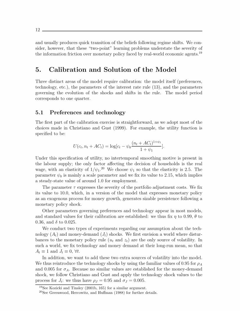
5.1 Preferences and technology

The first part of the calibration exercise is straightforward, as we adopt most of thechoices made in Christiano and Gust (1999). For example, the utility function isspecified to be:

U(ct, nt + ACt) = log[ct − ψ0(nt + ACt)

1+ψ1

1 + ψ1].

Under this specification of utility, no intertemporal smoothing motive is present inthe labour supply; the only factor affecting the decision of households is the realwage, with an elasticity of 1/ψ1.

20 We choose ψ1 so that the elasticity is 2.5. Theparameter ψ0 is mainly a scale parameter and we fix its value to 2.15, which impliesa steady-state value of around 1.0 for employment.

The parameter τ expresses the severity of the portfolio adjustment costs. We fixits value to 10.0, which, in a version of the model that expresses monetary policyas an exogenous process for money growth, generates sizable persistence following amonetary policy shock.

Other parameters governing preferences and technology appear in most models,and standard values for their calibration are established: we thus fix η to 0.99, θ to0.36, and δ to 0.025.

We conduct two types of experiments regarding our assumption about the tech-nology (At) and money-demand (Jt) shocks. We first envision a world where distur-bances to the monetary policy rule (ut and zt) are the only source of volatility. Insuch a world, we fix technology and money demand at their long-run mean, so thatAt ≡ 1 and Jt ≡ 0, ∀t.

In addition, we want to add these two extra sources of volatility into the model.We thus reintroduce the technology shocks by using the familiar values of 0.95 for ρAand 0.005 for σA. Because no similar values are established for the money-demandshock, we follow Christiano and Gust and apply the technology shock values to theprocess for Jt: we thus have ρJ = 0.95 and σJ = 0.005.

19See Kozicki and Tinsley (2001b, 165) for a similar argument.20See Greenwood, Hercowitz, and Huffman (1988) for further details.

13

The model is solved using the first-order approximation method and algorithmsgiven in King and Watson (1998). Details of the solution method are available fromthe authors upon request.

5.2 Parameters of the interest-rate-targeting rule

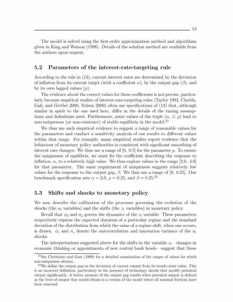
According to the rule in (13), current interest rates are determined by the deviationof inflation from its current target (with a coefficient α), by the output gap (β), andby its own lagged values (ρ).

The evidence about the correct values for these coefficients is not precise, particu-larly because empirical studies of interest-rate-targeting rules (Taylor 1993, Clarida,Galı, and Gertler 2000, Nelson 2000) often use specifications of (13) that, althoughsimilar in spirit to the one used here, differ in the details of the timing assump-tions and definitions used. Furthermore, some values of the triple (α, β, ρ) lead tonon-uniqueness (or non-existence) of stable equilibria in the model.21

We thus use such empirical evidence to suggest a range of reasonable values forthe parameters and conduct a sensitivity analysis of our results to different valueswithin that range. For example, many empirical studies report evidence that thebehaviour of monetary policy authorities is consistent with significant smoothing ofinterest rate changes. We thus use a range of [0, 0.5] for the parameter ρ. To ensurethe uniqueness of equilibria, we must fix the coefficient describing the response toinflation, α, to a relatively high value. We thus explore values in the range [2.0, 4.0]for that parameter. The same requirement of uniqueness suggests relatively lowvalues for the response to the output gap, β. We thus use a range of [0, 0.25]. Ourbenchmark specification sets α = 2.0, ρ = 0.25, and β = 0.25.22

5.3 Shifts and shocks to monetary policy

We now describe the calibration of the processes governing the evolution of theshocks (the ut variables) and the shifts (the zt variables) in monetary policy.

Recall that φ2 and σg govern the dynamics of the zt variable. These parametersrespectively express the expected duration of a particular regime and the standarddeviation of the distribution from which the value of a regime shift, when one occurs,is drawn. φ1 and σe denote the autocorrelation and innovation variance of the utshocks.

The interpretations suggested above for the shifts in the variable zt—changes ineconomic thinking or appointments of new central bank heads—suggest that these

21See Christiano and Gust (1999) for a detailed examination of the ranges of values for whichnon-uniqueness obtains.

22We define the output gap as the deviation of current output from its steady-state value. Thisis an incorrect definition, particularly in the presence of technology shocks that modify potentialoutput significantly. A better measure of the output gap results when potential output is definedas the level of output that would obtain in a version of the model where all nominal frictions havebeen removed.

14

shifts occur only infrequently, perhaps once every five or ten years. Transposed tothe quarterly frequency we use, this corresponds to one shift, on average, every 20to 40 periods. Such an average duration between shifts corresponds to values of φ2

between 0.95 and 0.975. We use the slightly wider range of [0.95, 0.99] for φ2, with0.975 as the benchmark value.

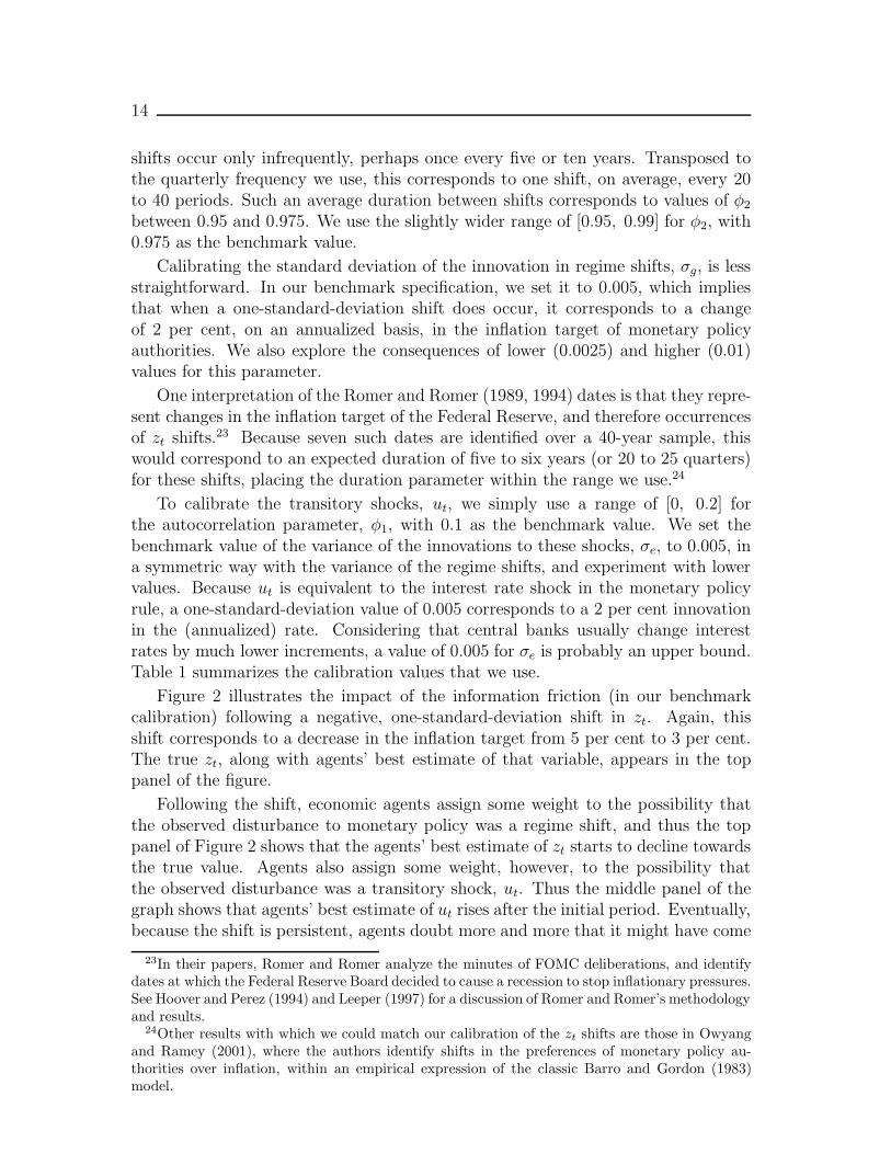
Calibrating the standard deviation of the innovation in regime shifts, σg, is lessstraightforward. In our benchmark specification, we set it to 0.005, which impliesthat when a one-standard-deviation shift does occur, it corresponds to a changeof 2 per cent, on an annualized basis, in the inflation target of monetary policyauthorities. We also explore the consequences of lower (0.0025) and higher (0.01)values for this parameter.

One interpretation of the Romer and Romer (1989, 1994) dates is that they repre-sent changes in the inflation target of the Federal Reserve, and therefore occurrencesof zt shifts.23 Because seven such dates are identified over a 40-year sample, thiswould correspond to an expected duration of five to six years (or 20 to 25 quarters)for these shifts, placing the duration parameter within the range we use.24

To calibrate the transitory shocks, ut, we simply use a range of [0, 0.2] forthe autocorrelation parameter, φ1, with 0.1 as the benchmark value. We set thebenchmark value of the variance of the innovations to these shocks, σe, to 0.005, ina symmetric way with the variance of the regime shifts, and experiment with lowervalues. Because ut is equivalent to the interest rate shock in the monetary policyrule, a one-standard-deviation value of 0.005 corresponds to a 2 per cent innovationin the (annualized) rate. Considering that central banks usually change interestrates by much lower increments, a value of 0.005 for σe is probably an upper bound.Table 1 summarizes the calibration values that we use.

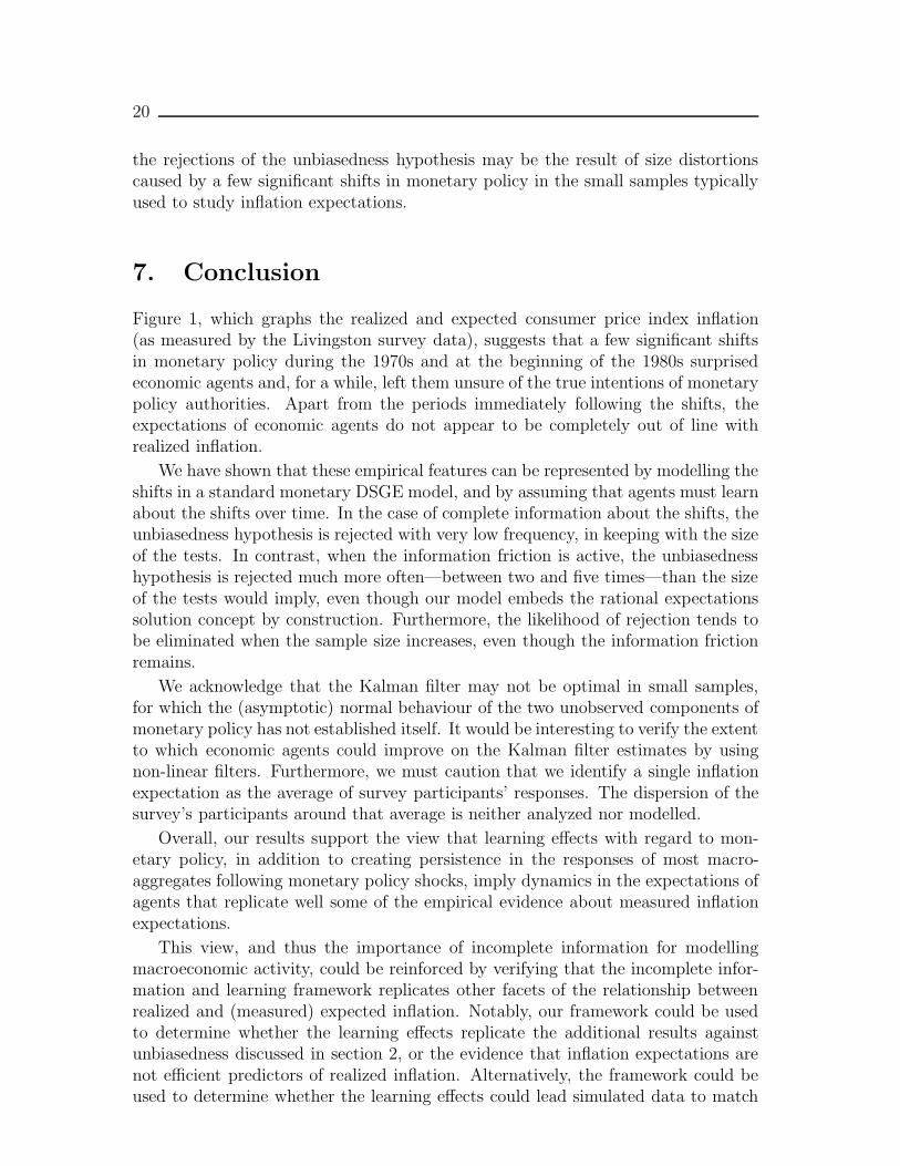
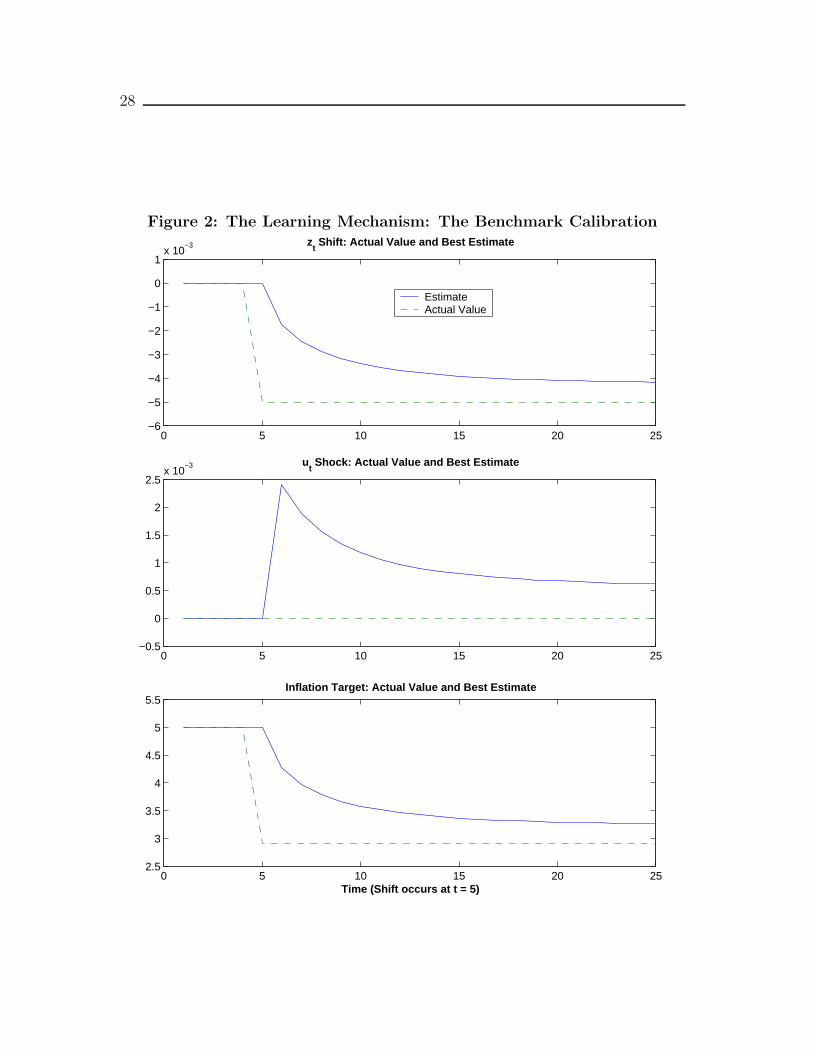
Figure 2 illustrates the impact of the information friction (in our benchmarkcalibration) following a negative, one-standard-deviation shift in zt. Again, thisshift corresponds to a decrease in the inflation target from 5 per cent to 3 per cent.The true zt, along with agents’ best estimate of that variable, appears in the toppanel of the figure.

Following the shift, economic agents assign some weight to the possibility thatthe observed disturbance to monetary policy was a regime shift, and thus the toppanel of Figure 2 shows that the agents’ best estimate of zt starts to decline towardsthe true value. Agents also assign some weight, however, to the possibility thatthe observed disturbance was a transitory shock, ut. Thus the middle panel of thegraph shows that agents’ best estimate of ut rises after the initial period. Eventually,because the shift is persistent, agents doubt more and more that it might have come

23In their papers, Romer and Romer analyze the minutes of FOMC deliberations, and identifydates at which the Federal Reserve Board decided to cause a recession to stop inflationary pressures.See Hoover and Perez (1994) and Leeper (1997) for a discussion of Romer and Romer’s methodologyand results.

24Other results with which we could match our calibration of the zt shifts are those in Owyangand Ramey (2001), where the authors identify shifts in the preferences of monetary policy au-thorities over inflation, within an empirical expression of the classic Barro and Gordon (1983)model.

15

from the largely transitory ut, and they become convinced that it must have comefrom a zt shift. Accordingly, the agents’ best estimate of zt and ut, respectively,converges towards the true value and to zero.

The bottom panel of Figure 2 shows the progress of the agents’ estimate of themonetary policy authorities’ annualized inflation target (implied by their estimatesof zt: recall the definition of ε∗t in equation (18)). The panel shows that beliefssmoothly converge towards the true value of 3 per cent.

6. Monte Carlo Simulation of the Model

6.1 Impulse responses following a regime shift

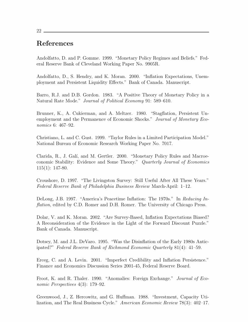
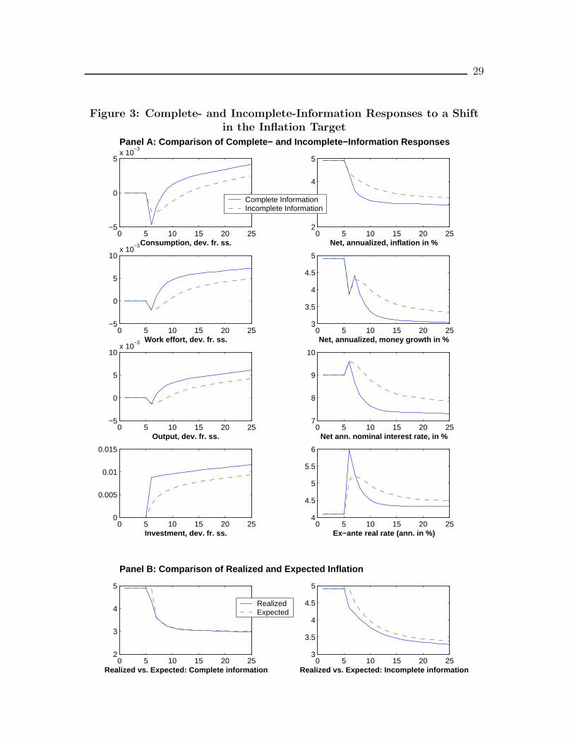
To develop intuition about the Monte Carlo results that follow, Figure 3 shows theimpulse responses of the artificial economy following a shift in the monetary policyauthorities’ inflation target. The shift is identical to the one illustrated in Figure 2:the inflation target is lowered, at time t = 5, from 5 per cent on an annualized basisto 3 per cent.

In Panel A of Figure 3, the solid lines represent the case where agents havecomplete information about the shift. In contrast, the dashed lines represent thecase where information friction is active and the learning mechanism governs theformation of expectations.

The solid lines indicate that, following the implementation of the monetary policyshift, a very short downturn affects the economy: consumption, output, and employ-ment shrink for only one or two periods. Very rapidly, the positive, long-term effectsof the decrease in inflation begin to take hold and all real variables increase, passingtheir initial levels and converging towards a higher steady-state. The dashed linesindicate that, in the incomplete-information case, this process takes several periodsto firmly establish itself, during which all real aggregates are lower than they werein the full-information case. This occurs because economic agents assign a positiveprobability to the interest rate shock being a transitory hike in interest rates, withstraightforward negative effects on the real economy.

Panel B of Figure 3 illustrates the situation from a slightly different angle. Thesolid lines depict realized inflation, and the dashed lines expected inflation. The leftgraph in Panel B shows the complete-information case: apart from the initial surprisein the first period of the shock, economic agents have the correct inflation expecta-tions. The right graph in Panel B depicts the incomplete-information case: inflationexpectations lag actual inflation for several periods before converging. This featurereplicates, in a qualitative fashion, the behaviour of inflation expectations duringthe 1980s, as shown in Figure 1. In that figure, during a period of generally decreas-ing inflation, expectations—as measured by the Livingston survey—overpredictedactual numbers for several quarters.

The gap between realized and expected inflation in the right graph of Panel B,Figure 3, is a direct result of the learning behaviour described in section 4. Initially,

16

agents assign some weight to the possibility that the observed monetary disturbancewas a transitory disturbance to the rule. They therefore do not expect it to lastand they think that inflation might return to the initial, higher level of 5 per cent.Over time, agents become convinced that a shift has indeed occurred and theirexpectations converge to values that are closer to the actual ones.

In the simulations performed using the model, transitory shocks occur simulta-neously with the shifts in the inflation target; therefore, a picture of the artificialeconomy’s responses will not be very informative. The main picture given by thegraphs in Figure 3, however, remains: when a shift occurs, agents are likely to un-derestimate them for some time, and inflation expectations are likely to erroneouslypredict actual inflation for some time. It remains to be seen whether this effect isstrong enough to generate empirical rejections of the unbiasedness hypothesis.

6.2 The experiment

We treat our model as if it was the true data generating process (DGP) of economicvariables, and assess what an empirical researcher, given outcomes from this DGP,would conclude about the unbiasedness of inflation expectations. To this end, MonteCarlo simulations of the model economy are performed 1000 times.

In each of these simulations, a random realization of 80 periods is generated forboth unobserved disturbances to the interest rate rule (the ut and zt variables).25

Economic agents’ estimates of these shocks are computed and the model is solvedaccording to this information. Two alternative measures of inflation, one-quarter-ahead inflation (πt ≡ Pt+1/Pt) and four-quarters-ahead inflation (πt ≡ Pt+4/Pt),are stored, along with the corresponding expectations of these quantities (πet ≡Et[Pt+1/Pt] and πet ≡ Et[Pt+4/Pt]).

Next, for each of these simulations, we perform the unbiasedness test describedin section 2. Recall that this involves estimating the regression

πt = a0 + a1πet + εt, (24)

and testing the null hypothesis H0 : a0 = 0; a1 = 1. For each simulation, we recordthe estimates a0 and a1, as well as the appropriate test statistic about H0.

26

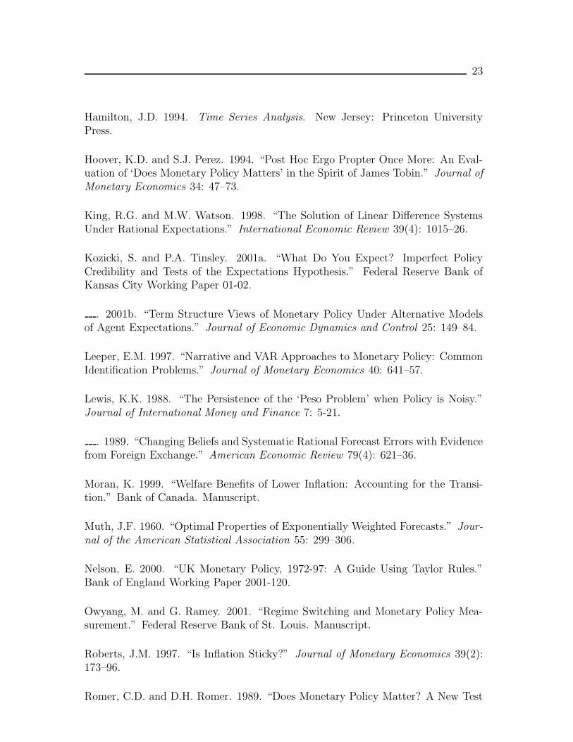
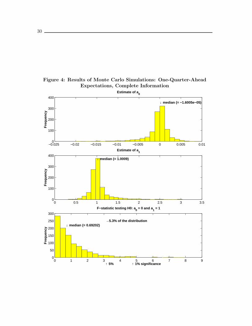
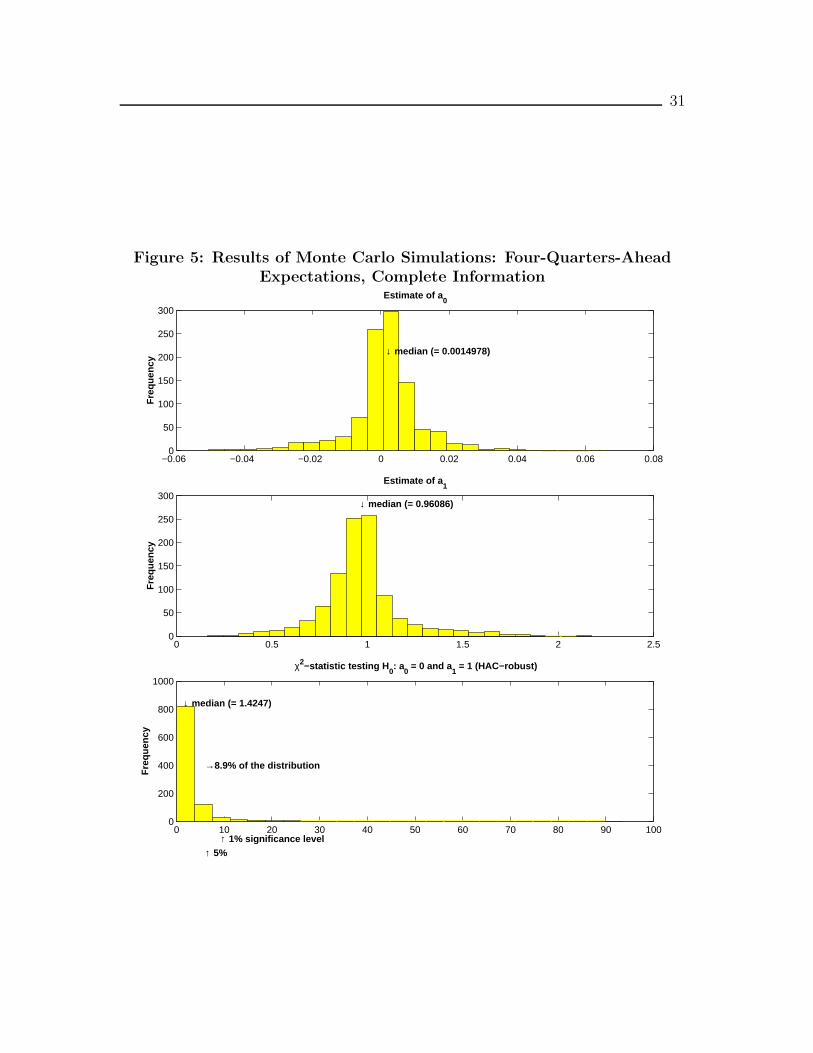
Figures 4 to 7 show the results of these simulations using the benchmark calibra-tion. In each of those figures, the top panel is a histogram that depicts the estimatesof a0 across the 1000 replications. It also depicts the median of the estimates. Themiddle panel depicts the estimates of a1, again identifying the median. The bottom

25The empirical rejections of the unbiasedness hypothesis described in section 2 are typicallyobtained with data samples of limited length.

26Under the null hypothesis and for one-quarter-ahead expectations, the expectation errors (theresiduals in (24)) should not be serially correlated and we therefore use a simple F -statistic to testH0. In the case of four-quarters-ahead expectations, the expectation errors would be correlated upto three lags even under H0, because of the overlap between the horizon of the expectations andthe frequency of the data. We thus use the Newey-West procedure to correct for serial correlationwhen computing the standard errors of the estimates. The test statistic is distributed as a χ2.

17

panel illustrates the results of the 1000 tests of H0, showing a histogram of the teststatistic along with its median and the 5 per cent and 1 per cent critical valuesassociated with the test. We also indicate the fraction of the simulations for whichthe test statistic rejects H0 at a significance level better than 5 per cent. Whenthe null hypothesis is true and the test is correctly specified, this fraction shouldbe close to 5 per cent, the size of the test. On the other hand, one can interpretresults where this fraction is significantly higher than 5 per cent to suggest that thelearning effects reduce the capability of the test to properly identify unbiasedness.

6.3 Results for the benchmark case

Figures 4 and 5 illustrate the cases of one-quarter-ahead and four-quarters-aheadexpectations, respectively, when information is complete. Figures 6 and 7 illus-trate the cases of one-quarter-ahead and four-quarters-ahead expectations for theincomplete-information case, in which the information friction that we emphasizedis activated.

The top panel of Figure 4 is a histogram that depicts the estimates of a0 acrossthe 1000 replications. It shows that the median estimate of a0 is very close to zero.Similarly, the middle panel, which depicts the estimates of a1, shows a median veryclose to the hypothesized value of 1. The bottom panel confirms that these deviationsfrom the respective values of 0 for α0 and 1 for α1 were not often significant: the teststatistic for the hypothesis has a median around 0.70, when the 5 per cent rejectionregion starts above 3. In fact, only 5.3 per cent of the simulations lead the teststatistic to reject the null at better than the 5 per cent significance level. It appearsthat, in the case of one-quarter-ahead expectations with complete information, theunbiasedness test performs just as it should.

Figure 5 depicts the case when inflation expectations are measured as four-quarters-ahead expectations, with the information still complete. While the esti-mates of a0 remain close to zero, the middle panel of the figure shows that themedian estimate of a1 is now around 0.96. The correction for serial correlation,however, makes rejections harder to achieve, so that the test statistic rejects thenull hypothesis in only about 9 per cent of the cases, not drastically away from the5 per cent size of the test.

Overall, the complete-information results in Figures 4 and 5 suggest that, insuch an economy, the simple tests of unbiasedness that are often performed in theempirical literature behave much as they should.

Let us now examine the cases for which the information friction is activated.Figure 6 shows that, for the one-quarter-ahead expectations, while the estimate ofthe constant parameter is again not drastically different from zero, the distributionof the slope estimates is significantly skewed away from the hypothesized value of 1,yielding a median value of 0.82. The bottom panel of Figure 6 illustrates that thisskewness is reflected in the number of times H0 is rejected: more than 20 per centof the cases feature a rejection of the null hypothesis, even though, by construction,our solution embodies the “rational expectations” hypothesis.

18

Figure 7 shows that, for the case of four-quarters-ahead expectations with incom-plete information, results are similar to those in Figure 6: the slope estimates aredistributed significantly away from the hypothesized value of 1 and imply rejectionsof H0 that are about five times more frequent than the normal rate of 5 per cent.

These benchmark results suggest that the joint hypothesis of the model, thelearning mechanism, and the calibration of the problem introduce significant sizedistortions in unbiasedness tests of inflation expectations. These distortions arisebecause the relatively small samples with which these tests are performed are dom-inated by a few significant shifts in monetary policy that surprise agents and leadthem, at least initially, to be confused about the true intentions of monetary policyauthorities. Section 6.4 analyzes the extent to which the qualitative nature of theresults expressed in Figures 4 to 7 are sensitive to the calibration of the model.

6.4 Sensitivity analysis

To analyze the sensitivity of the results to modifications in the calibration, we redothe above analysis for several alternative specifications. Table 2 reports the results.Column one indicates the kind of departure from the benchmark calibration thatis under study. Columns two and three indicate the frequency with which the un-biasedness hypothesis is rejected when one-quarter-ahead expectations are used, inthe complete-information and incomplete-information cases, respectively. Columnsfour and five report the corresponding results when the four-quarters-ahead expec-tations are utilized. To facilitate the comparison, the results from the benchmarkcases are repeated at the beginning of the table.

Table 2 gives the general impression that the complete-information cases generaterejections of H0 as often, roughly, as the size of the tests implies. Particularly incolumn one, the fraction of rejections seldom departs significantly from the level(5 per cent) suggested by the size of the test. Although the numbers in columnthree do depart more significantly from 5 per cent, the departures are never excessive.In contrast, the incomplete-information cases feature rejections of H0 that are farmore frequent. Although the precise numbers change from one case to the next, weobserve rejections of H0 two to five times more often when the information frictionis activated. Interestingly, the fraction of rejections does not seem to depend uponwhether one-quarter-ahead or four-quarters-ahead expectations are used.

For specific cases, in the first three departures from the benchmark case, elimi-nating the response of monetary policy authorities to the output gap or modifyingthe extent to which interest rate changes are smoothed-in does not change the resultsmarkedly. However, increasing the aggressiveness of the monetary policy authori-ties’ response to deviations of inflation from the target (an increase of α from 2.0 toeither 3.0 or 4.0) does modify the results substantially. The unbiasedness hypothe-sis is then rejected around 35 per cent of the time when the information friction isactive, while the corresponding numbers for the complete-information case increaseonly slightly. The frequency of rejections increases because a high value for the co-efficient α acts like a multiplier on the monetary policy shift. This is best illustrated

19

by recalling the definition of ε∗t in (18): a high value of α implies, for a given shift(πt − πT0 ), a stronger increase in interest rates.27

We also experiment with modifications to the processes governing the evolutionof the two components to monetary policy. We modify the expected duration of agiven shift in zt, first from 0.975 to 0.99, then back to 0.95. Increasing the durationopens the gap between the complete- and incomplete-information cases somewhat,compared with the benchmark case. Decreasing the duration closes that gap. Modi-fications to the persistence of the transitory shocks, the next departures from bench-mark that we consider, do not modify the results markedly. Next, we experimentwith changes in the variances of the shocks and shifts. These experiments showthat increasing the variance in the shifts zt, relative to the variance of the shocksut, increases the gap between the complete- and incomplete-information cases. Con-sidering our previous assessment that the benchmark value for the variance in theshocks ut (the parameter σe) is an upper bound, this result points to significant andcontinued differences between the complete- and incomplete-information cases.

The last series of modifications to the benchmark calibration, in Panel C of Ta-ble 2, bring interesting observations. First, increasing the number of repetitions forthe benchmark case (to 2500 from 1000) brings only small changes to the results.This experiment shows that 1000 repetitions is enough to get a good sense of thepopulation distribution of the test statistics. Second, Panel C shows that modifyingthe level of the costs of adjustments in the portfolio of economic agents or includ-ing money-demand shocks as specified in (9) and (10) does not change the resultssignificantly.

On the other hand, adding technology shocks, as specified in (7), attenuatesthe difference between the complete- and incomplete-information cases. Such a re-sult actually validates our approach; because the technology shocks are perfectlyobserved by both economic agents and monetary policy authorities, one does notexpect that the introduction of those shocks would imply a distorted relationshipbetween realized and expected inflation. The rejections of the unbiasedness hypoth-esis that we identify thus truly arise from the limited information about monetarypolicy shocks.28

The last experiment shows that using 1000 repetitions of much longer samples(with 500 periods in each sample) drastically reduces the rejections, particularlyfor the incomplete-information case. This last experiment strongly suggests that

27While it may seem that stronger shifts would make learning easier, the high duration of a givenshift implies that economic agents will not, at first, identify even sharp spikes in interest rates asarising from shifts in the inflation target. This intuition is also at play when the departure frombenchmark analyzed is an increase in the standard deviation of the shifts themselves.

28Of course, the belief that macroeconomic volatility in the last 40 years was solely the result oftechnology shocks would imply, in the environment we describe, that the empirical rejections of theunbiasedness hypothesis could not have come from learning about monetary policy. We believe,however, that ample evidence exists of very significant monetary policy shocks having affected themacroeconomic outcomes of all major economies in the last 40 years. In an environment withlearning about the parameters of the monetary policy rule, technology shocks could potentiallyaffect learning about monetary policy to a greater degree.

20

the rejections of the unbiasedness hypothesis may be the result of size distortionscaused by a few significant shifts in monetary policy in the small samples typicallyused to study inflation expectations.

7. Conclusion

Figure 1, which graphs the realized and expected consumer price index inflation(as measured by the Livingston survey data), suggests that a few significant shiftsin monetary policy during the 1970s and at the beginning of the 1980s surprisedeconomic agents and, for a while, left them unsure of the true intentions of monetarypolicy authorities. Apart from the periods immediately following the shifts, theexpectations of economic agents do not appear to be completely out of line withrealized inflation.

We have shown that these empirical features can be represented by modelling theshifts in a standard monetary DSGE model, and by assuming that agents must learnabout the shifts over time. In the case of complete information about the shifts, theunbiasedness hypothesis is rejected with very low frequency, in keeping with the sizeof the tests. In contrast, when the information friction is active, the unbiasednesshypothesis is rejected much more often—between two and five times—than the sizeof the tests would imply, even though our model embeds the rational expectationssolution concept by construction. Furthermore, the likelihood of rejection tends tobe eliminated when the sample size increases, even though the information frictionremains.

We acknowledge that the Kalman filter may not be optimal in small samples,for which the (asymptotic) normal behaviour of the two unobserved components ofmonetary policy has not established itself. It would be interesting to verify the extentto which economic agents could improve on the Kalman filter estimates by usingnon-linear filters. Furthermore, we must caution that we identify a single inflationexpectation as the average of survey participants’ responses. The dispersion of thesurvey’s participants around that average is neither analyzed nor modelled.

Overall, our results support the view that learning effects with regard to mon-etary policy, in addition to creating persistence in the responses of most macro-aggregates following monetary policy shocks, imply dynamics in the expectations ofagents that replicate well some of the empirical evidence about measured inflationexpectations.

This view, and thus the importance of incomplete information for modellingmacroeconomic activity, could be reinforced by verifying that the incomplete infor-mation and learning framework replicates other facets of the relationship betweenrealized and (measured) expected inflation. Notably, our framework could be usedto determine whether the learning effects replicate the additional results againstunbiasedness discussed in section 2, or the evidence that inflation expectations arenot efficient predictors of realized inflation. Alternatively, the framework could beused to determine whether the learning effects could lead simulated data to match

21

the dynamic correlation patterns linking realized and expected inflation.

The evidence of shifts in the parameters of the interest rate rule (see Clarida,Galı, and Gertler 2000) opens interesting avenues for future research. Straightfor-ward modifications to our framework could be used to determine whether such shifts,and least-square learning about the shifts on the part of economic agents, are re-sponsible for the evidence against unbiasedness and efficiency in measured inflationexpectations.

22

References

Andolfatto, D. and P. Gomme. 1999. “Monetary Policy Regimes and Beliefs.” Fed-eral Reserve Bank of Cleveland Working Paper No. 9905R.

Andolfatto, D., S. Hendry, and K. Moran. 2000. “Inflation Expectations, Unem-ployment and Persistent Liquidity Effects.” Bank of Canada. Manuscript.

Barro, R.J. and D.B. Gordon. 1983. “A Positive Theory of Monetary Policy in aNatural Rate Mode.” Journal of Political Economy 91: 589–610.

Brunner, K., A. Cukierman, and A. Meltzer. 1980. “Stagflation, Persistent Un-employment and the Permanence of Economic Shocks.” Journal of Monetary Eco-nomics 6: 467–92.

Christiano, L. and C. Gust. 1999. “Taylor Rules in a Limited Participation Model.”National Bureau of Economic Research Working Paper No. 7017.

Clarida, R., J. Galı, and M. Gertler. 2000. “Monetary Policy Rules and Macroe-conomic Stability: Evidence and Some Theory.” Quarterly Journal of Economics115(1): 147-80.

Croushore, D. 1997. “The Livingston Survey: Still Useful After All These Years.”Federal Reserve Bank of Philadelphia Business Review March-April: 1–12.

DeLong, J.B. 1997. “America’s Peacetime Inflation: The 1970s.” In Reducing In-flation, edited by C.D. Romer and D.H. Romer. The University of Chicago Press.

Dolar, V. and K. Moran. 2002. “Are Survey-Based, Inflation Expectations Biased?A Reconsideration of the Evidence in the Light of the Forward Discount Puzzle.”Bank of Canada. Manuscript.

Dotsey, M. and J.L. DeVaro. 1995. “Was the Disinflation of the Early 1980s Antic-ipated?” Federal Reserve Bank of Richmond Economic Quarterly 81(4): 41–59.

Erceg, C. and A. Levin. 2001. “Imperfect Credibility and Inflation Persistence.”Finance and Economics Discussion Series 2001-45, Federal Reserve Board.

Froot, K. and R. Thaler. 1990. “Anomalies: Foreign Exchange.” Journal of Eco-nomic Perspectives 4(3): 179–92.

Greenwood, J., Z. Hercowitz, and G. Huffman. 1988. “Investment, Capacity Uti-lization, and The Real Business Cycle.” American Economic Review 78(3): 402–17.

23

Hamilton, J.D. 1994. Time Series Analysis. New Jersey: Princeton UniversityPress.

Hoover, K.D. and S.J. Perez. 1994. “Post Hoc Ergo Propter Once More: An Eval-uation of ‘Does Monetary Policy Matters’ in the Spirit of James Tobin.” Journal ofMonetary Economics 34: 47–73.

King, R.G. and M.W. Watson. 1998. “The Solution of Linear Difference SystemsUnder Rational Expectations.” International Economic Review 39(4): 1015–26.

Kozicki, S. and P.A. Tinsley. 2001a. “What Do You Expect? Imperfect PolicyCredibility and Tests of the Expectations Hypothesis.” Federal Reserve Bank ofKansas City Working Paper 01-02.

. 2001b. “Term Structure Views of Monetary Policy Under Alternative Modelsof Agent Expectations.” Journal of Economic Dynamics and Control 25: 149–84.

Leeper, E.M. 1997. “Narrative and VAR Approaches to Monetary Policy: CommonIdentification Problems.” Journal of Monetary Economics 40: 641–57.

Lewis, K.K. 1988. “The Persistence of the ‘Peso Problem’ when Policy is Noisy.”Journal of International Money and Finance 7: 5-21.

. 1989. “Changing Beliefs and Systematic Rational Forecast Errors with Evidencefrom Foreign Exchange.” American Economic Review 79(4): 621–36.

Moran, K. 1999. “Welfare Benefits of Lower Inflation: Accounting for the Transi-tion.” Bank of Canada. Manuscript.

Muth, J.F. 1960. “Optimal Properties of Exponentially Weighted Forecasts.” Jour-nal of the American Statistical Association 55: 299–306.

Nelson, E. 2000. “UK Monetary Policy, 1972-97: A Guide Using Taylor Rules.”Bank of England Working Paper 2001-120.

Owyang, M. and G. Ramey. 2001. “Regime Switching and Monetary Policy Mea-surement.” Federal Reserve Bank of St. Louis. Manuscript.

Roberts, J.M. 1997. “Is Inflation Sticky?” Journal of Monetary Economics 39(2):173–96.

Romer, C.D. and D.H. Romer. 1989. “Does Monetary Policy Matter? A New Test

24

in the Spirit of Friedman and Schwartz.” NBER Macroeconomics Annual 121–170.Cambridge: MIT Press.

Romer, C.D. and D.H. Romer. 1994. “Monetary Policy Matters.” Journal of Mon-etary Economics 34: 75–88.

Ruge-Murcia, F. 2001. “Inflation Targeting under Asymmetric Preferences.” Uni-versite de Montreal Working Paper No. 2001-04.

Shen, P. and J. Corning. 2001. “Can TIPS Help Identify Long-Term Inflation Ex-pectations?” Reserve Bank of Kansas City Economic Review, Fourth Quarter.

Sill, K. and J. Wrase. 1999. “Exchange Rates and Monetary Policy Regimes inCanada and the U.S.” Federal Reserve Bank of Philadelphia Working Paper 99-13.

Taylor, J.B. 1993. “Discretion Versus Policy Rules in Practice.” Carnegie-RochesterConference Series on Public Policy 39: 195–214.

Taylor, M.P. 1995. “The Economics of Exchange Rates.” Journal of Economic Lit-erature 33: 13–47.

Thomas Jr., L.B. 1999. “Survey Measures of Expected U.S. Inflation.” Journal ofEconomic Perspectives 13(4): 125–44.

25

Table 1. Parameter Calibration

Parameter Symbol Benchmark Value Range Examined

Preferences and Technology

Elasticity of labour supply ψ1 0.4 -Scaling of labour supply ψ0 2.15 -Portfolio adjustment costs τ 15 -Discount factor η 0.99 -Capital share in production θ 0.36 -Capital depreciation rate δ 0.025 -

Interest-Rate-Targeting Rule

Response to inflation α 2.0 [2.0, 4.0]Response to output gap β 0.25 [0, 0.25]Smoothing of interest rates ρ 0.25 [0, 0.5]

Shifts and Shocks to Monetary Policy

Duration of shifts φ2 0.975 [0.95, 0.99]Standard deviation of shifts σg 0.005 [0.0025 0.01]Persistence in shocks φ1 0.1 [0, 0.2]Standard deviation of shocks σe 0.005 [0.0025, 0.005]

26

Table 2. Sensitivity Analysis of the Results: Frequency of Rejections

One Quarter Ahead Four Quarters AheadSpecification ExaminedComplete Incomplete Complete Incomplete

Benchmark case 5.3% 20.5% 8.9% 26.3%

Panel A: Modifications to the Monetary Policy Rule

No response to output gapa 5.5% 19.9% 8.5% 26.2%No smoothing of interest ratesb 5.5% 22.2% 9.4% 29.5%Increased smoothing of interest ratesc 5.1% 18.0% 7.8% 24.3%More aggressive response to inflationd 5.7% 34.7% 10.6% 34.7%Most aggressive response to inflatione 7.2% 37.7% 12.7% 34.6%

Panel B: Modifications to the Calibration of Monetary Shocks and Shifts

Very high duration of regime shiftsf 5.2% 22.4% 6.7% 35.3%Lower duration of regime shiftsg 5.6% 15.4% 10.9% 20.6%No persistence in transitory shocksh 4.7% 19.8% 8.7% 27.8%Higher persistence of transitory shocksi 5.8% 19.4% 8.4% 25.5%Higher variance of regime shiftsj 5.6% 37.9% 15.1% 34.6%Lower variance of regime shiftsk 4.8% 8.1% 7.3% 19.4%Lower variance of transitory shocksl 5.6% 33.9% 15.2% 34.8%

Panel C: Other Modifications

Increased number of repetitionsm 5.8% 21.8% 9.6% 28.6%Higher portfolio adjustment costsn 5.3% 19.6% 9.0% 26.5%Inclusion of money-demand shocks 5.4% 20.1% 8.8% 26.1%Inclusion of technology shocks 5.4% 6.9% 9.2% 10.1%Increased length of simulated time serieso 5.0% 10.8% 2.7% 4.9%

aβ = 0.0bρ = 0.0cρ = 0.5dα = 3.0eα = 4.0fφ2 = 0.99gφ2 = 0.95hφ1 = 0.0iφ1 = 0.2jσg = 0.01kσg = 0.0025lσe = 0.0025

m2500 repetitions using an 80-period sample and benchmark calibrationnτ = 15.0o1000 repetitions using a 500-period sample

27

Figure 1: Realized Inflation versus Measured Expectation (LivingstonSurvey)

Infl

atio

n r

ate

1960 1966 1972 1978 1984 1990 1996

0.0

2.5

5.0

7.5

10.0

12.5

15.0Actual Inf.

Expected Inf.

28

Figure 2: The Learning Mechanism: The Benchmark Calibration

0 5 10 15 20 25−6

−5

−4

−3

−2

−1

0

1x 10

−3 zt Shift: Actual Value and Best Estimate

EstimateActual Value

0 5 10 15 20 25−0.5

0

0.5

1

1.5

2

2.5x 10

−3 ut Shock: Actual Value and Best Estimate

0 5 10 15 20 252.5

3

3.5

4

4.5

5

5.5Inflation Target: Actual Value and Best Estimate

Time (Shift occurs at t = 5)

29

Figure 3: Complete- and Incomplete-Information Responses to a Shiftin the Inflation Target

0 5 10 15 20 25−5

0

5x 10

−3

Consumption, dev. fr. ss.

0 5 10 15 20 25−5

0

5

10x 10

−3

Work effort, dev. fr. ss.

0 5 10 15 20 25−5

0

5

10x 10

−3

Output, dev. fr. ss.

0 5 10 15 20 250

0.005

0.01

0.015

Investment, dev. fr. ss.

0 5 10 15 20 252

3

4

5

Net, annualized, inflation in %

0 5 10 15 20 253

3.5

4

4.5

5

Net, annualized, money growth in %

0 5 10 15 20 257

8

9

10

Net ann. nominal interest rate, in %

0 5 10 15 20 254

4.5

5

5.5

6

Ex−ante real rate (ann. in %)

Complete InformationIncomplete Information

0 5 10 15 20 252

3

4

5

Realized vs. Expected: Complete information

RealizedExpected

0 5 10 15 20 253

3.5

4

4.5

5

Realized vs. Expected: Incomplete information

Panel A: Comparison of Complete− and Incomplete−Information Responses

Panel B: Comparison of Realized and Expected Inflation

30

Figure 4: Results of Monte Carlo Simulations: One-Quarter-AheadExpectations, Complete Information

−0.025 −0.02 −0.015 −0.01 −0.005 0 0.005 0.010

100

200

300

400↓ median (= −1.6005e−05)

Fre

quen

cy

Estimate of a0

0 0.5 1 1.5 2 2.5 3 3.50

100

200

300

400↓ median (= 1.0009)

Fre

quen

cy

Estimate of a1

0 1 2 3 4 5 6 7 8 90

50

100

150

200

250

300

↓ median (= 0.69202)→5.3% of the distribution

↑ 5% ↑ 1% significance

Fre

quen

cy

F−statistic testing H0: a0 = 0 and a

1 = 1

31

Figure 5: Results of Monte Carlo Simulations: Four-Quarters-AheadExpectations, Complete Information

−0.06 −0.04 −0.02 0 0.02 0.04 0.06 0.080

50

100

150

200

250

300

↓ median (= 0.0014978)

Fre

quen

cy

Estimate of a0

0 0.5 1 1.5 2 2.50

50

100

150

200

250

300↓ median (= 0.96086)

Fre

quen

cy

Estimate of a1

0 10 20 30 40 50 60 70 80 90 1000

200

400

600

800

1000

↓ median (= 1.4247)

→8.9% of the distribution

↑ 5%↑ 1% significance level

Fre

quen

cy

χ2−statistic testing H0: a

0 = 0 and a

1 = 1 (HAC−robust)

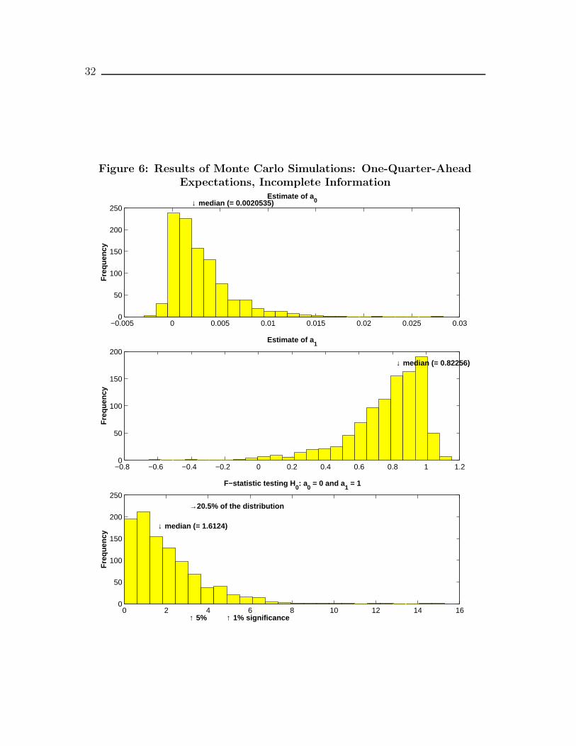
32

Figure 6: Results of Monte Carlo Simulations: One-Quarter-AheadExpectations, Incomplete Information

−0.005 0 0.005 0.01 0.015 0.02 0.025 0.030

50

100

150

200

250↓ median (= 0.0020535)

Fre

quen

cy

Estimate of a0

−0.8 −0.6 −0.4 −0.2 0 0.2 0.4 0.6 0.8 1 1.20

50

100

150

200

↓ median (= 0.82256)

Fre

quen

cy

Estimate of a1

0 2 4 6 8 10 12 14 160

50

100

150

200

250

↓ median (= 1.6124)

→20.5% of the distribution

↑ 5% ↑ 1% significance

Fre

quen

cy

F−statistic testing H0: a

0 = 0 and a

1 = 1

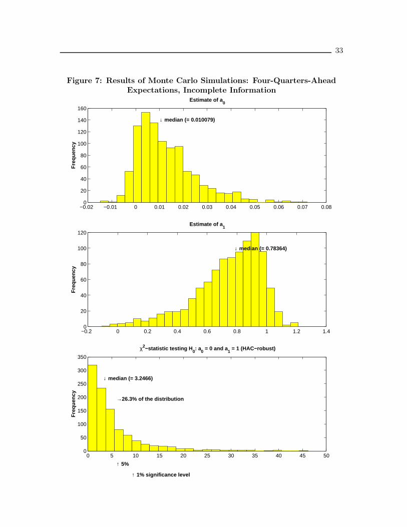
33

Figure 7: Results of Monte Carlo Simulations: Four-Quarters-AheadExpectations, Incomplete Information

−0.02 −0.01 0 0.01 0.02 0.03 0.04 0.05 0.06 0.07 0.080

20

40

60

80

100

120

140

160

↓ median (= 0.010079)

Fre

quen

cy

Estimate of a0

−0.2 0 0.2 0.4 0.6 0.8 1 1.2 1.40

20

40

60

80

100

120

↓ median (= 0.78364)

Fre

quen

cy

Estimate of a1

0 5 10 15 20 25 30 35 40 45 500

50

100

150

200

250

300

350

↓ median (= 3.2466)

→26.3% of the distribution

↑ 5%

↑ 1% significance level

Fre

quen

cy

χ2−statistic testing H0: a

0 = 0 and a

1 = 1 (HAC−robust)

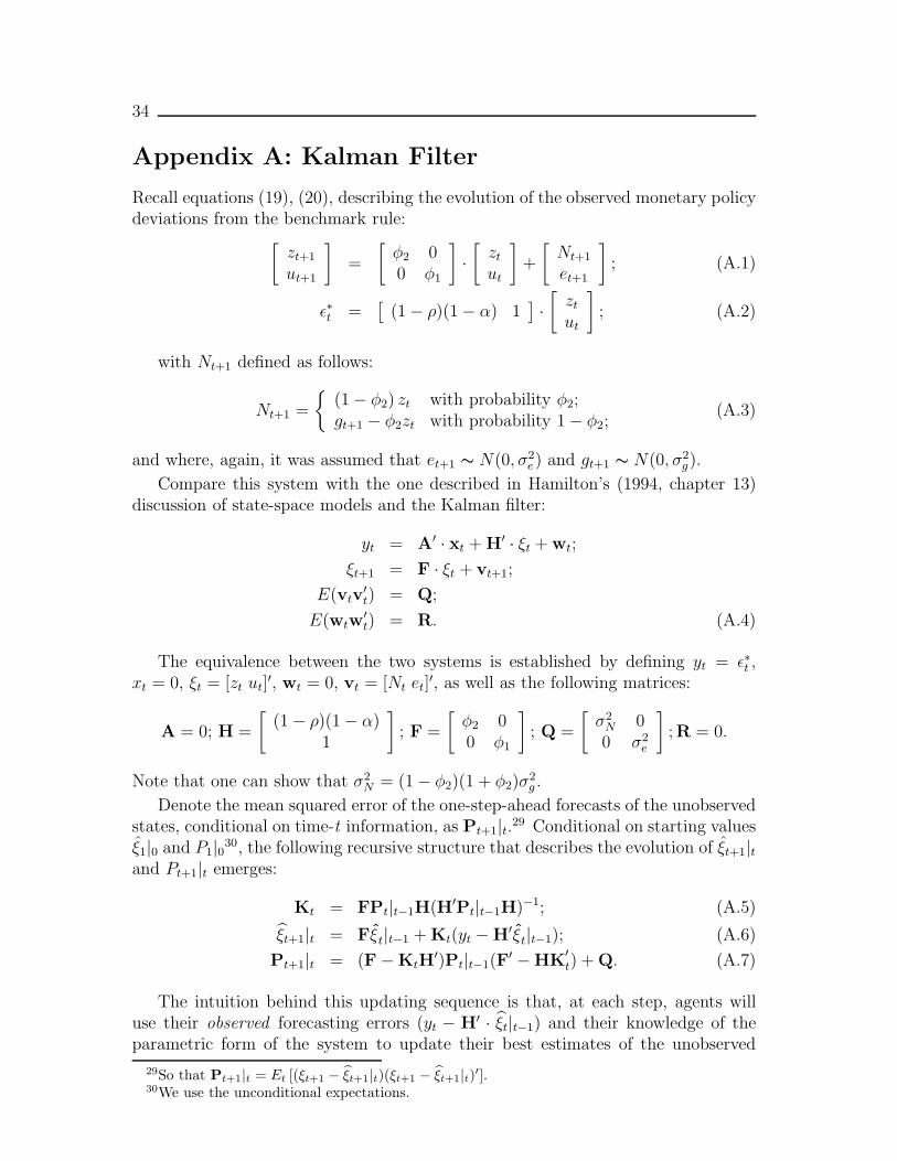
34

Appendix A: Kalman Filter

Recall equations (19), (20), describing the evolution of the observed monetary policydeviations from the benchmark rule:[

zt+1

ut+1

]=

[φ2 00 φ1

]·[ztut

]+

[Nt+1

et+1

]; (A.1)

ε∗t =[

(1 − ρ)(1 − α) 1] · [ zt

ut

]; (A.2)

with Nt+1 defined as follows:

Nt+1 =

{(1 − φ2) zt with probability φ2;gt+1 − φ2zt with probability 1 − φ2;

(A.3)

and where, again, it was assumed that et+1 ∼ N(0, σ2e) and gt+1 ∼ N(0, σ2

g).

Compare this system with the one described in Hamilton’s (1994, chapter 13)discussion of state-space models and the Kalman filter:

yt = A′ · xt + H′ · ξt + wt;

ξt+1 = F · ξt + vt+1;

E(vtv′t) = Q;

E(wtw′t) = R. (A.4)

The equivalence between the two systems is established by defining yt = ε∗t ,xt = 0, ξt = [zt ut]

′, wt = 0, vt = [Nt et]′, as well as the following matrices:

A = 0; H =

[(1 − ρ)(1 − α)

1

]; F =

[φ2 00 φ1

]; Q =

[σ2N 00 σ2

e

];R = 0.

Note that one can show that σ2N = (1 − φ2)(1 + φ2)σ

2g .

Denote the mean squared error of the one-step-ahead forecasts of the unobservedstates, conditional on time-t information, as Pt+1|t.29 Conditional on starting valuesξ1|0 and P1|030, the following recursive structure that describes the evolution of ξt+1|tand Pt+1|t emerges:

Kt = FPt|t−1H(H′Pt|t−1H)−1; (A.5)

ξt+1|t = Fξt|t−1 + Kt(yt − H′ξt|t−1); (A.6)

Pt+1|t = (F − KtH′)Pt|t−1(F

′ − HK′t) + Q. (A.7)

The intuition behind this updating sequence is that, at each step, agents willuse their observed forecasting errors (yt − H′ · ξt|t−1) and their knowledge of theparametric form of the system to update their best estimates of the unobserved

29So that Pt+1|t = Et [(ξt+1 − ξt+1|t)(ξt+1 − ξt+1|t)′].30We use the unconditional expectations.

35

states, ξt. The mechanics of this updating take the form of linear projection and aredetailed in Hamilton.

Under the assumption of normality of both processes (for zt and ut), the se-

quence (ξt+1|t)|Tt=1 represents the optimal one-step-ahead forecasts of the unobservedstates.31

31Even without the assumption of normality, the sequence of filtered estimates remains the bestlinear forecasts of the unobserved states conditional on time-t information.

Bank of Canada Working PapersDocuments de travail de la Banque du Canada

Working papers are generally published in the language of the author, with an abstract in both officiallanguages.Les documents de travail sont publiés généralement dans la langue utilisée par les auteurs; ils sontcependant précédés d’un résumé bilingue.

Copies and a complete list of working papers are available from:Pour obtenir des exemplaires et une liste complète des documents de travail, prière de s’adresser à:

Publications Distribution, Bank of Canada Diffusion des publications, Banque du Canada234 Wellington Street, Ottawa, Ontario K1A 0G9 234, rue Wellington, Ottawa (Ontario) K1A 0G9E-mail: publications@bankofcanada.ca Adresse électronique : publications@banqueducanada.caWeb site: http://www.bankofcanada.ca Site Web : http://www.banqueducanada.ca

20022002-29 Exponentials, Polynomials, and Fourier Series:

More Yield Curve Modelling at the Bank of Canada D.J. Bolder and S. Gusba

2002-28 Filtering for Current Analysis S. van Norden

2002-27 Habit Formation and the Persistenceof Monetary Shocks H. Bouakez, E. Cardia, and F.J. Ruge-Murcia

2002-26 Nominal Rigidity, Desired Markup Variations, andReal Exchange Rate Persistence H. Bouakez

2002-25 Nominal Rigidities and Monetary Policy in CanadaSince 1981 A. Dib

2002-24 Financial Structure and Economic Growth: A Non-Technical Survey V. Dolar and C. Meh

2002-23 How to Improve Inflation Targeting at the Bank of Canada N. Rowe

2002-22 The Usefulness of Consumer Confidence Indexes in theUnited States B. Desroches and M-A. Gosselin

2002-21 Entrepreneurial Risk, Credit Constraints, and the CorporateIncome Tax: A Quantitative Exploration C.A. Meh

2002-20 Evaluating the Quarterly Projection Model: A Preliminary R. Amano, K. McPhail, H. Pioro,Investigation and A. Rennison

2002-19 Estimates of the Sticky-Information Phillips Curvefor the United States, Canada, and the United Kingdom H. Khan and Z. Zhu

2002-18 Estimated DGE Models and Forecasting Accuracy:A Preliminary Investigation with Canadian Data K. Moran and V. Dolar

2002-17 Does Exchange Rate Policy Matter for Growth? J. Bailliu, R. Lafrance, and J.-F. Perrault

2002-16 A Market Microstructure Analysis of Foreign ExchangeIntervention in Canada C. D’Souza

2002-15 Corporate Bond Spreads and the Business Cycle Z. Zhang

2002-14 Entrepreneurship, Inequality, and Taxation C.A. Meh