Embed Size (px)
Citation preview
A Monetary System of Equations with Inflationary Expectations for the U.S.A.
D.S. Bywaters and D.G. Thomas
May 2009 University of Hertfordshire Business School Working Papers are available for download from https://uhra.herts.ac.uk/dspace/handle/2299/619 The Working Paper Series is intended for rapid dissemination of research results, work-in-progress, and innovative teaching methods, at the pre-publication stage. Comments are welcomed and should be addressed to the individual author(s). It should be remembered that papers in this series are often provisional and comments and/or citations should take account of this.
Copyright and all rights therein are retained by authors. All persons copying this information are expected to adhere to the terms and conditions invoked by each
author's copyright. These works may not be re-posted without the explicit permission of the copyright holders.
The Business School at the University of Hertfordshire (UH) employs approximately 150 academic staff in a state-of-the-art environment located in Hatfield Business Park. It offers 17 undergraduate degree programmes, 21 postgraduate programmes and there are about 80 research students, mostly working at doctoral level. Business School staff are active in research in numerous areas, including complexity theory, institutional economics, economic modelling, efficiency measurement the creative industries, employment studies, finance, accounting, statistical methods and management science. The University of Hertfordshire has been recognised as the exemplar of a business-facing university. It is one of the region’s largest employers with over 2,700 staff and a turnover of £205 m. In the 2008 UK Research Assessment Exercise it was given the highest rank for research quality among the post-1992 universities.
1
Abstract: The paper is an empirical investigation that places Livingston’s expectations of the
Consumer Price Index (CPI) with the rate of inflation centre stage in a monetary
system of equations with real money balances, output, employment, Federal
Government debt and interest rates. The modelling approach is a Vector Auto-
Regressions (VARs) scheme employing quarterly, observational data sets from
U.S.A, spanning the period of 1959 to 2007. One of the important tasks is to find
stationary processes for the CPI and the price expectations, which entails explaining
the second-differences within the error-corrections, and using first-differences in
the formation of co-integrating vectors, because the agents view them as levels in
the long-run.
By: Bywaters, D. S. and Thomas, D.G. J.E.L.Classification: C50, D84, E31, E40, H63 Key words: Expectations, Inflation, Money. University of Hertfordshire, Business School, de Havilland Campus, Hatfield, AL10 9AB, England, U.K. E-Mail Address: [email protected]
2
Introduction1 Individual agents in an economy interact with each other in conditions of uncertainty, leading to
the desirability of forming explicit expectations about inflation based on the Consumer Price
Index (CPI). In this empirical investigation, expectations are derived from the Livingston
Survey, started in 1947 (see Appendix A). The analysis entails transforming the observations
into meaningful, quarterly estimates, although the raw data are from half-yearly surveys.
In a number of studies, such as Morana and Bagliano (2007),2 there has been a neglect of
expectations, as well as modelling the chosen price index (or its logarithm) in the light of the
first-difference, which is not necessarily a stationary process. The empirical evidence presented
in this research study, however, suggests that agents view expectations and the rate of inflation -
the first-difference of the logarithm of the price index - as level variables in the long-run
equilibrium process. The stationary tests imply that the second-differences are the correct
variables that require modelling in the overall system of error-corrections. These encapsulate the
short-run dynamics of the variables of interest in the system, which are the deviations from
equilibrium (Enders, 2004).
An important part of the empirical analysis borrows concepts from the Swedish economist, Knut
Wicksell (1936). His theoretical work emphasised the balance between the “market” and the
“natural” rates of interest for equilibrium in an economy. This balance involves both inflation
and expectations, because the “natural rate” is essentially a real variable, whereas the “market
rate” is nominal. This study makes the assumption that Wicksell’s “market” and “natural” rates
1 The writers would like to thank Dr. Tim Parke and Dr. Chris Tofallis for their helpful comments on the drafting of
the paper. 2 Another recent study by De Grauwe and Polan (2005) adopts a similar approach, but neglects many important
variables.
3
of interest involve short-term as well as long-term rates interacting with inflation and
expectations.
The system involves the demand and supply of money and Federal Government debt deflated by
the CPI as well as real income, output and employment, which hopefully forms important
information from the product side of the economy. The employment variable is included on
account of the relationship to the rate of unemployment, and therefore reflects the level of
uncertainty in the formation of expectations in the economy.
The plan of the discussion, then, is to first outline the theoretical model of expectations. Second,
to present the general econometric framework of the VARs system. Third, to define the
variables embodied in the vectors of interest and discuss the data sets involved in the empirical
analysis. Fourth, to present the statistical results relating to the long-run co-integrating
mechanisms: the indicated number of vectors, the results of their estimation and possible
solutions calculated from them. Fifth, various general error correction equations are subjected to
‘Hendryfication’ in order to derive the specific models. Those insignificant quantities that have
no statistical contribution to make in the overall empirical picture are removed, leaving the
significant elements of the short-run dynamics and the equilibrating co-integrating vectors. The
empirical analysis is undertaken using Microfit Econometric Software.
4
The Theoretical Model
The theoretical starting point is with Keynes (1936), who depicts the significance of
expectations and their unstable nature within the economy. His theoretical analyses of the level
of employment, the demand for money, the level of capital expenditure and the trade cycle all
depend crucially on expectations. For instance, in analysing the determination of the level of
employment, Keynes wrote:
Thus the behaviour of each individual firm in deciding its daily output will be determined by its
short-run expectations – expectations as to the cost of output on the various possible scales and
expectations as to the sale-proceeds of this output…..It is upon these various expectations that
the amount of employment which the firms offer will depend. The actually realised results of the
production and scale of output will only be relevant to employment in so far as they cause a
modification of subsequent expectations (Keynes, 1936, p.47).
The difficulty is that he treats expectations as exogenous, which means they are outside of the
model and then cannot be determined by the mechanism of the theory. This is, however, an
erroneous assumption, because expectations in the first instance are perceived as a qualitative
entity, evolving from the inter-play of short-run dynamics, and arising from the imperfect
information, knowledge and complexity that flows from disequilibrium of variables within the
macro economy. Thus the formation of expectations is qualitative in nature, but this fact does
not mean they cannot be endogenized within the edifice of the model, or transformed into
quantitative constructs for analysis (Thomas, 1995).
5
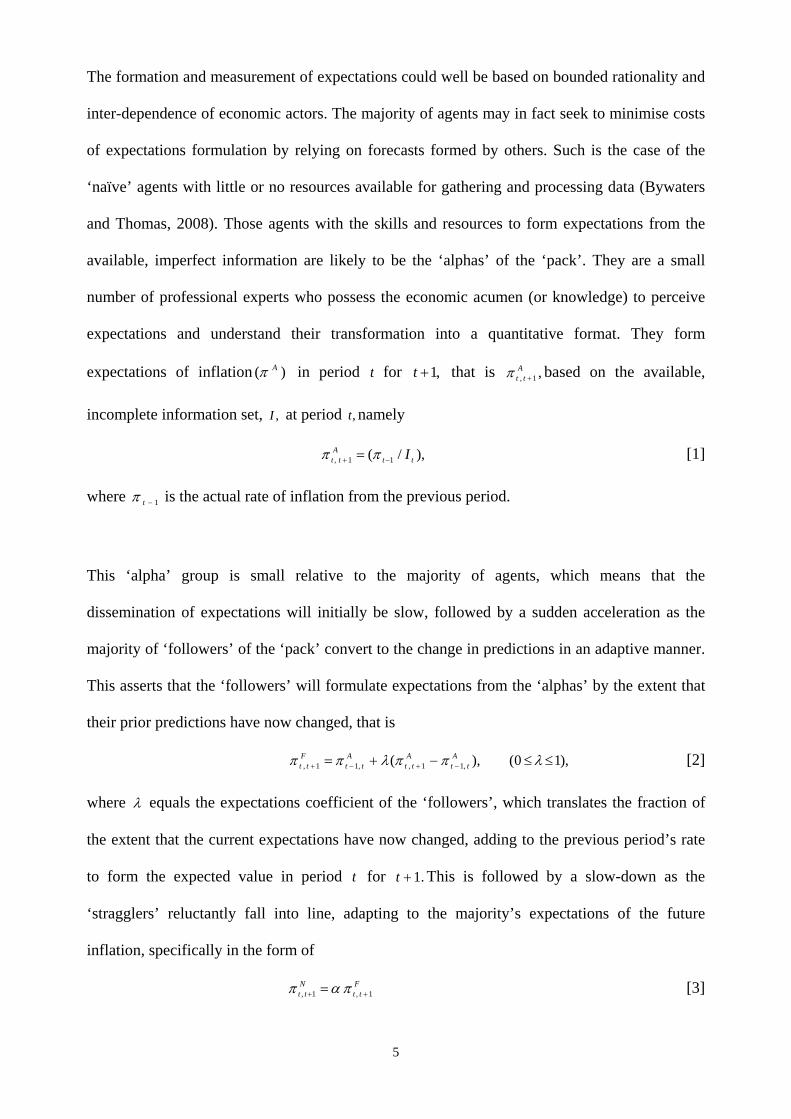
The formation and measurement of expectations could well be based on bounded rationality and
inter-dependence of economic actors. The majority of agents may in fact seek to minimise costs
of expectations formulation by relying on forecasts formed by others. Such is the case of the
‘naïve’ agents with little or no resources available for gathering and processing data (Bywaters
and Thomas, 2008). Those agents with the skills and resources to form expectations from the
available, imperfect information are likely to be the ‘alphas’ of the ‘pack’. They are a small
number of professional experts who possess the economic acumen (or knowledge) to perceive
expectations and understand their transformation into a quantitative format. They form
expectations of inflation )( Aπ in period t for ,1+t that is ,1,A
tt +π based on the available,
incomplete information set, ,I at period ,t namely
),/( 11, ttA
tt I−+ = ππ [1]
where 1−tπ is the actual rate of inflation from the previous period.
This ‘alpha’ group is small relative to the majority of agents, which means that the
dissemination of expectations will initially be slow, followed by a sudden acceleration as the
majority of ‘followers’ of the ‘pack’ convert to the change in predictions in an adaptive manner.
This asserts that the ‘followers’ will formulate expectations from the ‘alphas’ by the extent that
their prior predictions have now changed, that is
),10(),( ,11,,11, ≤≤−+= −+−+ λππλππ Att
Att
Att
Ftt [2]
where λ equals the expectations coefficient of the ‘followers’, which translates the fraction of
the extent that the current expectations have now changed, adding to the previous period’s rate
to form the expected value in period t for .1+t This is followed by a slow-down as the
‘stragglers’ reluctantly fall into line, adapting to the majority’s expectations of the future
inflation, specifically in the form of
Ftt
Ntt 1,1, ++ = παπ [3]
6
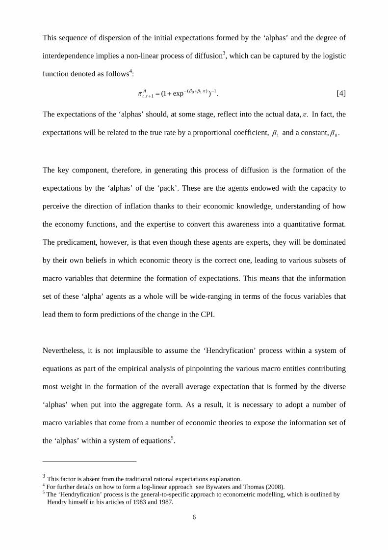
This sequence of dispersion of the initial expectations formed by the ‘alphas’ and the degree of
interdependence implies a non-linear process of diffusion3, which can be captured by the logistic
function denoted as follows4:
.)exp1( 1)(1,
10 −+−+ += πββπ A
tt [4]
The expectations of the ‘alphas’ should, at some stage, reflect into the actual data, .π In fact, the
expectations will be related to the true rate by a proportional coefficient, 1β and a constant, .0β
The key component, therefore, in generating this process of diffusion is the formation of the
expectations by the ‘alphas’ of the ‘pack’. These are the agents endowed with the capacity to
perceive the direction of inflation thanks to their economic knowledge, understanding of how
the economy functions, and the expertise to convert this awareness into a quantitative format.
The predicament, however, is that even though these agents are experts, they will be dominated
by their own beliefs in which economic theory is the correct one, leading to various subsets of
macro variables that determine the formation of expectations. This means that the information
set of these ‘alpha’ agents as a whole will be wide-ranging in terms of the focus variables that
lead them to form predictions of the change in the CPI.
Nevertheless, it is not implausible to assume the ‘Hendryfication’ process within a system of
equations as part of the empirical analysis of pinpointing the various macro entities contributing
most weight in the formation of the overall average expectation that is formed by the diverse
‘alphas’ when put into the aggregate form. As a result, it is necessary to adopt a number of
macro variables that come from a number of economic theories to expose the information set of
the ‘alphas’ within a system of equations5.
3 This factor is absent from the traditional rational expectations explanation. 4 For further details on how to form a log-linear approach see Bywaters and Thomas (2008). 5 The ‘Hendryfication’ process is the general-to-specific approach to econometric modelling, which is outlined by
Hendry himself in his articles of 1983 and 1987.
7
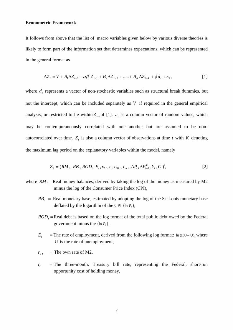
Econometric Framework
It follows from above that the list of macro variables given below by various diverse theories is
likely to form part of the information set that determines expectations, which can be represented
in the general format as
,.....221'
11 ttktKtttt dZBZBZZBVZ εφαβ ++Δ++Δ++Δ+=Δ −−−− [1]
where td represents a vector of non-stochastic variables such as structural break dummies, but
not the intercept, which can be included separately as V if required in the general empirical
analysis, or restricted to lie within 1−tZ of [1]. tε is a column vector of random values, which
may be contemporaneously correlated with one another but are assumed to be non-
autocorrelated over time. tZ is also a column vector of observations at time t with K denoting
the maximum lag period on the explanatory variables within the model, namely
,),,,,,,,,,,,( 1302 ′ΔΔ= + CYPPrrrrERGDRBRMZ tE
tttmtttttttt [2]
where tRM = Real money balances, derived by taking the log of the money as measured by M2 minus the log of the Consumer Price Index (CPI),
=tRB Real monetary base, estimated by adopting the log of the St. Louis monetary base deflated by the logarithm of the CPI ( )tPln ,
=tRGD Real debt is based on the log format of the total public debt owed by the Federal government minus the ( )tPln ,
=tE The rate of employment, derived from the following log format: U),100(ln − where U is the rate of unemployment,
=tr2 The own rate of M2,
=tr The three-month, Treasury bill rate, representing the Federal, short-run opportunity cost of holding money,
8
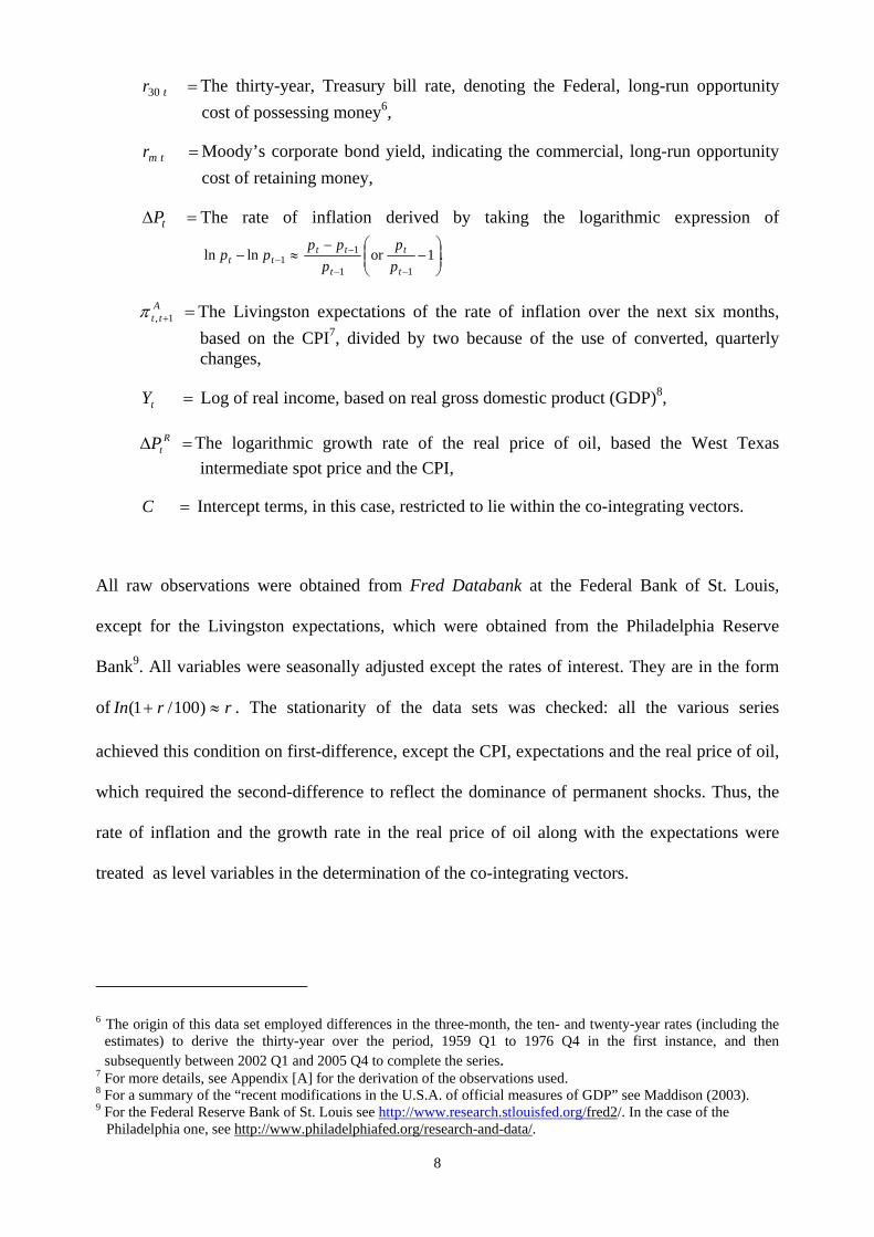
=tr30 The thirty-year, Treasury bill rate, denoting the Federal, long-run opportunity cost of possessing money6,
=tmr Moody’s corporate bond yield, indicating the commercial, long-run opportunity cost of retaining money,
=Δ tP The rate of inflation derived by taking the logarithmic expression of
.1orlnln11
11 ⎟⎟
⎠
⎞⎜⎜⎝
⎛−
−≈−
−−
−−
t
t
t
tttt p
pp
pppp
=+A
tt 1,π The Livingston expectations of the rate of inflation over the next six months, based on the CPI7, divided by two because of the use of converted, quarterly changes,
=tY Log of real income, based on real gross domestic product (GDP)8,
=Δ RtP The logarithmic growth rate of the real price of oil, based the West Texas
intermediate spot price and the CPI,
=C Intercept terms, in this case, restricted to lie within the co-integrating vectors.
All raw observations were obtained from Fred Databank at the Federal Bank of St. Louis,
except for the Livingston expectations, which were obtained from the Philadelphia Reserve
Bank9. All variables were seasonally adjusted except the rates of interest. They are in the form
of rrIn ≈+ )100/1( . The stationarity of the data sets was checked: all the various series
achieved this condition on first-difference, except the CPI, expectations and the real price of oil,
which required the second-difference to reflect the dominance of permanent shocks. Thus, the
rate of inflation and the growth rate in the real price of oil along with the expectations were
treated as level variables in the determination of the co-integrating vectors.
6 The origin of this data set employed differences in the three-month, the ten- and twenty-year rates (including the
estimates) to derive the thirty-year over the period, 1959 Q1 to 1976 Q4 in the first instance, and then subsequently between 2002 Q1 and 2005 Q4 to complete the series.
7 For more details, see Appendix [A] for the derivation of the observations used. 8 For a summary of the “recent modifications in the U.S.A. of official measures of GDP” see Maddison (2003). 9 For the Federal Reserve Bank of St. Louis see http://www.research.stlouisfed.org/fred2/. In the case of the
Philadelphia one, see http://www.philadelphiafed.org/research-and-data/.
9
The next stage in the empirical analysis was to determine the number of co-integrating vectors
existing between the non-stationary variables of interest in ,1−′ tZβα representing the long-run
equilibria. The number of different co-integrating vectors can be found by examining the
significance of the characteristic roots, which is the rank of a matrix (Johansen, 1988; Stock and
Watson, 1988). The tests for the total number of roots that are significantly different from one
use the maximum and trace statistics. The results of the maximum and trace statistics give
conflicting measures, although the former rather than the latter have the sharper alternative
hypothesis, and are therefore, the preferred statistic when trying to discover the number of co-
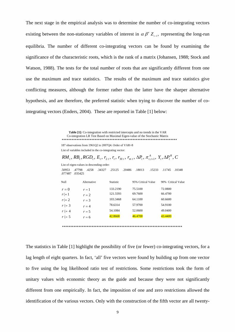
integrating vectors (Enders, 2004). These are reported in Table [1] below:
Table [1]: Co-integration with restricted intercepts and no trends in the VAR Co-integration LR Test Based on Maximal Eigen-value of the Stochastic Matrix
**********************************************************************
187 observations from 1961Q2 to 2007Q4. Order of VAR=8
List of variables included in the co-integrating vector:
CPYPrrrrERGDRBRM Rtt
Attttmttttttt ,,,,,,,,,,,, 1,302 ΔΔ +π
List of eigen-values in descending order:
.50953 .47798 .4258 .34327 .25125 .20486 .18013 .15233 .11745 .10348
.077487 .035425
Null Alternative Statistic 95% Critical Value 90% Critical Value
0=r 1=r 133.2190 75.5100 72.0800
1⟨=r 2=r 121.5593 69.7600 66.4700
2⟨=r 3=r 103.3468 64.1100 60.6600 3⟨=r 4=r 78.6314 57.9700 54.9100
4⟨=r 5=r 54.1084 52.0600 49.0400
5⟨=r 6=r 42.8668 46.4700 43.4400
*************************************************************************
The statistics in Table [1] highlight the possibility of five (or fewer) co-integrating vectors, for a
lag length of eight quarters. In fact, ‘all’ five vectors were found by building up from one vector
to five using the log likelihood ratio test of restrictions. Some restrictions took the form of
unitary values with economic theory as the guide and because they were not significantly
different from one empirically. In fact, the imposition of one and zero restrictions allowed the
identification of the various vectors. Only with the construction of the fifth vector are all twenty-
10
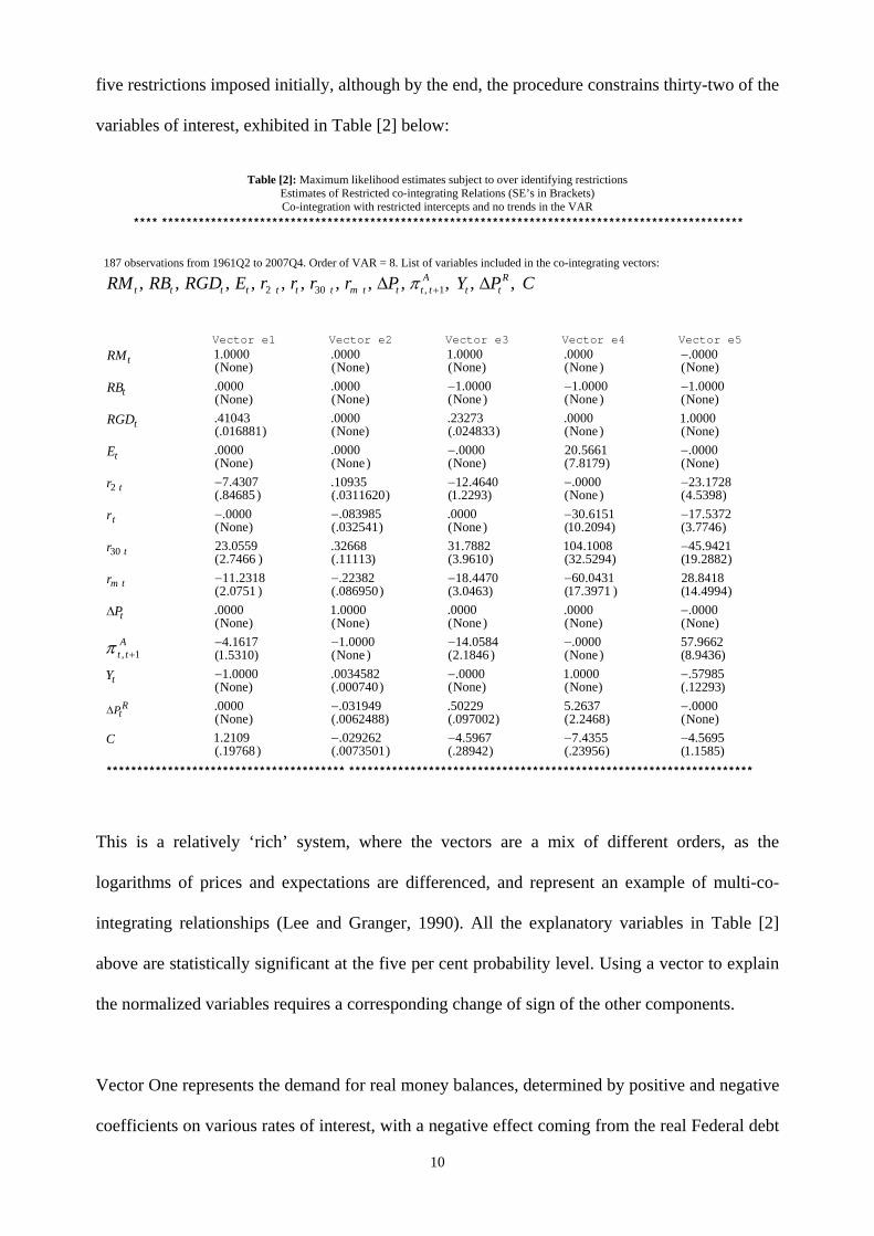
five restrictions imposed initially, although by the end, the procedure constrains thirty-two of the
variables of interest, exhibited in Table [2] below:
Table [2]: Maximum likelihood estimates subject to over identifying restrictions Estimates of Restricted co-integrating Relations (SE’s in Brackets) Co-integration with restricted intercepts and no trends in the VAR
**** *********************************************************************************************** 187 observations from 1961Q2 to 2007Q4. Order of VAR = 8. List of variables included in the co-integrating vectors:
CPYPrrrrERGDRBRM Rtt
Attttmttttttt ,,,,,,,,,,,, 1,302 ΔΔ +π
Vector e1 Vector e2 Vector e3 Vector e4 Vector e5
tRM )None(
0000.1 )None(0000. )None(
0000.1 )None(0000. )None(
0000.−
tRB )None(
0000. )None(0000. )None(
0000.1− )None(0000.1− )None(
0000.1−
tRGD )016881(.
41043. )None(0000. )024833(.
23273. )None(0000. )None(
0000.1
tE )None(
0000. )None(0000. )None(
0000.− )8179.7(5661.20 )None(
0000.−
tr2 )84685(.
4307.7− )0311620(.10935. )2293.1(
4640.12− )None(0000.− )5398.4(
1728.23−
tr )None(
0000.− )032541(.083985.− )None(
0000. )2094.10(6151.30− )7746.3(
5372.17−
tr30 )7466.2(
0559.23 )11113(.32668. )9610.3(
7882.31 )5294.32(1008.104 )2882.19(
9421.45−
tmr )0751.2(
2318.11− )086950(.22382.− )0463.3(
4470.18− )3971.17(0431.60− )4994.14(
8418.28
tPΔ )None(
0000. )None(0000.1 )None(
0000. )None(0000. )None(
0000.−
Att 1, +π )5310.1(
1617.4− )None(0000.1− )1846.2(
0584.14− )None(0000.− )9436.8(
9662.57
tY )None(
0000.1− )000740(.0034582. )None(
0000.− )None(0000.1 )12293(.
57985.−
RtPΔ
)None(0000. )0062488(.
031949.− )097002(.50229. )2468.2(
2637.5 )None(0000.−
C )19768(.
2109.1 )0073501(.029262.− )28942(.
5967.4− )23956(.4355.7− )1585.1(
5695.4−
*************************************** ******************************************************************
This is a relatively ‘rich’ system, where the vectors are a mix of different orders, as the
logarithms of prices and expectations are differenced, and represent an example of multi-co-
integrating relationships (Lee and Granger, 1990). All the explanatory variables in Table [2]
above are statistically significant at the five per cent probability level. Using a vector to explain
the normalized variables requires a corresponding change of sign of the other components.
Vector One represents the demand for real money balances, determined by positive and negative
coefficients on various rates of interest, with a negative effect coming from the real Federal debt
11
along with the positive signs on the output/income and the expectations variables. The positive
coefficient on expectations means that agents are preserving the purchasing-power of their
money holdings at the expense of other financial assets within their portfolio choices. The
textbook answer would suggest that if the ability to spend money balances is being eroded away
in the future, then households would reduce holdings by purchasing more goods and services.
In the case of the debt, there is an inverse relationship because borrowing by the Authorities,
which represents a rise in the Federal holdings of money to finance Government expenditure,
and therefore, reduces real money balances held by the Public on account of the purchase.
Vector Two is the long-run information set of expectations and the rate of inflation of equation
[1], which seems to be in the world of Wicksell (1936)10, where the economy’s expectations and
the rate of inflation are stabilized by the ‘balance’ of rates of interest, output and the real oil
price. The three-month and the corporate rates of interest indicate positive relationships between
the rate of inflation and expectations. When inflation is rising with expectations, there is
tightening of monetary policy, which results in the short-run rate of interest going up as part of
the “damping-process”. This process with the term-structure forces the thirty-year rate of
interest upwards, which proxies and reflects the “natural rate” with a negative relationship in the
‘Wicksellian’ equilibrium on account of the imposition of indirect effects on the rate of
investment expenditure, and therefore, the economy’s output11. In other words, as the long-run
(or “natural”) rate of interest rises, reducing capital expenditure, and consequently, aggregate
demand, which in turn pulls down the rate of growth in prices with expectations. Clearly, a
definite link can be seen between the “natural” and “market” rates of interest, the rate of
inflation and expectations. The ‘own’ rate of interest seems to be playing a similar part in the
process of development, through this links with the real demand for money.
10 Also see Woodford (2003) for a discussion of the links to monetary policy. 11 In Keynes’s analysis (1936), it is the marginal efficiency of capital determining the rate of capital accumulation
and the change in the level of aggregate demand and supply.
12
On the question of inflation and expectations, twin monetary forces are brought into play to
explain the indirect effects on the level of economic activity. In the language of Wicksell, this is
a “cumulative process” of falling activity12. This process also affects the aggregate supply side
of the economy, where the cumulative process in terms of less output forces the rate of inflation
and expectations down, as a result of the increase in the “natural rate” of interest reducing
growth in the long run.
A further noticeable feature in Vector Two is the approximate one-to-one rate of inflation with
the expectations variable, the so-called “unitary elasticity of expectations” in Hick’s
terminology (Blaug, 1997). This means that an alteration in existing prices is predicted to
change future ones in the equivalent direction, and to tend towards the identical proportion from
any disturbance from equilibrium, such that the ‘cumulative process generates its own breeze’.
Thus, individuals expect the change in prices to rise as fast as present ones (Hicks, 1968). This
is Popper’s prophecy of self-fulfilling expectations, dubbed by him the “Oedipus effect”
(Popper, 1970).
The argument above suggests a weak form of rational expectations may exist in the long run
based on bounded rationality. This might be a reasonable assumption given that the agents in the
Livingston Survey, the so-called ‘alphas’ of the ‘pack’ (Bywaters and Thomas, 2008), are
aware, to some degree, of the underlying economic factors that generate future inflation, and
use, where possible, all the available information in the determination of forecasts of key
variables. Furthermore, if the actual and expected inflation rates are roughly equal, this implies
equality between the real and the potential output, given the theoretical debate. The difficulty for
12 In the analysis of Keynes, it is the multiplier effect of output rather than prices, which is treated as fixed because
the analysis is set in a picture of idle resources (Blaug, 1997).
13
the empirical analysis is that the latter are trended variables whereas the former are not, and
therefore only actual output is a necessary condition in the estimation of the system. Briefly,
when sewn together, all the threads indicate an ‘augmented Wicksell curve’, that is the rate of
inflation is determined by expectations and shifted by twin forces of short- and long-run (or
“natural”) rates of interest, directing the cumulative process of investment and output that lies
backstage.
Vector Three is the supply of real money, driven by the plus one coefficient on the real
monetary base, the reverse value on real Government debt, various interest rates with differing
signs, but a positive rôle for expectations and a negative part for the rate growth in the real price
of oil. It represents a key vector in the overall stabilization policy of the system because it
encapsulates the rôle of expectations, the real monetary base and the Federal debt. Whereas the
latter variables are largely under the control of the monetary authorities, the former is
determined by the ‘alphas’.
Vector Four determines real output as the real monetary base. Assuming the latter rather than
the former, employment and real output will have similar effects. There is a mix of effects
coming through from the rates of interest with an expected, negative value on the rate of growth
of the real price of oil. Clearly, given the various rates of interest, the effect on output does not
always show the likely crowding-out effect.
The Final Vector in the system is the supply of bonds in real terms emanating from the real debt
issued by the Federal Authorities to the Public on behalf of the Government. The coefficient of
plus one on real high-powered money represents the debt sold to itself in order to monetize the
effect on interest rates, but leading to the creation of new money. The selling of debt to the
Public, however, leads to a positive effect on the thirty-year Treasury bill rate, suggesting the
14
possibility of crowding-out in the long-run, but the opposite value coming from the Corporate
Yield. The overall end-result of the two forms of debt financing is the positive effect with
income. The short-run rate of interest exhibits a negative coefficient, whereas the own rate on
M2 is positive. Finally, the negative coefficient on the expectations variable suggests that the
real burden of Federal debt created by the state will be reduced in the long-run.
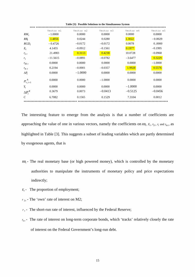
The next part of the procedure is to derive a possible solution to the simultaneous equation
system by taking linear combinations with algebra of the five estimated vectors in Table [2].
This is done by vector space column operations, either multiplying a vector by a factor κ or by
adding (or subtracting) another one. This practice is analogous to changing co-ordinates in
geometry, leaving the basic structure unchanged. The solution for the following subset of
‘focus’ variables: tA
ttttt YPrRM and,,, 1,30 +Δ π chosen on theoretical grounds as
relatively endogenous, is shown in Table [3] overleaf.
These variables above are set equal to zero in the five vectors except in the case of the
normalization, chosen to be minus one so that the other coefficients have the correct sign. For
instance, in the first case, the tRM in Vector one is the normalised variable with the other ‘focus’
variables set equal to zero; the second case, tr30 in Vector two is normalised, with
tA
tttt YPRM and,,, 1, +Δ π put to zero. The procedure continues until the end-variable of
tY with Attttt PrRM 1,30 and,,, +Δ π equalling zero. The calculated coefficients in Table [3]
can then be directly compared with theory because the normalizations are in terms of -1.
15
Table [3]: Possible Solutions to the Simultaneous System **** ***********************************************************************************************
Vector e1 Vector e2 Vector e3 Vector e4 Vector e5
tRM 0000.1− 0000.0 0000.0 0000.0 0000.0
tRB 4856.1 0244.0 0280.0 3022.1 0029.0−
tRGD 4726.0− 0172.0− 0172.0− 0078.0 0000..0
tE 1455.4 0912.0− 1561.0− 1977.0 1995.0−
tr2 4983.21 3113.0 4238.0 0728.10 0968.0−
tr 5615.11− 0891.0− 0782.0− 6477.3− 3229.0
tr30 0000.0 0000.0 0000.0 0000.0 0000.1−
tmr 2194.0 0001.0− 0357.0− 9928.1 5576.0
tPΔ 0000.0 0000.1− 0000.0 0000.0 0000.0
Att 1, +π 0000.0 0000.0 0000.1− 0000.0 0000.0
tY 0000.0 0000.0 0000.0 0000.1− 0000.0
RtPΔ 3679.0 0073.0 0413.0− 5125.0− 0456.0−
C 7082.6 1565.0 1529.0 3104.7 0012.0
*************************************** ******************************************************************
The interesting feature to emerge from the analysis is that a number of coefficients are
approaching the value of one in various vectors, namely the coefficients on ,rand,,, tm2 tttt rrERB as
highlighted in Table [3]. This suggests a subset of leading variables which are partly determined
by exogenous agents, that is
tRB - The real monetary base (or high powered money), which is controlled by the monetary
authorities to manipulate the instruments of monetary policy and price expectations
indirectly;
tE - The proportion of employment;
tr 2 - The ‘own’ rate of interest on M2;
tr - The short-run rate of interest, influenced by the Federal Reserve;
tmr - The rate of interest on long-term corporate bonds, which ‘tracks’ relatively closely the rate
of interest on the Federal Government’s long-run debt.
16
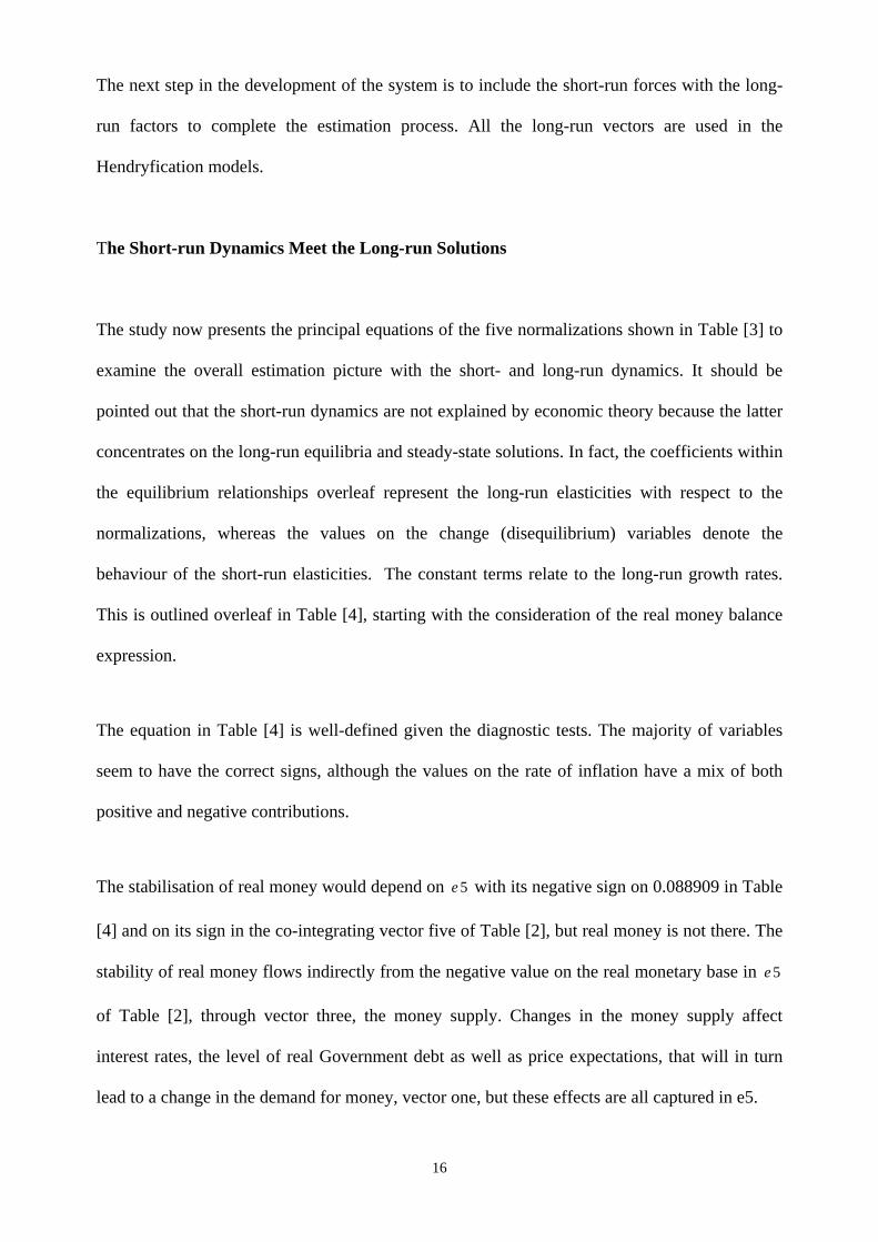
The next step in the development of the system is to include the short-run forces with the long-
run factors to complete the estimation process. All the long-run vectors are used in the
Hendryfication models.
The Short-run Dynamics Meet the Long-run Solutions
The study now presents the principal equations of the five normalizations shown in Table [3] to
examine the overall estimation picture with the short- and long-run dynamics. It should be
pointed out that the short-run dynamics are not explained by economic theory because the latter
concentrates on the long-run equilibria and steady-state solutions. In fact, the coefficients within
the equilibrium relationships overleaf represent the long-run elasticities with respect to the
normalizations, whereas the values on the change (disequilibrium) variables denote the
behaviour of the short-run elasticities. The constant terms relate to the long-run growth rates.
This is outlined overleaf in Table [4], starting with the consideration of the real money balance
expression.
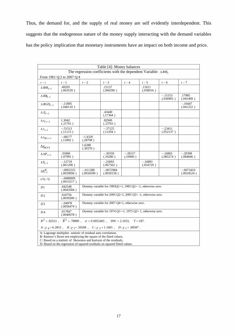
The equation in Table [4] is well-defined given the diagnostic tests. The majority of variables
seem to have the correct signs, although the values on the rate of inflation have a mix of both
positive and negative contributions.
The stabilisation of real money would depend on 5e with its negative sign on 0.088909 in Table
[4] and on its sign in the co-integrating vector five of Table [2], but real money is not there. The
stability of real money flows indirectly from the negative value on the real monetary base in 5e
of Table [2], through vector three, the money supply. Changes in the money supply affect
interest rates, the level of real Government debt as well as price expectations, that will in turn
lead to a change in the demand for money, vector one, but these effects are all captured in e5.
17
Thus, the demand for, and the supply of real money are self evidently interdependent. This
suggests that the endogenous nature of the money supply interacting with the demand variables
has the policy implication that monetary instruments have an impact on both income and price.
Table [4]: Money balances The regression coefficients with the dependent Variable: tRMΔ
From 1961 Q:2 to 2007 Q:4 it − 1−t 2−t 3−t 4−t 5−t 6−t 7−t
itRM −Δ )063539(.
49205. )060290(.15137. )058016(.
11611.
itRB −Δ )036905(.15153.− )041409(.
17985. itRGD −Δ
)046110(.11895.− )041252(.
10447.− itE −Δ )17364(.
43440.
itr −Δ 2 )21761(.
3042.1 )23761(.82949.
itr −Δ )11115(.
51513.− )11294(.37125.− )052137(.
23411.−
itr −Δ 30 )11892(.
68177.− )28708(.4320.1−
itmr −Δ )30376(.6288.1
itP −ΔΔ )07991(.
35968. )10280(.30359.− )10900(.
28157.− )085274(.16865.− )084846(.
20398.− itY −Δ
)061208(.12719.− )067562(.
25093.− )054729(.16891.−
RitP −Δ )0029694(.
0092225.− )0034599(.011288.−
)0030158(.0072984.− )0024524(.
0073410.−
)1(5 −e )0013217(.
0088909.− 1D
)0043584(.042548. Dummy variable for 1983Q1=1, 1983 Q2= -1, otherwise zero.
2D )0039300(.
010756. Dummy variable for 2005 Q2=1, 2005 Q3= -1, otherwise zero.
3D )0056474(.
04978.− Dummy variable for 2007 Q4=1, otherwise zero.
4D )0040078(.
017847. Dummy variable for 1974 Q1=-1, 1975 Q2= 1, otherwise zero.
.89587.:,1601.1:,59268.:,2853.6:A
187.T2.1033,DW,0052465.0,78889.,82521.
1214
22
====
=====
χχχχ
σ
DCB
RR
A: Lagrange multiplier statistic of residual auto correlation, B: Ramsey’s Reset test employing the square of the fitted values, C: Based on a statistic of Skewness and kurtosis of the residuals, D: Based on the regression of squared residuals on squared fitted values.
18
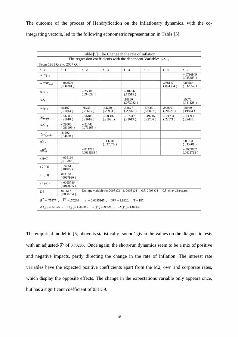
The outcome of the process of Hendryfication on the inflationary dynamics, with the co-
integrating vectors, led to the following econometric representation in Table [5]:
Table [5]: The Change in the rate of Inflation The regression coefficients with the dependent Variable: tPΔΔ
From 1961 Q:2 to 2007 Q:4 it − 1−t 2−t 3−t 4−t 5−t 6−t 7−t
itRB −Δ )035483(.0796949.−
itRGD −Δ )034381(.
083570.− )024354(.086117. )032957(.
085968. itr −Δ 2 )094633(.
25800.− )15515(.48276.−
itr −Δ )073082(.18860. )041128(.
10072. itr −Δ 30
)21044(.95107. )20625(.
78255. )20934(.62250. )20962(.
58627. )20827(.57835. )20728(.
90900. )19874(.69969.
itmr −Δ )21610(.56585.− )21616(.
56185.− )21991(.58886.− )22619(.
57747.− )22706(.49216.− )22371(.
71794.− )22400(.73693.−
itP −ΔΔ )091909(.
29888.− )071165(.21442.−
Aitt −+Δ 1,π )34680(.
81392.
itY −Δ )037576(.13210.− )035901(.
083731. R
itP −Δ )0034599(.011288.− )0015763(.
0039862.−
)1(1 −e )010385(.
036160.− )1(2 −e
)10405(.74651.−
)1(3 −e )0087930(.
024150. )1(4 −e
)0012605(.0055786.−
5D )0030234(.
016617. Dummy variable for 2005 Q3 =1, 2005 Q4 = -0.5, 2006 Q4 = -0.5, otherwise zero.
.0613.1:,99990.:,3480.1:,63627.:A
187.T1.9820,DW,0035165.0,70260.,75377.
1214
22
====
=====
χχχχ
σ
DCB
RR
The empirical model in [5] above is statistically ‘sound’ given the values on the diagnostic tests
with an adjusted- 2R of 0.70260. Once again, the short-run dynamics seem to be a mix of positive
and negative impacts, partly directing the change in the rate of inflation. The interest rate
variables have the expected positive coefficients apart from the M2, own and corporate rates,
which display the opposite effects. The change in the expectations variable only appears once,
but has a significant coefficient of 0.8139.
19
The major, outstanding feature, however, is the significant number of equilibrium mechanisms
being retained by the empirical model, except ,5e which represent a combination of positive and
negative processes forcing the system back on the ‘road of stability’, depending on the quarterly
values embodied in the Vectors over the sample period. It is, however, clear that 2e has the
largest coefficient with a negative sign of 0.74651, giving rise to the most influential of the
equilibrating vectors, which in Table [2] has inflation with a coefficient of plus one.
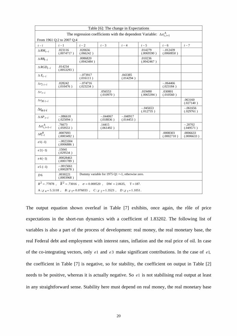
The next equation to view, resulting from the process of Hendryfication, is the particularly
important one of expectations, modelled in Table [6] overleaf, exposing principal parts of the
information set. This is partly determined by the rate of inflation and expectations itself along
with interest rates as well as the following real variables: money, employment, debt, the
monetary base and the price of oil. All the Vectors except ,3e the real money supply, seem to
play significant rôles in the equilibrating process with positive and negative contributions to the
explanation of the dependent variable and driving it to the equilibrium pathway. For instance, in
Vector Two of Table [2], the expectations variable has a negative coefficient. In Table [6] 2e
has a positive coefficient, which is appropriate for determining the stability of expectations. In
short, the diagnostic statistics in [6] seem to indicate a healthy, well-defined econometric model
with an adjusted- 2R of 0.7306, indicating that a significant explanation of the modification
process of the change in expectations of the ‘alphas’, the leaders of the ‘pack’.
20
Table [6]: The change in Expectations
The regression coefficients with the dependent Variable: Att 1, +Δπ
From 1961 Q:2 to 2007 Q:4 it − 1−t 2−t 3−t 4−t 5−t 6−t 7−t
itRM −Δ )0074717(.
023116. )066242(.020656. )0069590(.
014279.)0060850(.
012439.−
itRB −Δ )0042484(.0086820. )0042467(.
010236.
itRGD −Δ )0053293(.
014234.
itE −Δ )016111(.073917.− )014294(.
043385.
itr −Δ 2 )010476(.
028242. )023234(.074716.− )023184(.
064466.−
itr −Δ )010970(.056553. )0065394(.
019490.)010560(.
030801.
itr −Δ 30 )027140(.063160.
itmr −Δ )012735(.045653.− )029761(.
061656.− itP −ΔΔ
)025094(.086618.− )018836(.
044067.− )014453(.040917.−
Aitt −+Δ 1,π )059551(.
76673. )061492(.14415. )049571(.
20702.− R
itP −Δ )0003492(.0007693. )0002710(.
0008303. )0006633(.0006633.
)1(1 −e )0006886(.
0023304.− )1(2 −e
)029534(.15041.
)1(4 −e )0001789(.
00028463. )1(5 −e
)0002878(.0015661.−
6D )0003968(.
0030221. Dummy variable for 1975 Q1 =-1, otherwise zero.
.1051.1:,3523.1:,076033.0:,5118.5:A
187.T2.0635,DW,000520.0,73016.,77878.
1214
22
====
=====
χχχχ
σ
DCB
RR
The output equation shown overleaf in Table [7] exhibits, once again, the rôle of price
expectations in the short-run dynamics with a coefficient of 1.83202. The following list of
variables is also a part of the process of development: real money, the real monetary base, the
real Federal debt and employment with interest rates, inflation and the real price of oil. In case
of the co-integrating vectors, only 1e and 3e make significant contributions. In the case of ,1e
the coefficient in Table [7] is negative, so for stability, the coefficient on output in Table [2]
needs to be positive, whereas it is actually negative. So 1e is not stabilising real output at least
in any straightforward sense. Stability here must depend on real money, the real monetary base
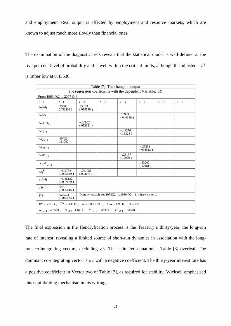
21
and employment. Real output is affected by employment and resource markets, which are
known to adjust much more slowly than financial ones.
The examination of the diagnostic tests reveals that the statistical model is well-defined at the
five per cent level of probability and is well within the critical limits, although the adjusted - 2R
is rather low at 0.43530.
Table [7]: The change in output The regression coefficients with the dependent Variable: tYΔ
From 1961 Q:2 to 2007 Q:4 it − 1−t 2−t 3−t 4−t 5−t 6−t 7−t
itRM −Δ )052401(.
23508. )058589(.27163.
itRB −Δ )040349(.10949.
itRGD −Δ )052381(.10982.−
itE −Δ )13328(.41376.−
itr −Δ 2 )11082(.
60428.
itr −Δ 30 )098512(.26231.−
itP −ΔΔ )10900(.28157.−
Aitt −+Δ 1,π )50281(.
83202.1 R
itP −Δ )0035839(.019754.− )0031770(.
011081.− )1(1 −e
)0097669(.0135122.−
)1(3 −e )0056645(.
044191. 8D
)0045034(.028503. Dummy variable for 1978Q2=1, 1980 Q2= -1, otherwise zero.
.31390.:,65327.:,0712.1:,3538.4:A
187.T1.9534,DW,0061995.0,43530.,47153.
1214
22
====
=====
χχχχ
σ
DCB
RR
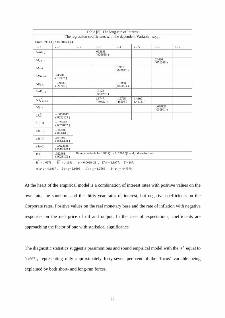
The final expression in the Hendryfication process is the Treasury’s thirty-year, the long-run
rate of interest, revealing a limited source of short-run dynamics in association with the long-
run, co-integrating vectors, excluding .5e The estimated equation is Table [8] overleaf. The
dominant co-integrating vector is ,2e with a negative coefficient. The thirty-year interest rate has
a positive coefficient in Vector two of Table [2], as required for stability. Wicksell emphasised
this equilibrating mechanism in his writings.
22
Table [8]: The long-run of Interest The regression coefficients with the dependent Variable: tr30Δ
From 1961 Q:2 to 2007 Q:4 it − 1−t 2−t 3−t 4−t 5−t 6−t 7−t
itRB −Δ )026628(.053938.
itr −Δ 2 )071348(.24420.
itr −Δ )042971(.13991.
itr −Δ 30 )19307(.
74520.
itmr −Δ )20706(.69883.− )086053(.
18988.−
itP −ΔΔ )048964(.13122.
Aitt −+Δ 1,π )40332(.
5747.1 )48506(.2725.1− )41121(.
4102.1
itY −Δ )036901(.098123.−
RitP −Δ )0023129(.
0050647.− )1(1 −e
)0074067(.028682.−
)1(2 −e )073261(.
16886.− )1(3 −e
)0064468(.021592.
)1(4 −e )0008409(.
0023538.− 7D
)0028102(.022481. Dummy variable for 1980 Q1 = 1, 1980 Q2 = -1, otherwise zero.
.047570.:,3686.1:,9893.2:,1867.4:A
187.T1.8977,DW,0038428.0,41681.,46671.
1214
22
====
=====
χχχχ
σ
DCB
RR
At the heart of the empirical model is a combination of interest rates with positive values on the
own rate, the short-run and the thirty-year rates of interest, but negative coefficients on the
Corporate rates. Positive values on the real monetary base and the rate of inflation with negative
responses on the real price of oil and output. In the case of expectations, coefficients are
approaching the factor of one with statistical significance.
The diagnostic statistics suggest a parsimonious and sound empirical model with the 2R equal to
0.46671, representing only approximately forty-seven per cent of the ‘focus’ variable being
explained by both short- and long-run forces.
23
Conclusions/ Summary
One of the most important veins running through the monetary system is price expectations
along with the rate of inflation, dictating the explanation and feedback mechanisms of stability.
The expectations come from the Livingston Survey and are transformed into meaningful
observations, firstly on the course of the rate of inflation over the next six months, and then
quarterly. Furthermore, the modelling of the expectations and the rate of inflation are based on
the second-difference within a VAR framework and not the first difference to ensure the
necessary stationary properties.
Explaining the short- and the long-run properties, the process of Hendryfication of the five
chosen error-correction equations produced well-defined, restricted empirical models using only
the statistically significant variables. Arguably, the major contribution of this statistical analysis
is the incorporation of expectations into the monetary side of the economy, bringing the future
back into the model.
24
Appendix A: Livingston Survey
In June and December of each year, from 1946 to 1990, when the Federal Bank of Philadelphia
took over, Livingston conducted a Survey of professional economists in academic, business,
Government and finance sectors to forecast a number of key variables of the economy, such as
the Consumer Price Index (CPI). They provide, for example, forecasts for the end of the current
month as well as six- and twelve-months-ahead, receiving, on average, fifty replies each time
(Cronshore, 1997).
Pesando (1975) suggested that the six-month-ahead forecasts were unbiased, whereas the twelve
month forecasts were biased. In fact, Carlson (1977) compared statistical forecasts with the
Survey predictions and found that the latter performed better than the former despite a number
of problems with the Survey13. Given the discussion within the literature, and the results of a
statistical experimentation between the two Surveys, the empirical analysis adopted the six-
month-ahead statistics.
The major difficulty, however, as in the case of the CPI, is that the forecasts are for the level,
,1E
tP+ rather than the rate of inflation, .1,A
tt +π The participants predict from the latest release of the
CPI, the so called base period figure, namely ,tP which is sent out to forecasters in May and
November, after the release by the Government of the CPI. The results are then announced to
the newspapers towards the end of June and of December.
The problem at this stage is that the series is seasonally adjusted from December 2004, but not
beforehand. Therefore, it was desirable to seasonally adjust the observations up to September
13 Carlson’s article (1977) studies the advantages and dis-advantages of the Livingston Survey in particular, from
the point of view of the CPI.
25
2004 and pin the two series together, although the actual data points are not particularly
seasonal.
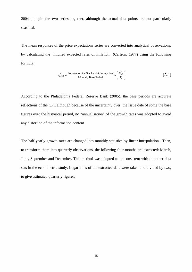
The mean responses of the price expectations series are converted into analytical observations,
by calculating the “implied expected rates of inflation” (Carlson, 1977) using the following
formula:
.PeriodBaseMonthly
dateSurveyatlevelSixtheofForecast 11, ⎟
⎟⎠
⎞⎜⎜⎝
⎛== +
+t
EtA
tt PPπ [A.1]
According to the Philadelphia Federal Reserve Bank (2005), the base periods are accurate
reflections of the CPI, although because of the uncertainty over the issue date of some the base
figures over the historical period, no “annualisation“ of the growth rates was adopted to avoid
any distortion of the information content.
The half-yearly growth rates are changed into monthly statistics by linear interpolation. Then,
to transform them into quarterly observations, the following four months are extracted: March,
June, September and December. This method was adopted to be consistent with the other data
sets in the econometric study. Logarithms of the extracted data were taken and divided by two,
to give estimated quarterly figures.
26
References
Blaug, M. (1997) Economic Theory in Retrospect, Fifth Edition, Cambridge University Press,
Cambridge.
Bywaters, D.S. and Thomas, D.G. (2008) Output Expectations and Forecasting of U.K.
Manufacturing, Atlantic Economic Journal, April, 36, pp 125-137.
Carlson, J. A. (1977) A Study of Price Forecasts, Annals of Economic and Social
Measurements, 6, Winter, pp 27-56.
Cronshore, D. (1997) The Livingston Survey: Still Useful After All These Years, Federal Bank
of Philadelphia, Business Review, March/ April, pp 1-12
De Grauwe, P. And Polan, M. (2005) Is Inflation Always and Everywhere A Monetary
Phenomenon? , Scandinavian Journal of Economics, 107(2), pp 239-259.
Enders, W. (2004) Applied Econometric Time Series, Second Edition, Wiley, Hoboken.
Granger, C. And Lee, T-H (1990) Multicointegration, Advances in Econometrics 8, pp 77-84.
Hendry, D.F. (1983) Econometric Modelling: Consumption in retrospect, Scottish Journal of
Political Economy, 30, pp 193-220.
27
Hendry, D.F. (1987) Economic methodology: a personal perspective, In Advances in
Econometrics: 5th World Congress, Vol.2, (Bewley, T.F., ed.), pp 236 261, Cambridge
University Press, Cambridge.
Hicks, J.R. (1968) Value and Capital, Second Edition, Clarendon Press, Oxford.
Johansen, S. (1988) Statistical Analysis of Cointegration Vectors, Journal of Economic
Dynamics and Control, 12, June-September, pp 231-254.
Keynes, J.M. (1936) The General Theory of Employment, Interest and Money, Macmillan
Cambridge University Press, Cambridge.
Livingston Survey Documentation (2005), Federal Reserve Bank of Philadelphia, December.
Maddison, A. (2003) The World Economy: Historical Statistics, OECD. Publications, Paris.
Morana, C. And Bagliano, F.C. (2007) Inflation and Monetary Dynamics in the U.S.A.: a
quantity-theory approach, Applied Economics, 39, pp 229-244.
Pesando, J.E. (1975) A Note on the Rationality of the Livingston Price Expectations, Journal of
Political Economy, 83, August, pp 849-58.
Popper, K. (1970) The Poverty of Historicism, Routledge and kegan Paul, London.
Stock, J. And Watson, M. (1988) Testing for Common Trends, Journal of the American
Statistical Association, 83, December, pp 1097-1107.
28
Thomas, D.G. (1995) Output Expectations within manufacturing Industry, Applied Economics,
27, pp 403-08.
Wicksell, K. (1936) Interest and Prices, Macmillan and Co., Ltd, St. Martin’s Street, London.
Woodford, M. (2003) Interest and Prices: Foundations of a Theory of Monetary Policy,
Princeton University Press, Princeton.


