1

Estudios Económicos Volume 14, Number 1, Enero-Junio 1999, Pages 33-52

Inflationary Pressure Determinants in Mexico*

Thomas M. Fullerton, Jr. Fulbright Mexico Scholar

Department of Economics & Finance University of Texas at El Paso

El Paso, TX 79968-0543 Telephone: (915) 747-7747 Facsimile: (915) 747-6282

Email: tomf@utep.edu

Cuauhtémoc Calderón Villarreal Departamento de Economía

Universidad Autónoma de Ciudad Juárez Ciudad Juárez, Chihuahua

México Telephone: (16) 16-69-60 Facsimile: (16) 13-83-79 Email: ccaldero@uacj.mx

Abstract An ongoing difficult policy issue confronting monetary authorities in many developing economies is the management of a stable price environment. Unstable prices create uncertainty, lower investment, and raise costs of doing business, thus lowering rates of growth. As a result, there exists a widespread need for understanding inflationary dynamics in any country of interest. This paper develops a standard monetary inflation model and augments it to include import and labor cost of production factors in a theoretically plausible manner. Implications for implementing an empirical version of the model are also discussed.

2

Inflationary Pressure Determinants in Mexico Introduction Virtually every Latin American economy must deal with the impacts of inflation in one manner or another. In general, inducing a stable price environment is regarded as a key step to improving economic welfare by enabling any given economy to operate more efficiently. This argument applies equally well to advanced economies such as the United States (Motley, 1998) as well as developing nations (Zind, 1993). This argument bears particular relevance in Mexico due to the inflationary aftershock which followed the tequila effect December 1994 peso devaluation. An important plank within the Zedillo government policy package is attaining price stability. A critical step in implementing such a policy effort is gaining an accurate understanding of the price dynamics at play in the Mexican economy. This paper presents a theoretical modeling framework for the purpose of analyzing the sources of developing country inflationary pressures. A standard monetary model is adapted to incorporate two important factor costs of production, labor and imported inputs, in a mathematically consistent manner. Several empirical versions of the resulting model are estimated in order to examine the historical behavior of Mexican consumer price movements. Subsequent material in the study offers a review of the literature, theoretical model, and empirical results. Suggestions for future research are summarized in the conclusion. Literature Review The seminal research on inflationary dynamics in developing countries was conducted on Chilean data by Harberger (1963). That early paper interestingly points out that directly analyzing data in level form could result in spurious correlations in equations estimated for highly inflationary economies. To circumvent this problem, percentage rates of change are utilized in a linear regression framework based on the quantity theory of money. What became known as the “Harberger” framework incorporates real income, current and lagged values of the money supply, and the opportunity cost of holding cash balances. The success of this initial effort conducted on Chilean data spurred a series of replicated studies for other developing countries (for example, see Vogel, 1974). Results generally confirm the overall usefulness of the Harberger model. Following numerous applied econometric studies utilizing this approach, it became apparent that exclusive reliance on domestic variables alone often provides unsatisfactory results. Bomberger and Makinen (1979) provide a thorough examination of the Harberger model using quarterly data for Korea, Taiwan, and Vietnam. Rather than extend the model in a new direction, extensive testing is conducted in order to establish whether a suitable characterization of inflation is provided. Encouragingly, the parameter estimates do not appear sensitive to the time period selected. However, the elasticities with respect to money and real income are not always unitary as hypothesized. Also, the coefficient signs for the cost of holding money variables are sometimes negative.

3

Hanson (1985) extends the Harberger framework in a systematic fashion to incorporate an important missing component, import costs. An implicit cost function is utilized to derive an aggregate supply curve which includes local prices of imported inputs. When the underlying production function is homogeneous of degree one, inflation becomes a weighted sum of money supply changes and import prices. This is important because it implies that the elasticity of inflation with respect to money growth is less than one. Empirical results in the Hanson article strongly support the inclusion of import prices in models of inflation. Subsequent research has provided additional evidence in favor of the augmented Harberger-Hanson approach wherein the effect of import prices on inflation is considered. Koch, Rosensweig, and Witt (1988) and Fullerton, Hirth, and Smith (1991) both report positive linkages between the trade-weighted exchange value of the dollar and consumer prices in the United States. These empirical studies indicate a unidirectional channel of influence from the exchange rate to domestic prices exists in the United States economy. As will be discussed below, causality direction has important implications for both model form and estimation technique. Developing country studies have also confirmed the usefulness of an augmented modeling treatment of inflationary dynamics. Sheehey (1976) reports some of the early econometric work along these lines. Sheehey (1980) reaches additional conclusions on the basis of empirical tests that indicate that accurate assessment of austerity policy efforts will likely require explanatory variables representing cost push factors. More recently, Brajer (1992) provides evidence that the latter category of models may offer better specifications than those which rely solely on domestic economic factors. Similarly, Fullerton (1993a,b) successfully imbeds a variant of this approach in large-scale macroeconometric forecasting models for Colombia and Ecuador using annual data. There have also been a small number of dynamic models estimated on the basis of monthly data for developing economies. Fullerton (1993c) empirically examines Colombian anti-inflationary efforts utilizing monthly data with an autoregressive-moving average (ARMA) transfer function. Separately, Fullerton (1995) develops an econometric model, based in large part on the augmented Harberger-Hanson framework, to examine price stabilization efforts in Ecuador. The estimated models for both economies are found to generate realistic simulation scenarios for policy analysis. Results reported in both articles also support the hypothesis of inflation rate inelasticity with respect to money supply growth. Theoretical Model Harberger's (1963) model is based on the traditional quantity theory of money equation: 1. MV = PQ, where M represents some measure of the money stock, V is the velocity of circulation, P is the price level, and Q is real output. The realism of the model is enhanced by allowing velocity to vary

4

instead of arbitrarily forcing it to be constant. Velocity is assumed to be a predictable function of other macroeconomic variables that reflect the cost of holding cash balances. To utilize percentage changes, the variables can be transformed by natural logarithms and first differenced. Introduction of a time subscript, and rearrangement of the terms, yields the basic Harberger equation: 2. DPt = DMt - DQt + D(It-1), where the last term results from substituting for velocity and D represents a difference or backshift lag operator. Harberger substitutes for velocity, using the lagged change in the inflation rate to proxy for the implicit cost of holding money. This approach is useful when modeling inflation in countries where government banking system regulations have occasionally caused savings and loan rates to become fixed in nominal terms and temporarily negative in real terms. Unadjusted interest rates from these periods would obviously not provide accurate estimates for the cost of holding cash. In economies where financial markets have been allowed to operate more flexibly, and where appropriate data have been recorded, an interest rate series may also be used to define the last explanatory variable in Equation 2. Because Mexico has allowed fairly substantial interest rate flexibility since 1982, Equation 2 contains an interest rate as the last right-hand side variable. Equation 2 implies that inflation will vary positively with the money supply and inversely with respect to real output. A statistically significant intercept term will enter the estimated equation if there is a trend in the velocity of circulation. If only contemporaneous lags of M and Q enter in the equation, the parameters for both variables are hypothesized to be unitary. This can be tested empirically with the following specification: 3. DPt = a0 + a1DMt - a2DQt + a3D(It-1) + u3, where a1 and a3 are hypothesized to be positive, and the absolute values of a1 and a2 should both be statistically indistinguishable from one. The last argument in the expression represents the disturbance term. Hanson (1985) proposes a cost function which is homogeneous of degree one to allow for the incorporation of factor prices in the modeling framework. Derived output supply functions from this framework will be homogeneous of degree zero in input and output prices. Equation 4 expresses this relationship using logarithmic first differences: 4. DQt = b0 + b1DPt - b2DPIt + u4, where PI represents imported input prices. When the relative prices of imported inputs increase, output is assumed to decline. The standard homogeneity assumptions for production and derived supply relations imply that b1 - b2 = 0.

5

The vector of input prices utilized in the derivation of Equation 4 can be extended to include factor prices beyond those represented by imported materials, equipment, and services. Perhaps the most obvious candidate to further improve the relevance of the framework is labor costs (Fullerton, 1999). Doing so yields the following theoretical expression: 5. DQt = b0 + b1DPt - b2DPIt - b3DWt + u5, where W represents wage and labor costs. In this case, the standard microeconomic assumptions for production and derived supply functions imply that b1 - b2 - b3 = 0. Equation 5 can be substituted into Equation 3 to eliminate the output term from the expression to be estimated. This step is exceedingly useful for avoiding interpolation bias in empirical studies of monthly inflation for countries where national income and product accounts are published at quarterly and/or annual frequencies (for a discussion of interpolation bias, see Bomberger and Makinen, 1979). The resulting equation can be written as follows: 6. (1 + a2b1)DPt = a0 - a2b0 + a1DMt + a2b2DPIt + a2b3DWt + a3D(It-1) + u6. Equation 6 can be further simplified prior to estimation. Dividing through by the left-hand side constant term and rearranging terms such that the price series remains as the dependent variable generates the following relation: 7. DPt = c0 + c1DMt + c2DPIt + c3DWt + c4D(It-1) + u7, which also has testable properties. Note that the coefficient on the monetary variable, c1, is hypothesized to be significantly less than one. With the possible exception of the intercept, all of the regression parameters in Equation 7 are expected to be positive. In earlier studies for other countries such as Ecuador, Nigeria, and the United States (Fullerton, 1995; Fullerton and Ikhide, 1998; Fullerton, Hirth, and Smith, 1991), it has been necessary to substitute the import price deflator with an exchange rate series due to data constraints. That substitution may not be necessary in the case of modeling annual consumer price movements in Mexico since the central bank has developed an import price deflator with historical observations that date back more than two decades. As indicated in the literature review, this general approach has provided a useful framework for analyzing annual inflation rates. But because the implied lag structure is fairly short, it may require additional modification prior to estimation. This possibility does not reflect any deficiencies in the theoretical model as such, but arises due to the fact that dynamic modeling in economics does not offer clear guidelines with respect to lag-length specification. As a result, if the inflationary impact of a change in the money supply is felt over the course of more than one calendar year, the implied lag structure for a model estimated with monthly data could potentially exceed that which is shown above. Equation 8 takes into account this empirical issue which has confronted and confounded researchers for many years (see Laidler, 1993):

6

8. DPt = c0 + Sum(c1i)DMt-i + Sum(c2jDPIt-j) + Sum(c3k)DWt-k + Sum(c4m)D(It-1-m) + u8, where i,j,k,m = 0,1,2,…, respectively. Implications for Estimation The above model provides an attractive starting point for examining inflationary trends in an economy. It is not, however, without potential problems for analyzing price movements. The principal concern with this theoretical construct arises from the fact that Equation 8 treats all of the regressors as exogenous or pre-determined. In doing so, it does not allow for the possibility of statistical feedback or endogeneity between the left-hand and right-hand side variables. If a central bank yields to political pressures and engages in accommodative monetary policy in the face of inflation shocks, this assumption would be violated. Research conducted using both monthly and quarterly data for Colombia indicates that the causality paths are unidirectional as implied by Equation 8 (see Fullerton, 1993c, and Leiderman, 1984). This assumption may not always be satisfied. Domestic prices, monetary aggregates, and import prices are modeled simultaneously in a large-scale Colombian macroeconometric model estimated using annual data by Fullerton (1993a). It would not be surprising if the feedback relations encountered in the latter paper also emerge in higher-frequency data samples, especially in cases where monetary authorities are forced to yield to political pressures. This likelihood is even greater in economies where wages and prices are linked via formal indexing rules and other types of cost-of-living escalator clauses in labor agreements (Dornbusch and Fischer, 1993). A second possible concern arises from utilizing first differenced, log-transformed time series data in the equation to be estimated. If the resulting series are stationary, the equation can be estimated without risk of obtaining spurious correlations in the results. As shown in many studies of hyperinflationary economies, however, higher order differencing may be required to induce stationarity during periods in which prices increase rapidly (see Engsted, 1993). Because Mexico has never experienced any hyperinflationary episodes, regular first differencing should adequately remove nonstationary trends in the first moments of any variables selected for analysis. It is still important, however, to formally test the latter assumption when empirical versions of Equation 8 are estimated. In order to examine whether the working series included in Equation 8 are stationary, a variety of unit root tests may be utilized. For some developing economies where data limitations are severe, applying unit root tests to relatively short time spans may be risky. The latter consideration is due to the fact that these tests typically have low power unless long-run data sets are employed (Hakkio and Rush, 1991). Time series data for consumer prices and exchange rates generally date back to 1957 and do not pose any problems. For other variables such as money supply aggregates, wages, and interest rates, there may be little that can be done to circumvent this

7

potential problem. In such cases, chi-square tests calculated for autocorrelation functions (Greene, 1993) may provide corroborative evidence to support the results obtained from the unit root tests. As specified above, the model is explicitly built around a set of unidirectional causality relations from movements in the regressors to consumer prices. To examine whether the absence of simultaneity in the model is plausible, Granger causality tests may be calculated for the stationary components of the series of interest. If the resulting F-tests fail to reject the feedback hypothesis, then the reduced form model appearing in Equation 8 is inadequate. Potential alternative candidate approaches include structural model systems of equations (Beltrán del Río, 1991, and Fullerton and Araki, 1996) and vector autoregression equation systems (Arellano and Gonzalez, 1993). The model developed above accounts for more potential sources of inflation than do previous versions of the Harberger-Hanson theoretical framework. Its scope still may not be wideranging enough to explain all systematic variations in aggregate price levels for particular economies. If this is the case, the shortcoming will be manifested in the form of serially correlated residuals. If it is not possible to identify and extend the model to resolve the nonrandom component of the residuals, then the autocorrelation should be corrected in order to minimize the possibility of spurious estimation results (Hamilton, 1994). Pagan’s (1974) nonlinear ARMAX procedure offers an attractive option because of its capacity to handle autoregressive, moving average, and mixed error generating processes. The lag structure in Equation 8 is arbitrary by design. In estimation, however, specific lag lengths must be selected. Ultimately, this question is an empirical one. Experimentation with the lag structure generally cannot be avoided in any modeling process involving dynamic specifications. Several decision rules are available. Examples include likelihood ratio tests, Akaike, and Schwarz criteria. Previous Latin American research cited above, however, indicates that the usage of annual data within the overall framework developed herein is not likely to require long lag lengths. Cognizant of the exploratory characteristics of the model developed herein, a variety of simulation exercises will be mandatory in evaluating empirical versions of Equation 8. The goal of the simulation tests is to provide insights with respect to the policy analytic and extrapolation accuracy validity of the underlying theoretical model. Usage of out-of-sample data not employed in parameter estimation provides the only means by which the simulation experiments can satisfy the Klein (1984) and Christ (1993) criteria for forecast and model evaluation. Although model development and hypothesis testing are the primary goals of the research at hand, a sample set of monetary policy simulation exercises are also reported below. Empirical Results Equation estimation is conducted for two sample periods, 1970-1997 and 1975-1997. The initial period starting point is determined by data availability at the Banco de Mexico internet web site (www.banxico.org.mx). At present, that web site serves as a tremendous tool to researchers

8

located outside Mexico City. Data coverage at the web site is expanding rapidly and offers a timely means for acquiring macroeconomic and balance of payments data. The second sample period starting point is selected to correspond with the period during which nominal exchange rates have changed with a higher degree of frequency than was observed between 1954 and 1976. The split sample approach is useful because it provides a means for examining the possibility of parameter heterogeneity due to policy innovations observed in recent decades in this economy (Fullerton and Sprinkle, 1997). As noted above, Mexico has never experienced hyperinflation (price changes of 50 percent per month or higher). Given this, it not surprising that first moment stationarity is obtained after first-order differencing is performed on logarithmic transformations of the original series. As underscored by the unit root test results shown in Table 1, this allows a straightforward application of the theoretical framework developed above. Granger causality F-tests reported in Table 2 confirm the absence of feedback effects across both sides of the equation, implying that parameter estimation will not be required to handle simultaneity. The latter results are obtained for two- and three-year lags of the dependent and independent variables appearing in Equation 8. That the results are in contrast to those earlier reported by Leiderman (1984) for Mexico possibly reflects the substantial turnabouts witnessed in Mexican monetary policy since 1988. Parameter estimation results for equation 8 are reported in Appendix A. Fairly strong evidence in favor of the theoretical model is made apparent by the high degree of coefficient stability across sample periods. Also remarkable is the absence of serial correlation problems, also underscored by relative coefficient stability between the corrected and non-corrected estimates of the equations. Of primary importance is the fact that the results consistently point to the same variables as the sources of inflationary pressures in Mexico. In Appendix A, Equation A1 is estimated over the entire sample period, 1971-1997. Although the F-statistic is highly significant, three of the regression coefficients are statistically insignificant as a consequence of multicollinearity. Of even greater concern is the fact that the estimated parameter for the stationary component of the import price deflator is negative instead of positive as hypothesized. The other parameters have the theorized signs and are in line with results and inferences reported elsewhere (Caire and Calderón, 1996; Jarque and Tellez; 1993; Pérez-López, 1996). Contemporaneous lags for money, import prices, and wages, plus an additional lag on the interest rate are sufficient to satisfactorily explain changes in the dependent variable. The latter is confirmed by the Durbin-Watson statistic reported in the appendix. The six-lag correlogram chi-square analysis reported in Appendix A does not reveal evidence of higher order serial correlation or indicate that higher order lags of the regressors are required to adequately account for inflationary trends in Mexico. The Akaike and Schwarz criteria estimates also appear in the appendix output. Given the fact that Mexican monetary policy from 1954 through 1975 established a fixed nominal exchange rate with respect to the dollar, it is natural to question whether the empirical estimates reported for the full sample period are valid. To address the issue of potential parameter

9

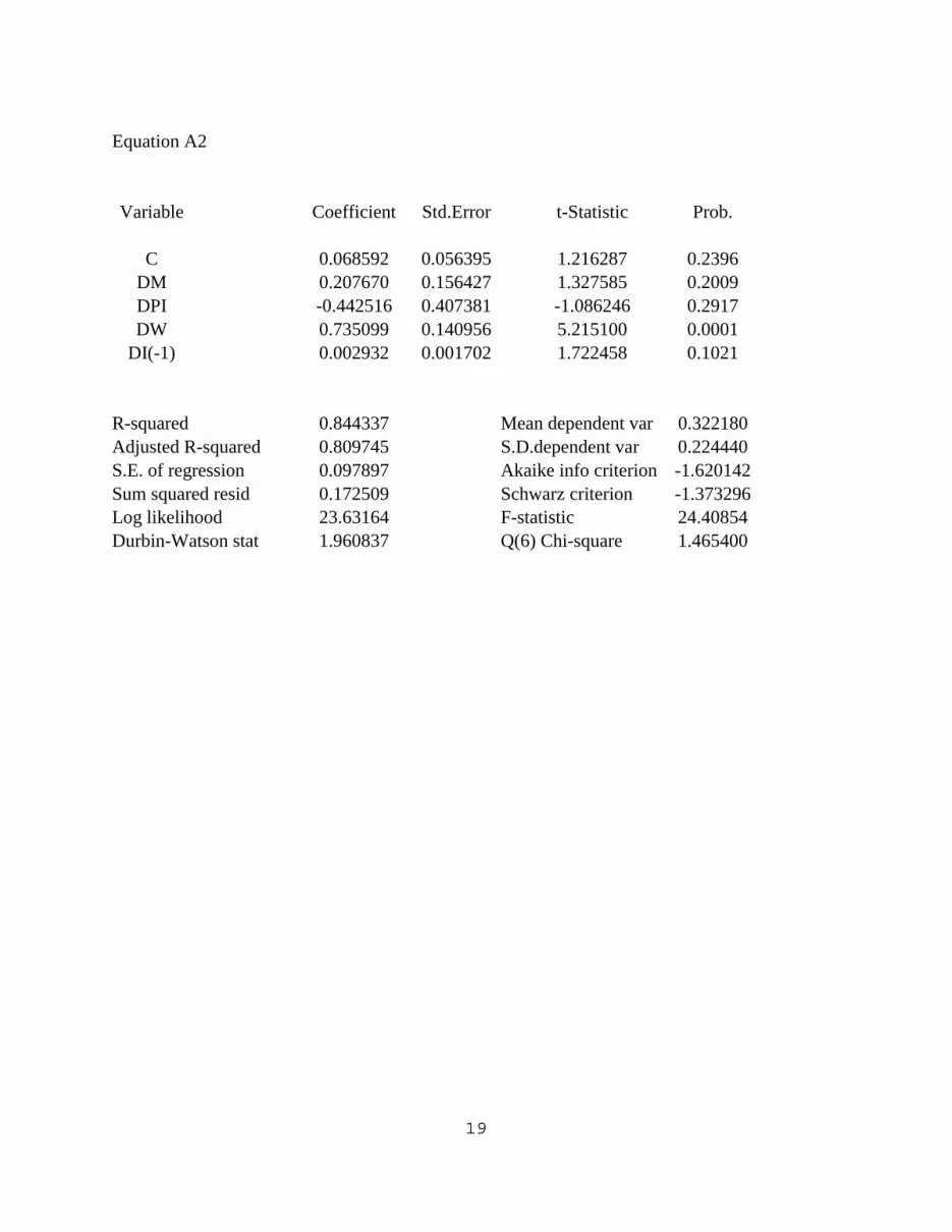
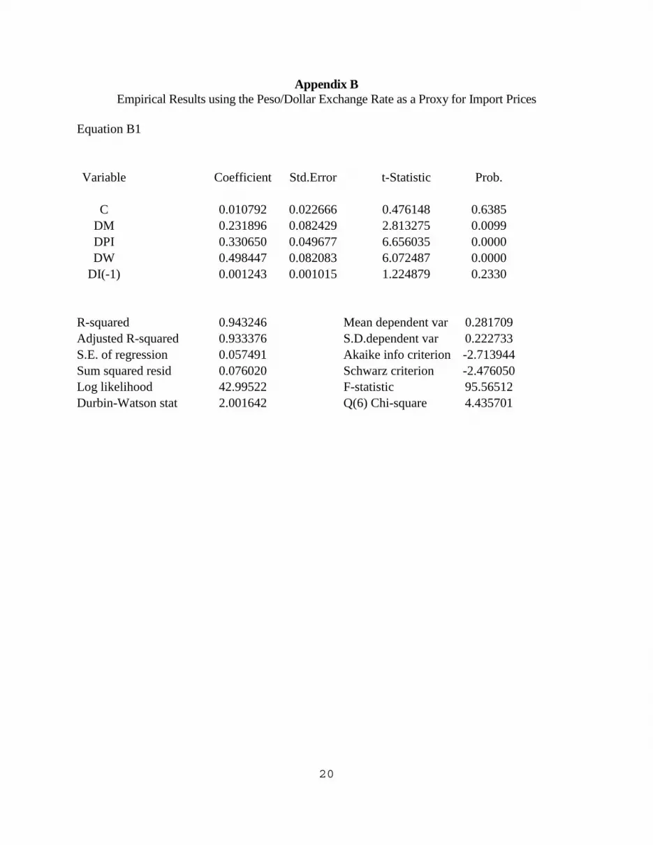
heterogeneity, the sample is shortened to cover the twenty three years from 1975 through 1997. This is the only period in Mexican economic history during which nominal exchange rates have been managed with a high degree of flexibility by the central bank. Similar to Equation A1, the import price deflator coefficient in Equation A2 carries a negative algebraic sign that runs counter to the underlying theoretical model. Multicollinearity remains present in the right-hand-side variable matrix. While the magnitudes of calculated parameter estimates for the original variables included in the model remain virtually identical to those of Equation A1, Chow tests for parameter heterogeneity are not conducted due to the conterintuitive sign associated with the import price deflator coefficient. There is no plausible reason for import price inflation to lead to domestic price deflation in an open economy such as that of Mexico. Because of the unexpected outcomes with respect to the signs attached to the import price deflator, additional models are estimated using a specification that utilizes the peso/dollar nominal exchange rate as a proxy for international price pressures. Equation B1 is estimated for the 1970-1997 time period. All of the parameter estimates are below unity as hypothesized by the underlying theoretical model. Further, all of the coefficients are algebraically greater than zero in line with a priori expectations. Generally good statistical traits are also exhibited by Equation B1. Regression coefficients for the monetary, exchange rate, and wage variables all have t-statistics associated with them that exceed the 5-percent significance threshold. The interest rate variable parameter, however, is not significant. Similar to Equation A1, serial correlation is not encountered in the residuals. The log likelihood coefficient for B1 easily exceeds that of A1, implying econometric superiority on the part of the specification utilizing the exchange rate. The 6-lag chi-square correlogram reported in Appendix B does not uncover any specification problems due to omitted regressor lags. Equation B2 is estimated for the 1975-1997 time frame to allow for potential parameter instability resulting from the aforementioned shift in currency valuation regimes. Once again, the parameters all carry the hypothesized algebraic signs and magnitudes. As with the full sample estimate, the model coefficient associated with the implicit cost of holding idle cash balances does no meet the 5-percent significance criterion. The log likelihood coefficient exceeds that associated with the alternative import deflator version of the equation. Random residual distribution is confirmed by the Durbin-Watson and correlogram data for B2. The Chow F-test for coefficient heterogeneity is 1.726 and statistically insignificant at the 5-percent level for 5 and 41 degrees of freedom. Given this result, complete sample information is utilized in the simulation experiment conducted below. An important question to consider is whether these in-sample estimation results can be replicated under out-of-sample simulation conditions. To at least partially examine this issue, Equation B1 is re-estimated for the 1970-1992 sample period. The resulting equation is then simulated for the 5-year 1993-1997 period using actual historical data to construct an ex-post forecast simulation. As shown in Appendix B, Equation B3 exhibits generally good econometric traits and does not fail to explain any systematic movements in the consumer price index.

10

Predicted annual average inflation rates using Equation B3 are compared with actual average price index increases in Table 3. In three of the years appearing in the tabulated results, the model over-shoots the observed inflation rate, while in the remaining two under-shooting occurs. During the devaluation and recession years of 1995 and 1996, the model simulations err by approximately 20 percentage points from the average rates posted. The 24-month average rate is almost identical to the historical value observed during that period of temporary turbulence and adjustment in the macroeconomy. The estimation and simulation results appearing in the appendices and Tables 1 through 3 confirm the overall usefulness of the underlying theoretical model. Parameter estimates for the money, exchange rate, and cost of holding cash balance proxy variables are significant and robust with respect to sample period changes. Ex-post forecast results envelope the historical sample observations without any evidence of simulation bias emerging. Because the exchange rate equations out perform the import price deflator equations and because the interest rate parameters do not reach 5-percent significance threshold, further empirical testing is necessary. Given the wide ranging cyclical and policy regime conditions observed during the sample estimation periods, the overall usefulness of this general modeling approach is fairly well underscored and future applications appear likely to meet with success. Conclusion An inflationary model is developed above that includes both monetary and factor cost effects in a theoretically plausible manner. Specification and estimation of the model and its parameters are relatively easy to accomplish. Because the model does not pose stringent data requirements, it is likely to be applicable to most developing economies where inflation remains a problem. Given its dynamic specification, the model may be useful in cases where monetary officials continue to grapple with short-term price stabilization goals and high frequency data are utilized. Empirical results indicate that the factors that have contributed most significantly to consumer price pressures in Mexico have been liquidity growth, nominal currency depreciation, and labor costs. Evidence regarding the role of interest rate movements is mixed, but carries the expected algebraic effect in all of the estimation results. The overall specification of the model is relatively robust. Without exception, the diagnostic tests indicate that the model successfully explains all systematic movement in the dependent variable. Coefficients for the statistically significant variables are stable across sample periods and estimation procedures. Because of the latter, this basic modeling approach appears to offer promise as a viable platform for both policy analytic questions as well as business forecasting exercises. Over the sample period in question, endogeneity between inflation, money, wages, the peso/dollar exchange rate, and interest rates does not appear to pose any constraints on choice of estimator or model structure. Even though it is not required for parameter estimation consistency, it might be of interest to imbed the framework developed above into a large scale system of equations.

11

Doing so could potentially enrich subsequent policy and business outlook simulation analyses. The results shown in Table 3 suggest that the model developed herein performs fairly reliably in this context. Ultimately, empirical research utilizing this general modeling approach may help to unravel some of the questions that frequently arise with respect to price trends in Mexico and other developing economies.

12

References Rogelio Arellano Cadena and Eduardo Gonzalez Casteñon, 1993, “Dinámica de la Inflación,” Estudios Económicos 8, 249-261. Banco de México, Worldwide Web Internet Site, www.banxico.org.mx. William A. Bomberger and Gail E. Makinen, 1979, “Some Further Tests of the Harberger Inflation Model using Quarterly Data,” Economic Development and Cultural Change 27, 629-644. Abel Beltran del Río, 1991, “Macroeconometric Model Building in Latin American Countries, 1965-1985,” Chapter 12 in A History of Macroeconometric Model Building, Edited by Ronald G. Bodkin, Lawrence R. Klein, and Kantah Marwah, Brookfield, VT: Edward Elgar Publishing. Victor Brajer, 1992, “Empirical Inflation Models in Developing Countries,” Journal of Development Studies 28, 717-729. Gilles Caire and Cuauhtemoc Calderón, 1996, “Crise Mexicaine de 1995: Les Lecons d’une Expérience Hétérodoxe de Stabilisation Macroéconomique,” Economie Appliquée 49, 79-105. Carl Christ, 1993, “Assessing Applied Econometric Results,” Federal Reserve Bank of St. Louis Review 75 (March/April), 71-94. Rudiger Dornbusch and Stanley Fischer, 1993, “Moderate Inflation,” World Bank Economic Review 7, 1-44. Tom Engsted, 1993, “Cointegration and Cagan's Model of Hyperinflation under Rational Expectations,” Journal of Money, Credit and Banking 25, 350-360. Thomas M. Fullerton, Jr., 1993a, “Un Modelo Macroeconométrico para Pronosticar la Economía Colombiana,” Ensayos Sobre Política Económica 24, 101-136. Thomas M. Fullerton, Jr., 1993b, “Un Modelo Macroeconométrico para Pronosticar la Economía Ecuatoriana,” Cuestiones Económicas 20, 59-100. Thomas M. Fullerton, Jr., 1993c, “Inflationary Trends in Colombia,” Journal of Policy Modeling 15, 463-468. Thomas M. Fullerton, Jr., 1995, “Short-Run Price Movements in Ecuador,” Proceedings of the American Statistical Association, Business and Economic Statistics Section, 280-285.

13

Thomas M. Fullerton, Jr., 1999, “A Theoretical Model of Developing Country Inflationary Dynamics,” Southwestern Journal of Economics 2, 176-191. Thomas M. Fullerton, Jr. and Eiichi Araki, 1996, “New Directions in Latin American Macroeconometrics,” Economic and Business Review 38, 49-73. Thomas M. Fullerton, Jr., Richard Hirth, and Mark Smith, 1991, “Inflationary Dynamics and the Angell-Johnson Proposals,” Atlantic Economic Journal 19, 1-14. Thomas M. Fullerton, Jr. and Sylvanus I. Ikhide, 1998, “An Econometric Analysis of the Nigerian Consumer Price Index,” Journal of Economics 24, 1-15. Thomas M. Fullerton, Jr., and Richard L. Sprinkle, 1997, “Reforms Promote Progress throughout Latin America,” Forum for Applied Research and Public Policy 12 (Winter), 86-89. William H. Greene, 1993, Econometric Analysis, New York, NY: Macmillan Publishing. Craig Hakkio and Mark Rush, 1991, “Cointegration: How Short is the Long-Run?,” Journal of International Money and Finance 10, 571-581. James D. Hamilton, 1994, Time Series Analysis, Princeton, NJ: Princeton University Press. James A. Hanson, 1985, “Inflation and Imported Input Prices in some Inflationary Latin American Economies,” Journal of Development Economics 18, 395-410. Arnold Harberger, 1963, “The Dynamics of Inflation in Chile,” Chapter 2 in Measurement in Economics: Studies in Mathematical Economics and Econometrics in Memory of Yehuda Grunfeld, edited by Carl F. Christ, Stanford, CA: Stanford University Press. Carlos Jarque and Luis Tellez, 1993, El Combate a la Inflación, Mexico, DF: Editorial Grijalbo. Linda Kamas, 1995, “Monetary Policy and Inflation under the Crawling Peg: Some Evidence from VARs for Colombia,” Journal of Development Economics 46, 145-161. Lawrence R. Klein, 1984, “The Importance of the Forecast,” Journal of Forecasting 3, 1-9. Paul D. Koch, Jeffrey A. Rosensweig, and Joseph A. Witt, 1988, “The Dynamic Relationship between the Dollar and U.S. Prices,” Journal of International Money and Finance 7, 181-204. David Laidler, 1993, “Commentary on Assessing Applied Econometric Results,” Federal Reserve Bank of St. Louis Review 75 (March/April), 101-102.

14

Leonardo Leiderman, 1984, “On the Monetary-Macro Dynamics of Colombia and Mexico,” Journal of Development Economics 14, 183-201. Brian Motley, 1998, “Growth and Inflation,” Federal Reserve Bank of San Francisco Economic Review, Number 1, 15-28. Adrian Pagan, 1974, “A Generalised Approach to the Treatment of Autocorrelation,” Australian Economic Papers 13, 260-280. Alejandro Pérez-López Elguézabal, 1996, “Un Estudio Econométrico sobre la Inflación en México,” Documento de Investigación 9604, Banco de México. Edmund J. Sheehey, 1976, “The Dynamics of Inflation in Latin America: Comment,” American Economic Review 66, 692-694. Edmund J. Sheehey, 1980, “Money, Income, and Prices in Latin America,” Journal of Development Economics 7, 345-357. Richard C. Vogel, 1974, “The Dynamics of Inflation in Latin America, 1950-1969,” American Economic Review 64, 102-114. Richard G. Zind, 1993, “On Inflation and Growth in the LDCs,” Economic Studies Quarterly 44, 108-116.

15

Table 1 Augmented Dickey Fuller Unit Root Stationarity Tests

Variable ADF Test Statistic 1% MacKinnon Critical Value DP -5.833 -2.632 DM -5.149 -2.632 DPI -4.503 -2.665 DW -5.392 -2.632 DI -5.747 -2.656

16

Table 2 Pairwise Granger Causality Tests

Variable Direction F-Statistic Probability DM => DP 3.874 0.032 DP => DM 2.301 0.118 DPI => DP 1.146 0.338 DP => DPI 0.690 0.513 DW => DP 3.316 0.071 DP => DW 22.827 0.001 DI => DP 12.974 0.001 DP => DI 0.519 0.512

17

Table 3 Consumer Price Index Ex-Post Forecast Results

Year Predicted CPI Percentage Change Actual CPI Percentage Change 1993 8.3 9.8 1994 10.9 7.0 1995 14.9 36.0 1996 52.5 33.4 1997 24.5 20.6

18

Appendix A Empirical Results using Banco de México’s Import Price Deflator Series

Equation A1

Variable Coefficient Std.Error t-Statistic Prob.

C 0.043743 0.049014 0.892463 0.3818 DM 0.268696 0.147254 1.824704 0.0817 DPI -0.388987 0.383739 -1.013674 0.3218 DW 0.712499 0.130934 5.441657 0.0000

DI(-1) 0.002956 0.001648 1.793974 0.0866

R-squared 0.840742 Mean dependent var 0.290261 Adjusted R-squared 0.811786 S.D.dependent var 0.222242 S.E. of regression 0.096417 Akaike info criterion -1.674699 Sum squared resid 0.204516 Schwarz criterion -1.434729 Log likelihood 27.60843 F-statistic 29.03520 Durbin-Watson stat 2.023158 Q(6) Chi-square 1.587300

19

Equation A2

Variable Coefficient Std.Error t-Statistic Prob.

C 0.068592 0.056395 1.216287 0.2396 DM 0.207670 0.156427 1.327585 0.2009 DPI -0.442516 0.407381 -1.086246 0.2917 DW 0.735099 0.140956 5.215100 0.0001

DI(-1) 0.002932 0.001702 1.722458 0.1021

R-squared 0.844337 Mean dependent var 0.322180 Adjusted R-squared 0.809745 S.D.dependent var 0.224440 S.E. of regression 0.097897 Akaike info criterion -1.620142 Sum squared resid 0.172509 Schwarz criterion -1.373296 Log likelihood 23.63164 F-statistic 24.40854 Durbin-Watson stat 1.960837 Q(6) Chi-square 1.465400

20

Appendix B Empirical Results using the Peso/Dollar Exchange Rate as a Proxy for Import Prices

Equation B1

Variable Coefficient Std.Error t-Statistic Prob.

C 0.010792 0.022666 0.476148 0.6385 DM 0.231896 0.082429 2.813275 0.0099 DPI 0.330650 0.049677 6.656035 0.0000 DW 0.498447 0.082083 6.072487 0.0000

DI(-1) 0.001243 0.001015 1.224879 0.2330

R-squared 0.943246 Mean dependent var 0.281709 Adjusted R-squared 0.933376 S.D.dependent var 0.222733 S.E. of regression 0.057491 Akaike info criterion -2.713944 Sum squared resid 0.076020 Schwarz criterion -2.476050 Log likelihood 42.99522 F-statistic 95.56512 Durbin-Watson stat 2.001642 Q(6) Chi-square 4.435701

21

Equation B2

Variable Coefficient Std.Error t-Statistic Prob.

C 0.020134 0.027484 0.732581 0.4732 DM 0.198040 0.088171 2.246092 0.0375 DPI 0.316275 0.052068 6.074334 0.0000 DW 0.531728 0.088689 5.995394 0.0000

DI(-1) 0.001235 0.001042 1.184288 0.2517

R-squared 0.945615 Mean dependent var 0.322180 Adjusted R-squared 0.933529 S.D.dependent var 0.224440 S.E. of regression 0.057865 Akaike info criterion -2.671746 Sum squared resid 0.060271 Schwarz criterion -2.424900 Log likelihood 35.72508 F-statistic 78.24312 Durbin-Watson stat 1.748572 Q(6) Chi-square 2.382399

22

Equation B3

Variable Coefficient Std.Error t-Statistic Prob.

C -0.014119 0.031048 -0.454736 0.6547 DM 0.325232 0.108323 3.002444 0.0076 DPI 0.263370 0.067282 3.914416 0.0010 DW 0.527308 0.090500 5.826602 0.0000

DI(-1) 0.001403 0.001275 1.099728 0.2859

R-squared 0.948864 Mean dependent var 0.301940 Adjusted R-squared 0.937500 S.D.dependent var 0.237306 S.E. of regression 0.059326 Akaike info criterion -2.621866 Sum squared resid 0.063353 Schwarz criterion -2.375019 Log likelihood 35.15146 F-statistic 83.50012 Durbin-Watson stat 2.044918 Prob.(F-statistic) 1.649402