arX

iv:h

ep-p

h/01

0324

3v2

17

May

200

1

OUTP-00-41P (rev)

Low-scale inflation

Gabriel GermanCentro de Ciencias Fısicas, Universidad Nacional Autonoma de Mexico, Apartado Postal 48-3,

62251 Cuernavaca, Morelos, Mexico

Graham Ross and Subir SarkarTheoretical Physics, University of Oxford, 1 Keble Road, Oxford OX1 3NP, UK

(February 1, 2008)

Abstract

We show that the scale of the inflationary potential may be the electroweak

scale or even lower, while still generating an acceptable spectrum of primordial

density perturbations. Thermal effects readily lead to the initial conditions

necessary for low scale inflation to occur, and even the moduli problem can

be evaded if there is such an inflationary period. We discuss how low scale

inflationary models may arise in supersymmetric theories or in theories with

large new space dimensions.

98.80.Cq, 04.65.+e, 98.65.Dx, 98.70.Vc

Typeset using REVTEX

1

I. INTRODUCTION

Inflation provides an attractive context for discussion of the initial conditions of thehot big bang cosmology, as well as a very plausible mechanism for generation of the scalardensity perturbations which have left their imprint in the anisotropy of the cosmic microwavebackground (CMB) and grown into the observed large-scale structure (LSS) of galaxies [1,2].Field theoretical models of inflation are typically of the ‘slow-roll’ type in which an inflatonfield, φ∗, evolves along a quasi-flat potential to its global minimum. During the roll thevacuum energy is approximately constant and drives an era of exponential growth in thecosmological scale factor a. However such field theory models must explain why the potentialis extremely flat even in the presence of radiative corrections — the “η-problem” — andalso explain why the inflaton field initially lies far from its true minimum.

Quite generally, we may expand the inflaton potential about the value of the field φ∗I just

before the start of the observable inflation era when the scalar density perturbation on thescale of our present Hubble radius 1 was generated, and expand in the field φ ≡ φ∗ − φ∗

I [3].Since the potential must be very flat to drive inflation, φ will necessarily be small while theobservable density perturbations are produced, so the Taylor expansion of the potential willbe dominated by low powers:

V (φ) = V (0) + V ′(0)φ+1

2V ′′(0)φ2 + . . . (1)

The first term V (0) provides the near-constant vacuum energy driving inflation while the φ-dependent terms are ultimately responsible for ending inflation, driving φ large until higher-order terms violate the slow-roll conditions needed for inflation. These terms also determinethe nature of the density perturbations produced, in particular the departure from an exactlyscale-invariant spectrum.

The density perturbation at wavenumber k is given by [2]

δ2H(k) =

1

75π2

V (φ∗ = φ∗H)3

V ′(φ∗ = φ∗H)2M6

, (2)

where φ∗H is the value of the inflaton field when the relevant scale ‘exits the horizon’, i.e.

when k = aH , H ≡ a/a ≃ (V/3M2)1/2, M ≡ MP/√

8π ≃ 2.44× 1018 GeV. The slope of thepotential is given by Eq.(1) as

V ′(φ∗ = φ∗H) = V ′(0) + V ′′(0)φH + . . . ,

where φH ≡ φ∗H−φ∗

I . If the term linear in φ in the potential (1) dominates when the observeddensity perturbations are generated (“linear inflation”), then only the first term above isimportant and the scale of the inflationary potential is required to be near the Planck scale.This can be seen by writing the slope as V ′(0) = cV (0)/M which gives

1Numerically this is H−10 ≃ 3000h−1 Mpc, where h ≡ H0/100 km s−1 Mpc−1 ∼ 0.65 ± 0.15 is

the present Hubble parameter. LSS and CMB observations can measure the density perturbation

down to galactic scales (∼ 1 Mpc), a spatial range corresponding to just 7–8 e-folds of inflation.

2

V 1/4(φ = 0) ≃ (75π2δ2H)1/4c1/2M ∼ 2 × 10−2

√cM, (3)

using the COBE determination of δH ≃ 2×10−5 on the scale of the present Hubble radius [4].We see that the inflationary scale is below the Planck scale (so a field-theoretic descriptionmay be used) but, unless c is unnaturally small, will be not too far below it [1,2].

Examples of models generating linear inflation abound. Consider for example the com-monly used ‘chaotic inflation’2 models in which the inflationary potential is dominated bya monomial, V ∝ φ∗n, and φ∗

I is larger than the Planck scale [5]. The terms in the Taylorexpansion satisfy:

V p+1(φ = 0)φp/V ′(φ = 0) ≃ (φ/φ∗I )p ≪ 1. (4)

Consequently the linear term dominates the φ dependence showing that any such large-fieldinflation model with a monomial potential actually falls into the class of linear inflationmodels defined above. Hence the inflationary scale is not too far below the Planck scale,e.g. for the commonly adopted potential V = 1

2m2φ∗2 one requires m <∼ 10−4M .

There is a circumstance, however, in which it is possible in a natural way to avoidthe conclusion that the inflationary scale is large. This is the case if the linear term isanomalously small. If, as is the usual expectation, the field φ∗ transforms under somesymmetry of the underlying theory, a linear term is forbidden if one expands the potentialabout the symmetric point. In this case the natural expectation is that the next term,namely the quadratic term will dominate. In the large-field inflation model just discussed,this situation does not arise because the initial value of the inflaton field corresponds to a(chaotic) value, and any symmetry under which it is charged is broken. However, as we shalldiscuss, it is possible that the initial conditions are such as to set the inflaton field close tothe origin where the symmetry is unbroken, as in ‘new inflation’ [7]. Provided φ∗

I is alsoclose to the origin, the term linear in φ in the potential (1) will indeed be very small, so thequadratic term may dominate.

It is the purpose of this paper to investigate this possibility (“quadratic inflation”) indetail. Following the same procedure as above we may determine the density perturbationsfor the case of quadratic inflation. Writing V ′′(0) = cV (0)/M2 we now find

δ2H ≃ V (0)3

75π2c2V (0)2φ2HM

2. (5)

Note the appearance of the value, φH, of the (rescaled) inflaton field at the time of productionof the observed density perturbations. Because of this, the scale of the inflationary potentialnow depends on φH:

2The term ‘chaotic’ was in fact originally intended to refer to the initial conditions for the inflaton,

with inflation occuring either at large [5] or small φ [6] field values. However it has come to be

associated exclusively with large-field models with a generic monomial potential, which we discuss

above. To avoid confusion we specifically refer to ‘large-field’ models where relevant. Note that

when inflation occurs at small φ the initial conditions may alternatively be set by thermal effects

[7]. This was originally found to be difficult to implement (hence the proposal of chaotic initial

conditions [5]), but as we shall see these difficulties are circumvented if the inflationary scale is low.

3

V (φ = 0)1/4 ≃ 2 × 10−2√cφ

1/2H M1/2. (6)

Thus if φH/M is small, the scale of inflation will also be small even for natural values ofc ∼ 1. It is clear that quadratic inflation depends sensitively on the terms in the potentialresponsible for ending inflation and determining φH, and that if these terms generate a smallvalue for φH/M then we have a plausible mechanism for low-scale inflation.3

Apart from being of quite general interest quadratic inflation has potential advantagesfor inflation in the case of models with new large dimensions. It has been shown that suchmodels can evade the hierarchy problem associated with the existence of very large massscales because in these models the Planck scale is no longer a fundamental quantity, insteadall fundamental scales are of order the electroweak scale. In these models, however, inflationmust be achieved via a potential which has no large scales and in this context the quadraticinflationary potential is necessary to generate acceptable slow-roll inflation. As we shalldiscuss models with new large dimensions also offer a new way of solving the η-problem.

The alternative explanation of the hierarchy problem is that a new symmetry — super-symmetry — is a good symmetry at low energy scales. As we have remarked earlier [8]supersymmetry provides a very natural source of viable inflatonary potentials. Supersym-metry prevents large radiative corrections to the potential and thus provides a consistentframework to address the η-problem. Furthermore, since thermal effects necessarily breaksupersymmetry, there is also a very natural explanation for why the inflaton field shouldhave its initial high-temperature minimum far from its zero temperature supersymmetricminimum. In quadratic inflation models the scale of inflation can readily be identified withthe scale of supersymmetry breaking.

In this paper we study the construction and implications of quadratic inflationary models,paying particular attention to the mechanisms for solving the η-problem, both in the contextof supersymmetric models and in models with large new dimensions. In Section II we discussthe conditions that must be met by a quadratic inflaton potential in order to generateviable inflation. In Section III we introduce a simple parameterisation of a model capable ofsatisfying these conditions and study in detail in Section IV the characteristics of quadraticinflation. In Section V we discuss how the quadratic inflationary potential can arise insupergravity models and in Section VI we discuss the same question in the context of theorieswith large new dimensions.

II. QUADRATIC INFLATION

Quadratic inflation requires that the inflaton field, φ, rolls from the origin with an in-flationary potential dominated by the quadratic term in a Taylor expansion. In field theorymodels such structure is quite a natural one because scalar fields often carry quantum num-bers under a symmetry such that, in the limit where the symmetry is unbroken, a linear

3A potential with a leading quadratic term was in fact first studied in Ref. [6]. However it was

the steepening of the potential due to this leading term that was assumed there to end inflation

— this implies a relatively high value for φH, hence does not permit a low inflationary scale.

4

term in the potential is forbidden and the quadratic term dominates. Of course it is neces-sary to show that the theory initially starts with the symmetry unbroken, i.e. φ = 0. Weshall demonstrate that this can happen quite naturally through thermal effects because thedimensionless couplings of the theory necessarily respect the symmetry and give a thermalpotential which has a minimum for vanishing φ. It is also necessary that at low tempera-tures the inflaton starts to roll, spontaneously breaking the underlying symmetry. Again,as we shall discuss, this is quite natural as the quadratic mass term often has a negativesign, triggering spontaneous breaking of the symmetry. Provided this mass term is smallit will not affect the high temperature potential significantly but will generate the slow-rollinflation at late times once the temperature drops sufficiently.

Of course this explanation requires that the system initially be in thermal equilibriumand this is not normally the case in slow-roll inflationary models, particularly since theinflaton should be very weakly coupled in order not to spoil the required flatness of itspotential. However quadratic inflation is special in as much as the value of the potentialduring inflation is not strongly constrained by the need to generate the correct magnitude ofdensity perturbations. For the case that the potential energy driving inflation is low, we willshow that the processes leading to thermal equilibrium do have time to establish equilibriumbefore the inflationary era starts.

A further crucial question is why the universe should initially be sufficiently homogeneousfor slow-roll inflation to begin. In chaotic (large-field) inflation models [5], inflation beginswhen the scale of the potential energy is of order the Planck scale and the horizon (the scaleover which the universe must be homogeneous for inflation to start [9]) is also of order thePlanck scale. By contrast in the models discussed here, inflation starts much later whenthe horizon contains many such Planck scale horizons and, in this case, it is difficult tounderstand how the necessary level of homogeneity can be realised. However this argumentis not really a criticism of the possibility that there be a late stage of (quadratic) inflation butrather a statement that this cannot be all there is. Thus we require that there was some otherprocess which ensured the necessary homogeneity at the beginning of quadratic inflation, asin the eternal inflation scenario [10], or perhaps through some quantum cosmological process[11]. Such considerations suggest a situation in which a homogeneous universe emerges atthe Planck era and potential energy is released reheating the universe and, as describedabove, setting the conditions for further periods of inflation to occur. If the late stage ofinflation generates a sufficient number of e-folds of inflation, these earlier eras will not haveobservable consequences for our universe although they will have been crucial in setting thecorrect initial conditions for it to occur.

In a complete field theory description of the fundamental interactions there are usuallymany scalar fields, all candidates for generating a period of inflation. For this reason weconsider quadratic inflation to be a generic feature. Indeed one might expect several infla-tionary periods to be encountered in the evolution of the universe due to several scalar fieldsslow-rolling to their minima. Again only the last such era will be relevant to observation ifit generates a sufficiently large (∼ 50 − 60) number of e-folds of inflation.4

4Multiple short bursts of inflation may also be viable [12], as is indeed suggested by recent CMB

and LSS data [13].

5

A. Slow-roll conditions

Let us turn now to a more detailed discussion of the conditions that a quadratic potentialmust satisfy if it is to generate inflation. Starting from 〈φ〉 ∼ 0 and assuming that thesymmetry properties of the model forbid a linear term, the quadratic term will dominate,giving a new inflation [7] potential of the form5

V (φ) ∼ ∆4 − 1

2m2φφ

2 + . . . , (7)

where the constant vacuum energy ∆4 is now the leading term in the potential.The slow-roll condition is given by [2,14]

ǫ ≡ M2

2

(V ′

V

)2

≪ 1, |η| ≡M2

∣∣∣∣∣V ′′

V

∣∣∣∣∣≪ 1 , (8)

where the potential determines the Hubble parameter during inflation as, Hinf ≡ a/a ≃(V/3M2)1/2. Inflation ends (i.e. a, the acceleration of the cosmological scale factor, changessign from positive to negative) when ǫ and/or |η| becomes of O(1). From Eq.(8) we havenow a constraint on the mass

mφ ≪ Hinf ∼ ∆2/M, (9)

which is much smaller than its natural value — the η-problem. To solve this problem weare driven to consider theories in which mφ is prevented from becoming large.

B. Initial conditions for inflation

What about the initial conditions necessary for inflation to commence? We assume thatsome process at the Planck scale, presumably quantum cosmological in nature [11], createsa homogeneous patch of space-time of sufficient size for our last stage of inflation to occurif the inflaton field satisfies the constraints just discussed.6

During the Planck era the inflaton field has a natural value of O(MP) due to gravitationalinteractions which are strong at this scale. At later times, while φ is still large, its potentialwill be dominated by the highest powers, φp/M ′p−4, in the inflaton potential (where M ′ isa high mass scale in the theory). Such terms will cause the inflaton to flow towards theorigin. However they cannot drive φ to a sufficiently small value for quadratic inflationto occur because they rapidly become negligible as φ becomes small. For this reason it isnecessary to consider whether there exists some other mechanism capable of driving φ small.

5In what follows we will often just use φ to denote its vacuum expectation value (vev).

6In the case of additional dimensions this should presumably occur in the underlying higher

dimensional theory at the higher dimensional Planck scale. The later stage of quadratic inflation

occurs at a scale below the compactification scale when the effective theory is four-dimensional.

6

In particular the thermal potential following from a coupling of the inflaton to other fields χ(e.g. φ2χ2) will contain a term proportional to φ2T 2 which can drive φ to the origin. Thuswe should consider what happens after the Planck era to determine whether the necessarythermal distribution can be created from the potential energy released as the scalar fields,initially at the Planck scale, roll towards their low energy minima.

It is important to note that the thermalisation temperature cannot be close to thePlanck scale, regardless of the amount of energy released. To quantify this let us con-sider the requirements on the inflaton field for it to be localised at the origin through itscouplings to particles in the thermal bath [15]. On dimensional grounds, the 2 → 2 scatter-ing/annihilation cross-sections at energies higher than the masses of the particles involvedare expected to decrease with increasing temperature as ∼ α2/T 2, where α is the coupling.Thus if the scattering/annihilation rate, Γ ∼ n〈σ v〉 is to exceed the Hubble expansion rateHtherm ∼ (g∗T

4/10M2)1/2 in the radiation-dominated plasma, then we have a limit on the

thermalisation temperature Ttherm<∼ α2M/3g

1/2∗ , where g∗ counts the relativistic degrees

of freedom (=915/4 in the minimal supersymmetric standard model (MSSM) at high tem-peratures). Now a coupling g2φ2χ2 of the inflaton to another scalar field χ will generate aconfining potential at high temperatures, V (φ, T ) ∼ g2T 2φ2 i.e. an effective mass for theinflaton of mtherm ∼ gT . This will rapidly drive the inflaton field to the origin in a timeof O(m−1

therm). As the universe cools, the potential energy ∼ ∆4 of the inflaton will beginto dominate over the thermal energy at a temperature Tinf ∼ ∆2/α2M . At this epoch theinflaton field will be localised to a region δφ ∼ Tinf in the neighbourhood of the origin. Thusto provide natural initial conditions for quadratic inflation we require that:

Tinf < Ttherm i.e. ∆ <∼ 10−4M for α ∼ 1/24. (10)

This rough estimate is consistent with the more precise explicit calculation of the qq annihi-lation rate into gluons which finds that equilibrium can only be attained below a temperatureTtherm ∼ 3×1014 GeV [16].7 It is crucial if this mechanism is to work that the field χ shouldhave a mass less than Ttherm otherwise it decouples and does not contribute to the thermalpotential of the inflaton. This is a potential problem because the inflaton vev generatesa mass gφ. However, as we noted above, the term φp/M ′p−4 does drive φ small, givinggφ = gM ′(T/M ′)4/p. Thus a viable model capable of generating the initial conditions forinflation via thermal corrections has to satisfy the rather mild condition

gM ′(T/M ′)4/p < Ttherm. (11)

III. ANALYSIS OF QUADRATIC INFLATIONARY MODELS

In this Section we discuss the implications of quadratic inflation using a general param-eterisation of the inflationary potential. The origin of this potential in specific theories will

7A similar estimate of the thermalisation temperature obtains in a study where cold particles are

released at the Planck scale and allowed to scatter to achieve equilibrium [17].

7

be discussed in subsequent Sections. The potential can be conveniently parameterised asa constant term driving inflation plus a quadratic term with coefficient which may be acombination of a “bare” mass at the Planck scale together with a logarithmically varyingmass term generated by radiative corrections [15]. Thus the full potential has the form

V (φ) = ∆4

1 + b

(|φ|M

)2

+ c ln

(|φ|M

)(|φ|M

)2

. (12)

Note that we have not included a term linear in φ. As we have stressed above such a termcan be forbidden if the theory has a symmetry under which φ transforms non-trivially andwe assume that this is the case. For example φ may be a complex field which transformsunder an Abelian symmetry (or a discrete subgroup) as φ −→ eiαφ. In this case the lowestinvariant we can form is |φ|2 as in Eq.(12) and |φ| is the component of φ that plays the roleof the inflaton. In what follows we shall denote the inflaton simply by φ.

In practice we are mainly interested in Eq.(12) for small φ ∼ φH, the field value whenthe density perturbations now entering our Hubble radius exit the horizon during inflation.In this region we can ignore, to a good approximation, the logarithmic variation of theeffective mass term and write V (φ) ≃ ∆4(1 + bφ2) where b = b + c lnφ2

H and φ, ∆ are nowexpressed in Planck units: φ ≡ φ/M , ∆ ≡ ∆/M . In this case we can solve the evolutionequations analytically. After doing so we shall present numerical solutions to the potentialincluding the logarithmically varying terms and compare with the analytic solution to theapproximate form. Our parameterisation of the scaled potential V (φ) = V (φ)/∆4 is thus:

V (φ) =(1 − κ

∆qφp)2

+ bφ2 + c. (13)

For the case of interest, only the quadratic term is important during inflation. However toallow us to discuss the end of inflation we have included higher-order terms ∝ φp/∆q andabove. These terms are only relevant to the behaviour at the end of inflation; motivationfor this specific form is provided later (Section VC2). We have also included a constant,c to allow the potential to vanish at the end of inflation. Note that a severe fine tuning inthe value of c is needed to cancel the contribution of the other terms at the true minimumof the potential. Since, to date, there is no explanation for the observed smallness of thecosmological constant, such a fine tuning is needed in any model of inflation and we are notable to improve on this situation. (However the required value of c is so small that it playsno role in determining the nature of the inflationary era.)

A. Analytical solution

We first solve Eq.(13) quite generally, without requiring that the quadratic term domi-nates during inflation, although we will be most interested later in this particular case.

• The end of inflation: In the models under consideration inflation is generated whileφ rolls to larger values. The end of inflation occurs at φ = φe when the slow rollconditions are violated. This occurs at V ′′(φ) = −γ, where γ ∼ 1. Thus we have

8

φe ≈[(γ + 2b)∆q

2κp(p− 1)

]1/(p−2)

. (14)

• Scalar density perturbations: Solving the COBE normalisation equation

δ2H(k) =

1

150π2

V 4H

ǫH, (15)

we find

φp−1H − b∆q

κpφH − ∆q+2

2κpAH= 0, (16)

where AH ≡√

75πδH. This equation determines ∆ once φH is determined.

• Number of e-folds: The number of e-folds from φH to the end of inflation at φe is

NH ≡ −∫ φe

φH

V (φ)

V ′(φ)dφ ≈

φe∫

φH

dφ1

−2bφ+ 2κpφp−1/∆q=

1

2b(p− 2)ln

(1 − b∆q/κpφp−2

e

1 − b∆q/κpφp−2H

).

(17)

Solving for φH gives

φH =

b∆q

κp{1 −

(1 − 2b(p−1)

γ+2b

)e−2b(p−2)NH

}

1/(p−2)

≡ B∆q/(p−2). (18)

Finally substituting in Eq.(16) and simplifying we obtain the required solution for ∆:

∆ =

[2κpAH

(Bp−1 − bB

κp

)]p−2/[2(p−2)−q]

. (19)

• Spectral Index: This is now easily obtained to be:

nH ≈ 1 + 2V ′′(φH)

≈ 1 + 4b− 4κp(p− 1)Bp−2. (20)

B. Numerical solution

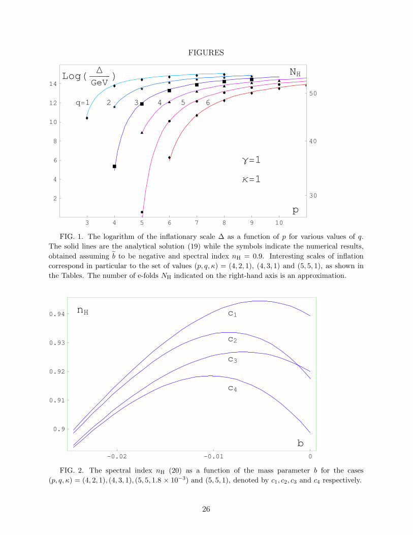
We now present numerical solutions for comparison with the analytical results obtainedabove. First we show in Fig. 1 the dependence of the inflationary scale ∆ on the index p forvarious values of q. The solid lines correspond to the analytical solution (19) showing howaccurately these formulae reproduce the numerical results. Fig. 1 is obtained for negativevalues of b and spectral index nH = 0.9 [18]. We observe that interesting scales for inflationare obtained in particular for the parameter sets (p, q, κ) =(4, 2, 1), (4, 3, 1), (5, 5, 1) and(5, 5, 1.8 × 10−3), as shown in Table I. In Fig. 2 we show the inflationary scale ∆ as afunction of the mass parameter |b| to emphasise its insensitivity to the latter.

9

IV. CHARACTERISTICS OF QUADRATIC INFLATION

Using the form for the potential (13) it is straightforward to determine the propertiesof a wide variety of quadratic inflationary models characterised by the parameters p, q andκ which determine the end of inflation. In what follows we shall usually take κ = 1, its“natural” value and discuss a few representative cases of the discrete possibilities specifiedby the integers p and q. We shall also take the end of inflation to be set by γ = 1, i.e. theepoch when the curvature of the potential becomes unity.

A. The spectral index

The value of nH is shown as a function of the mass parameter |b| in Fig. 3. One cansee that a characteristic property of these models is that the spectral index is boundedas nH

<∼ 0.95 for the cases considered and that for large |b| the index falls rapidly. Oneof the important issues is just how small |b| must be to give acceptable inflation. Thisgives a measure of the severity of the η-problem and will allow us to determine whetherthe candidate explanations presented in Section VB do indeed solve the problem. Usingthe recent observational constraints on nH [18] we can immediately obtain such a limit. InTable I we present these limits assuming nH > 0.8 (0.9).8 We also show the maximum valueof the spectral index nH,max together with the corresponding |b|max for which it is reachedas seen in Fig. 3.

B. Fine tuning measure

Examination of Table I shows that the maximum value of the effective mass squaredparameter b during inflation capable of generating density perturbations in the desired rangeis quite insensitive to the form of the potential at the end of inflation. As we discuss inSection VIB, in non-factorisable higher dimension models the value of b is not constrainedby the value of the inflationary potential so there is no fine tuning implied in this case. Insupersymmetric models the “natural” value of b is ∼ 1 so we see that a fine tuning of about 1part in 20 is required. In our opinion this is rather modest and can easily occur, particularlyin models in which there are several candidate inflaton fields. As discussed in Section VB, itcan happen automatically in various supergravity schemes provided the required reductionin b is relatively modest, namely b >∼ h2/(4π)2 where h is a coupling in the theory. We seethat the required level of fine tuning lies comfortably in this range for reasonable choices ofthe coupling. We conclude therefore that it is quite likely that the necessary conditions forquadratic inflation will be realised in supergravity models. Indeed in realistic models thereare usually a large number of fields associated with flat directions which are candidates for

8The recent Boomerang and MAXIMA observations of small angular-scale CMB anisotropy when

combined with the COBE data indicate nH = 0.89 ± 0.06 if the baryon to photon ratio is fixed at

the value indicated by nucleosynthesis arguments, and nH = 1.01+0.09−0.07 otherwise [18]. The COBE

data alone had previously indicated nH = 1.2 ± 0.3 [4].

10

inflatons. In this case it will be the field with the flattest potential which will generate thelast stage of inflation, the one relevant to our observable universe.

1. Scale of inflation

The scale, ∆, of the inflationary potential during inflation is very sensitive to the form ofthe potential at the end of inflation. However since this form is determined by the discreteparameters p and q, this should not be viewed as fine tuning — a given set will have a definitevalue for ∆ (see Fig. 1). We can see from Table I that a range of ∆ from 1 GeV upwardsis obtained for reasonable choices of p and q. The choice ∆ ≈ 1011 GeV is particularlyinteresting since one can then identify ∆ with the supersymmetry breaking scale in SUGRAmodels in which supersymmetry breaking is communicated from the hidden sector to thevisible sector via gravitational strength couplings. As discussed in Section IIB this value islow enough for thermal effects to set the initial value of the inflaton close to the origin, asis required if one is to have an inflationary era. Much lower values are possible, even downto ∼ 1 GeV and these cases are relevant to the possibility of new large dimensions in whichthere is no fundamental scale much higher than the electroweak scale.

2. The moduli problem

Lowering the scale of the inflationary potential also provides a solution to the moduliproblem. Moduli are scalar fields which, in the absence of symmetry breaking triggeredby non-moduli fields, have no potential i.e. their vevs are undetermined. They are verycommon in string compactification e.g. the dilaton, the complex structure fields, and theirvevs determine the gauge and Yukawa couplings of the theory. There are also moduli whichdetermine the size and shape of the compactification manifold. Because the moduli have avery flat potential they suffer from a “moduli” problem due to the fact that during inflationthe minimum of the moduli potential is typically at a different place from the minimum afterinflation. Thus the moduli fields are trapped at a false minimum during inflation and thisenergy is released after inflation in the form of moduli excitations. If these excitations becomenon-relativistic before they decay into visible sector states they may release a large amountof entropy at a late stage, unacceptably diluting both baryonic and dark matter abundances.The reason the moduli problem may be evaded by lowering the scale of inflation is becausethe distorting effect of the inflation potential is proportional to its magnitude and so reducesas the fourth power of the inflation scale.

To make a quantitative estimate we follow our earlier detailed discussion [8]. First we notethat the distorting contribution to the moduli potential is M2

mm2 where M2

m<∼ V (0)/M2

P;the inequality applies because, as noted for the inflaton, there are various possible ways thesupersymmetry breaking mass scale can be reduced. This is generated by non-perturbativeeffects, such as supersymmetry breaking and may be characterised by Λ4f(m/MP), whereΛ is a symmetry breaking scale. This should now be compared to the inflaton potentialafter inflation. Consider first the case Λ4 < V (0). In this case the moduli are lighter thanthe inflaton and thus decay after the reheating epoch. As discussed earlier [8] this leadsto an unacceptable release of entropy at late times. The problem can be neatly avoided if

11

Λ4 > V (0) for in this case the moduli decay harmlessly releasing their entropy before theinflaton decays.

What is the expectation for Λ? It has been pointed out [8] that for a large class of themoduli, Λ may be identified with the scale of symmetry breaking (triggered by supersymme-try breaking effects) which occur below the string scale. In models with a large intermediatescale of breaking it is quite possible for Λ4 to exceed V (0), even in the case of linear inflationin which V (0) is very large. However at least one modulus, the dilaton, is unaffected by suchintermediate scale breaking and, as it is unlikely that it will get a mass much larger thanthe electroweak scale [19], it will be lighter than the inflaton in linear inflation models andwill lead to an unacceptable late stage of entropy release. However in quadratic inflation

the inflation scale can be very low. Indeed if√V (0)/MP is less than the electroweak scale,

the moduli problem may be solved even for the dilaton. We have seen in Section III that thisis indeed possible.

So far our discussion has been in the context of four-dimensional space-time. If thereare large new dimensions the moduli problem is even more severe because the moduli as-sociated with the size and shape of the new dimensions cannot have mass greater than thefundamental higher dimensional scale of the theory, which may be close to the electroweakscale. The low inflation scale possible in quadratic inflation is essential in these models toavoid the moduli problem for these fields as well.

3. Reheat temperature

One obvious effect of lowering the scale of the inflationary potential is a decrease of thereheat temperature. At the end of inflation the field φ decays reheating the universe. Thecouplings of the inflaton to some other bosonic χ or fermionic ψ MSSM fields occur due toterms −1

2g2φ2χ2 or −hψψφ, respectively. These couplings induce decay rates of the form [1]

Γ(φ→ χχ) =g4φ2

0

8πmφ, Γ(φ→ ψψ) =

h2mφ

8π, (21)

where φ0 ≈ (∆q/κ)1/p is the value of φ at the minimum of the potential, and mφ is theinflaton mass given by

mφ ≈√

2pκ1/p∆2−(q/p). (22)

The decay rate is maximised when mχ,ψ ∼ mφ with Γ ≈ m3φ/8πφ

20. The reheat temperature

at the beginning of the radiation-dominated era is thus [14]

Treh ≈(

90

π2g∗

)1/4

min(√

H(φe)M,√

ΓM)≈(

30

π2g∗

)1/4

min

[∆,(

3

8π2

)1/4

p3/2κ5/2p∆3−5q/2p

].

(23)

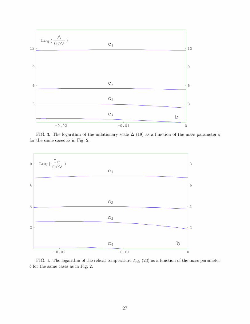
The behaviour of Treh as a function of the mass parameter |b| is shown in Fig. 4. Notethat the observed baryon asymmetry of the universe may in principle be generated afterreheating through anomalous electroweak B+L-violating processes and/or the Affleck-Dinemechanism, even for Treh as low as ∼ 1 GeV [20].

12

So far we have explored the implications of quadratic inflation with a general parameter-isation of the potential, without considering its specific origin. We turn now to a discussionof whether such potentials are reasonable in two attractive classes of models for physicsbeyond the Standard Model.

V. SUPERGRAVITY INFLATION

The only known symmetry capable of solving the hierarchy problem is supersymmetrywhich can guarantee that a scalar mass vanishes in the limit that supersymmetry is unbrokenand ensures, through a cancellation of bosonic and fermionic contributions, that it is notaffected by radiative corrections. However the non-vanishing potential of Eq.(7) drivinginflation breaks (global) supersymmetry and so, even in supersymmetric models, all scalarmasses during inflation are non-zero in general. In the extreme case that the inflaton hasvanishing non-gravitational couplings, gravitational effects will typically induce a mass oforder Hinf ∼ ∆2/M for any scalar field [21], in particular the inflaton [22]. Nevertheless thisis a big improvement over the non-supersymmetric case, for the fine tuning problem nowsimply becomes one of requiring mφ = β∆2/M with β <∼ 0.1 to obtain successful inflation.In this Section we briefly review supergravity models which can lead to this form and discussthe structure of the resulting inflaton potential.

A. The Supergravity potential

In N = 1 supersymmetric theories with a single SUSY generator, complex scalar fieldsare the lowest components, φa, of chiral superfields, Φa, which contain chiral fermions, ψa, astheir other components. In what follows we will take Φa to be left-handed chiral superfields sothat ψa are left-handed massless fermions. Masses for fields will be generated by spontaneoussymmetry breakdown so that the only fundamental mass scale is the normalised Planck scale.This is aesthetically attractive and is also what follows if the underlying theory generatingthe effective low-energy supergravity theory emerges from the superstring. The N = 1supergravity theory describing the interaction of the chiral superfields is specified by theKahler potential [23],

G(Φ,Φ†) = d(Φ,Φ†) + ln |f(Φ)|2. (24)

Here d and f (the superpotential) are two functions which need to be specified; they mustbe chosen to be invariant under the symmetries of the theory. The dimension of d is 2 andthat of f is 3, so terms bilinear (trilinear) in the superfields appear without any mass factorsin d (f). The scalar potential following from Eq.(24) is given by [23]

V = ed/M2

[FA†(dBA)−1FB − 3

|f |2M2

]+D − terms, (25)

where

FA ≡ ∂f

∂ΦA+

(∂d

∂ΦA

)f

M2,

(dBA)−1 ≡

(∂2d

∂ΦA∂Φ†B

)−1

. (26)

13

At any point in the space of scalar fields Φ we can make a combination of a Kahler transfor-mation and a holomorphic field redefinition such that φa = 0 at that point and the Kahlerpotential takes the form d =

∑a |Φa|2 + . . .. In this form, the scalar kinetic terms are canon-

ical at φa = 0 and from Eq.(25), neglecting D-terms and simplifying to the case of a singlescalar field, the scalar potential coming from the F -terms has the form

VF =(e|φ|

2/M2+...) [

|(fφ + fφ∗ + . . .)(1 + . . .)|2 − 3|f |2M2

]= V0 + |φ|2 V0

M2+ . . . , (27)

where V0 ≡ VF |φ=0.

B. Supersymmetry breaking and the η problem

During inflation supersymmetry is broken by the non-zero inflaton potential, V . Forthe case of F -term inflation V0 6= 0 and we see from Eq.(27) that the resultant breaking ofsupersymmetry gives all scalar fields a contribution to their mass-squared of V0/M

2. If thisis the only contribution to the mass there is an obvious conflict with the slow-roll condition(8) on η. This is the essential problem one must solve if one is to implement inflation ina supergravity theory. However, as stressed earlier, the problem is relatively mild whencompared to the non-supersymmetric case because the suppression for η need only be by afactor of 10 or so.

There have been several proposals for dealing with this problem. One widely exploredpossibility is D-term inflation [24]. In particular one may consider an anomalous D-term inEq.(25) of the form

VD =g2

2(ξ −

∑

i

qi|φi|2)2, (28)

where ξ is a constant and φi are scalar fields charged under the anomalous U(1) with chargeqi. Such a term, for vanishing φi, gives a constant term in the potential but, unlike thecase of F -term inflation, VD does not contribute in leading order to the masses of unchargedscalar fields. The latter occur in radiative order only giving a contribution to their mass-squared equal to β2 V0/M

2 where β2 ≈ h′2/16π2, and typically β ≈ 10−1 for an effectivecoupling h′ ∼ 1 between the charged and neutral fields.

The other suggested ways out of the η problem do not require non-zero D-terms duringinflation but rather provide reasons why the quadratic term in Eq.(27) should be anomalouslysmall. One possibility follows from the fact that the mass-squared term of V0/M

2 comingfrom Eq.(27) actually applies at the Planck scale. Since we are considering inflation for fieldvalues near the origin the inflaton mass-squared must be run down to low scales. As shownin Ref. [25], in a wide class of models in which the gauge couplings become large at thePlanck scale the low energy supersymmetry breaking soft masses are driven much smallerat low scales by radiative corrections. The typical effect is to reduce the mass by a factorof α(M)/α(µ) where α(µ) is a gauge coupling evaluated at the scale µ. While radiativecorrections can cause a significant change in the coupling, the effect is limited and becomessmaller as the gauge coupling becomes small. For this reason the effective mass at low scalescannot be arbitrarily small and typically β >∼ 1/25.

14

It is also possible to construct models in which the contribution to the scalar massexhibited in Eq.(27) is cancelled by further contributions coming from the expansion of f inEq.(25). One interesting example which arises in specific superstring theories was discussedin Ref. [26]. Another occurs in supergravity models of the ‘no-scale’ type [27]. In theseexamples, while the scalar mass is absent in leading order, it typically arises in radiativeorder and so again there is an expectation that the effective mass cannot be arbitrarily small.

To summarise, for small inflaton field values, in all these cases the effective supergravitypotential can be conveniently parameterised as a constant term driving inflation plus aquadratic term with coefficient which may be a combination of a “bare” mass at the Planckscale together with a logarithmically varying mass term generated by radiative corrections.Thus the full potential has just the form (12) discussed earlier.

C. Terminating slow-roll evolution

So far we have concentrated on the form of the potential which arises due to supersym-metry breaking effects which inevitably follow from the existence of a non-zero value forthe potential during inflation. However one may expect additional terms in the potentialwhich are allowed even when supersymmetry is unbroken. These terms will determine theposition of the minimum of the potential after inflation and may also be responsible forending inflation.

It is this latter possibility that we shall concentrate on here because the nature of theinflationary era is largely determined by when inflation ends. The reason the end of inflationis likely to be triggered by additional terms in the potential follows from a simple dimensionalargument. In the models we are considering, the inflaton starts with field value close to theorigin and rolls to larger field values. Close to the origin the quadratic terms are likely todominate but as the inflaton field value increases, higher-order terms in φ/M are likely todominate. Such terms may occur through higher-order terms in d or f in Eq.(24) or inhigher-order terms in the expansion of Eq.(27). The form of these terms is restricted byany symmetries (discrete or continuous) of the theory. In compactified string theories suchsymmetries abound, determined by the shape of the compactification manifold. Considerfirst the form of the potential following from the superpotential f . In a string theory, in theabsence of symmetry breaking, the superpotential is cubic in the superfields. In the effectivelow energy theory below the string and compactification scales, higher-order terms may ariseas a result of integrating out heavy modes. The resulting form of the superpotential dependson how the inflaton transforms under the symmetries of the theory. It is not possible togive an exhaustive list of all possible symmetries so here we will consider simple examplesto illustrate the possibilities.

1. Symmetries of the inflaton potential

We start with the case where the inflaton is a singlet under all continuous gauge symme-tries but transforms under a Zq discrete symmetry (which may be a discrete gauge symmetryand thus protected from large gravitational corrections [28]). The leading term in the super-potential is then of the form φq/M q−3 where we have taken the mass scale associated with

15

this term to be the reduced Planck mass, M . (This scale arises as a result of integrating outheavy degrees of freedom associated with the string scale or the compactification scale sohere we are taking all such scales to be of O(M).) Following from Eq.(27) we see that thisterm gives rise to the leading terms of the form |φ|2q−2/M2q−6 in the scalar potential. Notethat this term is not suppressed by the factor ∆4/M2 associated with the quadratic |φ|2 termbecause it arises even in the absence of supersymmetry breaking. This has the importanteffect of reducing the value of φ/M at which the term |φ|2q−2/M2q−6 becomes larger thanthe quadratic term. We see from the slow roll conditions (8) that shortly thereafter thisterm will cause inflation to end. The effect of these higher-order terms may be enhancedstill further if they arise as a result of integrating out heavy modes lighter than the Planckscale. For example the superpotential f = φrX/M r−2 +MXX

2 describes the interaction ofφ with a new field X which has mass MX . The form of this superpotential follows from aZ2r symmetry under which φ and X have charge 1 and r respectively. At scales below MX

the field X may be integrated out to give the effective superpotential f = φ2r/(M2r−4MX).Now the scale of the higher dimension operator is set by a combination of M and MX andfor MX < M will enhance the contribution of the higher dimension term. The new mass MX

could be any of the scales in the theory, e.g. the inflationary scale or the supersymmetrybreaking scale, and can thus be much smaller than the Planck scale.

2. A simple parameterisation

With this preamble we now consider how to parameterise the structure of the termsresponsible for ending inflation. Consider first the inflationary models driven by a non-zeroF -term. This is conveniently parameterised by the superpotential f = ∆2Y which givesV = |FY |2 = ∆4 as required. Radiative corrections then lead to the form of Eq.(12). Asdiscussed above we expect higher-order corrections involving the inflaton to appear and thereare many possible forms for such corrections depending on the underlying symmetries of thetheory. Here we present a convenient parameterisation of the potential which follows froma simple symmetry to demonstrate how a complete inflation potential may be driven by thesymmetry structure. The starting point is the superpotential f = ∆2Y . Such a form linearin Y follows if Y carries non-zero R-symmetry charge 2β under an unbroken R-symmetrybecause the full superpotential must also have charge 2β under such a symmetry. Now let φbe a singlet under the R-symmetry but have a charge under a discrete Zp symmetry. Thenthe most general superpotential has the form

f =

(∆2 − φp

M ′p−2− φ2p

M ′2p−2− . . .

)Y, (29)

where we have suppressed the coefficients of O(1) of each term. This gives rise to thepotential

V =

(∆2 − φp

M ′p−2− φ2p

M ′2p−2− . . .

)2

, (30)

plus terms involving Y which we drop as they do not contribute to the vacuum energy(since Y does not acquire a vacuum expectation value). For small φ the leading term has

16

the form ∆2φp/M ′p−2 and, for the purpose of ending inflation, this is all that matters —the higher-order terms in Eq.(30) do not play a role during inflation. Thus this form ofthe superpotential gives the same inflationary phenomenology as discussed in the previoussubsection with the superpotential φq/M q−3, provided the leading higher-order terms inφ are the same, i.e. p = 2q − 2 and M = M ′(M ′/∆)1/(q−3). This illustrates the moregeneral point that different symmetries may lead to the same inflationary potential. For ourparameterisation we use a slightly simplified form of Eq.(30) keeping only the leading φp

term and setting M ′p−2 = ∆q−2Mp−q to take account of the possibility discussed above thatthe scale associated with the higher dimension operators may be below the Planck scale.Note q is an integer as the term ∆q comes from heavy propagators when integrating outmassive fields. Thus we arrive at the form

V = ∆4

(1 − κ

φp

∆qMp−q

)2

+ ∆4

b(|φ|M

)2

+ c ln

(|φ|M

)(|φ|M

)2 , (31)

where we have added the supersymmetry breaking terms of Eq.(12). As discussd earlier,this form of the inflationary potential allows for a variety of inflationary scales ∆ dependingon the choice of p and q and our results for the potential (13) in Table I should apply withthe interpretation b = b+ c lnφ2

H. In Table II we show the results of a numerical integrationof the potential (31), demonstrating that this is indeed the case. To conclude this discussionwe show in detail how the symmetries lead to the higher-order term φp/M ′p−2 = ∆q−2Mp−q

in the superpotential for three representative cases, identifying the origin of the mass scaleM ′ and hence the source of the ∆q factor.

• Case 1: p = 4, q = 2, ∆ ≈ 1011 GeV

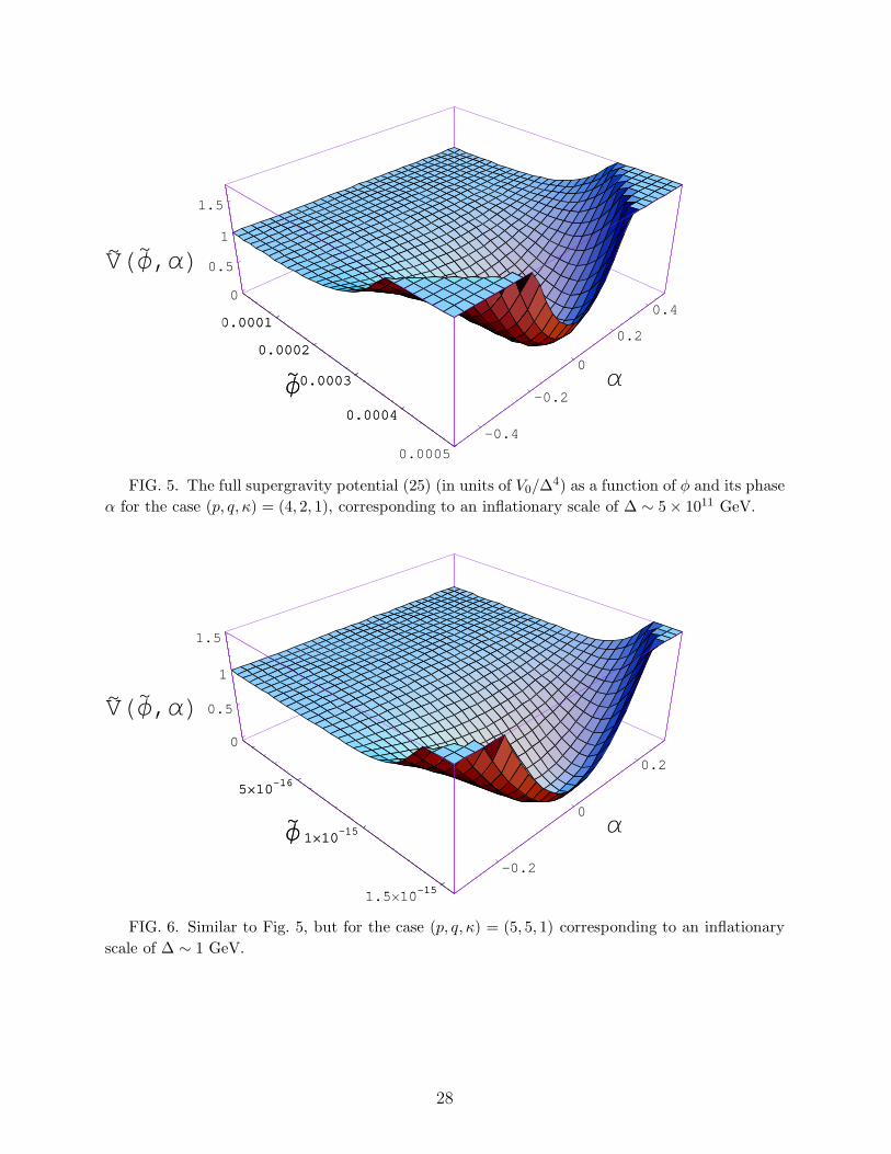
This simple case follows immediately from a Z4 symmetry under which φ has unitcharge and Y is neutral. Taken together with the R-symmetry the leading term allowedis Y φ4/M2 whereM is the fundamental mass scale of the theory which we take to be thePlanck scale. Combined with the supersymmetry breaking term Y∆2 we immediatelyobtain Eq.(31) with p = 4, q = 2. As discussed above, this potential gives acceptabledensity perturbations provided ∆ ≈ 1011 GeV, i.e. it can be identified with thesupersymmetry breaking scale. Fig. 5 shows the full supergravity inflaton potential(25) as a function of φ and its phase α for (p, q, κ) = (4, 2, 1).

• Case 2: p = 4, q = 3, ∆ ≈ 105 GeV

In this case we choose the superpotential of the form

f = Y φX +MXXX +Xφ3/M. (32)

This form arises if there is a U(1) (or Zn) symmetry under which the fields Y,X,X, φhave charge -4, 3, -3 and 1 respectively. Integrating out the massive X,X fields gives

f = Y φ4/(MMX). (33)

If MX = ∆ (as is expected if X,X belong to the supersymmetry breaking sectordriven by a gaugino condensate in which the (confining) interactions become strong

17

at the scale ∆) we have the desired term in the superpotential which, when combinedwith the supersymmetry breaking term Y∆2 (the SUSY breaking condensate, ∆2, alsobreaks the U(1) (or Zn) symmetry), yields the form given in Eq.(31).

• Case 3: p = 5, q = 5, ∆ ≈ 1 GeV

This is readily achieved along similar lines to the previous case via the superpotential

f = Y φ2Z + ZX2 + Xφ2 +MZZZ +MXXX (34)

This form arises if there is a U(1) (or Zn) symmetry under which the fieldsY, Z, Z,X,X, φ have charge -10, 8, -8, 4, -4 and 2 respectively. Integrating out themassive X,X fields gives

f = Y φ5/M2XMZ (35)

With MX=MZ=∆ and the supersymmetry breaking term Y∆2 we arrive at a super-potential giving Eq.(31) with p = 5, q = 5. Fig. 6, similar to Fig. 5, but now for(p, q, κ) =(5, 5, 1), shows how lower scales of inflation require lower values of φ; inparticular we see how the minimum φ0 shifts to smaller values.

3. D-term inflation

So far we have discussed the form of the inflaton potential responsible for ending inflationthat may arise as a result of F -term inflation. However it is possible to obtain similarforms using D-term inflation and, as noted in Section VB, this may have the advantage ofeliminating the η problem. At first sight it seems impossible to obtain D-term inflation witha low scale for the inflationary potential because the usual assumption is that the non-zerovalue of the D-term is due to an anomalous U(1) as in Eq.(28) and its scale is in turn relatedto the string scale. However there are two possible ways that a low D-term scale may arise.The first possibility is that the string scale itself is low. With the realisation that the four-dimensional Planck scale may not be a fundamental quantity has come the construction ofstring models with low string scales (even as low as ∼ 1 TeV) plus large new dimensions.In these theories the weakness of the gravitational interactions is due to the gravitationalflux spreading out in new large extra space dimensions or through the appearance of a warpfactor in the 4-D metric dependent on the additional dimensions. Either way the string scaleand hence the associated anomalous D-term is reduced. The second possibility applies evenin the original string formulations with small extra dimensions. The fields in the hiddensupersymmetry breaking sector all feel the strong confining force responsible for gauginocondensation. Such fields may be driven to acquire vevs of the order of the scale ∆ atwhich the force becomes strong. These vevs may give rise to non-zero D-terms capable ofgenerating inflation at the scale ∆. Given these possibilities what is the form of the potentialand does it have similar properties to that of Eq.(31)? In both of the cases just discussedthe general form of the D-term is given by

VD =∣∣∣|∆|2 −X†X +X

†X∣∣∣2, (36)

18

where we have included fields X and X carrying +1 and -1 charge respectively under theU(1) gauge symmetry. The end of D-term inflation must be driven in a different mannerfrom that discussed above, namely through hybrid inflation. During inflation the X field isprevented from acquiring a vev because it has a mass, MX , which we take to come from thesupersymmetry breaking sector and hence to be of O(∆). The end of inflation correspondsto the point at which the change in the vev of the inflaton, φ , which is a singlet underthe gauge symmetry associated with the non-zero D-term, must alter the potential of X insuch a way that it can acquire a vev cancelling the D-term. The most general form of thesuperpotential is (suppressing Yukawa couplings)

f = MXXX + φXX + higher − order terms (37)

The potential following from this includes the leading terms

VF = |MX + φ|2 (|X|2 +∣∣∣X∣∣∣2) +

∣∣∣XX∣∣∣2. (38)

For φ ≈ 0 the X field has mass MX and for MX>∼ ∆ the potential VD + VF will constrain

X to have zero vev. Once the vev of φ becomes of O(MX) however a cancellation of the Xmass term is possible and the X field will rapidly evolve so as to minimise VD. Since the Xmass scale is >∼ ∆ this happens within a Hubble time and so inflation is effectively ended.In fact for MX of O(∆) this reproduces Case 1 discussed above because there too the end ofinflation occurred at φ of O(∆). Variations on this hybrid theme can readily generate theother cases too. Replacing the φX term in Eq.(37) by the term φsXX/∆t (such a term canbe obtained by integrating out fields in an analogous way to that discussed above) one finds

inflation ends for φ = (∆tMX)1/s

. For the potential of the form given in Eq.(31) the end ofinflation occurs at φ ≈ ∆q/(p−2) and so for MX of O(∆) and q/(p− 2) = (t+ 1)/s, the endof inflation will be the same in the D-term case.

VI. 4-D INFLATION IN HIGHER DIMENSION THEORIES

As mentioned above there has recently been much interest in a solution to the hierarchyproblem involving δ new large dimensions in which gravity (described by closed strings ina string theory) propagate in the 4 + δ dimensions while the matter states of our world,quarks, leptons and the gauge bosons responsible for the strong, weak and electromagneticinteractions, (described by open string states whose ends are confined to D-branes) live injust the normal four-dimensional space (the D=3 case). The description of inflation in morethan 4 dimensions may be done either by using the full higher dimensional description orby using an effective 4-D description in which the effects of the higher dimension appearas towers of Kaluza Klein states. Which description is more appropriate depends on theenergy scale of interest. Here we use the four-dimensional description because it is verylikely that during inflation the effective temperature drops below the compactification scaleat which the extra dimensions are frozen. Even if inflation starts at a scale above thecompactification scale for the additional dimensions, during inflation the universe cools to

the Hawking temperature ∼√V (0)/M , and, if this is below the compactification scale, the

theory will be effectively four-dimensional during inflation. If this is not the case we expect

19

problems because the phase transition corresponding to compactification will occur after

inflation. While this is not necessarily “no-go”, it is rather disfavoured since the modulisetting the scale of the new dimensions propagate in the additional dimensions and arelikely to produce an unacceptable amount of entropy in the bulk.

In the effective 4-D description, it is necessary to discuss how the presence of additionallarge dimensions may change the form of the slow-roll equations.

A. Factorisable metric

In the original realisation of this idea [29] one assumes a factorisable metric of the form

ds2 = −dx0dx0 + dxidxi + dxαdx

α, i = 1, 2, 3, α = 4, . . . , 4 + δ , (39)

and finds that, due to the gravitational flux leaking out into the extra dimensions, thegravitational coupling to matter in 4-D is much weaker than in the higher dimensionalspace, with the 4-D Planck mass given by

M2P,4 = M δ+2

P,4+δ Rδ. (40)

Thus provided MP,4+δ R ≫ 1, one can explain why the four-dimensional Planck mass islarge while the fundamental mass scale MP,4+δ remains small. In the extreme one may takeMP,4+δ of O(1) TeV), i.e. small enough to eliminate the hierarchy problem which occurswhen one introduces scales much larger than the electroweak scale. In such theories thereis no mass scale higher than MP,4+δ. Moreover the reheat temperature must be extremelylow [29] if the bulk is not to contain so much energy that it distorts the expansion rate ofthe universe in an unacceptable way. Given this it is clear that the only viable inflationarymodel is one which does not require a high scale for the inflaton potential, pointing atquadratic inflation as the obvious candidate. Moreover it is necessary for the theory still tobe supersymmetric in order to explain why the inflaton mass is only of order the Hubbleexpansion parameter during inflation (i.e. the inflation sector supersymmetry breaking scale)— without supersymmetry one expects it would be driven to the scale MP,4+δ. Thus thediscussion about the form of the inflation potential in supersymmetric theories applies tofactorisable metric compactifications as well. The important difference is that in Eq.(31)M should be identified with MP,4+δ and not with the 4-D Planck mass. At first sight thisdoes not seem to be the correct prescription because the inflaton, a brane state, has onlygravitational strength couplings ∝ M−n

P,4 to the new Kaluza Klein states responsible for theadditional dimensions in our 4-D description. However after summing over all the KaluzaKlein states these couplings do induce higher-order corrections ∝ φn+4/Mn

P,4+δ.

B. Non-factorisable metric

Recently there has been renewed interest in the case where the metric is not factorisable.For the case of a single extra dimension the line element has the form

ds2 = e−ρ(r)(−dx0dx0 + dxidxi) + dx4dx

4, i = 1, 2, 3, (41)

20

where x4 = rθ, 0 < θ ≤ 2π. The origin of the hierarchy between the electroweak breakingscale and the Planck scale is now rather different than that suggested for the factorisablemetric case. An explicit example was recently provided by Randall and Sundrum [30].They considered the case of two parallel 3-branes sitting on the fixed points of an S1/Z2

orbifold. The 5-D spacetime is essentially a slice of five-dimensional Ant-DeSitter space-time and the tensions of the two 3-branes are chosen so that the 4-D spacetime appearsflat. This last requirement forces one of the two branes to have negative tension. Thesolution to Einstein’s equations now has the form of Eq.(41) with ρ(r) = kR where k is thefive-dimensional curvature. The exponential “warp” factor, = e−kR, in the metric thengenerates a hierarchy of the mass scales between the two branes, although all fundamentalmass scales are of order MP,4. The graviton is localised to the positive tension brane whilematter exists on the negative tension brane with particle masses of order MP,4. Due tothe exponential dependence of the warp factor on the size of the new dimension, one mayreadily generate the desired mass hierarchy with ∼ 10−1 even though the size, R, of theorbifold is only ∼ 30 times k−1 which is of order the Planck length.

It may seem that such schemes have a great advantage in generating slow-roll inflationby easily solving the η-problem. This follows because these models provide a reason whythe inflaton mass should be less than the Hubble parameter during inflation even without

supersymmetry. The reason is that, due to the universal warp factor, all masses on a givenbrane involve the warp factor suppression. As we have just discussed this is why on thevisible brane all masses are of order the electroweak breaking scale. If the inflaton lives onthe visible brane (or a brane very close to it) it too will have an electroweak scale masswhich is stable against radiative corrections from sectors on other branes. In this schemethere should be vacuum energy, V (0), (the net contribution from the bulk and the branes)driving inflation until the inflaton rolls to its minimum to cancel the vacuum energy. Unlikethe factorisable case there is no constraint on the fundamental higher-dimensional scale. Asa result V (0) can be large, even as large as the 4-D Planck scale. Thus, in this case, bothlinear and quadratic inflation appear viable even without supersymmetry.

However, if V (0) is much greater than the scale, Λ, on the inflaton brane, the inflatonwill not be able to cancel V (0) fully. This is because to cancel V (0) the inflaton vev mustbe of order V (0)1/4. However above the scale Λ on the inflaton brane the underlying higher-dimension theory (string theory?) must be used because the effective theory has uncontrolledhigher-dimension terms of the form φn/Λn−4. Thus even in this case we need a mechanismto ensure that the inflaton is anomalously light to satisfy the slow-roll equations (8). Theobvious candidate is supersymmetry as already discussed.

Up to now this discussion has been at a qualitative level. To be more explicit we considerthe five-dimensional case in which the Standard Model states and the inflaton live on a 3-brane while gravity propagates in the full five dimensions. We start with the 5-D description.Solution of the Einstein equations for the case that the metric is projected on to a spatiallyflat Friedmann-Robertson-Walker (FRW) model and the 4-D cosmological constant afterinflation is set to zero gives a modified form for the Hubble expansion rate [32–34]

H2 =8π

3M24

ρ(1 +

ρ

2λ

), (42)

where λ is the brane tension, ρ is the energy density and we have used M4 to denote MP,4.It is given by

21

M4 =

√3

4π

(M2

5√λ

)M5, (43)

where M5 = MP,5. In Eq.(42) the term quadratic in ρ corrects the standard FRW cosmology.However the effective 4-D Lagrangian should have just the Einstein-Hilbert form and onemight expect to recover the standard cosmology. In fact this is the case, provided the Planckconstant appearing therein is time dependent.9 It is easy to see this during inflation whenρ = V (φ). Expanding the potential about the point where density perturbations leave thehorizon we find

H2 =1

3M24

V (0)

(1 +

V (0)

2λ

)(1 + V ′(0)φ+

1

2V ′′(0)φ2 + . . .

),

where we have dropped terms of O(φ/λ). One can see that this has just the normal 4-Dform but with a modified Planck mass

M ′24 = M2

4

(1 +

V (0)

2λ

)−1

. (44)

The case of chaotic (large-field) inflation (i.e. linear inflation in our terminology) has beenexplored in Ref. [35]. In this case, for M5 ≪M4, the new term quadratic in V in Eq.(42) islarge, so the modified Planck mass is reduced with

M ′24 ≃ 104M2

5 .

As a result, following the discussion leading to Eq.(3), we see that linear inflation generatesthe correct magnitude of density perturbations with the scale

V (0)1/4 ≃ 2√cM5, (45)

which can be low for M5 low. Indeed in the chaotic inflationary model investigated [35] thescale of inflation is ∼ M5/10. This demonstrates a new mechanism for generating low-scaleinflation without requiring quadratic inflation or supersymmetry, which is apparently inconflict with the general arguments given above!

To explain this we note that Eq.(44) relies on the variation of the Planck scale between theperiod perturbations are produced and today, the variation corresponding to the variationof the horizon size. This will not be the case for compact extra dimensions [30] if inflationoccurs after the size of the extra dimensions are fixed because the horizon then is bigger

than the compactification radius. As argued above, we consider this to be the likely case ifthe bulk is to remain empty. In this case the Planck mass does not differ during and afterinflation and, following the arguments above, one sees that linear inflation requires the scaleof inflation to be as large as in Eq.(3). As a result, if one is to have a low inflationary scaleconsistent with a low fundamental scaleM5 on the brane, it is necessary to consider quadraticinflation. Moreover, as discussed above, it is then also necessary to invoke supersymmetry to

9We are grateful to A. Karch for helpful comments concerning this point.

22

keep the coefficient of the quadratic term below the Hubble rate as required by the slow-rollconditions (8).

For the case that the additional dimensions are infinite [31] the result of Eq.(45) is apossibility, the variation of the Planck scale corresponding to the variation of the horizon.The new ingredient is that there is no new compact dimension and furthermore the Planckscale is time-dependent. However even in this case there are reasons why one needs su-persymmetric quadratic inflation. We note that the specific chaotic inflation model of ref.[35] requires an inflaton mass m ≃ 5 × 10−5M5 and thus there must be supersymmetryor some other mechanism responsible to keep the inflaton mass much less than its naturalscale M5, as noted earlier [36]. Moreover even this is not sufficient to make linear low-scaleinflation viable. The value of the inflaton vev at the time perturbations are produced isφ′ ∼ 3×102M5. Since non-renormalisable quantum corrections occur at O(φ′n+4/Mn

5 ), suchlarge values of the inflaton field are likely to destroy the flatness of the potential requiredfor inflation. Indeed, as discussed above, for φ′ above M5 it is necessary to use the under-lying (string?) theory which is needed to regulate the O(φ′n+4/Mn

5 ) terms. For the caseof quadratic inflation these problems need not arise because the scale of the inflationarypotential, V (0), can be much smaller than the brane tension λ so, c.f. Eq.(42), the form ofthe inflationary potential at the time the observable perturbations are produced is just thenormal 4-D one analysed in Section II.

VII. SUMMARY

In this paper we have explored the possibility that there could be an inflationary era as-sociated with a low scale for the inflationary potential. The most extensively studied modelscorrespond to the case where the inflaton potential is linear in a Taylor expansion about thevalue of the inflaton field just before the time when the observable density perturbations areproduced. In these models the scale of inflation is restricted to lie close to the Planck scaleby the requirement that scalar density perturbations should have their observed magnitude.On the other hand, models in which the inflaton potential is quadratic have density pertur-bations which depend sensitively on the value of the inflaton field at the end of inflation.We have explored the implications of such models in detail and found they can generateacceptable perturbations even if the scale of inflation is the electroweak scale or even lower.

Low scale inflation has several attractive features. It offers a solution to the troublesomemoduli problem associated with superstring compactification. At least in the context of su-persymmetric theories, thermal effects readily impose the required initial conditions neededfor such inflation to occur. If there are large new space dimensions solving the hierarchyproblem, a low scale of inflation is essential as there are no large fundamental mass scales.

The construction of a viable inflationary model requires an explanation as to why theinflaton potential should be much flatter than dimensional arguments using the fundamentalmass scale of the theory would suggest. The most promising solution is if there is anunderlying supersymmetry which maintains the flatness of the inflaton potential even in thepresence of a large (supersymmetry breaking) cosmological (near) constant term. Simplesupersymmetric models readily lead, through large non-renormalisable terms, to the rapidend of inflation needed to achieve low scale inflation. We have also considered the possibilityfor low scale inflation in models with large new dimensions. Although these models offer

23

an alternative non-supersymmetric explanation for the hierarchy problem they still requirean additional mechanism to keep the inflaton potential flat, again suggesting the need forsupersymmetry.

Determining the nature of the underlying theory leading to inflation is a difficult task.The forthcoming precision CMB and LSS measurements will certainly play an importantrole in this and we have seen that low scale quadratic inflationary models give a character-istic prediction (‘tilted’ or ‘red’) for the spectral index of the scalar density perturbation.Laboratory experiments will play a complementary role because the implication of an un-derlying supersymmetry is that there should be new supersymmetric states which are likelyto be observable in the next generation of experiments. Thus there is a good chance thatthe ideas investigated in this paper may be tested within the next decade.

ACKNOWLEDGMENTS

GG gratefully acknowledges financial support from the Royal Society and the MexicanAcademy of Sciences, which made possible a visit to the University of Oxford; he alsoacknowledges support by UNAM project PAPIIT IN110200. GGR would like to thank theAspen Institute of Physics, where part of this work was undertaken (supported by TMRgrant FMRX-CT96-0090) and P. Binetruy, A. Karch, R. Maartens and L. Randall for usefuldiscussions.

24

TABLES

p q κ nH nH,max |b| |b|max ∆ (GeV) ∆max (GeV)

4 2 1 0.8 (0.9) 0.95 0.05 (0.024) 0.005 7(46)×1010 50×1010

4 3 1 0.8 (0.9) 0.93 0.05 (0.024) 0.007 4.6(27)×104 28.7×104

5 5 1 0.8 (0.9) 0.92 0.05 (0.024) 0.01 1.3(4.2) 2.9

5 5 1.5×10−3 0.8 (0.9) 0.94 0.05 (0.024) 0.008 1(10)×102 7.6×102

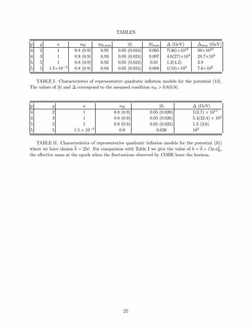
TABLE I. Characteristics of representative quadratic inflation models for the potential (13).

The values of |b| and ∆ correspond to the assumed condition nH > 0.8(0.9).

p q κ nH |b| ∆ (GeV)

4 2 1 0.8 (0.9) 0.05 (0.026) 1(3.7) × 1011

4 3 1 0.8 (0.9) 0.05 (0.026) 5.4(22.4) × 104

5 5 1 0.8 (0.9) 0.05 (0.025) 1.3 (3.6)

5 5 1.5 × 10−3 0.9 0.026 103

TABLE II. Characteristics of representative quadratic inflation models for the potential (31)

where we have chosen b = 25c. For comparison with Table I we give the value of b = b + c ln φ2H,

the effective mass at the epoch when the fluctuations observed by COBE leave the horizon.

25

FIGURES

3 4 5 6 7 8 9 10

2

4

6

8

10

12

14

30

40

50

p

LogHD���������GeVL NH

q=1 2 3 4 5 6

Γ=1

Κ=1

FIG. 1. The logarithm of the inflationary scale ∆ as a function of p for various values of q.

The solid lines are the analytical solution (19) while the symbols indicate the numerical results,

obtained assuming b to be negative and spectral index nH = 0.9. Interesting scales of inflation

correspond in particular to the set of values (p, q, κ) = (4, 2, 1), (4, 3, 1) and (5, 5, 1), as shown in

the Tables. The number of e-folds NH indicated on the right-hand axis is an approximation.

-0.02 -0.01 0

0.9

0.91

0.92

0.93

0.94

b

nH c1

c2

c3

c4

FIG. 2. The spectral index nH (20) as a function of the mass parameter b for the cases

(p, q, κ) = (4, 2, 1), (4, 3, 1), (5, 5, 1.8 × 10−3) and (5, 5, 1), denoted by c1, c2, c3 and c4 respectively.

26

-0.02 -0.01 0

3

6

9

12

3

6

9

12

b

LogHD�����������GeV

Lc1

c2

c3

c4

FIG. 3. The logarithm of the inflationary scale ∆ (19) as a function of the mass parameter b

for the same cases as in Fig. 2.

-0.02 -0.01 0

2

4

6

8

2

4

6

8

b

LogHTrh�����������GeV

L

c1

c2

c3

c4

FIG. 4. The logarithm of the reheat temperature Treh (23) as a function of the mass parameter

b for the same cases as in Fig. 2.

27

0.0001

0.0002

0.0003

0.0004

0.0005

Φ�

-0.4

-0.2

0

0.2

0.4

Α

0

0.5

1

1.5

V�HΦ�,ΑL

0.0001

0.0002

0.0003

0.0004

0.0005

Φ�

FIG. 5. The full supergravity potential (25) (in units of V0/∆4) as a function of φ and its phase

α for the case (p, q, κ) = (4, 2, 1), corresponding to an inflationary scale of ∆ ∼ 5 × 1011 GeV.

5´10-16

1´10-15

1.5´10-15

Φ�

-0.2

0

0.2

Α

0

0.5

1

1.5

V�HΦ�,ΑL

5´10-16

1´10-15

1.5´10-15

Φ�

FIG. 6. Similar to Fig. 5, but for the case (p, q, κ) = (5, 5, 1) corresponding to an inflationary

scale of ∆ ∼ 1 GeV.

28

REFERENCES

[1] A.D. Linde, Particle Physics and Inflationary Cosmology (Harwood Academic, 1990);E.W. Kolb and M.S. Turner, The Early Universe (Addison-Wesley, 1990).

[2] D. Lyth, A. Riotto, Phys. Rep. 314 (1999) 1.[3] J.E. Lidsey, A.R. Liddle, E.W. Kolb, E.J. Copeland, T. Barreiro, M. Abney, Rev. Mod.

Phys. 69 (1997) 373[4] C.L. Bennett et al, Astrophys. J. 464 (1996) L1;

E.F. Bunn, M. White, Astrophys. J. 486 (1997) 6.[5] A.D. Linde, Phys. Lett. 129B (1983) 177.[6] A.D. Linde, Phys. Lett. 132B (1983) 317.[7] A.D. Linde, Phys. Lett. 108B (1982) 389;

A. Albrecht, P.J. Steinhardt, Phys. Rev. Lett. 48 (1982) 1220.[8] G.G. Ross, S. Sarkar, Nucl. Phys. B461 (1996) 597.[9] T. Vachaspati, M. Trodden, Phys. Rev. D61 (2000) 023502;

A. Berera, C. Gordon, Phys. Rev. 63 (2001) 063505.[10] P.J. Steinhardt, in The Very Early Universe, eds G.W. Gibbons, S.W. Hawking, S. Sik-

los (Cambridge University Press, 1982), p. 251;A.D. Linde, Nonsingular Regenerating Inflationary Universe, Cambridge University Re-port Print-82-0554 (1982);A. Vilenkin, Phys. Rev. D27 (1983) 2848;A. Guth and S.-Y. Pi, Phys. Rev. D32 (1985) 1899;A. Linde, D. Linde, A. Mezhlumian, Phys. Rev. D49 (1994) 1783;A. Linde and D. Linde, Phys. Rev. D50 (1994) 2456.

[11] S.W. Hawking, N. Turok, Phys. Lett. B425 (1998) 25;A. Vilenkin, Phys. Rev. D57 (1998) 7069;A.D. Linde, Phys. Rev. D58 (1998) 083514;N. Turok, S.W. Hawking, Phys. Lett. B432 (1998) 271;For a review, see, N. Turok, astro-ph/0011195.

[12] J.A. Adams, G.G. Ross, S. Sarkar, Nucl. Phys. B503 (1997) 405.[13] J. Barriga, E. Gaztanaga, M.G. Santos, S. Sarkar, Mon. Not. R. Astr. Soc., to appear

(astro-ph/0011398).[14] P.J. Steinhardt, M.S. Turner, Phys. Rev. D29 (1984) 2162.[15] G. German, G.G. Ross, S. Sarkar, Phys. Lett. 469B (1999) 46.[16] K. Enqvist, J. Sirkka, Phys. Lett. B314 (1993) 298;[17] K. Enqvist, K.J. Eskola, Mod. Phys. Lett. A5 (1990) 1919.[18] A.H. Jaffe et al, Phys. Rev. Lett. 86 (2001) 3475.[19] T. Banks, M. Berkooz, P.J. Steinhardt, Phys. Rev. D52 (1995) 705;

T. Banks et al, Phys. Rev. D52 (1995) 3548.[20] see, e.g., S. Davidson, M. Losada, A. Riotto, Phys. Rev. Lett. 84 (2000) 4284.[21] M. Dine, W. Fischler, D. Nemechansky, Phys. Lett. 136B (1984) 169;

G. Coughlan, W. Fischler, E.W. Kolb, S. Raby, G.G. Ross, Phys. Lett. 140B (1984) 44.[22] E. Copeland, A.R. Liddle, D.H. Lyth, E.D. Stewart, D. Wands, Phys. Rev. D49 (1994)

6410.[23] D. Bailin, A. Love, Supersymmetric Gauge Field Theory and String Theory (Adam

Hilger, 1994).

29

[24] E.D. Stewart, Phys. Rev. D51 (1995) 6847;E. Halyo, Phys. Lett. B387 (1996) 43;P. Binetruy, G. Dvali, Phys. Lett. B388 (1996) 241;For a review and further references, see Ref. [2].

[25] S.F. King, G.G. Ross, Nucl. Phys. B530 (1998) 3.[26] J.A. Casas, G.B. Gelmini, Phys. Lett. B410 (1997) 36;

J.A. Casas, G.B. Gelmini, A. Riotto, Phys. Lett. B459 (1999) 91.[27] M.K. Gaillard, H. Murayama, K.A. Olive, Phys. Lett. B355 (1995) 71;

M. Bastero-Gil, S.F. King, Nucl.Phys. B549 (1999) 391.[28] L.E. Ibanez, G.G. Ross, Nucl. Phys. B368 (1992) 3, Phys. Lett. B260 (1991) 291.[29] N. Arkani-Hamed, S. Dimopoulos, G. Dvali, Phys. Lett. B429 (1998) 263.[30] L. Randall, R. Sundrum, Phys. Rev. Lett. 83 (1999) 3370.[31] L. Randall, R. Sundrum, Phys. Rev. Lett. 83 (1999) 4690.[32] T. Shiromizu, K. Maeda, M. Sasaki, Phys. Rev. D62 (2000) 024012;

P. Binetruy, C. Deffayet, U. Ellwanger, D. Langlois, Phys. Lett. B477 (2000) 285.[33] P. Kanti, I. Kogan, K. Olive, M. Pospelov, Phys. Lett. B468 (1999) 31, Phys. Rev D61

(2000) 106004;T. Nihei, Phys. Lett. B465 (1999) 81;N. Kaloper, Phys. Rev. D60 (1999) 123506;C. Csaki, M. Graesser, C. Kolda, J. Terning, Phys. Lett. B462 (1999) 34;J.M. Cline, C. Grojean, G. Servant, Phys. Rev. Lett. 83 (1999) 4245.

[34] H.B. Kim, H.D. Kim, Phys. Rev. D61 (2000) 064003;E.E. Flanagan, S.H. Tye, I. Wasserman, Phys. Rev. D62 (2000) 044039.

[35] R. Maartens, D. Wands, B. Bassett, I. Heard, Phys. Rev. D62 (2000) 041301.[36] D.H. Lyth, Phys. Lett. B448 (1999) 191.

30