Maximum moduli of unimodular polynomials

J. Korean Math. Soc. 41 (2004), No. 1, pp. 209–229

MAXIMUM MODULI OFUNIMODULAR POLYNOMIALS

Andreas Defant, Domingo Garcıa and Manuel Maestre

Abstract. LetP|α|=m sαzα, z ∈ Cn be a unimodular m-homoge-

neous polynomial in n variables (i.e. |sα| = 1 for all multi indicesα), and let R ⊂ Cn be a (bounded complete) Reinhardt domain. Wegive lower bounds for the maximum modulus supz∈R |

P|α|=msαzα|,

and upper estimates for the average of these maximum modulitaken over all possible m-homogeneous Bernoulli polynomials (i.e.sα = ±1 for all multi indices α). Examples show that for a fixeddegree m our estimates, for rather large classes of domains R, areasymptotically optimal in the dimension n.

0. Introduction

In his study [5] of Dirichlet series∑∞

n=1anns Harald Bohr considered

vertical strips of uniform, but not absolute convergence of such a se-ries. More precisely, he considered those nonnegative numbers A andB for which a given Dirichlet series

∑∞n=1

anns converges conditionally

(i.e., absolutely) in the half plane s ∈ C : Re s > A, but con-verges uniformly on the half planes s ∈ C : Re s ≥ B + ε, ε > 0.Bohr asked for the maximal possible width d := B − A of such a strip,and proved that d ≤ 1

2 . Bohnenblust and Hille in [6] were able toshow that d = 1

2 . In the context of nuclearity and absolute bases forspaces of holomorphic functions over infinite dimensional domains, Di-neen and Timoney in [14] gave a new proof based on probabilistic meth-ods. Finally, Boas in a beautiful paper [2] produced a proof in whichone of the key ingredients is the Kahane-Salem-Zygmund Theorem (see

Received December 17, 2002.2000 Mathematics Subject Classification: Primary 32A05; Secondary 46B07,

46B09, 46G20.Key words and phrases: several complex variables, power series, polynomials, Ba-

nach spaces, unconditional basis, Banach-Mazur distance.The second and third authors were supported by MCYT and FEDER Project

BFM2002-01423.

210 Andreas Defant, Domingo Garcıa and Manuel Maestre

[18, Theorem 4, Chap. 6, pp.70–71]). This probabilistic result, foreach degree m and each dimension n, assures the existence of an m-homogenous Bernoulli polynomial P (z) =

∑|α|=m sαzα on Cn for which

sup|P (z)| : |zk| < 1, k = 1, . . . , n ≤ Cnm+1

2√

log m, where C de-pends neither on n nor on m. A similar argument was used by Boas andKhavinson [3, proof of Theorem 2] in their study of Bohr’s power seriestheorem in several variables (see also [1], [9] and [13]).

The main goal of this paper is to give, in a systematic way, upper andlower estimates for the maximum modulus supz∈R |

∑|α|=m sαzα|, where∑

|α|=m sαzα is an arbitrarily given m-homogeneous Bernoulli polyno-mial in n variables (i.e., a polynomial of the form

∑|α|=m sαzα, where

the coefficients sα for all α are signs) and R some Reinhardt domain inCn. In section 2 we obtain for every unimodular m-homogeneous poly-nomial (i.e., every polynomial of the form

∑|α|=m sαzα, z ∈ Cn, where

sα ∈ C satisfies |sα| = 1 for all multi indices α) and every Reinhardt do-main R lower bounds for the maximum modulus supz∈R |

∑|α|=m sαzα|.

In section 3 we give upper estimates for the average of such maximummoduli taken over all possible m-homogeneous Bernoulli polynomials.As a consequence we prove for certain classes of domains the existenceof m-homogeneous Bernoulli polynomials which have maximum modulias small as possible. Moreover, we apply our results to various concreteclasses of domains R in Cn.

1. Preliminaries

We shall use standard notation and notions from Banach space theoryas presented e.g. in [22] or [28]. If X is a Banach space over the scalarsK = R or C, then X∗ is its topological dual and BX is its open unit ball.We denote the Banach-Mazur distance of two Banach spaces X and Yby d(X, Y ).

For all needed background on polynomials defined on Banach spaceswe refer to [12] and [16]. P(mX) denotes the space of all m-homogeneousscalar valued polynomials P on a Banach space X, which together withthe norm ‖P‖ := sup|P (x)| : ‖x‖ ≤ 1 forms a Banach space. Asubset U of Cn is called circled if λx ∈ U for all λ ∈ C, |λ| = 1. Acomplete bounded Reinhardt domain R ⊂ Cn is a bounded domainthat is complete and n-circled, i.e. if x = z1e1 + · · · + znen ∈ R, thenλ(eθ1iz1e1 + · · ·+eθniznen) ∈ R for all λ ∈ C, |λ| ≤ 1 and all θ1, . . . , θn ∈R. A basis (xn) of a Banach space X is said to be unconditional if there is

Maximum moduli of unimodular polynomials 211

a constant C ≥ 1 such that for all µ1, . . . , µn ∈ K and all s1, . . . , sn ∈ Kwith |sk| ≤ 1, we have ||∑n

k=1 skµkxk|| ≤ C||∑nk=1 µkxk||; in this case

the best constant is denoted by χ((xn)), the unconditional basis constantof (xn). All unconditional bases considered in this paper are normalized.For X = (Kn, ‖.‖) denote by χmon(P(mX)) the unconditional basis con-stant of the monomials zα : |α| = m.

We call a Banach space X = (Kn, ‖.‖) symmetric if the canonicalvectors ek form a symmetric basis, i.e. ‖x‖ = ‖∑n

k=1 skxπ(k)ek‖ foreach x ∈ X, each permutation π of 1, . . . , n and each choice of scalarssk with |sk| = 1. A Banach space X for which `1 ⊂ X ⊂ c0 (withnorm 1 inclusions) is said to be a Banach sequence space if the canon-ical sequence (ek) forms a 1-unconditional basis; it is called symmetricif ‖x‖ = ‖∑∞

k=1 skxπ(k)ek‖ for each x ∈ X, each permutation π of Nand each choice of scalars sk with |sk| = 1. Recall finally that a Banachlattice X is said to be 2-concave and 2-convex, respectively, if there isa constant C > 0 such that

( ∑nk=1 ‖xk‖2

)1/2 ≤ C‖( ∑nk=1 |xk|2

)1/2‖,and ‖(∑n

k=1 |xk|2)1/2‖ ≤ C

(∑nk=1 ‖xk‖2

)1/2 for all x1, . . . , xn ∈ X, re-spectively. Here the best constant is denoted by M(2)(X) and M (2)(X),respectively (see [22]). For the notion of cotype q, 2 ≤ q < ∞, of a Ba-nach space X (the cotype constant is denoted by Cq(X)) and its relationwith convexity and concavity we also refer to [22].

2. Lower bounds for the maximum modulus of unimodularhomogeneous polynomials on Reinhardt domains

Fix a degree m and a dimension n. We call an m-homogeneous poly-nomial

(2.1)∑

|α|=m

sαzα, z ∈ Cn

unimodular whenever all coefficients sα ∈ C satisfy |sα| = 1. If allsα ∈ C are signs +1 and −1, then we speak of an m-homogeneousBernoulli polynomial. Obviously,

supz∈B`n∞

|∑

|α|=m

sαzα| ≤∑

|α|=m

|sα| =(

n + m− 1m

).

Conversely, since the monomials zα, |α| = m, form an orthogonal systemof square integrable functions on the n-dimensional torus Tn in Cn (the


n-th cartesian product of S`12endowed with the product measure of the

normalized Lebesgue measure σ1), we get(

n + m− 1m

)1/2

=( ∫

Tn

|∑

|α|=m

sαzα|2dz)1/2

≤ supz∈B`n∞

|∑

|α|=m

sαzα|≤(

n + m− 1m

).

(2.2)

Hence, the obvious estimate 1m!n

m ≤ (n+m−1

m

) ≤ nm gives

(2.3)1√m!

nm/2 ≤ supz∈B`n∞

|∑

|α|=m

sαzα| ≤ nm.

Let us improve the lower bound. We want to show that there is a con-stant cm > 0 such that for each unimodular m-homogeneous polynomialas in (2.1)

(2.4) cmnm+1

2 ≤ supz∈B`n∞

|∑

|α|=m

sαzα|.

We are going to obtain this lower estimate as a consequence of thefollowing more general result.

Proposition 2.1. Let X = (Cn, ‖.‖) be a Banach space such thatthe canonical basis (ek)n

k=1 is 1-unconditional. Then for each m

(2.5)1m!

(supz∈BX

∑nk=1 |zk|

)m

χmon(P(mX))≤ sup

z∈BX

|∑

|α|=m

sαzα|.

Proof. For each unimodular m-homogeneous polynomial∑

|α|=m

sαzα, z ∈ Cn

we have(

supz∈BX

n∑

k=1

|zk|)m =

(sup

z∈BX

|n∑

k=1

zk|)m

= supz∈BX

|∑

|α|=m

m!α1! · · ·αn!

zα|


= supz∈BX

|∑

|α|=m

m!α1! · · ·αn!sα

sαzα|

≤ m!χmon(P(mX)) supz∈BX

|∑

|α|=m

sαzα|.

By [8, Theorem 3] we know that for each m there is a constant dm > 0such that

(2.6) χmon(P(m`n∞)) ≤ dmn

m−12 .

As nm =(supz∈B`n∞

∑nk=1 |zk|

)m, inequality (2.6) together with Propo-sition 2.1 gives as desired (2.4) with cm := (m!dm)−1. In contrast to (2.6)we know that χmon(P(m`n

1 )) for fixed degree m is uniformly boundedfrom above in the dimension n (see [9, (4.6)]), more precisely

χmon(P(m`n1 )) ≤ mm

m!.

Hence by Proposition 2.1 we have

(2.7)1

mm≤ sup

z∈B`n1

|∑

|α|=m

sαzα|,

i.e., for each fixed degree m the maximum modulus of a unimodularm-homogeneous polynomial on B`n

1is uniformly bounded from below in

n.More generally, we now prove a theorem which includes (2.4) and

(2.7) as particular cases. We will need the following lemma which isrelated to [3, Theorem 3] and [13, Theorem 3.2].

Lemma 2.2. Given r1, . . . , rn > 0, consider on Cn the norm ‖z‖ :=sup| zk

rk| : k = 1, . . . , n and denote the associated Banach space by

`n∞(r1, . . . , rn). Then

χmon(P(m`n∞(r1, . . . , rn))) ≤ dmn

m−12 ,

where the constant dm > 0 is the one from (2.6).

Proof. Clearly the open unit ball of `n∞(r1, . . . , rn) is the polydisc z ∈Cn : |zk| < rk, k = 1, . . . , n. Let

∑|α|=m cαzα be an m-homogeneous

polynomial on Cn such that

|∑

|α|=m

cαzα| ≤ 1, for all z ∈ B`n∞(r1,...,rn).


Then|

∑

|α|=m

cα(rkzk)α| ≤ 1, for all z ∈ B`n∞ ,

which implies

|∑

|α|=m

cαrαzα| ≤ 1, for all z ∈ B`n∞ .

Hence, we obtain by (2.6) that

|∑

|α|=m

|cα|rαzα| ≤ dmnm−1

2 , for all z ∈ B`n∞ ,

which finally gives as desired that

|∑

|α|=m

|cα|zα| ≤ dmnm−1

2 , for all z ∈ B`n∞(r1,...,rn).

The following result is our main lower bound for maximum moduliof unimodular m-homogeneous polynomials.

Theorem 2.3. For each m there is a constant cm > 0 such that foreach unimodular m-homogeneous polynomial

∑|α|=m sαzα, z ∈ Cn the

following estimates hold.

(1) For each Reinhardt domain R ⊂ Cn

cm

(supz∈R

∑nk=1 |zk|

)m

nm−1

2

≤ supz∈R

|∑

|α|=m

sαzα|.

(2) For each Banach space X := (Cn, ‖.‖) for which the e′ks form a1-unconditional basis

cm

(supz∈BX

∑nk=1 |zk|

)m

d(X, `n1 )m−1

≤ supz∈BX

|∑

|α|=m

sαzα|.

(3) If, additionally, BX ⊂ B`n2

we obtain

cm supz∈BX

n∑

k=1

|zk| ≤ supz∈BX

|∑

|α|=m

sαzα|.

Proof. Each Reinhardt domain R is, by definition, a union of openpolydiscs. Given u ∈ R, we take r1, . . . , rn > 0 such that u ∈ z ∈ Cn :


|zk| < rk, k = 1, . . . , n ⊂ R. By Proposition 2.1 and Lemma 2.2 thereis a constant cm > 0 for which

cm(∑n

k=1 |uk|)m

nm−1

2

≤ cm

(supz∈B`n∞(r1,...,rn)

∑nk=1 |zk|

)m

nm−1

2

≤ supz∈B`n∞(r1,...,rn)

|∑

|α|=m

sαzα| ≤ supz∈R

|∑

|α|=m

sαzα|,

and hence (1) is proved. Statement (2) follows from Proposition 2.1 andthe fact that by [9, Theorem 6.1] there exists a constant dm > 0 suchthat

(2.8) χmon(P(mX)) ≤ dmd(X, `n1 )m−1;

now it is enough to take cm := (m!dm)−1. The proof of (3) is a conse-quence of the fact that by [26, Corollary 2] and [9, (5.2)]:

1√2

supz∈BX

n∑

k=1

|zk| ≤ d(X, `n1 ) ≤ sup

z∈BX

n∑

k=1

|zk|.

This completes the proof.

Let us collect some concrete examples in order to illustrate our re-sults.We start with estimates for mixed Minkowski spaces

ùp(`v

q) := (xk)uk=1 : x1, . . . , xu ∈ Cv

‖(xk)uk=1‖p,q := (

u∑

k=1

‖xk‖pq)

1/p.

Example 2.4. Let∑|α|=m sαzα, z ∈ Cu(Cv) be a unimodular m-

homogeneous polynomial in uv variables (for some order of these vari-ables). Then

supz∈Bù

p (`vq )

|∑

|α|=m

sαzα| ≥ C

um+1

2−m

p vm+1

2−m

q if 2 ≤ p, q ≤ ∞,

u1− 1

p v1− 1

q if 1 ≤ p, q ≤ 2,

u1− 1

p vm+1

2−m

q if 1 ≤ p ≤ 2 ≤ q ≤ ∞,

C > 0 some constant depending only on m, p and q.


Let us remark that, by taking p = q and v = 1 in this example, we ob-tain lower estimates for every unimodular m-homogeneous polynomialson `n

p , 1 ≤ p ≤ ∞:

(2.9) supz∈B`n

p

|∑

|α|=m

sαzα| ≥ C

nm+1

2−m

p if 2 ≤ p ≤ ∞,

n1− 1

p if 1 ≤ p ≤ 2 .

The results of the next section will show in which sense these esti-mates are optimal. Our proof of Example 2.4 needs the following

Lemma 2.5. In the three cases 1 ≤ p, q ≤ 2 or 2 ≤ p, q ≤ ∞ or1 ≤ p ≤ 2 ≤ q ≤ ∞ we have

d(ùp(`v

q), ùv1 ) ≤ d(ù

p , ù1)d(`v

q , `v1).

Proof. For 1 ≤ p, q ≤ 2 we know from [26, Corollary 2] that

d(ùp(`v

q), ùv1 ) ≤ ‖

∑

k,l

ek ⊗ el‖ùp′ (`

vq′ )

= u1− 1

p v1− 1

q = d(ùp , ù

1)d(`vq , `

v1);

see e.g. [28, 37.6]. If 2 ≤ p, q ≤ ∞, then M (2)(ùp(`v

q)) = 1, and hence itfollows from [28, Corollary 41.9] that as desired

d(ùp(`v

q), ùv1 ) ≤ C

√uv,

C ≥ 0 some absolute constant. Finally, the remaining case: Note firstthat for every linear bijection T : `v

q −→ `v1

d(ù1(`v

q), ùv1 ) = d(ù

1 ⊗π `vq , `

u1 ⊗π `v

1) ≤ ‖id⊗T‖‖id⊗T−1‖ = ‖T‖‖T−1‖,hence d(ù

1(`vq), `

uv1 ) ≤ d(`v

q , `v1); for 1 ≤ p ≤ 2 ≤ q ≤ ∞ now by factor-

izationd(ù

p(`vq), `

uv1 ) ≤ d(ù

p(`vq), `

u1(`v

q))d(ù1(`v

q), ùv1 )

≤ ‖id : ùp(`v

q) −→ ù1(`v

q)‖d(`vq , `

v1)

= u1−1/pd(`vq , `

v1) ≤ d(ù

p , ù1)d(`v

q , `v1).

For the remaining case 1 ≤ q ≤ 2 ≤ p ≤ ∞ the estimate from Lemma2.5 is false; by a result of Kwapien and Schutt from [20, Corollary 3.3]we, e.g., see that d(`n∞(`n

1 )), `n2

1 )n³ n (and not, as one could expect

from the estimate of the lemma,√

n). We believe that at least in thisspecial case the optimal lower bound for supz∈B`n∞(`n

1 ))|∑|α|=m sαzα|

comes from Theorem 2.3(1), namely nm+1

2 .


Proof of the Example 2.4. All three cases are consequences of Theo-rem 2.3. We know that

supz∈Bù

p (`vq )

∑

k,l

| < z, ek ⊗ el > | = ‖id : ùp(`v

q) −→ ùv1 ‖ = u1−1/pv1−1/q.

Hence the first case is a consequence of Theorem 2.3(1), the second oneof 2.3(3), and the last of 2.3(2) combined with the preceding lemma.

The next example deals with Orlicz spaces `ϕ, and is a considerableextension of (2.9) (take ϕ(t) = tp).

Example 2.6. Let ϕ be an Orlicz function satisfying the ∆2-condi-tion. Then for each m there is a constant cm > 0 such that for eachunimodular m-homogeneous polynomial

∑|α|=m sαzα in n variables, the

following estimates hold.

(1) cmnm+1

2 ϕ−1(1/n)m ≤ supz∈B`ϕ|∑|α|=m sαzα|.

(2) cmnϕ−1(1/n) ≤ supz∈B`ϕ|∑|α|=m sαzα|, provided that t2≤ Kϕ(t)

for all t and some K.

Proof. The proof is again a simple consequence of Theorem 2.3, theobservations (3.5) and (3.6) (anticipated from section 3), combined withthe well-known equality ‖∑n

k=1 ek‖`ϕ = 1ϕ−1(1/n)

for the fundamentalfunction; the condition in (2) assures that `ϕ ⊂ `2.

We finish this section with an example for a non-convex domain.

Example 2.7. Given S > 1 and n ≥ 2 consider the Reinhardt domainR := (z1, . . . , zn) ∈ Cn : |z1 · · · zn| < 1 , |zk| < S, k = 1, . . . , n. Thenfor each m there exists a constant hm > 0 such that for all unimodularm-homogeneous polynomials

∑|α|=m sαzα in n variables

hmSmnm+1

2 ≤ supz∈R

|∑

|α|=m

sαzα|.

Proof. We have that

(2.10) supz∈R

n∑

k=1

|zk| = (n− 1)S +1

Sn−1;

indeed, if we take the compact set K := x ∈ [0, S]n : x1 · · ·xn ≤ rfor 0 < r ≤ 1, then the maximum of the function f(x) := x1 + · · · +xn on K is (n − 1)S + r

Sn−1 , attained at (S, . . . , S, rSn−1 ) and at any

point whose coordinates are a permutation of it. Let x0 ∈ K suchthat f(x0) = supx∈K f(x). As f has no critical points, x0 belongs to


∂K, the boundary of K. On the other hand x0 does not belong tox ∈ (0, S)n : x1 · · ·xn = r. In this case the Lagrange multipliermethod gives only the critical point (r1/n, . . . , r1/n). But the functiong : (0,∞) −→ R defined by g(x) := (n − 1)x + r

xn−1 attains a strictabsolute minimum at x = r1/n and

f(r1/n, . . . , r1/n) = nr1/n = g(r1/n)

< g(S) = (n− 1)S +r

Sn−1= f(S, . . . , S,

r

Sn−1).

If x ∈ ∂K and for some k we have xk = 0, then f(x) ≤ (n − 1)S <f(S, . . . , S, r

Sn−1 ) and x 6= x0. Finally, the only possibility left is that forsome k we have xk = S. Then, by the symmetry of the function f , wecan assume xn = S. By induction, we have

sup(x1, . . . , xn−1) ∈ [0, S]n−1 : x1 · · ·xn−1 ≤ rS−1 = (n−2)S+rS−1

Sn−2,

thusf(x1, . . . , xn−1, S)

≤ S + sup(x1, . . . , xn−1) ∈ [0, S]n−1 : x1 · · ·xn−1 ≤ rS−1= (n− 1)S +

r

Sn−1= f(S, . . . , S,

r

Sn−1).

Now, since supz∈R

∑nk=1 |zk| coincides with the maximum of f on

x ∈ [0, S]n : x1 · · ·xn ≤ 1, we obtain the equality (2.10). Hence, byTheorem 2.3 (1) there exists a constant cm > 0 such that

cm1

2mSmn

m+12 ≤ cm

(n− 1n

)mSmn

m+12 ≤ cm

((n− 1)S + 1

Sn−1

)m

nm−1

2

≤ supz∈R

|∑

|α|=m

sαzα|.

The conclusion follows by taking hm = cm1

2m .

3. Expectations of the modulus maximum of homogeneousBernoulli random polynomials on Reinhardt domains

The Kahane-Salem-Zygmund Theorem [18, Theorem 4, Chap. 6,pp.70–71] shows that for the polydisc typically the maximum modulus

supz∈B`n∞

|∑

|α|=m

sαzα|


of an arbitrarily given unimodular m-homogeneous polynomial is assmall as possible, namely n

m+12 (see (2.4)). To obtain polynomials on

`np with “small” norms Boas in [1, Theorem 4] proves the existence of

symmetric complex m-linear forms on (`np )m with “small” norms. His

proof, as explicitly stated, is made by a careful inspection of results dueto Mantero-Tonge (see [23, Theorem 1.1] and also [24, Proposition 4])which in turn were inspired by the Kahane-Salem-Zygmund Theorem.This section could be considered as an extension of the Mantero-Tongeresults. It is worth to mention that [23, Theorem 1.1] was used byDineen and Timoney in [13] and [14].

Let us clarify what we mean by “ small” norm. Fix a degree m, afamily εα : Ω → −1, 1, |α| = m of independent Bernoulli randomvariables on a probability space (Ω, µ) (each εα takes the values +1 and−1 with equal probability 1/2), and cα ∈ C. Then we call

∑

|α|=m

cαεαzα, z ∈ Cn ,

an m-homogeneous Bernoulli random polynomial. According to [18,Chapter 6, Theorem 3] there is an absolute constant C > 0 such that

µ(

supz∈B`n∞

|∑

|α|=m

εαzα| ≥ Cnm+1

2 (log m)1/2) ≤ 1

m2en.

Hence with “ high probability” the maximum modulus of every m-ho-mogeneous Bernoulli polynomial

∑|α|=m sαzα, z ∈ Cn , can be esti-

mated from above by a constant times (log m)1/2nm+1

2 ; in particular,there exists a set of signs sα, |α| = m such that

supz∈B`n∞

|∑

|α|=m

sαzα| ≤ C(log m)1/2nm+1

2 .

To see from another point of view that (2.4) for fixed m is optimal in thedimension n, integrate (2.4) in order to obtain the following lower esti-mate for the expectation of the modulus maximum of an m-homogeneousBernoulli random polynomial with respect to the polydisc B`n∞ :

cmnm+1

2 ≤∫

Ωsup

z∈B`n∞

|∑

|α|=m

εαzα|dµ ;

by [9, Corollary 6.5] we know that this result is optimal. More generally,given a Reinhardt domain R in Cn satisfying one of the assumptions of


Theorem 2.3, integration gives a lower bound for the averages∫

Ωsupz∈R

|∑

|α|=m

εαzα|dµ ,

and a modification of [9, Theorem 3.1] will show that for rich classes ofdomains R the lower bounds obtained in this way, are optimal.

Recall that a real valued random variable X on a probability space(Ω, µ) is said to be Gaussian whenever it has mean zero, is square inte-grable and its Fourier transform satisfies

EeitX = e−‖X‖22

2t2 , where t ∈ R and ‖X‖2 = (EX2)

12 ;

X is a standard Gaussian random variable if it is measurable and if forevery Borel subset B of R we have

µω ∈ Ω : g(ω) ∈ B =1√2π

∫

Be−

t2

2 dt .

The following result is our main technical tool.

Theorem 3.1. Let U be a bounded circled set in Cn, and (gα)|α|=m

and (gk)1≤k≤n two families of independent standard Gaussian randomvariables on a probability space (Ω, µ). Then for each choice of scalarscα, |α| = m

∫supz∈U

|∑

|α|=m

cαgαzα|dµ

≤ Cm sup|α|=m

|cα|

√α!m!

supz∈U

(n∑

k=1

|zk|2)m−1

2

∫supz∈U

|n∑

k=1

gkzk|dµ,

where 0 ≤ Cm ≤ 232m− 1

2 m32 .

Since the proof is a simple modification of [9, Theorem 3.1] we onlysketch some relevant details. In fact, we prove a reformulation whichneeds some more notation. For natural numbers m,n we defineM(m,n):= 1, . . . , nm and J (m,n) := j = (j1, . . . , jm) ∈ 1, . . . , nm : j1 ≤· · · ≤ jm. Moreover, for j ∈ J (m,n) let |j| be the cardinality of theset of all i ∈ M(m,n) for which there is a permutation τ of 1, . . . , nsuch that iτ(k) = jk for 1 ≤ k ≤ m. Finally, if e∗k denotes the kthcoefficient functional on Cn and j ∈ J (m, n), then we write e∗j (z) :=e∗j1(z) · · · e∗jm

(z), z ∈ Cn. Now observe that if α ∈ (N ∪ 0)n is a multiindex such that |α| = m, then zα = zα1

1 · · · zαnn = e∗j (z) for all z ∈ Cn,


where j = (α1−times

1, . . . . . . , 1, . . . ,αn−times

n, . . . . . . , n), and that in this case |j| = m!α! .

Hence, the following inequality is a reformulation of Theorem 3.1:∫supz∈U

|∑

j∈J (m,n)

cjgje∗j (z)|dµ

≤ Cm supj∈J (m,n)

|cj|√|j| sup

z∈U(

n∑

k=1

|zk|2)m−1

2

∫supz∈U

|n∑

k=1

gkzk|dµ.

(3.1)

The crucial ingredient of the proof of Theorem 3.1 is Slepian’s lemma.Given N real-valued random variables Xk : Ω → R,

(X1, . . . , XN ) : Ω → RN

is said to be a Gaussian random vector provided that each real linearcombination

∑Nk=1 αkXk is Gaussian. For example, if each Xk itself

is a real linear combination of standard Gaussians, then they form aGaussian random vector. The following comparison theorem originatesin the work of Slepian [25] (see Fernique [15], and also [17, Remark1.5] and [21, Corollary 3.14]): let (X1, . . . , XN ) and (Y1, . . . , YN ) beGaussian random vectors such that E|Yi − Yj |2 ≤ E|Xi −Xj |2 for eachpair (i, j). Then

(3.2) Emaxi

Yi ≤ Emaxi

Xi.

Proof of inequality (3.1). Without loss of generality we may assumethat all coefficients cj are real, and |cj| ≤

√|j| for all j ∈ J (m,n). The

aim is to estimate instead of the average∫supz∈U

|∑

j∈J (m,n)

cjgje∗j (z)|dµ ,

for each finite set D ⊂ U , the average

(3.3)∫

supz∈D

∑

j∈J (m,n)

cjgjRe e∗j (z)dµ.

Indeed, if P is an m-homogeneous polynomial on Cn, then it is veryeasy to prove, by the fact that U is circled and P is homogeneous, that‖P‖ = supz∈U ReP (z). Since, by hypothesis, cj ∈ R and gj : Ω −→ Rfor all j ∈ J (m,n), for each w ∈ Ω

supz∈U

|∑

j∈J (m,n)

cjgj(w)e∗j (z)| = supz∈U

∑

j∈J (m,n)

cjgj(w)Re e∗j (z).


Moreover, by a compactness argument for each ε > 0 there is a finitesubset D ⊂ U such that

∫supz∈U

∑

j∈J (m,n)

cjgj(w)Re e∗j (z)dµ

≤∫

supz∈D

∑

j∈J (m,n)

cjgj(w)Re e∗j (z)dµ + ε.

If now αl2m−1

l=1 is an ordering of α : α = (αu)mu=1 ∈ 0, 1m such that

m− |α| is even, then for every j ∈ J (m, n) and z ∈ Cn,

Re e∗j (z) =2m−1∑

l=1

εlal,1j1

(z) · · · al,mjm

(z),

where al,uk (z) := Re e∗k(z)αl

uIm e∗k(z)1−αlu and εl := (−1)(m−|αl|)/2, 1 ≤

l ≤ 2m−1, 1 ≤ u ≤ m and 1 ≤ k ≤ n. Define the following two Gaussianrandom processes:

Yz :=∑

j∈J (m,n)

cjgj(w)Re e∗j (z)

=∑

j∈J (m,n)

cjgj

2m−1∑

l=1

εlal,1j1

(z) · · · al,mjm

(z), z ∈ Cn,

Xz :=2m−1∑

l=1

m∑

u=1

n∑

k=1

gl,u,kal,uk (z), z ∈ Cn,

where the gj, gl,u,k and gk all stand for independent standard Gaussianrandom variables. Note that for fixed l and u, the term

∑nk=1 gl,u,ka

l,uk (z)

coincides either with∑n

k=1 gl,u,kRe e∗k(z) or with∑n

k=1 gl,u,kIm e∗k(z) forall z ∈ Cn. Fix now a finite set D ⊂ U , and show exactly as in the proofof [9, Theorem 3.1] that for each pair x, y in D

(∫|Yx − Yy|2dµ)1/2

≤√

2m−1√

m supz∈U

(n∑

k=1

|zk|2)m−1

2 (∫|Xx −Xy|2dµ)1/2.


By Slepian’s lemma (3.2) we finally obtain∫

supz∈D

∑

j∈J (m,n)

cjgjRe e∗j (z)dµ

≤√

2m−1√

m supz∈U

(n∑

k=1

|zk|2)m−1

2

∫supz∈D

2m−1∑

l=1

m∑

u=1

n∑

k=1

gl,u,kal,uk (z)dµ

≤√

2m−1√

m supz∈U

(n∑

k=1

|zk|2)m−1

2

2m−1∑

l=1

m∑

u=1

∫supz∈D

∣∣n∑

k=1

gl,u,kzk

∣∣dµ

=√

2m−1√

m 2m−1m supz∈U

(n∑

k=1

|zk|2)m−1

2

∫supz∈D

∣∣n∑

k=1

gkzk

∣∣dµ.

Together with the consideration from (3.3) this completes the proof.

Estimating Bernoulli by Gaussian averages, we add an explicit esti-mate of the expectation of the maximum modulus of an m-homogeneousBernoulli random polynomial.

Corollary 3.2. Let (εα)|α|=m and (εk)1≤k≤n be a families of in-dependent standard Bernoulli random variables on a probability space(Ω, µ), and let cα, |α| = m be scalars.

(1) For each bounded circled set U in Cn we have∫

supz∈U

|∑

|α|=m

cαεαzα|dµ

≤√

log nCm sup|α|=m

|cα|

√α!m!

supz∈U

(n∑

k=1

|zk|2)m−1

2 supz∈U

n∑

k=1

|zk|.

(2) Let X = (Cn, ‖.‖) be a Banach space for which the ek’s form an1-unconditional basis, and let 2 ≤ q < ∞. Then we have∫

supz∈BX

|∑

|α|=m

cαεαzα|dµ

≤ c√

qCq(X∗) Cm sup|α|=m

|cα|

√α!m!

sup

z∈BX

(n∑

k=1

|zk|2)m−1

2 supz∈BX

n∑

k=1

|zk|.

Here c > 0 is an absolute constant and Cm as above.

Proof. We use the following facts:


(i) Gauss averages in a Banach space always dominate Bernoulli av-erages (see e.g. [28, (4.2), p.15]),

(ii) given a Banach space Y and y1, . . . , yn ∈ Y , then∫‖

n∑

k=1

gkyk‖Y dµ ≤√

log n

∫‖

n∑

k=1

εkyk‖Y dµ

(see e.g. [28, (4.4) p.15]),(iii) there is a constant c > 0 such that, given a Banach space Y of

cotype q, for each choice of y1, . . . , yn ∈ Y , we have∫‖

n∑

k=1

gkyk‖Y dµ ≤ c√

qCq(Y )∫‖

n∑

k=1

εkyk‖Y dµ

(see e.g. [28, (4.3) p.15]), where (gk), respectively (εk), is a family of in-dependent standard Gaussian, respectively Bernoulli, random variableson a probability space. Now from (i), (ii) and Theorem 3.1 we obtain∫

supz∈U

|∑

|α|=m

cαεαzα|dµ

≤√

log nCm sup|α|=m

|cα|

√α!m!

supz∈U

(n∑

k=1

|zk|2)m−1

2

∫supz∈U

|n∑

k=1

εkzk|dµ.

But

(3.4)∫

supz∈U

|n∑

k=1

εkzk|dµ ≤∫

supz∈U

n∑

k=1

|zk|dµ = supz∈U

n∑

k=1

|zk| ,

which proves (3.2). (3.2) follows from (i), (iii), Theorem 3.1 and (3.4).

Given m ∈ N, if (an(m))∞n=1 and (bn(m))∞n=1 are scalar sequences wewrite an(m)

m³ bn(m) whenever there are some cm, dm > 0 such thatcman(m) ≤ bn(m) ≤ dman(m) for all n. Again we illustrate our resultsby several examples. The first example is the counterpart of Example2.4.

Example 3.3.

∫sup

z∈Bùp (`v

q )

|∑

|α|=m

εαzα|dµm³

um+1

2−m

p vm+1

2−m

q if 2 ≤ p, q ≤ ∞,

u1− 1

p v1− 1

q if 1 < p, q ≤ 2,

u1− 1

p vm+1

2−m

q if 1 < p ≤ 2 ≤ q ≤ ∞.


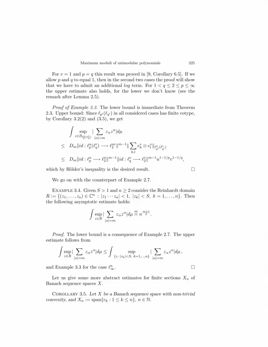
For v = 1 and p = q this result was proved in [9, Corollary 6.5]. If weallow p and q to equal 1, then in the second two cases the proof will showthat we have to admit an additional log term. For 1 < q ≤ 2 ≤ p ≤ ∞the upper estimate also holds, for the lower we don’t know (see theremark after Lemma 2.5).

Proof of Example 3.3. The lower bound is immediate from Theorem2.3. Upper bound: Since `p′(`q′) in all considered cases has finite cotype,by Corollary 3.2(2) and (3.5), we get

∫sup

z∈Bùp (`v

q )

|∑

|α|=m

εαzα|dµ

≤ Dm‖id : ùp(`v

q) −→ ùv2 ‖m−1‖

∑

k,l

e∗k ⊗ e∗l ‖ùp′ (`

vq′ )

≤ Dm‖id : ùp −→ ù

2‖m−1‖id : `vq −→ `v

2‖m−1u1−1/pv1−1/q,

which by Holder’s inequality is the desired result.

We go on with the counterpart of Example 2.7.

Example 3.4. Given S > 1 and n ≥ 2 consider the Reinhardt domainR := (z1, . . . , zn) ∈ Cn : |z1 · · · zn| < 1, |zk| < S, k = 1, . . . , n. Thenthe following asymptotic estimate holds:

∫supz∈R

|∑

|α|=m

εαzα|dµm³ n

m+12 .

Proof. The lower bound is a consequence of Example 2.7. The upperestimate follows from

∫supz∈R

|∑

|α|=m

εαzα|dµ ≤∫

supz : |zk|<S, k=1,...,n

|∑

|α|=m

εαzα|dµ ,

and Example 3.3 for the case `n∞.

Let us give some more abstract estimates for finite sections Xn ofBanach sequence spaces X.

Corollary 3.5. Let X be a Banach sequence space with non-trivialconvexity, and Xn := spanek : 1 ≤ k ≤ n, n ∈ N.


(1) For each m there is a constant Dm > 0 such that for every n

1Dm

(supz∈BXn

∑nk=1 |zk|

)m

nm−1

2

≤∫

supz∈BXn

|∑

|α|=m

εαzα|dµ ≤ Dm supz∈BXn

(n∑

k=1

|zk|2)m−1

2 supz∈BXn

n∑

k=1

|zk|.

(2) If X is symmetric and 2-convex, then∫

supz∈BXn

|∑

|α|=m

εαzα|dµm³

(supz∈BXn

∑nk=1 |zk|

)m

nm−1

2

.

(3) If X ⊂ `2, then∫

supz∈BXn

|∑

|α|=m

εαzα|dµm³ sup

z∈BXn

n∑

k=1

|zk|.

This result is an improvement of [9, Corollary 6.5].

Proof. The lower bound in (1) is a consequence of Theorem 2.3 (1).Since X∗ has non-trivial concavity, which implies that it has cotype q forsome 2 ≤ q < ∞ , the upper bound in (1) is a consequence of Corollary3.2 (2). In (2) it remains to show the upper bound: We may assumethat M (2)(X) = 1, hence

supz∈BXn

(n∑

k=1

|zk|2)1/2 =supz∈BXn

∑nk=1 |zk|√

n

(see [27, Proposition 2.2] and [11, Proposition 3.5]). Hence, the con-clusion in (2) is a consequence of the upper bound in (1). Finally, theupper bound in (3) follows from the upper bound in (1), and the lowerbound in (3) by Theorem 2.3 (3).

In the symmetric case the above three statements can be reformulatedin terms of the fundamental function ‖∑n

k=1 ek‖Xn , n ∈ N of X:

Remark 3.6. Let X be a symmetric Banach sequence space withnon-trivial convexity, and Xn := spanek : 1 ≤ k ≤ n, n ∈ N.

(1’) For each m there is a constant Dm such that for every n

1Dm

nm+1

2

‖∑nk=1 ek‖m

Xn

≤∫

supz∈BXn

|∑

|α|=m

εαzα|dµ ≤ Dm‖id : Xn −→ `n2‖m−1 n

‖∑nk=1 ek‖Xn

.


(2’) If X is 2-convex, then∫

supz∈BXn

|∑

|α|=m

εαzα|dµm³ n

m+12

‖∑nk=1 ek‖m

Xn

.

(3’) If X ⊂ `2, then∫sup

z∈BXn

|∑

|α|=m

εαzα|dµm³ n

‖∑nk=1 ek‖Xn

.

Proof. The proof easily follows from the following observations:

supz∈BXn

(n∑

k=1

|zk|2)1/2 = ‖id : Xn −→ `n2‖

supz∈BXn

n∑

k=1

|zk| = ‖n∑

k=1

e∗k‖X∗n

= ‖id : Xn −→ `n1‖,

(3.5)

and the well known fact that for symmetric X for all n

(3.6) n = ‖n∑

k=1

e∗k‖X∗n‖

n∑

k=1

ek‖Xn

(see [22, Proposition 3.a.6, p.118, vol. I]).

In our Corollaries 3.2 and 3.5 and Examples 3.3 and 3.4 we haveproved upper bounds for the average of the maximum moduli of m-homogenous Bernoulli random polynomials. This shows the existenceof m-homogeneous Bernoulli polynomials which have norms being lessor equal to the bounds given in these results. Moreover, in section 2for some cases (see e.g. the Examples 2.4, 2.6 and 2.7) we have givenlower bounds for m-homogeneous Bernoulli polynomials which coincide(up to a constant) with the upper bounds obtained for the expectationsin 3.3 and 3.4. Hence, we have proved the existence of m-homogeneousBernoulli polynomials which have norms as small as possible (up to aconstant). Again we illustrate this by an example.

Example 3.7. Let ϕ be an Orlicz function satisfying the ∆2-condit-ion. Then for each m there is a constant Dm > 0 such that for every nthere are signs sα, |α| = m for which

(1) supz∈B`ϕ|∑|α|=m sαzα| ≤ Dmn

m+12 ϕ−1(1/n)m, provided ϕ(λt)≤

Kλ2ϕ(t) for all 0 ≤ λ, t ≤ 1 and some K > 1,(2) supz∈B`ϕ

|∑|α|=m sαzα|≤ Dmnϕ−1(1/n), provided that t2≤ Kϕ(t)for all t and some K.


By Example 2.6 we know that the estimates in the statements (1)and (2) are the “ smallest” possible.

As above this result easily follows from the fact that ‖∑nk=1 ek‖`ϕ =

1ϕ−1(1/n)

; the conditions in (1) and (2) make sure that `ϕ is 2-convex andcontained in `2, respectively (see [19]).

Similar results can be obtained for various other types of Banachsequence spaces, e.g. Lorentz spaces.

References

[1] H. Boas, Majorant series, Several complex variables, J. Korean Math. Soc. 37(2000), no. 2, 321–337.

[2] , The football player and the infinite series, Notices Amer. Math. Soc. 44(11) (1997), 1430–1435.

[3] H. P. Boas and D. Khavinson, Bohr’s power series theorem in several variables,Proc. Amer. Math. Soc. 125, 10 (1997), 2975–2979.

[4] H. Bohr, A theorem concerning power series, Proc. London Math. Soc. 13 (1914),no. 2, 1–5.

[5] , Uber die Bedeutung der Potenzreihen unendlich vieler Variabeln in derTheorie der Dirichletschen Reihen

Pan/ns, Nachrichten von der Koniglichen

Gesellschaft der Wissenschafen zu Gottingen, Mathematisch-Physikalische Klasse(1913), 441–488.

[6] H. F. Bohnenblust and E. Hille, On the absolute convergence of Dirichlet series,Ann. of Math. 32 (1931), 600–622.

[7] S. Chevet, Series de variable aleatories Gaussiens a valeur dans E⊗F , Applicationaux produits d’espaces de Wiener abstraits, Seminaire Maurey-Schwartz, Exp. 19.Ecole Polytechnique, Paliseau, (1977).

[8] A. Defant, J. C. Dıaz, D. Garcıa and M. Maestre, Unconditional basis and Gordon-Lewis constants for spaces of polynomials, J. Funct. Anal. 181 (2001), 119–145.

[9] A. Defant, D. Garcıa and M. Maestre, Bohr’s power series theorem and localBanach space theory, J. reine angew. Math. 557 (2003), 173–197.

[10] A. Defant and K. Floret, Tensor Norms and Operator Ideals, North–HollandMath. Studies 176, 1993.

[11] A. Defant, M. MastyÃlo and C. Michels, Summing inclusion maps between sym-metric sequence spaces, a survey, Recent progress in functional analysis, (Valencia,2000), 43–60, North-Holland Math. Stud., 189, North-Holland, Amsterdam, 2001.

[12] S. Dineen, Complex Analysis on Infinite Dimensional Banach Spaces, Springer-Verlag. Springer Monographs in Mathematics, Springer-Verlag, London, 1999.

[13] S. Dineen and R. M. Timoney, Absolute bases, tensor products and a theorem ofBohr, Studia Math. 94 (1989), 227–234.

[14] , On a problem of H. Bohr, Bull. Soc. Roy. Sci. Liege 60 (1991), no. 6,401–404.

[15] X. Fernique, Des resultats nouveaux sur les processus gaussiens, C. R. Acad. Sci.Paris, Ser. A-B 278 (1974), 363–365.

[16] K. Floret, Natural norms on symmetric tensor products of normed spaces, NoteMat. 17 (1997), 153–188.


[17] Y. Gordon, Some inequalities for Gaussians processes and applications, Israel J.Math. 50 (1985), no. 4, 265–289.

[18] J. P. Kahane, Some random series of functions, second ed. Cambridge Stud.Adv. Math. 5, Cambridge University Press, Cambridge, 1985.

[19] E. Katirtzoglou, Type and cotype of Musielak-Orlicz sequence spaces, Jour. Math.Anal. Appl. 226 (1998), 431–455.

[20] S. Kwapien and C. Schutt, Combinatorial and probabilistic inequalities and theirapplications to Banach space theory II, Studia Math. 95 (1989), 141–154.

[21] M. Ledoux and M. Talagrand, Probability in Banach spaces. Isoperimetry andprocesses, Springer-Verlag, Berlin, 1991.

[22] J. Lindenstrauss and L. Tzafriri, Classical Banach spaces I and II, Springer-Verlag, 1977, 1979.

[23] A. M. Mantero and A. Tonge, The Schur multiplication in tensor algebras, StudiaMath. 68 (1980), 1–24.

[24] , Banach algebras and von Neumann’s inequality, Proc. London Math.Soc. 38 (1979), 309–334.

[25] D. Slepian, The one-sided barrier problem for Gausssian noise, Bell Syst. Tech.J. 41 (1962), 463–501.

[26] C. Schutt, The projection constant of finite-dimesional spaces whose uncondi-tional basis constant is 1, Israel J. Math 30 (1978), 207–212.

[27] S. J. Szarek and N. Tomczak–Jaegermann, On nearly Euclidean decompositionsfor some classes of Banach spaces, Compositio Math. 40 (1980), 367–385.

[28] N. Tomczak–Jaegermann, Banach–Mazur Distances and Finite–DimensionalOperators Ideals, Longman Scientific & Technical, 1989.

Andreas DefantFachbereich Mathematik, UniversitaetD–26111, Oldenburg, GermanyE-mail : [email protected]

Domingo GarcıaDepartamento de Analisis MatematicoUniversidad de ValenciaDoctor Moliner 5046100 Burjasot Valencia, SpainE-mail : [email protected]

Manuel MaestreDepartamento de Analisis MatematicoUniversidad de ValenciaDoctor Moliner 5046100 Burjasot Valencia, SpainE-mail : [email protected]

Documents

Maximum moduli of unimodular polynomials