Embed Size (px)
Citation preview
SIDE CHANNEL ATTACK BY USING
HIDDEN MARKOV MODEL
Hoang Long Nguyen
01 Septempber 2004
Dept. of Computer Science,University of Bristol,
Merchant Venturers Building,Woodland Road,Bristol, BS8 1UB,United Kingdom.
1
Contents
1 Introduction 3
I Algorithms that are vulnerable to Side Channel At-tack by using Hidden Markov Model 4
2 NAF recoding algorithm 42.1 Non Adjacent Form (NAF) recoding algorithm . . . . . . . . . . 42.2 Description of the randomised algorithm . . . . . . . . . . . . . . 52.3 Explanation of the State Diagram of the Randomised Algorithm 6
3 Liardet-Smart Algorithm 93.1 Signed m-ary Window Decomposition . . . . . . . . . . . . . . . 93.2 Randomised Signed m-ary Window Decomposition . . . . . . . . 93.3 Explanation of State Diagram of Smart and Liardet Algorithm . 10
4 Binary Multiplication 124.1 Binary Multiplication Algorithm . . . . . . . . . . . . . . . . . . 124.2 Randomised Binary Algorithm . . . . . . . . . . . . . . . . . . . 124.3 Explanation of the State Diagram of the Randomised Binary Al-
gorithm . . . . . . . . . . . . . . . . . . . . . . . . . . . . . . . . 14
II Comparison between two types of Hidden MarkovModels (HMM) 16
5 State Duplication 16
6 Decomposition of observable sequence of operation 17
III Randomised Algorithms that are secure against HMM20
7 Overlapping Window method and Simplifying MIST-Liardet-Smart algorithms 207.1 Simplifying MIST-Liardet-Smart algorithm . . . . . . . . . . . . 207.2 Overlapping Window Method . . . . . . . . . . . . . . . . . . . . 217.3 Why the two algorithms above are secure against HMM . . . . . 21
8 Flexible Countermeasure using Fractional Window Method 228.1 Original Algorithm . . . . . . . . . . . . . . . . . . . . . . . . . . 228.2 Flexible Countermeasure with Fractional Window . . . . . . . . . 238.3 Hidden Markov Model . . . . . . . . . . . . . . . . . . . . . . . . 24
9 Conclusion and Future Work 25
2
1 Introduction
Side Channel Attack is an attack that enables extraction of a secret key storedin a cryptographic device, such as Smart Card. In this attack, an attackermonitors the power consumption of the cryptographic device and then sketchesa graph of power or energy emitted against time. From this graph, the attackercan reconstruct the sequence of operations executed in the device because wecan easily distinguish between Addition and Doubling as executing Doublingalways emits less energy (heat) than Addition. As a consequence the attackercan recover all the bits of the binary representation of the secret key.
For example: let’s have a look at Binary Multiplication Method and I shallassume that the attacker can distinguish between Addition and Doubling.
Q = MP = 0For i = 1 to N
if(ki == 1) then P = P + QQ = 2Q
return P
As the attacker can derive the output trace from the graph of power con-sumption against time, for instance: the output trace is ADDADD. Then he orshe also can recover the key which is 10100 in this case.
In order to prevent this kind of attack, various randomised exponentiation al-gorithms have been proposed in [1],[4],[5],[6],[8],[9]. The purpose of this projectis to look at these algorithms and then to analyse whether or not they are vulner-able to side channel attacks via input-driven Hidden Markov Model (IDHMM)proposed in [2] and [3].
The report is organised as follows. I describe and draw IDHMM for threealgorithms that are not secure against IDHMM in part I. In part II, I discuss thedifferences as well as advantages and disadvantages of two IDHMMs. Finally,I explain why IDHMM can not be used to attack a number of randomisedalgorithms in part III.
3
Part I
Algorithms that are vulnerable toSide Channel Attack by usingHidden Markov Model
2 NAF recoding algorithm
2.1 Non Adjacent Form (NAF) recoding algorithm
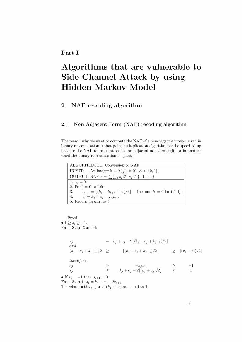
The reason why we want to compute the NAF of a non-negative integer given inbinary representation is that point multiplication algorithm can be speed ed upbecause the NAF representation has no adjacent non-zero digits or in anotherword the binary representation is sparse.
ALGORITHM I.1: Conversion to NAFINPUT: An integer k =
∑l−1j=0 kj2j , kj ∈ {0, 1}.
OUTPUT: NAF k =∑l
j=0 sj2j , sj ∈ {−1, 0, 1}.1. c0 = 0.2. For j = 0 to l do:3. cj+1 = b(kj + kj+1 + cj)/2c (assume ki = 0 for i ≥ l),4. sj = kj + cj − 2cj+1.5. Return (slsl−1...s0).
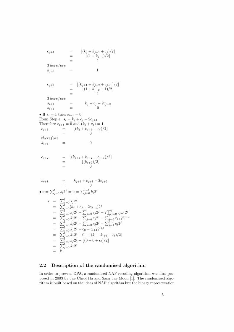
Proof• 1 ≥ si ≥ −1.From Steps 3 and 4:
sj = kj + cj − 2b(kj + cj + kj+1)/2cand(kj + cj + kj+1)/2 ≥ b(kj + cj + kj+1)/2c ≥ b(kj + cj)/2c
thereforesj ≥ −kj+1 ≥ −1sj ≤ kj + cj − 2b(kj + cj)/2c ≤ 1
• If si = −1 then si+1 = 0From Step 4: si = kj + cj − 2cj+1
Therefore both cj+1 and (kj + cj) are equal to 1.
4
cj+1 = b(kj + kj+1 + cj)/2c= b(1 + kj+1)/2c= 1
Thereforekj+1 = 1.
cj+2 = b(kj+1 + kj+2 + cj+1)/2c= b(1 + kj+2 + 1)/2c= 1
Thereforesi+1 = kj + cj − 2cj+2
si+1 = 0
• If si = 1 then si+1 = 0From Step 4: si = kj + cj − 2cj+1
Therefore cj+1 = 0 and (kj + cj) = 1.cj+1 = b(kj + kj+1 + cj)/2c
= 0thereforeki+1 = 0
cj+2 = b(kj+1 + kj+2 + cj+1)/2c= b(kj+2)/2c= 0
si+1 = kj+1 + cj+1 − 2cj+2
= 0
• s =∑l
j=0 si2j = k =∑l−1
j=0 ki2j
s =∑l
j=0 sj2j
=∑l
j=0(kj + cj − 2cj+1)2j
=∑l
j=0 kj2j +∑l
j=0 cj2j − 2∑l
j=0 cj+12j
=∑l
j=0 kj2j +∑l
j=0 cj2j −∑l
j=0 cj+12j+1
=∑l
j=0 kj2j +∑l
j=0 cj2j −∑l+1
j=1 cj2j
=∑l
j=0 kj2j + c0 − cl+12l+1
=∑l
j=0 kj2j + 0− b(kl + kl+1 + cl)/2c=
∑lj=0 kj2j − b(0 + 0 + cl)/2c
=∑l
j=0 kj2j
= k
2.2 Description of the randomised algorithm
In order to prevent DPA, a randomised NAF recoding algorithm was first pro-posed in 2003 by Jae Cheol Ha and Sang Jae Moon [1]. The randomised algo-rithm is built based on the ideas of NAF algorithm but the binary representation
5
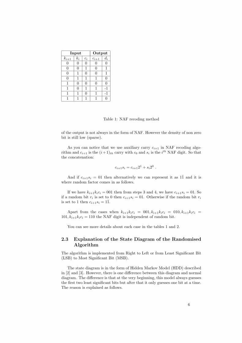
Input Outputki+1 ki ci ci+1 di
0 0 0 0 00 0 1 0 10 1 0 0 10 1 1 1 01 0 0 0 01 0 1 1 -11 1 0 1 -11 1 1 1 0
Table 1: NAF recoding method
of the output is not always in the form of NAF. However the density of non zerobit is still low (sparse).
As you can notice that we use auxiliary carry ci+1 in NAF recoding algo-rithm and ci+1 is the (i+1)th carry with c0 and si is the ith NAF digit. So thatthe concatenation:
ci+1si = ci+121 + si20 .
And if ci+1si = 01 then alternatively we can represent it as 11̄ and it iswhere random factor comes in as follows.
If we have ki+1kici = 001 then from steps 3 and 4, we have ci+1si = 01. Soif a random bit ri is set to 0 then ci+1si = 01. Otherwise if the random bit ri
is set to 1 then ci+1si = 11̄.
Apart from the cases when ki+1kici = 001, ki+1kici = 010, ki+1kici =101, ki+1kici = 110 the NAF digit is independent of random bit.
You can see more details about each case in the tables 1 and 2.
2.3 Explanation of the State Diagram of the RandomisedAlgorithm
The algorithm is implemented from Right to Left or from Least Significant Bit(LSB) to Most Significant Bit (MSB).
The state diagram is in the form of Hidden Markov Model (HDD) describedin [2] and [3]. However, there is one difference between this diagram and normaldiagram. The difference is that at the very beginning, this model always guessesthe first two least significant bits but after that it only guesses one bit at a time.The reason is explained as follows.
6
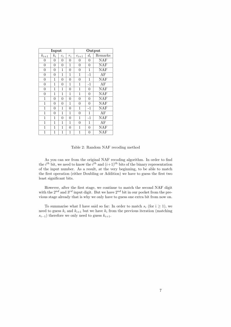
Input Outputki+1 ki ci ri ci+1 di Remarks
0 0 0 0 0 0 NAF0 0 0 1 0 0 NAF0 0 1 0 0 1 NAF0 0 1 1 1 -1 AF0 1 0 0 0 1 NAF0 1 0 1 1 -1 AF0 1 1 0 1 0 NAF0 1 1 1 1 0 NAF1 0 0 0 0 0 NAF1 0 0 1 0 0 NAF1 0 1 0 1 -1 NAF1 0 1 1 0 1 AF1 1 0 0 1 -1 NAF1 1 1 1 0 1 AF1 1 1 0 1 0 NAF1 1 1 1 1 0 NAF
Table 2: Random NAF recoding method
As you can see from the original NAF recoding algorithm. In order to findthe ith bit, we need to know the ith and (i+1)th bits of the binary representationof the input number. As a result, at the very beginning, to be able to matchthe first operation (either Doubling or Addition) we have to guess the first twoleast significant bits.
However, after the first stage, we continue to match the second NAF digitwith the 2nd and 3rd input digit. But we have 2nd bit in our pocket from the pre-vious stage already that is why we only have to guess one extra bit from now on.
To summarise what I have said so far: In order to match si (for i ≥ 1), weneed to guess ki and ki+1 but we have ki from the previous iteration (matchingsi−1) therefore we only need to guess ki+1.
7
Transition Key Bits Probabilityq(n)1 → q
(n+2)10 00 1
q(n)1 → q
(n+2)11 10 1
q(n)1 → q
(n+2)2 01 1
q(n)1 → q
(n+2)3 11 1
q(n)2 → q
(n)13 n/a 1
q(n)3 → q
(n)12 n/a 1
q(n)4 → q
(n)10 n/a 1
q(n)5 → q
(n)11 n/a 1
q(n)6 → q
(n)14 n/a 1
q(n)7 → q
(n)15 n/a 1
q(n)8 → q
(n+1)7 1 1/2
q(n)8 → q
(n+1)5 1 1/2
q(n)8 → q
(n+1)4 0 1/2
q(n)8 → q
(n+1)6 0 1/2
q(n)9 → q
(n+1)9 1 1
q(n)9 → q
(n+1)8 0 1
q(n)10 → q
(n+1)10 0 1
q(n)10 → q
(n+1)11 1 1
q(n)11 → q
(n+1)2 0 1
q(n)11 → q
(n+1)3 1 1
q(n)12 → q
(n+1)2 0 1/2
q(n)12 → q
(n+1)8 0 1/2
q(n)12 → q
(n+1)3 1 1/2
q(n)12 → q
(n+1)9 1 1/2
q(n)13 → q
(n+1)4 0 1/4
q(n)13 → q
(n+1)6 0 1/4
q(n)13 → q
(n+1)10 0 1/2
q(n)13 → q
(n+1)5 1 1/4
q(n)13 → q
(n+1)7 1 1/4
q(n)13 → q
(n+1)11 1 1/2
q(n)14 → q
(n+1)4 0 1/2
q(n)14 → q
(n+1)6 0 1/2
q(n)14 → q
(n+1)5 1 1/2
q(n)14 → q
(n+1)7 1 1/2
q(n)15 → q
(n+1)0 0 1
q(n)15 → q
(n+1)1 1 1
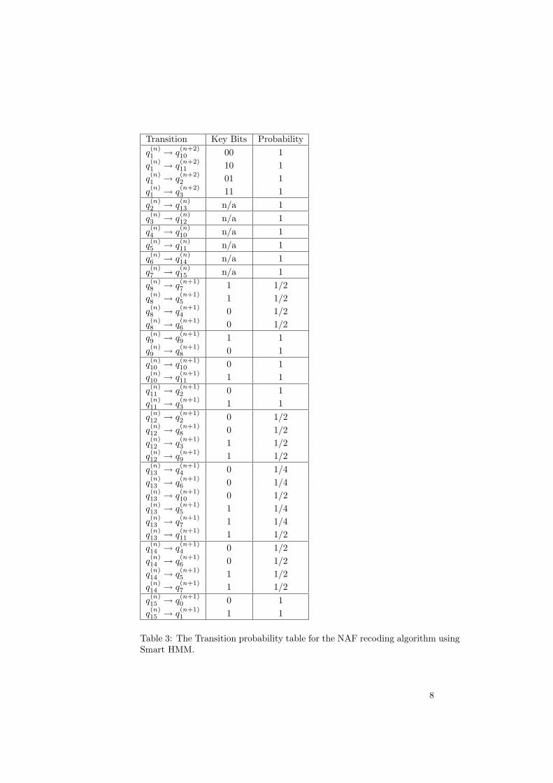
Table 3: The Transition probability table for the NAF recoding algorithm usingSmart HMM.
8
3 Liardet-Smart Algorithm
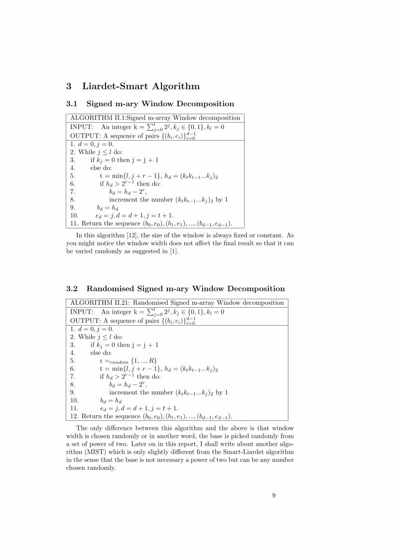
3.1 Signed m-ary Window Decomposition
ALGORITHM II.1:Signed m-array Window decompositionINPUT: An integer k =
∑lj=0 2j , kj ∈ {0, 1}, kl = 0
OUTPUT: A sequence of pairs {(bi, ei)}d−1i=0
1. d = 0, j = 0.2. While j ≤ l do:3. if kj = 0 then j = j + 14. else do:5. t = min{l, j + r − 1}, hd = (ktkt−1...kj)26. if hd > 2r−1 then do:7. bd = hd − 2r,8. increment the number (ktkt−1...kj)2 by 19. bd = hd
10. ed = j, d = d + 1, j = t + 1.11. Return the sequence (b0, e0), (b1, e1), ..., (bd−1, ed−1).
In this algorithm [12], the size of the window is always fixed or constant. Asyou might notice the window width does not affect the final result so that it canbe varied randomly as suggested in [1].
3.2 Randomised Signed m-ary Window Decomposition
ALGORITHM II.21: Randomised Signed m-array Window decompositionINPUT: An integer k =
∑lj=0 2j , kj ∈ {0, 1}, kl = 0
OUTPUT: A sequence of pairs {(bi, ei)}d−1i=0
1. d = 0, j = 0.2. While j ≤ l do:3. if kj = 0 then j = j + 14. else do:5. r =random {1, ..., R}6. t = min{l, j + r − 1}, hd = (ktkt−1...kj)27. if hd > 2r−1 then do:8. bd = hd − 2r,9. increment the number (ktkt−1...kj)2 by 110. bd = hd
11. ed = j, d = d + 1, j = t + 1.12. Return the sequence (b0, e0), (b1, e1), ..., (bd−1, ed−1).
The only difference between this algorithm and the above is that windowwidth is chosen randomly or in another word, the base is picked randomly froma set of power of two. Later on in this report, I shall write about another algo-rithm (MIST) which is only slightly different from the Smart-Liardet algorithmin the sense that the base is not necessary a power of two but can be any numberchosen randomly.
9
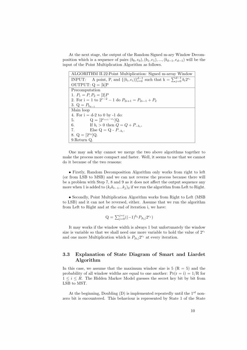
At the next stage, the output of the Random Signed m-ary Window Decom-position which is a sequence of pairs (b0, e0), (b1, e1), ..., (bd−1, ed−1) will be theinput of the Point Multiplication Algorithm as follows.
ALGORITHM II.22:Point Multiplication: Signed m-array WindowINPUT: A point, P, and {(bi, ei)}d−1
i=0 such that k =∑d−1
j=0 bi2ei
OUTPUT: Q = [k]PPrecomputation1. P1 = P, P2 = [2]P2. For i = 1 to 2r−2 − 1 do P2i+1 = P2i−1 + P2
3. Q = Pbd−1
Main loop4. For i = d-2 to 0 by -1 do:5. Q = [2ei+1−ei ]Q.6. If bi > 0 then Q = Q + P−bi
,7. Else Q = Q - P−bi .8. Q = [2e0 ]Q.9.Return Q.
One may ask why cannot we merge the two above algorithms together tomake the process more compact and faster. Well, it seems to me that we cannotdo it because of the two reasons:
• Firstly, Random Decomposition Algorithm only works from right to left(or from LSB to MSB) and we can not reverse the process because there willbe a problem with Step 7, 8 and 9 as it does not affect the output sequence anymore when 1 is added to (ktkt−1...kj)2 if we run the algorithm from Left to Right.
• Secondly, Point Multiplication Algorithm works from Right to Left (MSBto LSB) and it can not be reversed, either. Assume that we run the algorithmfrom Left to Right and at the end of iteration i, we have:
Q =∑j=i
j=0((−1)bj P|bj |2ej )
It may works if the window width is always 1 but unfortunately the windowsize is variable so that we shall need one more variable to hold the value of 2ei
and one more Multiplication which is P|bi|2ei at every iteration.
3.3 Explanation of State Diagram of Smart and LiardetAlgorithm
In this case, we assume that the maximum window size is 5 (R = 5) and theprobability of all window widths are equal to one another: Pr(r = i) = 1/R for1 ≤ i ≤ R. The Hidden Markov Model guesses the secret key bit by bit fromLSB to MST.
At the beginning, Doubling (D) is implemented repeatedly until the 1st non-zero bit is encountered. This behaviour is represented by State 1 of the State
10
Transition Key Bits Probabilityq(n)1 → q
(n+1)1 0 1
q(n)1 → q
(n+1)2 1 1
q(n)2 → q
(n)r+2 n/a 1
q(n)3 → q
(n+1)2 0 1
q(n)3 → q
(n+1)3 1 1
q(n)i → q
(n+1)i+1 for i = 4,...,r 0 or 1 1
q(n)r+1 → q
(n+1)1 0 1
q(n)r+1 → q
(n+1)3 1 1
q(n)r+2 → q
(n+1)1 0 2/r
q(n)r+2 → q
(n+1)2 1 1/r
q(n)r+2 → q
(n+1)3 0 1/r
q(n)r+2 → q
(n+1)i fori = 4, ..., r + 1 0 or 1 1/r
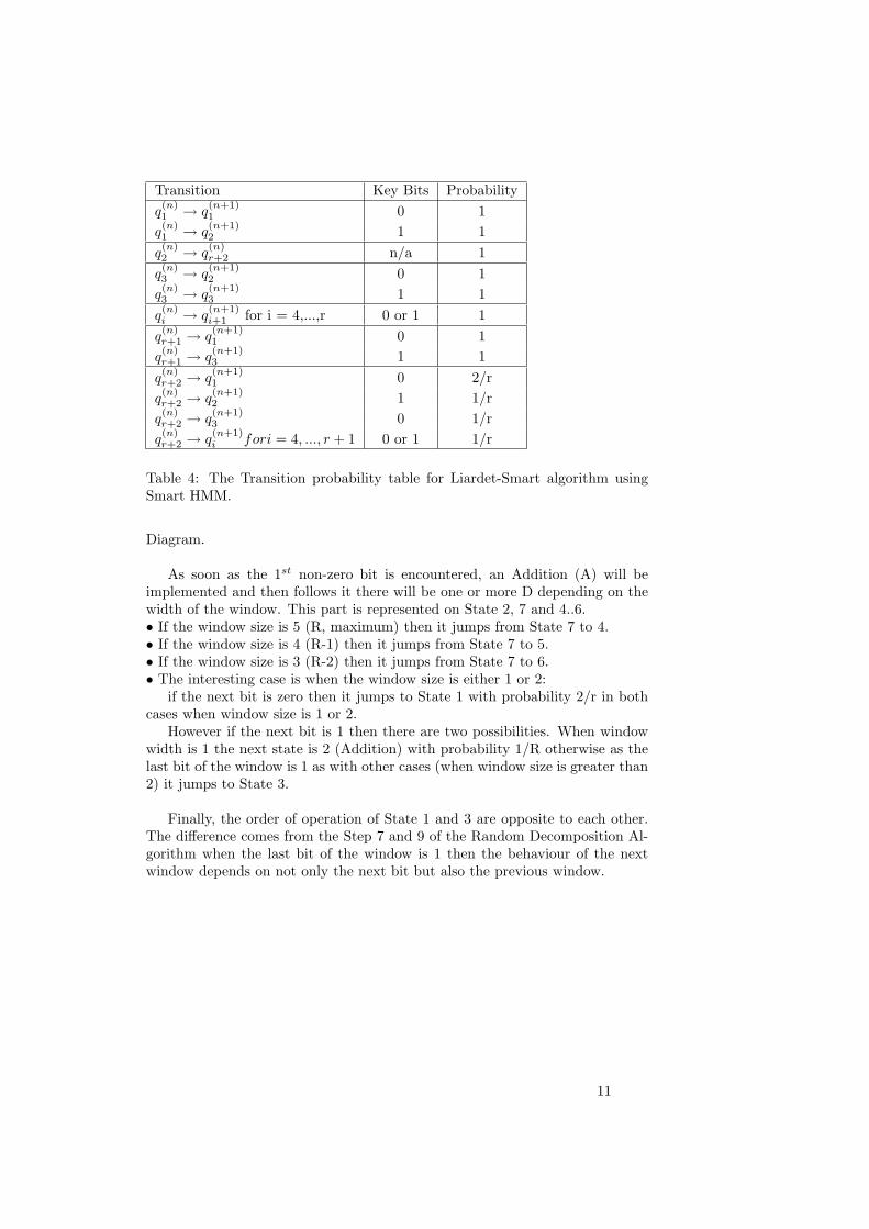
Table 4: The Transition probability table for Liardet-Smart algorithm usingSmart HMM.
Diagram.
As soon as the 1st non-zero bit is encountered, an Addition (A) will beimplemented and then follows it there will be one or more D depending on thewidth of the window. This part is represented on State 2, 7 and 4..6.• If the window size is 5 (R, maximum) then it jumps from State 7 to 4.• If the window size is 4 (R-1) then it jumps from State 7 to 5.• If the window size is 3 (R-2) then it jumps from State 7 to 6.• The interesting case is when the window size is either 1 or 2:
if the next bit is zero then it jumps to State 1 with probability 2/r in bothcases when window size is 1 or 2.
However if the next bit is 1 then there are two possibilities. When windowwidth is 1 the next state is 2 (Addition) with probability 1/R otherwise as thelast bit of the window is 1 as with other cases (when window size is greater than2) it jumps to State 3.
Finally, the order of operation of State 1 and 3 are opposite to each other.The difference comes from the Step 7 and 9 of the Random Decomposition Al-gorithm when the last bit of the window is 1 then the behaviour of the nextwindow depends on not only the next bit but also the previous window.
11
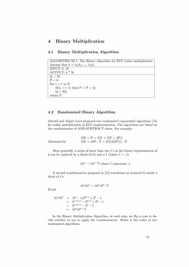
4 Binary Multiplication
4.1 Binary Multiplication Algorithm
ALGORITHM III.1: The Binary Algorithm for ECC scalar multiplicationAssume that k = kNkN−1...k2k1
INPUT: k, MOUTPUT: k * MQ = MP = 0For i = 1 to N
if(ki == 1) then P = P + QQ = 2Q
return P
4.2 Randomised Binary Algorithm
Oswald and Aigner have proposed two randomised exponential algorithms [13]for scalar multiplication in ECC implementation. The algorithms are based onthe randomisation of ADD-SUBTRACT chain. For example:
15P = P + 2(P + 2(P + 2P))Alternatively 15P = 16P - P = 2(2(2(2P))) - P
More generally, a series of more than two 1’s in the binary representation ofk can be replaced by a block of 0’s and a 1̄ (where 1̄ = -1).
01a → 10a−11̄ where 1̄ represents -1
A second transformation proposed in [13] transforms an isolated 0’s inside ablock of 1’s.
01a01b → 10a10b−11̄Proof:
01a01b = (2a − 1)2b+1 + 2b − 1= 2a+b+1 − 2b+1 + 2b − 1= 2a+b+1 − 2b − 1= 10a10b−11̄
In the Binary Multiplication Algorithm, at each step, we flip a coin to de-cide whether or not to apply the transformation. Below is the codes of tworandomised algorithms.
12
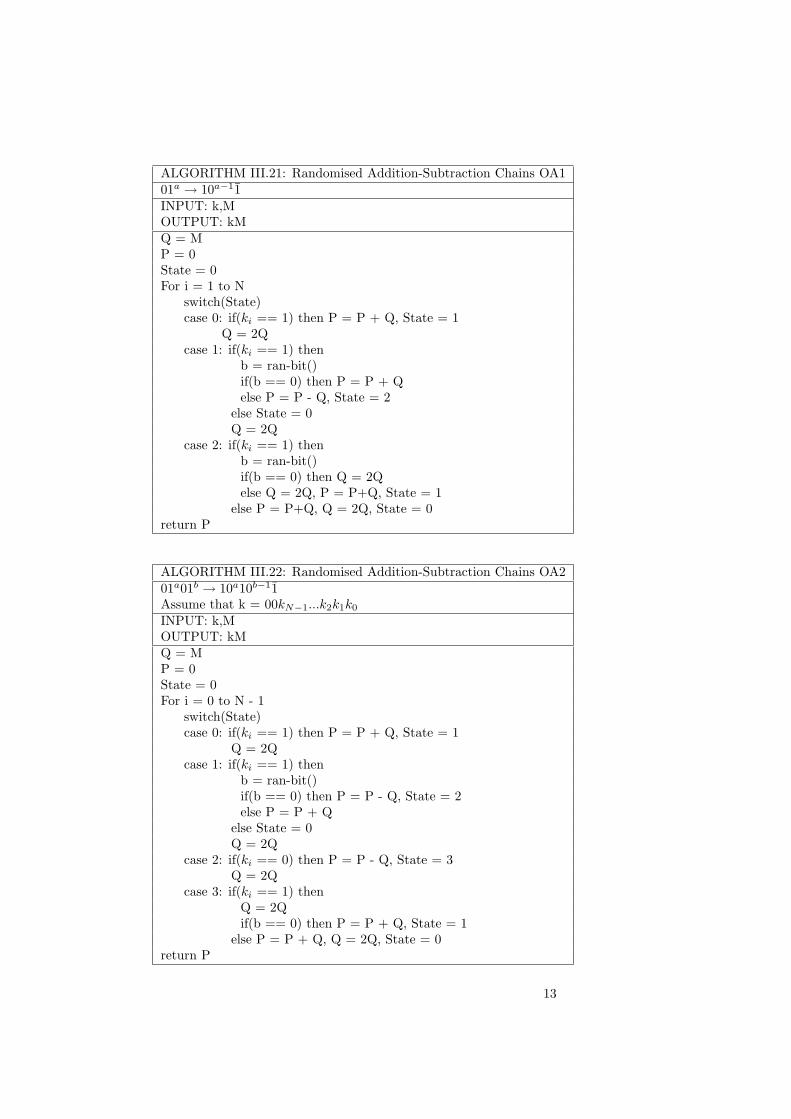
ALGORITHM III.21: Randomised Addition-Subtraction Chains OA101a → 10a−11̄INPUT: k,MOUTPUT: kMQ = MP = 0State = 0For i = 1 to N
switch(State)case 0: if(ki == 1) then P = P + Q, State = 1
Q = 2Qcase 1: if(ki == 1) then
b = ran-bit()if(b == 0) then P = P + Qelse P = P - Q, State = 2
else State = 0Q = 2Q
case 2: if(ki == 1) thenb = ran-bit()if(b == 0) then Q = 2Qelse Q = 2Q, P = P+Q, State = 1
else P = P+Q, Q = 2Q, State = 0return P
ALGORITHM III.22: Randomised Addition-Subtraction Chains OA201a01b → 10a10b−11̄Assume that k = 00kN−1...k2k1k0
INPUT: k,MOUTPUT: kMQ = MP = 0State = 0For i = 0 to N - 1
switch(State)case 0: if(ki == 1) then P = P + Q, State = 1
Q = 2Qcase 1: if(ki == 1) then
b = ran-bit()if(b == 0) then P = P - Q, State = 2else P = P + Q
else State = 0Q = 2Q
case 2: if(ki == 0) then P = P - Q, State = 3Q = 2Q
case 3: if(ki == 1) thenQ = 2Qif(b == 0) then P = P + Q, State = 1
else P = P + Q, Q = 2Q, State = 0return P
13
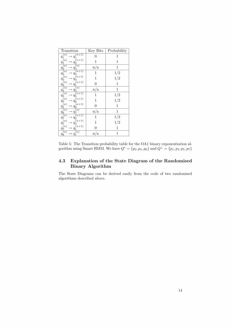
Transition Key Bits Probabilityq(n)1 → q
(n+1)1 0 1
q(n)1 → q
(n+1)2 1 1
q(n)2 → q
(n)3 n/a 1
q(n)3 → q
(n+1)2 1 1/2
q(n)3 → q
(n+1)4 1 1/2
q(n)3 → q
(n+1)1 0 1
q(n)4 → q
(n)5 n/a 1
q(n)5 → q
(n+1)5 1 1/2
q(n)5 → q
(n+1)6 1 1/2
q(n)5 → q
(n+1)8 0 1
q(n)6 → q
(n)7 n/a 1
q(n)7 → q
(n+1)2 1 1/2
q(n)7 → q
(n+1)4 1 1/2
q(n)7 → q
(n+1)1 0 1
q(n)8 → q
(n)1 n/a 1
Table 5: The Transition probability table for the OA1 binary exponentiation al-gorithm using Smart HMM. We have Q∗ = {p2, p4, p6} and Q⊥ = {p1, p3, p5, p7}
4.3 Explanation of the State Diagram of the RandomisedBinary Algorithm
The State Diagrams can be derived easily from the code of two randomisedalgorithms described above.
14
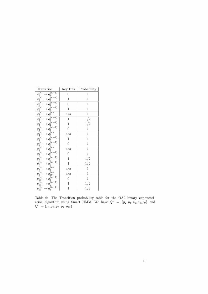
Transition Key Bits Probabilityq(n)0 → q
(n+1)1 0 1
q(n)0 → q
(n+1)2 1 1
q(n)1 → q
(n+1)1 0 1
q(n)1 → q
(n+1)2 1 1
q(n)2 → q
(n)3 n/a 1
q(n)3 → q
(n+1)2 1 1/2
q(n)3 → q
(n+1)4 1 1/2
q(n)3 → q
(n+1)1 0 1
q(n)4 → q
(n)5 n/a 1
q(n)5 → q
(n+1)5 1 1
q(n)5 → q
(n+1)6 0 1
q(n)6 → q
(n)7 n/a 1
q(n)7 → q
(n+1)8 0 1
q(n)7 → q
(n+1)9 1 1/2
q(n)7 → q
(n+1)7 1 1/2
q(n)8 → q
(n)1 n/a 1
q(n)9 → q
(n)10 n/a 1
q(n)10 → q
(n+1)1 0 1
q(n)10 → q
(n+1)2 1 1/2
q(n)10 → q
(n+1)4 1 1/2
Table 6: The Transition probability table for the OA2 binary exponenti-ation algorithm using Smart HMM. We have Q∗ = {p2, p4, p6, p8, p9} andQ⊥ = {p1, p3, p5, p7, p10}
15
Part II
Comparison between two types ofHidden Markov Models (HMM)
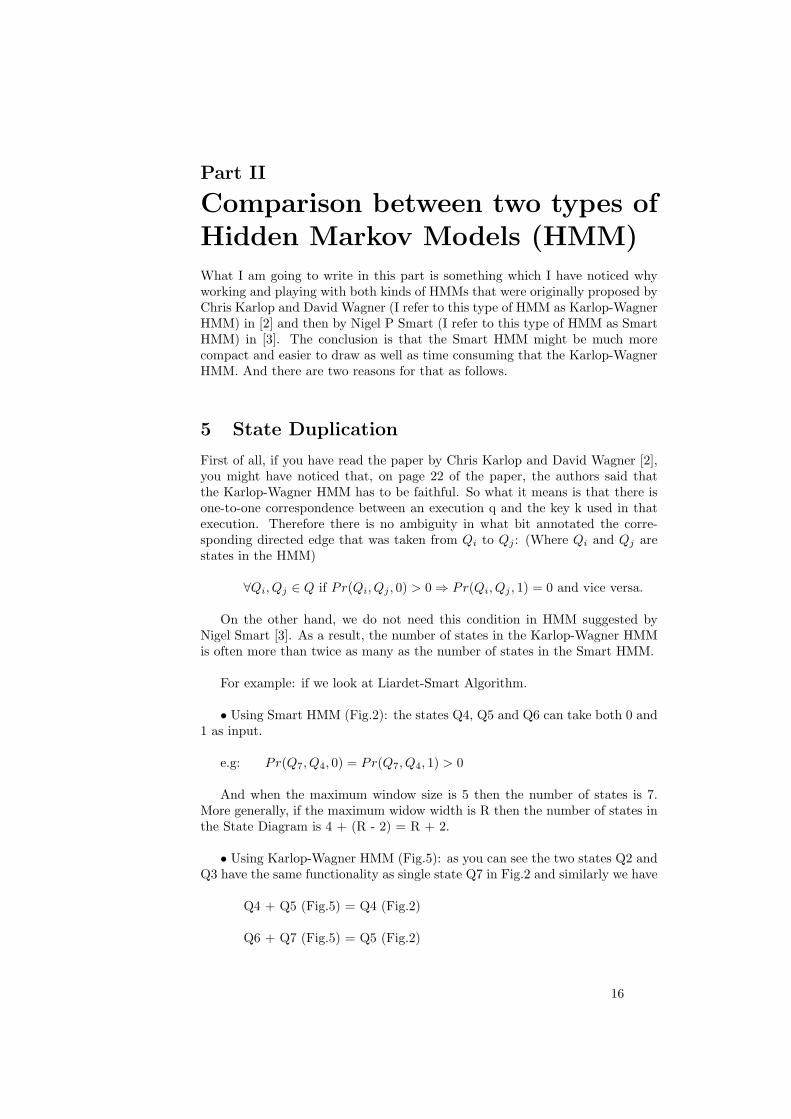
What I am going to write in this part is something which I have noticed whyworking and playing with both kinds of HMMs that were originally proposed byChris Karlop and David Wagner (I refer to this type of HMM as Karlop-WagnerHMM) in [2] and then by Nigel P Smart (I refer to this type of HMM as SmartHMM) in [3]. The conclusion is that the Smart HMM might be much morecompact and easier to draw as well as time consuming that the Karlop-WagnerHMM. And there are two reasons for that as follows.
5 State Duplication
First of all, if you have read the paper by Chris Karlop and David Wagner [2],you might have noticed that, on page 22 of the paper, the authors said thatthe Karlop-Wagner HMM has to be faithful. So what it means is that there isone-to-one correspondence between an execution q and the key k used in thatexecution. Therefore there is no ambiguity in what bit annotated the corre-sponding directed edge that was taken from Qi to Qj : (Where Qi and Qj arestates in the HMM)
∀Qi, Qj ∈ Q if Pr(Qi, Qj , 0) > 0 ⇒ Pr(Qi, Qj , 1) = 0 and vice versa.
On the other hand, we do not need this condition in HMM suggested byNigel Smart [3]. As a result, the number of states in the Karlop-Wagner HMMis often more than twice as many as the number of states in the Smart HMM.
For example: if we look at Liardet-Smart Algorithm.
• Using Smart HMM (Fig.2): the states Q4, Q5 and Q6 can take both 0 and1 as input.
e.g: Pr(Q7, Q4, 0) = Pr(Q7, Q4, 1) > 0
And when the maximum window size is 5 then the number of states is 7.More generally, if the maximum widow width is R then the number of states inthe State Diagram is 4 + (R - 2) = R + 2.
• Using Karlop-Wagner HMM (Fig.5): as you can see the two states Q2 andQ3 have the same functionality as single state Q7 in Fig.2 and similarly we have
Q4 + Q5 (Fig.5) = Q4 (Fig.2)
Q6 + Q7 (Fig.5) = Q5 (Fig.2)
16
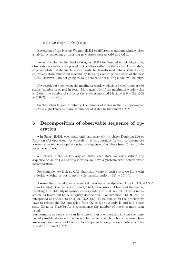
Q8 + Q9 (Fig.5) = Q6 (Fig.2)
Extending of the Karlop-Wagner HMM to different maximum window sizesis trivial by removing or inserting new states such as Q10 and Q11..
We notice that in the Karlop-Wagner HMM for Smart-Liardet Algorithm,observable operations are placed on the edges rather on the states. Fortunately,edge annotated state machine can easily be transformed into a semanticallyequivalent state annotated machine by treating each edge as a state of the newHMM. However I am not going to do it here as the resulting model will be huge.
If we work out then when the maximum window width is 5 then there are 30states (number of edges) in total. More generally, if the maximum window sizeis R then the number of states in the State Annotated Machine is 6 + 2[2(R-2)+ 2(R-2)] = 8R - 10.
So that when R goes to infinity, the number of states in the Karlop-WagnerHMM is eight times as many as number of states in the Smart HMM.
6 Decomposition of observable sequence of op-eration
• In Smart HMM, each state only can carry with it either Doubling (D) orAddition (A) operation. As a result, it is very straight forward to decomposea observable sequence operation into a sequence of symbols from O (set of ob-servable symbols).
• However in the Karlop-Wagner HMM, each state can carry with it anysequence of As or Ds and this is where we have a problem with deterministicdecomposition.
For example: we look at OA1 algorithm where at each state, we flip a cointo decide whether or not to apply this transformation : 01a = 10a−11̄
Assume that it would be convenient if our observable alphabet O = {D,AD,AAD}∗.From Fig.6(a) , the transition from Q2 to Q1 executes a D first and then an A,resulting in a DA output symbol corresponding to that key bit. This is unde-sirable as traces fail to be uniquely decode-able. For instance: DADD can beinterpreted as either (DA,D,D) or (D,AD,D). To be able to fix the problem wehave to relabel the DA transition from Q2 to Q1 to simply D and add a newstate Q3 as in Fig.6(b) As a consequence the number of states is more thanusual.Furthermore, as each state can have more than one operation so that the num-ber of possible states with same number of As and Ds is big a because thereare many combination of Ds and As compared to only two symbols which areA and D in Smart HMM.
17
Transition Key Bits Probabilityq(n)1 → q
(n+1)1 0 1
q(n)1 → q
(n+1)4 1 1
q(n)2 → q
(n+1)1 0 1
q(n)2 → q
(n+1)4 1 1
q(n)3 → q
(n+1)2 0 1
q(n)3 → q
(n+1)3 1 1/2
q(n)3 → q
(n+1)11 1 1/2
q(n)4 → q
(n+1)5 0 1
q(n)4 → q
(n+1)6 1 1/2
q(n)4 → q
(n+1)9 1 1/2
q(n)5 → q
(n+1)1 0 1
q(n)5 → q
(n+1)4 1 1
q(n)6 → q
(n+1)2 0 1
q(n)6 → q
(n+1)3 1 1/2
q(n)6 → q
(n+1)11 1 1/2
q(n)7 → q
(n+1)1 0 1
q(n)7 → q
(n+1)4 1 1
q(n)8 → q
(n+1)5 0 1
q(n)8 → q
(n+1)6 1 1/2
q(n)8 → q
(n+1)9 1 1/2
q(n)9 → q
(n+1)5 0 1
q(n)9 → q
(n+1)6 1 1/2
q(n)9 → q
(n+1)9 1 1/2
q(n)10 → q
(n+1)2 0 1
q(n)10 → q
(n+1)3 1 1/2
q(n)10 → q
(n+1)11 1 1/2
q(n)11 → q
(n+1)7 0 1
q(n)11 → q
(n+1)8 1 1/2
q(n)11 → q
(n+1)10 1 1/2
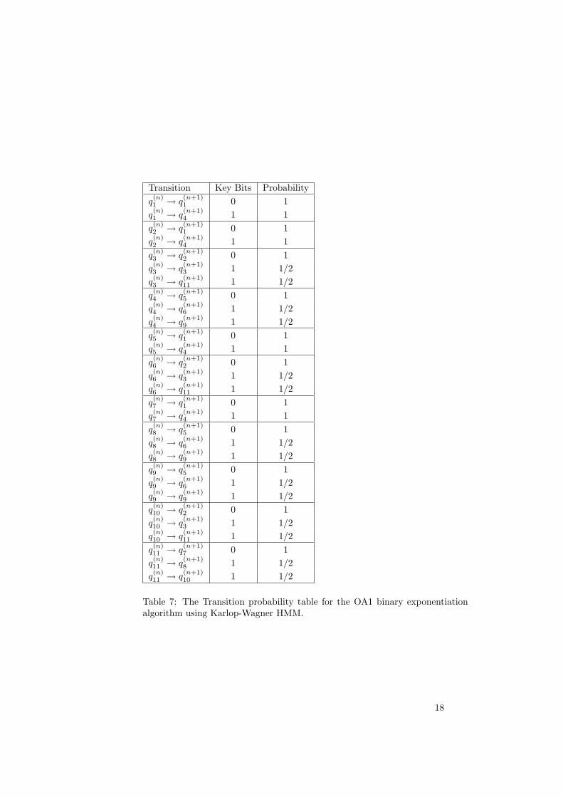
Table 7: The Transition probability table for the OA1 binary exponentiationalgorithm using Karlop-Wagner HMM.
18
Transition Key Bits Probabilityq(n)1 → q
(n+1)1 0 1
q(n)1 → q
(n+1)3 1 1
q(n)2 → q
(n+1)11 0 1
q(n)2 → q
(n+1)2 1 1
q(n)3 → q
(n+1)4 0 1
q(n)3 → q
(n+1)9 1 1/2
q(n)3 → q
(n+1)5 1 1/2
q(n)4 → q
(n+1)1 0 1
q(n)4 → q
(n+1)3 1 1
q(n)5 → q
(n+1)11 0 1
q(n)5 → q
(n+1)2 1 1
q(n)6 → q
(n+1)1 0 1
q(n)6 → q
(n+1)3 1 1
q(n)7 → q
(n+1)1 0 1
q(n)7 → q
(n+1)3 1 1
q(n)8 → q
(n+1)4 0 1
q(n)8 → q
(n+1)9 1 1/2
q(n)8 → q
(n+1)5 1 1/2
q(n)9 → q
(n+1)4 0 1
q(n)9 → q
(n+1)9 1 1/2
q(n)9 → q
(n+1)5 1 1/2
q(n)10 → q
(n+1)11 0 1
q(n)10 → q
(n+1)2 1 1
q(n)11 → q
(n+1)6 0 1
q(n)11 → q
(n+1)12 1 1/2
q(n)11 → q
(n+1)13 1 1/2
q(n)12 → q
(n+1)7 0 1
q(n)12 → q
(n+1)8 1 1/2
q(n)12 → q
(n+1)10 1 1/2
q(n)13 → q
(n+1)6 0 1
q(n)13 → q
(n+1)12 1 1/2
q(n)13 → q
(n+1)13 1 1/2
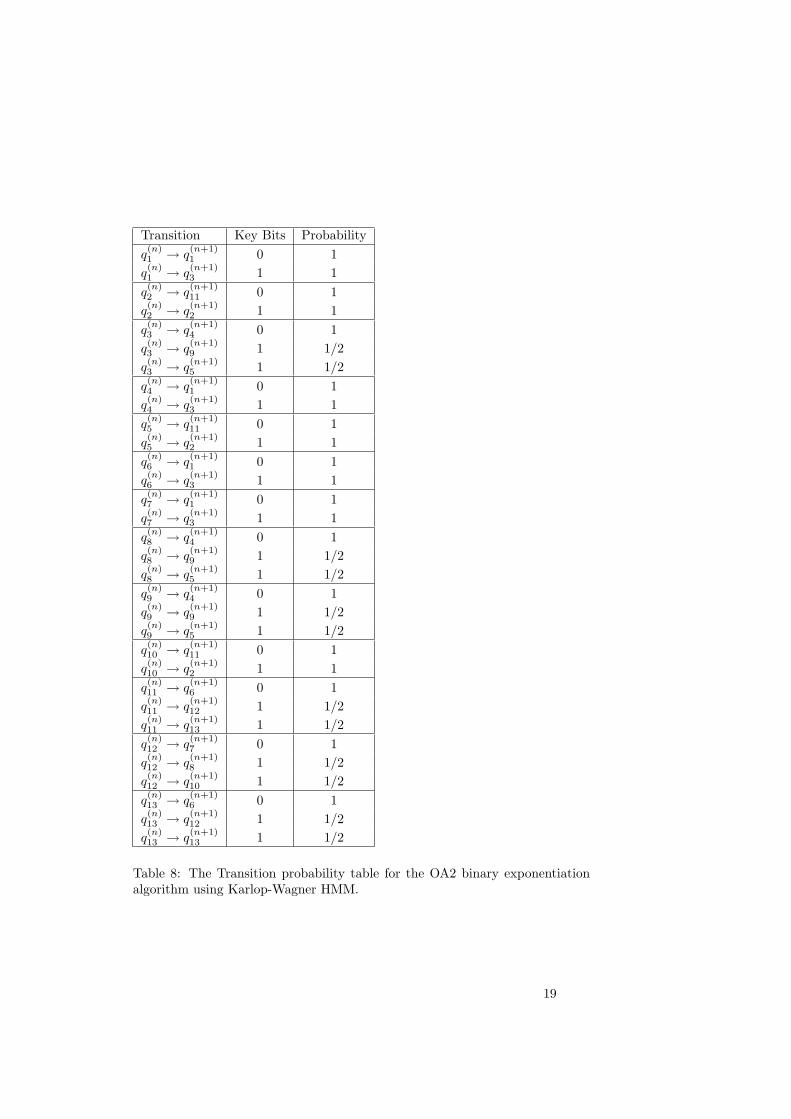
Table 8: The Transition probability table for the OA2 binary exponentiationalgorithm using Karlop-Wagner HMM.
19
Part III
Randomised Algorithms that aresecure against HMM
In this part , I shall discuss a number of randomised algorithms that can not beattacked by Input Hidden Markov Model with explanation why not. In somecases we still can draw HMM for them but it does not mean they are vulnerableto side channel attack.
All algorithms discussed in this part are different ways of randomised de-composition.
7 Overlapping Window method and SimplifyingMIST-Liardet-Smart algorithms
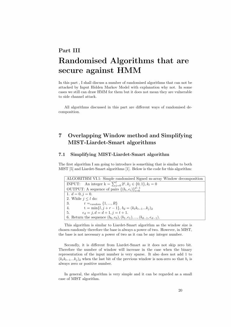
7.1 Simplifying MIST-Liardet-Smart algorithm
The first algorithm I am going to introduce is something that is similar to bothMIST [5] and Liardet-Smart algorithms [1]. Below is the code for this algorithm:
ALGORITHM VI.1: Simple randomised Signed m-array Window decompositionINPUT: An integer k =
∑lj=0 2j , kj ∈ {0, 1}, kl = 0
OUTPUT: A sequence of pairs {(bi, ei)}d−1i=0
1. d = 0, j = 0.2. While j ≤ l do:3. r =random {1, ..., R}4. t = min{l, j + r − 1}, bd = (ktkt−1...kj)25. ed = j, d = d + 1, j = t + 1.6. Return the sequence (b0, e0), (b1, e1), ..., (bd−1, ed−1).
This algorithm is similar to Liardet-Smart algorithm as the window size ischosen randomly therefore the base is always a power of two. However, in MIST,the base is not necessary a power of two as it can be any integer number.
Secondly, it is different from Liardet-Smart as it does not skip zero bit.Therefore the number of window will increase in the case when the binaryrepresentation of the input number is very sparse. It also does not add 1 to(ktkt−1...kj)2 when the last bit of the previous window is non-zero so that bi isalways zero or positive number.
In general, the algorithm is very simple and it can be regarded as a smallcase of MIST algorithm.
20
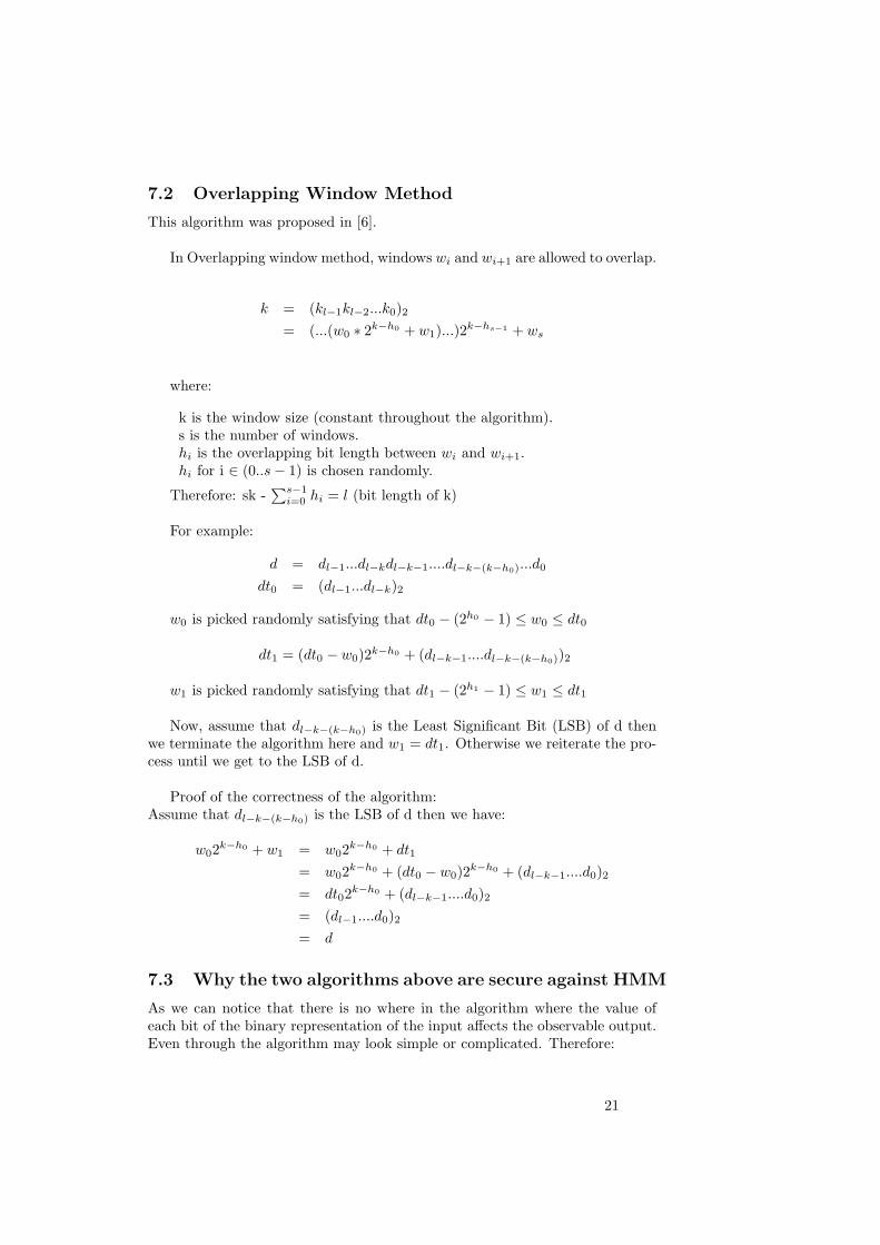
7.2 Overlapping Window Method
This algorithm was proposed in [6].
In Overlapping window method, windows wi and wi+1 are allowed to overlap.
k = (kl−1kl−2...k0)2= (...(w0 ∗ 2k−h0 + w1)...)2k−hs−1 + ws
where:
k is the window size (constant throughout the algorithm).s is the number of windows.hi is the overlapping bit length between wi and wi+1.hi for i ∈ (0..s− 1) is chosen randomly.
Therefore: sk -∑s−1
i=0 hi = l (bit length of k)
For example:
d = dl−1...dl−kdl−k−1....dl−k−(k−h0)...d0
dt0 = (dl−1...dl−k)2
w0 is picked randomly satisfying that dt0 − (2h0 − 1) ≤ w0 ≤ dt0
dt1 = (dt0 − w0)2k−h0 + (dl−k−1....dl−k−(k−h0))2
w1 is picked randomly satisfying that dt1 − (2h1 − 1) ≤ w1 ≤ dt1
Now, assume that dl−k−(k−h0) is the Least Significant Bit (LSB) of d thenwe terminate the algorithm here and w1 = dt1. Otherwise we reiterate the pro-cess until we get to the LSB of d.
Proof of the correctness of the algorithm:Assume that dl−k−(k−h0) is the LSB of d then we have:
w02k−h0 + w1 = w02k−h0 + dt1
= w02k−h0 + (dt0 − w0)2k−h0 + (dl−k−1....d0)2= dt02k−h0 + (dl−k−1....d0)2= (dl−1....d0)2= d
7.3 Why the two algorithms above are secure against HMM
As we can notice that there is no where in the algorithm where the value ofeach bit of the binary representation of the input affects the observable output.Even through the algorithm may look simple or complicated. Therefore:
21
Pr(output = D | ki = 0) = Pr(output = D | ki = 1) = 1/2and Pr(output = A | ki = 0) = Pr(output = A | ki = 1) = 1/2
So that we have achieved maximum entropy and that means the algorithmsare not vulnerable to DPA attack.
8 Flexible Countermeasure using Fractional Win-dow Method
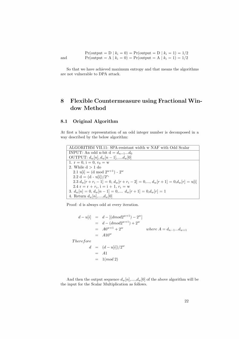
8.1 Original Algorithm
At first a binary representation of an odd integer number is decomposed in away described by the below algorithm:
ALGORITHM VII.11: SPA-resistant width w NAF with Odd ScalarINPUT: An odd n-bit d = dn−1...d0
OUTPUT: dw[n], dw[n− 1], ....dw[0]1. r = 0, i = 0, r0 = w2. While d > 1 do
2.1 u[i] = (d mod 2w+1) - 2w
2.2 d = (d - u[i])/2ri
2.3 dw[r + ri − 1] = 0, dw[r + ri − 2] = 0,..., dw[r + 1] = 0,dw[r] = u[i]2.4 r = r + ri, i = i + 1, ri = w
3. dw[n] = 0, dw[n− 1] = 0,.... dw[r + 1] = 0,dw[r] = 14. Return dw[n],....,dw[0]
Proof: d is always odd at every iteration.
d− u[i] = d− [(dmod2w+1)− 2w]= d− (dmod2w+1) + 2w
= A0w+1 + 2w where A = dn−1...dw+1
= A10w
Therefore
d = (d− u[i])/2w
= A1= 1(mod 2)
And then the output sequence dw[n],....,dw[0] of the above algorithm will bethe input for the Scalar Multiplication as follows.
22
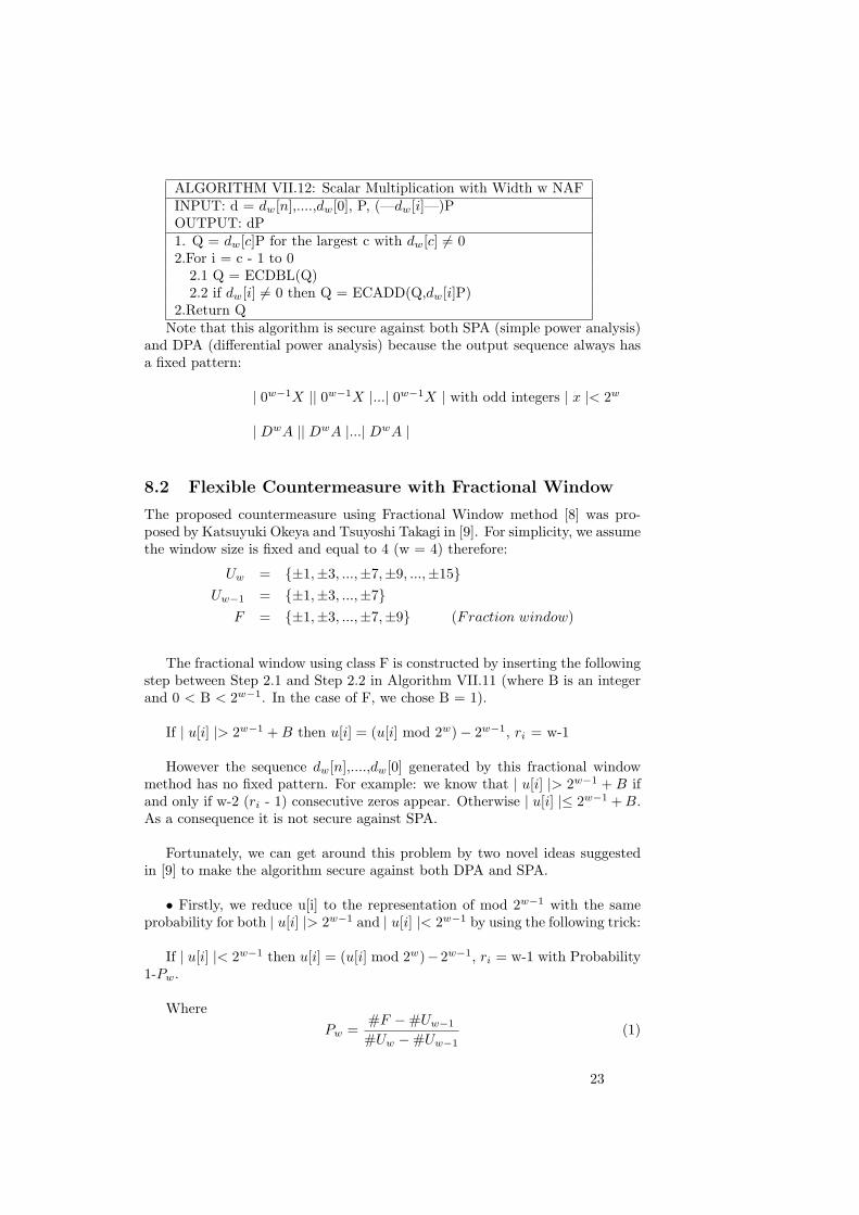
ALGORITHM VII.12: Scalar Multiplication with Width w NAFINPUT: d = dw[n],....,dw[0], P, (—dw[i]—)POUTPUT: dP1. Q = dw[c]P for the largest c with dw[c] 6= 02.For i = c - 1 to 0
2.1 Q = ECDBL(Q)2.2 if dw[i] 6= 0 then Q = ECADD(Q,dw[i]P)
2.Return QNote that this algorithm is secure against both SPA (simple power analysis)
and DPA (differential power analysis) because the output sequence always hasa fixed pattern:
| 0w−1X || 0w−1X |...| 0w−1X | with odd integers | x |< 2w
| DwA || DwA |...| DwA |
8.2 Flexible Countermeasure with Fractional Window
The proposed countermeasure using Fractional Window method [8] was pro-posed by Katsuyuki Okeya and Tsuyoshi Takagi in [9]. For simplicity, we assumethe window size is fixed and equal to 4 (w = 4) therefore:
Uw = {±1,±3, ...,±7,±9, ...,±15}Uw−1 = {±1,±3, ...,±7}
F = {±1,±3, ...,±7,±9} (Fraction window)
The fractional window using class F is constructed by inserting the followingstep between Step 2.1 and Step 2.2 in Algorithm VII.11 (where B is an integerand 0 < B < 2w−1. In the case of F, we chose B = 1).
If | u[i] |> 2w−1 + B then u[i] = (u[i] mod 2w)− 2w−1, ri = w-1
However the sequence dw[n],....,dw[0] generated by this fractional windowmethod has no fixed pattern. For example: we know that | u[i] |> 2w−1 + B ifand only if w-2 (ri - 1) consecutive zeros appear. Otherwise | u[i] |≤ 2w−1 + B.As a consequence it is not secure against SPA.
Fortunately, we can get around this problem by two novel ideas suggestedin [9] to make the algorithm secure against both DPA and SPA.
• Firstly, we reduce u[i] to the representation of mod 2w−1 with the sameprobability for both | u[i] |> 2w−1 and | u[i] |< 2w−1 by using the following trick:
If | u[i] |< 2w−1 then u[i] = (u[i] mod 2w)−2w−1, ri = w-1 with Probability1-Pw.
WherePw =
#F −#Uw−1
#Uw −#Uw−1(1)
23
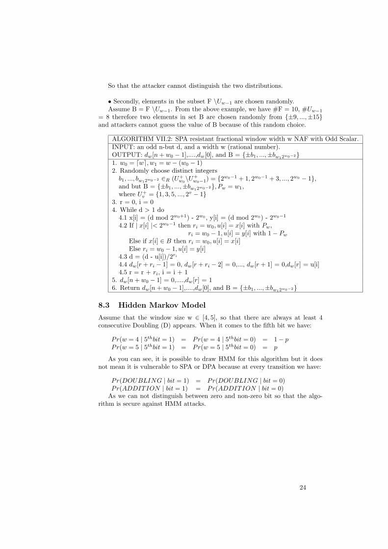
So that the attacker cannot distinguish the two distributions.
• Secondly, elements in the subset F \Uw−1 are chosen randomly.Assume B = F \Uw−1. From the above example, we have #F = 10, #Uw−1
= 8 therefore two elements in set B are chosen randomly from {±9, ...,±15}and attackers cannot guess the value of B because of this random choice.
ALGORITHM VII.2: SPA resistant fractional window width w NAF with Odd Scalar.INPUT: an odd n-but d, and a width w (rational number).OUTPUT: dw[n + w0 − 1],....,dw[0], and B = {±b1, ...,±bw12w0−2}1. w0 = dwe, w1 = w − (w0 − 1)2. Randomly choose distinct integers
b1, ..., bw12w0−2 ∈R (U+w0\U+
w0−1) = {2w0−1 + 1, 2w0−1 + 3, ..., 2w0 − 1},and but B = {±b1, ...,±bw12w0−2}, Pw = w1,where U+
v = {1, 3, 5, ..., 2v − 1}3. r = 0, i = 04. While d > 1 do
4.1 x[i] = (d mod 2w0+1) - 2w0 , y[i] = (d mod 2w0) - 2w0−1
4.2 If | x[i] |< 2w0−1 then ri = w0, u[i] = x[i] with Pw,ri = w0 − 1, u[i] = y[i] with 1− Pw
Else if x[i] ∈ B then ri = w0, u[i] = x[i]Else ri = w0 − 1, u[i] = y[i]
4.3 d = (d - u[i])/2ri
4.4 dw[r + ri − 1] = 0, dw[r + ri − 2] = 0,..., dw[r + 1] = 0,dw[r] = u[i]4.5 r = r + ri, i = i + 1
5. dw[n + w0 − 1] = 0,....,dw[r] = 16. Return dw[n + w0 − 1],....,dw[0], and B = {±b1, ...,±bw12w0−2}
8.3 Hidden Markov Model
Assume that the window size w ∈ [4, 5], so that there are always at least 4consecutive Doubling (D) appears. When it comes to the fifth bit we have:
Pr(w = 4 | 5thbit = 1) = Pr(w = 4 | 5thbit = 0) = 1− pPr(w = 5 | 5thbit = 1) = Pr(w = 5 | 5thbit = 0) = p
As you can see, it is possible to draw HMM for this algorithm but it doesnot mean it is vulnerable to SPA or DPA because at every transition we have:
Pr(DOUBLING | bit = 1) = Pr(DOUBLING | bit = 0)Pr(ADDITION | bit = 1) = Pr(ADDITION | bit = 0)
As we can not distinguish between zero and non-zero bit so that the algo-rithm is secure against HMM attacks.
24
9 Conclusion and Future Work
In this project, I have looked at six randomised exponentiation algorithms, threeof them are vulnerable to side channel attacks via IDHMM and another threeare not. I also have done some comparisons between two types of IDHMMsproposed in [2] and [3] used to model side channel attacks.
Further work still needs to be carried out. For example: I have not imple-mented a tool that takes a Smart HMM of an algorithm and a set of output tracesas inputs and returns the correspondent secret key. Therefore, it is not clear atthe moment, whether or not Smart HMM is actually faster than Karlop-WagnerHMM, even through I can prove that for the same randomised algorithm, SmartHMM tends to be more compact and easier to draw than Karlop-Wagner HMM.
In addition, apart from the six algorithms discussed in this report, I alsolooked at other randomised algorithms such as Random register renaming tofoil DPA proposed by David May in [10], Add and Double always method in [11]and Mongomery Ladder in [11]. However, it is quite trivial that these algorithmsare secure against HMM as they always produce fixed pattern output traces.
The conclusion I can draw from here is that Input-Driven Hidden MarkovModel can only attack algorithms that work or make decision and choice basedon the value of particular bits of the binary representation of a secret key.
25
References
[1] Liardet,P.Y.., Smart, N..: Preventing SPA/DPA in ECC Systems Using theJacobi Form. In: Third International Workshop on Cryptographic Hard-ware and Embedded Systems (CHES).(2001)
[2] Chris Karlop and Davis Wagner: Hidden Markov Model Cryptanalysis
[3] Nigel P Smart: Further Hidden Markov Model Cryptanalysis
[4] Jae Cheol Ha and Snag Jae Moon: Randomised Signed-Scalar Multiplica-tion of ECC to Resist Power Attacks. In: Fourth International Workshopon Cryptographic Hardware and Embedded Systems (CHES).(2002)
[5] Colin D.Walter: Mist: An Efficient, Randomized Exponentiation Algo-rithm for Resisting Power Analysis. In: RSA 2002-Cryptographers’ Track.(2002)
[6] Kouichi Itoh, Jun Yajima, Masahiko Takenaka and Naoya Torii: DPACountermeasure by Improving the Window Method. In: Fourth Inter-national Workshop on Cryptographic Hardware and Embedded Systems(CHES).(2002)
[7] Colin D.Walter: Breaking the Liardet-Smart Randomized ExponentiationAlgorithm. In: Fifth Smart Card Research and Advanced Application Con-ference (CARDIS). (2002)
[8] Bodo Moller: Improved Techniques for Fast Exponentiation. In: thefifth International Conference on Information Security and Cryptography(ICISC 2002) LNCS 2578, (2003), 298-312
[9] A More Flexible Countermeasure against Side Channel Attacks Using Win-dow Method
[10] D. May, H.L. Muller and N.P Smart: Random Register Renaming to FoilDPA. In: Third International Workshop on Cryptographic Hardware andEmbedded Systems (CHES).(2001)
[11] Kouichi Itoh, Tetsuya Izu and Masahiko Takenaka: A Practical Counter-measure against Address-Bit Differential Power Analysis
[12] I.F.Blake, G.Seroussi and N.P.Smart. Elliptic Curve in cryptography. Cam-bridge University Press, 1999.
[13] Elisabeth Oswald and Manfred Aigner: Randomized Addition-SubtractionChains as a Countermeasure against Power Attacks. In: Third Inter-national Workshop on Cryptographic Hardware and Embedded Systems(CHES).(2001)
26